DEDICATION

ToFadil & Soad; My Parents

Randa; My wifeFadil & Nour; My Lovely

Kids

All there love and influence will remain with me always

i

Thanks Family

ii

ACKNOWLEDGEMENT

I am very grateful to my supervisor Prof. Dr. Doğan İbrahim for providing his overall

wisdom, counsel, direction, encouragement and assistance throughout the duration of

my thesis.

I would like to express my gratitude and thanks to Prof. Dr. Fakhreddin Mamedov,

Assoc.Prof.Dr Rahib Abiyev, Assoc.Prof.Dr Adnan Khashman, and Assoc. Prof. Dr.

Feridun Muradov for their support and valuable advice given throughout the duration

of my studies for the Degree of Master of Science at the Near East University.

And a big thank to my family that supports me in every step I take in this life and one of

these steps is achieving Masters Degree at this university (NEU), and I would like to

make use of this chance to thank my mother, father, brothers and my sisters.

I would like to express my deepest gratitude for the constant support, understanding

and love that I received from my wife Randa during the past years.

Finally, I will not forget the people who supported me in North Cyprus and made me

enjoy the last two years I spent studying; especially Özatay Family, Hakkı Şahlan and

Mehmet Cancuri.

iii

ABSTRACT

Data compression is an important field of information technology because of the

reduced data communication and storage costs it achieves. The continued increase in the

amount of data that needs to be transferred or archived nowadays, is the reason for

increasing the importance of data compression. Data compression is implemented using

several data compression methods. One of these methods is Huffman algorithm, which

has been successfully applied in the field of data compression.

The goal of this thesis is software development of lossless algorithm for compressing

Latin characters based languages text files by reducing the amount of redundancy in the

coding of symbols. The design of a compression system with concentrating on Turkish

language requires careful attention to the following issues: Frequencies of letters in the

text file, the Turkish alphabet consists of 29 letters, three letters of the Turkish alphabet

are not included in the ASCII code, and Turkish alphabet has some special characters

which are not included in other languages.

In this thesis a computer program for the compression of Turkish text was developed.

The program has been applied to totally unconstrained computerized Turkish text files.

iv

TABLE OF CONTENTS

DEDICATION................................................................................................................i

ACKNOWLEDGEMENT..............................................................................................ii

ABSTRACT....................................................................................................................iii

TABLE OF CONTENTS...............................................................................................iv

LIST OF FIGURES.....................................................................................................viii

LIST OF TABLES..........................................................................................................ix

INTRODUCTION...........................................................................................................1

DATA COMPRESSION TERMINOLOGY.................................................................3

CHAPTER 1 : DATA COMPRESSION BACKGROUND.........................................4

1.1 Overview.................................................................................................................4

1.2 Importance of Data Compression............................................................................4

1.3 History of Data Compression Development............................................................4

1.4 Physical and Logical Compression.........................................................................5

1.5 Symmetric and Asymmetric Compression..............................................................6

1.6 Adaptive, Semi-Adaptive, and Non-Adaptive Encoding........................................7

1.7 Loosy and Lossless Compression............................................................................7

1.8 Compression algorithms input/output strategy........................................................8

1.9 Classifications of Compression algorithms strategy...............................................9

1.10 Data Types to be compressed................................................................................9

1.10.1 Speech compression...................................................................................9

1.10.2 Image and video compression..................................................................10

1.10.3 Text compression......................................................................................10

1.11 Summary:............................................................................................................10

CHAPTER 2 : TURKISH LANGUAGE SPECIFICATIONS..................................11

2.1 Overview...............................................................................................................11

2.2 Introduction...........................................................................................................11

2.3 A Short History of the Turkish Language.............................................................12

2.4 The New Script......................................................................................................13

2.5 The Turkish Alphabet............................................................................................14

2.6 The Turkish Vocabulary........................................................................................14

2.7 Turkish Grammar..................................................................................................15

v

2.8 Encoding Standards...............................................................................................15

2.9 Turkish Keyboard Standards.................................................................................16

2.10 Typographic Issues..............................................................................................17

2.11 Mixing Scripts.....................................................................................................17

2.12 Linguistic Characteristics of English and Turkish..............................................17

2.13 Statistical Data Based On Static Language Elements.........................................18

2.14 Corpus Statistics..................................................................................................20

2.15 Other statistics.....................................................................................................23

2.16 Summary:............................................................................................................23

CHAPTER 3 : TEXT COMPRESSION ALGORITHMS.........................................24

3.1 Overview...............................................................................................................24

3.2 Introduction...........................................................................................................24

3.3 Compression paradigm..........................................................................................25

3.4 Compression algorithm categories........................................................................25

3.4.1 Statistical Compressor................................................................................26

3.4.1.1 Symbol frequency................................................................................26

3.4.1.2 Huffman Algorithm.............................................................................26

3.4.1.2.1 History...........................................................................................27

3.4.1.2.2 Huffman Encoding........................................................................27

3.4.1.2.3 Prefix-Free Property......................................................................28

3.4.1.2.4 Binary Trees..................................................................................30

3.4.1.2.5 Algorithm for creating a Huffman binary tree..............................31

3.4.1.2.6 Construction of a binary tree for Huffman Coding.......................31

3.4.1.2.7 Obtaining Huffman code from the Tree........................................35

3.4.1.2.8 Advantages and Disadvantages.....................................................36

3.4.2 Dictionary Model Compressor...................................................................37

3.4.2.1 Lempel Ziv Compression Algorithm...................................................37

3.4.2.1.1 History...........................................................................................37

3.4.2.1.2 LZW CODING..............................................................................38

3.4.2.1.3 Description of LZW Algorithm.....................................................38

3.4.2.1.4 How Does LZW Compression Algorithm Work...........................38

3.4.2.1.5 Decompression..............................................................................42

3.4.2.1.6 How Does LZW Decompression Algorithm Work.......................42

vi

3.4.2.1.7 Facts about LZW Algorithm.........................................................43

3.4.3 Transformation Based Compression Technique.........................................44

3.4.3.1 History.................................................................................................44

3.4.3.2 Pre-Compression Transformations......................................................45

3.4.3.3 Transformation Based Compress Paradigm........................................45

3.4.3.4 Star-Encoding......................................................................................46

3.4.3.4.1 An Example of Star Encoding.......................................................46

3.5 Summary................................................................................................................47

CHAPTER 4 : DEVELOPMENT OF TEXT COMPRESSION PROGRAM.........48

4.1 Overview...............................................................................................................48

4.2 The Developed application program.....................................................................48

4.3 Turkish alphabets coding:......................................................................................48

4.4 The Application algorithm....................................................................................49

4.5 Two Examples:......................................................................................................50

4.6 The User application Interface..............................................................................52

4.7 Software Development language...........................................................................52

4.7.1 Why Visual Basic 6.0?...............................................................................52

4.8 Parts of the program listing...................................................................................53

4.9 . Functions of the application program interfaces.................................................55

4.9.1 Radio Buttons.............................................................................................55

4.9.2 Command buttons.......................................................................................56

4.9.3 Text boxes..................................................................................................56

4.9.4 Text list.......................................................................................................57

4.9.5 Graph tool...................................................................................................58

4.10 Summary..............................................................................................................58

CHAPTER 5 : RESULTS OF SIMULATION...........................................................59

5.1 Overview...............................................................................................................59

5.2 Files to be compressed...........................................................................................59

5.3 Compressing a file.................................................................................................59

5.3.1 Original text file.........................................................................................59

5.3.2 File after compression................................................................................60

5.4 Applying compression using the program.............................................................60

5.5 Summary................................................................................................................62

vii

CONCLUSION..............................................................................................................63

REFERENCES..............................................................................................................64

APPENDIX A: LISTING OF SOURCE CODE.......................................................A-1

APPENDIX B: ENGLISH LANGUAGE ALPHABETS.........................................B-1

APPENDIX C: TURKISH LANGUAGE ALPHABETS........................................C-1

viii

LIST OF FIGURES

Figure 2.1 Turkish Q Keyboard style.............................................................................16

Figure 2.2 Turkish F Keyboard style..............................................................................16

Figure 3.1 Text compression and decompression..........................................................25

Figure 3.2 Ordering characters from highest to lowest frequency.................................32

Figure 3.3 Combined frequencies of the lowest 2 nodes................................................32

Figure 3.4 Combinations of lowest frequency nodes.....................................................33

Figure 3.5 Combinations of lowest frequency nodes.....................................................33

Figure 3.6 Combinations between tow nodes.................................................................34

Figure 3.7 Combinations between tow nodes.................................................................34

Figure 3.8 Last combination of nodes which result binary Huffman tree......................35

Figure 3.9 Assigning 0s for the right side of the tress and 1s for the left side...............35

Figure 3.10 Text compression paradigm with lossless, reversible transformation........45

Figure 4.1 Flowchart of the application algorithm.........................................................50

Figure 4.2 creating a binary tree, (a) without moving, (b) with moving characters.......51

Figure 4.3 creating a binary tree, (a) without moving, (b) with moving characters.......51

Figure 4.4 User interface of the application developed by the author............................52

Figure 4.5 Activating the compress part of the program................................................55

Figure 4.6 Activating the de-compress part of the program...........................................56

Figure 4.7 Text boxes used on the program...................................................................57

Figure 4.8 The text list used to display the letter frequency of the project....................57

Figure 4.9 Letter frequencies shown in graphical shape................................................58

Figure 5.1 An example of file after compression...........................................................60

ix

LIST OF TABLES

Table1.1 Algorithms, (a) lossy/lossless, (b) input/output strategy, classifications...........9

Table 2.1 The Turkish Alphabet.....................................................................................14

Table 2.2 Linguistic characteristics of English and Turkish..........................................17

Table 3.1 ASCII code and Generated code for some characters....................................29

Table 3.2 A generated prefix free code for English alphabet.........................................30

Table 3.3 Letter frequencies in a text file to be compressed..........................................32

Table 3.4 Original ASCII codes and generated codes for letters in the above example 36

Table 3.5 Generated dictionary for the above text..........................................................41

Table 3.6 Regenerating dictionary from a compressed file............................................42

Table 5.1 Original file sizes tested using the program...................................................59

Table 5.2 Result of applying the compression program on Doc files.............................61

Table 5.3 Result of applying the compression program on txt files...............................61

x

INTRODUCTION

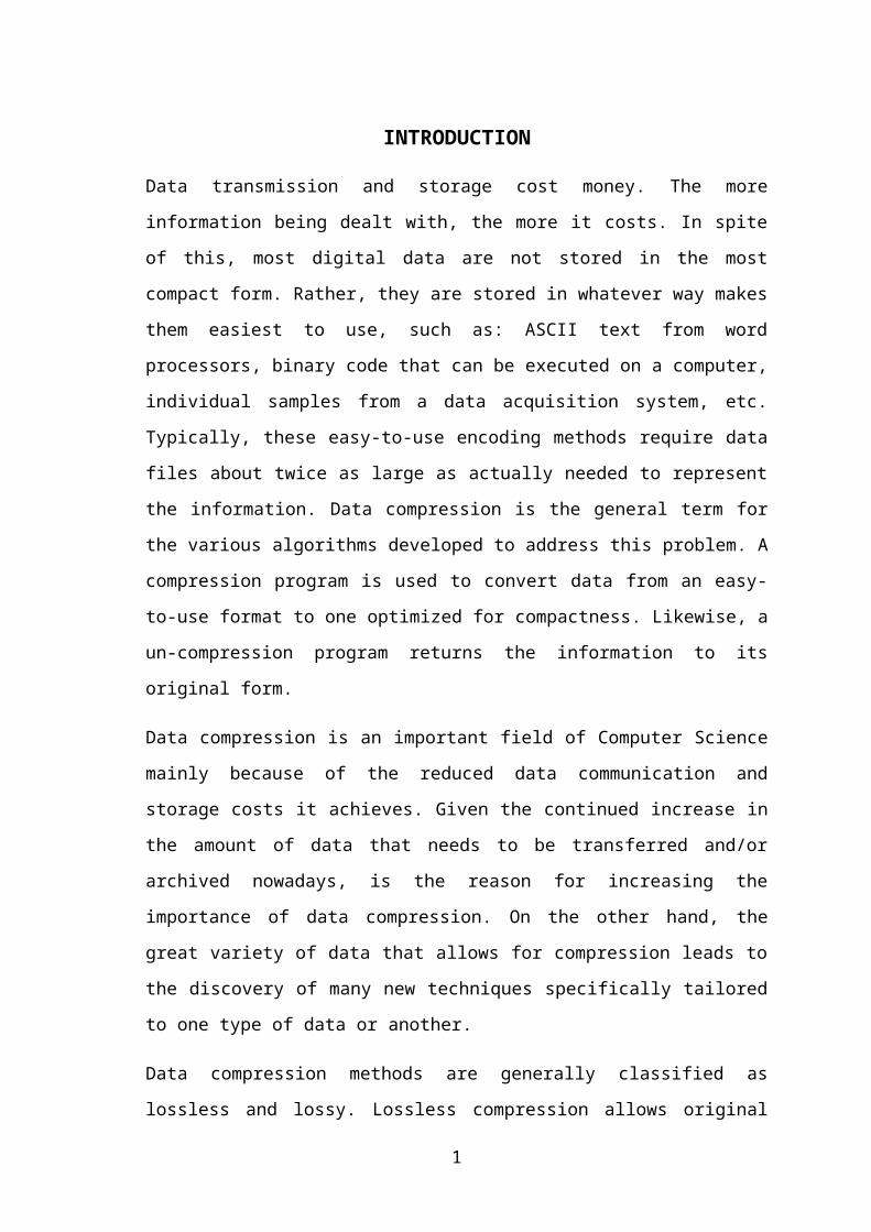
Data transmission and storage cost money. The more information being dealt with, the

more it costs. In spite of this, most digital data are not stored in the most compact form.

Rather, they are stored in whatever way makes them easiest to use, such as: ASCII text

from word processors, binary code that can be executed on a computer, individual

samples from a data acquisition system, etc. Typically, these easy-to-use encoding

methods require data files about twice as large as actually needed to represent the

information. Data compression is the general term for the various algorithms developed

to address this problem. A compression program is used to convert data from an easy-

to-use format to one optimized for compactness. Likewise, a un-compression program

returns the information to its original form.

Data compression is an important field of Computer Science mainly because of the

reduced data communication and storage costs it achieves. Given the continued increase

in the amount of data that needs to be transferred and/or archived nowadays, is the

reason for increasing the importance of data compression. On the other hand, the great

variety of data that allows for compression leads to the discovery of many new

techniques specifically tailored to one type of data or another.

Data compression methods are generally classified as lossless and lossy. Lossless

compression allows original data to be recovered exactly. Although used for text data,

lossless compression is useful in special classes of images, such as medical imaging,

finger print data and astronomical images and databases containing mostly vital

numerical data, tables and text information. In contrast, lossy compression schemes

allow some deterioration and are generally used for video, audio and still image

applications. The deterioration of the quality of lossy images are usually not detectable

by human perceptual system, and the compression system exploit this by a process

called ‘Quantization’ to achieve compression by a factor of 10 to a couple of hundreds.

Thesis Objective

The objectives of this thesis research are to develop software for compressing Turkish

language text files. This thesis presents a text compression system using Huffman

algorithm although it has a decompression system. The main feature of the thesis for

compression is reducing the amount of redundancy in the coding of symbols. To

1

achieve this target, instead of using the ASCII code which is fixed 8 bits for each

character for storing data, we will generate a smaller code for each character. The

generated new code may be fixed length but smaller than 8 bits, or a variable-length

coding system that assigns smaller codes for more frequently used characters and larger

codes for less frequently used characters in order to reduce the size of files being

compressed.

Thesis Outline

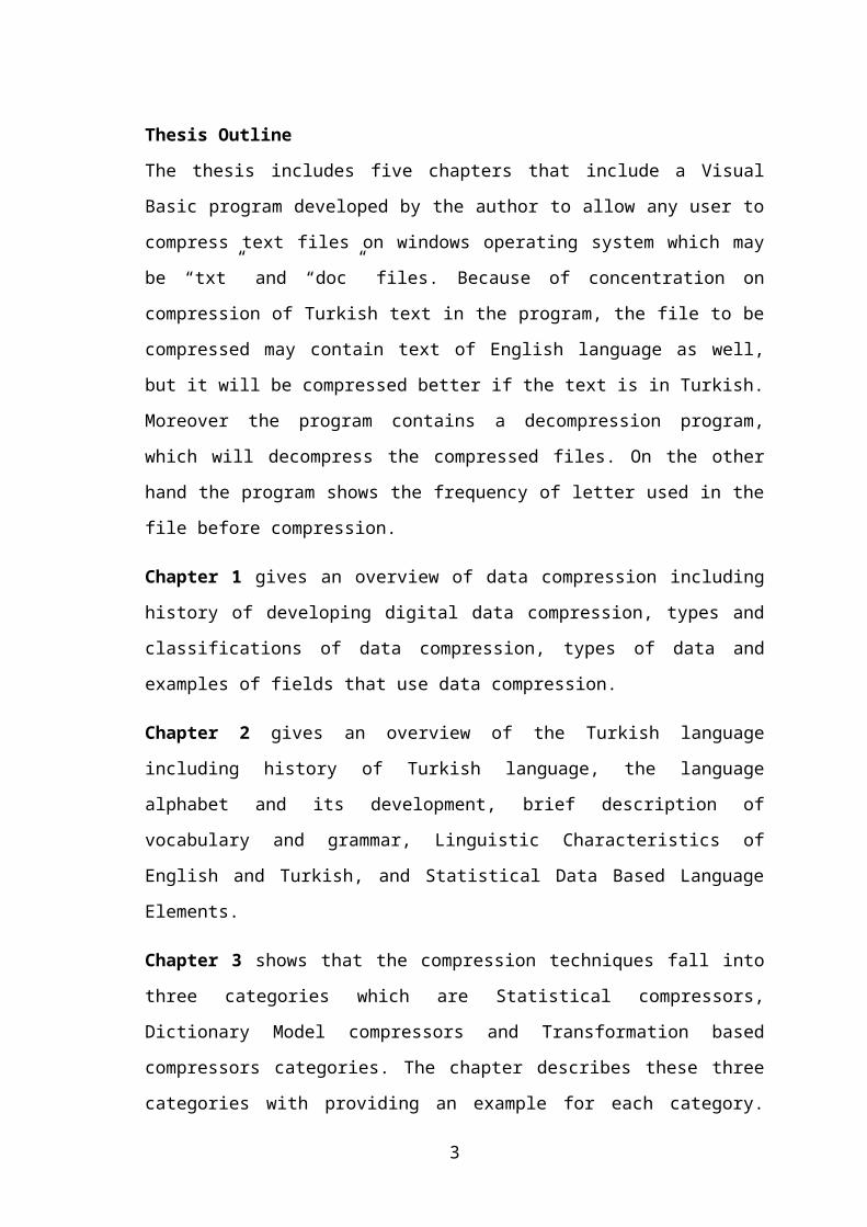
The thesis includes five chapters that include a Visual Basic program developed by the

author to allow any user to compress text files on windows operating system which may

be “txt” and “doc” files. Because of concentration on compression of Turkish text in the

program, the file to be compressed may contain text of English language as well, but it

will be compressed better if the text is in Turkish. Moreover the program contains a

decompression program, which will decompress the compressed files. On the other

hand the program shows the frequency of letter used in the file before compression.

Chapter 1 gives an overview of data compression including history of developing

digital data compression, types and classifications of data compression, types of data

and examples of fields that use data compression.

Chapter 2 gives an overview of the Turkish language including history of Turkish

language, the language alphabet and its development, brief description of vocabulary

and grammar, Linguistic Characteristics of English and Turkish, and Statistical Data

Based Language Elements.

Chapter 3 shows that the compression techniques fall into three categories which are

Statistical compressors, Dictionary Model compressors and Transformation based

compressors categories. The chapter describes these three categories with providing an

example for each category. This thesis concentrates on statistical compression category

especially on Huffman algorithm.

Chapter 4 describes the application program developed by the author and shows its

interfaces and describes the function of each component of it.

Chapter 5 shows the results of applying the program developed to compress some files.

The program is applied on 14 files of deferent sizes.

2

DATA COMPRESSION TERMINOLOGY

Below is a list of some commonly used terms which may be encountered while reading

this thesis:

Compression: decreasing the size of any computerized file size in a new file, the result

file is an unreadable file unless it is de-compressed.

Encoding: It is a way of compressing computerized files by giving new code for the

characters (letters).

Original File: The text file before it has been compressed

Encoded Data And Compressed Data: describe the same information after it has been

compressed.

Un-Encoded Data And Raw Data: describe data before it has been compressed, and

the terms.

Compression Algorithm: is the method that used to compress or to encode a

computerized data file.

Huffman Coding Algorithm: is the algorithm I used to develop the application

program for my thesis.

Compression Ratio: is used to refer to the ratio of uncompressed data to compressed

data. Thus, a 10:1 compression ratio is considered five times more efficient than 2:1. Of

course, data compressed using an algorithm yielding 10:1 compression is five times

smaller than the same data compressed using an algorithm yielding 2:1 compression. In

practice, because only image data is normally compressed, analysis of compression

ratios provided by various algorithms must take into account the absolute sizes of the

files tested.

3

CHAPTER 1 : DATA COMPRESSION BACKGROUND

1.1 Overview

In this chapter we will give an overview of Data compression for better understanding

of what will be described in next chapters.

This chapter will show the importance and a brief history of developing data

compression. Moreover it will describe the classifications of data compression. In

addition, it will talk about types of data that could be compressed giving examples about

fields that make use of data compression.

1.2 Importance of Data Compression

Images transmitted over the World Wide Web are an excellent example of why data

compression is important, and the effectiveness of lossless versus lossy compression.

Suppose we need to download a detailed color image over a computer's 33.6 kbps

modem. If the image is not compressed (a TIFF file, for example), it will contain about

600 Kbytes of data. If it has been compressed using a lossless technique (such as used in

the GIF format), it will be about one-half this size, or 300 Kbytes. If lossy compression

has been used (a JPEG file), it will be about 50 Kbytes. The point is, the download

times for these three equivalent files are 142 seconds, 71 seconds, and 12 seconds,

respectively. [11] That's a big difference! It's no wonder you seldom see TIFF images on

the web. JPEG is usually used for acquired images, such as photographs; while GIF is used

for line art, such as logos.

1.3 History of Data Compression Development

Morse code, invented in 1838 for use in telegraphy, is an early example of data

compression based on using shorter codewords for letters such as "e" and "t" that are

more common in English. [31]

The late 40's were the early years of Information Theory; the idea of developing

efficient new coding methods was just starting to be fleshed out. Ideas of entropy,

information content and redundancy were explored. One popular notion held that if the

probability of symbols in a message were known, there ought to be a way to code the

symbols so that the message will take up less space. [27] In 1949 Claude Shannon and

4

Robert Fano devised a systematic way to assign codewords based on probabilities of

blocks. An optimal method for doing this was then found by David Huffman in 1951.

Early implementations were typically done in hardware, with specific choices of

codewords being made as compromises between compression and error correction. In

the mid-1970s, the idea emerged of dynamically updating codewords for Huffman

encoding, based on the actual data encountered. And in the late 1970s, with online

storage of text files becoming common, software compression programs began to be

developed, almost all based on adaptive Huffman coding.[31]

In 1977 Abraham Lempel and Jacob Ziv suggested the basic idea of pointer-based

encoding. In the mid-1980s, following work by Terry Welch, the so-called LZW

algorithm rapidly became the method of choice for most general-purpose compression

systems. It was used in programs such as PKZIP, as well as in hardware devices such as

modems. In the late 1980s, digital images became more common, and standards for

compressing them emerged. In the early 1990s, lossy compression methods also began

to be widely used.

1.4 Physical and Logical Compression

Compression algorithms are often described as squeezing, squashing, crunching, or

imploding data, but these are not very accurate descriptions of what is actually

happening. Although the major use of compression is to make data use less disk space,

compression does not actually physically cram the data into a smaller size package in

any meaningful sense. [6]

Instead, compression algorithms are used to re-encode data into a different, more

compact representation conveying the same information. In other words, fewer words

are used to convey the same meaning, without actually saying the same thing.

The distinction between physical and logical compression methods is made on the basis

of how the data is compressed or, more precisely, how the data is rearranged into a

more compact form. Physical compression is performed on data exclusive of the

information it contains; it only translates a series of bits from one pattern to another,

more compact one. While the resulting compressed data may be related to the original

data in a mechanical way, that relationship will not be obvious to us.

5

Physical compression methods typically produce strings of gibberish, at least relative to

the information content of the original data. The resulting block of compressed data is

normally smaller than the original because the physical compression algorithm has

removed the redundancy that existed in the data itself. [6]

Logical compression is accomplished through the process of logical substitution that is,

replacing one alphabetic, numeric, or binary symbol with another. Changing "United

States of America" to "USA" is a good example of logical substitution, because "USA"

is derived directly from the information contained in the string "United States of

America" and retains some of its meaning. In a similar fashion "can't" can be logically

substituted for "cannot". Logical compression works only on data at the character level

or higher and is based exclusively on information contained within the data. Logical

compression is generally not used in image data compression. [6]

1.5 Symmetric and Asymmetric Compression

Compression algorithms can also be divided into two categories: symmetric and

asymmetric. A symmetric compression method uses roughly the same algorithms, and

performs the same amount of work, for compression as it does for decompression. For

example, a data transmission application where compression and decompression are

both being done on the fly will usually require a symmetric algorithm for the greatest

efficiency.

Asymmetric methods require substantially more work to go in one direction than they

require in the other. Usually, the compression step takes far more time and system

resources than the decompression step. In the real world this makes sense. For example,

if we are making an image database in which an image will be compressed once for

storage, but decompressed many times for viewing, then we can probably tolerate a

much longer time for compression than for decompression. An asymmetric algorithm

that uses much CPU time for compression, but is quick to decode, would work well in

this case.

Algorithms that are asymmetric in the other direction are less common but have some

applications. In making routine backup files, for example, we fully expect that many of

the backup files will never be read. A fast compression algorithm that is expensive to

decompress might be useful in this case. [6]

6

1.6 Adaptive, Semi-Adaptive, and Non-Adaptive Encoding

Non-adaptive encoders are certain dictionary-based encoders, which are designed to

compress only specific types of data. These non-adaptive encoders contain a static

dictionary of predefined substrings that are known to occur with high frequency in the

data to be encoded. A non-adaptive encoder designed specifically to compress English

language text would contain a dictionary with predefined substrings such as "and",

"but", and "the", because these substrings appear very frequently in English text. [6]

An adaptive encoder, on the other hand, carries no preconceived heuristics about the

data it is to compress. Adaptive compressors, achieve data independence by building

their dictionaries completely from scratch. They do not have a predefined list of static

substrings and instead build phrases dynamically as they encode.

Adaptive compression is capable of adjusting to any type of data input and of returning

output using the best possible compression ratio. This is in contrast to non-adaptive

compressors, which are capable of efficiently encoding only a very select type of input

data for which they are designed.

A mixture of these two dictionary encoding methods is the semi-adaptive encoding

method. A semi-adaptive encoder makes an initial pass over the data to build the

dictionary and a second pass to perform the actual encoding. Using this method, an

optimal dictionary is constructed before any encoding is actually performed.

1.7 Loosy and Lossless Compression

The majority of compression scheme we deal within this thesis is called lossless. A

lossless technique means that the restored (decompressed) data file is identical to the

original (compressed) one. When a chunk of data is compressed and then

decompressed, the original information contained in the data is preserved. No data has

been lost or discarded; the data has not been changed in any way. This is absolutely

necessary for many types of data, for example: executable code, text files, word

processing files, tabulated numbers, etc. You cannot afford to misplace even a single bit

of this type of information.

In comparison, data files that represent images and other acquired signals do not have to

be kept in perfect condition for storage or transmission. All real world measurements

7

inherently contain a certain amount of noise. If the changes made to these signals

resemble a small amount of additional noise, no harm is done. Compression techniques

that allow this type of degradation are called lossy. This distinction is important because

lossy techniques are much more effective at compression than lossless methods. The

higher the compression ratio, the more noise added to the data. [19]

Lossy compression methods, however, throw away some of the data in an image in

order to achieve compression ratios better than that of most lossless compression

methods. Some methods contain elaborate heuristic algorithms that adjust themselves to

give the maximum amount of compression while changing as little of the visible detail

of the image as possible. Other less elegant algorithms might simply discard a least

significant portion of each pixel, and, in terms of image quality, hope for the best.

The terms lossy and lossless are sometimes erroneously used to describe the quality of a

compressed image. Some people assume that if any image data is lost, this could only

degrade the image. The assumption is that we would never want to lose any data at all.

This is certainly true if our data consists of text or numerical data that is associated with

a file, such as a spreadsheet or a chapter of a novel.

1.8 Compression algorithms input/output strategy

Most data compression programs operate by taking a group of data from the original

file, compressing it in some way, and then writing the compressed group to the output

file. For instance, one of the audio compression techniques is CS&Q, short for Coarser

Sampling and/or Quantization. Suppose we are compressing a digitized waveform, such

as an audio signal that has been digitized to 12 bits. We might read two adjacent

samples from the original file (24 bits), discard one of the samples completely, discard

the least significant 4 bits from the other sample, and then write the remaining 8 bits to

the output file. With 24 bits in and 8 bits out, we have implemented a 3:1 compression

ratio using a lossy algorithm. While this is rather crude in itself, it is very effective

when used with a technique called transform compression. [11]

CS&Q is called a fixed-input fixed-output scheme. That is, a fixed number of bits are

read from the input file and a smaller fixed number of bits are written to the output file.

Other compression methods allow a variable number of bits to be read or written.

8

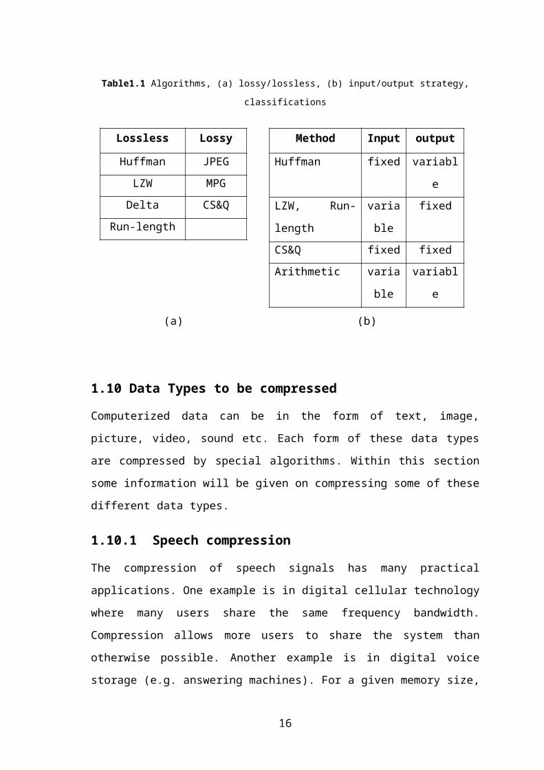
1.9 Classifications of Compression algorithms strategy

As mentioned before data compression algorithms can be categorized in many different

ways. In the tables below we will show two classification types of compression

algorithms. Lossless/lossy is an important classification type for compression

algorithms, will be shown in (Table 1.1(a)) for some compression techniques. [11]

Another type of classification is input/output strategy which is shown in (Table 1.1(b)).

In this table JPEG and MPEG image compression techniques are not listed, because

they are composite algorithms that combine many of the other techniques and are too

sophisticated to be classified into these simple categories.

Table1.1 Algorithms, (a) lossy/lossless, (b) input/output strategy, classifications

Lossless Lossy

Huffman JPEG

LZW MPG

Delta CS&Q

Run-length

Method Input output

Huffman fixed variable

LZW, Run-length variable fixed

CS&Q fixed fixed

Arithmetic variable variable

(a) (b)

1.10 Data Types to be compressed

Computerized data can be in the form of text, image, picture, video, sound etc. Each

form of these data types are compressed by special algorithms. Within this section some

information will be given on compressing some of these different data types.

1.10.1 Speech compression

The compression of speech signals has many practical applications. One example is in

digital cellular technology where many users share the same frequency bandwidth.

Compression allows more users to share the system than otherwise possible. Another

example is in digital voice storage (e.g. answering machines). For a given memory size,

compression allows longer messages to be stored than otherwise. [25]

9

Historically, digital speech signals are sampled at a rate of 8000 samples/sec. Typically,

each sample is represented by 8 bits (using mu-law). This corresponds to an

uncompressed rate of 64 kbps (kbits/sec). With current compression techniques (all of

which are lossy), it is possible to reduce the rate to 8 kbps with almost no perceptible

loss in quality. Further compression is possible at a cost of lower quality. [25]

1.10.2 Image and video compression

Computer imaging is a fascinating and exciting area to be involved in today. Computer

imaging can be defined as the acquisition and processing of visual information by

computer. One of the manipulated processes on images is compression. Image

compression is recognized as an enabling technology and it is the natural technology for

handling the increased spatial resolutions of today’s imaging sensors. Image

compression plays a major role in many important and diverse applications, including

televideo conferencing, remote sensing.

In practice, a small change in the value of a pixel may well be invisible, especially in

high-resolution images where a single pixel is barely visible anyway. [25]

1.10.3 Text compression

Text compression is one of the widest applications of compression algorithms. In this

thesis we are investigating only text compression, mainly the compression of text based

on Turkish characters.

1.11 Summary:

This chapter has explained the importance and a brief history of developing data

compression. Moreover it described the classifications of data compression. In addition,

it talked about types of computer data that could be compressed.

10

CHAPTER 2 : TURKISH LANGUAGE SPECIFICATIONS

2.1 Overview

In this chapter, we present statistical information about the structure and the usage of

Turkish Language. Statistical data analysis is divided into two groups: static data

analysis and dynamic data analysis. The former one takes into account all the parts of

the structure of the language, while the latter one concerns with the daily usage.

The benefits obtained from statistical analysis are that, we can get important

information about the language as a whole and it will be helpful to develop

computerized language applications.

2.2 Introduction

Turkish is a member of the south-western or Oghuz group of the Turkic languages,

which also includes Turkmen, Azerbaijani or Azeri, Ghasghai and Gagauz. The Turkish

language uses a Latin alphabet consisting of twenty-nine letters, of which eight are

vowels and twenty-one are consonants. Unlike the main Indo-European languages (such

as French and German), Turkish is an example of an agglutinative language, where

words are a combination of several morphemes and suffixes. Here, words contain a root

and suffixes are combined with this root in order to extend its meaning or to create other

classes of words. In Turkish the process of adding one suffix to another can result in

relatively long words, which often contain an amount of semantic information

equivalent to a whole English phrase, clause or sentence. Due to this complex

morphological structure, a single Turkish word can give rise to a very large number of

variants, with a consequent need for effective conflation procedures if high recall is to

be achieved in searches of Turkish text databases. [5]

Turkish morphology is quite complex and includes many exceptional cases. As the work

on agglutinative languages has begun, it became clear that a straightforward analysis was

not enough to solve the problems of these languages. This fact has forced the researchers

to generate new techniques and to adapt the old techniques that had been widely used in

other fields of natural language processing for the morphological analysis. [13]

The study on the analysis of Turkish language forms is our aim in this chapter. Statistical

data analysis can be grouped into two categories: analysis on static data and analysis on

11

dynamic data. The former one takes into account all the parts of the structure of the

language (the words, the affixes, the grammatical rules of the language, etc.). The latter

one concerns with the daily usage of the language. [12]

First the statistics gives us information on how the language is used in daily life and how

these structures and rules are utilized. Second, it serves as a base for us and researchers

who intend to develop language applications, e.g. spelling checkers or electronic

dictionaries.

2.3 A Short History of the Turkish Language

Turkish, in both its spoken and written form, has undergone distinct periods of change

and can be identified in three historical forms: Old Anatolian Turkish (roughly between

the 7th and 15th centuries), Ottoman Turkish (from the 16th to the 19th century) and

Modern Standard Turkish (the 20th century). However, Turkish comes originally from

the Altai mountains between China, Mongolia and Russia; the movement of the Altai

people around the eleventh century bringing the beginnings of this form of language to

the Anatolia. [17]

The Turkish that developed in the Anatolia during the times of the Seljuks and the

Ottomans which was written using the Arabic script system could be divided into two

forms: the divan, the classical literature to originate from the palace, which carrying

heavy influences of the Persian and Arabic languages and the folk literature of the

people. However, the royal appreciation of ‘divan’ literature eventually impacted on the

folk works and foreign language elements began to dominate all Turkish literature and

language.

Turkish is officially a member of the Ural-Altaic family of languages. The Ottoman

Turkish language borrowed heavily, however, from both Persian and Arabic. These

borrowings included not only vocabulary but also syntax. These influences caused

problems for spelling and for writing as well, many of which can be attributed to the

fact that Ottoman Turkish, Persian and Arabic belong to different language families —

Indo-European in the case of Persian and Semitic in the case of Arabic.

The twentieth century saw the National Literature movement gain force in Turkey, with

a greater emphasis on simple, a favor towards the syllabic meter of folk literature and a

12

concern with Turkish topics. The formation of the Turkish Republic which was led by

Mustafa Kemal was in 1923. Mustafa Kemal who was later called Atatürk, "father of

the Turks," and was the first president of the Republic of Turkey, believed that Western

culture would greatly benefit the development of the new republic brought a change in

the alphabet and lexicon of the Turkish language as it sought to ‘purge’ Arabic and

Persian influences from the language (the Writing Reform). A Latin alphabet was

introduced to replace the Arabic-based Ottoman script and Arabic and Persian words

were replaced with ones of Turkish origin. This larger cultural reform sought to break

Turkey free from its Ottoman past and Islamic influences. [17]

Further, by adopting the Latin script, Turkey effectively broke its ties to its Ottoman

past, with the Ottoman culture and religious views. This breaking with the past remains

highly controversial and is the basis of deep sociological and political conflict which is

beyond the scope of my thesis.

2.4 The New Script

While the plans were being laid out for script reform, Atatürk called in linguists and

historians to discuss the best methodology for adapting the Latin script to Turkish. After

much debate and study of languages written with the Latin script, the language

committee came to a consensus for the new Turkish alphabet in August of 1928. [17]

Only minimal change was required to adapt the Latin script to the phonology of

Turkish. This was accomplished relatively smoothly because there was no prior legacy

of using the Latin script to represent Turkish. The implementation of the Latin script,

however, required some modification to the base Latin letters. The letters q, w and x

were deemed unnecessary because their sounds are not used in Turkish; hence, they are

absent from the Turkish alphabet.

Five Latin letters — the consonants c, g and s and the vowels o and u — were modified

for the phonology of Turkish. The cedilla diacritic was added to the letters c and s

forming the letters ç and ş. The letter g was given the diacritic breve (curvy bar) or

"hook" on top to form the letter ğ and is often used to lengthen a preceding vowel. The

dieresis was added to the letters o and u, forming the letters ö and ü. Additionally, one

non-Latin letter, the undotted i (ı), was added to the Turkish alphabet and serves as a

vowel. Furthermore, the dotted i retains the dot even when capitalized.

13

Vowels in Turkish are grouped into two categories: front vowels and back vowels. The

front vowels are e, i, ö and ü, while the back vowels are a, ı, o and u. Additionally, the

circumflex accent can be used in conjunction with the vowels a, i and u to prolong the

vowel sound, although this is no longer common practice.

Like other languages that use the Latin script system, Turkish is written horizontally

and in a left-to-right fashion.

2.5 The Turkish Alphabet

The Turkish alphabet is composed of 29 letters (see table below).  It has all the letters in

the English alphabet, except "q", "w", and "x".  In addition, it has new characters which

are"şŞ" , "öÖ" , "çÇ", "üÜ" , and "ğĞ" . Also note that, in Turkish, the upper case "i" is

dotted like "İ", and the "I" is reserved for the capital of "dotless - i" like "ı" (compare

characters 11 & 12) in the (Table 2.1) below.[1]

Table 2.1 The Turkish Alphabet

1 2 3 4 5 6 7 8 9 10 11 12 13 14

a b C Ç d e f g ğ h i ı j k

A B C Ç D E F G Ğ H İ I J K

15 16 17 18 19 20 21 22 23 24 25 26 27 28 29

l m N O Ö p r s ş t u ü v y z

L M N O Ö P R S Ş T U Ü V Y Z

2.6 The Turkish Vocabulary

While script reform sought to address the Turkish writing system, language reform

sought to address the Turkish language.

In 1932 Turkish Linguistic Society was formed. Its goals were to promote the Turkish

language and to eliminate all Arabic and Persian vocabulary from the literary language.

The elimination of foreign words included even those words which had become crucial

elements of both the written and spoken languages. [29]

14

Throughout the 1930s the Linguistic Society published several guides on the use of the

new Turkish grammar and vocabulary. However, it is not until 1940, two years after the

death of Atatürk, that the first formal modern Turkish grammar books were published

for use in secondary education.

The old writing system was outlawed and soon became obsolete. In the transition to a

Roman alphabet, many words of Arabic and Persian origin were purged from the

language.

Some English words of Turkish descent include caviar, yogurt, and shish kebab. Also,

the word tulip is derived from the Turkish word for turban, because the flower’s shape

was thought to resemble a turban. [29]

2.7 Turkish Grammar

English speakers will find many differences between Turkish and English grammar.

One of the most distinctive characteristics of the Turkish language is agglutination: the

practice of adding on multiple suffixes to word stems to indicate grammatical functions

such as number, gender, or tense. Often, a single word with various suffixes can convey

the meaning of an entire phrase or sentence. Understanding the meaning of some of

these lengthy words can prove especially challenging, as some suffixes have multiple

meanings.

Vowel harmony is another essential aspect of the Turkish language. Turkish vowels are

divided into two classes: front vowels and back vowels. Vowel harmony means that all

vowels in a given word should belong to the same class, as well as the vowels in

suffixes added to the word.

Turkish nouns have six cases: nominative, genitive, accusative, dative, locative, and

ablative. Verbs must agree with their subjects in both case and number. As with nouns,

suffixes are added to verbs to signify grammatical function.

2.8 Encoding Standards

Encoding the modern Turkish script system for computing is no more difficult than

encoding any other Latin-based script system. The Turkish alphabet contains 58 unique

characters (29 uppercase and 29 lowercase letters) and uses no special punctuation over

15

what is traditionally used in the Latin script. Therefore, Turkish can be faithfully

represented within the confines of an 8-bit encoding scheme. On most Unix systems

Turkish text is represented using the ISO8859-9 encoding (commonly known as Latin

5) where the Icelandic characters from ISO8859-1 are replaced with the special Turkish

characters. On Windows, Turkish text is encoded using Microsoft's ANSI code page

1254, while in DOS, IBM code page 857 is used.[10] In Unicode the special Turkish

characters, such as the undotted i, appear within the Latin Extended-A block (U+0100 –

U+017F), which is part of Unicode's Base Multilingual Plane[10].

2.9 Turkish Keyboard Standards

The entry of the Turkish alphabet requires no special software input method editor.

Turkish keyboards come in two different styles: a Q layout and an F layout see (Figure

2.1). The Q layout is a QWERTY-style keyboard with the Turkish letters arranged on

the right-hand side of the keyboard. The F-style keyboard shown in (Figure 2.2) remaps

the keys according to the layout found on traditional Turkish keyboards, where

QWERTY is replaced by FGĞIOD. Additionally, the euro symbol is available on both

keyboard layouts on Windows as well as in other operating systems.

Figure 2.1 Turkish Q Keyboard style

Figure 2.2 Turkish F Keyboard style

16

2.10 Typographic Issues

When one is rendering Turkish text, some attention must be given to the use of ligatures

(joining of two or more glyphs), specifically the fi and ffi ligatures. The fi and ffi

ligatures present problems because there is a tendency to replace the dot of the i with

the overhang of the f, thus creating confusion with the Turkish letter ı (undotted i). It is

paramount that there be no ambiguity between ı (undotted i) and i (regular dotted i)

because these letters have completely different pronunciations. The use of most other

ligatures (for example, ll) does not appear to create confusion, although there may be

others which do cause ambiguity. [9]

2.11 Mixing Scripts

It is not necessary to encode both the Turkish alphabet and the Arabic alphabet script

simultaneously outside of digitizing historic documents. In daily life, the Arabic script

is completely non-existent. A countless wealth of Ottoman documents, however, awaits

study by historians, academicians and researchers. Fortunately, with Unicode gaining

wider and wider acceptance in digital information systems, the ability to capture

traditional Ottoman text in Arabic script along with modern Turkish commentary in

Latin script has become readily possible and will facilitate this process. [6]

2.12 Linguistic Characteristics of English and Turkish

Most of the linguistic studies are based on English, because it is a world-wide used

language. Turkish is one of the most common twelve languages over the world [3]. This

is why we based our thesis on Turkish languages.

Table 2.2 Linguistic characteristics of English and Turkish

characteristic

Language

Alphabet size Average word length

characters characters

English 26 4.42

Turkish 29 6.13

17

As (Table 2.2) indicates, Turkish has larger alphabet size, higher average word length

and higher average entropy than that of English. Hence, we expect to obtain lower

compression rates on Turkish than that of English.

English is an analytical agglutinative language. Turkish is also an agglutinative and a

free constituent order language, with highly productive morphology, which has a rich

set of derivational and inflectional suffixes.

2.13 Statistical Data Based On Static Language Elements

Analysis on static data concerns with the structure of the language. The structure is

formed of from the words of the language, the affixes that are used in building new

words, the morphophonemic rules, the rules for the syllabification process, and so on.

We refer to these as static language elements since they do not change from day to day.

In what follows, the static data analysis is divided into three categories: root word

statistics, rule statistics, and suffix statistics.

Root word statistics refers to the statistical data collected solely from the root word

lexicon. The root word lexicon contains, for each root word, the following information:

the word and a list of the categories that the word possesses. Some of the results are: [12]

The number of root words in the lexicon is 31,255.

Some of the mostly used word categories are: noun (47.68%), proper noun

(33.09%), adjective (10.44%), verb (3.37%), and adverb (2.44%). Almost 90%

of the root words belong to the three categories noun, proper noun, and

adjective.

The initial letter distribution of words is as follows (for the top 5 entries): 9.84%

of the words begin with the letter ‘k’, 8.10% with ‘a’, 7.95% with ‘m’, 7.51% with

‘t’, and 7.47% with ‘s’.

The word length distribution is as follows (for the top 5 entries): 21.62% of the

words have a length of 5 characters, 20.29% of 6, 16.08% of 7, 12.83% of 8, and

8.49% of 4. The average length for Turkish root words is 6.60.

18

The mostly used letter in Turkish root words is ‘a’ with a percentage of 13.16. The

top 5 entries are as follows: ‘a’ (13.16%), ‘e’ (8.71%), ‘i’ (6.92%), ‘r’ (6.65%),

and ‘n’ (5.90%). Mostly occurring three letters are unrounded vowels.

Rule statistics refers to the statistical information about the rules of the language.

Because of the complexity of its morphological structure, there are a large number of

rules that are used in Turkish. Since the definition and explanation of these rules

necessitate a great deal of information about the language, we will include here only a

few results without delving into the underlying theory. The proper nouns were excluded

while performing analysis about rule statistics. The results are presented below:[12]

The most well-known rule of Turkish is the primary vowel harmony rule. The

number of root words that obey this rule is 12,565 and that do not obey is 8,807.

Out of this second figure, more than 7,000 are noun and more than 1,000 are

adjective.

The last letter rule is: No root words end in the consonants {b,c,d,g}. 140 root

words do not obey, 110 of which are nouns.

There is an interesting rule for verbs which is utilized during the affixation

process: If the last letter of the root word is a vowel and the first letter of the

suffix is ‘y’, then the last letter of the word is replaced by ‘i’ before the suffix is

affixed to the word. There are only two verbs in Turkish which are subject to

this rule: de (to say) and ye (to eat). Hence this rule is not referred to as a rule by

itself in grammar books; instead it is treated as an exceptional case.

Suffix statistics refers to the statistical data collected solely from the suffix lexicon. The

suffix lexicon contains, for each suffix, the following information: the suffix, the source

category of the suffix (the category of the words that the suffix can be affixed to), the

destination category of the suffix (the category of the word after the suffix is affixed to),

and the type of the suffix (inflectional or derivational). A suffix has as many

occurrences in the lexicon as the number of its source and destination category

combinations. [12]

The number of suffixes in the suffix lexicon is 199. 57 of the suffixes are

inflectional and 158 are derivational. Note that the total of these two figures is

19

greater than the number of the suffixes since some of the suffixes function both

as an inflectional suffix and as a derivational suffix depending on the source and

destination categories.

The distribution of suffixes to source categories is as follows: 42.11% are

affixed to verbs, 34.59% to nouns, 10.53% to numbers, 5.26% to adjectives,

4.51% to proper nouns, 2.26% to adverbs, 0.37% to interjections, and 0.37% to

pronouns.

The length of the suffixes changes from one to seven. The distribution of suffix

lengths is as follows: 30.65% have a length of three characters, 20.60% of two

characters, 18.09% of four characters, 17.59% of five characters, 8.04% of six

characters, 3.52% of one character, and 1.51% of seven characters. The average

suffix length is 3.56.

2.14 Corpus Statistics

This section is devoted to the presentation of statistical information about the usage of

Turkish language. The general statistical figures about the corpus are given below with

explanations for some of them: [12]

Number of words is 2,203,787.

Number of distinct words is 200,120. All occurrences of a word are regarded as

a single occurrence.

Average word usage is 11.01. How many times, on the average, each word is

used. It is obtained by the formula “a/b”.

Number of successful parses is 2,008,145. Number of words that the spelling

checker program had been able to parse. They either are root words that take

place in the root word lexicon or can be derived from the root words with the

application of the morphotactic and morphophonemic rules.

Number of unsuccessful parses is 195,642. Number of words that the spelling

checker program was unable to parse and marked as grammatically wrong. It is

obtained by the formula “a-d”. Depending on the program used, these may either

be grammatically wrong words as indicated by the program or be grammatically

20

correct words but were outside the capacity of the program. The major reason of

this second kind of unsuccessful parses, as also encountered by the program

used in this research, is the proper nouns that are not included in the lexicon.

The number of proper nouns is huge and beyond the capacity of any lexicon.[2]

Number of distinct roots is 11,806.

Average root usage is 170.10. How many times, on the average, each root word

is used in the corpus. It is obtained by the formula “d/f”.

Percentage of lexicon usage is 37.77. What percentage of the root word lexicon

is utilized by the corpus. It is obtained by the formula “f / number of root words

in the lexicon * 100”. The number of root words is 31,255. We must note that

since the contents of the lexicons differ slightly, this figure yields different

numbers for different spelling checker programs. [2]

Number of affixed words is 1,026,095. Number of words in the corpus that are

affixed with at least one suffix.

Number of un-affixed words is 982,050. It is obtained by the formula “d-i”.

Number of words that don’t change category is 1,568,741. Number of words

whose initial category and final category are the same. This number is always

greater than or equal to the number shown in part j.

Number of words that change category is 439,404. It is obtained by the formula

“d-k”. In a similar way, this number is always less than or equal to the one

shown in part i.

Minimum word length is 1. Length of the shortest word. It is obvious that for

almost every corpus this number evaluates to one.

Maximum word length is 25. Length of the longest word.[2]

Average word length is 6.13. Average length of the words contained in the

corpus. This is an important figure as it is an indication of the word lengths used

in daily life.

Minimum root length is 1. Length of the shortest root word.

21

Maximum root length is 16. Length of the longest root word.

Average root length is 4.03. Average length of the root words contained in the

corpus.

Minimum number of suffixes is 0. Least number of suffixes that are affixed to a

word in the corpus. Obviously, it evaluates to zero for almost every corpus.

Maximum number of suffixes is 8. At most how many suffixes are affixed to a

word in the corpus. For agglutinative languages, theoretically there is no upper

limit in the number of affixations. And it is not unusual to find words formed of

ten or more suffixes in texts. This is the basic point that distinguishes

agglutinative and non-agglutinative languages. [2]

Average number of suffixes for all words is 0.94. Number of suffixes that are

affixed to a word on the average. It is obtained by considering all the

successfully parsed words (part d).

Average number of suffixes for affixed words is 1.85. Number of suffixes that

are affixed to a word on the average. It is obtained by considering only the

affixed words (part i).

Minimum suffix length is 1. Length of the shortest suffix that is utilized in the

corpus. It evaluates to one for almost every corpus since there are several

suffixes of length one in Turkish.

Maximum suffix length is 7. Length of the longest suffix that is utilized in the

corpus. This number is less than or equal to the maximum suffix length which is

7. Being less than this number implies that the longer suffixes are not used in

corpus.

Average suffix length is 2.44. Average length of the suffixes in the corpus. An

interesting result that can be obtained is the following: The average root word

length plus the average number of suffixes multiplied by the average suffix

length yields more or less the average word length. Stated in another way, (r + u

* y) is more or less equal to o.

22

2.15 Other statistics

Some of the other statistical figures obtained by the analysis are as follows: [12]

The most frequently used words are bir (2.24%), ve (1.92%), bu (1.11%).

The most frequently used roots are bir (2.40%), ve (1.92%), ol (1.81%).

The most frequently used suffixes are -ın (11.89%), -sı (11.69%), -lar (8.90%).

The longest words are: gerçekleştirilebileceğini, gerçekleştirilemeyeceğini,

anlamlandırabiliyordunuz.

The longest roots are: allahaısmarladık, egzistansiyalist, gastroenteroloji.

2.16 Summary:

This chapter has presented statistical information about the structure and the usage of

the Turkish Language. Statistical data analysis is divided into two groups: static data

analysis and dynamic data analysis. The former one takes into account all the parts of

the structure of the language, while the latter one concerns with the daily usage.

23

CHAPTER 3 : TEXT COMPRESSION ALGORITHMS

3.1 Overview

This chapter presents the most common algorithms for text compression such as

Huffman encoding algorithm, LZ, lzw algorithm.

In addition, this chapter represents an example for each algorithm which shows how

each algorithm works step by step.

3.2 Introduction

Compression algorithms reduce the redundancy in data representation to decrease the

storage required for that data. As mentioned before there are "lossless" and "lossy"

forms of data compression. Lossless data compression is used when the data has to be

uncompressed exactly as it was before compression. Text files are stored using lossless

techniques, since losing a single character can in the worst case make the text

dangerously misleading. Archival storage of master sources for images, video data, and

audio data generally needs to be lossless as well. However, there are strict limits to the

amount of compression that can be obtained with lossless compression.

Lossy compression, in contrast, works on the assumption that the data doesn't have to be

stored perfectly. Much information can be simply thrown away from images, video

data, and audio data, and when uncompressed such data will still be of acceptable

quality. The deterioration of the quality of lossy images are usually not detectable by

human perceptual system. Compression ratios can be an order of magnitude greater than

those available from lossless methods. In this chapter we will focus on types of lossless

compression algorithms of text files where the majority of text compression techniques

fall into three main categories.

1. Statistical compressors (e.g. Prediction by Partial Matching -PPM, Arithmetic

Coding, Huffman Coding and Word based Huffman.

2. Dictionary Model compressors (e.g. Lempel-Ziv-LZ )

3. Family Transformation based compressors (e.g. BWT, LIPT, LIT, NIT). [8]

In this chapter we will explain the general idea behind each of these compressors and

compare their relative performances.

24

3.3 Compression paradigm

(Figure 3.1) illustrates text compression and decompression paradigm .The original text

file is provided to an existing, data compression algorithm (such as Huffman), which

compresses the text. To decompress, one merely reverses this process, by invoking the

appropriate decompression algorithm.

Figure 3.1 Text compression and decompression

There are several important observations about this paradigm. The data compression

and decompression algorithms are unmodified, so they do not exploit information about

the transformation while compressing.

One well-known example of the text compression paradigm outlined in (Figure 3.1) is

the Huffman coding to provide one of the best compression ratios available on a wide

range of data.

3.4 Compression algorithm categories

As mentioned before, lossless compression algorithms fall into three main categories,

are [24]

1. Statistical compressors,

2. Dictionary Model compressors

Original text Data

compression

Compressed text:

(binary code)

Data

decompressionOriginal text

25

3. Transformation based compressors.

In this section we will explain the general idea behind each of these compressors with

giving an example for each category.

3.4.1 Statistical Compressor

Statistical coders are the backbone of compression. The basic idea is: the compressor

guesses what input will be, and writes fewer bits to the output if it is guessed correctly.

The de-compressor must be able to make the same guess as the compressor, in order to

correctly decode the transmission, since the transmission is different depending on the

prediction. Statistical methods are traditionally regarded as a combination of a modeling

stage and a following coding stage.[24] The model is constructed from the already-

known input and used to facilitate efficient compression within the coder (and matching

decompression in the decoder). A good model will contain a few symbols with high

probability (and preferably one dominant symbol), thus allowing very compact coding

of those probable symbols. The model needs to make predictions that deviate from a

uniform distribution.

3.4.1.1 Symbol frequency

The possible symbols have expected frequencies associated with them, allowing the

coder to use shorter codes for the more frequent symbols and longer codes for the less

frequent ones. In the simplest cases the model just accumulates the frequencies of all of

the symbols, which it has seen, or even works with pre-assigned frequencies. [24]

3.4.1.2 Huffman Algorithm

Huffman algorithm is an example of statistical compressor category. In general,

computers use ASCII codes to represent characters, which is a fixed-length code with

eight bits for each character. So each character cost 8 bits to be stored. The number of

characters in the ASCII table is 256, but not all of them are used in text files. Text files

contain only a part of these characters which are the ones in the alphabet and some

special characters like (. , ? “space“ ).

The main idea of Huffman compression is not to use ASCII code to store data, but to

use smaller codes. It may be fixed length but smaller than 8 bits, or a variable-length

26

coding system that assigns smaller codes for more frequently used characters and larger

codes for less frequently used characters in order to reduce the size of files being

compressed. In this section we are interested in variable-length coding.

3.4.1.2.1History

In 1951, David Huffman and his MIT information theory classmates were given the

choice of a term paper or a final exam. The professor, Robert M. Fano, assigned a term

paper on the problem of finding the most efficient binary code. [16] Huffman, unable to

prove any codes were the most efficient, was about to give up and start studying for the

final when he hit upon the idea of using a frequency-sorted binary tree, and quickly

proved this method the most efficient.

In doing so, the student outdid his professor, who had worked with information theory

inventor Claude Shannon to develop a similar code. Huffman avoided the major flaw of

Shannon-Fano coding by building the tree from the bottom up instead of from the top

down. [28]

3.4.1.2.2 Huffman Encoding

The Huffman encoding algorithm is an optimal compression algorithm when only the

frequency of individual letters is used to compress the data. The idea behind the

algorithm is that characters are to be converted into variable length binary bit strings.

Most-frequently occurring characters are converted to shortest bit strings, and least

frequent characters are converted to longest bit strings. [20]

Huffman coding uses a specific method for choosing the representation for each

symbol, resulting in a prefix-free code (that is, the bit string representing some

particular symbol is never a prefix of the bit string representing any other symbol)

Compression takes two passes. The first pass analyzes the data file to be compressed

and creates a binary tree model based on its contents. The second pass compresses the

data via the model. Decompression decodes the variable length strings via the tree. [15]

For instance, take the following phrase: "ADA ATE APPLE". There are 4 As, 1 D, 1 T,

2 Es, 2 Ps, 1 L, and 2 spaces. There are a few ways that might be reasonable ways of

encoding this phrase using letter frequencies. First, notice that there are only a very few

27

letters that show up here. In fact, given that there are only seven characters, we could

get away with using three bits for each character! If we decided to simply take that

route, that would require using 14 * 3 bits, for a total of 42 bits (and some extra padding

for the sake of having correct bit-alignment since you have to use an entire byte). That's

not too bad! It's a lot better than the 8 * 14 = 112 bits that would otherwise be required.

But we can do even better if we consider that if one character shows up many times, and

several characters show up only a few times, then using one bit to encode one character

and many bits to encode another might actually be useful if the character that uses many

bits only shows up a small number of times.

3.4.1.2.3 Prefix-Free Property

To get away with doing this, it is needed a way of knowing how to tell which encoding

matches which letter. For instance, in fixed length encoding, it is known that every three

(or eight bits) was a boundary for a letter. But, with different length encodings for

different letters, some way of separating words out is needed. For instance, given the

string 001011100, it's easy to break apart into 001 011 100, if each letter is encoded

with three bits. A problem – How many bits is this letter? -will occur if some letters are

encoded with one bit. The "prefix-free property" is the solution for this problem. [20]

The "prefix-free property" idea is that the encoding for any character isn't a prefix for

any other character. That is, if A is encoded with 0, then no other character will be

encoded with a zero at the front. This means that once a string of bits is being read that

match a particular character, it is known that it must mean that that's the next character

and it can be started fresh from the next bit, looking for a new character encoding

match.

Note that it is perfectly fine for the encoding for a character to show up in the middle of

the encoding for another character because there's no way for mistake that as the

encoding for another character so long as it started decoding from the first bit in the

compressed file. [20]

Let's take a look at how this might actually work using some simple encodings that all

have the "prefix-free property". (Table 3.1) shows that, the original ASCII code and a

new code that generated using Huffman binary tree for some characters. As we see in

28

the table generating a new code for text using Huffman tree will provide a prefix free

encoding. In this table we have a text contains six characters and “space”.

Table 3.1 ASCII code and Generated code for some characters

Characters Char. Frequency Original ASCII code Prefix free encoding

A 4 01000001 0

E 2 01000101 10

P 2 01010000 110

Space 2 00100000 1110

D 1 01000100 11110

T 1 01010100 111110

L 1 01001100 111111

In the table above the original text is “ADA ATE APPLE”. This string costs 13x8 =104

bits to be stored, while it could be coded by 39 bits.

011110011100111110101110011011011111110 (39 bits)

Which we could break apart as

0 11110 0 1110 0 111110 10 1110 0 110 110 111111 10

A D A Space A T E Space A P P L E

(Table 3.2) shows that we can get a "prefix –free” code for all letters of English

alphabet, which means there won't be any confusion while decoding message. Moreover

we can get a prefix free code for Turkish characters or any language

29

Table 3.2 A generated prefix free code for English alphabet

Char Encoding Char Encoding Char Encoding

A 1110 J 000011001 S 0101

B 010010 K 000010 T 001

C 110111 L 11110 U 10010

D 11111 M 110101 V 0000111

E 011 N 1000 W 01000

F 110100 O 1100 X 000011010

G 00000 P 010011 Y 110110

H 1010 Q 000011011 Z 000011000

I 1011 R 0001 Space 10011

A nice way of visualizing the process of decoding a file compressed with Huffman

encoding is to think about the encoding as a binary tree, where each leaf node

corresponds to a single character. At each inner node of the tree, if the next bit is a 1,

move to the left node, otherwise move to the right node.

3.4.1.2.4 Binary Trees

The binary tree is a fundamental data structure used in computer science. The binary

tree is a useful data structure for rapidly storing sorted data and rapidly retrieving stored

data. A binary tree is composed of parent nodes, or leaves, each of which stores data

and also links to up to two other child nodes (leaves) which can be visualized spatially

as below the first node with one placed to the left and with one placed to the right. It is

the relationship between the leaves linked to and the linking leaf, also known as the

parent node, which makes the binary tree such an efficient data structure. It is the leaf

on the left which has a lesser key value (i.e., the value used to search for a leaf in the

tree), and it is the leaf on the right which has an equal or greater key value. As a result,

the leaves on the farthest left of the tree have the lowest values, whereas the leaves on

the right of the tree have the greatest values. More importantly, as each leaf connects to

two other leaves, it is the beginning of a new, smaller, binary tree. Due to this nature, it

30

is possible to easily access and insert data in a binary tree using search and insert

functions recursively called on successive leaves. [21]

The typical graphical representation of a binary tree is essentially that of an upside

down tree. It begins with a root node, which contains the original key value. The root

node has two child nodes; each child node might have its own child nodes. Ideally, the

tree would be structured so that it is a perfectly balanced tree, with each node having the

same number of child nodes to its left and to its right. A perfectly balanced tree allows

for the fastest average insertion of data or retrieval of data. The worst case scenario is a

tree in which each node only has one child node, so it becomes as if it were a linked list

in terms of speed. [21]

3.4.1.2.5 Algorithm for creating a Huffman binary tree

1. Start with as many leaves as there are symbols.

2. Push all leaf nodes into the heap.

3. While there is more than one node in the heap:

a. Remove two nodes with the lowest weight from the heap.

b. Put the two nodes into the tree, noting their location.

c. If parent links are used, set the children of any internal nodes to point at

their parents.

d. Create a new internal node, using the two nodes as children and their

combined weight as the weight.

e. Push the new node into the heap.

4. The remaining node is the root node.

3.4.1.2.6 Construction of a binary tree for Huffman Coding

Here how Huffman coding works will be shown with a text file to be compressed. The

file characters file have the frequencies as follows in (Table 3.3):

31

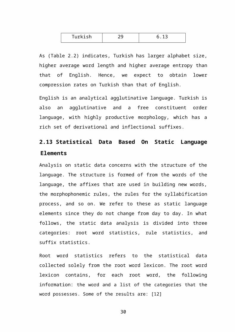
Table 3.3 Letter frequencies in a text file to be compressed

Character Character Frequency

A 29

B 64

C 32

D 12

E 9

F 66

G 23

In practice, the frequencies for all the characters used in the text are needed, including

all letters, digits, and punctuation, but to keep the example simple we'll just stick to the

characters from A to G.

The first step in building a Huffman code is to order the characters from highest to

lowest frequency of occurrence as follows in (Figure 3.2):

Figure 3.2 Ordering characters from highest to lowest frequency

First, the two least-frequent characters are selected, logically grouped together, and their

frequencies added. In this example, the D and E characters have a combined frequency

of 21 as shown down in (Figure 3.3):

Figure 3.3 Combined frequencies of the lowest 2 nodes

66 64 32 29 23 12 9

F B C A G D E

66 64 32 29 23 12 9

F B C A G D E

21

32

This begins the construction of a "binary tree" structure. Again the two elements with

the lowest frequencies are selected, regarding the D-E combination as a single element.

In this case, the two elements selected are G and the D-E combination. They are to be

grouped together and add their frequencies. This new combination will result a new

node has a frequency of 44 as in (Figure 3.4):

Figure 3.4 Combinations of lowest frequency nodes

The same way in selecting the two elements with the lowest frequency, group them

together, and add their frequencies is to be continued, until run out of elements. In the

third iteration, the lowest frequencies are C and A: As shown in (Figure 3.5) the

combination between C and A gives a new node with frequency of 61.

Figure 3.5 Combinations of lowest frequency nodes

66 64 32 29 23 12 9

F B C A G D E

21

44

66 64 32 29 23 12 9

F B C A G D E

21

44

61

33

As we continue by the next iterations combining tow iterations will result a node with

frequency of 105, and another node with frequency of 130. This is shown in the next

two figures, (Figure 3.6) and (Figure 3.7):

Figure 3.6 Combinations between tow nodes

Figure 3.7 Combinations between tow nodes

By the next step which is last step in this example the result is known as a "Huffman

tree". The generated Huffman tree is shown in (Figure 3.8):

66 64 32 29 23 12 9

F B C A G D E

21

44

61

105

66 64 32 29 23 12 9

F B C A G D E

21

44

61

105

130

34

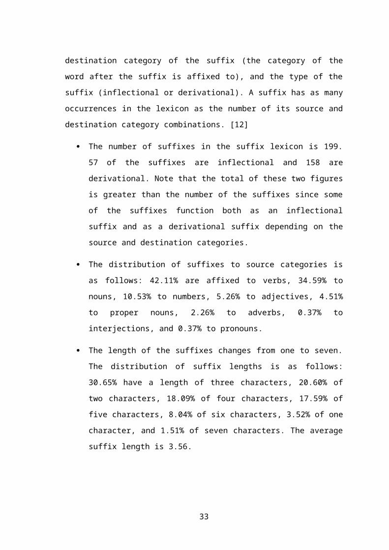
Figure 3.8 Last combination of nodes which result binary Huffman tree

3.4.1.2.7 Obtaining Huffman code from the Tree

To obtain the Huffman code itself, each branch of the tree is labeled with a 1 or 0. It is

important to give 1s for a side and 0s for the other side. Here in this example I will give

0s for the right side and 1s for the left side as shown in (Figure 3.9):

Figure 3.9 Assigning 0s for the right side of the tress and 1s for the left side

66 64 32 29 23 12 9

F B C A G D E

21

44

61

105

130

235

66 64 32 29 23 12 9

F B C A G D E

21

44

61

105

130

235

0

0

0

0

0

10

1

1

1

11

35

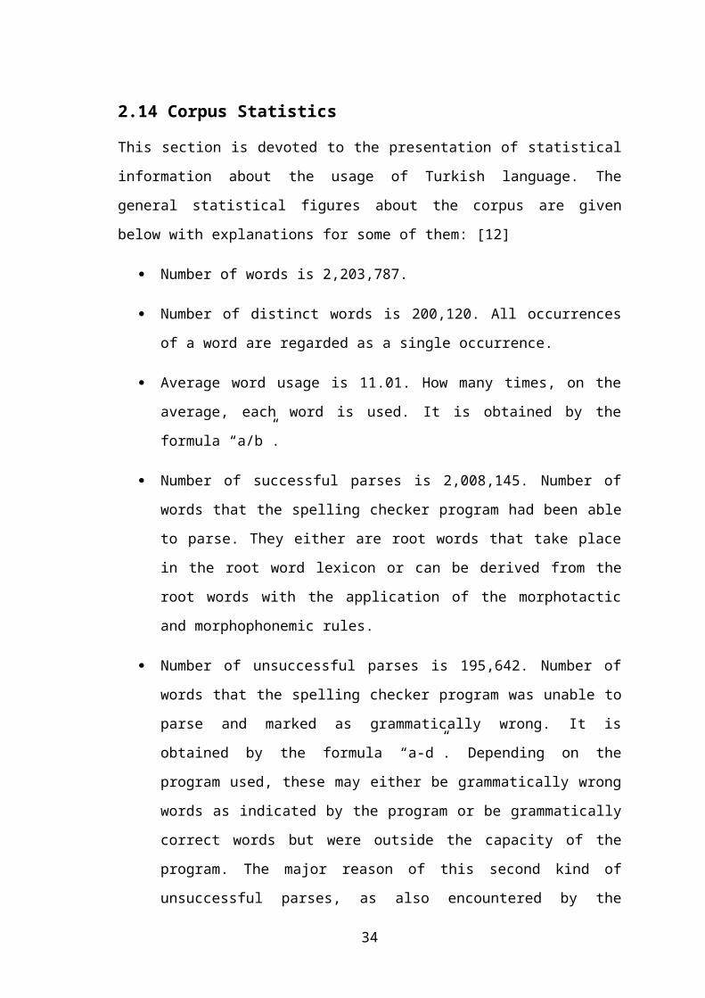
Tracing down the tree gives the "Huffman codes", with the shortest codes assigned to

the characters with the greatest frequency as shown in (Table 3.4) down:

Table 3.4 Original ASCII codes and generated codes for letters in the above example

Character The ASCII code The generated code

F 01000110 00

B 01000010 01

C 01000011 100

A 01000001 101

G 01000111 110

D 01000100 1110

E 01000101 1111

A Huffman coder will go through the source text file, convert each character into its

appropriate binary Huffman code, and dump the resulting bits to the output file. The

Huffman codes won't get mixed up in decoding. The best way to see that this is so is to

envision the decoder cycling through the tree structure, guided by the encoded bits it

reads, moving from top to bottom and then back to the top. As long as bits constitute

legitimate Huffman codes and a bit doesn't get scrambled or lost, the decoder will never

get lost either.

3.4.1.2.8 Advantages and Disadvantages

Huffman compression algorithm is mainly efficient in compressing text or program

files. But it is not very effective if the data in the file is strongly random, since the

frequencies of different characters or bytes would be close to the same, but such

"random" data files are hard to compress by any technique.

36

3.4.2 Dictionary Model Compressor

Dictionary based techniques like LZ-family exploit text redundancy caused by the

grammatical structure of the language text. Generally, they parse the input string into a

sequence of sub strings, or dictionary words, and encode the text by replacing the

parsed token with its dictionary index or with a pointer to its last occurrence in the text.

[14] There are numerous variants that differ in the parsing strategy, the token coding,

and the dictionary update heuristics (for adaptive additions and deletions). The main

characteristic of all of them, and their biggest advantage, is the fact that they are

extremely fast and are therefore very suitable for practical purposes. [24]

3.4.2.1 Lempel Ziv Compression Algorithm

Improvements in the field of data compression up until the late 1970's were chiefly

directed towards creating better methodologies for Huffman Coding. In order to obtain

the necessary frequencies of symbols in the data to be compressed.

In 1977, a new technique was introduced with a very different way of compressing data

- one which would avoid the uncertainty of making predictions or the wastefulness of

pre-reading data and it was know as LZ77 technique.[22] Some new versions of this

technique was described in 1978 and 1984, which was named as LZ78 and LZW

respectively. LZW, which we are interesting in this section, takes that scheme one step

further, actually constructing a "dictionary" of words or parts of words in a message,

and then using pointers to the words in the dictionary.

3.4.2.1.1 History

In 1977, two Israeli information theorists, Abraham Lempel and Jacob Ziv, introduced a

new technique of compressing data was known as "LZ-77", which uses the redundant

nature of text to provide compression. [22]

Lempel and Ziv came up with an improved scheme in 1978, appropriately named "LZ-

78". In 1984, Terry Welch improved LZ78 algorithm, resulting a new version of this

technique named as LZW. The dictionary is the central point of the algorithm.

Furthermore, a hashing technique makes its implementation efficient. LZW

37

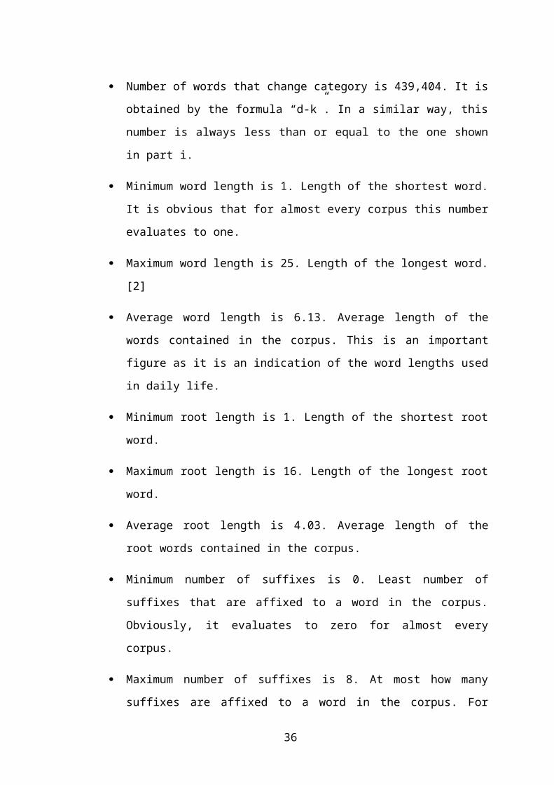
compression was implemented by the "compress" command of the UNIX operating

system.

3.4.2.1.2 LZW CODING

LZ-77 is an example of what is known as "substitutional coding". There are other

schemes in this class of coding algorithms. Lempel and Ziv came up with an improved

scheme in 1978, appropriately named "LZ-78", and it was refined by a Mr. Terry Welch

in 1984, making it "LZW".

LZ-77 uses pointers to previous words or parts of words in a file to obtain compression.

LZW takes that scheme one step further, actually constructing a "dictionary" of words

or parts of words in a message, and then using pointers to the words in the dictionary. [30]

3.4.2.1.3 Description of LZW Algorithm

The key insight of the method is that it is possible to automatically build a dictionary of

previously seen strings in the text being compressed. The dictionary does not have to be

transmitted with the compressed text, since the de-compressor can build it the same way

the compressor does, and if coded correctly, will have exactly the same strings that the

compressor dictionary had at the same point in the text. [18]

The dictionary starts off with 256 entries, one for each possible character (single byte

string). Every time a string not already in the dictionary is seen, a longer string

consisting of that string appended with the single character following it in the text, is

stored in the dictionary.

The output consists of integer indices into the dictionary. These initially are 9 bits each,

and as the dictionary grows, can increase to up to 16 bits. A special symbol is reserved

for "flush the dictionary" which takes the dictionary back to the original 256 entries, and

9 bit indices. This is useful if compressing a text which has variable characteristics,

since a dictionary of early material is not of much use later in the text. [18]

3.4.2.1.4 How Does LZW Compression Algorithm Work

The LZW algorithm stores strings in a "dictionary" with entries for 4,096 variable-

length strings. The first 255 entries are used to contain the values for individual bytes,

so the actual first string index is 256. As the string is compressed, the dictionary is built

38

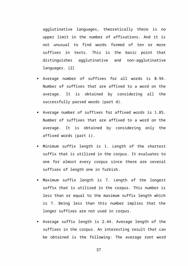
up to contain every possible string combination that can be obtained from the message,

starting with two characters, then three characters, and so on.

Let's use this example message to show how LZW algorithm work, where “_” indicates

the space between the words:

the_rain_in_Spain_falls_mainly_in_the_plain

For example, it is to be scanned through the message to build up dictionary entries as

follows:

256 -> th < th > e_rain_in_Spain_falls_mainly_in_the_plain

257 -> he t < he > _rain_in_Spain_falls_mainly_in_the_plain

258 -> e_ th < e_ > rain_in_Spain_falls_mainly_in_the_plain

259 -> _r the < _r > ain_in_Spain_falls_mainly_in_the_plain

260 -> ra the_ < ra > in_in_Spain_falls_mainly_in_the_plain

261 -> ai the_r < ai > n_in_Spain_falls_mainly_in_the_plain

262 -> in the_ra < in > _in_Spain_falls_mainly_in_the_plain

263 -> n_ the_rai < n_ > in_Spain_falls_mainly_in_the_plain

264 -> _i the_rain < _i > n_Spain_falls_mainly_in_the_plain

The next two-character string in the message is "in", but this has already been included

in the dictionary in entry 262. This means the three-character string "in_” are to be set

up as the next dictionary entry, and then go back to adding two-character strings:

265 -> in_ the_rain_ < in_ > Spain_falls_mainly_in_the_plain

266 -> _S the_rain_in < _S > pain_falls_mainly_in_the_plain

267 -> Sp the_rain_in_ < Sp > ain_falls_mainly_in_the_plain

268 -> pa the_rain_in_S < pa > in_falls_mainly_in_the_plain

The next two-character string is "ai", but that's already in the dictionary at entry 261, so

now a three-character string "ain" is to be added in the next entry:

39

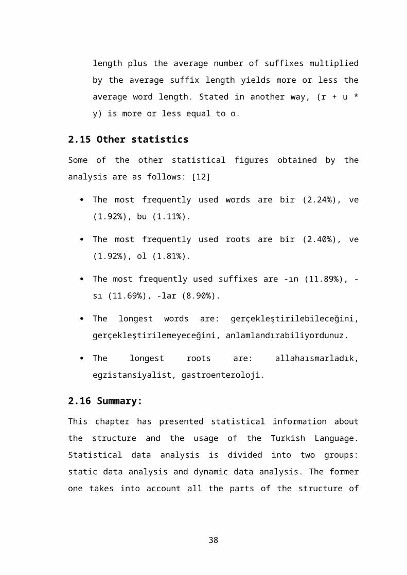
269 -> ain the_rain_in_Sp < ain > _falls_mainly_in_the_plain

Since "n_" is already stored in dictionary entry 263, "n_f" is added as a new dictionary

entry:

270 -> n_f the_rain_in_Spai < n_f > alls_mainly_in_the_plain

271 -> fa the_rain_in_Spain_ < fa > lls_mainly_in_the_plain

272 -> al the_rain_in_Spain_f < al > ls_mainly_in_the_plain

273 -> ll the_rain_in_Spain_fa < ll > s_mainly_in_the_plain

274 -> ls the_rain_in_Spain_fal < ls > _mainly_in_the_plain

275 -> s_ the_rain_in_Spain_fall < s_ > mainly_in_the_plain

276 -> _m the_rain_in_Spain_falls < _m > ainly_in_the_plain

277 -> ma the_rain_in_Spain_falls_ < ma > inly_in_the_plain

Since "ain" is already stored in entry 269, a four-character string "ainl" is stored in the

next dictionary entry:

278 -> ainl the_rain_in_Spain_falls_m < ainl > y_in_the_plain

279 -> ly the_rain_in_Spain_falls_main < ly > _in_the_plain

280 -> y_ the_rain_in_Spain_falls_mainl < y_ > in_the_plain

Since the string "_i" is already stored in entry 264, so an entry is added for the string

"_in":

281 -> _in the_rain_in_Spain_falls_mainly < _in > _the_plain

Since "n_" is already stored in dictionary entry 263, an entry is added for "n_t":

282 -> n_t the_rain_in_Spain_falls_mainly_i < n_t > he_plain

Since "th" is already stored in dictionary entry 256, an entry is added for "the":

283 -> the the_rain_in_Spain_falls_mainly_in_ < the > _plain

Since "e_" is already stored in dictionary entry 258, an entry is added for "e_p":

40

284 -> e_p the_rain_in_Spain_falls_mainly_in_th < e_p > lain

285 -> pl the_rain_in_Spain_falls_mainly_in_the_ < pl > ain

286 -> la the_rain_in_Spain_falls_mainly_in_the_p < la > in

The remaining characters form a string already contained in entry 269, so there is no

need to put it in the dictionary.

So the generated dictionary will contain the strings as shown in (Table 3.5):

Table 3.5 Generated dictionary for the above text

256 -> th 267 -> Sp 278 -> ainl

257 -> he 268 -> pa 279 -> ly

258 -> e_ 269 -> ain 280 -> y_

259 -> _r 270 -> n_f 281 -> _in

260 -> ra 271 -> fa 282 -> n_t

261 -> ai 272 -> al 283 -> the

262 -> in 273 -> ll 284 -> e_p

263 -> n_ 274 -> ls 285 -> pl

264 -> _i 275 -> s_ 286 -> la

265 -> in_ 276 -> _m

266 -> _S 277 -> ma

The dictionary is a means to an end, not an end in itself. The LZW coder simply uses it

as a tool to generate a compressed output. The coder does not output the dictionary to

the compressed output file; the decoder doesn't need it. While the coder is building up

the dictionary, it sends characters to the compressed data output until it hits a string

that's in the dictionary. It outputs an index into the dictionary for that string, and then

continues output of characters until it hits another string in the dictionary, causing it to

output another index, and so on. That means that the compressed output for our example

message looks like this:

the_rain_<262>_Sp<261><263>falls_m<269>ly<264><263><256><258>pl<269>

41

The decoder constructs the dictionary as it reads and uncompresses the compressed

data, building up dictionary entries from the uncompressed characters and dictionary

entries it has already established.

3.4.2.1.5 Decompression

The companion algorithm for compression is the decompression algorithm. It needs to

be able to take the stream of codes output from the compression algorithm, and use

them to exactly recreate the input stream. One reason for the efficiency of the LZW

algorithm is that it does not need to pass the dictionary to the decompression code. The

dictionary can be built exactly as it was during compression, using the input stream as

data. This is possible because the compression algorithm always outputs the STRING

and CHARACTER components of a code before it uses it in the output stream. This

means that the compressed data is not burdened with carrying a large string translation

table (dictionary).

The decompression algorithm is just like the compression algorithm, it adds a new

string to the dictionary each time it reads in a new code. All it needs to do in addition to

that is translate each incoming code into a string and send it to the output.

An important thing to note is that the dictionary ends up looking exactly like the table

built up during compression. The output string is identical to the input string from the

compression algorithm.

3.4.2.1.6 How Does LZW Decompression Algorithm Work

A compressed text is:”/ W E D 256 E 260 261 257 B 260 T” The dictionary would be

created as shown in the following table, (Table 3.6):

Table 3.6 Regenerating dictionary from a compressed file

Input/

NEW_CODEOLD_CODE

STRING/

OutputCHARACTER

New table

entry

/ / /

W / W W 256 = /W

E W E E 257 = WE

D E D D 258 = ED

42

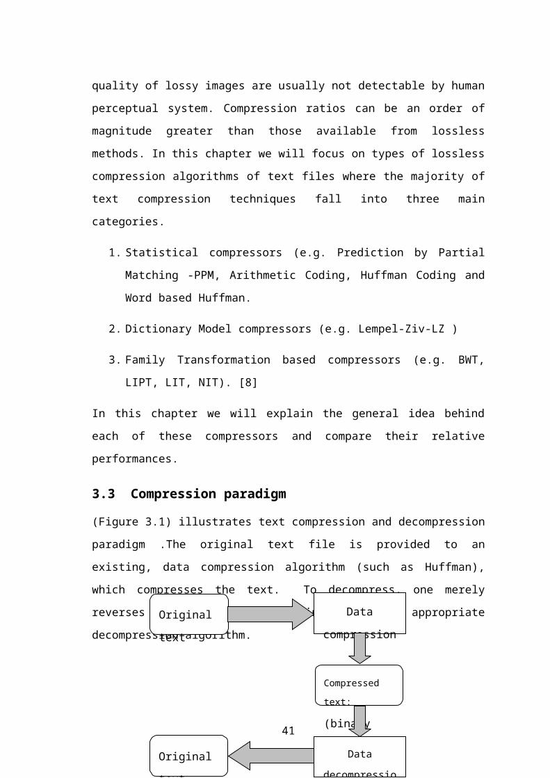
256 D /W / 259 = D/

E 256 E E 260 = /WE

260 E /WE / 261 = E/

261 260 E/ E 262 = /WEE

257 261 WE W 263 = E/W

B 257 B B 264 = WEB

260 B /WE / 265 = B/

T 260 T T 266 = /WET

3.4.2.1.7 Facts about LZW Algorithm

One puzzling thing about LZW is why the first 255 entries in the 4K buffer are

initialized to single-character strings. There would be no point in setting pointers

to single characters, since the pointers would be longer than the characters, and

in practice that's not done anyway. I speculate that the single characters are put

in the buffer just to simplify searching the buffer.

As this example of compressed output shows, as the message is compressed, the

dictionary grows more complete, and the number of "hits" against it increases.

Longer strings are also stored in the dictionary, and on the average the pointers

substitute for longer strings. This means that up to a limit, the longer the

message, the better the compression.

This limit is imposed in the original LZW implementation by the fact that once

the 4K dictionary is complete, no more strings can be added. Defining a larger

dictionary of course results in greater string capacity, but also longer pointers,

reducing compression for messages that don't fill up the dictionary.

A variant of LZW known as "LZC" is used in the old UN*X "compress" data

compression program. LZC uses variable length pointers up to a certain

maximum size. It also monitors the compression of the output stream, and if the

compression ratio goes down, it flushes the dictionary and rebuilds it, on the

assumption that the new dictionary will be better "tuned" to the current text.

43

Another refinement of LZW keep track of string "hits" for each dictionary entry,

and overwrites "least recently used" entries when the dictionary fills up.

Refinements of LZW provide the core of GIF and TIFF image compression as

well.

LZW is also used in some modem communication schemes, such as the

"V.42bis" protocol. V.42bis has an interesting flexibility. Since not all data files

compress well given any particularly encoding algorithm, the V.42bis protocol

monitors the data to see how well it compresses. It sends it "as is" if it

compresses poorly, but will switch to LZW compression using an escape code if

it compresses well. Both the transmitter and receiver continue to build up an

LZW dictionary even while the transmitter is sending the file uncompressed and

switch over transparently if the escape character is sent.

3.4.3 Transformation Based Compression Technique

In mathematics, difficult problems can often be simplified by performing a

transformation on a data set. For example, digital signal processing programs use the

Fast Fourier Transformation (FFT) to convert sets of sampled audio data points to

equivalent sets of frequency data. [7]

Michael Burrows and David Wheeler recently released the details of a transformation

function that opens the door to some revolutionary new data compression techniques.

The Burrows-Wheeler Transform, or BWT, transforms a block of data into a format that

is extremely well suited for compression. [7]

3.4.3.1 History

Michael Burrows and David Wheeler released a research report in 1994 discussing

work they had been doing at the Digital Systems Research Center in Palo Alto,

California. Their paper, "A Block-sorting Lossless Data Compression Algorithm"

presented a data compression algorithm based on a previously unpublished

transformation discovered by Wheeler in 1983. [26]

While the paper discusses a complete set of algorithms for compression and

decompression technique, the real heart of the paper consists of the disclosure of the

BWT algorithm. [7]

44

3.4.3.2 Pre-Compression Transformations

One interesting class of data compression techniques consists of transformation

algorithms. It is often possible to perform a reversible transformation on a data set that

increases its susceptibility to other compression techniques.

The transformations don't compress data at all; they merely prepare the data before

compression is applied. One type of transformation techniques is Burrows-Wheeler

transform (BWT). With BWT transformation technique a good results come from a

three-stage compressor.[8] The output of the BWT transform is usually piped through a

move-to-front (MTF) stage, then a run length encoder (RLE) stage, and finally an

entropy encoder, normally arithmetic or Huffman coding (ARI). The actual command

line to perform this sequence will look something like this: BWT < input-file | MTF |

RLE | ARI > output-file

3.4.3.3 Transformation Based Compress Paradigm

The transformation is designed to make it easier to compress the source file. Paradigm

for transformation compression is illustrated in (Figure 3.10). The original text file is

provided as input to the transformation, which outputs the transformed text. This output

is provided to an existing, unmodified data compression algorithm (such as LZW),

which compresses the transformed text. To decompress, one merely reverses this

process, by first invoking the appropriate decompression algorithm, and then providing

the resulting text to the inverse transform. [4]

Figure 3.10 Text compression paradigm with lossless, reversible transformation.

Data

Decompression

Compressed

text:

(binary code)

Transformed text:

***a^ ** * ***b.

Transform

decoding

Transform

encoding

Original text:

This is a test.

Original text:

This is a test.

Transformed

text:

***a^ ** *

***b.

Data

compression

45

There are several important observations about this paradigm. The transformation must

be exactly reversible, so that the overall lossless text compression paradigm is not

compromised. The data compression and decompression algorithms are unmodified, so

they do not exploit information about the transformation while compressing. The intent

is to use the paradigm to improve the overall compression ratio of the text in

comparison with what could have been achieved by using only the compression

algorithm. An analogous paradigm has been used to compress images and video using

the Fourier transform, Discrete Cosine Transform (DCT) or wavelet transforms

[BGGu98]. In the image/video domains, however, the transforms are usually lossy,

meaning that some data can be lost without compromising the interpretation of the

image by a human. [4]

3.4.3.4 Star-Encoding

Another type of transformation technique is star encoding. While Burrows-Wheeler

transform is a fairly complicated sorting algorithm that radically changes the nature of

an input file. Star-encoding is much simpler to understand.

Star-encoding works by creating a large dictionary of commonly used words expected

in the input files. The dictionary must be prepared in advance, and must be known to the

compressor and de-compressor.

Each word in the dictionary has a star-encoded equivalent, in which as many letters a

possible are replaced by the '*' character. For example, a commonly used word such the

might be replaced by the string t**. The star-encoding transform simply replaces every

occurrence of the word the in the input file with t**.

Ideally, the most common words will have the highest percentage of '*' characters in

their encodings. If done properly, this means that transformed file will have a huge

number of '*' characters. This ought to make the transformed file more compressible

than the original plain text.

3.4.3.4.1 An Example of Star Encoding

But soft, what light through yonder window breaks?

It is the East, and Iuliet is the Sunne,

46

Arise faire Sun and kill the enuious Moone,

Who is already sicke and pale with griefe,

That thou her Maid art far more faire then she

Running this text through the star-encoder yields the following text:

B** *of*, **a* **g** *****g* ***d*r ***do* b*e***?

It *s *** E**t, **d ***i** *s *** *u**e,

A***e **i** *un **d k*** *** e****** M****,

*ho *s a****** **c*e **d **le ***h ****fe,

***t ***u *e* *ai* *r* f*r **r* **i** ***n s**

You can clearly see that the encoded data has exactly the same number of characters,

but is dominated by stars. It certainly looks as though it is more compressible.

3.5 Summary

In this chapter, the most common algorithms for text compression such as Huffman

encoding algorithm, and LZ, lzw algorithm have been described in detail.

In addition, examples are provided for each algorithm which show how the algorithms

work step by step.

47

CHAPTER 4 : DEVELOPMENT OF TEXT COMPRESSION PROGRAM

4.1 Overview

This chapter describes the computer program developed by the author for the

compression of Turkish language text. The chapter shows the interfaces and the

functions of each component of the program. The complete source code of this

application is included in Appendix A.

4.2 The Developed application program

The application program developed by the author has been built to compress text files

of types “*.txt” and “*.doc”. A compressed file is unreadable because the text in the

original file is encoded to new text which is almost rubbish. For this reason a compress

program must have a decompression part that decompresses the encoded file using the

same algorithm. The decompression algorithm can also be used to test the validity and

the correctness of the compression algorithm. Both the compression and the

decompression algorithms are given in this chapter. The application program is based

on the well known encoding algorithm: “Huffman Algorithm”.

As mentioned before in chapter three, Huffman algorithm falls in statistical compressors

category, which use the appearance frequency of characters in compression.

The application developed in this thesis also has a part that shows the frequency of the

characters used in the given text in the form of a graph.

4.3 Turkish alphabets coding:

Unicode's Base Multilingual Plane, which supports almost all languages alphabets, is

used by Windows® operating system. As mentioned in section 2.8 Special Turkish

characters, such as the un-dotted i, appear in the Unicode system within the Latin

Extended-A block (U+0100 – U+017F), which is part of Unicode's Base Multilingual

Plane. The application program works under Windows®, where it will get the benefit of

Turkish alphabet encoding.

48

4.4 The Application algorithm

As mentioned before, the compression is this thesis is based on the Huffman algorithm.

Huffman algorithm’s first step is to consider the frequencies of letters in the file to be

compressed, and sort them decreasing from left to right. The next coming step is the

most important step for Huffman algorithm, which is creating the Huffman tree to get

the new code for the letters. The binary tree (Huffman tree) can easily be constructed by

recursively grouping the lowest frequency characters and nodes, then continuing the

algorithm as described in section 3.4.1.6.2. When some of letter positions were

changed, in some cases better results were obtained.

The method works as Huffman algorithm with a change in building the binary tree.

While in Huffman algorithm the characters are sorted in decreasing way, the method

allows us to change the places of characters in some cases. The time that we have to

change the place of a sorted letter is, if the sum of the new node with the next letter is

smaller than the sum of next letter and the letter after. The letter itself is moved to the

right of the tree.

The algorithm is as follows:

1. Sort all characters decreasingly according to letter frequency and initially are

considered as free nodes.

2. The two free nodes with the lowest frequency are assigned to a parent node with

a weight equal to the sum of the two child nodes.

3. If sum of (new node + next node) < (next node+ the node after) move the next

node to the right of the tree.

4. Steps 2 through 3 are repeated until there is only one free node left. This free

node is the root of the tree.

Getting the code from the tree

To see the code, redraw all the symbols in the form of a tree, where each symbol

contains either a single letter or splits up into two smaller symbols.

5. Label all the left branches of the tree with a 0 and all the right branches with a 1.

The code for each of the letters is the sequence of 0's and 1's that lead to it on the

tree, starting from the head of the tree.

49

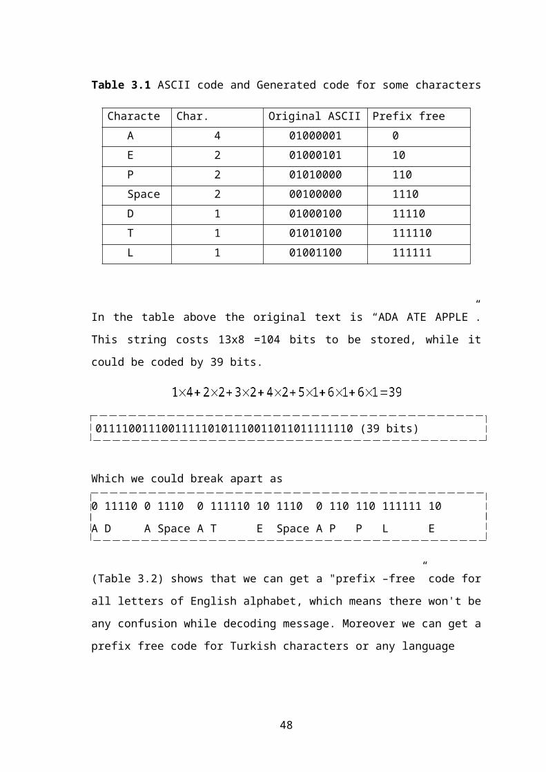
Figure 4.1 Flowchart of the application algorithm.

4.5 Two Examples:

Here in this section two examples will be shown applying compression using the

original Huffman method and the other method. These two examples will show that

Start

Sort Character Frequency Decreasingly

Sum the Least 2 nodes

Label Left Branch with 0 & Right with 1

Is This the

Root Node

Collect Bits Starting

From the Root

Reaching Each Letter

Stop

(new node+ next node)<

(next node+ the node after)

is

Move next node to

right

50

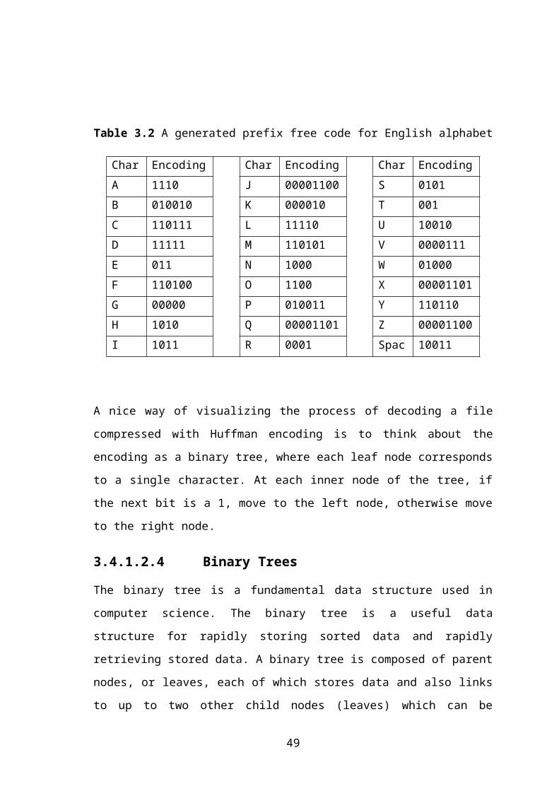
moving some characters to the right of the tree will be either better or the same without

moving, but it will not be worst. (Figure 4.2) and (Figure 4.3) shows the situation where

results where obtained in both cases.

(a) (b)

Figure 4.2 creating a binary tree, (a) without moving, (b) with moving characters.

(Figure 4.1) shows that it remains same compression result if some letter position were

moved or not. Where compression results in both cases will be 445 bytes in both cases,

where the original text size is1400 bytes.

(a) (b)

Figure 4.3 creating a binary tree, (a) without moving, (b) with moving characters.

But (Figure 4.2) shows that letters moving case results better compression result. While

the original size is 464 bytes, while the compression results in both cases is 153 bytes

without moving and 131 bytes with letter possession moving.

As creating binary tree moving characters possession causes some letters that have high

frequency to flout to the top of the binary tree. The letters those on the top of the tree

take less bits to coded. That is why better compression results could be gained.

51

4.6 The User application Interface

The user interface of the application developed in this thesis consists of one simple

window. This window contains some buttons, text bars and other tools. Using these

tools we will be able to compress and decompress text files and get some information

about the characteristics of the compressed file. (Figure 4.4) shows the application

interface which will be described in more detail within this chapter.

Figure 4.4 User interface of the application developed by the author

4.7 Software Development language

Visual Basic 6.0 programming language was used in developing the application

program in this thesis. The application program will be described in this chapter.

4.7.1 Why Visual Basic 6.0?

There are many reasons for choosing Visual Basic over other tools; among them are the

following:

A comprehensive object framework.

A fast, native-code compiler.

A development environment based on sophisticated two-way tools.

52

Compatible with Microsoft Windows 9x, Windows ME, Windows 2000,

Windows XP and Linux.

Visual Basic took all the best elements of modern Windows development tools

and wove them into a single product.

You can drop components onto a form to build almost any type of application.

You can generate normal Windows EXEs with the press of a key.

Supports direct access to the Windows API.

Make it easy to create DLLs and other secondary Windows objects.

Get benefit of using object-oriented that include Inheritance, Polymorphism,

Encapsulation and Primary Methodology, which is full used in Visual Basic net

VB.net.

4.8 Parts of the program listing

The complete source code of the application program is given in Appendix A. In this

section, only the important parts of the source code, namely the creation of the Huffman

binary tree is discussed.

Public Sub DecodeFile(SourceFile As String, DestFile As String) Dim ByteArray() As Byte Dim Filenr As Integer 'Make sure the source file exists If (Not FileExist(SourceFile)) Then Err.Raise vbObjectError, "clsHuffman.DecodeFile()", "Source file does not exist" End If 'Read the data from the sourcefile Filenr = FreeFile Open SourceFile For Binary As #Filenr ReDim ByteArray(0 To LOF(Filenr) - 1) Get #Filenr, , ByteArray() Close #Filenr 'Uncompress the data Call DecodeByte(ByteArray(), UBound(ByteArray) + 1) 'If the destination file exist we need to 'destroy it because opening it as binary

53

'will not clear the old data If (FileExist(DestFile)) Then Kill DestFile 'Save the destination string Open DestFile For Binary As #Filenr Put #Filenr, , ByteArray() Close #Filenr

End Sub

Private Sub CreateTree(Nodes() As HUFFMANTREE, NodesCount As Long, Char As Long, Bytes As ByteArray) Dim a As Integer Dim NodeIndex As Long NodeIndex = 0

For a = 0 To (Bytes.Count - 1) If (Bytes.Data(a) = 0) Then 'Left node If (Nodes(NodeIndex).LeftNode = -1) Then Nodes(NodeIndex).LeftNode = NodesCount Nodes(NodesCount).ParentNode = NodeIndex Nodes(NodesCount).LeftNode = -1 Nodes(NodesCount).RightNode = -1 Nodes(NodesCount).Value = -1 NodesCount = NodesCount + 1 End If

NodeIndex = Nodes(NodeIndex).LeftNode ElseIf (Bytes.Data(a) = 1) Then 'Right node If (Nodes(NodeIndex).RightNode = -1) Then Nodes(NodeIndex).RightNode = NodesCount Nodes(NodesCount).ParentNode = NodeIndex Nodes(NodesCount).LeftNode = -1 Nodes(NodesCount).RightNode = -1 Nodes(NodesCount).Value = -1 NodesCount = NodesCount + 1 End If NodeIndex = Nodes(NodeIndex).RightNode Else Stop End If Next Nodes(NodeIndex).Value = CharEnd Sub

54

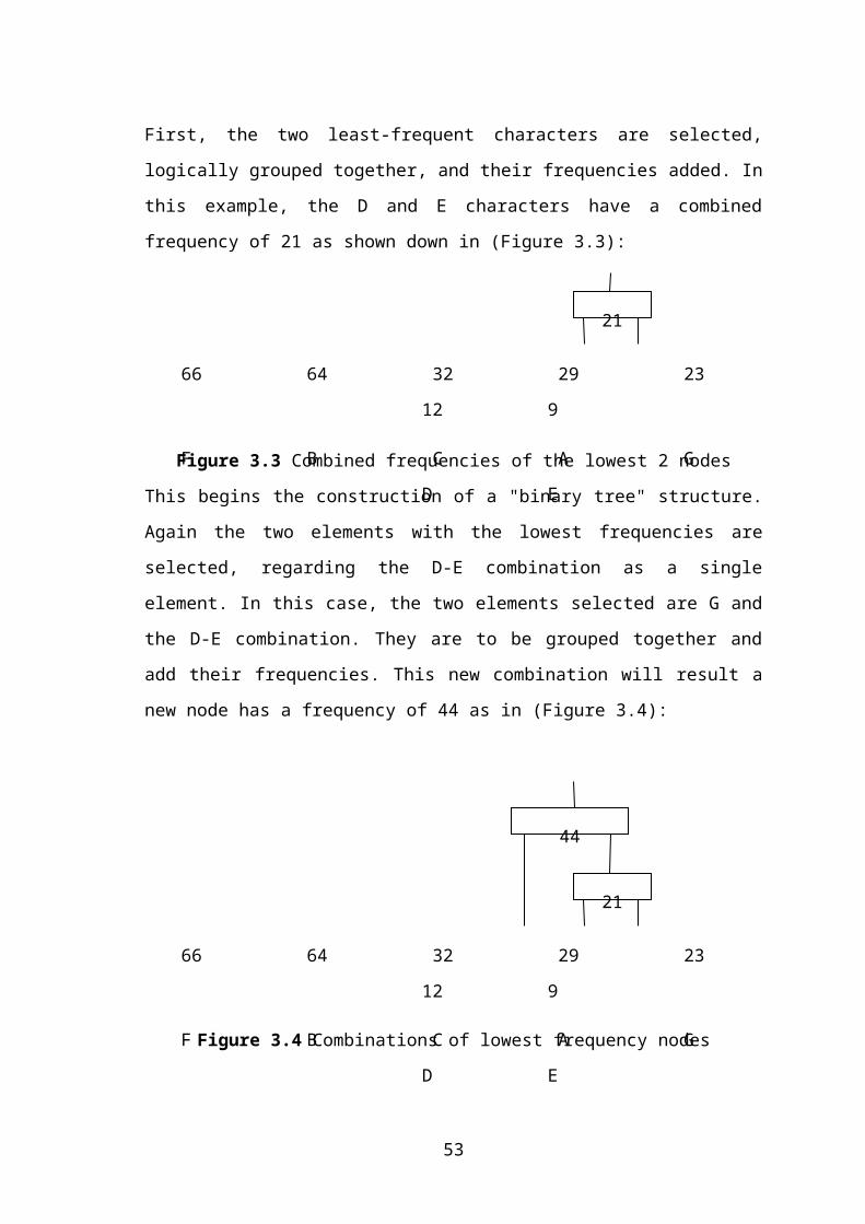
4.9 . Functions of the application program interfaces

When the application program is run, the user interface shown in (Figure 4.2) is

obtained. On the application interface window the following tools exist:

1. Two Radio buttons to activate the function we are going to apply.

2. Six command buttons to give the order we are going to apply.

3. Four text boxes tools to get the file name and path for files are going to be

compressed or decompressed.

4. One text list to get the frequency of letters in the file to be compressed.

5. One Graph to show the frequency of letters in graphical way.

6. Some information labels to give information about the file being compressed.

On the following sections I am going to explain these tools and there functions.

4.9.1 Radio Buttons

These are used to activate the part we are going to apply of the program. Compress

radio button will activate the compress part. As well as the decompress radio will

activate the decompress part of the program. (Figure 4.5) shows that compress part of

the program is active while the decompress pat is non-active. While when selecting the

decompress radio button the decompress part is activated as in (Figure 4.6).

Figure 4.5 Activating the compress part of the program

55

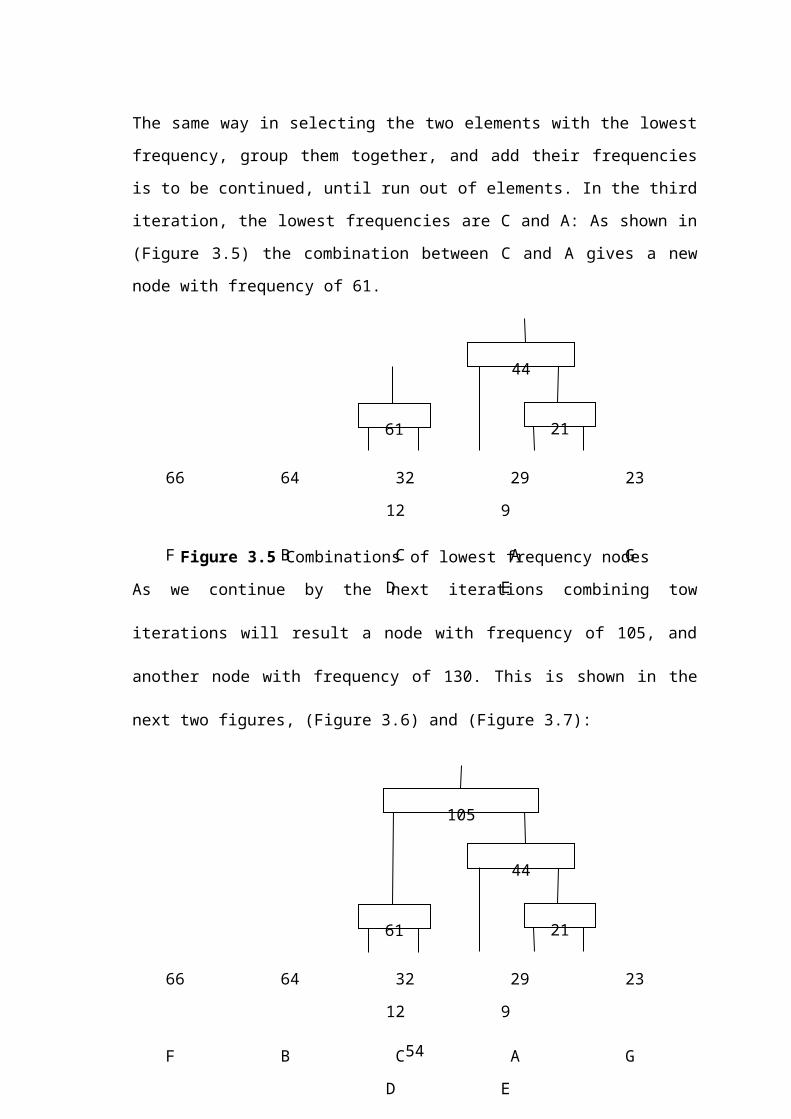
Figure 4.6 Activating the de-compress part of the program

4.9.2 Command buttons

On the interface window we have six command buttons each one have its function as

follows:

Brows Buttons: each of them is used to help the user for finding the file is going to be

compressed, while it opens the open window.

Compress Button: after selecting the file to be compressed, we press on this button to

apply the compress function and get the new compressed file which name and path is

written on the second text box.

Decompress Button: will apply the decompress function on a compressed file secreted

on the “File to be compressed” text button.

Frequency Button: shows the letter frequencies in the file being compressed by

numbers on the list text box and by graph on the “Frequency Graph” part.

Close Button: to end working on the application program.

4.9.3 Text boxes

As shown in (Figure 4.7) we have four text boxes on my program only two of them are

active at a time.

56

Figure 4.7 Text boxes used on the program

Source file: will contain the name and path of the original file is being compressed.

Compressed File (HUF): contains the path and file name of the new file (compressed

file) while extension of the original file will be changed from (*.txt) to (*.huf).

File to be decompressed and Decompress to file: will be active together when

selecting the decompress radio button. These are used to help the user to decompress a

compressed file, while they will contain the compressed file name and destination and

the new file name and destination respectively.

4.9.4 Text list

Will contain each letter presented in the file being compressed as a list, and will show

the letters frequencies. Text list is shown in (Figure 4.8):

Figure 4.8 The text list used to display the letter frequency of the project

57

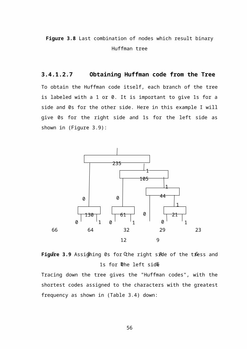
4.9.5 Graph tool

(Figure 4.9) shows the frequency of each letter of the file being compressed in graphical

way, to make it easy for the user to read the frequency. In the following example

characters “a” and “i” have the highest frequencies.

Figure 4.9 Letter frequencies shown in graphical shape

4.10 Summary

This chapter has described the application program developed by the author. The user

interface has also been described in detail. The presented graphical user interface and

the functions carried out when using the buttons, were developed using Visual Basic 6.0

programming language.

58

CHAPTER 5 : RESULTS OF SIMULATION

5.1 Overview

This chapter shows the results of using program to compress files with different sizes.

Two types of text files were tried: “*.txt” and “*.doc” files.

5.2 Files to be compressed

Changing the type of file will change the size, because each type has its characteristics

like the file header etc. So I preferred to apply the developed compression program on

two types of files. 7 files of types “.DOC”, and 7 files of types “.TXT” have been tested

using the program. The sizes of these files are given in (Table 5.1).

Table 5.1 Original file sizes tested using the program

Document Files

(*.Doc)

Size on Disk

In Bytes

Text Files

(*.txt)

Size on Disk

In Bytes

1.Doc 21504 1t.Txt 1854

2.Doc 34304 2t.Txt 14544

3.Doc 62464 3t.Txt 35912

4.Doc 128000 4t.Txt 90788

5.Doc 248832 5t.Txt 196264

6.Doc 437760 6t.Txt 360966

7.Doc 523264 7t.Txt 404778

5.3 Compressing a file

Compressing a file will produce a new file of type which I suggested to be Huf (*.Huf).

The new files can be opened by notepad program but they are not readable by the user.

Here, a small file is shown before and after compression.

5.3.1 Original text file

PVC NEDİR?

PVC, yaygın deyimi ile "vinil" , (Poli Vinil Klorür) kelimesinin kısaltılmış şeklidir ve

petrol (veya doğalgaz) ile tuz'dan petrokimya tesislerinde üretilen, formülü - (CH2-

59

CH2) olan bir polimer türüdür. Bu polimer, çeşitli katkı maddeleri ile harmanlandıktan

sonra yüksek sıcaklıklarda şekillendirilerek plastik haline getirilir ve kullanılır. PVC,

polimer zincirinde klor atomu taşıyan ender termoplastiklerdendir. Klor içermesi nedeni

ile PVC'nin alev alma sıcaklığı yüksektir, alev tutuştuğunda kendiliğinden hemen söner.

PVC çok yüksek sıcaklarda termal olarak kolaylıkla bozulur ve korrozif bir gaz olan

hidroklorik asit çıkarır. PVC, diğer polimerlere kıyasla daha fazla miktarda ve çeşitte

katkı maddesi ile karıştırılabilir. Bu nedenle de, PVC plastik malzemenin maliyeti

nispeten düşüktür; genel ve çok amaçlı kullanım sağlar. PVC, Polietilen'i takiben en çok

kullanılan bir polimer türüdür.

5.3.2 File after compression

Figure 5.1 shows the above text after compression which is unreadable text, because a

new code will be generated for it to be compressed. I used notepad program to open the

generated file.

Figure 5.1 An example of file after compression

5.4 Applying compression using the program

As it is mentioned before, 14 files were used in the compression test. In (Table 5.2), the

results of applying the compression to 7 of the “*.Doc” type files is given. The results

table contains the original file sizes, the new file sizes and the compression ratios. Table

5.3 shows the results of applying the compression to other 7 files which are of type

“*.txt”.

60

Table 5.2 Result of applying the compression program on Doc files

File name Old file size

In Bytes

New file size

In Bytes

Comp. ratio

1.Doc 21504 5988 72%

2.Doc 34304 12902 62%

3.Doc 62464 26254 57%

4.Doc 128000 58144 54%

5.Doc 248832 112506 54%

6.Doc 437760 198931 54%

7.Doc 523264 248693 52%

Table 5.3 Result of applying the compression program on txt files

File name Old file size

In Bytes

New file size

In Bytes

Comp. ratio

1t.txt 1854 988 46%

2t.txt 14544 6699 53%

3t.txt 39512 17625 55%

4t.txt 90788 40129 55%

5t.txt 196264 86566 55%

6t.txt 360966 158891 55%

7t.txt 404778 178298 55%

61

5.5 Summary

In this chapter the results of using the program to compress various files have been

shown. 7 files of type “.doc” and 7 files of type “.txt” have been used in the test. On

average, the compression ratio for the “.doc” files was 58%, and the compression ratio

for the “.txt” files was 53%.

62

CONCLUSION

Data compression is a vast field and is very useful in computing world especially in

networking and data storage. Data compression could be realized through many

methods. For text data compression, lossless compression algorithms must be applied to

avoid losing even a single character from the text.

Huffman algorithm is one of the efficient methods which have been successfully

applied in the field of text data compression. This thesis focused on text compression

especially Turkish language text compression using a statistical algorithm, which is

Huffman encoding algorithm. In compressing Turkish language text we must consider

that it has characters not included in the standard ASCII table. For this thesis an

algorithm and a computer program that compress text files was developed. The program

applied on totally unconstrained computerized Turkish text files.

This thesis consists of five chapters. Chapter one explained the importance and a brief

history of developing data compression. Moreover it described the classifications of

data compression. Statistical information about the structure and the usage of Turkish

Language was presented in chapter two. In chapter three, the most common algorithms

for text compression such as Huffman encoding algorithm, LZ, lzw algorithm was

explained with examples. Chapter four describes the application program developed for

this thesis. Results of Turkish text files compression using the developed system was

shown in chapter five and it was more than 50% compressed data. The developed

program was applied on 14 files, were 7 of these files were of type “.doc”, and 7 were

of type “.txt”. On average, the compression ratio for “.doc” files was 58%, and the

compression ratio for “.txt” files was 53%.

63

REFERENCES

1. Aysan Bayramoğlu, Let’s Learn Turkish 2nd Edition,Gelişim offset, Lefkoşa 1991.

2. Dalkiliç, G., and Çebi Y., 2004, “Word Statistics of Turkish Language on a Large

Scale Text Corpus - TurCo”, ITCC 2004, IEEE International Conference on

Information Technology, Vol:2, pp. 319-325.

3. E. CELIKEL, B. DINCER, Improving the Compression Performance of Turkish

Texts with PoS Tags., International Conference on Information and Knowledge

Engineering (IKE’04).

4. F Robert,K Holger, Z Nan,I Raja, and M Amar, Lossless, Reversible Transformations

that Improve Text Compression Ratios, University of Central Florida.

5. F. Çuna Ekmekçioglu, Michael F. Lynch, and Peter Willett, Stemming and N-gram

matching for term conflation in Turkish texts, Information Research, Vol. 2 No. 2,

October 1996.

6. James D. Murray and William vanRyper, Encyclopedia of Graphics File Formats,

Second Edition, 1996.

7. Mark Nelson, Data Compression with the Burrows-Wheeler Transform, Dr. Dobb's

Journal September, 1996 .

8. Mark Nelson, Star-Encoding in C++, Dr. Dobb's Journal August, 2002.

9. Meeting with Prof. Dr. Bülent YORULMAZ, Dean of Fen-Edebiyat Fakültesi NEU,

chairman of Turkish language and literature department.

10. Steven Atkin & Alihan Irmakkesen , Computing in Turkish.

11. Steven W. Smith, The Scientist and Engineer's Guide to Digital Signal Processing,

Second Edition, 1999.

12. T. Güngör Lexical and Morphological Statistics For Turkish, International XII.

Turkish Symposium on Artificial Intelligence and Neural Networks - TAINN 2003.

13. T. Güngör, Computer Processing of Turkish: Morphological and Lexical

Investigation, Ph.D. Dissertation, Boğaziçi University, İstanbul, 1995.

14. Terry A. Welch. “A Technique for High Performance Data Compression”. IEEE

Computer, Vol. 17, No. 6, 1984, pp. 8-19.

Internet References:

15. http://computing-dictionary.thefreedictionary.com/Huffman+tree

16. http://en.wikipedia.org/wiki/Huffman_tree

17. http://scic.cec.eu.int/Main/enlargement/lan_pres/turk_01.htm

64

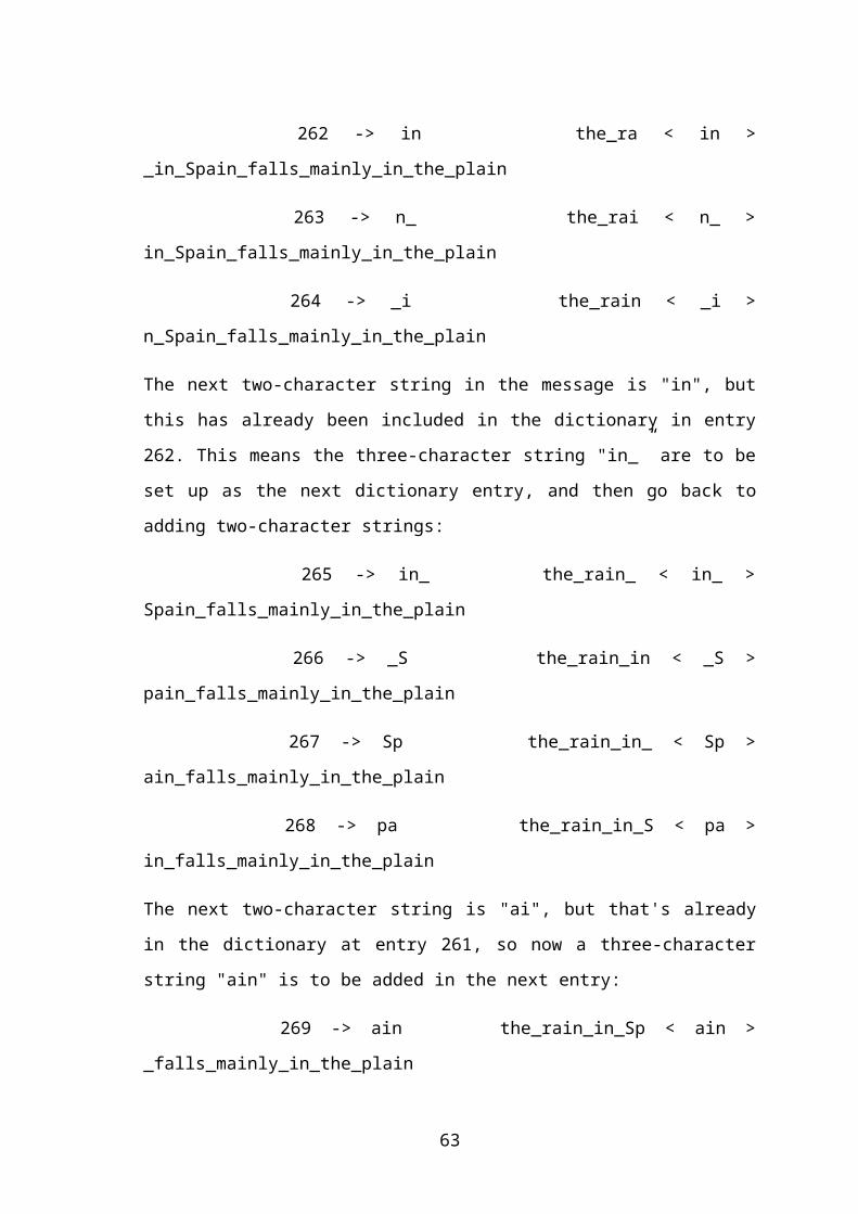
18. http://www.answers.com/topic/lzw-1

19. http://www.array.com/compres.pdf

20. http://www.cprogramming.com/tutorial/computersciencetheory/huffman.html

21. http://www.cprogramming.com/tutorial/lesson18.html

22. http://www.cs.mcgill.ca/~cs251/OldCourses/1997/topic23/

23. http://www.cs.sfu.ca/cs/CC/365/li/squeeze/AdaptiveHuff.html

24. http://www.cs.ucf.edu/~nmotgi/thesisproposal.html

25. http://www.data-compression.com/index.shtml

26. http://www.data-compression.info/Algorithms/BWT/

27. http://www.eee.bham.ac.uk/WoolleySI/All7/main.htm

28. http://www.livejournal.com/users/parakleta/137282.html

29. http://www.transparent.com/languagepages/turkish/overview.htm

30. http://www.vectorsite.net/ttdcmp1.html

31. http://www.wolframscience.com/reference/notes/1069b

65

APPENDIX A: LISTING OF SOURCE CODE

1

APPENDIX B: ENGLISH LANGUAGE ALPHABETS

1

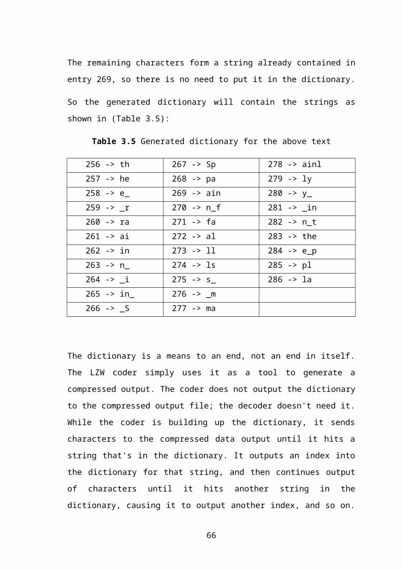
APPENDIX C: TURKISH LANGUAGE ALPHABETS

1