introduction - monash universityusers.monash.edu/~jpurcell/papers/weaving-2016.pdf · weaving knots...

VOLUME BOUNDS FOR WEAVING KNOTS

ABHIJIT CHAMPANERKAR, ILYA KOFMAN, AND JESSICA S. PURCELL

Abstract. Weaving knots are alternating knots with the same projection as torus knots,and were conjectured by X.-S. Lin to be among the maximum volume knots for fixed crossingnumber. We provide the first asymptotically sharp volume bounds for weaving knots, andwe prove that the infinite square weave is their geometric limit.

1. Introduction

The crossing number, or minimum number of crossings among all diagrams of a knot, isone of the oldest knot invariants, and has been used to study knots since the 19th century.Since the 1980s, hyperbolic volume has also been used to study and distinguish knots. Weare interested in the relationship between volume and crossing number. On the one hand, itis very easy to construct sequences of knots with crossing number approaching infinity butbounded volume. For example, start with a reduced alternating diagram of an alternatingknot, and add crossings by twisting two strands in a fixed twist region of the diagram. Bywork of Jørgensen and Thurston, the volume of the resulting sequence of knots is boundedby the volume of the link obtained by augmenting the twist region (see [27, page 120]).However, since reduced alternating diagrams realize the crossing number (see for example[26]), the crossing number increases with the number of crossings in the twist region.

On the other hand, since there are only a finite number of knots with bounded crossingnumber, among all such knots there must be one (or more) with maximal volume. It is anopen problem to determine the maximal volume of all knots with bounded crossing number,and to find the knots that realize the maximal volume per crossing number.

In this paper, we study a class of knots and links that are candidates for those with thelargest volume per crossing number: weaving knots. For these knots and links, we provideexplicit, asymptotically sharp bounds on their volumes. We also prove that they convergegeometrically to an infinite link complement which asymptotically maximizes volume percrossing number. Thus, while our methods cannot answer the question of which knotsmaximize volume per crossing number, they provide evidence that weaving knots are amongthose with largest volume once the crossing number is bounded.

A weaving knot W (p, q) is the alternating knot or link with the same projection as thestandard p–braid (σ1 . . . σp−1)

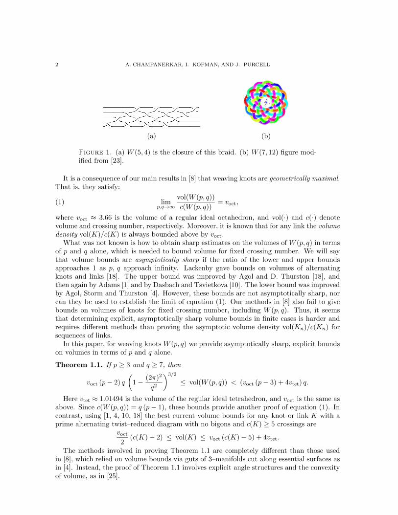
q projection of the torus knot or link T (p, q). Thus, the crossingnumber c(W (p, q)) = q(p − 1). For example, W (5, 4) and W (7, 12) are shown in Figure 1.By our definition, weaving knots can include links with many components, and throughoutthis paper, weaving knots will denote both knots and links.

Xiao-Song Lin suggested in the early 2000s that weaving knots would be among the knotswith largest volume for fixed crossing number. In fact, we checked thatW (5, 4) has the secondlargest volume among all 1, 701, 936 prime knots with c(K) ≤ 16 (good guess!). These knotswere classified by Hoste, Thistlethwaite, and Weeks [17], and are available for further study,including volume computation, in the Knotscape [16] census, or via SnapPy [9].

1

2 A. CHAMPANERKAR, I. KOFMAN, AND J. PURCELL

(a) (b)

Figure 1. (a) W (5, 4) is the closure of this braid. (b) W (7, 12) figure mod-ified from [23].

It is a consequence of our main results in [8] that weaving knots are geometrically maximal.That is, they satisfy:

(1) limp,q→∞

vol(W (p, q))

c(W (p, q))= voct,

where voct ≈ 3.66 is the volume of a regular ideal octahedron, and vol(·) and c(·) denotevolume and crossing number, respectively. Moreover, it is known that for any link the volumedensity vol(K)/c(K) is always bounded above by voct.

What was not known is how to obtain sharp estimates on the volumes of W (p, q) in termsof p and q alone, which is needed to bound volume for fixed crossing number. We will saythat volume bounds are asymptotically sharp if the ratio of the lower and upper boundsapproaches 1 as p, q approach infinity. Lackenby gave bounds on volumes of alternatingknots and links [18]. The upper bound was improved by Agol and D. Thurston [18], andthen again by Adams [1] and by Dasbach and Tsvietkova [10]. The lower bound was improvedby Agol, Storm and Thurston [4]. However, these bounds are not asymptotically sharp, norcan they be used to establish the limit of equation (1). Our methods in [8] also fail to givebounds on volumes of knots for fixed crossing number, including W (p, q). Thus, it seemsthat determining explicit, asymptotically sharp volume bounds in finite cases is harder andrequires different methods than proving the asymptotic volume density vol(Kn)/c(Kn) forsequences of links.

In this paper, for weaving knots W (p, q) we provide asymptotically sharp, explicit boundson volumes in terms of p and q alone.

Theorem 1.1. If p ≥ 3 and q ≥ 7, then

voct (p− 2) q

(1− (2π)2

q2

)3/2

≤ vol(W (p, q)) < (voct (p− 3) + 4vtet) q.

Here vtet ≈ 1.01494 is the volume of the regular ideal tetrahedron, and voct is the same asabove. Since c(W (p, q)) = q (p− 1), these bounds provide another proof of equation (1). Incontrast, using [1, 4, 10, 18] the best current volume bounds for any knot or link K with aprime alternating twist–reduced diagram with no bigons and c(K) ≥ 5 crossings are

voct2

(c(K)− 2) ≤ vol(K) ≤ voct (c(K)− 5) + 4vtet.

The methods involved in proving Theorem 1.1 are completely different than those usedin [8], which relied on volume bounds via guts of 3–manifolds cut along essential surfaces asin [4]. Instead, the proof of Theorem 1.1 involves explicit angle structures and the convexityof volume, as in [25].

VOLUME BOUNDS FOR WEAVING KNOTS 3

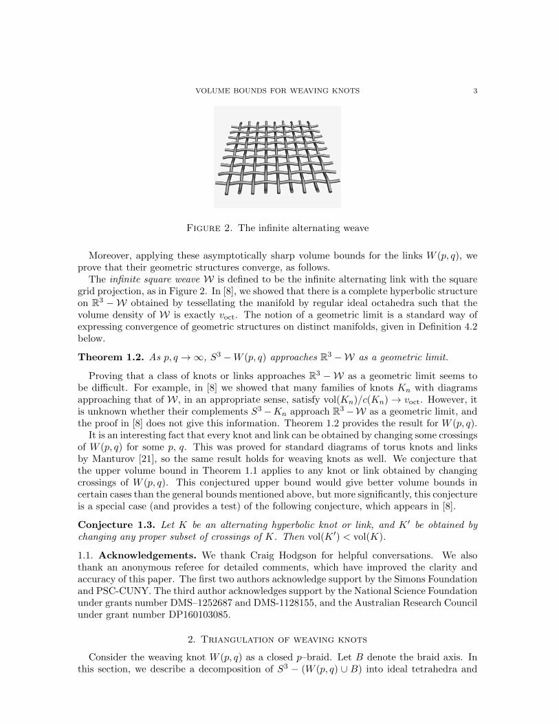
Figure 2. The infinite alternating weave

Moreover, applying these asymptotically sharp volume bounds for the links W (p, q), weprove that their geometric structures converge, as follows.

The infinite square weave W is defined to be the infinite alternating link with the squaregrid projection, as in Figure 2. In [8], we showed that there is a complete hyperbolic structureon R3 −W obtained by tessellating the manifold by regular ideal octahedra such that thevolume density of W is exactly voct. The notion of a geometric limit is a standard way ofexpressing convergence of geometric structures on distinct manifolds, given in Definition 4.2below.

Theorem 1.2. As p, q →∞, S3 −W (p, q) approaches R3 −W as a geometric limit.

Proving that a class of knots or links approaches R3 −W as a geometric limit seems tobe difficult. For example, in [8] we showed that many families of knots Kn with diagramsapproaching that of W, in an appropriate sense, satisfy vol(Kn)/c(Kn)→ voct. However, itis unknown whether their complements S3−Kn approach R3−W as a geometric limit, andthe proof in [8] does not give this information. Theorem 1.2 provides the result for W (p, q).

It is an interesting fact that every knot and link can be obtained by changing some crossingsof W (p, q) for some p, q. This was proved for standard diagrams of torus knots and linksby Manturov [21], so the same result holds for weaving knots as well. We conjecture thatthe upper volume bound in Theorem 1.1 applies to any knot or link obtained by changingcrossings of W (p, q). This conjectured upper bound would give better volume bounds incertain cases than the general bounds mentioned above, but more significantly, this conjectureis a special case (and provides a test) of the following conjecture, which appears in [8].

Conjecture 1.3. Let K be an alternating hyperbolic knot or link, and K ′ be obtained bychanging any proper subset of crossings of K. Then vol(K ′) < vol(K).

1.1. Acknowledgements. We thank Craig Hodgson for helpful conversations. We alsothank an anonymous referee for detailed comments, which have improved the clarity andaccuracy of this paper. The first two authors acknowledge support by the Simons Foundationand PSC-CUNY. The third author acknowledges support by the National Science Foundationunder grants number DMS–1252687 and DMS-1128155, and the Australian Research Councilunder grant number DP160103085.

2. Triangulation of weaving knots

Consider the weaving knot W (p, q) as a closed p–braid. Let B denote the braid axis. Inthis section, we describe a decomposition of S3 − (W (p, q) ∪ B) into ideal tetrahedra and


Figure 3. Polygonal decomposition of cusp corresponding to braid axis. Afundamental region consists of four triangles and 2(p−3) quads. The exampleshown here is p = 5. The black diagonal is the preimage of a meridian.

��

��

��

��

Figure 4. Left: Dividing projection plane into triangles and quadrilaterals.Right: Coning to ideal octahedra and tetrahedra, figure modified from [19].

octahedra. This leads to our upper bound on volume, obtained in this section. In Section 3we will use this decomposition to prove the lower bound as well.

Let p ≥ 3. Note that the complement of W (p, q) in S3 with the braid axis also removedis a q–fold cover of the complement of W (p, 1) and its braid axis.

Lemma 2.1. Let B denote the braid axis of W (p, 1). Then S3 − (W (p, 1) ∪ B) admits anideal polyhedral decomposition P with four ideal tetrahedra and p− 3 ideal octahedra.

Moreover, a meridian for the braid axis runs over exactly one side of one of the idealtetrahedra. The polyhedra give a polygonal decomposition of the boundary of a horoball neigh-borhood of the braid axis, with a fundamental region consisting of four triangles and 2(p− 3)quadrilaterals, as shown in Figure 3.

Proof. Consider the standard diagram of W (p, 1) in a projection plane, which B intersectsin two points. Obtain an ideal polyhedral decomposition as follows. First, for every crossingof the W (p, 1) diagram, take an ideal edge, the crossing arc, running from the knot strandat the top of the crossing to the knot strand at the bottom. This subdivides the projectionplane into two triangles and p − 3 quadrilaterals that correspond to the regions of the linkprojection. This is shown in Figure 4 (left) when p = 5. In the figure, note that the fourdotted red edges shown at each crossing are homotopic to the crossing arc.

Now for each quadrilateral on the projection plane, add four edges between ideal verticesabove the projection plane and four below, as follows. Those edges above the projection planerun vertically from the strand of W (p, 1) corresponding to an ideal vertex of the quadrilateralto the braid axis B. Those edges below the projection plane also run from strands of W (p, 1)corresponding to ideal vertices of the quadrilateral, only now they run below the projectionplane to B. These edges bound eight triangles, as follows. Four of the triangles lie above theprojection plane, with two sides running from a strand of W (p, 1) to B and the third in theprojection plane, connecting two vertices of the quadrilateral. The other four lie below, againeach with two edges running from strands of W (p, 1) to B and one edge on the quadrilateral.


2

T2

11

T

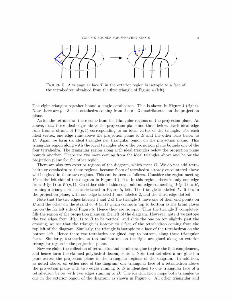
Figure 5. A triangular face T in the exterior region is isotopic to a face ofthe tetrahedron obtained from the first triangle of Figure 4 (left).

The eight triangles together bound a single octahedron. This is shown in Figure 4 (right).Note there are p− 3 such octahedra coming from the p− 3 quadrilaterals on the projectionplane.

As for the tetrahedra, these come from the triangular regions on the projection plane. Asabove, draw three ideal edges above the projection plane and three below. Each ideal edgeruns from a strand of W (p, 1) corresponding to an ideal vertex of the triangle. For eachideal vertex, one edge runs above the projection plane to B and the other runs below toB. Again we form six ideal triangles per triangular region on the projection plane. Thistriangular region along with the ideal triangles above the projection plane bounds one of thefour tetrahedra. The triangular region along with ideal triangles below the projection planebounds another. There are two more coming from the ideal triangles above and below theprojection plane for the other region.

There are also two exterior regions of the diagram, which meet B. We do not add tetra-hedra or octahedra to these regions, because faces of tetrahedra already encountered abovewill be glued in these two regions. This can be seen as follows. Consider the region meetingB on the left side of the diagram in Figure 4 (left). In this region, there is only one edgefrom W (p, 1) to W (p, 1). On either side of this edge, add an edge connecting W (p, 1) to B,forming a triangle, which is sketched in Figure 5, left. The triangle is labeled T . It lies inthe projection plane, with one edge labeled 1, one labeled 2, and the third edge dotted.

Note that the two edges labeled 1 and 2 of the triangle T have one of their end points onB and the other on the strand of W (p, 1) which connects top to bottom as the braid closesup, on the far left side of Figure 5. Hence they are isotopic. Thus the triangle T completelyfills the region of the projection plane on the left of the diagram. However, note if we isotopethe two edges from W (p, 1) to B to be vertical, and slide the one on top slightly past thecrossing, we see that the triangle is isotopic to a face of the tetrahedron coming from thetop left of the diagram. Similarly, the triangle is isotopic to a face of the tetrahedron on thebottom left. Hence these two tetrahedra are glued, top to bottom, along these triangularfaces. Similarly, tetrahedra on top and bottom on the right are glued along an exteriortriangular region in the projection plane.

Now we claim the collection of tetrahedra and octahedra glue to give the link complement,and hence form the claimed polyhedral decomposition. Note that tetrahedra are glued inpairs across the projection plane in the triangular regions of the diagram. In addition,as noted above, on either side of the diagram, one triangular face of a tetrahedron abovethe projection plane with two edges running to B is identified to one triangular face of atetrahedron below with two edges running to B. The identification maps both triangles toone in the exterior region of the diagram, as shown in Figure 5. All other triangular and


quadrilateral faces are identified by obvious homotopies of the edges and faces. This concludesthe proof that these tetrahedra and octahedra form the desired polyhedral decomposition.

Finally, to see that the cusp cross section of B meets the polyhedra as claimed, we needto step through the gluings of the portions of polyhedra meeting B. As noted above, whereB meets the projection plane, there is a single triangular face T of two tetrahedra, as inFigure 5. The two edges of the triangle T labeled 1 and 2 are isotopic in S3− (W (p, 1)∪B),where the isotopy takes the ideal vertex of edge 1 on W (p, 1) around the braid closure tothe ideal vertex of edge 2 on W (p, 1). The other ideal vertex of edge 1 follows a meridianof B under this isotopy. Hence a regular neighborhood of the ideal vertex of T lying onB traces an entire meridian of B. Thus a meridian of B is given by the intersection ofexactly one face (namely T ) of one of the ideal tetrahedra with a cusp neighborhood ofB. Now, two tetrahedra, one from above the plane of projection, and one from below, areglued along that face. The other two faces of the tetrahedron above the projection plane areglued to two distinct sides of the octahedron directly adjacent, above the projection plane.The remaining two sides of this octahedron above the projection plane are glued to twodistinct sides of the next adjacent octahedron, above the projection plane, and so on, untilwe meet the tetrahedron above the projection plane on the opposite end of W (p, 1), whichis glued below the projection plane. Now following the same arguments, we see the trianglesand quadrilaterals repeated below the projection plane, until we meet up with the originaltetrahedron. Hence the cusp shape is as shown in Figure 3. �

Corollary 2.2. For p ≥ 3, the volume of W (p, q) is less than (4vtet + (p− 3) voct) q.

Proof. For any positive integer q, and any p ≥ 3, we claim that S3 − (W (p, q) ∪ B) ishyperbolic. For fixed p ≥ 3 and q0 large, say q0 ≥ 6, the diagram of W (p, q0) is a reduceddiagram of a prime alternating link that is not a 2-braid, so is hyperbolic [22]. Then recentwork of Adams implies that when we remove the braid axis from the complement, theresulting link remains hyperbolic [2, Theorem 2.1]. Since S3− (W (p, q0)∪B) is a finite coverof S3 − (W (p, 1) ∪B), the latter manifold is also hyperbolic. Hence for any positive integerq, the cover S3 − (W (p, q) ∪B) will also be hyperbolic.

Now, the hyperbolic manifold S3−(W (p, q)∪B) has a decomposition into ideal tetrahedraand octahedra. The maximal volume of a hyperbolic ideal tetrahedron is vtet, the volumeof a regular ideal tetrahedron. The maximal volume of a hyperbolic ideal octahedron is atmost voct, the volume of a regular ideal octahedron. The result now follows immediatelyfrom the first part of Lemma 2.1, and the fact that volume strictly decreases under Dehnfilling [27]. �

2.1. Weaving knots with three strands. The case when p = 3 is particularly nice geo-metrically, and so we treat it separately in this section.

Theorem 2.3. If p = 3 then the upper bound in Corollary 2.2 is achieved exactly by thevolume of S3 − (W (3, q) ∪B), where B denotes the braid axis. That is,

vol(W (3, q) ∪B) = 4 q vtet.

Proof. Since the complement of W (3, q) ∪ B in S3 is a q–fold cover of the complement ofW (3, 1) ∪B, it is enough to prove the statement for q = 1.

We proceed as in the proof of Lemma 2.1. If p = 3, then the projection plane of W (3, 1)is divided into two triangles; see Figure 6. This gives four tetrahedra, two each on the topand bottom. The edges and faces on the top tetrahedra are glued to those of the bottomtetrahedra across the projection plane for the same reason as in the proof Lemma 2.1.


2

T

T

T

A

A

A

A

A AB

BB

B

B

B

1

11

11

1

1

1

1

1 1

1 11

11

1

1

2

22

22

2 2

22

2

2

2 2

22

2 2

S

S

S

S

S

S

T

T

T

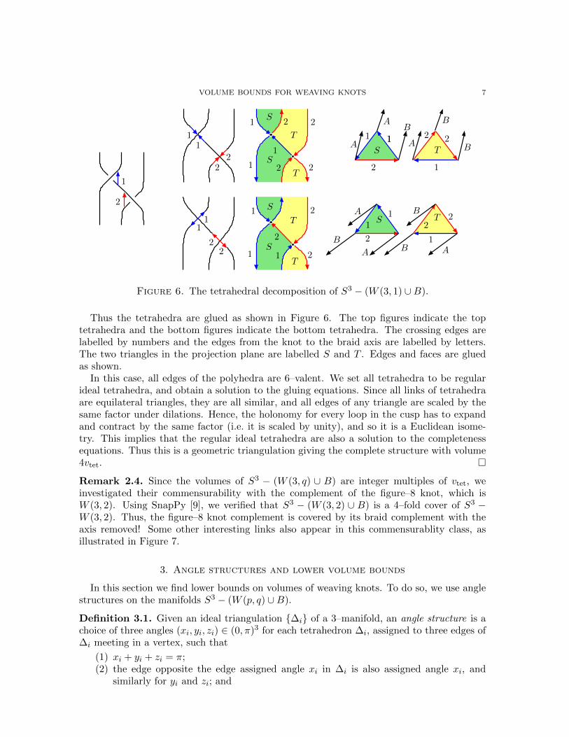
Figure 6. The tetrahedral decomposition of S3 − (W (3, 1) ∪B).

Thus the tetrahedra are glued as shown in Figure 6. The top figures indicate the toptetrahedra and the bottom figures indicate the bottom tetrahedra. The crossing edges arelabelled by numbers and the edges from the knot to the braid axis are labelled by letters.The two triangles in the projection plane are labelled S and T . Edges and faces are gluedas shown.

In this case, all edges of the polyhedra are 6–valent. We set all tetrahedra to be regularideal tetrahedra, and obtain a solution to the gluing equations. Since all links of tetrahedraare equilateral triangles, they are all similar, and all edges of any triangle are scaled by thesame factor under dilations. Hence, the holonomy for every loop in the cusp has to expandand contract by the same factor (i.e. it is scaled by unity), and so it is a Euclidean isome-try. This implies that the regular ideal tetrahedra are also a solution to the completenessequations. Thus this is a geometric triangulation giving the complete structure with volume4vtet. �

Remark 2.4. Since the volumes of S3 − (W (3, q) ∪ B) are integer multiples of vtet, weinvestigated their commensurability with the complement of the figure–8 knot, which isW (3, 2). Using SnapPy [9], we verified that S3 − (W (3, 2) ∪ B) is a 4–fold cover of S3 −W (3, 2). Thus, the figure–8 knot complement is covered by its braid complement with theaxis removed! Some other interesting links also appear in this commensurablity class, asillustrated in Figure 7.

3. Angle structures and lower volume bounds

In this section we find lower bounds on volumes of weaving knots. To do so, we use anglestructures on the manifolds S3 − (W (p, q) ∪B).

Definition 3.1. Given an ideal triangulation {∆i} of a 3–manifold, an angle structure is achoice of three angles (xi, yi, zi) ∈ (0, π)3 for each tetrahedron ∆i, assigned to three edges of∆i meeting in a vertex, such that

(1) xi + yi + zi = π;(2) the edge opposite the edge assigned angle xi in ∆i is also assigned angle xi, and

similarly for yi and zi; and


= Borromean link ∪BW (3, 3) ∪B

W (3, 2) ∪B

W (3, 2) = 41

W (3, 1) ∪B = L6a2

W (3, 6) ∪B

3

2

24

Figure 7. The complement of the figure–8 knot and its braid axis, S3 −(W (3, 2)∪B), is a 4–fold cover of the figure–8 knot complement, S3−W (3, 2).

(3) angles about any edge add to 2π.

For any tetrahedron ∆i and angle assignment (xi, yi, zi) satisfying (1) and (2) above, thereexists a unique hyperbolic ideal tetrahedron with the same dihedral angles. The volume ofthis hyperbolic ideal tetrahedron can be computed from (xi, yi, zi). We do not need the exactformula for our purposes. However, given an angle structure on a triangulation {∆i}, we cancompute the corresponding volume by summing all volumes of ideal tetrahedra with thatangle assignment.

Lemma 3.2. For p > 3, the manifold S3 − (W (p, 1) ∪ B) admits an angle structure withvolume voct (p− 2).

Proof. We will take our ideal polyhedral decomposition of S3−(W (p, 1)∪B) from Lemma 2.1and turn it into an ideal triangulation by stellating the octahedra, splitting each of theminto four ideal tetrahedra. More precisely, this is done by adding an edge running from theideal vertex on the braid axis above the plane of projection, through the plane of projectionto the ideal vertex on the braid axis below the plane of projection. Using this ideal edge,the octahedron is split into four tetrahedra.

Now obtain an angle structure on this triangulation as follows. First, assign to eachedge in an octahedron (edges that existed before stellating) the angle π/2. As for the fourtetrahedra, assign angles π/4, π/4, and π/2 to each, such that pairs of the tetrahedra glueinto squares in the cusp neighborhood of the braid axis. See Figure 3. When we stellate,assign angle structures to the four new tetrahedra coming from the octahedra in the obviousway, namely, on each new tetrahedron the ideal edge through the plane of projection is givenangle π/2, and the other two edges meeting that edge in an ideal vertex are labeled π/4.With these angles, items (1) and (2) from Definition 3.1 are satisfied for the tetrahedra. Weneed to check item (3).

Note the angle sum around each new edge in the stellated octahedra is 2π, so we onlyneed to consider edges coming from the original tetrahedra and octahedra of the polyhedral


3

12

2

2

23

3

3

1

1 1

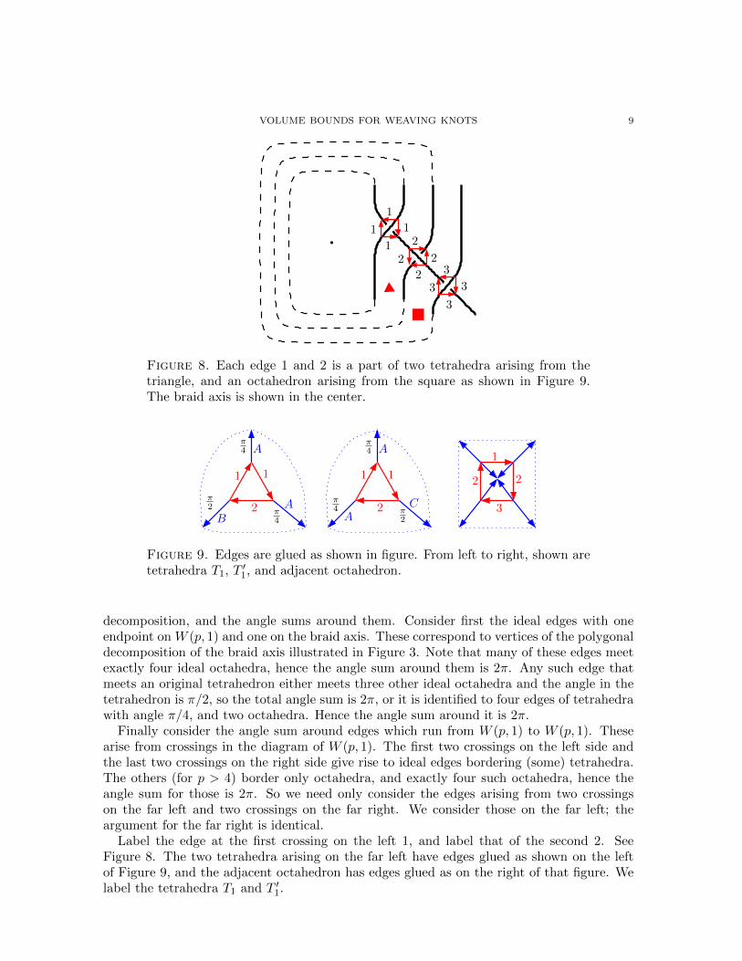
Figure 8. Each edge 1 and 2 is a part of two tetrahedra arising from thetriangle, and an octahedron arising from the square as shown in Figure 9.The braid axis is shown in the center.

π4

2

1 1

2

1 1

A

AB A

C

A1

22

3π2

π4

π2

π4

π4

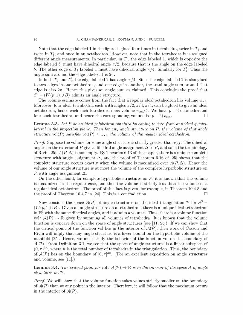
Figure 9. Edges are glued as shown in figure. From left to right, shown aretetrahedra T1, T

′1, and adjacent octahedron.

decomposition, and the angle sums around them. Consider first the ideal edges with oneendpoint on W (p, 1) and one on the braid axis. These correspond to vertices of the polygonaldecomposition of the braid axis illustrated in Figure 3. Note that many of these edges meetexactly four ideal octahedra, hence the angle sum around them is 2π. Any such edge thatmeets an original tetrahedron either meets three other ideal octahedra and the angle in thetetrahedron is π/2, so the total angle sum is 2π, or it is identified to four edges of tetrahedrawith angle π/4, and two octahedra. Hence the angle sum around it is 2π.

Finally consider the angle sum around edges which run from W (p, 1) to W (p, 1). Thesearise from crossings in the diagram of W (p, 1). The first two crossings on the left side andthe last two crossings on the right side give rise to ideal edges bordering (some) tetrahedra.The others (for p > 4) border only octahedra, and exactly four such octahedra, hence theangle sum for those is 2π. So we need only consider the edges arising from two crossingson the far left and two crossings on the far right. We consider those on the far left; theargument for the far right is identical.

Label the edge at the first crossing on the left 1, and label that of the second 2. SeeFigure 8. The two tetrahedra arising on the far left have edges glued as shown on the leftof Figure 9, and the adjacent octahedron has edges glued as on the right of that figure. Welabel the tetrahedra T1 and T ′1.


Note that the edge labeled 1 in the figure is glued four times in tetrahedra, twice in T1 andtwice in T ′1, and once in an octahedron. However, note that in the tetrahedra it is assigneddifferent angle measurements. In particular, in T1, the edge labeled 1, which is opposite theedge labeled b, must have dihedral angle π/2, because that is the angle on the edge labeledb. The other edge of T1 labeled 1 must have dihedral angle π/4. Similarly for T ′1. Thus theangle sum around the edge labeled 1 is 2π.

In both T1 and T ′1, the edge labeled 2 has angle π/4. Since the edge labeled 2 is also gluedto two edges in one octahedron, and one edge in another, the total angle sum around thatedge is also 2π. Hence this gives an angle sum as claimed. This concludes the proof thatS3 − (W (p, 1) ∪B) admits an angle structure.

The volume estimate comes from the fact that a regular ideal octahedron has volume voct.Moreover, four ideal tetrahedra, each with angles π/2, π/4, π/4, can be glued to give an idealoctahedron, hence each such tetrahedron has volume voct/4. We have p − 3 octahedra andfour such tetrahedra, and hence the corresponding volume is (p− 2) voct. �

Lemma 3.3. Let P be an ideal polyhedron obtained by coning to ±∞ from any ideal quadri-lateral in the projection plane. Then for any angle structure on P , the volume of that anglestructure vol(P ) satisfies vol(P ) ≤ voct, the volume of the regular ideal octahedron.

Proof. Suppose the volume for some angle structure is strictly greater than voct. The dihedralangles on the exterior of P give a dihedral angle assignment ∆ to P , and so in the terminologyof Rivin [25], A(P,∆) is nonempty. By Theorem 6.13 of that paper, there is a unique completestructure with angle assignment ∆, and the proof of Theorem 6.16 of [25] shows that thecomplete structure occurs exactly when the volume is maximized over A(P,∆). Hence thevolume of our angle structure is at most the volume of the complete hyperbolic structure onP with angle assignment ∆.

On the other hand, for complete hyperbolic structures on P , it is known that the volumeis maximized in the regular case, and thus the volume is strictly less than the volume of aregular ideal octahedron. The proof of this fact is given, for example, in Theorem 10.4.8 andthe proof of Theorem 10.4.7 in [24]. This is a contradiction. �

Now consider the space A(P) of angle structures on the ideal triangulation P for S3 −(W (p, 1)∪B). Given an angle structure on a tetrahedron, there is a unique ideal tetrahedronin H3 with the same dihedral angles, and it admits a volume. Thus, there is a volume functionvol : A(P) → R given by summing all volumes of tetrahedra. It is known that the volumefunction is concave down on the space of angle structures (see [11, 25]). If we can show thatthe critical point of the function vol lies in the interior of A(P), then work of Casson andRivin will imply that any angle structure is a lower bound on the hyperbolic volume of themanifold [25]. Hence, we must study the behavior of the function vol on the boundary ofA(P). From Definition 3.1, we see that the space of angle structures is a linear subspace of(0, π)3n, where n is the total number of tetrahedra in the triangulation. Thus, the boundaryof A(P) lies on the boundary of [0, π]3n. (For an excellent exposition on angle structuresand volume, see [11].)

Lemma 3.4. The critical point for vol : A(P)→ R is in the interior of the space A of anglestructures on P.

Proof. We will show that the volume function takes values strictly smaller on the boundaryof A(P) than at any point in the interior. Therefore, it will follow that the maximum occursin the interior of A(P).


Suppose we have a point X on the boundary of A(P) that maximizes volume. Because thepoint is on the boundary, there must be at least one triangle ∆ with angles (x0, y0, z0) whereone of x0, y0, and z0 equals zero or π. If one equals π, then condition (1) of Definition 3.1implies another equals zero. So we assume one of x0, y0, or z0 equals zero. A proposition ofGueritaud, [14, Proposition 7.1], implies that if one of x0, y0, z0 is zero, then another is π andthe third is also zero. (The proposition is stated for once–punctured torus bundles in [14],but only relies on the formula for volume of a single ideal tetrahedron, [14, Proposition 6.1].)

A tetrahedron with angles 0, 0, and π is a flattened tetrahedron, and contributes nothingto volume. We consider which tetrahedra might be flattened.

Let P0 be the original polyhedral decomposition described in the proof of Lemma 2.1.Suppose first that we have flattened one of the four tetrahedra which came from tetrahedrain P0. Then the maximal volume we can obtain from these four tetrahedra is at most 3 vtet,which is strictly less than voct, which is the volume we obtain from these four tetrahedrafrom the angle structure of Lemma 3.2. Thus, by Lemma 3.3, the maximal volume we canobtain from any such angle structure is 3 vtet + (p − 3)voct < (p − 2)voct. Since the volumeon the right is realized by an angle structure in the interior by Lemma 3.2, the maximum ofthe volume cannot occur at such a point of the boundary.

Now suppose one of the four tetrahedra coming from an octahedron is flattened. Then theremaining three tetrahedra can have volume at most 3 vtet < voct. Thus the volume of sucha structure can be at most 4 vtet + 3 vtet + (p− 4) voct, where the first term comes from themaximum volume of the four tetrahedra in P0, the second from the maximum volume of thestellated octahedron with one flat tetrahedron, and the last term from the maximal volumeof the remaining ideal octahedra. Because 7 vtet < 2 voct, the volume of this structure is stillstrictly less than that of Lemma 3.2.

Therefore, there does not exist X on the boundary of the space of angle structures thatmaximizes volume. �

Theorem 3.5. If p > 3, then

voct (p− 2)q ≤ vol(W (p, q) ∪B) < (voct (p− 3) + 4vtet)q.

If p = 3, then vol(W (3, q) ∪B) = 4q vtet.

Proof. Theorem 2.3 provides the p = 3 case.For p > 3, Casson and Rivin showed that if the critical point for the volume is in the

interior of the space of angle structures, then the maximal volume angle structure is realizedby the actual hyperbolic structure [25]. By Lemma 3.4, the critical point for volume is in theinterior of the space of angle structures. By Lemma 3.2, the volume of one particular anglestructure is voct (p− 2)q. So the maximal volume must be at least this. The upper bound isfrom Corollary 2.2. �

Since S3 −W (p, q) is obtained from S3 − (W (p, q) ∪B) by Dehn filling along a meridianslope, we obtain geometric information on W (p, q) given information on the geometry ofthis slope. In particular, the boundary of any embedded horoball neighborhood of the cuspB inherits a Euclidean metric, and a closed geodesic representing the meridian inherits alength in this metric, called the slope length. Note that slope length depends on choice ofhoroball neighborhood of B. Throughout, we will choose the horoball neighborhood of B tobe maximal, meaning it is tangent to itself.

Lemma 3.6. The length of a meridian of the braid axis is at least q.


Proof. A meridian of the braid axis of W (p, q) is a q–fold cover of a meridian of the braidaxis of W (p, 1). In a maximal cusp neighborhood, the meridian of the braid axis of W (p, 1)must have length at least one (see [3, 27]). Hence the meridian of the braid axis of W (p, q)has length at least q. �

We can now prove our main result on volumes of weaving knots:

Proof of Theorem 1.1. The upper bound is from Corollary 2.2.As for the lower bound, the manifold S3−W (p, q) is obtained by Dehn filling the meridian

on the braid axis of S3 − (W (p, q) ∪B). When q > 6, Lemma 3.6 implies that the meridianof the braid axis has length greater than 2π, and so [12, Theorem 1.1] will apply. Combining[12, Theorem 1.1] with Theorem 3.5 implies, for p > 3,(

1−(

2π

q

)2)3/2

((p− 2) q voct) ≤ vol(S3 −W (p, q)).

For p = 3, (1−

(2π

q

)2)3/2

(4 q vtet) ≤ vol(S3 −W (3, q)).

Since voct < 4vtet, this equation gives the desired lower bound when p = 3. Thus we havethe result for all p ≥ 3. �

Corollary 3.7. The links Kn = W (3, n) satisfy limn→∞

vol(Kn)

c(Kn)= 2vtet.

Proof. By Theorem 2.3 and the same argument as above, for q > 6 we have(1−

(2π

q

)2)3/2

(4q vtet) ≤ vol(S3 −W (3, q)) < 4q vtet. �

4. Geometric convergence of weaving knots

In this section, we will prove Theorem 1.2, which states that as p, q → ∞, the manifoldS3 −W (p, q) approaches R3 −W as a geometric limit.

A regular ideal octahedron is obtained by gluing two square pyramids, which we will callthe top and bottom pyramids. The manifold R3 −W is cut into square pyramids, which areglued into ideal octahedra, by a decomposition similar to that in Lemma 2.1. We give asketch of the decomposition here; a more detailed description is given in [8].

First, note that R3 − W admits a Z2 symmetry. The quotient of R3 − W by Z2 givesa link in the manifold T 2 × [−1, 1], with four strands forming a square on the torus T 2,with alternating crossings. As in the proof of Lemma 2.1, take an edge for each of thesefour crossings. For each of the strands, take an additional edge running from that strandto T 2 × {+1}. These crossing edges bound squares on the projection plane T 2 × {0}. Theadditional edges give boundary edges of a top pyramid. Similarly, edges running from strandson T 2 × {0} to T 2 × {−1} give edges of bottom pyramids. When we apply the Z2 action,

we obtain a division of R3 −W into X1, obtained by gluing top pyramids along triangularfaces, and X2, obtained by gluing bottom pyramids. A fundamental domain PW for R3−Win H3 is explicitly obtained by attaching each top pyramid of X1 to a bottom pyramid ofX2 along their common square face, obtaining an octahedron. In [8, Theorem 3.1], we showthat a complete hyperbolic structure on R2 −W is obtained when each octahedron is given


the structure of a regular ideal octahedron. Thus the universal cover of R3 −W is obtainedby tesselating H3 with ideal octahedra. Figure 10(a) shows how the square pyramids in X1

are viewed from infinity on the xy-plane.An appropriate π/2 rotation is needed when gluing the square faces of X1 and X2, which

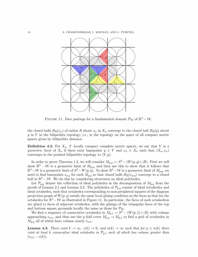
determines how adjacent triangular faces are glued to obtain PW . Figure 11 shows the facepairings for the triangular faces of the bottom square pyramids, and the associated circlepattern. The face pairings are equivariant under the translations (x, y) 7→ (x ± 1, y ± 1).That is, when a pair of faces is identified, then the corresponding pair of faces under thistranslation is also identified.

The proof below provides the geometric limit of the polyhedra described in Section 2. Wewill see that these polyhedra converge as follows. If we cut the torus in Figure 4 in halfalong the horizontal plane shown, each half is tessellated mostly by square pyramids, as wellas some tetrahedra. As p, q → ∞, the tetrahedra are pushed off to infinity, and the squarepyramids converge to the square pyramids that are shown in Figure 10. Gluing the twohalves of the torus along the square faces of the square pyramids, in the limit we obtain thetessellation by regular ideal octahedra.

(a) (b)

Figure 10. (a) Circle pattern for hyperbolic planes of the top polyhedron ofR3 −W. (b) Hyperbolic planes bounding one top square pyramid.

To make this precise, we review the definition of a geometric limit. We use bilipschitzconvergence (also called “quasi-isometry” in [5]). Convergence of metric spaces was studiedin detail by Gromov [13]. Careful treatments of geometric limits in the hyperbolic case aregiven, for example, in [7] and [5, Chapter E]. The formulation below will suffice for ourpurposes.

Definition 4.1. For compact metric spaces X and Y , define their bilipschitz distance to be

inf{| log Lip(f)|+ | log Lip(f−1)|}

where the infimum is taken over all bilipschitz mappings f from X to Y , and Lip(f) denotesthe lipschitz constant; i.e., the minimum value of K such that

1

Kd(x, y) ≤ d(f(x), f(y) ≤ K d(x, y)

for all x, y in X. The lipschitz constant is defined to be infinite if there is no bilipschitz mapbetween X and Y .

A sequence {(Xn, xn)} of locally compact complete length metric spaces with distinguishedbasepoints is said to converge in the pointed bilipschitz topology to (Y, y) if for any R > 0,


a a

d

db

c c

b

Figure 11. Face pairings for a fundamental domain PW of R3 −W.

the closed balls BR(xn) of radius R about xn in Xn converge to the closed ball BR(y) abouty in Y in the bilipschitz topology; i.e., in the topology on the space of all compact metricspaces given by bilipschitz distance.

Definition 4.2. For Xn, Y locally compact complete metric spaces, we say that Y is ageometric limit of Xn if there exist basepoints y ∈ Y and xn ∈ Xn such that (Xn, xn)converges in the pointed bilipschitz topology to (Y, y).

In order to prove Theorem 1.2, we will consider Mp,q := S3 − (W (p, q)∪B). First we willshow R3 − W is a geometric limit of Mp,q, and then use this to show that it follows thatR3−W is a geometric limit of S3−W (p, q). To show R3−W is a geometric limit of Mp,q, weneed to find basepoints xp,q for each Mp,q so that closed balls BR(xp,q) converge to a closedball in R3 −W. We do this by considering structures on ideal polyhedra.

Let Pp,q denote the collection of ideal polyhedra in the decomposition of Mp,q from theproofs of Lemma 2.1 and Lemma 3.2. The polyhedra of Pp.q consist of ideal tetrahedra andideal octahedra, such that octahedra corresponding to non-peripheral squares of the diagramprojection graph of W (p, q) satisfy the same local gluing condition on the faces as that for theoctahedra for R3−W as illustrated in Figure 11. In particular, the faces of each octahedronare glued to faces of adjacent octahedra, with the gluings of the triangular faces of the topand bottom square pyramids locally the same as those for PW .

We find a sequence of consecutive octahedra in Mp,1 = S3 − (W (p, 1) ∪ B) with volumeapproaching voct, and then use the q–fold cover Mp,q → Mp,1 to find a grid of octahedra inMp,q all of which have volume nearly voct.

Lemma 4.3. There exist k → ∞, ε(k) → 0, and n(k) → ∞ such that for p ≥ n(k) thereexist at least k consecutive ideal octahedra in Pp,1 each of which has volume greater than(voct − ε(k)).


Proof. Let ε(k) = 1k and n(k) = k3. Suppose there are no k consecutive octahedra each of

whose volume is greater than voct − ε(k). This implies that there exist at least n(k)/k = k2

octahedra each of which has volume at most voct − ε(k). Hence for k > 12 and p > n(k),

vol(Mp,1) ≤ 4vtet + (p− k2)voct + k2(voct − 1/k)

= 4vtet + pvoct − k= (p− 2)voct + 4vtet + 2voct − k< (p− 2)voct.

This contradicts Theorem 3.5, which says that (p− 2)voct < vol(Mp,1). �

Corollary 4.4. For any ε > 0 and any k > 0 there exists N such that if p, q > N thenPp,q contains a k× k grid of adjacent ideal octahedra, each of which has volume greater than(voct − ε).

Proof. Apply Lemma 4.3, taking k sufficiently large so that ε(k) < ε. Then for any N > n(k),if p > N we obtain at least k consecutive ideal octahedra with volume as desired. Now letq > N , so q > k. Use the q–fold cover Mp,q → Mp,1. We obtain a k × q grid of octahedra,all of which have volume greater than (voct − ε(k)), as shown in Figure 12. �

Figure 12. Grid of octahedra with volumes near voct in Pp,q, and base point.

We are now ready to complete the proof of Theorem 1.2.

Proof of Theorem 1.2. Given R > 0, we will show that closed balls based in Mp,q convergeto a closed ball based in R3 −W.

Take a basepoint y ∈ R3−W to lie in the interior of any octahedron, on one of the squaresprojecting to a checkerboard surface, say at the point where the diagonals of that squareintersect. Consider the ball BR(y) of radius R about the basepoint y. This will intersectsome number of regular ideal octahedra. Notice that the octahedra are glued on all faces toadjacent octahedra, by the gluing pattern we obtained in Figure 11. Consider all octahedrain R3 −W that meet the ball BR(y). Call this collection of octahedra Oct(R).

In Mp,q, consider an octahedron of Lemma 2.1 coming from a square in the interior ofthe diagram of W (p, q), so that the octahedron is glued only to other octahedra in thepolyhedral decomposition. Then the gluing pattern on each of its faces agrees with thegluing of octahedra in R3 − W. Thus for p, q large enough, we may find a collection ofadjacent octahedra Octp,q in Mp,q with the same combinatorial gluing pattern as Oct(R).Since all the octahedra are glued along faces to adjacent octahedra, Corollary 4.4 impliesthat if we choose p, q large enough, then each ideal octahedron in Octp,q has volume withinε of voct.

It is known that the volume of a hyperbolic ideal octahedron is uniquely maximized bythe volume of a regular ideal octahedron (see, e.g. [24, Theorem 10.4.7]). Thus as ε → 0,each ideal octahedron of Octp,q must be converging to a regular ideal octahedron. So Octp,q


converges as a polyhedron to Oct(R). But then it follows that for suitable basepoints xp,q inPp,q, the balls BR(xp,q) in Pp,q ⊂Mp,q converge to BR(y) in the pointed bilipschitz topology.

Finally, we use the fact that Mp,q = S3− (W (p, q)∪B) converges to R3−W geometricallyto show that S3−W (p, q) also converges to R3−W geometrically. This will follow from thedrilling/filling theorems of Hodgson and Kerckhoff [15], Brock and Bromberg [6], using theformulation of Magid [20]. Recall that S3−W (p, q) is obtained from Mp,q by Dehn filling themeridian slope of the cusp of Mp,q corresponding to the braid axis B of W (p, q). The drillingand filling theorems control geometry change under Dehn filling, provided the normalizedlength of the Dehn filling slope is sufficiently long, where normalized length is defined to bethe length of the slope divided by the square root of the area of the cusp torus containingthe slope.

By Lemma 3.6, the length of the Dehn filling slope is at least q. Moreover, because thebraid axis of W (p, q) is q-fold covered by the braid axis of W (p, 1), the area of the cuspcorresponding to B of Mp,q is q times the area of the cusp corresponding to the braid axisfor Mp,1. Thus the normalized length of the slope is at least c

√q, where c is some positive

constant. It follows that as q goes to infinity, normalized length also goes to infinity.Now apply [20, Theorem 1.2]. This theorem states that for any bilipschitz constant J > 1,

and any ε > 0, there is a universal constantK such that for any geometrically finite hyperbolic3-manifold M with no annular cusp, and with a distinguished torus cusp T (in our case,

M = Mp,q with cusp T = B), and any slope β on T with normalized length at least K, thereexists a J-bilipschitz diffeomorphism from the complement of an ε-thin neighborhood of thecusp T in M to the complement of an ε-thin neighborhood of the tube about the filled curvein the filled manifold M(β). Since we already know that compact balls in Mp,q converge tothose in R3 −W in the pointed bilipschitz topology, it follows that by choosing appropriatesequences of ε and J in the filling theorem, and letting q →∞, corresponding compact ballsin S3 −W (p, q) also converge to those in R3 −W, and thus R3 −W is a geometric limit ofS3 −W (p, q). �

References

1. Colin Adams, Triple crossing number of knots and links, J. Knot Theory Ramifications 22 (2013), no. 2,1350006, 17.

2. , Generalized augmented alternating links and hyperbolic volumes, arXiv:1506.0302 [math.GT],2015.

3. Colin C. Adams, Waist size for cusps in hyperbolic 3-manifolds, Topology 41 (2002), no. 2, 257–270.4. Ian Agol, Peter A. Storm, and William P. Thurston, Lower bounds on volumes of hyperbolic Haken

3-manifolds, J. Amer. Math. Soc. 20 (2007), no. 4, 1053–1077, With an appendix by Nathan Dunfield.5. Riccardo Benedetti and Carlo Petronio, Lectures on hyperbolic geometry, Universitext, Springer-Verlag,

Berlin, 1992.6. Jeffrey F. Brock and Kenneth W. Bromberg, On the density of geometrically finite Kleinian groups, Acta

Math. 192 (2004), no. 1, 33–93.7. R. D. Canary, D. B. A. Epstein, and P. L. Green, Notes on notes of Thurston [mr0903850], Fundamentals

of hyperbolic geometry: selected expositions, London Math. Soc. Lecture Note Ser., vol. 328, CambridgeUniv. Press, Cambridge, 2006, With a new foreword by Canary, pp. 1–115.

8. Abhijit Champanerkar, Ilya Kofman, and Jessica S. Purcell, Geometrically and diagrammatically maximalknots, arXiv:1411.7915 [math.GT], v3 (2015).

9. Marc Culler, Nathan M. Dunfield, Matthias Goerner, and Jeffrey R. Weeks, SnapPy, a computer programfor studying the geometry and topology of 3-manifolds, Available at http://snappy.computop.org.

10. Oliver Dasbach and Anastasiia Tsvietkova, A refined upper bound for the hyperbolic volume of alternatinglinks and the colored Jones polynomial, Math. Res. Lett. 22 (2015), no. 4, 1047–1060.


11. David Futer and Francois Gueritaud, From angled triangulations to hyperbolic structures, Interactionsbetween hyperbolic geometry, quantum topology and number theory, Contemp. Math., vol. 541, Amer.Math. Soc., Providence, RI, 2011, pp. 159–182.

12. David Futer, Efstratia Kalfagianni, and Jessica S. Purcell, Dehn filling, volume, and the Jones polynomial,J. Differential Geom. 78 (2008), no. 3, 429–464.

13. Misha Gromov, Metric structures for Riemannian and non-Riemannian spaces, Progress in Mathematics,vol. 152, Birkhauser Boston, Inc., Boston, MA, 1999, Based on the 1981 French original [ MR0682063(85e:53051)], With appendices by M. Katz, P. Pansu and S. Semmes, Translated from the French by SeanMichael Bates.

14. Francois Gueritaud and David Futer (appendix), On canonical triangulations of once-punctured torusbundles and two-bridge link complements, Geom. Topol. 10 (2006), 1239–1284.

15. Craig D. Hodgson and Steven P. Kerckhoff, Universal bounds for hyperbolic Dehn surgery, Ann. of Math.(2) 162 (2005), no. 1, 367–421.

16. Jim Hoste and Morwen Thistlethwaite, Knotscape 1.01, available at http://www.math.utk.edu/

∼morwen/knotscape.html.17. Jim Hoste, Morwen Thistlethwaite, and Jeff Weeks, The first 1,701,936 knots, Math. Intelligencer 20

(1998), no. 4, 33–48.18. Marc Lackenby, The volume of hyperbolic alternating link complements, Proc. London Math. Soc. (3) 88

(2004), no. 1, 204–224, With an appendix by Ian Agol and Dylan Thurston.19. Borut Levart, “Slicing a Torus” from the Wolfram Demonstrations Project,

http://demonstrations.wolfram.com/SlicingATorus.20. Aaron D. Magid, Deformation spaces of Kleinian surface groups are not locally connected, Geom. Topol.

16 (2012), no. 3, 1247–1320.21. V. O. Manturov, A combinatorial representation of links by quasitoric braids, European J. Combin. 23

(2002), no. 2, 207–212.22. W. Menasco, Closed incompressible surfaces in alternating knot and link complements, Topology 23

(1984), no. 1, 37–44.23. Skip Pennock, Turk’s-Head Knots (Braided Band Knots), A Mathematical Modeling, available at

http://www.mi.sanu.ac.rs/vismath/pennock1/index.html, 2005.24. John G. Ratcliffe, Foundations of hyperbolic manifolds, Graduate Texts in Mathematics, vol. 149,

Springer-Verlag, New York, 1994.25. Igor Rivin, Euclidean structures on simplicial surfaces and hyperbolic volume, Ann. of Math. (2) 139

(1994), no. 3, 553–580.26. Morwen B. Thistlethwaite, A spanning tree expansion of the Jones polynomial, Topology 26 (1987), no. 3,

297–309.27. William P. Thurston, The geometry and topology of three-manifolds, Princeton Univ. Math. Dept. Notes,

1979.

E-mail address: [email protected]

Department of Mathematics, College of Staten Island & The Graduate Center, City Uni-versity of New York, New York, NY


Department of Mathematics, College of Staten Island & The Graduate Center, City Uni-versity of New York, New York, NY

School of Mathematical Sciences, 9 Rainforest Walk, Monash University, Victoria 3800,Australia


introduction - monash universityusers.monash.edu/~jpurcell/papers/weaving-2016.pdf · weaving knots...

Documents