introduction cfd
TRANSCRIPT
8/8/2019 Introduction Cfd
http://slidepdf.com/reader/full/introduction-cfd 1/52
n ro uc on o ompu a ona
8/8/2019 Introduction Cfd
http://slidepdf.com/reader/full/introduction-cfd 2/52
lin
1. What, why and where of CFD?
. o e ng
3. Numerical methods
5. CFD Educational Interface
6. CFD Process7. Example of CFD Process
8. 58:160 CFD Labs
2

8/8/2019 Introduction Cfd
http://slidepdf.com/reader/full/introduction-cfd 3/52
Wh i FD?
• CFD is the simulation of fluids engineering systems usingmodeling (mathematical physical problem formulation) andnumer ca me o s scre za on me o s, so vers, numer ca
parameters, and grid generations, etc.)
• Historically only Analytical Fluid Dynamics (AFD) andxper men a u ynam cs .
• CFD made possible by the advent of digital computer and
advancing with improvements of computer resources(500 flops, 194720 teraflops, 2003)
3
8/8/2019 Introduction Cfd
http://slidepdf.com/reader/full/introduction-cfd 4/52
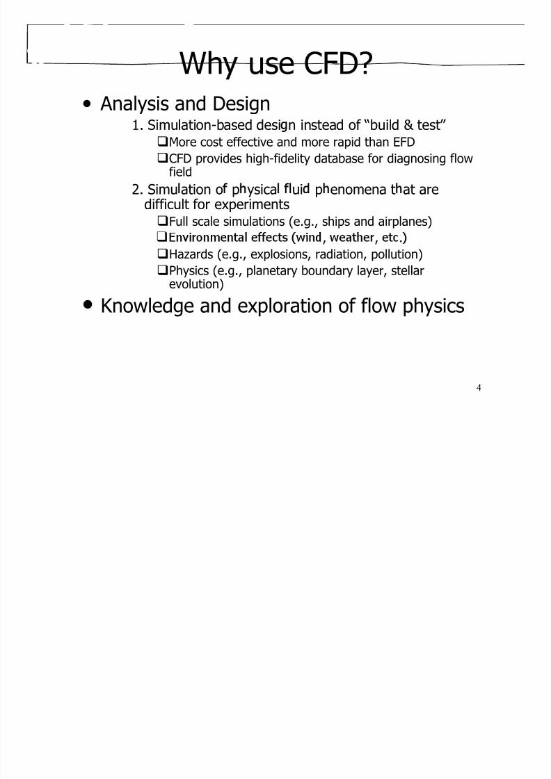
Wh use CFD?• Analysis and Design
1. Simulation-based desi n instead of “build & test”
More cost effective and more rapid than EFDCFD provides high-fidelity database for diagnosing flowfield
2. Simu ation o p ysica ui p enomena t at aredifficult for experiments
Full scale simulations (e.g., ships and airplanes), , .
Hazards (e.g., explosions, radiation, pollution)
Physics (e.g., planetary boundary layer, stellarevolution)
• Knowledge and exploration of flow physics
4
8/8/2019 Introduction Cfd
http://slidepdf.com/reader/full/introduction-cfd 5/52
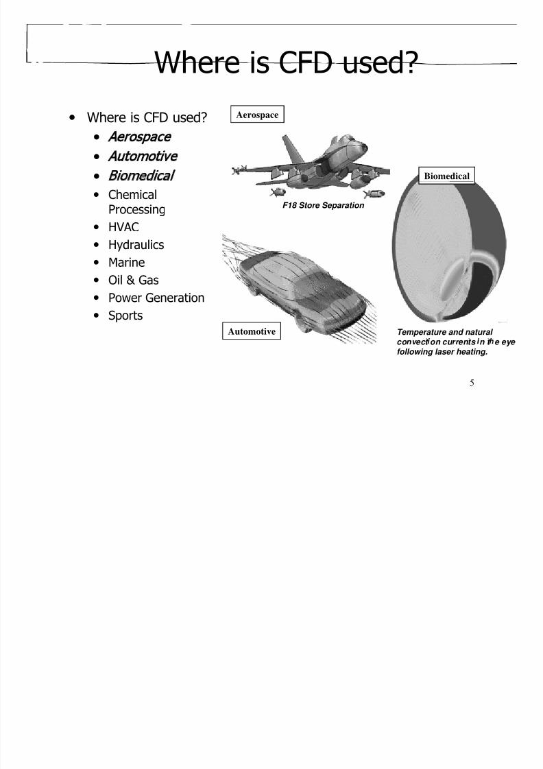
Where is CFD used?• Where is CFD used? Aerospace
• Aerospace
• Automotive
• Biomedical Biomedical
• ChemicalProcessing
• HVAC
F18 Store Separation
• Hydraulics
• Marine
• Oil & Gas
• Power Generation
• Sports
Temperature and natural Automotive
5
convect on currents n t e eye following laser heating.
8/8/2019 Introduction Cfd
http://slidepdf.com/reader/full/introduction-cfd 6/52
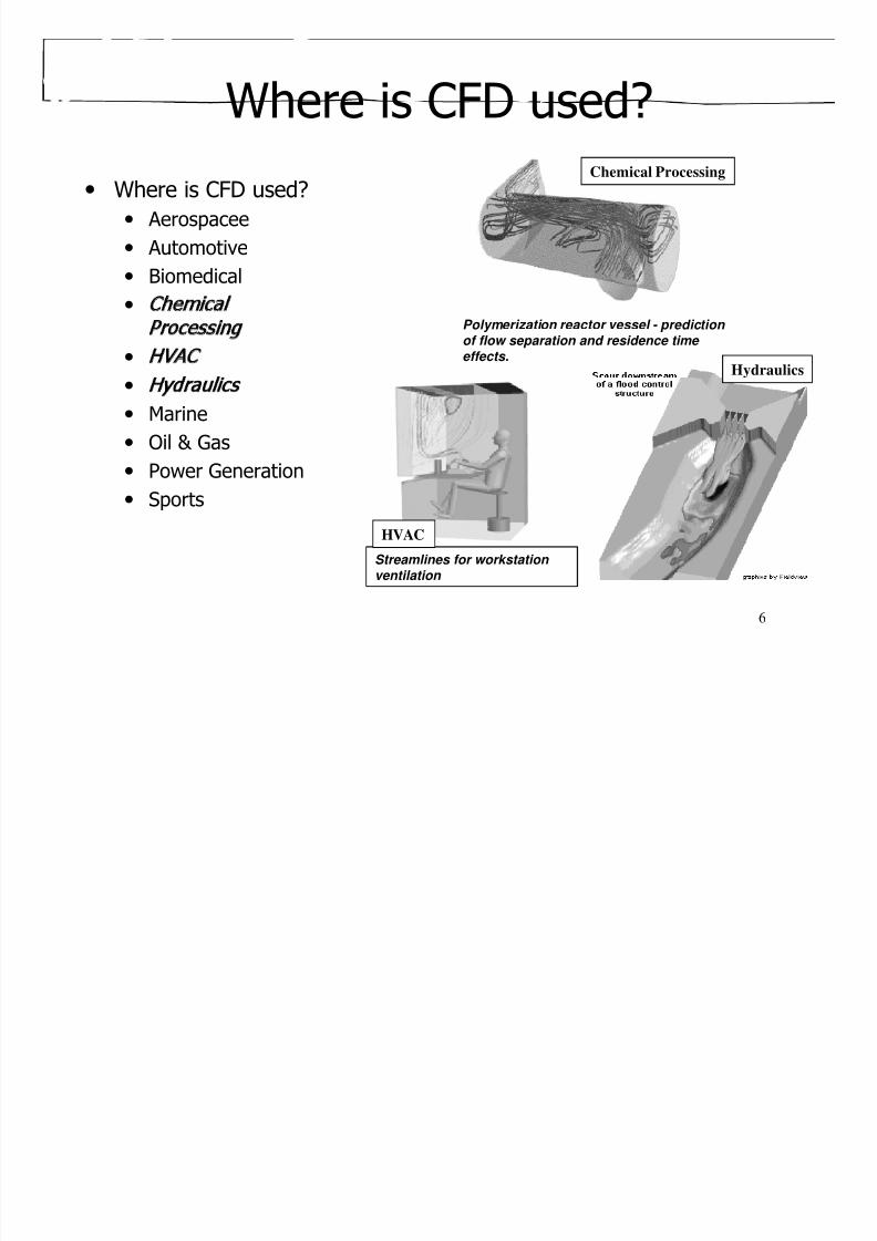
Where is CFD used?• Where is CFD used?
Chemical Processing
• Aerospacee
• Automotive
• Biomedical
Polymerization reactor vessel - prediction of flow separation and residence time
effects.
• Chemical
Processing
• HVAC
H d liHydraulics
• Hydraulics
• Marine
• Oil & Gas
• Power Generation• Sports
HVAC
6
Streamlines for workstation ventilation

8/8/2019 Introduction Cfd
http://slidepdf.com/reader/full/introduction-cfd 7/52
Where is CFD used?• Where is CFD used?
Marine (movie) Sports
• Aerospace
• Automotive
• Biomedical
• Chemical Processing
• HVAC
• Hydraulics
• Marine
• Oil & Gas
• Power Generation
• Sports
7
Flow of lubricating mud over drill bit Flow around cooling
towers
8/8/2019 Introduction Cfd
http://slidepdf.com/reader/full/introduction-cfd 8/52
Modeling• Modeling is the mathematical physics problemformulation in terms of a continuous initial
• IBVP is in the form of Partial DifferentialEquations (PDEs) with appropriate boundaryconditions and initial conditions.
• Modeling includes:
1. Geometry and domain.3. Governing equations4. Flow conditions
5. Initial and boundary conditions6. Selection of models for different applications
8

8/8/2019 Introduction Cfd
http://slidepdf.com/reader/full/introduction-cfd 9/52
Modelin eometr and domain• Simple geometries can be easily created by few geometricparameters (e.g. circular pipe)
• Com lex eometries must be created b the artialdifferential equations or importing the database of thegeometry(e.g. airfoil) into commercial software
• Domain: size and shape
• Typical approaches
• Geometry approximation• CAD/CAE integration: use of industry standards such as
Parasolid, ACIS, STEP, or IGES, etc.
• The three coordinates: Cartesian system (x,y,z), cylindrical, , , , ,
appropriately chosen for a better resolution of the geometry(e.g. cylindrical for circular pipe).
9

8/8/2019 Introduction Cfd
http://slidepdf.com/reader/full/introduction-cfd 10/52
Modeling (coordinates)z z z
(r,θ,z) (r,θ,φ)(x,y,z)
Cartesian Cylindrical Spherical
z
x x xr θ r
10
Coordinates

8/8/2019 Introduction Cfd
http://slidepdf.com/reader/full/introduction-cfd 11/52
Modeling (governing equations)• av er- o es equa ons n ar es an coor na es
⎥⎦
⎤⎢⎣
⎡
∂
∂+
∂
∂+
∂
∂+
∂
∂−=
∂
∂+
∂
∂+
∂
∂+
∂
∂2
2
2
2
2
2ˆ
z
u
y
u
x
u
x
p
z
uw
y
uv
x
uu
t
u μ ρ ρ ρ ρ
⎥⎦
⎤⎢⎣
⎡
∂∂+∂∂+∂∂+∂∂−=∂∂+∂∂+∂∂+∂∂ 2
2
2
2
2
2
ˆ z
v y
v x
v y p
zvw
yvv
xvu
t v μ ρ ρ ρ ρ
ˆ⎥⎦
⎢⎣ ∂
+∂
+∂
+∂
−=∂
+∂
+∂
+∂ 222
z
w
y
w
x
w
z
p
z
ww
y
wv
x
wu
t
w μ ρ ρ ρ ρ
( ) ( ) ( )0=
∂+
∂+
∂+
∂ wvu ρ ρ ρ ρ
Convection Piezometric pressure gradient Viscous termsLocal
acceleration
∂∂∂∂ z y xt
RT p ρ =
2
Equation of state
11
L
v p p
Dt Dt R
ρ
−=+ 2
2)(
2Rayleigh Equation
8/8/2019 Introduction Cfd
http://slidepdf.com/reader/full/introduction-cfd 12/52
Modeling (flow conditions)• Based on the physics of the fluids phenomena, CFDcan be distinguished into different categories using
• Viscous vs. inviscid (Re)
• External flow or internal flow wall bounded or not
• Turbulent vs. laminar (Re)
• Incompressible vs. compressible (Ma)• Single- vs. multi-phase (Ca)
• Thermal/density effects (Pr, γ , Gr, Ec)
• Free-surface flow Fr and surface tension We
• Chemical reactions and combustion (Pe, Da)
• etc…
12
8/8/2019 Introduction Cfd
http://slidepdf.com/reader/full/introduction-cfd 13/52
Modeling (initial conditions)
• Initial conditions (ICS, steady/unsteady flows)
• ICs should not affect final results and onl
affect convergence path, i.e. number of iterations (steady) or time steps (unsteady).
• More reasonable guess can speed up the
convergence• For complicated unsteady flow problems,
CFD codes are usually run in the steady
initial conditions
13
8/8/2019 Introduction Cfd
http://slidepdf.com/reader/full/introduction-cfd 14/52
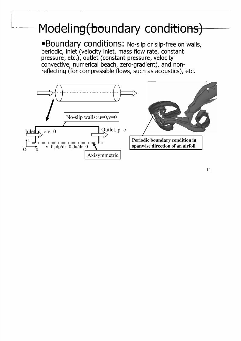
Modelin boundar conditions•Boundary conditions: No-slip or slip-free on walls,periodic, inlet (velocity inlet, mass flow rate, constant
, . , ,
convective, numerical beach, zero-gradient), and non-reflecting (for compressible flows, such as acoustics), etc.
No-slip walls: u=0,v=0
v=0, dp/dr=0,du/dr=0
Inlet ,u=c,v=0 Outlet, p=c
Periodic boundary condition in
spanwise direction of an airfoil
r
14
Axisymmetric

8/8/2019 Introduction Cfd
http://slidepdf.com/reader/full/introduction-cfd 15/52
Modeling (selection of models)• CFD codes typically designed for solving certain fluid
phenomenon by applying different models
scous vs. nv sc e
• Turbulent vs. laminar (Re, Turbulent models)
• Incom ressible vs. com ressible Ma e uation of state
• Single- vs. multi-phase (Ca, cavitation model, two-fluid
model)• erma ensity e ects an energy equation
(Pr, γ , Gr, Ec, conservation of energy)
• Free-surface flow Fr level-set & surface trackin model and
surface tension (We, bubble dynamic model)
• Chemical reactions and combustion (Chemical reaction
15
model)
• etc…

8/8/2019 Introduction Cfd
http://slidepdf.com/reader/full/introduction-cfd 16/52
Modeling (Turbulence and free surface models)
Turbulent models
• Turbulent flows at high Re usually involve both large and small scale
vortical structures and very thin turbulent boundary layer (BL) near the wall
Turbulent models
• DNS: most accurately solve NS equations, but too expensivefor turbulent flows
• RANS: predict mean flow structures, efficient inside BL but excessive
diffusion in the separated region.
• LES: accurate in separation region and unaffordable for resolving BL
• DES: RANS inside BL, LES in separated regions.
• Free-surface models:
• -
limited to small and medium wave slopes
• Single/two phase level-set method: mesh fixed and level-set
16
,
studying steep or breaking waves.

8/8/2019 Introduction Cfd
http://slidepdf.com/reader/full/introduction-cfd 17/52
Examples of modeling (Turbulence and free
surface modelsURANS, Re=105, contour of vorticity for turbulent
flow around NACA12 with angle of attack 60 degrees
DES, Re=105, Iso-surface of Q criterion (0.4) for
turbulent flow around NACA12 with angle of attack 60
degrees
17
URANS, Wigley Hull pitching and heaving

8/8/2019 Introduction Cfd
http://slidepdf.com/reader/full/introduction-cfd 18/52
Numerical methods• The continuous Initial Boundary Value Problems
using numerical methods. Assemble the system of algebraic equations and solve the system to get
• Numerical methods include:
1. Discretization methods. o vers an numer ca parame ers
3. Grid generation and transformation
4. High Performance Computation (HPC) and post-
processing
18

8/8/2019 Introduction Cfd
http://slidepdf.com/reader/full/introduction-cfd 19/52
Discretization methods• Finite difference methods (straightforward to apply,
usually for regular grid) and finite volumes and finitee emen me o s usua y or rregu ar mes es
• Each type of methods above yields the same solution if the grid is fine enough. However, some methods aremore suitable to some cases than others
• Finite difference methods for spatial derivatives withdifferent order of accuracies can be derived using
Taylor expansions, such as 2nd
order upwind scheme,central differences schemes etc. • Higher order numerical methods usually predict higher
order of accuracy for CFD, but more likely unstable dueto less numerical dissipation
explicit method (Euler, Runge-Kutta, etc.) or implicitmethod (e.g. Beam-Warming method)
19
8/8/2019 Introduction Cfd
http://slidepdf.com/reader/full/introduction-cfd 20/52
Discretization methods Cont’d• Explicit methods can be easily applied but yield
conditionally stable Finite Different Equations (FDEs),w c are res r c e y e me s ep; mp c me o s
are unconditionally stable, but need efforts onefficiency.• Usually, higher-order temporal discretization is used
when the spatial discretization is also of higher order.• Stability: A discretization method is said to be stable if
it does not magnify the errors that appear in the courseof numerical solution rocess. • Pre-conditioning method is used when the matrix of the
linear algebraic system is ill-posed, such as multi-phaseflows, flows with a broad range of Mach numbers, etc.
efficiency, accuracy and special requirements, such asshock wave tracking.
20

8/8/2019 Introduction Cfd
http://slidepdf.com/reader/full/introduction-cfd 21/52
Discretization methods (example)• 2D incompressible laminar flow boundary layer
(L,m+1)
0=∂∂+
∂∂
yv
xu
=
y
m=MMm=MM+1(L,m)(L-1,m)
2 y
u
e
p
x y
uv
x
uu
∂+⎟
⎠⎜⎝ ∂
−=∂
+∂
μ m=0
L-1 Lx
(L,m-1)
l1l lm
m m
uuu u u
x x
−⎡ ⎤= −⎣ ⎦∂ Δ2
1 12 22l l l
m m m
uu u u
y y
μ μ + −
∂⎡ ⎤= − +⎣ ⎦∂ Δ
1l lmm m
vuv u u y y
+∂ ⎡ ⎤= −⎣ ⎦∂ Δl
l lv
FD Sign( )<0l
mv 2nd order central difference
i.e., theoretical order of accuracy
P = 2.
21
1m mu u y
−= −Δ
l
mvBD Sign( )>0es
1st order upwind scheme, i.e., theoretical order of accuracy Pkest= 1
8/8/2019 Introduction Cfd
http://slidepdf.com/reader/full/introduction-cfd 22/52
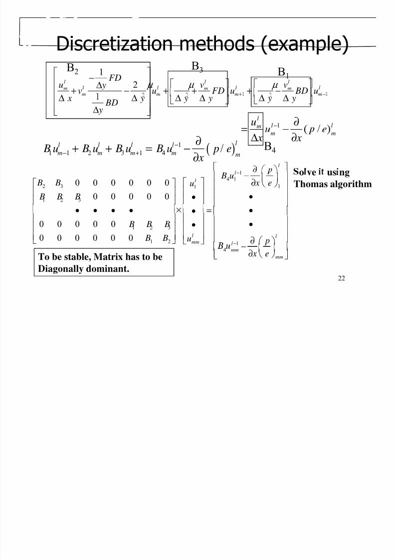
Discretization methods (example)
1
2l l ll l l lm m m
FDu v v y
v u FD u BD u μ μ μ
⎡ ⎤−⎢ ⎥ ⎡ ⎤ ⎡ ⎤Δ
+ − + + + −⎢ ⎥
B2B3 B1
x y y y y y BD
y
−Δ Δ Δ Δ Δ Δ⎢ ⎥ ⎣ ⎦ ⎣ ⎦
⎢ ⎥Δ⎣ ⎦1 /
ll lmu
u e− ∂= −m m
x xΔ ∂B4( )1
1 1 2 3 1 4 /ll l l l
m m m m m B u B u B u B u p e
x
−− +
∂+ + = −
∂ l
1
4 1
12 3 1
1 2 3
0 0 0 0 0 0
0 0 0 0 0
l
lB u
B B x eu
B B B
− −⎢ ⎥⎜ ⎟∂⎡ ⎤⎡ ⎤ ⎝ ⎠⎢ ⎥
⎢ ⎥⎢ ⎥ ⎢ ⎥••⎢ ⎥⎢ ⎥ ⎢ ⎥
o ve us ng
Thomas algorithm
1 2 3
1 2 1
0 0 0 0 0
0 0 0 0 0 0 l lmm l
B B B
B B u p−
=• • • • ••⎢ ⎥⎢ ⎥ ⎢ ⎥••⎢ ⎥⎢ ⎥ ⎢ ⎥
⎢ ⎥⎢ ⎥ ⎢ ⎥⎣ ⎦ ∂⎣ ⎦ ⎛ ⎞−
22
4 mm
mm x e−
∂⎢ ⎥⎝ ⎠⎣ ⎦To be stable, Matrix has to be
Diagonally dominant.

8/8/2019 Introduction Cfd
http://slidepdf.com/reader/full/introduction-cfd 23/52
Solvers and numerical arameters• Solvers include: tridiagonal, pentadiagonal solvers,PETSC solver, solution-adaptive solver, multi-grid
, .
• Solvers can be either direct (Cramer’s rule, Gausselimination, LU decomposition) or iterative (Jacobi
-, ,
• Numerical parameters need to be specified to control
the calculation. , , .
• Different numerical schemes
• Monitor residuals (change of results between
terat ons• Number of iterations for steady flow or number of
time steps for unsteady flow
23
• Single/double precisions
8/8/2019 Introduction Cfd
http://slidepdf.com/reader/full/introduction-cfd 24/52
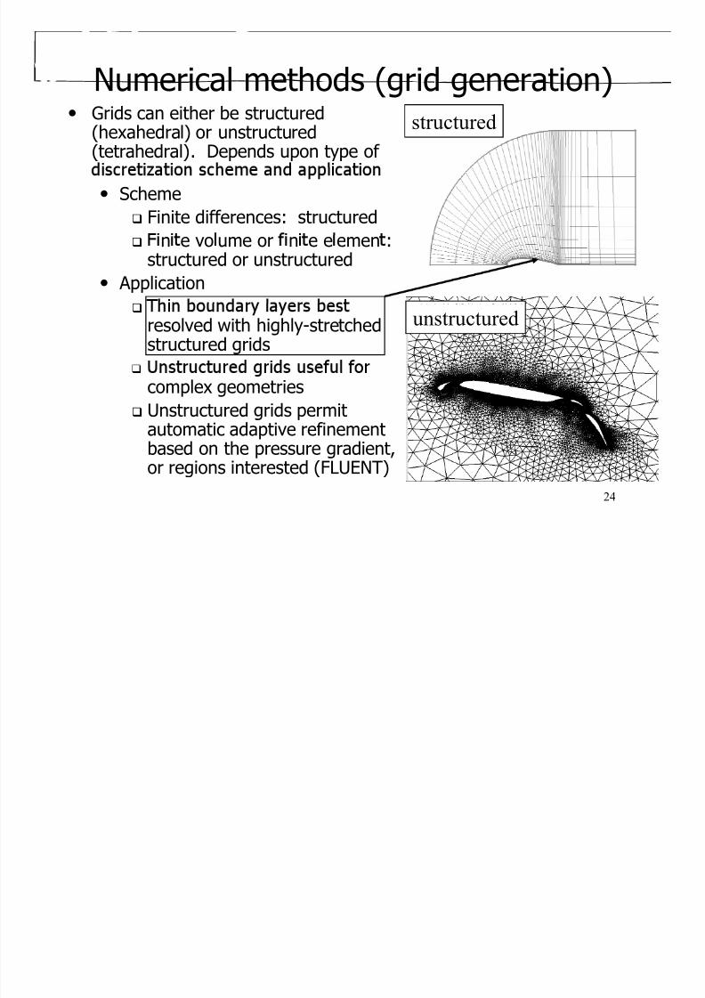
Numerical methods (grid generation)• Grids can either be structured
(hexahedral) or unstructured(tetrahedral). Depends upon type of
structured
• Scheme Finite differences: structured
n e vo ume or n e e emen :structured or unstructured
• Application
resolved with highly-stretchedstructured grids
unstructured
complex geometries Unstructured grids permit
automatic adaptive refinement
24
based on the pressure gradient,or regions interested (FLUENT)

8/8/2019 Introduction Cfd
http://slidepdf.com/reader/full/introduction-cfd 25/52
Numerical methods (grid
y η
Transform
x
o o ξ
x x
f f f f f ξ η ξ η
∂ ∂ ∂ ∂ ∂ ∂ ∂= + = +
•Transformation between physical (x,y,z)
x x xη η
y y
f f f f f
y y y
ξ η ξ η
ξ η ξ η
∂ ∂ ∂ ∂ ∂ ∂ ∂= + = +
∂ ∂ ∂ ∂ ∂ ∂ ∂
, , ,
important for body-fitted grids. The partialderivatives at these two domains have the
relationshi 2D as an exam le
25
8/8/2019 Introduction Cfd
http://slidepdf.com/reader/full/introduction-cfd 26/52
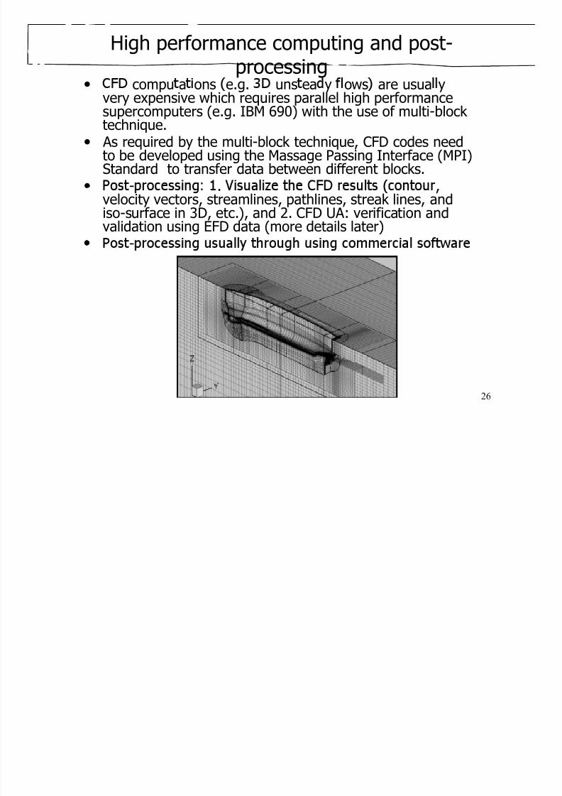
High performance computing and post-processing
• compu a ons e.g. uns ea y ows are usua yvery expensive which requires parallel high performancesupercomputers (e.g. IBM 690) with the use of multi-block technique.
• As required by the multi-block technique, CFD codes need
to be developed using the Massage Passing Interface (MPI)Standard to transfer data between different blocks.
• - . ,velocity vectors, streamlines, pathlines, streak lines, andiso-surface in 3D, etc.), and 2. CFD UA: verification and
validation using EFD data (more details later)-
26

8/8/2019 Introduction Cfd
http://slidepdf.com/reader/full/introduction-cfd 27/52
es of CFD codes• Commercial CFD code: FLUENT, Star-CD, CFDRC, CFX/AEA, etc.
• -
• Public domain software (PHI3D,HYDRO, and WinpipeD, etc.)
• Other CFD software includes the Grid generation software (e.g. Gridgen,Gambit) and flow visualization software
(e.g. Tecplot, FieldView)
27
CFDSHIPIOWA
8/8/2019 Introduction Cfd
http://slidepdf.com/reader/full/introduction-cfd 28/52
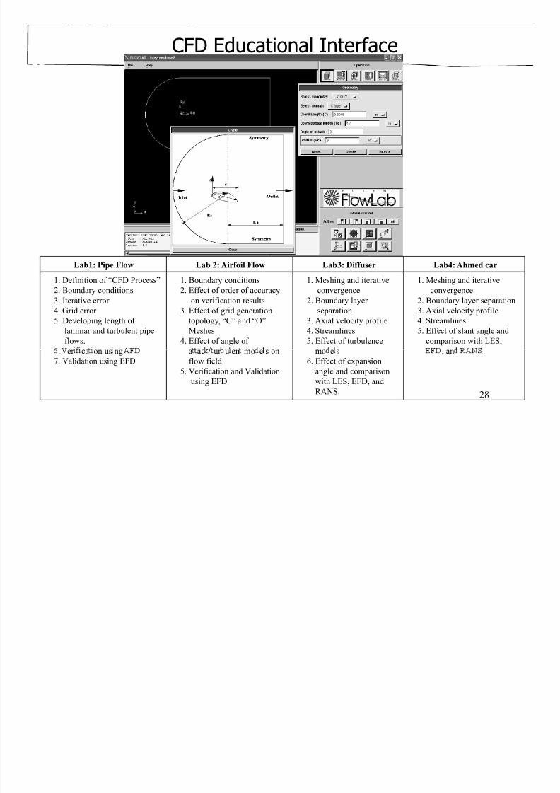
CFD Educational Interface
Lab1: Pipe Flow Lab 2: Airfoil Flow Lab3: Diffuser Lab4: Ahmed car
1. Definition of “CFD Process”
2. Boundary conditions
1. Boundary conditions
2. Effect of order of accuracy
1. Meshing and iterative
convergence
1. Meshing and iterative
convergence
3. Iterative error
4. Grid error
5. Developing length of
laminar and turbulent pipe
flows.
on verification results
3. Effect of grid generation
topology, “C” and “O”
Meshes
4. Effect of angle of
2. Boundary layer
separation
3. Axial velocity profile
4. Streamlines
5. Effect of turbulence
2. Boundary layer separation
3. Axial velocity profile
4. Streamlines
5. Effect of slant angle and
comparison with LES,
28
. er ca on us ng
7. Validation using EFD
a ac ur u en mo e s on
flow field
5. Verification and Validation
using EFD
mo e s
6. Effect of expansion
angle and comparison
with LES, EFD, andRANS.
, an .

8/8/2019 Introduction Cfd
http://slidepdf.com/reader/full/introduction-cfd 29/52
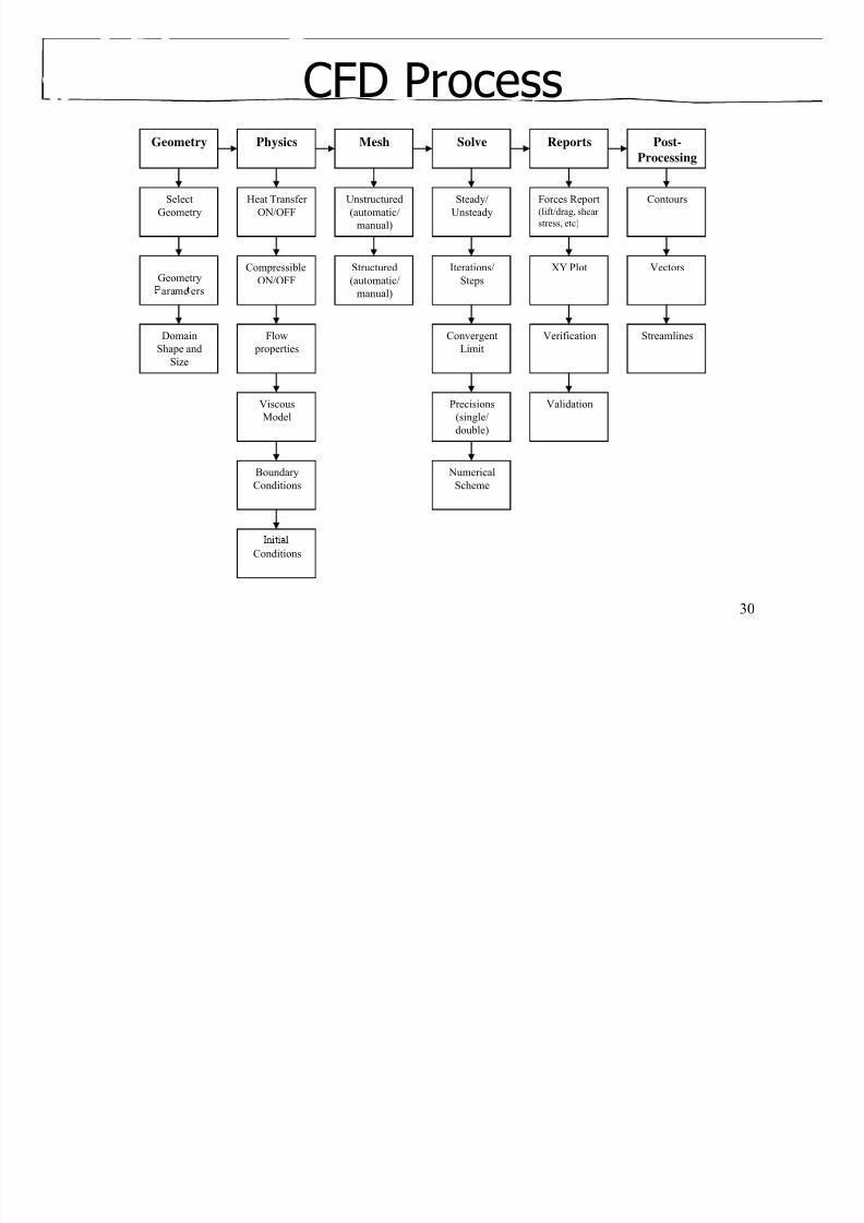
CFD rocess• Purposes of CFD codes will be different for differentapplications: investigation of bubble-fluid interactions for bubblyflows stud of wave induced massivel se arated flows for free-surface, etc.
• Depend on the specific purpose and flow conditions of theproblem, different CFD codes can be chosen for differentapp ications aerospace, marines, com ustion, mu ti-p aseflows, etc.)
• Once purposes and CFD codes chosen, “CFD process” is the
1. Geometry
2. Physics
3. Mesh4. Solve
5. Reports
29
6. Post processing
8/8/2019 Introduction Cfd
http://slidepdf.com/reader/full/introduction-cfd 30/52
CFD Process
Contours
Geometry
Select
Physics Mesh Solve Post-
Processing
Unstructured Steady/ Forces ReportHeat Transfer
Reports
Vectors
Geometry
GeometryCompressible
ON/OFF
(automatic/
manual)
Unsteady (lift/drag, shear
stress, etc)
XY Plot
ON/OFF
Structured
(automatic/
Iterations/
Steps
Convergent
Limit
StreamlinesVerification
arame ers
Flow
properties
Domain
Shape and
Size
manual)
Viscous
Model
Precisions
(single/
double)
Validation
BoundaryConditions
NumericalScheme
30
Conditions

8/8/2019 Introduction Cfd
http://slidepdf.com/reader/full/introduction-cfd 31/52
Geometr• Selection of an appropriate coordinate
• Determine the domain size and sha e
• Any simplifications needed?• What kinds of shapes needed to be used to best
resolve the geometry? (lines, circular, ovals, etc.)
• For commercial code, geometry is usually created
commercial code itself, like Gambit, or combinedtogether, like FlowLab)
• For research code, commercial software (e.g.Gridgen) is used.
31
8/8/2019 Introduction Cfd
http://slidepdf.com/reader/full/introduction-cfd 32/52
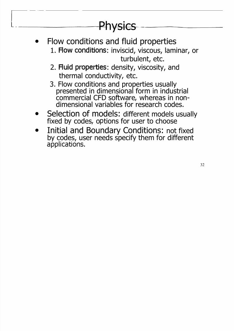
Physics• Flow conditions and fluid properties
1. Flow conditions: inviscid, viscous, laminar, orturbulent, etc.
2. Fluid properties: density, viscosity, andthermal conductivit etc.
3. Flow conditions and properties usuallypresented in dimensional form in industrial
commercial CFD software whereas in non-dimensional variables for research codes.
• Selection of models: different models usuallyfixed b codes o tions for user to choose
• Initial and Boundary Conditions: not fixedby codes, user needs specify them for different
32

8/8/2019 Introduction Cfd
http://slidepdf.com/reader/full/introduction-cfd 33/52
Mesh• Meshes should be well designed to resolveim ortant flow features which are de endent u onflow condition parameters (e.g., Re), such as thegrid refinement inside the wall boundary layer
• es can e genera e y e er commerc a co es(Gridgen, Gambit, etc.) or research code (using
algebraic vs. PDE based, conformal mapping, etc.)• The mesh, together with the boundary conditions
need to be exported from commercial software in a
research CFD code or other commercial CFDsoftware.
33

8/8/2019 Introduction Cfd
http://slidepdf.com/reader/full/introduction-cfd 34/52
Solve
• Setup appropriate numerical parameters
• oose appropr a e o vers
• Solution procedure (e.g. incompressible flows)
,equations and get flow field quantities, such as
velocit , turbulence intensit , ressure andintegral quantities (lift, drag forces)
34

8/8/2019 Introduction Cfd
http://slidepdf.com/reader/full/introduction-cfd 35/52
Re orts• Reports saved the time history of the residualsof the velocity, pressure and temperature, etc.
• Report the integral quantities, such as totalpressure drop, friction factor (pipe flow), liftand dra coefficients airfoil flow etc.
• XY plots could present the centerlinevelocity/pressure distribution, friction factor
,distribution (airfoil flow).
• AFD or EFD data can be imported and put on
35
8/8/2019 Introduction Cfd
http://slidepdf.com/reader/full/introduction-cfd 36/52
Post-processing
• Analysis and visualization• Calculation of derived variables
Vorticity
Wall shear stress• Calculation of integral parameters: forces,
moments
• Visualization (usually with commercial
software) mp e con ours
3D contour isosurface plots
Vector plots and streamlines
tangent direction is the same as thevelocity vectors)
36

8/8/2019 Introduction Cfd
http://slidepdf.com/reader/full/introduction-cfd 37/52
Post-processing (Uncertainty Assessment)
• imu ation error: the difference between a simulation resultS and the truth T (objective reality), assumed composed of additive modeling δSM and numerical δSN errors:
• Verification: process for assessing simulation numerical
SN SM S T S δ δ δ +=−=
222
SN SM S
U U U +=
uncer a n es SN an , w en con ons perm , es ma ng esign and magnitude Delta δ*
SN of the simulation numerical erroritself and the uncertainties in that error estimate UScN
J
• Validation: process for assessing simulation modelinguncertainty U SM by using benchmark experimental data and,
=
== j
j I PT G I SN
1PT G I SN U U U U U +++=
when conditions permit, estimating the sign and magnitude of the modeling error δ SM itself.
)( SN SM DS D E δ δ δ +−=−=222
SN DV U U U +=
37
V U E < Validation achieved

8/8/2019 Introduction Cfd
http://slidepdf.com/reader/full/introduction-cfd 38/52
Post-processing (UA, Verification)
• onvergence s u es: onvergence s u es requ re aminimum of m=3 solutions to evaluate convergence withrespective to input parameters. Consider the solutions
∧ ∧∧
, ,1k 2k
3k
21 2 1k k k S Sε ∧ ∧
= − 32 3 2k k k S Sε ∧ ∧
= −
(i). Monotonic convergence: 0<R k <1
ii . Oscillator Conver ence: R <0 R <1
21 32k k k R ε ε =
(iii). Monotonic divergence: R k >1
(iv). Oscillatory divergence: R k <0; | R k |>1
• .
12312 −ΔΔ=ΔΔ=ΔΔ=
mm k k k k k k k x x x x x xr
38
8/8/2019 Introduction Cfd
http://slidepdf.com/reader/full/introduction-cfd 39/52
Post-processing (Verification: Iterative
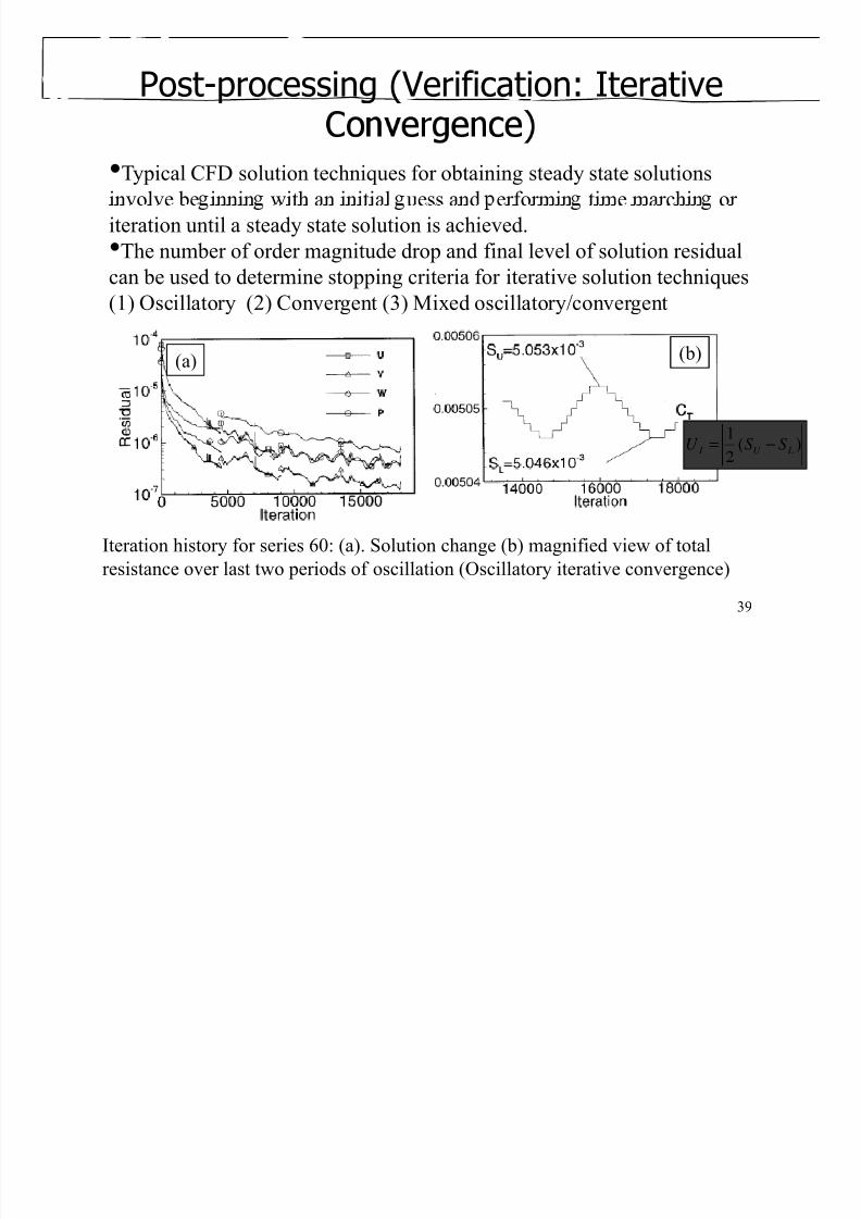
•Typical CFD solution techniques for obtaining steady state solutions
involve be innin with an initial uess and erformin time marchin or
iteration until a steady state solution is achieved.
•The number of order magnitude drop and final level of solution residual
can be used to determine stopping criteria for iterative solution techniques
(1) Oscillatory (2) Convergent (3) Mixed oscillatory/convergent
(b)(a)
)(1
LU I SSU −=
39
Iteration history for series 60: (a). Solution change (b) magnified view of total
resistance over last two periods of oscillation (Oscillatory iterative convergence)
8/8/2019 Introduction Cfd
http://slidepdf.com/reader/full/introduction-cfd 40/52
Post- rocessin Verification RE
• Generalized Richardson Extrapolation (RE): Formonotonic convergence, generalized RE is used toestimate the error δ*
k and order of accuracy p k due
to the selection of the kth input parameter.
with integer powers of Δxk as a finite sum.
• The accuracy of the estimates depends on howmany terms are retained in the expansion, themagnitude (importance) of the higher-order terms,
theory
40
Post processing (Verification RE)
8/8/2019 Introduction Cfd
http://slidepdf.com/reader/full/introduction-cfd 41/52
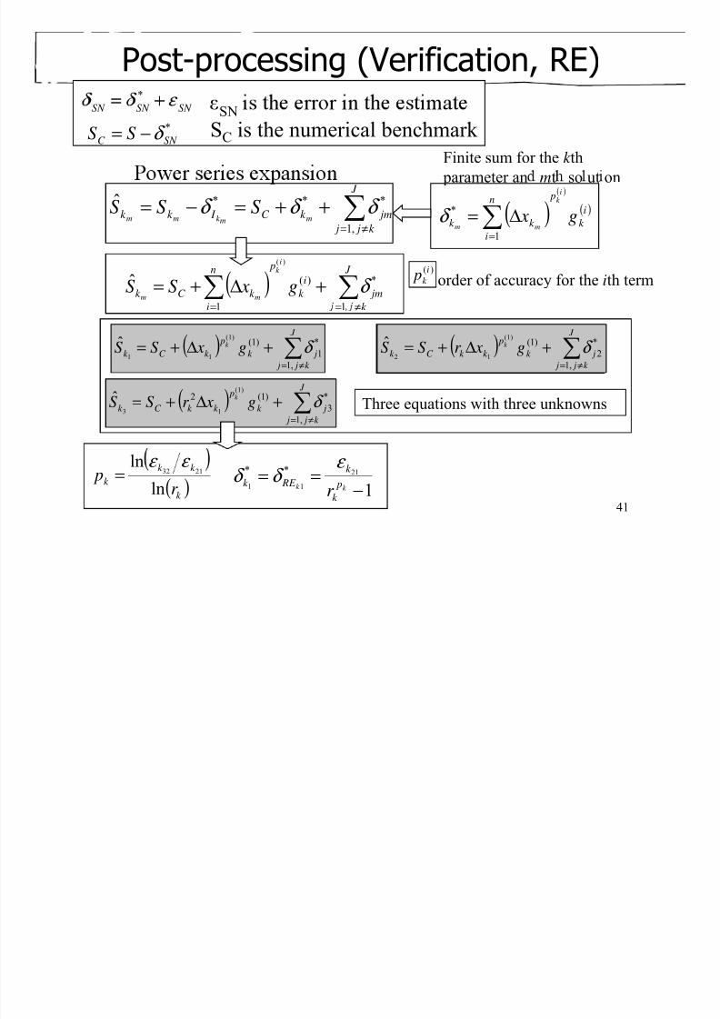
Post-processing (Verification, RE)*
Finite sum for the k th
SN SN SN
*
SN C SS δ −=SN
SC is the numerical benchmark
( )( )
( )i
k
pn
i
k k g x
i
k
mm ∑=
Δ=1
*δ ∑≠=++=−=
J
k j j
jmk C I k k mmk mmSSS
,1
***ˆ δ δ δ
parameter an mt so ut on
)(i
k p( ) ∑∑≠==
+Δ+= J
k
jm
i
k
pn
i
k C k g xSS
ik
mm 1
*)(
1
)(
ˆ δ order of accuracy for the ith term
( ) ∑≠=
+Δ+= J
k j j
jk
p
k C k g xSS k
,1
*
1
)1()1(
11
ˆ δ ( ) ∑≠=
+Δ+= J
k j j
jk
p
k k C k g xr SS k
,1
*
2
)1()1(
12
ˆ δ
Three equations with three unknowns( ) ∑≠=
+Δ+= J
k j j
jk p
k k C k g xr SS k
,1
*3
)1(2
)1(
13ˆ δ
411
21
11
**
−
==k k p
k
k
RE k
r
ε δ δ
( )k
k k
k
r
p
ln
ln2132
ε ε =

8/8/2019 Introduction Cfd
http://slidepdf.com/reader/full/introduction-cfd 42/52
Post-processing (UA, Verification, cont’d)
• Monotonic Convergence: Generalized RichardsonExtrapolation
p
1. Correction
( )
( )
32 21ln
ln
k k
k
k
p
r
ε ε =
1
k est
k k p
k
C
r
−=
−
( )1
1
*
*
9.6 1 1.1
2 1 1
k
k
k RE
k
k RE
C
U C
δ
δ
− +⎪⎣ ⎦
= ⎨ ⎡ − + ⎤⎪ ⎣ ⎦⎩
1 0.125k C − <
1 0.125k C − ≥
[ ]
( )
⎩⎨⎧=
+−
+−
*
1
2
*
1
1.014.2
11
k RE k
k RE k
C
C kcU δ
δ
factors 1
21
1k k
k RE p
k r δ =
−1 0.25k C − <
25.0|1| ≥− k C |||]1[| *
1k RE k C δ −est k p is the theoretical order of accuracy, 2 for 2nd
order and 1 for 1st order schemes U is the uncertainties based on fine mesh
2. GCI approach *
1k RE sk F U δ = ( ) *
11
k RE skc F U δ −=
solution, is the uncertainties based on
numerical benchmark SC
kcU is the correction factor
k C
• Oscillatory Convergence: Uncertainties can be estimated, but withoutsigns and magnitudes of the errors.
• Divergence( ) LU k SSU −=
2
1
42
• In this course, only grid uncertainties studied. So, all the variables with
subscribe symbol k will be replaced by g, such as “Uk ” will be “Ug”
Post processing (Verification
8/8/2019 Introduction Cfd
http://slidepdf.com/reader/full/introduction-cfd 43/52
Post-processing (Verification,
• Asymptotic Range: For sufficiently small Δxk , the
higher-order terms are negligible and theassumption that and are independent of Δxk
( )i
k p( )i
k g
is valid.
• When Asymptotic Range reached, will be close tok p
,
will be close to 1.
• o achieve the as m totic ran e for ractical
est
k C
geometry and conditions is usually not possible andm>3 is undesirable from a resources point of view
43
8/8/2019 Introduction Cfd
http://slidepdf.com/reader/full/introduction-cfd 44/52
Post-processing (UA, Verification, cont’d)
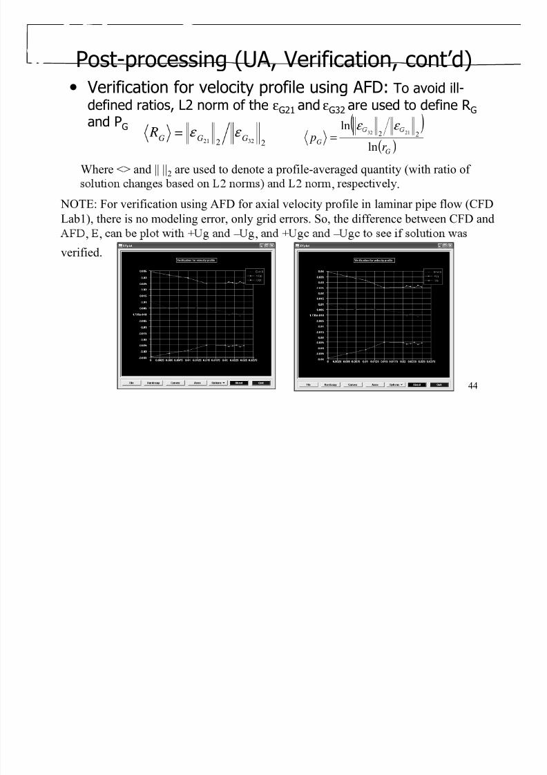
• Verification for velocity profile using AFD: To avoid ill-
defined ratios, L2 norm of the εG21 and εG32 are used to define R Gand PG ln ε ε
22 3221 GGG =( )G
Gr
pln
22 2132
=
Where <> and || ||2 are used to denote a profile-averaged quantity (with ratio of
NOTE: For verification using AFD for axial velocity profile in laminar pipe flow (CFD
Lab1), there is no modeling error, only grid errors. So, the difference between CFD and
+ – + –
, .
, , ,
verified.
44

8/8/2019 Introduction Cfd
http://slidepdf.com/reader/full/introduction-cfd 45/52
Post-processing (UA, Validation)
• Validation procedure: simulation modeling uncertainties
was presented where for successful validation, the comparison
error, , s ess t an t e va at on uncerta nty, v.
• Interpretation of the results of a validation effort
−−V
E U V <
Validation not achieved22
DSN V U U U +=
SN SM D
• Validation example
and validation of wave profile for
series 60
45
Example of CFD Process using CFD
8/8/2019 Introduction Cfd
http://slidepdf.com/reader/full/introduction-cfd 46/52
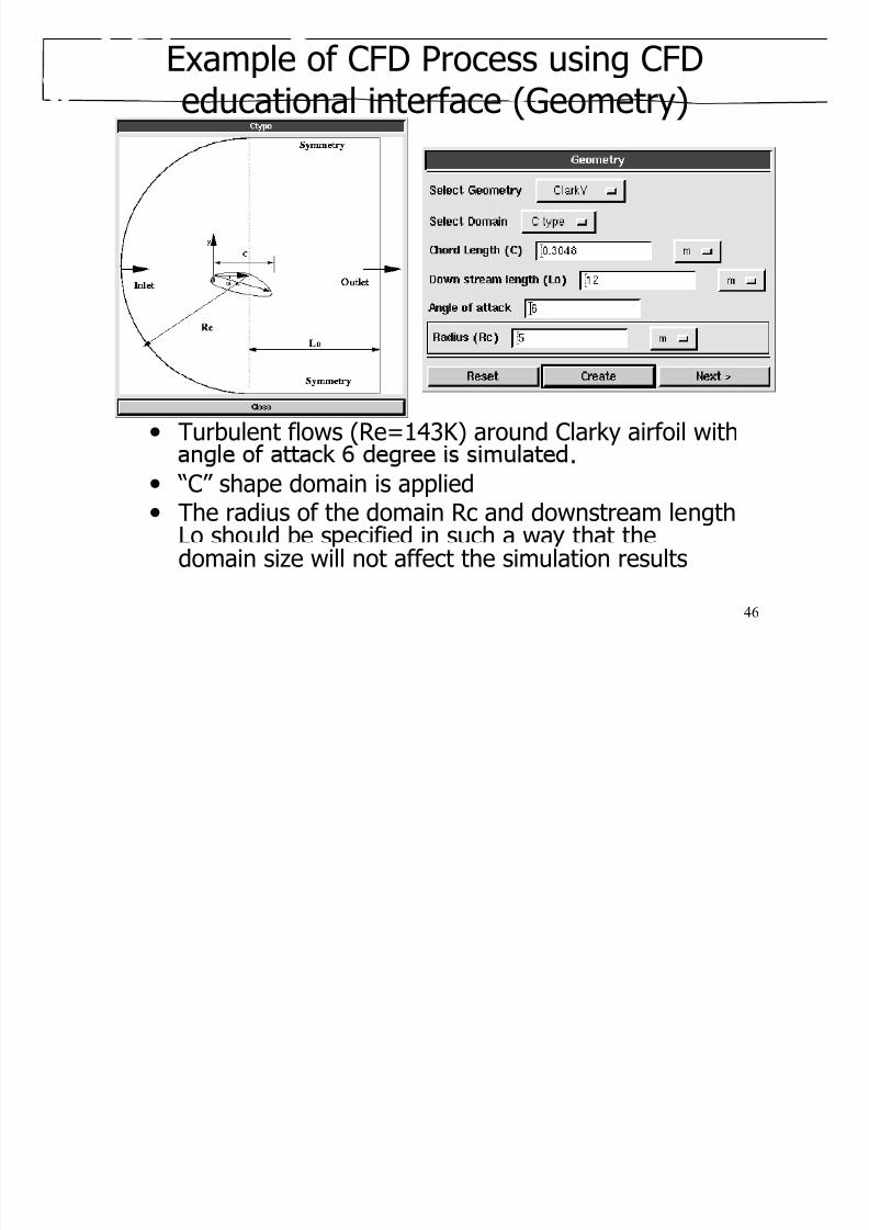
p geducational interface (Geometry)
• Turbulent flows (Re=143K) around Clarky airfoil with.
• “C” shape domain is applied• The radius of the domain Rc and downstream length
Lo should be s ecified in such a wa that the
46
domain size will not affect the simulation results
Example of CFD Process (Physics)
8/8/2019 Introduction Cfd
http://slidepdf.com/reader/full/introduction-cfd 47/52
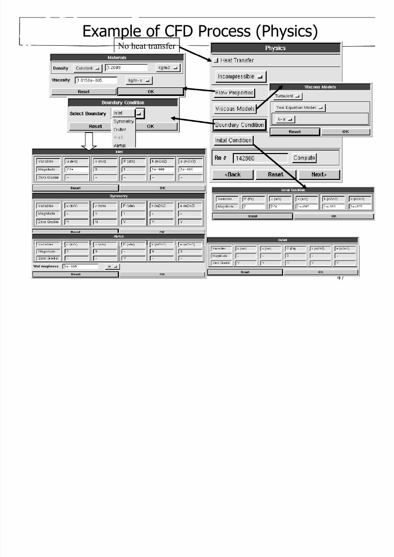
Example of CFD Process (Physics) No heat transfer
47
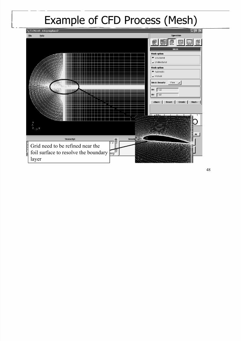
Example of CFD Process (Mesh)
8/8/2019 Introduction Cfd
http://slidepdf.com/reader/full/introduction-cfd 48/52
Example of CFD Process (Mesh)
Grid need to be refined near the
48
foil surface to resolve the boundary
layer
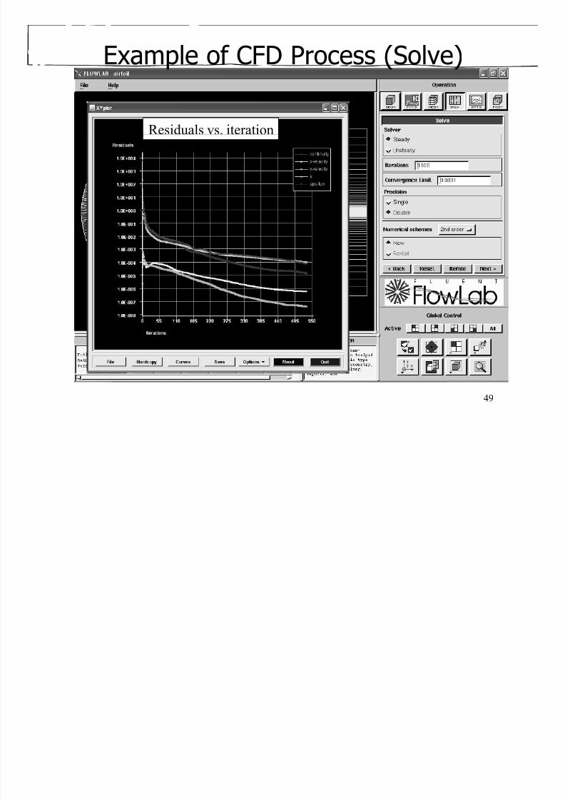
Example of CFD Process (Solve)
8/8/2019 Introduction Cfd
http://slidepdf.com/reader/full/introduction-cfd 49/52
Example of CFD Process (Solve)
Residuals vs. iteration
49
Example of CFD Process (Reports)

8/8/2019 Introduction Cfd
http://slidepdf.com/reader/full/introduction-cfd 50/52
Example of CFD Process (Reports)
50
Example of CFD Process (Post-processing)

8/8/2019 Introduction Cfd
http://slidepdf.com/reader/full/introduction-cfd 51/52
p ( p g)
51
58 160 CFD L b
8/8/2019 Introduction Cfd
http://slidepdf.com/reader/full/introduction-cfd 52/52
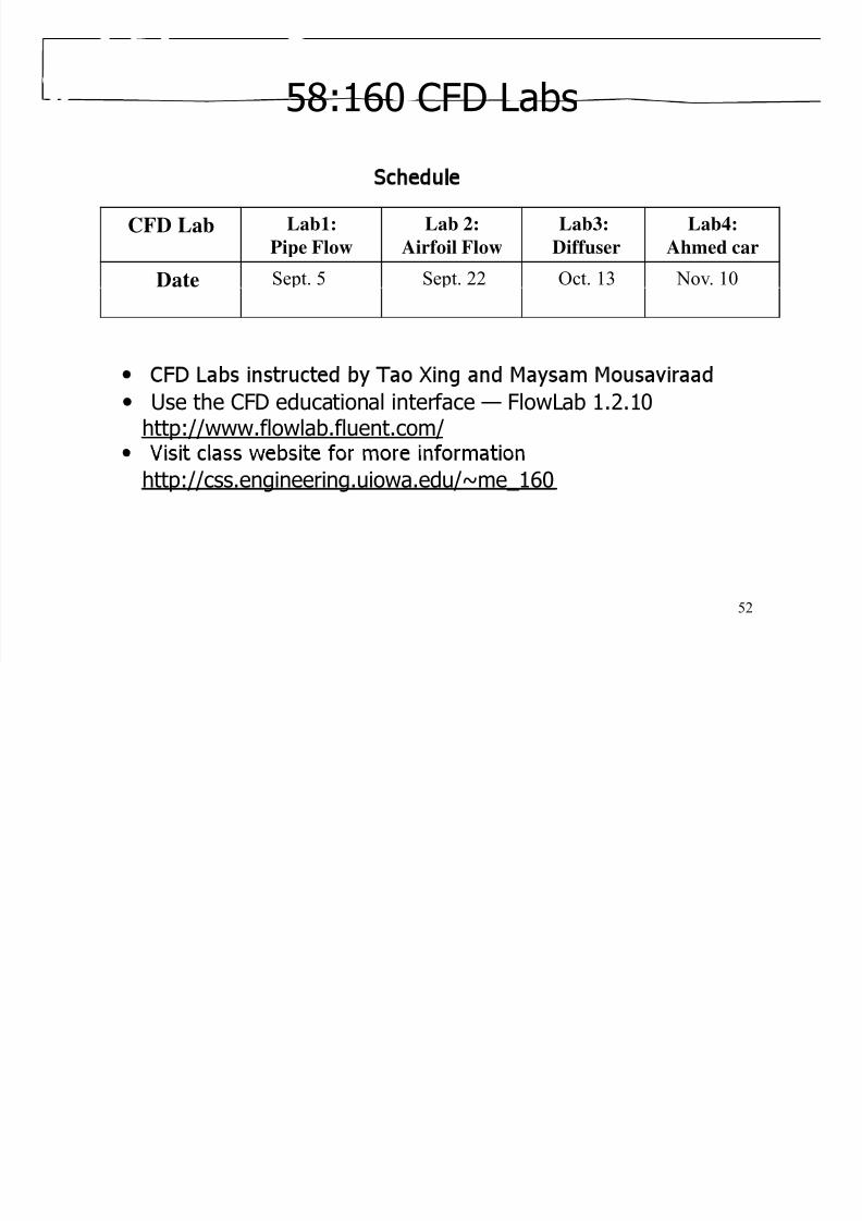
58:160 CFD Labs
Schedule
CFD Lab Lab1:
Pipe Flow
Lab 2:
Airfoil Flow
Lab3:
Diffuser
Lab4:
Ahmed car
Date Sept. 5 Sept. 22 Oct. 13 Nov. 10
• Use the CFD educational interface — FlowLab 1.2.10
http://www.flowlab.fluent.com/
http://css.engineering.uiowa.edu/~me_160
52