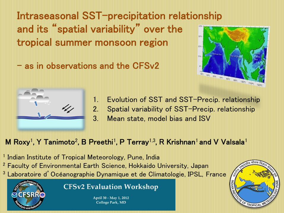
M Roxy1, Y Tanimoto2, B Preethi1, P Terray1,3, R Krishnan1 and V Valsala1

1 Indian Institute of Tropical Meteorology, Pune, India 2 Faculty of Environmental Earth Science, Hokkaido University, Japan 3 Laboratoire d’Océanographie Dynamique et de Climatologie, IPSL, France

1. Evolution of SST and SST-Precip. relationship 2. Spatial variability of SST-Precip. relationship 3. Mean state, model bias and ISV

Intraseasonal SST-precipitation relationship and its “spatial variability” over the tropical summer monsoon region - as in observations and the CFSv2

SST-precipitation relationship in the monsoon ISV; Earlier Studies

1. SST and heat flux anomalies associated with monsoon ISV are observed over a large domain, Arabian Sea -> s. China Sea -> w. North Pacific (Webster et al. 1998; Sengupta et al. 2001; Xie et al. 2007)

2. Intraseasonal SST driven by downward SW radiation flux (dominant) and LHF anomalies.(Hendon & Glick 1997). Over “central Indian Ocean”

3. Intraseasonal SST influence the atmospheric variability, eg: Precipitation (Vecchi and Harrison 2002, Fu et al. 2008). Over “Bay of Bengal”

VH 2002: Negative SST lead monsoon break by 10 days (r = 0.67). Step by step process on the SST- precipitation relationship?

OLR Index

ISV of Bay of Bengal SST (TMI)

(b) SLHF & SST (d) Ftot/ϱcph & SST (e) ∂Ts/∂t & SST (c) DSWRF & SST

SST tendency equation: ∂Ts/∂t = Ftot/ϱcph [where Ts is the SST, Ftot is the total heat flux, ϱ is density of water, cp is the specific heat of water at

constant pressure, and h is the depth of the mixed layer: h = 40 m (Kara et. al 2003)].

Quantitatively: Ftot of 50 Wm-2, h of 40 m, standard ϱ & cp => Ftot/ϱcph = 0.025

oC day-1

SST change of 0.8oC in 40 days => ∂Ts/∂t = 0.02

oC day-1

Arabian Sea (60-70E)

Heat Flux Forcing SST Tendency (a) Zwind & SST

SST-precipitation relationship in the monsoon ISV; Earlier Studies: Evolution of SST

4. Intraseasonal SST over Arabian Sea and Bay of Bengal: driven by both LHF (dominant!) and SWF anomalies (Roxy and Tanimoto 2007, JMSJ).

Easterly Wind Anomalies

Increased Evaporation

moist stat. anomalies

Convective Activity

Ocean

Atmosphere

Easterly Wind Anomalies (reduced total winds)

Reduced Evaporation

Increased SST

∆θe anomalies unstable conditions

Convective Activity

Ocean

Atmosphere

Kemball-Cook & Wang, 2001

Roxy & Tanimoto, 2007

Mean zonal winds are westerly !

(a) SAT & SST (b) ∆θe & SST (c) CLW & SST (d) Precip. & SST

6. positive SST anomalies => destabilize lower atmos. column => convective activity (R & T 2007)

5. Intraseasonal latent heat flux (-ve upward) anomalies enhance precipitation by enhancing the moist static energy (Kemball-Cook and Wang 2001)

Mean profile of virtual potential temperature θv, for 0600 GMT on 2 June (pre-monsoon) and 11-14 June (onset) from MONEX 79 ship data over Arabian Sea. Holt and Raman, 1987.

SST influence on the destabilization of lower atmospheric column: Virtual potential temperature (θv) over Arabian Sea during pre-active phase

Pre

ssure

θ v (oC)

June

Atmospheric soundings between June 2-14

June 11: pre-active phase

(a) θe1000 anomalies (b) θe700 anomalies

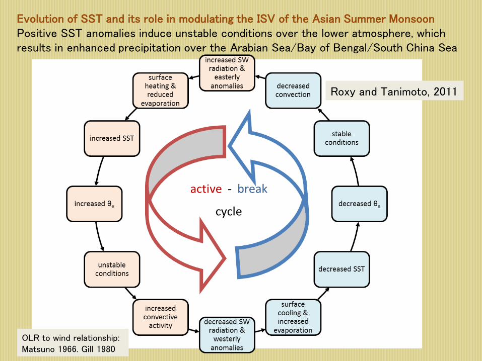
Evolution of SST and its role in modulating the ISV of the Asian Summer Monsoon Positive SST anomalies induce unstable conditions over the lower atmosphere, which results in enhanced precipitation over the Arabian Sea/Bay of Bengal/South China Sea

OLR to wind relationship: Matsuno 1966. Gill 1980

Roxy and Tanimoto, 2011

Atmosphere: NCEP Global Forecast System (GFS) horizontal: spectral T126, ~90 km vertical: 64 sigma-pressure hybrid levels

Ocean: GFDL Modular Ocean Model v4 (MOM4p0) 40 levels in the vertical, 0.25-0.5°horizontal.

Sea Ice: GFDL Sea Ice Simulator (SIS) an interactive, 2 layer sea-ice model

Land: NOAH, an interactive land surface model with 4 soil levels

NCEP CFSv2

SST, Precipitation: TMI Winds: QuickSCAT Fluxes: TropFlux

Observations Data, Model and Methods

1998-2009 (12 years)

~ 100 years simulation with mixing ratios of time varying forcing agents set for the current decade

Anomalies obtained for all variables by removing seasonal means and bandpass filtered for 10-90 days to retain the ISV over the Asian monsoon region, for June-September.

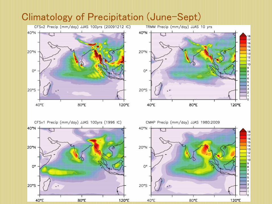
Climatology of Precipitation (June-Sept)

Climatology of Precipitation and SST (June-Sept)

The SST-precipitation relationship have different lead-lags over the Arabian Sea and the Bay of Bengal/South China Sea

Spatial variability of SST – Precipitation relationship

In CFSv2, correlation between SST & precip. is overestimated: TMI rmax= 0.4 CFSv2 rmax= 0.7

(a) TMI

CFSv2 (b)

5 days 12 days

SST –> Precipitation

Bay of Bengal South China Sea

Arabian Sea

The positive SST anomalies translate to positive θe anomalies instantaneously over all the basins, BUT the response in the precipitation anomalies is different.

TMI

CFSv2

Spatial variability of SST – Precipitation relationship

Relatively stronger surface convergence over the Arabian Sea accelerates the uplift of the moist air, resulting in a relatively faster response in the local precipitation anomalies

(a) (b)

ISV of anomalies in Observations and CFSv2 ISV overestimated over the n. Indian Ocean, esp. Arabian Sea

(a) (b)

(c) (d)

(e) (f)

(g) (h)

TMI

CFSv2

Is it due to coupling mismatch? Flux Contribution => SST Tendency

The increased SST anomalies in the model are comparable to the simulated net surface flux anomalies, For 30 W m-2 (30m mld), dT = 0.025C day-1. Wind Contribution => LHF

Using the bulk aerodynamic equations, an overestimation of 1 m s-1 of wind speed is comparable to an increase of 14 W m-2 of latent heat flux anomalies, in the model.

Overestimation of ISV in the CFSv2; model bias

Flux Contribution => SST Tendency

Wind Contribution => LHF

(a) (b) (c) (d)

(e) (f) (g) (h)

ISV of anomalies in Observations and CFSv2 ISV overestimated over the n. Indian Ocean, esp. Arabian Sea

𝜕Ts

𝜕t =

Ftot

ρcp∗𝐌𝐋𝐃

For the same magnitude of fluxes, change in SST is different: Shallow MLD -> ISV amplified Deep MLD -> ISV weakened r = 0.5, significant at 95% levels

JJAS MLD Diff. [CFSv2 - Boyer]

Annual mean MLD difference between model and observations.

Annual mean Temp difference between model and observations (WOA02)

Surface

500m

Indian Ocean cross section

Pacific Ocean cross section

Atlantic Ocean cross section

0C

0C

0C

0C

0C

MLD difference

Annual mean Salinity difference between model and observations (WOA02)

Surface

500m

Indian Ocean cross section

Pacific Ocean cross section

Atlantic Ocean cross section

Surface waves could deliver mixing/turbulences to depth of the order of 100 m directly (Babanin et al. 2009). Some physical processes such as Langmuir circulation and wave-induced vertical mixing have not been properly included in the ocean component, which may be the main reasons for these biases. Langmuir circulation can induce vertical mixing and play an important role in deepening upper-ocean mixed layer (Li et al., 1995; McWilliams and Sullivan, 2000). Besides Langmuir circulation and surface wave breaking, nonbreaking surface waves can also induce vertical mixing in the upper-ocean (Qiao et al., 2004; Dai et al., 2010).

Shu et al 2011, MLD diff. in July, with/without wave induced surface mixing

increased SW radiation &

easterly anomalies decreased

convection

stable conditions

decreased θe

decreased SST

surface cooling & increased evaporation decreased SW

radiation & westerly

anomalies

increased convective

activity

unstable conditions

increased θe

increased SST

surface heating & reduced

evaporation

active - break

cycle

𝜕T

𝜕t ∝

1

MLD

𝜕T

𝜕t ∝

1

MLD response speed

∝ surf. convergence

Roxy et al., 2012 Climate Dynamics Communicated

Response to CO2 in CFSv2