Intradomain RoutingIntradomain Routing

Jennifer RexfordJennifer Rexford

Advanced Computer NetworksAdvanced Computer Networkshttp://www.cs.princeton.edu/courses/archive/fall06/http://www.cs.princeton.edu/courses/archive/fall06/

cos561/cos561/Tuesdays/Thursdays 1:30pm-2:50pmTuesdays/Thursdays 1:30pm-2:50pm

What is Routing?

•A famous quotation from RFC 791 “A name indicates what we seek.An address indicates where it is.A route indicates how we get there.” -- Jon Postel

Forwarding vs. Routing

• Forwarding: data plane– Directing a data packet to an outgoing link– Individual router using a forwarding table

• Routing: control plane– Computing the paths the packets will follow– Routers talking amongst themselves– Individual router creating a forwarding table

Internet Structure

• Federated network of Autonomous Systems– Routers and links controlled by a single entity– Routing between ASes, and within an AS

1

2

3

4

5

67

Web client Web server

Two-Tiered Internet Routing System

• Interdomain routing: between ASes– Routing policies based on business

relationships– No common metrics, and limited cooperation– BGP: policy-based, path-vector routing protocol

• Intradomain routing: within an AS– Shortest-path routing based on link metrics– Routers all managed by a single institution– OSPF and IS-IS: link-state routing protocol– RIP and EIGRP: distance-vector routing protocol

Shortest-Path Routing

• Path-selection model– Destination-based– Minimum hop count or sum of link weights– Dynamic vs. static link weights

32

2

1

14

1

4

5

3

Distance Vector Routing: Bellman-Ford

• Define distances at each node x– dx(y) = cost of least-cost path from x to y

• Update distances based on neighbors– dx(y) = min {c(x,v) + dv(y)} over all

neighbors v

32

2

1

14

1

4

5

3

u

v

w

x

y

z

s

t du(z) = min{c(u,v) + dv(z), c(u,w) + dw(z)}

E.g., RIP and EIGRP

Link-State Routing: Dijsktra’s Algorithm

• Each router keeps track of its incident links– Link cost, and whether the link is up or down

• Each router broadcasts the link state– To give every router a complete view of the graph

• Each router runs Dijkstra’s algorithm– To compute shortest paths and forwarding table

32

2

1

14

1

4

5

3 E.g., OSPF and IS-IS

Routing Protocols (COS 461 #15 and 16)

Link State Distance Vector

Path Vector

Dissem-ination

Flood link state advertisements to all routers

Update distances from neighbors’ distances

Update paths based on neighbors’ paths

Algorithm

Dijsktra’s shortest path

Bellman-Ford shortest path

Local policy to rank paths

Converge

Fast due to flooding

Slow, due to count-to-infinity

Slow, due to path exploration

Protocols

OSPF, IS-IS RIP, EIGRP BGP

History: Packet-Based Load-Sensitive Routing

• Packet-based routing– Forward packets based on forwarding table

• Load-sensitive– Compute table entries based on load or

delay

• Questions– What link metrics to use?– How frequently to update the metrics?– How to propagate the metrics?– How to compute the paths based on

metrics?Still a popular area of research…

Original ARPANET Algorithm (1969)

• Delay-based routing algorithm– Shortest-path routing based on link metrics– Instantaneous queue length plus a constant– Distributed shortest-path algorithm

(Bellman-Ford)

32

2

1

13

1

5

20congested link

Performance of Original ARPANET Algorithm

• Light load– Delay dominated by the constant part

(transmission delay and propagation delay)

• Medium load– Queuing delay is no longer negligible– Moderate traffic shifts to avoid congestion

• Heavy load– Very high metrics on congested links– Busy links look bad to all of the routers– All routers avoid the busy links– Routers may send packets on longer paths

Improvements in the Second ARPANET Algorithm

Original ARPANET Algorithm

(1969)

Second ARPANET Algorithm (1979)

Timescale of the link metric

Instantaneous queue length

Averaging of the link metric over time

Routing protocol

Distance vector slow convergence

Link state for faster convergence

Update frequency

Updates on every metric change

Updates if change passes a threshold

Problem of Long Alternate Paths

• Picking alternate paths– Long path chosen by one router consumes

resource that other packets could have used– Leads other routers to pick other alternate

paths

• Solution: limit path length– Bound the value of the link metric– “This link is busy enough to go two extra hops”

• Extreme case– Limit path selection to the shortest paths– Pick the least-loaded shortest path in the

network

Problem of Out-of-Date Information

• Routers make decisions with old information– Propagation delay in flooding link metrics– Thresholds applied to limit number of updates

• Old information leads to bad decisions– All routers avoid the congested links– … leading to congestion on other links– … and the whole things repeats

Lincoln Tunnel

Holland TunnelNJ NYC

“Backup at Lincoln” on radio triggers congestion at Holland

Intradomain Routing Today

• Link-state routing with static link weights– Static weights: avoid stability problems – Link state: faster reaction to topology changes

• Most common protocols in backbones– OSPF: Open Shortest Path First

– IS-IS: Intermediate System–Intermediate System

• Some use of distance vector in enterprises– RIP: Routing Information Protocol

– EIGRP: Enhanced Interior Gateway Routing Protocol

• Growing use of Multi-Protocol Label Switching

What do Operators Worry About?

• Topology design– Small propagation delay and low congestion– Ability to tolerate node and link failures

• Convergence delay– Limiting the disruptions during topology changes– E.g., by trying to achieve faster convergence

• Traffic engineering– Limiting propagation delay and congestion– E.g., by carefully tuning the “static” link weights

• Scalable routing designs– Avoiding excessive protocol overhead– E.g., by introducing hierarchy in routing

Topology Design: Intra-AS Topology

• Node: router• Edge: link

Hub-and-spoke Backbone

Topology Design: Abilene Internet2 Backbone

Topology Design: Points-of-Presence (PoPs)

• Inter-PoP links– Long distances– High bandwidth

• Intra-PoP links– Short cables between

racks or floors– Aggregated bandwidth

• Links to other networks– Wide range of media

and bandwidth

Intra-PoP

Other networks

Inter-PoP

Convergence: Detecting Topology Changes

• Beaconing– Periodic “hello” messages in both directions– Detect a failure after a few missed “hellos”

• Performance trade-offs– Detection speed– Overhead on link bandwidth and CPU– Likelihood of false detection

“hello”

Convergence: Transient Disruptions

• Inconsistent link-state database– Some routers know about failure before

others– The shortest paths are no longer consistent– Can cause transient forwarding loops

32

2

1

14

1

4

5

3

32

2

1

14

1

4 3

Convergence: Delay for Converging

• Sources of convergence delay– Detection latency– Flooding of link-state information– Shortest-path computation– Creating the forwarding table

• Performance during convergence period– Lost packets due to blackholes and TTL expiry– Looping packets consuming resources– Out-of-order packets reaching the destination

• Very bad for VoIP, online gaming, and video

Convergence: Reducing Convergence Delay

• Faster detection– Smaller hello timers– Link-layer technologies that can detect failures

• Faster flooding– Flooding immediately– Sending link-state packets with high-priority

• Faster computation– Faster processors on the routers– Incremental Dijkstra algorithm

• Faster forwarding-table update– Data structures supporting incremental updates

Traffic Engineering: Tuning Link Weights

32

2

1

13

1

4

5

3

• Problem: congestion along the blue path– Second or third link on the path is overloaded

• Solution: move some traffic to bottom path– E.g., by decreasing the weight of the second link

3

Traffic Engineering: Problem Formulation

• Topology– Connectivity & capacity of routers & links

• Traffic matrix– Offered load between points in the network

• Link weights– Configurable parameters for the protocol

• Performance objective– Balanced load, low latency, service

agreements

• Question: Given topology and traffic matrix, which link weights to use?

Traffic Engineering: Key Ingredients of Approach

• Instrumentation– Topology: monitoring of the routing protocols– Traffic matrix: fine-grained traffic measurement

• Network-wide models– Representations of topology and traffic– “What-if” models of shortest-path routing

• Network optimization– Efficient algorithms to find good configurations– Operational experience to identify key

constraints

Scalability: Overhead of Link-State Protocols

• Protocol overhead depends on the topology– Bandwidth: flooding of link state advertisements – Memory: storing the link-state database– Processing: computing the shortest paths

32

2

1

13

1

4

5

3

Scalability: Improving the Scaling Properties

• Dijkstra’s shortest-path algorithm– Simplest version: O(N2), where N is # of nodes– Better algorithms: O(L*log(N)), where L is #

links– Incremental algorithms: great for small

changes

• Timers to pace operations– Minimum time between LSAs for the same link– Minimum time between path computations

• More resources on the routers– Routers with more CPU and memory

Scalability: Introducing Hierarchy Through Areas

• Divide network into regions– Backbone (area 0) and non-backbone areas– Each area has its own link-state database– Advertise only path distances at area boundaries

Area 0

Area 1 Area 2

Area 3 Area 4

areaborderrouter

Scalability: Dividing into Multiple ASes

• Divide the network into regions– Separate instance of link-state routing per region– Interdomain routing between regions (i.e., BGP)– Loss of visibility into differences within region

100

100

100

100

100

10020 20 20 20 20 20

50

50 50

50

50

50

North America Europe Asia

Limitations of Conventional Intradomain Routing

• Overhead of hop-by-hop forwarding– Large routing tables and expensive look-ups

• Paths depend only on the destination– Rather than differentiating by source or class

• Only the shortest path(s) are used– Even if a longer path has enough resources

• Transient disruptions during convergence– Cannot easily prepare in advance for changes

• Limited control over paths after failure– Depends on the link weights and remaining

graph

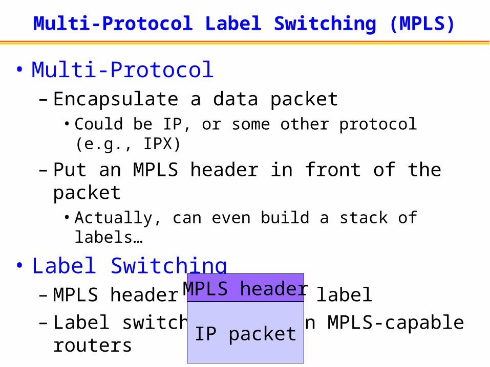
Multi-Protocol Label Switching (MPLS)

• Multi-Protocol– Encapsulate a data packet

• Could be IP, or some other protocol (e.g., IPX)

– Put an MPLS header in front of the packet• Actually, can even build a stack of labels…

• Label Switching– MPLS header includes a label– Label switching between MPLS-capable

routers

IP packet

MPLS header

Multi-Protocol Label Switching (MPLS)

• Key ideas of MPLS– Label-switched path spans group of

routers– Explicit path set-up, including backup

paths– Flexible mapping of data traffic to paths

• Motivating applications– Small routing tables and fast look-ups– Virtual Private Networks– Traffic engineering– Path protection and fast reroute

MPLS: Forwarding Based on Labels

• Hybrid of packet and circuit switching– Logical circuit between a source and

destination– Packets with different labels multiplex on a

link

• Basic idea of label-based forwarding– Packet: fixed length label in the header – Switch: mapping label to an outgoing link

1

2

1: 72: 7

link 7 1: 142: 8

link 14link 8

MPLS: Swapping the Label at Each Hop

• Problem: using label along the whole path– Each path consumes a unique label– Starts to use up all of label space in the

network

• Label swapping– Map the label to a new value at each hop– Table has old label, next link, and new label– Allows reuse of the labels at different links

1

2

1: 7: 202: 7: 53 link 7

20: 14: 7853: 8: 42

link 14link 8

MPLS: Pushing, Swapping, and Popping

IP

Pushing

IP

IPPopping

IP

Swapping

• Pushing: add the initial “in” label• Swapping: map “in” label to “out” label• Popping: remove the “out” label

R2

R1

R3

R4

MPLS core

A

B

C

D

IP edge

MPLS: Forwarding Equivalence Class (FEC)

• Rule for grouping packets– Packets that should be treated the same way– Identified just once, at the edge of the network

• Example FECs– Destination prefix

• Longest-prefix match in forwarding table at entry point

• Useful for conventional destination-based forwarding

– Src/dest address, src/dest port, and protocol• Five-tuple match at entry point• Useful for fine-grain control over the traffic

A label is just a locally-significant identifier for a FEC

Status of MPLS

• Deployed in practice– Small control and data plane overhead in

core– Virtual Private Networks– Traffic engineering and fast reroute

• Challenges– Protocol complexity– Configuration complexity– Difficulty of collecting measurement data

• Continuing evolution– Standards– Operational practices and tools

Conclusion

• Two-tiered Internet routing system– Interdomain: between Autonomous Systems– Intradomain: within an Autonomous System

• Intradomain routing– Shortest path routing based on link metrics– Stability problems with dynamic link metrics– Link-state vs. distance-vector protocols

• MultiProtocol Label Switching (MPLS)– Forwarding packets based on a label– Explicit path set-up