intraday technical trading in the foreign exchange...
TRANSCRIPT

WORKING PAPERS SERIES
WP99-02
Intraday Technical Trading in
the Foreign Exchange Market
Christopher Neely and Paul Weller

Intraday Technical Trading in the Foreign Exchange Market
Christopher J. Neely
Paul A. Weller
Preliminary draft—Not for quotation
September 23, 1999
Abstract: This paper examines the out-of-sample performance of intraday technical trading
strategies selected using two methodologies, a genetic program and an optimized linear
forecasting model. When realistic transaction costs and trading hours are taken into account, we
find no evidence of excess returns to the trading rules derived with either methodology. Thus, our
results are consistent with market efficiency. We do, however, find that the trading rules discover
some remarkably stable patterns in the data.
Keywords: technical trading rules, genetic programming, exchange rates
JEL subject numbers: F31, G15
* Senior Economist, Research Department
Federal Reserve Bank of St. Louis
P.O. Box 442 St. Louis, MO 63166
(314) 444-8568, (314) 444-8731 (fax)
† Department of Finance
Henry B. Tippie College of Business
Administration
University of Iowa
Iowa City, IA 52242
(319) 335-1017, (319) 335-3690 (fax)
The authors thank Kent Koch for excellent research assistance and Olsen and Associates for
supplying the data. Paul Weller would like to thank the Research Department of the Federal
Reserve Bank of St. Louis for its hospitality while he was a Visiting Scholar, when this work was
initiated. The views expressed are those of the author(s) and do not necessarily reflect official
positions of the Federal Reserve Bank of St. Louis or the Federal Reserve System.

1
There has been a recent resurgence of academic interest in the claims of technical analysis.
This is largely attributable to accumulating evidence that technical trading can be profitable over
long time horizons (Brock, Lakonishok and LeBaron, 1992; Levich and Thomas, 1993; Neely,
Weller and Dittmar, 1997)1.
However, academic investigation of technical trading in the foreign exchange market has
not been consistent with the practice of technical analysis. The majority of foreign exchange
traders who use technical analysis are intraday traders who transact at high frequency and aim to
finish the trading day with a net open position of zero. But, due to data limitations, most academic
studies have evaluated the profitability of trading strategies that allow trades to be executed at
most once a day. For example, in our earlier study using daily data (Neely, Weller and Dittmar,
1997), we provide strong evidence for the existence of profitable trading rules for a variety of
currencies over a fifteen-year time horizon. The mean trading frequency for the rules we identify
ranges from once every two weeks to once every three months. Evidently, these are not the
trading strategies being used by the foreign exchange dealers in the London market surveyed in
Taylor and Allen (1992). They documented the fact that technical analysis was widely used for
trading at the shortest time horizons, namely days and weeks, and was used in some form by over
90 per cent of their respondents.2
This paper links trading practice with research more closely by investigating the
performance of trading rules using high frequency data that allow the rules to change position
within the trading day. We use an in-sample period to search for ex ante optimal trading rules and
then assess the performance of those rules out-of-sample. We use two distinct methodologies: the
1 Ready (1998) questions the evidence relating to the equity market.

2
first is a genetic program that can search over a very wide class of (possibly non-linear) trading
rules; the second consists of linear forecasting models. We find strong evidence of predictability in
the data as measured by out-of-sample profitability when transaction costs are set to zero.
However, the excess returns earned by the trading rules are very sensitive to the level of
transaction costs and to the liquidity of the markets. When transaction costs are taken into
account and trading is restricted to periods of high market activity, there is no evidence of
profitable trading opportunities. Thus, our results are consistent with the efficient markets
hypothesis.
2. Previous Work on Trading Rules in the Foreign Exchange Market
Most of the work analyzing technical trading rules in the foreign exchange market has
used daily or weekly data, and has examined the profits to be earned by employing a particular
rule or class of rules suggested by practicing technical analysts. The trading rules that have been
most intensively investigated use filters and moving averages. A simple filter rule takes the form:
“Take a long position in foreign currency when the exchange rate (dollar value of foreign
currency) rises by x% above its previous minimum over the last y days; take a short position when
the exchange rate falls x% below its previous maximum over the last y days. Otherwise maintain
the current position.” A double moving average rule compares a short- to a long-run moving-
average, changing from a sell to a buy signal when the short-run moving average exceeds the
long-run moving average by a given amount. Even these simple rules can take a great variety of
different forms. The moving-average rules will vary depending on the time windows chosen for
2 A more recent survey of foreign exchange traders in the United States (Cheung and Chinn, 1999), although it did
not explicitly address the issue of trading horizon, found that 30 per cent of the sample used technical analysis as
the dominant guide to trading, compared to 25 per cent using fundamental analysis.

3
each moving average and the amount by which the short moving average must exceed or fall
below the long moving average. The filter rules will depend on the size of the filter and the time
window over which the previous high or low is calculated. Both classes of rules seek to identify
changes in a trend.
Curcio et al. (1998) is the only published paper that we are aware of that examines the
profitability of technical trading rules using intraday data. They consider rules that have been
identified by practitioners, rather than developing optimal ex ante rules as we do. They find no
evidence of the existence of profitable trading strategies once transaction costs are taken into
account. A number of studies have examined the performance of particular types of trading rule
using daily foreign exchange data (Dooley and Shafer, 1983; Sweeney, 1986; Levich and Thomas,
1993; Osler and Chang, 1995). The general conclusion is that the trading rules are able to earn
significant excess returns net of transaction costs, and that this cannot be easily explained as
compensation for bearing risk. For example, Neely, Weller and Dittmar (1997) found out-of-
sample annual excess returns in the one to seven percent range in currency markets against the
dollar during the period 1981-95. The highest trading frequency was observed in the rules found
for the DEM/JPY, and was between two and three trades per month. This does not resemble the
technical trading strategies used by most foreign exchange traders. We therefore seek to discover
if the profit opportunities that exist over medium- to long-term horizons are also present at the
short horizons typically employed by traders.
3. The Genetic Program
Genetic algorithms are computer search procedures based on the principles of natural
selection. These procedures were developed by Holland (1975) and extended by Koza (1992).

4
They have been applied to a wide variety of problems in many fields and are most useful in
situations where the space of possible solutions to a problem consists of decision trees or
programs and thus cannot be handled by hill-climbing search routines that require differentiability.
Our use of the genetic program follows an approach first applied to the foreign exchange market
in our earlier paper. Our description of the procedures used here will follow that of the previous
paper.
In genetic programming, the individual candidate solutions are hierarchical character
strings of variable length. These structures can be represented as decision trees, whose non-
terminal nodes are mathematical functions, operators or constants. We make use of the following
function set:
• arithmetic operations: “plus”, “minus”, “times”, “divide”, “norm”, “average”, “max”,
“min”, “lag”;
• Boolean operations: “and”, “or”, “not” ”, “greater than”, “less than”;
• conditional operations: “if-then”, “if-then-else”;
• random numerical constants picked uniformly from (0,6);
• Boolean constants: “true”, “false”.
“Norm” returns the absolute value of the difference between two numbers. “average”, “max”,
“min”, and “lag” respectively return the moving average, local maximum, local minimum and
lagged value of a data series over a time window specified by the argument of the function,
rounded to the nearest whole number.
We use three information variables as input to the genetic program. The first is the
normalized value of the exchange rate, the exchange rate divided by its moving average over the

5
previous two weeks.3 The second summarizes information on the interest differential, and is
defined in the section describing the data. The third variable is the hour of the day. We include this
last variable because of the large and consistent intraday fluctuation in trading volume in foreign
exchange markets. This is known to be associated with volatility, but may also have an effect on
the first moment of the exchange rate series.
The genetic program searches for good solutions to problems of interest using the
principles of natural selection. The program first randomly creates a population of arbitrary rules
and allows the members of that population to reproduce and recombine their components over
subsequent generations. Profitable rules are more likely to have their components reproduced in
subsequent populations. In this way, the genetic program searches through the space of rules,
concentrating on those parts of the space that have been shown to produce profitable rules. The
basic features of the genetic program are (a) a means of encoding trading rules so that they can be
built up from separate subcomponents (b) a measure of excess return or “fitness” (c) an operation
which splits and recombines existing rules in order to create new rules.
We denote the exchange rate at period t (dollars per unit of foreign currency) by St , the
short term interest differential by Dt and time of day at period t by the variable, Tt. A trading rule
is a mapping from past exchange rates and interest differentials indexed by time of day to a binary
variable, zt , which takes the value +1 for a long position in foreign exchange at time t, and -1 for
a short position. Trading rules may be represented as trees, whose nodes consist of various
arithmetic functions, logical operators and constants. The functions are distinguished by the data
3 It is useful to divide the exchange rate by a suitable moving average to provide the rules with similar magnitudes
of data both in and out of sample. For example, a rule comparing the exchange rate to a constant in the in-sample
period could perform poorly because the constant was of inappropriate magnitude out of sample. This could come
about as a result of non-stationarities in the data.

6
series on which they operate. Thus max ( )S 3 at time t is equivalent to ( )21,,max !! ttt SSS , lagT(3)
at time t is equal to Tt-3, and averageS(3) is equal to the mean of St, , St - 1 and St -2.
Figure 1 presents an example of a trading rule that makes use of both exchange rate and
time of day data. The rule signals a long position in foreign currency if the current exchange rate
is greater than the 48-period moving average and the time of day (GMT) is between 0800 and
1600, and a short position otherwise. This example illustrates a simple, time-dependent rule. The
function “rate” returns the average of bid and ask quotes for the exchange rate at half-hourly
intervals.
The fitness criterion for the genetic program is the continuously compounded excess
return to the trading rule over the given time period. We train rules under two assumptions about
when they can trade. The first scenario permits trading 24 hours a day, 7 days a week. The
second scenario—called restricted trading—only permits trading during 12-hour periods of heavy
trading in the particular currency on business days. After the 12 hours of trading, the rule earns
the overnight interest rate in the currency in which it is long—losing the overnight interest rate in
the other currency. The continuously compounded (log) excess return over a half-hour is given
by ztrt where zt is the indicator variable described above, and rt is defined as:
r S St t t= !+ln ln1 . (1)
Each trade involves switching from a long to a short position or vice versa, and so incurs a round
trip transaction cost. In other words, trading from a position long x units of foreign currency to
one short the same amount requires a sale of 2x units, incurring a proportional transaction cost of

7
2c. Therefore the cumulative excess return r for a 24-hour trading rule giving signal zt at time t
over the period from time zero to time T is:
( )cnrzrT
t
tt 21ln1
0
!+="!
=
. (2)
where n is the number of trades. This measures the fitness of the rule. Returns to rules subject to
restricted trading would be computed using the interest differential for overnight positions as well
as the exchange rate return.
Figure 2 illustrates the crossover and reproduction operation. A pair of rules is selected at
random from the population, with a probability weighted in favor of rules with higher fitness.
Then subtrees of the two parent rules are selected randomly. One of the selected subtrees is
discarded, and replaced by the other subtree, to produce the offspring rule.4
To implement the genetic programming procedures we define 3 separate subsamples,
referred to as the training, selection and out-of-sample test periods. The first two periods are
equivalent to an in-sample estimation period. The third, the out-of-sample test period, is used to
measure the performance of the rules trained and selected in the first two periods. The distinct
time periods for all currencies were chosen as follows: training period, 02/01/96 to 03/31/96;
selection period, 04/01/96 to 05/31/96; test period, 06/01/96 to 12/31/96. The first month of data
was used to calculate starting values for moving averages and other functions taking lagged
values as arguments.
The separate steps involved in implementing the genetic program are detailed below.

8
1. Create an initial generation of 1000 randomly generated rules.
2. Measure the excess return of each rule over the training period and rank according to
excess return.
3. Select the top-ranked rule and calculate its excess return over the selection period. If it
generates a positive excess return, save it as the initial best rule. Otherwise, designate the no-trade
rule as the initial best rule, with zero excess return.
4. Select two rules at random from the initial generation, using weights attaching higher
probability to more highly-ranked rules. Apply the reproduction operator to create a new rule,
which then replaces an old rule, chosen using weights attaching higher probability to less highly-
ranked rules. Repeat this procedure 1000 times to create a new generation of rules.
5. Measure the fitness of each rule in the new generation over the training period. Take the
best rule in the training period and measure its fitness over the selection period. If it outperforms
the previous best rule, save it as the new best rule of the second generation.
6. Return to step 4 and repeat until we have produced 40 generations or until no new best
rule appears for 10 generations.
4. The Linear Forecasting Model
We estimate an autoregressive model for each exchange rate over the training and
selection periods on 24-hour data, including weekends, using only own lagged values of the log
exchange rate. We restrict the maximum number of lags to 10. We then combine each estimated
forecasting model with a filter to produce a trading rule. Denoting the one-period-ahead forecast
4 The operation is subject to the restriction that the resulting rule must be well-defined, and that it may not exceed

9
of the log exchange rate at time t by ( ))ln( 1+tt SE and the filter by f, trading signals are determined
in the following way:
( )
( )
( )( ) .ln)ln( if ,1
,ln)ln( if ,1 ,1 If
.ln)ln( if ,1
,ln)ln(if ,1 ,1 If
1
11
1
11
fSSE
fSSEzz
fSSE
fSS Ezz
ttt
ttttt
ttt
ttttt
+#!=
+>+=!=
!$+=
!<!=+=
+
+!
+
+!
(3)
Trading rules with filters ranging from zero to 0.0005 in steps of 0.0001 and estimated lag
coefficients from one to ten are run on the data from the training and selection periods, and excess
return is calculated assuming the following three values of one-way transaction cost: 0, 0.0001,
and 0.0002. The trading rule with the highest excess return for each of the three levels of
transactions cost is then run on the out-of-sample test period.
We also estimate an expanded model in which in addition to the lagged values of the log
exchange rate we include the lagged normalized exchange rate, the hour of the day and the
interest futures differential. Trading rules are then formed in the same way, tested in-sample over
the same range of lags and filters and run on the test period.
5. The Data
We use half-hourly bid and ask quotes for spot foreign exchange rates during 1996 from
the HFDF96 data set provided by Olsen and Associates. We examine four currencies against the
dollar – the German mark (DEM), the Japanese yen (JPY), the British pound (GBP) and the
Swiss franc (CHF). We use three variables as input to the genetic program. The first is the
normalized half-hourly exchange rate series, constructed by calculating a simple average of bid
a specified size (10 levels and 100 nodes).

10
and ask quotes and dividing by a two-week moving average. The second is the difference (U.S.
minus foreign contract) in the transaction prices for the short-term interest rate futures contract
whose expiry is closest to the time stamp of the exchange rate data. The U.S. contract is traded
on the Chicago Mercantile Exchange. Data for the foreign contracts comes from the London
International Financial Futures Exchange (LIFFE). The third variable is the time of day (GMT).
We present summary statistics for the distributions of half-hourly log exchange rate
changes in Table 1. Standard deviations are quite similar across currencies, and all exchange rates
display very high kurtosis. In the top panel of Figure 3 we plot autocorrelations for the log
returns, using all hours, and find highly significant negative first order autocorrelation for all
currencies.5 This significant first-order autocorrelation is also present in both bid and ask prices
and it is robust to excluding outliers in the bid-ask spread. We checked to see whether the
summary statistics or autocorrelation patterns were sensitive to the omission of weekends or off-
peak trading hours. The bottom panel of Figure 3 shows that measuring autocorrelation only
during business hours reduces mean first-order autocorrelation to -0.12, from -0.17 when
measured during all hours. There was also a decline in kurtosis as more periods of low market
activity were omitted. However the kurtosis still remained highly significant in all cases.
Baillie and Bollerslev (1991) note the existence of significant negative first order serial
correlation in hourly exchange rate series, and suggest that it is a spurious consequence of two
features of the data collection process. They used a data set in which each observation consisted
of the average of the five most recent bid quotes, a procedure known to induce serial correlation.
5 It is interesting to compare this result with the findings of Bollerslev and Domowitz (1993). Using observations
on percentage changes at five-minute intervals in the USD/DEM market they report positive third-order
autocorrelation when the series is constructed either from the average of bid and ask quotes or from an algorithm
approximating transaction prices. Thus the pattern of momentum and reversal documented at longer time horizons
in equity markets appears here at much shorter horizons.

11
However this is not a feature of the data set that we use, and so we consider the second reason
they propose—non-synchronous trading. If there are periods during which no trade occurs, and a
zero return is recorded, this may not be an accurate reflection of the movement of the true
underlying return process. When a trade occurs after a period of inactivity, the observed return is
a sum of the accumulated returns over the periods of no trade. If the series has a non-zero mean,
this will induce mean reversion in the observed series. The first point to make is that quotes may
adjust even when no trade takes place, so it is unclear to what extent the argument applies to our
data set. However, we do find a rather high proportion of zero returns in the full sample, ranging
across the four currencies from 22 to 26 per cent of the total number of observations. This is
almost entirely due to the presence of weekends, and the figures fall to a range of 3.9 to 5.9 per
cent when weekends are excluded and further when only business hours are considered.
Lo and MacKinlay (1990) derive a formula for the level of serial correlation induced by
non-synchronous trading if the true return series follows a random walk with drift. It depends on
the mean and variance of the return series, and the probability of no trade occurring. We use the
sample proportion of zero return observations as a proxy for the probability of no trade occurring.
If true returns are generated by the model
ttr !µ += (4)
where t! is a noise term with zero mean and variance 2" independent at all leads and lags, and
# is the probability of no trade, then ( )i$ , the induced correlation in observed returns o
tr at lag i
is given by
( )22
2
1
2µ
#
#"
#µ$
!+
!=
i
i . (5)

12
We obtain a figure for ( )1$ of –0.00000706 for the DEM even when the probability of no
trade is set to 0.227. This is to be compared with the observed value of –0.14. We conclude that
the magnitude of serial correlation observed in the data cannot be explained by non-synchronous
trading, and treat it as a true feature of the data and not an artifact.
6. Results
We consider first the unrestricted, benchmark case in which trading is allowed to take
place twenty-four hours a day, seven days a week. For each currency we generated twenty-five
rules from the genetic program under each of three assumptions about transactions costs in
training and selection periods. We used one-way transaction costs of zero, one and two basis
points (c = 0, 0.0001, 0.0002).6 From those twenty-five rules we selected those which had a
positive excess return during the selection period and also traded at least once.
We aggregate the signals from the sets of individual rules by constructing an equally
weighted portfolio rule. The equally weighted portfolio rule assumes that the trader permits each
rule an equal share in the position taken by the portfolio. Table 2 presents results for this rule. To
investigate pure predictability—as opposed to profitability—in column three we report annual
returns assuming zero transaction costs in the out-of-sample period. To indicate the potential
profitability (or lack thereof) of these rules, column six of Table 2 reports the level of transaction
cost measured in basis points that would reduce the excess return to zero (break-even transaction
cost). The rules trained with zero transactions costs in-sample produce returns that are very high,
in three of the four cases over 100 per cent per annum. This provides strong evidence of a
6 We chose not to compute rules for higher levels of transaction cost because of the increasing difficulty of finding
rules that were profitable in-sample using higher levels of costs. In addition, estimates of foreign exchange

13
predictable component in the exchange rate series. But the rules trade very frequently,
approximately once an hour on average, or every other period. Because of this, the break-even
transaction cost is low. The highest figure among the four exchange rates, that for the British
pound, is 1.01 basis points for a one-way trade. This is largely attributable to the somewhat lower
trading frequency of these rules.
As the transaction cost in training and selection periods is increased from zero to one and
then two basis points, both annual excess returns before transaction cost and trading frequency
fall sharply. But break-even transaction cost rises uniformly to levels close to the level that a large
institutional trader would face. It also becomes more difficult to find good rules according to our
in-sample selection criteria, most notably in the case of the GBP, where only five of the twenty-
five rules satisfied the criteria for c = 0.0002. One of the most striking features of Table 2 is the
steady rise in break-even transaction cost as the in-sample value of c is increased.7 Since the
break-even transaction cost can be interpreted as the average excess return per zero-cost trade,
this demonstrates the ability of the search procedure to identify rules that can successfully predict
not just the direction but also the magnitude of a price change. It also shows that there are
remarkably stable patterns in the high frequency data. Although a purely speculative trader cannot
exploit these patterns, they nevertheless represent important information for foreign exchange
dealers. A dealer who takes account of the predictability in the exchange rate in setting quotes will
trade more profitably than one who does not.
transaction costs suggest that 2-2.5 basis points for a one-way trade is realistic for recent large transactions (Neely,
Weller and Dittmar, 1997).7 The number of trades and breakeven transaction cost for the equally weighted rule are not simple averages over
all rules. We correct for the fact that if two rules simultaneously trade in opposite directions, this has no effect on
the net open position and so does not generate a trade.

14
We can investigate more systematically the role played by serial correlation in the data by
comparing the performance of the linear (autoregressive) forecasting model with that of the
genetic program. Table 3 reports the estimated coefficients of the models with the highest excess
return (net of one-way transaction costs of 0.0001) over training and selection periods. As the
statistics on serial correlation would lead one to expect, the first two lags in the data are much the
most important in all cases. Only the model for the GBP has more than three lags and the
coefficients on lags four and higher are small. The implied models for the log exchange rates are
(barely) stationary. The optimally selected filters for all currencies are 0.0001, matching the
chosen level of transaction cost. When we consider the out-of-sample performance of the
autoregressive forecasting model (see Table 4) we see a similar pattern of improvement as the in-
sample transaction cost increases. However, the results are clearly superior to those derived from
the genetic program at the highest level of transaction cost. In all cases the break-even transaction
cost is higher, dramatically so in the case of the DEM, where it is 24.4 basis points. If we take 2.5
basis points as an estimate of the one-way transaction cost faced by a large institutional trader,
then the trading rules earn excess returns net of transaction cost which in all cases exceed twenty
per cent per annum. However, it is not clear that this is a reasonable thing to do given that we
have assumed that trading takes place twenty four hours a day and during weekends. There are
periods during the week when the major markets are closed and trading activity is much reduced.
The fall in liquidity is very likely to be associated with an increase in transaction cost.
For this reason we generate a new set of rules under the assumption that trading is
restricted to occur during a twelve-hour period on weekdays only. Such rules were able to
observe both business and non-business data but were only permitted to change positions during
business hours. During non-business hours the rules earned or lost the appropriate interest

15
differential. We selected the business hours to coincide with the time of the most active trading in
the particular currency (see Melvin, 1997 for figures on the DEM). They were chosen as follows:
DEM 0600-1800 GMT, JPY 0400-1600 GMT, CHF 0500-1700 GMT, GBP 0500-1700 GMT.
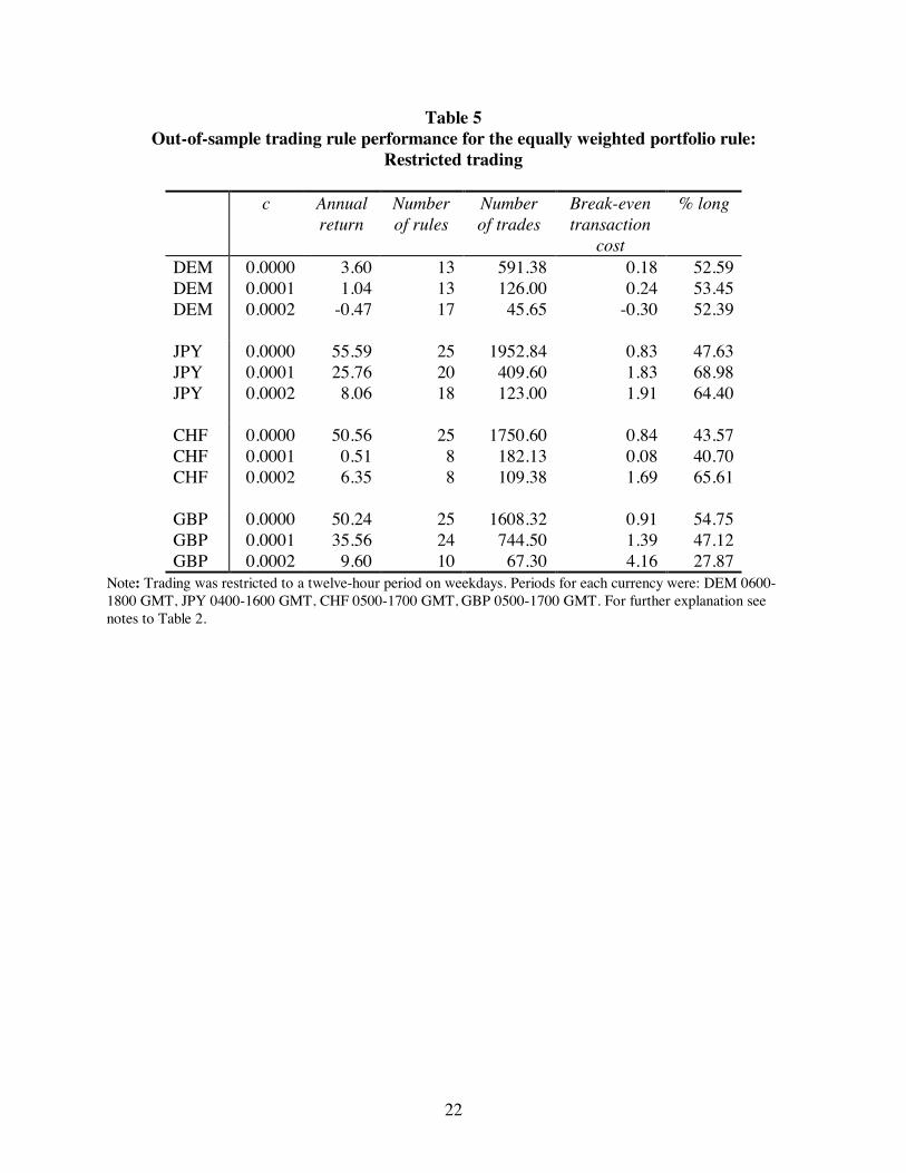
The results for the genetic program with restricted trading are presented in Table 5. The
annual excess returns with zero transactions costs are reduced in close proportion to the reduction
in trading time for all currencies except the DEM. There is still strong evidence of predictability
for these currencies. Break-even transaction costs are generally reduced to a level below that
which an institutional trader would face. The only exception to this is the GBP, where for c =
0.0002 we find a break-even transaction cost of 4.2 basis points. One should be cautious about
reading too much into this finding. There were a relatively small number of good rules identified
in sample, they traded infrequently and tended to be skewed towards short positions.8
In Table 6 we show the results of imposing restricted trading on the autoregressive-
forecasting model. Again, the models are estimated on 24-hour, in-sample data but are only
permitted to change positions during business hours. During non-business hours, the models earn
or lose the appropriate interest differential. The model with the highest excess return net of
transaction costs is then tested out of sample. The picture changes dramatically when compared
to the figures in Table 4. In all cases in which the rules trade, the break-even transaction costs fall
to a level below that which even a large trader would face. This demonstrates conclusively that
the apparent profitability of the trading rules obtained with c = 0.0002 is solely attributable to
trading during periods of reduced market activity when transaction costs are likely to be
substantially higher than the benchmark figure of 2.5 basis points that we have chosen.
8 We also computed results for the case where rules trained on 24-hour data were used for restricted trading out of
sample. Thus, whatever position was signaled by the rule at the beginning of the no-trade period was held until

16
The results from the rules derived from the extended linear forecasting model with
additional variables were not significantly different from the autoregressive results reported in
Table 4, and so we omit them. This indicates that there is no additional forecasting power
contained in the variables added in the extended model%exchange rate normalized by a two-week
moving average, time of day and interest differential.
Tables 6 and 7 summarize the extent to which the genetic program rules find common
patterns during the out-of-sample test period. For each observation we calculate the proportion of
rules which signal a long position and then count how often the proportion of long rules lies in
each quintile. For example, the first entry in the third column of Table 6 indicates that for 50.6
percent of the observations, 0 to 20 percent of the all-day DEM rules with c = 0 were long in the
DEM. That is, a more than 80 percent of the rules were simultaneously short the DEM over half
the time. High numbers in the first and last quintiles indicate consensus among the rules. If there
were no predictable patterns in the data, the trading rules would switch randomly between long
and short positions and we would tend to observe a high percentage of observations in the middle
quintile. We observe the highest degree of consensus in the all-day trading scenario with zero
transaction cost. There is a general tendency for consensus to decline as transaction costs are
increased.
The fact that the trading rules identified by the genetic program generally perform less well
than those generated by the autoregressive-forecasting model deserves some comment. This is
likely to be attributable to two factors. First, the variables in addition to the exchange rate series
that were provided as input to the genetic program proved not to be informative. This is
trade was allowed to start again. The returns of the rules were in almost all cases inferior to those reported in Table
5 and we do not include them.

17
suggested by the fact that the inclusion of these variables in the forecasting model did not make
any difference.9 We have found in our previous work that the inclusion of uninformative data can
degrade the efficiency of the genetic program. Second, if the relevant information enters the
model in a linear fashion, then confining the search to the set of linear models will be a more
efficient procedure.
7. Discussion and Conclusion
Our findings demonstrate that there are very stable predictable components to the intraday
dollar exchange rate series for all the currencies we consider, German mark, Japanese yen, Swiss
franc and British pound. But neither the trading rules identified by the genetic program nor those
based on the linear forecasting model produce positive excess returns once reasonable transaction
costs are taken into account and trade is restricted to take place during times of higher market
activity. The rules based on the autoregressive forecasting model perform at least as well as those
found by the genetic program and the extended linear model, indicating that our results are largely
attributable to the low order negative serial correlation in the data. Previous authors (e.g. Baillie
and Bollerslev, 1991) have suggested that this serial correlation is an artifact that can be explained
by non-synchronous trading. We show that this is not the case for our data set.
A striking feature of our results is that the break-even transaction costs generally converge
to a level close to that faced by a large institutional trader, namely two to three basis points per
one-way trade. These conclusions are based on an analysis of round-the-clock trading. If we
9 We confirmed this fact for the case of the genetic program rules by conducting various experiments in which the
separate data series were randomized separately and changes in out-of-sample performance for the rules were
recorded. No significant impact was observed for any series but the exchange rate.

18
restrict trading to occur during a twelve-hour window of high volume, break-even transaction
costs are considerably reduced.
Our findings are consistent with those of Lyons (1998). He examined the trading behavior
of a foreign exchange dealer over the course of a week, using data that enabled him to decompose
profits into speculative and non-speculative components. He found that he could attribute less
than ten per cent of profits to speculation and that the vast majority came from trading off the
spread.
It is interesting that the foreign exchange market seems to display quite different
characteristics depending on the trading horizon. At weekly and monthly horizons there is strong
evidence to indicate significant and persistent trends, but, as we show here, this is not the case at
intraday horizons. This may be a consequence of the uneven division of capital allocated to
financing trade at different horizons. Although no precise figures are available, there is little doubt
that a much greater volume of transactions is accounted for by traders who close their positions at
the end of each day than by those who take open positions with horizons of weeks or months.
19
References
Allen, Franklin and Risto Karjalainen, 1998. "Using Genetic Algorithms to Find Technical
Trading Rules," Journal of Financial Economics 51, p. 245-271.
Baillie, Richard T. and Tim Bollerslev, 1991, “Intra-day and inter-market volatility in foreign
exchange rates,” Review of Economic Studies 58, 565-585.
Bollerslev, Tim and Ian Domowitz, “Trading Patterns and Prices in the Interbank Foreign
Exchange Market,” Journal of Finance, 48(4), September 1993, 1421-1443.
Brock, William, Josef Lakonishok, and Blake LeBaron. "Simple Technical Trading Rules and the
Stochastic Properties of Stock Returns," Journal of Finance; 47(5), December 1992,
pages 1731-64.
Cheung, Yin-Wong and Menzie D. Chinn, “Macroeconomic Implications of the Beliefs and
Behavior of Foreign Exchange Traders,” Working Paper, Department of Economics,
University of Santa Cruz, January 1999.
Curcio, Riccardo, Charles Goodhart, Dominique Guillaume and Richard Payne, “Do Technical
Trading Rules Generate Profits? Conclusions from the Intra-Day Foreign Exchange
Market,” Journal of Financial and Quantitative Analysis (September 1998), p. 383-408.
Dooley, Michael P. and Jeffrey R. Shafer. “Analysis of short-run exchange rate behavior: March
1973 to November 1981.” In Exchange rate and trade instability: causes, consequences,
and remedies, D. Bigman and T. Taya, eds. Cambridge, MA: Ballinger (1983).
Holland, John. Adaptation in Natural and Artificial Systems, Ann Arbor, MI: University of
Michigan Press (1975).
Koza, John R. Genetic Programming: On the Programming of Computers by Means of Natural
Selection, Cambridge, MA: MIT Press (1992).
Levich Richard and L. Thomas. “The Significance of Technical Trading Rule Profits in The
Foreign Exchange Market: A Bootstrap Approach.” Journal of International Money and
Finance, 12 (October 1993), 451-74.
Lyons, Richard K., “Profits and Position Control: A Week of FX Dealing,” Journal of
International Money and Finance 17, 1998, 97-115.
Melvin, Michael. International Money and Finance, Fifth Edition, Reading, MA: Addison Wesley
Publishing (1997)
Neely, Christopher J. and Paul A. Weller, "Technical Analysis and Central Bank Intervention."
FRB St. Louis Working Paper 97-002B, revised March 1999.
Neely, Christopher J. and Paul A. Weller, "Technical Trading Rules in the European Monetary
System." Journal of International Money and Finance (June 1999), 429-58.
Neely, Christopher J., Paul A. Weller and Robert Dittmar, "Is Technical Analysis in the Foreign
Exchange Market Profitable? A Genetic Programming Approach." Journal of Financial
and Quantitative Analysis (December 1997), 405-26.
Ready, Mark J., "Profits from Technical Trading Rules," unpublished manuscript, University of
Wisconsin, July 1998.
Osler, Carol L. and P. H. Kevin Chang. “Head and Shoulders: Not Just a Flaky Pattern.” Staff
Papers No. 4, Federal Reserve Bank of New York (August 1995).
Sweeney, Richard J. “Beating the foreign exchange market.” Journal of Finance, 41 (March
1986), 163-82.
Taylor, Mark P. and Helen Allen. “The use of technical analysis in the foreign exchange market.”
Journal of International Money and Finance, 11 (June 1992), 304-14.

20
Table 1
Summary statistics
Mean Std. Dev. Skew Kurt ( )1$ ( )2$ ( )3$ Min Max
DEM 0.00022 0.07189 -0.07 25.64 -0.14 -0.03 -0.01 -0.93 0.97
JPY 0.00050 0.07939 -0.05 14.16 -0.17 -0.02 0.00 -0.90 0.92
CHF 0.00063 0.09339 -0.23 31.73 -0.17 -0.01 -0.01 -1.59 1.62
GBP -0.00071 0.07041 0.27 34.14 -0.19 -0.03 -0.02 -1.20 1.22
Note: the table presents statistics for log exchange rate changes constructed from the full data set, consisting of
16080 half-hourly observations (average of bid and ask) taken 24 hours a day, seven days a week for the year 1996.
Mean and standard deviation are multiplied by 100. The skewness and kurtosis statistics are standard normally
distributed. ( )i$ records the autocorrelation coefficient at lag i. Min and max record the smallest and largest half-
hourly percentage changes over the sample period.
Table 2
Out-of-sample trading rule performance for the equally weighted portfolio rule:
All-day trading
c Annual
return
Number
of rules
Number
of trades
Break-even
transaction
cost
% long Long
return
DEM
DEM
DEM
0.0000
0.0001
0.0002
66.92
46.09
6.30
25
21
19
4908.76
887.57
88.58
0.40
1.51
2.08
45.69
60.19
54.46
2.30
JPY
JPY
JPY
0.0000
0.0001
0.0002
130.56
43.28
16.30
25
23
13
4164.44
451.57
144.69
0.91
2.80
3.28
48.40
45.30
60.33
11.72
CHF
CHF
CHF
0.0000
0.0001
0.0002
127.48
92.40
30.99
25
25
15
4846.88
1773.96
388.60
0.77
1.52
2.33
50.02
50.46
45.98
11.51
GBP
GBP
GBP
0.0000
0.0001
0.0002
132.34
111.18
31.59
25
25
5
3830.92
1920.96
412.00
1.01
1.69
2.24
49.62
48.49
63.60
-15.80
Note: the equally weighted portfolio rule attaches a weight (1/# of rules) to each rule satisfying the selection
criteria. Column 2 records the value of c, the one-way transaction cost used in training and selection periods.
Column 3 gives the annualized per cent excess return over the seven-month out-of-sample test period calculated
assuming zero transaction cost. Column 4 reports the number of rules out of the twenty-five obtained for each case
that produced a positive excess return before transactions costs and also traded. These were the rules used for the
out-of-sample test. Number of trades reports the number of trades corrected for double counting. Break-even
transaction cost is the one-way transaction cost (in basis points) which reduces the annual excess return during the
test period to zero. % long is the average percentage of the test period the rules held a position long the foreign
currency. Long return gives the annualized excess return to a long position in the currency held throughout the
out-of-sample test period (buy-and-hold return).

21
Table 3
Estimated coefficients for the optimal linear forecasting model: c = 0.0001
Lag 1 2 3 4 5 6 7 8 9 const f
DEM 0.89 0.11 0.0003 0.0001
JPY 0.85 0.15 0.0115 0.0001
CHF 0.77 0.18 0.05 0.0001 0.0001
GBP 0.78 0.16 0.05 0.00 0.01 0.02 -0.03 -0.01 0.02 -0.0009 0.0001
Note: columns 2 to 10 give the estimated lag coefficient for the best performing model over training and selection
periods when one-way transaction cost was 0.0001. Column 11 records the constant and column 12 the optimal
filter. Presenting more digits would show that all of the models imply stationary ARMA processes for the log
exchange rate.
Table 4
Out-of-sample trading rule performance for the linear forecasting model
All-day trading
c Annual
Return
Number
of trades
Break-even
transaction
cost
% long
DEM 0.0000 92.68 3847 0.71 0.42
DEM 0.0001 79.30 640 3.63 0.37
DEM 0.0002 30.75 37 24.37 0.40
JPY 0.0000 94.28 2304 1.20 0.16
JPY 0.0001 73.03 811 2.64 0.12
JPY 0.0002 61.50 335 5.38 0.11
CHF 0.0000 137.64 4021 1.00 0.39
CHF 0.0001 161.28 1926 2.46 0.42
CHF 0.0002 111.48 996 3.28 0.40
GBP 0.0000 121.63 2898 1.23 0.79
GBP 0.0001 93.72 1024 2.68 0.81
GBP 0.0002 56.20 408 4.04 0.82
Note: Column 2 records the value of c, the one-way transaction cost used in training and selection periods. Column
3 gives the annualized per cent excess return over the seven-month out-of-sample test period calculated assuming
zero transaction cost. Break-even transaction cost is the one-way transaction cost (in basis points) which reduces
the annual excess return during the test period to zero. % long is the average percentage of the test period the rule
held a position long the foreign currency.
22
Table 5
Out-of-sample trading rule performance for the equally weighted portfolio rule:
Restricted trading
c Annual
return
Number
of rules
Number
of trades
Break-even
transaction
cost
% long
DEM
DEM
DEM
0.0000
0.0001
0.0002
3.60
1.04
-0.47
13
13
17
591.38
126.00
45.65
0.18
0.24
-0.30
52.59
53.45
52.39
JPY
JPY
JPY
0.0000
0.0001
0.0002
55.59
25.76
8.06
25
20
18
1952.84
409.60
123.00
0.83
1.83
1.91
47.63
68.98
64.40
CHF
CHF
CHF
0.0000
0.0001
0.0002
50.56
0.51
6.35
25
8
8
1750.60
182.13
109.38
0.84
0.08
1.69
43.57
40.70
65.61
GBP
GBP
GBP
0.0000
0.0001
0.0002
50.24
35.56
9.60
25
24
10
1608.32
744.50
67.30
0.91
1.39
4.16
54.75
47.12
27.87
Note: Trading was restricted to a twelve-hour period on weekdays. Periods for each currency were: DEM 0600-
1800 GMT, JPY 0400-1600 GMT, CHF 0500-1700 GMT, GBP 0500-1700 GMT. For further explanation see
notes to Table 2.

23
Table 6
Out-of-sample trading rule performance for the linear forecasting model
Restricted trading
c Annual
Return
Number
of trades
Break even
Transactions
cost
% long
DEM 0.0000 0.17 15.00 0.003 0.56
DEM 0.0001 0.17 15.00 0.003 0.56
DEM 0.0002 -6.10 13.00 -0.136 0.57
JPY 0.0000 30.98 1012.00 0.009 0.21
JPY 0.0001 1.06 128.00 0.002 0.10
JPY 0.0002 1.92 14.00 0.040 0.12
CHF 0.0000 44.09 1927.00 0.007 0.44
CHF 0.0001 42.37 984.00 0.012 0.41
CHF 0.0002 12.05 0.00 NA 1.00
GBP 0.0000 21.61 1360.00 0.005 0.69
GBP 0.0001 17.83 516.00 0.010 0.70
GBP 0.0002 -7.19 46.00 -0.045 0.84
Note: Trading was restricted to a twelve-hour period on weekdays. Periods for each currency were: DEM 0600-
1800 GMT, JPY 0400-1600 GMT, CHF 0500-1700 GMT, GBP 0500-1700 GMT. For further explanation see
notes to Table 4.

24
Table 7
Consensus of trading rules identified by the genetic program: All-day trading
c 0-20% 20-40% 40-60% 60-80% 80-100%
DEM
DEM
DEM
0.0000
0.0001
0.0002
50.57
6.17
4.09
0.05
25.43
3.39
0.00
18.02
76.37
3.17
16.19
9.22
46.21
34.20
6.93
JPY
JPY
JPY
0.0000
0.0001
0.0002
36.09
20.70
1.40
7.16
29.55
8.03
15.77
15.49
46.42
9.29
19.28
25.47
31.68
14.97
18.67
CHF
CHF
CHF
0.0000
0.0001
0.0002
40.39
38.26
12.42
8.75
8.66
31.85
0.89
6.83
42.57
11.21
8.84
9.13
38.76
37.41
4.03
GBP
GBP
GBP
0.0000
0.0001
0.0002
43.48
32.00
7.91
7.20
14.56
10.57
2.57
13.52
41.64
5.68
12.60
33.83
41.07
27.32
6.04
Note: the table reports the quintiles of the distribution of the proportion of all trading rules giving a long signal
over the out-of-sample test period.
Table 8
Consensus of trading rules: Restricted trading
c 0-20% 20-40% 40-60% 60-80% 80-100%
DEM
DEM
DEM
0.0000
0.0001
0.0002
1.70
1.32
0.00
28.98
16.88
23.53
30.54
39.85
35.09
31.85
40.68
41.38
6.93
1.27
0.00
JPY
JPY
JPY
0.0000
0.0001
0.0002
53.99
0.08
0.29
0.00
13.20
14.13
0.00
29.76
16.90
0.00
24.75
50.01
46.01
32.22
18.66
CHF
CHF
CHF
0.0000
0.0001
0.0002
55.26
8.63
0.00
1.67
53.35
4.65
0.10
21.72
35.63
7.76
15.78
43.32
35.21
0.53
16.40
GBP
GBP
GBP
0.0000
0.0001
0.0002
36.69
43.60
44.42
8.25
6.58
33.80
1.28
1.46
17.31
5.26
11.88
4.48
48.52
36.48
0.00
Note: the table reports the quintiles of the distribution of the proportion of all trading rules giving a long signal
over the out-of-sample test period, with trading restricted as described in the notes to Table 5.

25

26
Figure 1: A simple trading rule
Notes: The rule signals a long position in foreign currency if the current exchange rate is greater
than the 48-period moving average and the time of day (GMT) is between 0800 and 1600, and a
short position otherwise.
and
rate
>
AverageS
48time 800
<>
time
and
1600

27
Figure 2: Crossover and reproduction
Parent 1
Parent 2
Offspring
rateMinT
6rate
+LagD
MaxS
<>
5
1.73
or
>
1.42
- MinD
time
LagS
rate
MinS
*
time
interest
differential
or
<
LagD
+
1.73
MaxS
5
MinS
rate

28
Figure 3: Autocorrelation coefficients for log exchange rate changes
Notes: The horizontal lines indicate the asymptotic 95% confidence interval for zero
autocorrelation. The autocorrelation coefficients from the DEM, JPY, CHF and GBP are
represented as circles, solid squares, triangles, and pluses, respectively.
!!"#$%&'()*)+#,(,+#%+,(
(
List of other working papers:
1999
1. Yin-Wong Cheung, Menzie Chinn and Ian Marsh, How do UK-Based Foreign Exchange
Dealers Think Their Market Operates?, WP99-21
2. Soosung Hwang, John Knight and Stephen Satchell, Forecasting Volatility using LINEX Loss
Functions, WP99-20
3. Soosung Hwang and Steve Satchell, Improved Testing for the Efficiency of Asset Pricing
Theories in Linear Factor Models, WP99-19
4. Soosung Hwang and Stephen Satchell, The Disappearance of Style in the US Equity Market,
WP99-18
5. Soosung Hwang and Stephen Satchell, Modelling Emerging Market Risk Premia Using Higher
Moments, WP99-17
6. Soosung Hwang and Stephen Satchell, Market Risk and the Concept of Fundamental
Volatility: Measuring Volatility Across Asset and Derivative Markets and Testing for the
Impact of Derivatives Markets on Financial Markets, WP99-16
7. Soosung Hwang, The Effects of Systematic Sampling and Temporal Aggregation on Discrete
Time Long Memory Processes and their Finite Sample Properties, WP99-15
8. Ronald MacDonald and Ian Marsh, Currency Spillovers and Tri-Polarity: a Simultaneous
Model of the US Dollar, German Mark and Japanese Yen, WP99-14
9. Robert Hillman, Forecasting Inflation with a Non-linear Output Gap Model, WP99-13
10. Robert Hillman and Mark Salmon , From Market Micro-structure to Macro Fundamentals: is
there Predictability in the Dollar-Deutsche Mark Exchange Rate?, WP99-12
11. Renzo Avesani, Giampiero Gallo and Mark Salmon, On the Evolution of Credibility and
Flexible Exchange Rate Target Zones, WP99-11
12. Paul Marriott and Mark Salmon, An Introduction to Differential Geometry in Econometrics,
WP99-10
13. Mark Dixon, Anthony Ledford and Paul Marriott, Finite Sample Inference for Extreme Value
Distributions, WP99-09
14. Ian Marsh and David Power, A Panel-Based Investigation into the Relationship Between
Stock Prices and Dividends, WP99-08
15. Ian Marsh, An Analysis of the Performance of European Foreign Exchange Forecasters,
WP99-07
16. Frank Critchley, Paul Marriott and Mark Salmon, An Elementary Account of Amari's Expected
Geometry, WP99-06
17. Demos Tambakis and Anne-Sophie Van Royen, Bootstrap Predictability of Daily Exchange
Rates in ARMA Models, WP99-05
18. Christopher Neely and Paul Weller, Technical Analysis and Central Bank Intervention, WP99-
04
19. Christopher Neely and Paul Weller, Predictability in International Asset Returns: A Re-
examination, WP99-03
20. Christopher Neely and Paul Weller, Intraday Technical Trading in the Foreign Exchange
Market, WP99-02
21. Anthony Hall, Soosung Hwang and Stephen Satchell, Using Bayesian Variable Selection
Methods to Choose Style Factors in Global Stock Return Models, WP99-01
1998
1. Soosung Hwang and Stephen Satchell, Implied Volatility Forecasting: A Compaison of
Different Procedures Including Fractionally Integrated Models with Applications to UK Equity
Options, WP98-05
2. Roy Batchelor and David Peel, Rationality Testing under Asymmetric Loss, WP98-04
3. Roy Batchelor, Forecasting T-Bill Yields: Accuracy versus Profitability, WP98-03

4. Adam Kurpiel and Thierry Roncalli , Option Hedging with Stochastic Volatility, WP98-02
5. Adam Kurpiel and Thierry Roncalli, Hopscotch Methods for Two State Financial Models,
WP98-01