intraday periodicity, calendar and announcement effects in euro exchange rate volatility

Research in International Business and Finance 24 (2010) 82–101

Contents lists available at ScienceDirect

Research in International Businessand Finance

journal homepage: www.elsevier.com/locate/r ibaf

Intraday periodicity, calendar and announcement effectsin Euro exchange rate volatility

Kevin P. Evansa, Alan E.H. Speightb,∗

a Cardiff Business School, Cardiff University, UKb Department of Economics, School of Business & Economics, Swansea University, Richard Price Building, Singleton Park, Swansea SA28PP, UK

a r t i c l e i n f o

Article history:Received 16 August 2008Accepted 17 April 2009Available online 3 May 2009

JEL classification:C22E44G15

Keywords:Exchange ratesIntraday volatilityCalendar effectsMacroeconomic announcements

a b s t r a c t

This paper provides an analysis of intraday volatility using 5-min returns for Euro–Dollar, Euro–Sterling and Euro–Yen exchangerates, and therefore a new market setting. This includes a compar-ison of the performance of the Fourier flexible form (FFF) intradayvolatility filter with an alternative cubic spline approach in themodelling of high frequency exchange rate volatility. Analysis of var-ious potential calendar effects and seasonal chronological changesreveals that although such effects cause deviations from the aver-age intraday volatility pattern, these intraday timing effects are inmany cases only marginally statistically significant and are insignif-icant in economic terms. Results for the cubic spline approachimply that significant macroeconomic announcement effects arelarger and far more quickly absorbed into exchange rates than issuggested by the FFF model, and underscores the advantage ofthe cubic spline in permitting the periodicity in intraday volatilityto be more closely identified. Further analysis of macroeconomicannouncement effects on volatility by country of origin (includ-ing the US, Eurozone, UK, Germany, France and Japan) revealsthat the predominant reactions occur in response to US macroe-conomic news, but that Eurozone, German and UK announcementsalso cause significant volatility reactions. Furthermore, Eurozoneannouncements are found to impact significantly upon volatility inthe pre-announcement period.

© 2009 Elsevier B.V. All rights reserved.

∗ Corresponding author. Tel.: +44 (0)1792 295168; fax: +44 (0)1792 295872.E-mail address: [email protected] (A.E.H. Speight).

0275-5319/$ – see front matter © 2009 Elsevier B.V. All rights reserved.doi:10.1016/j.ribaf.2009.04.001

http://www.sciencedirect.com/science/journal/02755319

http://www.elsevier.com/locate/ribaf

mailto:[email protected]

dx.doi.org/10.1016/j.ribaf.2009.04.001

K.P. Evans, A.E.H. Speight / Research in International Business and Finance 24 (2010) 82–101 83

1. Introduction

The analysis of high frequency financial market data in recent years has revealed a distinctiveintraday volatility pattern, or ‘intraday periodicity’.1 Attempts to prove that this periodicity in volatil-ity is neither sample nor market specific have led to investigation of a wide variety of alternativeasset markets, and this literature has reinforced the importance, robustness and regularity of intradayvolatility patterns across global markets and financial instruments.2 The foreign exchange market hasattracted particular attention in this context because the separation of the foreign exchange marketacross regional financial centres and disparate time zones permits continuous trading and offers aninteresting and challenging context for the modelling of intraday periodicity. That is, the microstruc-ture of the foreign exchange market dictates a 24 h pattern to intraday volatility governed by tradingactivity in the world’s major financial centres, whereby volatility increases at market openings andwhen trading in the most active centres overlap, whilst this inherent pattern is disrupted by severespikes immediately following the release of macroeconomic news.3

The filtration of high frequency returns volatility through modelling of the underlying patternis therefore an essential precursor to the modelling of volatility, and any empirical analysis of, forexample, the impact effects and dynamic responses associated with news. Andersen and Bollerslev(1998) provide a robust econometric methodology for capturing the distinct volatility componentsand isolating macroeconomic announcement effects. This involves adopting a deterministic intra-day volatility pattern to capture high frequency volatility periodicity, and imposing a predeterminedvolatility response pattern associated with calendar and other effects. The filtration of absolute returnsby such an intraday periodicity component, estimated by a Fourier flexible form (FFF), and standardis-ation by an estimated daily GARCH component to account for persistence at lower frequencies, revealsinteresting patterns in the correlogram of absolute returns that are invisible prior to the periodicfiltering. As well as successive U-shaped intraday patterns, autocorrelations at the daily frequencyshow a cyclical pattern, and decay slowly over the first four days only to increase slightly at theweekly frequency, signalling a minor day-of-the-week effect. The combination of recurring cyclesat the daily frequency and a slow decay in the autocorrelations are explained by the joint presence ofthe pronounced intraday periodicity and strongly persistent daily conditional heteroscedasticity.

Whilst the FFF method has also been applied by Andersen et al. (2000) and Bollerslev et al. (2000) todifferent market settings, very few other studies tackle fully the complexity involved in the modellingof intraday volatility of exchange rates, electing instead to filter intraday periodicity by standardisingthe chosen measure of volatility using the average absolute or squared return for a particular intradayinterval over the sample period. Such techniques do not lend themselves to the further modellingof macroeconomic announcement effects, which forms a key element of the empirical investigationhere, since much of the announcement effect in the intraday interval following an announcement isremoved by such an arbitrary filtering approach. Whilst the FFF method is parsimonious and allowsfor smooth volatility dynamics, it is rigid in functional form, and imposes a smooth cyclical pattern inthe characterisation of intraday periodicity. An interesting alternative to the FFF method is providedby the cubic spline method previously utilised by Engle and Russell (1998), Zhang et al. (2001), Taylor(2004a,b) and Giot (2005) in the context of autoregressive conditional duration models applied toirregularly spaced transaction data, but which has yet to be applied to foreign exchange data. Thisalternative method allows different cubic spline functions to be estimated between selected points(termed ‘knots’) in the periodic cycle, such as the various market opening and closing times in 24 hforeign exchange trading, and offers the potential to more closely match the fitted intraday periodicpattern with the known times of opening and closing in the principal markets, so potentially enhancingthe efficiency of tests for calendar and macroeconomic announcement effects.

1 See Wood et al. (1985), Harris (1986), McInish and Wood (1990) and Lockwood and Linn (1990).2 See, for example, Kawaller et al. (1990, 1994), Ekman (1992), Lee and Linn (1994), Daigler (1997), Tse (1999), Ballocchi et al.

(1999), Bollerslev et al. (2000), Abhyankar et al. (1999), Cai et al. (2004) and Cyree et al. (2004).3 See Baillie and Bollerslev (1990), Müller et al. (1990), Bollerslev and Domowitz (1993) and Andersen and Bollerslev (1997a,b,

1998).

84 K.P. Evans, A.E.H. Speight / Research in International Business and Finance 24 (2010) 82–101

This study contributes to the existing literature in four main ways. First, it considers the intradayperiodicity in the exchange rates of the Euro against the US Dollar, Pound Sterling and Japanese Yen,which constitutes a new market that has yet to be investigated in this econometric framework. Themodelling of intraday patterns in the volatility of Euro exchange rates has, to the best of our knowledge,not yet received full empirical attention in the literature, and the robustness of previous results forthe pattern of intraday volatility and the impact of various calendar effects on volatility, which havepreviously typically been conducted for US dollar exchange rates, therefore remains to be addressed.4

Second, the study compares the two alternative techniques for capturing the intraday volatility pat-tern described above, namely the FFF method and the alternative cubic spline specification. Third,the empirical methodology adopted allows for an assessment of the statistical and economic signif-icance of various time and calendar effects associated with the opening of related markets, winterand summer periods, public holidays, and potential day-of-the-week effects. Fourth, we consider theempirical significance of macroeconomic announcements grouped by country of origin emanatingfrom the US, Eurozone, Germany, France, UK and Japan on exchange rate volatility during the intervalsprior to, immediately following, and after those announcements. This constitutes a wider range ofmacroeconomic announcement sources than considered hitherto in the literature.

The remainder of the paper is structured as follows. Section 2 describes the data and the results ofsome preliminary analysis, including log-periodogram estimates of the degree of fractional integrationin the data. Section 3 describes the econometric modelling approach and Section 4 explains the twointraday periodicity filters applied. Section 5 reports the results of applying these filters to the exchangerate data and discusses the relative success of the two procedures in replicating the average periodicity.Section 5 also reports and discusses the statistical and economic significance of various calendar andmacroeconomic announcement effects. Section 6 summarises and concludes the paper.

2. Data and preliminary analysis

This study utilises inter-bank bid-ask quotes for Euro–Dollar (EUR–USD), Euro–Sterling (EUR–GBP)and Euro–Yen (EUR–JPY) spot exchange rates obtained from Olsen Data.5 Bid and ask quotes weresampled at 5-min intervals from 21:00 GMT on 1st January 2002 to 21:00 GMT on 31st July 2003.The data represent the last quotes during a particular 5-min interval, thus avoiding the problem oflinear interpolation, and intervals that do not contain any quotes are assigned the same quote asthe previous interval. To avoid confounding the data by the inclusion of slower trading periods overweekends, quotes form Friday 21:00 GMT to Sunday 21:00 GMT were removed.6 The data set alsoincludes information concerning important macroeconomic announcements in the US, Europe, theUK and Japan, which has been provided by Money Market Services International. This informationincludes the actual data released and its exact timing to the nearest minute.

The logarithmic price, log(Pt,n), is defined as the mid-point of the logarithmic bid and ask. Sincetrading in the FX market is continuous and trading activity in the world’s major financial centresoverlaps, the trading day is 24 h long, beginning at 21:00 GMT to capture the opening of trading inSydney and Asia and continuing until 21:00 GMT the following day to include the close of trading in theUS.7 This produces 288 5-min intervals during the day. The nth return within day t, (Rt,n), is calculatedas the change in logarithmic prices during the corresponding period, Rt,n = 100 × [log(Pt,n) − log(Pt,n−1)],

4 A notable exception is the recent work of Bauwens et al. (2005), who consider 5-min returns for the EUR–USD exchangerate alone, covering a 6-month period during the second half of 2001.

5 www.olsen.ch.6 See Bollerslev and Domowitz (1993) for a justification of this weekend definition. Since weekend quotes between 21:00

GMT on Friday and 21:00 GMT on Sunday are removed, the first return calculated on a Monday morning measures the differencebetween prices on Friday 21:00 GMT and Sunday 21:05 GMT. This return is likely to reflect information related to geopoliticalevents gathered on days when the world’s major trading centres are closed. However, closer inspection of the data revealsthat there are often gaps in the data on Monday morning, which manifest themselves as long series of zero returns. FollowingAndersen and Bollerslev (1998), these episodes of missing data are treated as market closures and assigned an artificially low,positive return so as not to disrupt any underlying periodicities of intraday volatility.

7 To demonstrate this it is possible to assign subjective trading hours to each trading centre: Wellington, 20:00 to 4:00; Sydney21:00 to 6:00; Tokyo, 00:00 to 8:00; Europe, 6:00 to 15:00; London, 7:00 to 16:00 and US, 11:30 to 20:30.

http://www.olsen.ch/


where t = 1, 2, . . ., T references the trading day and n = 1, 2, . . ., N represents the intraday interval, withT = 412 and N = 288 so that the sample contains TN = 118,656 5-min returns for each exchange rate.

The initial sample includes all public holidays. Days during which quoting activity is so low as torender returns unreliable are classified as market closures, and 5-min returns during these intervalsare assigned an artificially low, positive return. Specifically, these periods are Easter, Christmas Dayand New Year’s Day. In addition, there are some days in the sample containing periods of low quotingactivity due to regional public holidays. Regional holidays affect only a small segment of the tradingday and the overlap of trading in different locations ensures that returns are reliable even if activity islow.8 The effect of these regional holidays on volatility is controlled for explicitly in the analysis below.

The left-hand column of Fig. 1 shows plots of returns averaged across days within intradayintervals.9 To provide some initial illustration of the intraday patterns in volatility, the second columnof Fig. 1 shows plots of average 5-min absolute returns against intraday interval for each currency.10

The plots confirm the familiar empirical findings for high frequency foreign exchange data presentedpreviously by Bollerslev and Domowitz (1993), Dacorogna et al. (1993) and Andersen and Bollerslev(1997a,b, 1998). These features include a distinctive 24 h pattern for intraday volatility, higher volatil-ity in periods when trading activities in more than one financial centre overlap, heightened volatilityat some but not all regional market closures, and the disruption of the underlying volatility pattern byscheduled macroeconomic news releases. Allowing for the continuous trading of the foreign exchangemarket, intraday volatility can therefore be broadly characterised by two U-shapes for the Asian andEuropean trading sessions, where the peaks in volatility occur at times when trading in disparatefinancial centres overlap, and an inverted U-shape for the US trading session. Another interesting fea-ture of these results is that for each of the two conventional U-shapes the right-hand peak is higherthan the left-hand peak, which can be more accurately described as an asymmetric U-shape and iscaused by the overlap between more active financial centres as the day progresses. There is no directevidence of heightened volatility at the opening and close of trading in New York, which is in contrastto previous findings for exchange traded stock, bond and derivatives markets that operate under stricttrading hours.

More specifically, volatility for each exchange rate begins the day at around 0.02%, then jumpsas markets open in Tokyo at 00:00 GMT. Following an increase in volatility at the start of tradingin Japan, there is another jump as markets open in Hong Kong, Singapore and Malaysia, an effectwhich is particularly noticeable for EUR–JPY. Volatility then declines to its lowest level of the day atapproximately 4:00 GMT, before rising to another distinct peak at 8:00 GMT, which corresponds to anoverlap between the close of trading in East Asia and the early activity of traders in Europe and the UK.Volatility shows a distinct U-shape pattern for the Asian trading session, with the peak at the openingof the European trading session being noticeably higher than at the opening of the Japanese session.From the peak at 8:00 GMT, volatility declines to another trough before rising again when trading inEurope overlaps with early trading activity in the US, confirming the second intraday U-shape of theday for the European session. The bow of this U-shape occurs at approximately 11:30 GMT, volatilitythen rising as trading activity increases in readiness for the opening of US markets to reach a peakfor the day at approximately 15:00 GMT. The timing of this peak corresponds to the interaction of themost active financial centres in the world and regular releases of US macroeconomic news. After thispeak, volatility declines slowly as US markets close for the day before traders in Sydney begin tradingfor another day.11 The graphical representation of volatility in Fig. 1 also provides some preliminary

8 Further details regarding the treatment of holidays are available on request.9 The sample means of the resulting 5-min returns for EUR–USD, EUR–GBP and EUR–JPY of 0.0002%, 0.0001% and 0.0001%

are indistinguishable from zero at standard significance levels given sample standard deviations of 0.038%, 0.034% and 0.038%,respectively. Returns are clearly not normally distributed, with sample skewness calculated as −0.008, 0.304 and 0.125, andsample kurtosis measured as 9.831, 22.509 and 15.191, which are all highly significant given that the standard errors of thesestatistics in their corresponding asymptotic normal distributions are (6/T)1/2 and (24/T)1/2 (see Andersen and Bollerslev, 1997a).

10 There are alternative measures of volatility that could be used, including squared returns, standard deviation of returnsand the logarithm of squared returns. The analysis in this section is corroborated by these different volatility measures, but inaccordance with recent literature and for brevity, only the absolute return is reported here.

11 The presence of a U-shape pattern in volatility, with elevated volatility at market opening and closing for the East Asian andEuropean markets is consistent with the theoretical model of Hong and Wang (2000) in which volatility clusters at the beginning


Fig. 1. Intraday average returns and average volatility.


indication of the influence of scheduled macroeconomic news announcements on volatility. The firstplot in the second column of Fig. 1, for example, shows clear spikes for EUR–USD volatility during theintervals ending at 12:35, 13:35, 14:05 and 15:05 GMT. These times correspond exactly with regularlyscheduled announcements of US macroeconomic indicators, which occur at 8:30 and 10:00 EasternStandard Time (EST).

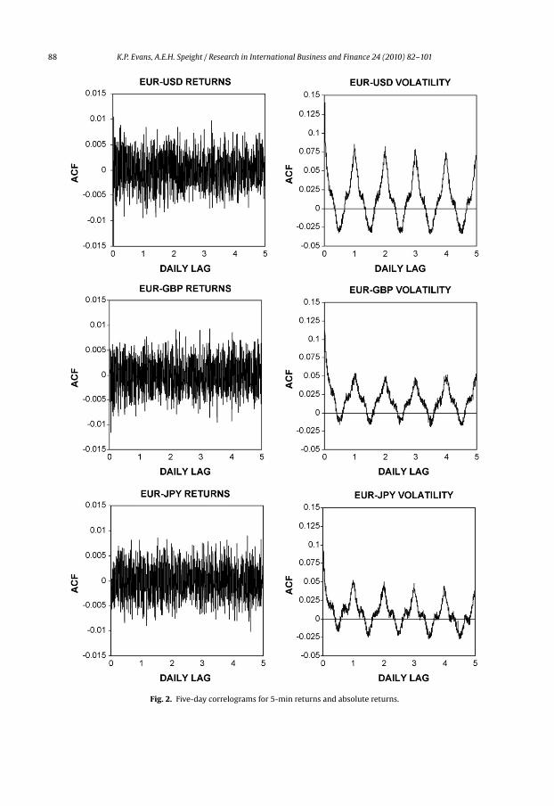
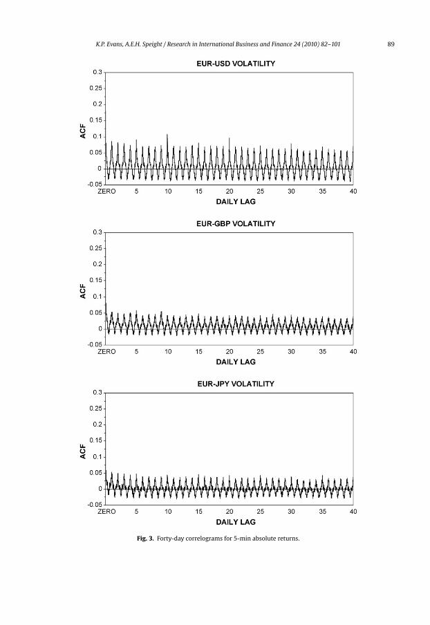
In order to characterise further the nature of intraday exchange rate periodicity, Fig. 2 shows plotsof the autocorrelation functions (ACFs) calculated to 1440 lags, corresponding to exactly five days,for 5-min returns and absolute 5-min returns.12 Consistent across the three exchange rates, ACFsfor returns shown in the left-hand column of Fig. 2, are economically small in magnitude and showno discernible pattern. ACFs for absolute returns, however, show a very distinctive U-shape patternoccupying precisely one day, which repeats continuously. This pattern is robust to the extension ofthe correlogram to a lag length of 40 days, as illustrated in Fig. 3. Each correlogram is dominatedby the daily periodic pattern, which causes a severe distortion to the long-run pattern. Abstractingfrom these patterns, however, reveals that the ACFs for absolute 5-min returns appear to decay veryrapidly initially, then extremely slowly thereafter. This confirms the findings of Andersen and Bollerslev(1997a,b, 1998), Bollerslev et al. (2000) and Andersen et al. (2000) that ACFs for high frequency absolutereturns tend to decay at a hyperbolic rate, indicating that they may represent fractionally integratedtime series processes displaying long memory characteristics.

Long memory processes have been demonstrated to describe the empirical properties of financialdata very well and are successful in modelling both the volatility of asset prices and power trans-formations of asset returns.13 As documented by Baillie (1996), the presence of long memory can bedefined in terms of the persistence of observed autocorrelations. Autocorrelations take far longer todecay than the exponential rate associated with ARMA models, persistence that is neither consistentwith an I(1) process nor an I(0) process. Formally, a particular process, yt, is said to be integrated oforder d, if (1 − L)dyt = ut, where L is a lag operator, −0.5 < d < 0.5, and ut is a stationary and ergodic pro-cess. For 0 < d < 0.5 the process is long memory and its autocorrelation function, �v at lag v, decays at ahyperbolic rate. Specifically, as v approaches infinity, �v = bv2d−1 where b is a factor of proportionality,v is the lag length of the ACF, d is the fractional integration parameter, and the implied hyperbolicdecay rate is v2d−1.

Time domain procedures for estimating the fractional integration parameter, d, are severely dis-torted by the presence of strong periodicity in the ACF for absolute returns and also require a strictlypositive correlogram, so that only after annihilating the daily dependencies does the long memoryfeature of high frequency returns data clearly stand out. Alternatively, in the presence of the distinctrepetitive pattern, semi-parametric, frequency domain procedures that explicitly ignore the intradayperiodicities are ideally suited to estimating d and the associated hyperbolic rate of decay. The log-periodogram regression estimator of Geweke and Porter-Hudak (GPH) (1983) has been utilised widelyin the literature. This estimator exploits the fact that if yt is a long memory process, the spectrum for

and end of the regular local business day, despite the possibility of around-the-clock foreign exchange trading and the absenceof complete market closure. More specifically, Hong and Wang (2000) suggest that traders in local markets have regular businesshours, towards the end of which they seek to achieve positions which they are content to hold overnight, and resume tradingwith the re-commencement of regular business hours the next day, adjusting their positions in light of information arrivalsduring non-business hours. Thus, trading in the Euro on Asian and European markets retains local components associated withregular business hours over the sample period. The same argument cannot, however, be applied to the heightened volatilityduring the overlap of trading in Europe and the US, with volatility during this period exhibiting an inverted U-shape.

12 For each currency, the first order ACF for returns are negative and statistically significant, but small in economic terms.Specifically they are −0.08, −0.19 and −0.11 for EUR–USD, EUR–GBP and EUR–JPY respectively. These are statistically significantwhen compared with the approximate 5% significance level of 0.01, which is not surprising given the large size of the sample.This is caused by foreign exchange traders positioning asymmetric quotes, relative to the perceived true market price, so as toattract a single trade on a very specific side of the price, which allows them to manage their inventory positions. As a result, themid-point of quoted prices tends to move in a fashion similar to that caused by bid-ask bounce. A large, negative first order ACFin returns generates a large positive ACF in absolute returns and these values are 0.18, 0.25 and 0.20 for EUR–USD, EUR–GBPand EUR–JPY respectively. These large first order ACFs are omitted from Fig. 2 for display purposes.

13 See Ding et al. (1993), Ding and Granger (1996), Granger and Ding (1996), Andersen and Bollerslev (1997a,b, 1998), Andersenet al. (2000), Bollerslev et al. (2000), and Bollerslev and Wright (2000). An excellent review of the early literature is providedby Baillie (1996).


Fig. 2. Five-day correlograms for 5-min returns and absolute returns.


Fig. 3. Forty-day correlograms for 5-min absolute returns.


Table 1Fractional integration parameter estimates.

GPH REISEN

EUR–USDd 0.2685 0.3041se 0.0357 0.0205t-stat1 −20.4635 −34.0019t-stat2 7.5117 14.8567t-stat3 −6.4759 −9.5726

EUR–GBPd 0.2244 0.2414se 0.0357 0.0205t-stat1 −21.6981 −37.0626t-stat2 6.2771 11.7959t-stat3 −7.7105 −12.6334

EUR–JPYd 0.3207 0.3321se 0.0357 0.0205t-stat1 −19.0027 −32.6345t-stat2 8.9725 16.2240t-stat3 −5.0151 −8.2053

the process should be linear for frequencies close to zero. Reisen (1994) offers an alternative semi-parametric frequency domain procedure for estimating d that uses a smoothed sample periodogram.Briefly stated, these estimators are obtained from the respective least squares regressions:

log[I( j)] = a0 + a1 log

[2 sin

( j2

)]2

+ ej, (1a)

log[fs( j)] = a0 + a1 log

[2 sin

( j2

)]2

+ uj, (1b)

where j = 2�j/n, j = 0, 1, 2, . . ., m, defines the set of harmonic frequencies, I( j) denotes the sampleperiodogram, f( j) and fs( j) denote the spectral density and smoothed periodogram of the pro-

cess, ej = log[I( j)/f( j)]−E log[I( j)/f( j)] and uj = log[fs( j)/f( j)] respectively, d = −(a1/2), and the

standard error of d is dependent only on m, according to√m(d− d)∼N(0,�2/24).14

Table 1 shows the two alternative estimates for the fractional integration parameter along withtheir standard errors for each of the absolute returns series, where t-stat1, t-stat2 and t-stat3 reporttest statistics for t tests under varying hypotheses. For t-stat1 the null hypothesis is that d = 1 and isrejected in all cases at the 1% level of significance in favour of the one-sided alternative hypothesisthat d < 1. For t-stat2 the null that d = 0 is also rejected in all cases at the 1% level in favour of the one-sided alternative that d > 0. Finally for t-stat3, the null hypothesis that d = 0.5 is rejected in all cases atthe 1% level in favour of the one-sided alternative that d < 0.5. Thus, the clear conclusion that can bedrawn from Table 1 is that d lies between 0 and 0.5 for the absolute returns of all three currency pairs,indicating that the three series are stationary, fractionally integrated and exhibit long memory.

3. Econometric method

As identified in Section 2, the volatility dynamics of high frequency foreign exchange returnsare characterised by pronounced intraday patterns, highly significant short-lived announcement

14 Further details of these, now commonly applied, estimators are omitted here in the interests of brevity. For a particularlylucid account, see Reisen (1994), and for discussion of the formal properties of these estimators see Robinson (1994a,b, 1995a,b)and Hurvich et al. (1998).


effects, and long memory properties. In the general modelling procedure adopted here, which followsAndersen and Bollerslev (1998), the volatility process is driven by the simultaneous interaction of thesecomponents associated with predictable calendar effects, macroeconomic news announcements and apotentially persistent, unobserved latent factor. The procedure allows standard regression techniquesto be used to simultaneously account for each separate component of volatility with the objectiveof isolating the dynamic behaviour of volatility around macroeconomic news announcements. In fullgenerality, the model takes the following form:

Rt,n − Rt,n = �t,n · st,n · Zt,n, (2)

where Rt,n is the expected 5-min return such thatRt,n − Rt,n measures excess returns, Zt,n is an indepen-dent and identically distributed zero mean, and unit variance error term, st,n represents the intradaypattern, calendar features and macroeconomic announcement effects, and �t,n denotes the remaininglatent, long memory, volatility component. All volatility components are assumed to be independentand non-negative. However, the components of Eq. (2) are not separately identifiable without addi-tional restrictions. Squaring and taking logs allow st,n to be isolated as the sole explanatory variable:

2 log[|Rt,n − Rt,n|] − log�2t,n = �0 + 2 log st,n + ut,n, (3)

where �0 = E[log Z2t,n] and ut,n = logZ2

t,n − E[log Z2t,n]. Since each particular macroeconomic news

announcement is unique, log st,n will be stochastic. The price and volatility reaction will reflect thenews content (the innovation relative to consensus forecasts) of the announcement, the dispersion ofbeliefs among traders and other market conditions at the time of the release. To capture these dynamicfeatures directly, it would be necessary to model a wide information set including expectations andrecent return innovations, for example, amongst other factors. To maintain simplicity at the outset,the (log) volatility response, conditional on the type of announcement, the time of release and otherrelevant calendar information, is merely assumed to have a well defined expected value, E[log st,n].This average impact is governed by purely deterministic regressors such that the innovation resultingfrom a new release, log st,n − E[log st,n] can be isolated. The final restriction is that log�t,n is strictlystationary and has a finite unconditional mean, E[log�t,n].

To obtain an operational regression equation, some additional structure is imposed. First, Rt,n isassumed constant and well approximated by the sample mean, R, which, as Andersen and Bollerslev(1998) explain, is an innocuous assumption given that the standard deviation dwarfs the mean return,implying that inferences are not sensitive to minor misspecification of the conditional mean. Second,to help control for systematic volatility movements caused by the latent volatility component, an apriori estimate of the return standard deviation, �t,n, is applied. Third, a parametric representationis imposed on the regressor E[log st,n] which accounts for calendar and announcement effects (seebelow). Since theory provides few guidelines regarding the precise shape of the intraday pattern,two adaptive functional forms, the FFF and cubic spline approaches, are chosen as alternatives. Abenefit to both of these approaches is that they use the entire span of data in fitting the intradaypattern, rather than relying on standardisation by the average intraday absolute, or squared, returnfor a particular interval.15 With the further introduction of announcement effect dummy variablesstructured by country of origin and window intervals surrounding the announcement timing, Ic,w(t, n),the operational regression then becomes:

2 log|Rt,n − R|�t,n

= �0 + E[log st,n] + �c,wIc,w(t, n) + ut,n, (4)

where the left-hand side variable measures logarithmic-squared, standardised absolute mean-adjusted returns, whilst the right-hand side variable E[log st,n] represents a choice of parametric

15 That is, it is also possible to remove the intraday volatility pattern in returns by standardizing absolute, mean-adjustedreturns by the mean absolute return for a particular interval, as plotted in Fig. 1 (see Andersen and Bollerslev, 1997a,b) or bythe mean squared return for a particular interval (Taylor and Xu, 1997). However, such techniques do not allow a sufficientlyaccurate separation of volatility spikes from the underlying intraday pattern for the investigation being conducted here, sincethe mean absolute return for an interval immediately following a macroeconomic announcement will be high and the veryeffect that is to be investigated is filtered away.


function that models the intraday volatility pattern and calendar features, while �0 = E[log Z2t,n] +

E[log�2t,n − log �2

t,n] and the error process ut,n is stationary. Two important empirical features of thisregression are that the use of mean-adjusted, 5-min returns annihilates the problem of returns witha value of zero and the log transformation eliminates any extreme outliers, rendering the regres-sion more robust. The potentially highly persistent volatility component, �t,n, in Eq. (4) is estimatedas follows. Daily volatility, �t, is estimated from GARCH models applied to a longer series of dailyreturns from 2nd January 1999 to 31st July 2003. Firstly, based on the temporal dependencies and longmemory properties evidenced in Section 3, a fractionally integrated MA(1)-FIGARCH(1,d,1) model isimplemented.16 This follows the approach of Bollerslev et al. (2000), and involves specifying a firstorder moving average process for the mean daily return, and conditional variance equation, givenrespectively by:

Rt = �0 + �1εt−1 + εt, (5a)

�2t = ω + ˇ�2

t−1 + [1 − ˇ1L − (1 − ϕL)(1 − L)d]ε2t , (5b)

where L represents the lag operator and d is the fractional integration parameter. Assuming that thislong-run volatility component is constant over the trading day, the associated intraday estimates are�t,n = �t/N1/2, where N = 288 represents the number of 5-min intervals during a trading day. Standard-isation of the mean-adjusted absolute returns by �t,n allows the volatility factor on the left-hand sideof (4) to vary over time thus improving the efficiency of the estimation, and is likely to eliminate thevolatility clustering and high persistence that is prevalent in financial data at the daily frequency. It isimportant to recognise, however, that this procedure may give rise to a generated regressors problemwhich may impart a bias to standard errors. To address this issue the time-varying estimates calcu-lated from Eq. (5b) are also compared to a constant daily volatility factor, which is free of any generatedregressor problem, calculated as �t,n = �/N1/2, where � denotes the sample mean of �t .

Finally, but importantly, the evidence in Fig. 1 suggests a violent reaction in volatility following someUS announcements, which persists for some time, and possibly the existence of elevated volatility in theintervals just prior to the announcement. To test explicitly for these dynamics, news announcementsare grouped by country with three indicator variables included in Eq. (4) for each country referenced byIc,w(t, n). This is a dummy variable relating to an announcement for country c occurring during intervaln on day t, wherew refers to an event window: a pre-announcement period (w = 1), a period just afterthe announcement (w = 2) and a post-announcement period (w = 3). The observation windows areequal to 15 min before the announcement (w = 1), 5 min just after the announcement (w = 2) and thefollowing 25 min after the announcement (w = 3).

4. Periodicity modelling

As noted in the introduction above, two alternative modelling techniques designed to capture intra-day pattern in volatility are compared.17 Firstly, following Andersen and Bollerslev (1998), Andersenet al. (2000) and Bollerslev et al. (2000), an adaptation of the FFF specification is defined as follows:

E[log st,n] = �1 +K∑k=1

�k · Ik(t, n) +Q∑q=1

(ıcos,q · cos

q2�Nn+ ısin,q · sin

q2�Nn). (6)

This expression is non-linear in the intraday time interval, n, parameterised by a number of sinusoidsthat occupy precisely one day and a set of calendar dummies, Ik, where Ik(t,n) is an indicator for calendarevent k occurring during interval n on day t. Q is a tuning parameter and refers to the order of expansion,while �k, ıcos,q and ısin,q are the fixed coefficients to be estimated. During periods of daylight saving

16 As a robustness check, a simple MA(1)-GARCH(1,1) model is also used for its simplicity and popularity, following the approachof Andersen and Bollerslev (1998).

17 There are, of course, further alternative methods available for estimating the intraday periodicity to use in this standardis-ation, for example Gencay et al. (2001) use a method based on a wavelet multi-scaling approach.


time the sinusoids are translated leftwards by 1 h using a time deformation procedure. Empirically,and consistent with results reported in Andersen and Bollerslev (1998), Q = 4 is selected based on thesignificance of estimated coefficients, the Akaike Information Criteria (AIC) and the success of themodel in fitting the intraday volatility pattern.

The second characterisation of the intraday volatility pattern uses a cubic spline specification,whereby, as recently advocated by Taylor (2004a,b), a series of third order polynomials are fittedbetween clearly defined ‘knots’ during the day:

E[log st,n] = �1 +K∑k=1

�k · Ik(t, n)

+M∑m=1

[˛1,mDm

(n− lmN

)+ ˛2,mDm

(n− lmN

)2

+ ˛3,mDm

(n− lmN

)3], (7)

where lm denotes the interval of the day in which knot m (m = 1, 2, . . ., M) is placed, and these arechosen a priori based on the underlying intraday pattern, Dm are dummy variables taking the value1 if n ≥ lm and 0 otherwise and ˛1,m, ˛2,m and ˛3,m are coefficients to be estimated. The knots are notchosen arbitrarily, but are chosen to reflect the geographical nature of the foreign exchange marketthat drives the distinctive intraday volatility pattern, and cubic splines are then fitted between theseknots.18 In addition to the flexibility of the positioning of the knots, an advantage of the cubic splinesover FFF is that it does not necessarily impose a smooth pattern on intraday volatility, but also allowssharp peaks and troughs. A clear example is the peak during morning trading in Europe and theUK. Whilst the intraday patterns are therefore very similar between the FFF and cubic splines, thecubic splines show far greater precision in modelling the volatility spikes around the knot positionsassociated with market opening and closing, and this may facilitate a clearer assessment of the impactof macroeconomic announcements coinciding with these knots, as well as other calendar effects.

The Ik(t,n) regressors in Eqs. (6) and (7) indicate dummy variables associated with holidays, week-days, and calendar related characteristics. Holiday dummies refer to regional holidays that causevolatility slowdowns but still provide reliable quotes and returns, and they only affect the portionof the trading day corresponding to the trading activity of the financial centre affected by the holidayand intervals during these holiday periods are assigned a value of unity (zero otherwise) to capturetheir effect explicitly. Similar simple dummy variables are also included for each day-of-the-week toaccount for any systematic weekly patterns in exchange rate volatility. A DST dummy is also includedto allow for systematically higher volatility during DST. The remaining calendar related characteristicsrefer to volatility jumps at the opening of markets in Tokyo and Hong Kong, Singapore and Malaysia,and volatility slowdowns surrounding weekends, especially during periods of DST. To account properlyfor these calendar effects whilst maintaining the cyclical periodicity of the intraday volatility pattern,a polynomial structure is imposed on the volatility response for these events. In full generality, if anevent affects volatility from time t0 to time t0 +˝, the impact on volatility can be represented overthe event window � = 0, 1, . . ., ˝ by a polynomial specification: p(�) = c0 + c1� + ··· + cp�p. As arguedby Andersen et al. (2003), the use of lower ordered polynomials constrains the volatility response inhelpful ways: by promoting parsimony, by retaining flexibility of approximation and by facilitatingthe imposition of sensible constraints on the response pattern. Specifically, enforcing p(0) = 0 ensuresthere is no jump in volatility away from the underlying intraday pattern and p(˝) = 0 enforces the

18 In light of the 24 h intraday volatility pattern, there are five knots imposed in total (M = 5). The first knot is positioned atinterval 0 (21:00 GMT), l1 = 0, corresponding to the start of the trading day in Sydney, and l2 = 36 (00:00 GMT) such that thesecond knot corresponds to the opening of markets in Tokyo. A further knot is positioned at l3 = 96 (5:00GMT) in winter tocapture the volatility slowdown before the onset of early trading in Europe and this is shifted leftwards by one hour duringdaylight saving time (DST) in summer (l3 = 84 corresponding to 4:00 GMT). Similarly, l4 = 132 during winter and l4 = 120 duringDST (8:00 and 7:00 GMT, respectively) to position the fourth knot at the volatility peak occurring at the overlap of the close oftrading in Japan and the opening of trading in Europe and the UK, and finally, l5 = 216 in winter and 204 in DST (15:00 and 14:00GMT) at the highest point of the intraday pattern.


requirement that the impact effect slowly fades to zero. The latter constraint gives rise to a polynomialwith one less parameter:

p(�) = c0[

1 −(�

˝

)P]+ · · · + c1�

[1 −

(�

˝

)P−1]

+ cP−1�P−1

[1 − �

˝

]. (8)

Based on close inspection of the data underlying the intraday patterns presented in Fig. 1, the Tokyoopening effect is afforded a linear response (P = 1) beginning at 00:05 GMT and lasting until 00:30GMT (˝= 6) with the effect fading to zero at 00:35 GMT (p(˝) = 0). Identical structure applies to thesimultaneous opening of Hong Kong, Singapore and Malaysia but the effect begins 1 h later at 01:05GMT. To account for a Monday morning slowdown, when traders in Sydney and Wellington are theonly participants active in the market, a second order polynomial (P = 2) is imposed from 21:05 GMTto 23:00 GMT (˝= 23) with the restriction that p(˝) = 0 ensuring the effect fades to zero. Similarly,a Friday night slowdown, when US traders are the only active group, is also modelled by a secondorder polynomial. This effect begins at 17:05 GMT in winter time and lasts until 21:00 GMT (˝= 47),with the start of the effect shifted by 1 h to 16:05 GMT (˝= 59) during DST. For this polynomial therestriction that p(0) = 0 ensures that there is no step away from the intraday pattern at the impact ofthe event. The leftward shift of the intraday pattern by 1 h during DST gives rise to a hiatus betweenclose of trading in the US and the opening of trading in Wellington and this is accommodated by asecond order polynomial for each day during DST beginning at 19:05 GMT and lasting until 21:00GMT (˝= 23) with the restrictions p(˝) = 0 and p(0) = 0 imposed. The last calendar effect is a winterslowdown which occurs for EUR–USD only, whereby volatility tends to be lower in the early part ofthe trading day and this effect is accounted for by a second order polynomial beginning at 21:05 GMTon days during winter time and lasting until 00:00 GMT (J = 35). The effect of the winter slowdownpolynomial is restricted to reach zero at 00:00 GMT (p(˝) = 0).

5. Empirical results

Before turning to discussion of the effects of macroeconomic announcement effects by country onEuro exchange rate volatility, the results of the modelling procedures for intraday periodicity and cal-endar effects are first presented.19 Table 2 shows the estimated coefficients and their robust t statisticsfor the coefficients of the alternative means of capturing the intraday volatility pattern given by theFFF and cubic spline function methods represented by Eqs. (6) and (7) in conjunction with Eq. (4).20

Table 3 reports the �k coefficient estimates and their associated robust t statistics for the calendareffects. There is a strong market opening effect in Tokyo and the effect appears to be stronger underthe FFF specification. This is entirely expected since the flexibility of the cubic spline formulation allowsthe positioning of a knot at 00:00 GMT, precisely the same time as the onset of this calendar event,allowing some of the Tokyo market opening effect to be captured by the intraday pattern. That is, theFFF pattern is more cyclical in design and so a more aggressive jump in volatility away from this FFFpattern occurs at Tokyo market opening. The effect is also stronger for EUR–JPY, with the opening of

19 All of the model coefficients are estimated simultaneously, but they are presented separately to ease clarity of tabulationand interpretation. Whilst not presented here in full, the results of an alternative version of the model in which absolute mean-adjusted returns are standardised using the sample mean of �t,n , and thus ignores any temporal variation in this volatility factor,have also been considered. Whilst this version of the model does nothing to alleviate heteroscedasticity at the daily frequency,it ensures that there is no practical generated regressors problem, which may exist when using �t,n . The parameter estimatesare largely unchanged and the qualitative features of the inference unaffected, so the use of �t,n does not, therefore, seem to giverise to a generated regressors problem. As a further robustness check, estimation results for both these versions of the modelthat uses �t,n as the daily volatility factor generated from an orthodox MA(1)-GARCH(1,1) model, rather than its fractionallyintegrated counterpart, have also been considered. Again, parameter estimates and inferences are similar to those discussedin the text, and confirm that the intraday pattern and calendar features described in the text are not unduly influenced by thechoice of the daily volatility measure.

20 Although not shown here to conserve space, plots of the sample average log volatility patterns superimposed on the fittedintraday volatility patterns, and ACFs of the filtered returns and absolute returns series, both serve as an additional diagnostictest of the performance of the intraday periodicity filters in modelling the intraday volatility pattern. These plots reveal thatboth the FFF and cubic spline specifications perform very well in this regard and for EUR–USD and EUR–JPY in particular.


Table 2Estimated intraday periodicity models.

FFF Cubic spline

Coefficient EUR–USD EUR–GBP EUR–JPY Coefficient EUR–USD EUR–GBP EUR–JPY

�0 +�1 −2.478 −2.279 −2.379 �0 +�1 −3.023 −2.844 −2.917(−50.05) (−42.06) (−44.81) (−17.22) (−14.00) (−16.97)

ıcos,1 −0.252 −0.209 −0.197 ˛1,1 8.010 13.777 11.663(9.13) (−6.79) (−6.601) (0.85) (1.16) (1.19)

ıcos,2 −0.110 0.063 −0.056 ˛2,1 −321.32 −224.23 −287.58(−4.16) (2.11) (−1.96) (−1.98) (−1.10) (−1.68)

ıcos,3 −0.277 −0.269 −0.284 ˛3,1 2234.3 1029.3 1896.5(−11.08) (−9.41) (−10.39) (2.78) (1.04) (2.24)

ıcos,4 0.123 0.041 0.044 ˛1,2 −37.019 −12.369 −35.391(5.18) (1.49) (1.69) (−4.61) (−1.34) (−4.37)

ısin,1 −0.614 −0.648 −0.434 ˛2,2 −505.88 −142.43 −408.60(−23.89) (−22.33) (−15.57) (−3.51) (−0.82) (−2.71)

ısin,2 −0.140 −0.007 0.012 ˛3,2 −2240.5 −1042.6 −1906.7(−5.58) (−0.24) (0.45) (−2.78) (−1.05) (−2.25)

ısin,3 0.154 0.172 0.109 ˛1,3 5.713 4.179 −0.645(6.26) (6.26) (4.09) (0.96) (0.58) (−0.10)

ısin,4 −0.112 −0.052 −0.096 ˛2,3 84.729 155.71 246.09(−4.73) (−1.94) (−3.76) (0.75) (1.13) (1.96)

˛3,3 −211.21 −676.97 −1204.9(−0.35) (−0.92) (−1.78)

˛1,4 −29.874 −21.472 −9.970(−3.66) (−2.30) (−1.08)

˛2,4 47.904 132.42 226.35(0.42) (0.98) (1.77)

˛3,4 174.43 645.74 1197.2(0.28) (0.86) (1.73)

˛1,5 −10.170 1.164 −0.292(−2.17) (0.23) (−0.06)

˛2,5 −84.505 −97.671 −92.915(−3.20) (−3.31) (−3.30)

˛3,5 188.41 261.63 208.41(2.29) (2.85) (2.37)

Notes: The table reports the estimated coefficients and their Newey and West (1987) robust t statistics shown in parentheses forEq. (4), using Eqs. (6) and (7) as alternative specifications for the intraday volatility pattern. More specifically, the table reports asub-set of the coefficient estimates for the intraday periodicity models alone (calendar effect estimates suppressed, see Table 3;macroeconomic announcement effect estimates suppressed, see Table 4). Returns are calculated from 5-min logarithmic averagebid-ask quotes from 2nd January 2002 to 31st July 2003. Quotes from Friday 21:05 to Sunday 21:00 are excluded giving 118,656observations. The absolute value of mean-adjusted 5-min returns is standardised by a daily volatility factor obtained from aMA(1)-FIGARCH(1,d,1) model fitted to a longer daily sample of spot exchange rates from 2nd January 1999 to 31st July 2003 asspecified by Eq. (5). Bold denotes significant coefficients at a minimum 5% level of significance.

markets in Tokyo causing higher volatility for JPY. There is also a noticeable increase in volatility, andfor EUR–JPY in particular, caused by the simultaneous opening of markets in Hong Kong, Singaporeand Malaysia. Since there is no knot positioned at 1:00 GMT in the cubic spline pattern, the coefficientestimates for this effect are very similar for both intraday model specifications.

EUR–USD volatility decreases considerably during regional holidays, as expected, and this effect isalso apparent for EUR–GBP and EUR–JPY although it is not statistically significant in these latter cases.In contrast, Monday morning and Friday evening slowdowns are not significantly different from zerofor any currency. However, there is clear evidence of a slowdown in EUR–USD volatility in the earlypart of days during winter time. The shift in timing regimes from winter to DST causes a leftward shiftin the intraday pattern by 1 h, but this generates a significant slowdown in volatility at the end of theday for EUR–USD only, and is specific to the FFF intraday pattern. Volatility is systematically higherduring DST and statistically significantly so in five of the six models estimated. Finally, there is a strongday-of-the-week effect with Tuesdays and Thursdays showing particularly high volatility relative tothe other weekdays.


Table 3Calendar effects.

FFF Cubic spline

Coefficient EUR–USD EUR–GBP EUR–JPY Coefficients EUR–USD EUR–GBP EUR–JPY

Tokyo 0.487 0.550 0.633 Tokyo 0.168 0.454 0.389(3.90) (3.43) (4.83) (1.24) (2.58) (2.77)

Hong Kong 0.230 0.233 0.430 Hong Kong 0.227 0.286 0.457(1.98) (1.57) (3.64) (2.02) (1.97) (4.02)

Holiday −0.258 −0.034 −0.097 Holiday −0.258 −0.028 −0.093(−4.02) (−0.46) (−1.40) (−4.03) (−0.37) (−1.34)

Monday −0.203 0.099 −0.284 Monday −0.317 0.179 −0.371Early (−0.83) (0.39) (−1.09) Early (−1.25) (0.62) (−1.30)

0.035 0.059 −0.007 0.039 0.030 −0.006(0.77) (1.30) (−0.16) (0.80) (0.57) (−0.11)

Friday −0.011 −0.001 −0.011 Friday −0.010 0.001 −0.008Late (−0.91) (−0.09) (−0.89) Late (−0.79) (0.06) (−0.59)

0.000 0.000 0.000 0.000 0.000 0.000(0.90) (0.56) (1.33) (0.82) (0.42) (0.98)

Winter −0.444 Winter −0.549Slowdown (−2.45) Slowdown (−2.58)

0.023 0.035(1.05) (1.43)

Summer −0.047 −0.018 −0.001 Summer −0.035 −0.017 −0.015Slowdown (−2.50) (−0.79) (−0.03) Slowdown (−1.58) (−0.64) (−0.65)Summer 0.202 0.131 0.104 Summer 0.217 0.146 0.070

(5.55) (3.33) (2.70) (3.14) (2.13) (1.08)Tuesday 0.350 0.304 0.330 Tuesday 0.347 0.302 0.327

(6.35) (4.97) (5.60) (6.30) (4.94) (5.54)Wednesday 0.163 0.087 0.119 Wednesday 0.160 0.084 0.116

(2.49) (1.21) (1.66) (2.44) (1.18) (1.62)Thursday 0.378 0.343 0.376 Thursday 0.379 0.343 0.374

(6.83) (5.61) (6.38) (6.86) (5.61) (6.33)Friday 0.141 0.107 0.134 Friday 0.138 0.102 0.134

(2.04) (1.43) (1.81) (1.99) (1.36) (1.74)

Notes: The table reports the estimated coefficients and their Newey and West (1987) robust t statistics shown in parenthesesfor Eq. (4) in conjunction with Eqs. (6) and (7) as alternative specifications for the intraday volatility pattern. More specifically,the table reports coefficient estimates for the calendar effect variables, �k (intraday periodicity model estimates suppressed,see Table 2; macroeconomic announcement effect estimates suppressed, see Table 4). For further details of sample period anddaily volatility factor model, see notes to Table 2. Bold denotes significant coefficients at a minimum 5% level of significance.

Furthermore, it is possible to consider the economic significance of the estimated coefficients relat-ing to the calendar effects in Table 3. The �k estimators associated with the simple dummy variablesmeasure an incremental, multiplicative factor to volatility. A coefficient of unity signifies a multiplica-tive factor of exp(1/2) ≈ 1.65, thus volatility increases by an incremental 65% in the correspondinginterval. For the FFF intraday volatility model for example, EUR–USD volatility for intervals duringregional holidays is 12.10% lower than usual, with the effect applied uniformly to each interval coveredby the holiday dummy. There is an incremental increase in volatility per interval of 10.63% during DST,19.13% on Tuesdays, 8.49% on Wednesdays, 20.80% on Thursdays and 7.30% on Fridays. The correspond-ing figures for EUR–GBP and EUR–JPY are much smaller and all of these effects are confirmed by theremarkably similar estimates obtained form the cubic spline intraday volatility model.

Interpretation of the other calendar effects is more complex because the regressors are notsimple dummy variables, but involve dynamic response patterns governed by polynomial struc-tures. The instantaneous jump in volatility is then calculated as exp(p(0)/2)−1, the response at the�th lag equals exp(p(�)/2)−1, and the cumulative response over the response horizon is given by∑

�=0,˝[exp(p(�)/2) − 1]. The Tokyo market opening for the FFF intraday model, for example, showsan instantaneous jump measure of 0.276 and a cumulative response measure of 0.932, which implythat volatility jumps by 27.57% in the interval immediately following the opening of markets in Tokyoand that a proportion 0.932 of the average absolute return during this period is added over the event’s


response horizon. Since volatility is low at this time of day at 0.02%, the full impact over the eventhorizon amounts to an additional 0.0186%.

The median daily cumulative absolute return for EUR–USD over the sample is 7.42%, so the Tokyoopening effect constitutes only 0.138% of the return variability over a typical trading day. Therefore,although the effect is statistically significant, it is of limited economic importance. Unsurprisingly,the Tokyo opening effect is larger for EUR–JPY and the corresponding estimates for EUR–JPY show aninstantaneous jump in volatility of 37.23%, but a cumulative response of only 0.188% of the mediandaily cumulative absolute return (which is 7.55% for EUR–JPY). The effect on EUR–GBP is smaller thanEUR–JPY, but larger than EUR–USD. The coefficient estimates for this effect are lower for each currencywhen using the cubic spline version of the intraday volatility because of the position of a knot at Tokyomarket opening. The opening of markets in other East Asian centres produces lower coefficient esti-mates for the FFF model than the Tokyo market opening effect, showing that this event contributesan even smaller proportion to daily return variability, with very similar estimates obtained under thecubic spline specification. Even the largest coefficient associated with the ‘Hong Kong’ effect, shownfor the cubic spline version for EUR–JPY, explains only 0.131% of the daily EUR–JPY returns variability.21

Therefore, although these calendar effects present interesting deviations from the intraday volatilitypattern, in many cases they are only marginally statistically significant and are insignificant in eco-nomic terms, as judged by their effect on volatility over the entire horizon of the response and againstcumulative absolute returns over a typical day.

Finally, but perhaps most importantly, the estimates of the �c,w coefficients reported in Table 4measure the volatility response during the three event windows with a total of three coefficientsestimated for each of the six points of origin of major macroeconomic news releases. In general, theevidence in Table 4 shows that the predominant reaction of volatility, across all three exchange rates,occurs in response to US macroeconomic news, with the majority of the increase in volatility occurringafter the announcement, as shown by the statistical significance of coefficients for event windowsw = 2 and w = 3. This confirms the previous empirical findings of Andersen and Bollerslev (1998)and Andersen et al. (2003), but the broader range of macroeconomic announcements internationallythat are considered here also reveals that on average, Eurozone, German and UK announcements alsocause significant increases in exchange rate volatility, whilst French and Japanese macroeconomicannouncements mostly fail to exert any significant influence on EUR exchange rates.

More specifically, US announcements cause significant and sizeable responses in volatility forall three exchange rates for event windows w = 2 and w = 3, suggesting that such announcementscause immediate pronounced increases in volatility of up to 89.46%, 47.80% and 47.18% for EUR–USD,EUR–GBP and EUR–JPY respectively, which persist for some time after the announcement, raisingvolatility by up to 23.01%, 16.42% and 13.66% on average in each of the five intervals following theinstantaneous response. In contrast to the findings of Bauwens et al. (2005), US news does not causea volatility reaction prior to scheduled announcement times. Eurozone announcements also causesignificant increases in volatility in the announcement window (w = 2), the magnitude of which aresimilar across all three exchange rates. Eurozone announcements also cause significant increases involatility in the 15-min pre-announcement window (w = 1), consistent with the results of Bauwenset al. (2005), for EUR–USD and EUR–GBP, but not EUR–JPY. This effect is most likely caused by a sin-gle Eurozone announcement, namely interest rate decisions by the ECB. Possible explanations forthis pre-announcement reaction include information leakage in the minutes prior to the announce-ment, or slight departures from scheduled release times. Alternatively, and as suggested by Bauwenset al. (2005), it is possible that ECB announcements attract traders who wish to make anticipatorytrades based on their personal beliefs, or who wish to minimise their exposure prior to interest rateannouncements being made.22 However, although these coefficients are statistically greater than zero,they are far smaller than the corresponding effects for US news, with the Eurozone announcements

21 The analysis of the other statistically significant calendar effects reveals a similar conclusion. The early volatility slowdownduring winter time for EUR–USD and the summer slowdown reduce volatility by only 0.408% and 0.291% of the median dailycumulative absolute returns, at most.

22 The significant rise in volatility in the post-announcement window following Eurozone news announcements is consistentwith previous evidence reported by Perez-Quiros and Sicilia (2002), which suggests that financial markets have predicted the


Table 4Volatility dynamics surrounding announcements.

Coefficient FFF Cubic spline

EUR–USD EUR–GBP EUR–JPY EUR–USD EUR–GBP EUR–JPY

�US,1 0.0784 0.0902 0.1179 −0.0223 0.0154 0.0508(0.9284) (0.8532) (1.2991) (−0.2748) (0.1484) (0.5805)

�US,2 1.2736 0.7734 0.7588 1.2780 0.7814 0.7729(9.6794) (4.8669) (5.7520) (9.7442) (4.9180) (5.8952)

�US,3 0.4142 0.3041 0.2443 0.3151 0.2566 0.2560(5.2814) (3.4723) (3.1083) (4.3117) (3.0262) (3.4614)

�EU,1 0.3366 0.3899 0.1138 0.2799 0.3139 0.0661(2.8362) (2.8101) (0.9372) (2.4339) (2.1912) (0.5512)

�EU,2 0.3463 0.3855 0.3992 0.3685 0.4388 0.4074(1.7821) (1.6673) (2.0029) (1.8975) (1.9104) (2.0430)

�EU,3 0.2210 0.3599 0.1777 0.1551 0.3087 0.1553(2.0918) (2.9745) (1.6765) (1.5266) (2.6497) (1.4267)

�GER,1 −0.0311 −0.1732 −0.1048 −0.0492 −0.1926 −0.1243(−0.2683) (−1.2844) (−0.8712) (−0.4296) (−1.3661) (−1.0348)

�GER,2 0.3498 0.2126 0.0897 0.3789 0.1878 0.0887(2.0311) (0.9990) (0.4421) (2.1856) (0.8751) (0.4380)

�GER,3 0.2263 0.1863 0.0725 0.2196 0.1574 0.1308(2.7395) (1.7847) (0.7747) (2.6388) (1.4800) (1.4594)

�FRA,1 0.1810 0.1800 0.0976 0.0661 0.0800 −0.0043(1.5618) (1.3578) (0.7863) (0.5787) (0.6125) (−0.0366)

�FRA,2 0.0850 0.0628 0.0438 −0.1007 −0.1268 −0.0631(0.4194) (0.2438) (0.2268) (−0.4862) (−0.4859) (−0.3164)

�FRA,3 0.0660 −0.0187 0.0801 0.0439 −0.1005 0.0468(0.7171) (−0.1584) (0.7348) (0.4293) (−0.7847) (0.4023)

�UK,1 −0.0628 −0.2270 −0.0072 −0.0221 −0.2018 −0.0093(−0.5902) (−1.4633) (−0.0581) (−0.2097) (−1.3179) (−0.0753)

�UK,2 0.0847 0.7870 −0.2310 0.1754 0.8657 −0.1682(0.4698) (3.2920) (−1.1177) (0.9738) (3.6235) (−0.8143)

�UK,3 0.2182 0.1485 0.1808 0.1912 0.1956 0.1975(2.1780) (1.2636) (1.7812) (1.9772) (1.7170) (1.9367)

�JAP,1 0.0473 0.2575 −0.1317 0.0006 0.2780 −0.1092(0.3733) (1.5831) (−0.8931) (0.0045) (1.6769) (−0.7629)

�JAP,2 0.0488 −0.1029 0.1211 −0.0109 −0.0737 0.0890(0.2607) (−0.3814) (0.5993) (−0.0582) (−0.2718) (0.4372)

�JAP,3 0.0830 −0.1726 0.0219 0.1403 0.0418 0.0182(0.7437) (−1.2056) (0.1752) (1.2739) (0.3105) (0.1536)

Notes: The table shows coefficient estimates and their associated Newey and West (1987) robust t statistics in parenthesesobtained from the estimation of Eq. (4) using Eqs. (6) and (7) as alternative specifications for the intraday volatility pattern.More specifically, the table reports coefficient estimates for the news announcement indicator variables, �c,w , for each country(c) and event window (w) (intraday periodicity model estimates suppressed, see Table 2; calendar effect estimates suppressed,see Table 3). The event windows are 15 min prior to an announcement (w = 1), 5 min immediately after an announcement(w = 2) and the following 25 min after the announcement (w = 3). For further details of sample period and daily volatility factormodel, see notes to Table 2. Bold denotes significantly positive coefficients at a minimum 5% level of coefficient significance.

increasing volatility by up to 21.52% and 24.53% in the pre-announcement and announcement periodsrespectively.

Concerning other European announcement effects, German macroeconomic news has a significantcontemporaneous, w = 2, and post-announcement effect, w = 3, on EUR–USD volatility, confirmingand extending previous results for the intraday DEM–USD exchange rate reported by Chang and Taylor(2003). UK macroeconomic announcements have a significant contemporaneous effect on EUR–GBP

monetary policy decisions of the ECB rather well, though not perfectly. The important role of ECB announcements during thepre-announcement window is also consistent with the evidence reported recently by Sager and Taylor (2004), which suggeststhat ECB Governing Council decisions contain significant news content and that, whilst there is some evidence of position takingin the hour prior to ECB announcements, this may reflect dealers closing out positions in order to minimise their risk exposureprior to the announcement, rather than indicating information leakage.


volatility during event windoww = 2, but a more delayed impact on EUR–USD and EUR–JPY volatilityduring event windoww = 3. Macroeconomic announcements from France have no statistically signif-icant effects on volatility for any of the three exchange rates considered and Japanese macroeconomicnews increases EUR–GBP volatility in the pre-announcement window for the cubic spline specificationonly.

In terms of the robustness of the results to the intraday periodicity filters applied, the resultsreported are broadly invariant to the filter adopted. However, there are some notable differences inthe results between the FFF and cubic spline intraday periodicity models. Volatility reactions dur-ing the announcement window (w = 2) tend to be larger under the cubic spline specification, whilstthe responses during the post-announcement window tend to be higher for the FFF intraday model,and this is particularly evident for US, Eurozone, German and UK news. Since many US and Eurozoneannouncements coincide with the positioning of knots in the cubic spline intraday pattern, this findingsuggest that the cubic splines show greater precision than the FFF in modelling volatility peaks aroundboth market opening and, more importantly, around spikes associated with the release of macroeco-nomic information. The cubic spline model results therefore imply that announcement effects causelarger instantaneous Euro volatility and are far more quickly absorbed into exchange rates than is sug-gested by the FFF model results, and underscores the advantage of the flexible knot positioning in thecubic spline case, which permits the intraday periodicity to be more closely identified.

6. Conclusions

The components of high frequency returns volatility are not only significant and interesting in sta-tistical and economic terms, but the identification and accurate modelling of their dynamics is alsoa crucial precursor to their formal econometric modelling using models of the GARCH or stochasticvolatility varieties, and for the analysis of macroeconomic announcement effects on foreign exchangemarket volatility. Using a 19-month sample of 5-min returns for Euro–Dollar, Euro–Sterling andEuro–Yen exchange rates, and therefore a new market setting, this study confirms a 24 h pattern forintraday volatility, with volatility rising at the opening and overlapping of trading activity in the world’smajor financial centres. Whilst previous studies of this type commonly filter intraday volatility by fit-ting a Fourier flexible form (FFF) to the intraday pattern, this study compares the performance of theFFF with an alternative cubic spline approach. A particular advantage of the cubic spline method overthe FFF approach is that it does not impose a smooth pattern on intraday volatility, but allows sharppeaks and troughs. Consequently, the cubic spline method is able to provide a closer characterisationof the changing nature of periodicity through the 24 h foreign exchange trading cycle, and the sharpchanges in volatility associated with market opening and closing times. A clear example is providedby the peak in volatility during morning trading in Europe and the UK. The superiority of the cubicspline approach in this regard is also confirmed by, for example, the absence of significant timingeffects associated with the opening of trading exchanges in Tokyo under the cubic spline method butnot under the FFF approach.

Further analysis of various potential calendar effects associated with seasonal chronologicalchanges reveals that these calendar effects present interesting deviations from the average intradayvolatility pattern, with notable volatility increases associated with the change to daylight saving time,Tuesdays and Thursdays. However, such intraday timing effects are in many cases only marginally sta-tistically significant and are insignificant in economic terms, as judged by their effect on volatility overthe entire horizon of the response and against cumulative absolute returns measured over a typical day.Concerning the robustness of our findings to the two alternative intraday periodicity filters employed,the cubic spline model results imply that announcement effects are larger immediately followingthe announcement and are far more quickly absorbed into exchange rates in the post-announcementperiod than is suggested by the FFF model results, which underscores the advantage of the flexibilityof the cubic spline approach in permitting intraday volatility periodicity to be more closely identified.

Finally, examination of the exchange rate volatility response to macroeconomic announcementsemanating from the US, Eurozone, UK, France, Germany and Japan reveals that the predominant reac-tion of volatility, across all three exchange rates, occurs in response to US macroeconomic news,but also reveals that, on average, Eurozone, German and UK announcements also cause significant


reaction in exchange rate volatility. Whilst the majority of such reactions in volatility occur after theannouncement, Eurozone announcements are found to impact significantly upon volatility in the pre-announcement period. Possible explanations for this finding, which might usefully be addressed infuture research, include information leakage in the period leading up to the announcement, departuresfrom scheduled release times, or positioning by traders in the run-up to ECB interest rate announce-ments.

References

Abhyankar, A., Copeland, L.S., Wong, W., 1999. LIFFE cycles: intraday evidence from the FTSE 100 stock index futures market.Eur. J. Finance 5, 123–139.

Andersen, T.G., Bollerslev, T., 1997a. Intraday periodicity and volatility persistence in financial markets. J. Empirical Finance 4,115–158.

Andersen, T.G., Bollerslev, T., 1997b. Heterogeneous information arrivals and return volatility dynamics: uncovering the long-runin high frequency returns. J. Finance 52, 975–1005.

Andersen, T.G., Bollerslev, T., 1998. Deutsche mark-dollar volatility: intraday activity patterns, macroeconomic announcements,and longer run dependencies. J. Finance 53, 219–265.

Andersen, T.G., Bollerslev, T., Cai, J., 2000. Intraday and interday volatility in the Japanese stock market. J. Int. Financial MarketsInst. Money 10, 107–130.

Andersen, T.G., Bollerslev, T., Diebold, F.X., Vega, C., 2003. Micro effects of macro announcements: real-time price discovery inforeign exchange. Am. Econ. Rev. 93, 38–62.

Baillie, R.T., 1996. Long memory processes and fractional integration in econometrics. J. Economet. 73, 5–59.Baillie, R.T., Bollerslev, T., 1990. Intraday and inter-market volatility in foreign exchange rates. Rev. Econ. Stud. 58, 565–585.Ballocchi, G., Dacorogna, M.M., Hopman, C.M., Müller, U.A., Olsen, R.B., 1999. The intraday multivariate structure of the Eurofu-

tures markets. J. Empirical Finance 6, 479–513.Bauwens, L., Omrane, W.B., Giot, P., 2005. News announcements, market activity and volatility in the euro/dollar foreign exchange

market. J. Int. Money Finance 24, 1108–1125.Bollerslev, T., Cai, J., Song, F.M., 2000. Intraday periodicity, long memory volatility, and macroeconomic announcement effects

in the U.S. Treasury bond market. J. Empirical Finance 7, 37–55.Bollerslev, T., Domowitz, I., 1993. Trading patterns and prices in the interbank foreign exchange market. J. Finance 48, 1421–1443.Bollerslev, T., Wright, J.H., 2000. Semiparametric estimation of long-memory volatility dependencies: the role of high-frequency

data. J. Econ. 98, 81–106.Cai, C.X., Hudson, R., Keasey, K., 2004. Intraday bid-ask spreads, trading volume and volatility: recent empirical evidence from

the London Stock Exchange. J. Bus. Finance Accoun 31, 647–676.Chang, Y., Taylor, S.J., 2003. Information arrivals and intraday exchange rate volatility. J. Int. Financial Markets Inst. Money 13,

85–112.Cyree, K.B., Griffiths, M.D., Winters, D.B., 2004. An empirical examination of the intraday volatility in euro–dollar rates. Quart.

Rev. Econ. Finance 44, 44–57.Dacorogna, M.M., Müller, U.A., Nagler, R.J., Olsen, R.B., Pictet, O.V., 1993. A geographical model for the daily and weekly seasonal

volatility in the foreign exchange market. J. Int. Money Finance 12, 413–438.Daigler, R.T., 1997. Intraday futures volatility and theories of market behaviour. J. Futures Markets 17, 45–74.Ding, Z.X., Granger, C.W.J., 1996. Modeling volatility properties of speculative returns: a new approach. J. Economet. 73, 185–215.Ding, Z.X., Granger, C.W.J., Engle, R.F., 1993. Long memory properties of stock market returns and a new model. J. Empirical

Finance 1, 83–106.Ekman, P.D., 1992. Intraday patterns in the S&P 500 index futures market. J. Futures Markets 12, 365–381.Engle, R., Russell, J., 1998. Autoregressive conditional duration: a new model for irregularly spaced transaction data. Econometrica

66, 1127–1162.Gencay, R., Selcuk, F., Whitcher, B., 2001. Differentiating intraday seasonalities through wavelet multi-scaling. Physica A 289,

543–556.Geweke, J., Porter-Hudak, S., 1983. The estimation and application of long memory time series models. J. Time Series Anal. 4,

221–238.Giot, P., 2005. Market risk models for intraday data. Eur. J. Finance 11, 309–324.Granger, C.W.J., Ding, Z.X., 1996. Varieties of long memory models. J. Economet. 73, 61–77.Harris, L., 1986. A transactions data study of weekly and intradaily patterns in stock returns. J. Financial Econ. 16, 99–117.Hong, H., Wang, J., 2000. Trading and returns under periodic market closures. J. Finance 55, 297–354.Hurvich, C.M., Deo, R., Brodsky, J., 1998. The mean square error of Geweke and Porter-Hudak’s estimtes of the memory parameter

of a long-memory time series. J. Time Series Anal. 15, 285–302.Kawaller, I.G., Koch, P.D., Peterson, J.E., 1994. Assessing the intraday relationship between implied and historical volatility. J.

Futures Markets 14, 323–346.Kawaller, I.G., Koch, P.D., Koch, T.W., 1990. Intraday relationships between volatility in S&P 500 futures prices and volatility in

the S&P 500 index. J. Banking Finance 14, 373–397.Lee, J.H., Linn, S.C., 1994. Intraday and overnight volatility of stock index and stock index futures returns. Rev. Futures Markets

13, 1–30.Lockwood, L.J., Linn, S.C., 1990. An examination of stock market return volatility during overnight and intraday periods,

1964–1989. J. Finance 45, 591–601.McInish, T.H., Wood, R.A., 1990. A transactions data analysis of the variability of common stock returns during 1980–1984. J.

Banking Finance 14, 99–112.


Müller, U.A., Dacorogna, M.M., Olsen, R.B., Pictet, O.V., Schwarz, M., Morgenegg, C., 1990. Statistical study of foreign exchangerates, empirical evidence of a price change scaling law, and intraday analysis. J. Banking Finance 14, 1189–1208.

Newey, W.K., West, K.D., 1987. A simple, positive semi-definite, heteroskedasticity and autocorrelation consistent covariancematrix. Econometrica 55, 703–708.

Perez-Quiros, G., Sicilia, J., 2002. Is the European Central Bank (and the United States Federal Reserve) predictable? ECB WorkingPaper No. 192.

Reisen, V.A., 1994. Estimation of the fractional difference parameter in the ARFIMA (p,d,q) model using the smoothed peri-odogram. J. Time Series Anal. 15, 335–351.

Robinson, P.M., 1994a. Time series with strong dependence. In: Sims, C.A. (Ed.), Proceedings of the Sixth World Congress onAdvances in Econometrics. Cambridge University Press, Cambridge.

Robinson, P.M., 1994b. Rates of convergence and optimal spectral bandwidth for long-range dependence. Prob. Theory Relat.Fields 99, 443–473.

Robinson, P.M., 1995a. Log-periodogram regression for time series with long range dependence. Ann. Stat. 23, 1048–1072.Robinson, P.M., 1995b. Gaussian semiparametric estimation of long range dependence. Ann. Stat. 23, 1630–1661.Sager, M.J., Taylor, M.P., 2004. The impact of European Central Bank Governing Council announcements on the foreign exchange

market: a microstructural analysis. J. Int. Money Finance 23, 1043–1051.Taylor, N., 2004a. Trading intensity, volatility, and arbitrage activity. J. Banking Finance 28, 1137–1162.Taylor, N., 2004b. Modeling discontinuous periodic conditional volatility: evidence from the commodity futures market. J.

Futures Markets 24, 805–834.Taylor, S., Xu, X., 1997. The incremental volatility information in one million foreign exchange quotations. J. Empirical Finance

4, 317–340.Tse, Y., 1999. Market microstructure of FTSE 100 index futures: an intraday empirical analysis. J. Futures Markets 19, 31–58.Wood, R.A., McInish, T.H., Ord, J.K., 1985. An investigation of transactions data for NYSE stocks. J. Finance 40, 723–739.Zhang, M., Russell, J., Tsay, R., 2001. A nonlinear autoregressive conditional duration model with applications to financial

transaction data. J. Economet. 61, 179–207.

intraday periodicity, calendar and announcement effects in euro exchange rate volatility

Documents