Interpreting Signals in the Labor Market:Evidence from Medical Referrals

Heather Sarsons∗

October 31, 2017

Abstract

This paper provides evidence that a person’s gender influences the way others in-terpret information about his or her ability and documents the implications for genderinequality in labor markets. Using data on primary care physicians’ (PCPs) referralsto surgeons, I find that PCPs view patient outcomes differently depending on the per-forming surgeon’s gender. PCPs become more pessimistic about a female surgeon’sability than a male’s after a patient death, indicated by a sharper drop in referrals tothe female surgeon. However, PCPs become more optimistic about a male surgeon’sability after a good patient outcome, indicated by a larger increase in the number ofreferrals the male surgeon receives. PCPs also change their behavior toward other fe-male surgeons after a bad experience with one female surgeon, becoming less likelyto refer to new women in the same specialty. There are no such spillovers to othermen after a bad experience with one male surgeon. Consistent with learning models,PCPs’ reactions to events are strongest when they have just begun to refer to a sur-geon. However, the empirical patterns are consistent with Bayesian learning only ifPCPs do not have rational expectations about the true distribution of surgeon ability.

∗sarsons@fas.harvard.eduI am indebted to my advisors, Claudia Goldin, Lawrence Katz, David Laibson, and Amanda Pallais, for their guidance and encourage-ment. I am also grateful to David Cutler for his help obtaining and understanding the Medicare data, and to my informal advisor, BenEnke, for looking over numerous early drafts. I thank Mitra Akhtari, Kai Barron, Anke Becker, Kirill Borusyak, Amitabh Chandra, Syl-vain Chassang, John Coglianese, Oren Danieli, Krishna Dasartha, Ellora Derenoncourt, Raissa Fabregas, John Friedman, Roland Fryer,Peter Ganong, Edward Glaeser, Nathan Hendren, Simon Jäger, Anupam Jena, Jessica Laird, Jing Li, Jonathan Libgober, Matthew Rabin,Hannah Schafer, Frank Schilbach, Nihar Shah, Andrei Shleifer, Jann Spiess, Neil Thakral, Peter Tu, Shosh Vasserman, and Chenzi Xufor helpful comments. This paper also benefitted from comments from seminars at Harvard, Wharton, Carnegie Mellon, and the ECBEconference. Dr. Nancy Keating and Dr. Erika Rangel provided valuable institutional knowledge. Mohan Ramanujan and Jean Rothprovided valuable data support.

1

1 Introduction

Does a person’s gender influence the way we interpret information about his or her abil-ity? The answer to this question has important implications for gender inequality in labormarkets, particularly for how women move up the career ladder relative to men. Researchhas shown that women are less likely to be promoted than their male counterparts in manyindustries.1 Although gender gaps in wages are shrinking in lower-level positions, theypersist in upper-level positions (Blau and Kahn, 2016). Employers use information thatis often subjective or imprecise to evaluate individuals, which in turn influences hiring,wage, and promotion decisions. Such decisions become distorted if there are systematicdifferences in how information about a man and a woman is processed. If an employee’sgender influences the way an employer views his or her performance, for example, theemployer might end up with different beliefs about a man and a woman’s ability even iftheir objective performance is the same.

This paper empirically tests whether gender influences the way information about oth-ers is interpreted. Using Medicare data on referrals from primary care physicians (PCPs)to surgeons, I find that PCPs view their patients’ surgical outcomes differently dependingon the performing surgeon’s gender. PCPs increase their referrals more to a male surgeonthan to a female surgeon after a good patient outcome but lower their referrals more to afemale surgeon than a male surgeon after a bad outcome. Furthermore, a PCP’s experi-ence with one female surgeon influences his or her referrals to other female surgeons inthe same specialty, while an experience with a male surgeon has no impact on a PCP’sbehavior toward other male surgeons. The asymmetric responses that I document implythat even if women are hired at the same rate as men, they receive fewer chances to makemistakes which could lead to lower promotion rates and wages.

Three features of the medical field and Medicare data allow me to address whethergender influences belief updating. First, medical research suggests that a primary factorinfluencing PCPs’ referral choices is their beliefs about a surgeon’s ability (Barnett et al.,2007; Forrest et al., 2006; and Kinchen et al., 2004). The volume of a PCP’s referrals to aparticular surgeon thus provides a proxy for the PCP’s belief about that surgeon’s ability.Second, the high frequency of referral decisions makes it possible to document how PCPs

1For example, women represent half of all managers in Fortune 500 companies but only 14% of all ex-ecutive officers and 4% of all CEOs (Blau and Kahn, 2016). Women are less likely to make partner withinlaw firms (Azmat and Ferrer; 2017; Noonan, Corcoran, and Courant; 2005). More than 40% of all medi-cal students are female but only 24% of hospital division chiefs and 15% of medical department chairs arewomen (Lautenberger et al., 2014). Within academia, women are less likely to move to associate and fullprofessorship positions than men (Blau and Kahn, 2016).

2

react to individual signals, something that is difficult to do in many work contexts.2 Fi-nally, using detailed Medicare data allows me to control for variables that could influencea PCP’s reaction, such as the patient and procedure risk, or the surgeon’s experience. I canthereby isolate the portion of a PCP’s reaction that is attributable to the surgeon’s gender.

To study the influence that gender has on a PCP’s reaction, I identify and match ob-servably similar male and female surgeons who perform the same procedure on similarpatients. Performing an event study on this matched sample, I document how the refer-ring PCP’s belief about the performing surgeon, as well as other surgeons, changes aftergood and bad outcomes. The analysis reveals two key asymmetries.

First, PCPs update asymmetrically about individual male and female surgeons. Fol-lowing a bad patient outcome (a patient death), PCPs lower their beliefs about a femalesurgeon’s ability more than they do for male surgeons. Referrals from the PCP drop by54% after a bad outcome when the surgeon is female compared with only a slight stagna-tion in referrals when the surgeon is male. Following a good outcome (an unanticipatedsurvival), however, PCPs become more optimistic about a male surgeon’s ability than afemale surgeon’s, indicated by a doubling of referrals to the man versus a 70% increase inreferrals to the woman

The second asymmetry exists in how PCPs treat groups. PCPs appear to use infor-mation about individual female surgeons to update beliefs about other female surgeonsin the same specialty. PCPs becomes less likely to form new referral connections withwomen after a bad experience with one female surgeon. In contrast, a bad experiencewith one male surgeon does not affect PCPs’ behavior toward other men. I find weakevidence of positive spillovers to other women after a PCP has a good experience with afemale surgeon.

Two pieces of evidence suggest that the drop in referrals to women following a badoutcome is largely driven by the PCP’s behavior rather than female surgeons turningdown future referrals. First, the fact that PCPs become less likely to refer to other womenin the same specialty following a death suggests that PCPs change their beliefs about fe-male surgeons. Second, female surgeons do not receive fewer referrals from other PCPsfollowing a patient death, suggesting that they do not generally become more risk averseand refuse to perform surgeries in the future.

Looking at which PCPs update asymmetrically, I find that the effects are concentratedamong PCPs who just started referring to a particular surgeon. PCPs both react lessstrongly to signals and treat men and women more equally the longer is their referral

2Promotion decisions and pay raises, for example, are viewed only after employers have received a seriesof signals about an employee, making it difficult to discern how they interpret each signal.

3

history with a particular surgeon. PCPs thus appear to learn about surgeon ability overtime and exhibit asymmetric learning only when they first start referring to a surgeon.PCPs who have more experience working with female surgeons are also more likely totreat men and women equally in response to an outcome. The PCP’s gender does notseem to play a role in how he or she reacts.

Examining the career implications of asymmetric updating, I find that in addition toreceiving fewer referrals, women also receive less difficult procedures and less risky pa-tients after a patient death. This change in the types of referrals female surgeons receiveaffects both skill accumulation and surgeon pay. Since surgeons learn by performing surg-eries, women will have fewer chances to develop their surgical skills as they receive fewerreferrals for difficult surgeries. Procedure risk is also correlated with pay. Overall, I findthat women lose 60% of their Medicare billings from the referring PCP per quarter whenthey experience a bad patient outcome, whereas men lose 30%.

Whether changes in referrals truly reflect differences in how PCPs process signals de-pends on whether alternative interpretations can be ruled out. I consider three main alter-native explanations and show that none is supported in the data. I first test whether malesurgeons systematically receive riskier patients than women. If so, PCPs would naturallyreact less to a death under a male surgeon than a female surgeon. Although I match onobserved patient risk, unobservable risk differences could exist. I bound what the differ-ence in unobservable risk between men and women’s patients would have to be to justifythe PCP’s reaction. I find that women would have to receive patients who are 70% riskieron unobservables for risk to explain the gender difference in a PCP’s reaction.

A second alternative is that patient deaths are more predictive of future deaths forwomen while unanticipated survivals are more predictive of future survivals for men.In this case, PCPs will become more certain that a woman is low ability after a deathand more certain that a man is high ability after a survival, generating the asymmetryobserved in the data. I check for differential predictability of future events conditional ona surgeon having one such event and conditional on the characteristics of past and futurepatients. I find that although a death or survival is predictive of a future death or survival,there is no difference by surgeon gender. In fact, women are slightly less likely to haveanother bad outcome after one patient dies.

Finally, PCPs could become risk averse after a patient death and stop referring for aparticular procedure. If women specialize in those procedures whereas men perform awider variety of procedures, it will look like referrals to women fall after a death whenin fact the PCP stops referring to all surgeons for a particular procedure. I look at howthe types of procedures that PCPs refer for change after a patient death and do not find

4

evidence of any behavior change.Turning to what the empirical results tell us about how PCPs update, I draw on Zeltzer

(2016) to develop a model of referrals decisions in which PCPs try to maximize patientoutcomes subject to idiosyncratic factors like patient preferences and wait times. I use themodel to understand whether the empirical results are in line with Bayesian updating,considering cases in which PCPs do and do not have risk preferences.

I present two propositions that place restrictions on what a PCP’s priors about men andwomen’s abilities would have to look like for the results to be consistent with Bayesianupdating. I show that a PCP would either have to believe that women are on averagehigher ability than men, or that the difference in the variance of women and men’s abili-ties increases as the PCP receives more signals. I discuss whether these assumptions areplausible given the data and argue that although PCPs could be Bayesian, their beliefsabout ability would not be in line with the measured ability distributions of men andwomen, ruling out rational expectations.

I then consider alternative models, first discussing how the empirical results are atodds with existing discrimination models, and then describing a model of attribution bias.In this model, PCPs have an expected outcome for each surgery. When the actual outcomeis far from what they expected, PCPs rationalize the event by attributing it either to thePCP’s ability or to noise, relying on existing stereotypes about men and women to doso. Therefore, if there is a broad stereotype that women are worse surgeons than men,PCPs will attribute unexpectedly bad events to a woman’s ability and unexpectedly goodevents to noise. However, when the actual outcome matches their expected outcome,PCPs update as Bayesians. The model implies that women have to send more good signalsto be thought of as equally skilled as men.

The model also explains the asymmetry in spillovers to other male and female sur-geons. PCPs update iteratively about the group upon seeing outcomes from individualsfrom that group. Because women are underrepresented as surgeons, PCPs receive fewersignals from them relative to men. As in a Bayesian model, each signal has a larger impacton how a PCP updates about the female ability distribution than it does for men. In con-trast to a Bayesian model, though, PCPs update too little about the group in the positivedirection as they attribute some of women’s good signals to noise. The asymmetry in theattribution of signals from individuals surgeons generates the empirical observation thatbad outcomes spill over to other female surgeons while good outcomes have only a weakeffect on other female surgeons.

This paper relates to several literatures. First, a large body of work has sought toexplain the gender gap in men and women’s labor market outcomes. Factors such as fam-

5

ily commitments, work preferences, personality traits, and discrimination have all beenshown to contribute to the gap.3 Yet a large portion remains unexplained. A growing lit-erature also documents a pay gap between male and female physicians. Jena et al. (2016),for example, find that female physicians make $19,878 less per year than male physiciansafter adjusting for specialty and a variety of physician characteristics. Among physiciansaccepting Medicare, Zeltzer (2017) documents significant gender homophily in referraldecisions, leading to 5% lower demand for female physicians than for male physicians.This paper provides another mechanism that might explain part of the gender gap inwages and promotions.

It also relates to the large literature on discrimination. Most papers in this area involveemployers discriminating at the beginning of someone’s career and then learning about aworker’s true ability over time.4 This paper offers a new angle to this discussion, show-ing that even if two workers are treated similarly early in their careers, employers candiscriminate in how they interpret signals that they receive about their workers.

There is also empirical evidence that people from different demographic groups arepunished differently for the same behavior or outcome. Female financial advisors, forexample, are more likely to be fired for misconduct than are male advisors (Egan et al.,2017). Black students are more likely than white students to be suspended for misbehav-ing in class (Skiba et al., 2002; Gregory et al., 2010). Less studied, though, is whether thereis differential treatment for good outcomes and whether these differences are driven bydifferences in individuals’ behavior or differences in how others view their behavior. Myresults suggest that at least some of the differential treatment is driven by the individualinterpreting the event.

Finally, the paper relates to the behavioral and social psychology literature on biasedupdating. Asymmetric updating has been documented in the lab when individuals re-ceive signals about themselves. Women are especially prone to updating too little whenthey receive good signals about their ability and updating too much when they receivebad signals. Eil and Rao (2011), for example, find that individuals avoid new informationabout themselves if it is negative but update using Bayes’ Rule when they receive positivefeedback. Mobius et al. (2014) also provide experimental evidence that individuals over-weight good signals and under-weight bad signals about themselves but that women aremore conservative when doing so. This paper shows a similar result in a non-lab context

3For literature on each topic, see Antecol et al. (2016), Babcock and Laschever (2004), Blau and Kahn(2016), Bursztyn et al. (2017), Card et al. (2016), Ceci et al. (2014), Ginther and Kahn (2004), Goldin (2014a),Goldin (2014b), Goldin and Rouse (2000), Kleven et al. (2017), and Niederle and Vesterlund (2007)

4See, for example, Becker (1957), Phelps (1972), Arrow (1973), Coate and Loury (1993), Fryer (2007),Altonji and Pierret (2001), and Bertrand and Mullainathan (2004).

6

and when updating about others rather than oneself.The remainder of the paper is organized as follows. Section 2 discusses the empiri-

cal setting, identifying the factors that influence PCPs’ referral choices, and the Medicaredata. The empirical strategy is outlined in Section 3 and the main results are presented inSection 4. Section 5 explores alternative channels that could be driving the results. I ana-lyze the impact that asymmetric updating has on surgeon quality and on surgeons’ careertrajectories in Section 6. In Section 7, I present a theoretical framework to help interpretand understand the empirical results. Section 8 concludes.

2 Empirical Setting and Data

I attempt to overcome the challenge of empirically measuring and tracking beliefs usingMedicare data on referrals from PCPs to surgeons. The approach relies on the assumptionthat a PCP’s referral choices are a valid measure of her beliefs about a surgeon’s ability. Inthis section, I discuss the literature documenting how PCPs make their referral decisionsbefore describing the Medicare data.

2.1 Referral Decisions

Several medical studies have attempted to identify the factors influencing doctors’ referraldecisions. I focus specifically on the literature discussing how decisions about surgicalreferrals are made as I focus on surgeries in my analysis. While many factors influencea PCP’s referral choice, these studies, combined with informal interviews, suggest thatsurgeon quality is a primary consideration in a PCP’s choice. In fact, several studies askphysicians to rank the reasons for referring a patient to a specific specialist, aside fromclinical expertise, suggesting that this is an obvious factor5. In a survey of 1200 PCPsacross the U.S., Kinchen et al. (2004) find that 88% of respondents considered the surgeon’sskill (measured by medical skill and board certification) to be one of the most importantfactors in deciding whether to make a referral. Choudhry et al. (2014) also find that theperceived expertise of a specialist is a primary driver of referrals.

However, there are several other factors that influence referrals, many of which arenot observed in my data and will add noise to my estimates. Surgeon availability and theurgency of the surgery, for example, are important determinants of surgeon choice (For-rest et al., 2006). Patients in worse health are significantly more likely to be referred to

5See, for example, Barnett et al., 2012a; Barnett et al., 2012b

7

the first available surgeon (Shea et al., 1999). PCPs also look for surgeons with good com-munication skills so that they can easily follow up to manage the patient’s post-surgicalrecovery (Kinchen et al., 2004; Forrest et al., 2006). Insurance status plays a role in a PCP’sreferral choice, but the patients I look at all have Medicare coverage, making this factorless relevant. Surprisingly, risk attitudes and tolerance for uncertainty appear to be weakpredictors of whom a PCP will refer to (Forrest et al., 2006). While these variables do in-fluence the PCP’s decision, they would have to be systematically correlated with surgeongender to explain the results.

Patients can also request certain surgeons and these cases are not always identifiablein the data. In a paper studying how patients choose surgeons, however, Freedman etal. (2015) find that the most frequently reported reason a patient gives for choosing aparticular surgeon is that their PCP recommended that surgeon. In Section 4, I show thatwhile the results could be partly driven by patient preferences, a large part is due to PCPschanging their beliefs and referral behavior.

2.2 Data

The primary data source for this study is the Medicare Carrier file, a 20% random sampleof fee-for-service claims of all Medicare beneficiaries in the U.S. between 2008 and 2012.Three features of the Medicare data make it ideal for understanding belief updating. First,the dataset includes detailed information on patients, including diagnoses, demographicinformation, medical history, and procedure codes. I can therefore compare surgeons whoare performing the same procedure on patients with similar demographic backgrounds,medical histories, and risk levels. Second, referrals are frequent, allowing me to documenthow a PCP changes her behavior immediately following a surgery. Finally, the Medicaredata lets me track surgeons over time and see how well they perform on surgeries that thereferring PCP might not witness. I can then calculate the career implications of biased up-dating and assess whether a PCP’s beliefs about a particular surgeon match the surgeon’sactual skill.

I supplement the Carrier file with two other datasets: the Physician Compare Na-tional file and the Dartmouth Atlas of Health Care. The Physician Compare National filecontains information on physicians and surgeons, such as the doctor’s gender, specialty,medical school, and experience. It also has information on the hospital or group practiceto which the doctor belongs. The Dartmouth Atlas of Health Care is a geographic datasetthat lets me to match PCPs and surgeons to their Hospital Referral Region (HRR). HRRsare geographic units representing regional health care markets and are the geographic

8

unit within which PCPs typically refer6. There are 306 HRRs in the U.S. The Atlas alsohas information on the number of specialists within each HRR so that I know how manysurgeons a PCP has the option of referring to.

I restrict the data in four ways. I first limit the sample to surgical procedures andspecialties, as surgical procedures have clear outcomes, such as a patient death. Second,I only include PCPs who have the option of referring to at least two specialists for theprocedure they are referring for to ensure that their behavior is not constrained by thenumber of specialists in a region. I then limit the sample to cases in which one surgeonperformed a procedure, rather than a team of surgeons. Although there would still beothers in the operating room, such as an anesthesiologist and nurses, restricting to caseswhere there is a single lead surgeon means that, as much as possible, there is a clearlyidentified person responsible for the case. Finally, I include PCP-surgeon pairs for whichthere was at least one referral prior to the patient event so that I can observe pre-trends.

2.2.1 Primary Variable Construction

Referrals Referrals between a PCP and a surgeon are identifiable in the Medicare data.For each patient diagnosis, I see whether the patient was referred to a surgeon. I do notsee instances in which a PCP refers a patient to a surgeon and the surgeon turns down thepatient. As such, referrals are defined as those that were actually followed through: a PCPrefers a patient to a surgeon and the surgeon sees the patient. The results could thereforebe driven by the surgeon’s behavior if women are more likely to stop taking referralsafter a bad outcome. However, in Section 4, I show that the results are not explained bysurgeons changing their behavior.

I exclude referrals from medical professionals other than doctors, such as nurse prac-titioners, as well as self-referrals in which a specialist refers a patient to him or herself.7

Patient Risk If women receive less risky patients than men, it would be natural for a PCPto react more strongly to a patient death under a woman. I therefore construct and matchon a measure of patient risk to ensure that I am comparing male and female surgeons whoare receiving similar patients. I follow the medical literature to calculate patient risk, com-bining a comorbidity index with patient characteristics to predict patient mortality for agiven procedure8. Specifically, I first use ICD-9 diagnosis codes to calculate the Elixhauser

6For more information, see http://www.dartmouthatlas.org/data/region/.7Self-referrals are often cases where a patient requests a particular surgeon.8See, for example, Tsugawa et al. (2016), Pine et al. (2007).

9

Index for each patient visit.9 The Elixhauser Index uses information on patients’ medicalhistories to categorize comorbidities, pre-existing medical conditions known to increasethe risk of death. I then use the Elixhauser Index, along with other patient characteristicssuch as age, gender, and race, to predict in-hospital mortality. The higher is the probabilityof death, the riskier is the patient.

Physician Ability I construct a measure of surgeon ability for two reasons. First, I useit to estimate the true distribution of surgeon ability and compare it to what a BayesianPCP’s prior distribution over ability would have to look like to explain the empirical re-sults. Second, I track how the average ability of surgeons that a PCP refers to changeswhen they switch surgeons.

I calculate surgeon ability as follows. First, I regress patient risk, a surgeon fixed effect(θi), a procedure fixed effect (θc), and other patient characteristics (Xp), on a patient deathdummy variable to isolate the part of the patient outcome attributable to a surgeon (thesurgeon fixed effect):

Deathip = β1riskp + θi + θc +X ′pγ + εicp (1)

For each surgeon, I calculate the average of his or her fixed effect, θi over all patients anduse this is a measure of ability.

Events (Signals) I consider two signals that surgeons send to PCPs: bad and good. Badsignals are defined as patient deaths that occur within 7 days of a procedure. I look within7 days of a procedure to minimize the possibility that a patient died for reasons unrelatedto the surgeon, such as a nurse making a mistake during post-operative recovery. In Ap-pendix Figure A5, I show that the results do not change if I restrict bad events to be deathsthat occur on the same day of a procedure.

To identify good signals, I look at the top percentile of the riskiest patient-procedurepairs, where patient risk is defined as before and procedure risk is a procedure’s 30-daymortality rate, controlling for patient characteristics. The top 1% of pairs are those forwhich there is a high probability of death, either due to the patient’s risk, the procedurerisk, or a combination. I call a patient outcome “unexpectedly good” if the patient doesnot die and is not readmitted to the hospital within 30 days of the procedure. While goodevents are rare by construction, 26% of surgeries that could be categorized as good endup being so. In the majority of cases, the patient is re-hospitalized. As a robustness check,

9ICD is the International Classification of Diseases coding.

10

I show how the results change with a 5% risk cutoff in Appendix Figure A6.

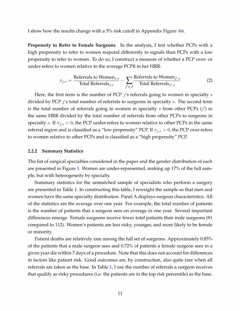
Propensity to Refer to Female Surgeons In the analysis, I test whether PCPs with ahigh propensity to refer to women respond differently to signals than PCPs with a lowpropensity to refer to women. To do so, I construct a measure of whether a PCP over- orunder-refers to women relative to the average PCPß in her HRR:

πj,s =Referrals to Womenj,s

Total Referralsj,s− ∑j′∈J

Referrals to Womenj′,sTotal Referralsj′,s

(2)

Here, the first term is the number of PCP j’s referrals going to women in specialty s

divided by PCP j’s total number of referrals to surgeons in specialty s. The second termis the total number of referrals going to women in specialty s from other PCPs (j′) inthe same HRR divided by the total number of referrals from other PCPs to surgeons inspecialty s. If πj,s < 0, the PCP under-refers to women relative to other PCPs in the samereferral region and is classified as a “low propensity” PCP. If πj,s > 0, the PCP over-refersto women relative to other PCPs and is classified as a “high propensity” PCP.

2.2.2 Summary Statistics

The list of surgical specialties considered in the paper and the gender distribution of eachare presented in Figure 1. Women are under-represented, making up 17% of the full sam-ple, but with heterogeneity by specialty.

Summary statistics for the unmatched sample of specialists who perform a surgeryare presented in Table 1. In constructing this table, I reweight the sample so that men andwomen have the same specialty distribution. Panel A displays surgeon characteristics. Allof the statistics are the average over one year. For example, the total number of patientsis the number of patients that a surgeon sees on average in one year. Several importantdifferences emerge. Female surgeons receive fewer total patients than male surgeons (81compared to 112). Women’s patients are less risky, younger, and more likely to be femaleor minority.

Patient deaths are relatively rare among the full set of surgeons. Approximately 0.85%of the patients that a male surgeon sees and 0.72% of patients a female surgeon sees in agiven year die within 7 days of a procedure. Note that this does not account for differencesin factors like patient risk. Good outcomes are, by construction, also quite rare when allreferrals are taken as the base. In Table 1, I use the number of referrals a surgeon receivesthat qualify as risky procedures (i.e. the patients are in the top risk percentile) as the base.

11

For both men and women, 26% of referrals they receive that qualify as risky will not resultin a death or rehospitalization.

Mean surgeon ability is also reported. Women have a slightly higher mean ability andslightly lower variance of ability, but the differences are small. Figure 2 plots the probabil-ity distribution function and the cumulative distribution function of surgeon ability. Thedistributions for men and women largely line up with one another.

Panel B presents summary statistics for PCPs, again measuring variables over thecourse of a year. PCPs refer to 15.5 different male surgeons and 2.5 different female sur-geons per year. For any given procedure, PCPs have relatively few surgeons whom theyrefer to, referring to 1.4 male surgeons per procedure and 0.2 female surgeons. Note thatthis is not the number of surgeons that are available to be referred to. Within the set ofspecialties that are included in the matched sample, PCPs have an average of 7 availablesurgeons to refer to in a given specialty.

3 Empirical Strategy

To understand how PCPs update their beliefs, I use an event study design to comparehow referrals to male and female surgeons change after good and bad patient outcomes.The previous section showed that male and female surgeons receive different types ofpatients. I therefore use a matching procedure to match men and women who have sim-ilar characteristics and are performing the same surgery on similar patients. This sectionfirst describes the matching procedure and shows that the resulting sample is balanced interms of both surgeon and patient characteristics. It then describes the event study design,estimating equations, and identification assumptions.

3.1 Matching Procedure

I carry out a coarsened-exact match for male and female surgeons on a set of patient andsurgeon characteristics.10 For this procedure, I start with the sample of all events, meaningthat surgeons can be included in the sample multiple times if they experience multipleevents. If a surgeon experiences multiple events with the same PCP, I only keep the firstinstance of an event. Before matching, I have a sample of 265,734 distinct surgeon-PCPpairs with bad events and 302,294 distinct pairs with good events. I then match male andfemale surgeons on variables measured over the four quarters before an event. I match

10This procedure involves matching surgeons exactly on the surgeon’s specialty, the procedure beingperformed, and the patient’s gender and race. The other variables are then divided into bins and surgeonsare matched across bins.

12

with replacement of individual surgeons and PCPs but allow each surgeon-PCP pair to bematched only once.

I match exactly on the surgeon’s specialty, the procedure being performed, and thepatient’s gender and minority status (white vs. non-white). Individuals for whom thereis no exact match for each of these categories are dropped. Procedures are identified viathe Current Procedural Terminology (CPT) code that the American Medical Associationmaintains to standardize medical service reporting. There are multiple “layers” of codingwith 19 broad parent groups of surgical procedures. Within a parent group, there are threeadditional layers, each identifying a procedure more uniquely. In Appendix A.1, I give anexample of what the layers look like for a sample parent group. I match on the second-finest layer, denoted by an asterisk in the appendix. Because there are slightly differentprocedures within each of these groups, I also match on the average risk of death foreach procedure. I am therefore either matching on the exact procedure or on very similarprocedures that differ slightly in treatment (for example, treating a humeral shaft fracturewith plates/screws versus treating a humeral shaft fracture with rods).

I match coarsely on the patient’s age and risk; the number and fraction of PCP j’sreferrals going to surgeon i prior to the event; the total number of referrals surgeon i

received from any PCP prior to the event; and surgeon experience, measured in terms ofthe number of years since the surgeon finished medical school and the number of specificprocedures the surgeon had completed prior to the event. Finally, I match on a PCP’soutside option, using the number of other surgeons available in surgeon i’s speciality inthe same HRR. I use an average of 9 bins for each variable.

Matching on patient age, gender, race, and risk attempts to minimize the differencesbetween patients that the surgeons see. Matching on past surgeries, referrals, and yearsof experience allows me to compare two surgeons with similar experience levels, bothin performing the procedure at hand and in their overall experience. Matching on thenumber of surgeons in the same specialty as surgeon i in PCP j’s referral region ensuresthat I am comparing PCPs who have similar outside options. Note that I do not requirethe matched surgeons to have the same referring PCP.

Tables 2 and 3 show that the final samples of matched male and female surgeons whoexperience bad and good events respectively are balanced. I end up with 7,757 surgeonmatches for bad events and 6,979 matches for good events.

13

3.2 Estimating Equations and Identification Assumptions

I briefly overview the main estimating equations and identification assumptions that Iuse in the analysis. The remaining estimating equations are presented with the results inSection 4.

Estimating Equations and Identification for Matched Male/Female Surgeon Pairs

To identify the impact of a good or bad event on referrals, I designate the quarter in whichan event occurs as quarter 0. I then sum the number of referrals a surgeon received fromthe referring PCP in each quarter, starting four quarters before the event and ending sixquarters after the event, and leaving out the patient referred for surgery. I stack the eventsof all PCP-surgeon pairs and estimate equation 3 below, where eventij,t−k is a dummyvariable indicating that an event occurred in quarter t and femi is a dummy variableindicating the surgeon is female:

Rijk =6∑k=−4

βkeventij,t−k +6∑k=−4

γk (eventij,t−k × femi) + θij + εijk (3)

The outcome variable, Rijk, is the number of referrals PCP j sends to surgeon i in quarterk. The coefficient γk tells us how a PCP’s reaction to an event changes when the surgeonis a woman.

I include PCP-surgeon match fixed effects, θij , to absorb any initial differences betweenmatches and cluster standard errors at the PCP-surgeon match level in case there are id-iosyncratic factors that are specific to a particular PCP-surgeon pair. This assumes thateach pair’s errors are uncorrelated with the errors of other pairs.

The main identification assumption is that women do not systematically receive dif-ferent types of patients or perform different procedures than men. For example, if womenreceive less risky patients, it would make sense that a PCP would update more about themthan about men after a bad event. Matching on patient characteristics, including patientrisk, as well as on the procedure code should alleviate this concern. However, furtherrobustness checks are presented in Section 5.

Estimating Equations and Identification for “Placebo” Surgeons

To understand what referral patterns between the PCP and the surgeon would have lookedlike in the absence of an event, I create a set of placebo surgeons who perform a surgerybut do not experience a good or bad event (e.g. they experience the expected outcome).

14

To do so, I use the matching procedure described in Section 3.1 to match female surgeonswho are identical on all observables and who receive observably similar patients, but oneof whom has a patient die while the other does not. I do the same for male surgeons. Forbad events, I am thus comparing surgeons who had a patient die (the treated surgeons) tothose who did not (the placebo surgeons) and for good events I am comparing surgeonswhose patient lived (treated) to those whose patient dies or is re-hospitalized (placebo).Balance tables are presented in Appendix Table C.

To quantify the impact an event has on referrals to a surgeon, I estimate

Rijk =6∑k=−4

βksurgeryij,t−k +6∑k=−4

γk (surgeryij,t−k × eventk) + θij + εijk (4)

on the matched female and matched male samples separately. The variable surgeryij,t−kis a dummy variable that equals one during the quarter of the surgery and eventk is adummy variable indicating that a good or bad event occurred. All other variables aredefined as before.

Estimating Equations for Spillovers

In the analysis I test whether one surgeon’s performance affects how the PCP updatesabout other surgeons. To do so, I estimate

fijgsk =6∑k=−4

βkeventij,t−k +6∑k=−4

γk (eventij,t−k × femi) + δavailablejs + θij + εijgsk (5)

separately on the samples of male and female surgeons. The outcome variable, fijgsk, isthe fraction of PCP j’s new referrals going to surgeons in group g (men or women) inspecialty s in quarter k, when surgeon i performs a surgery in quarter t. The measureleaves out referrals going to the performing surgeon i. Other variables driving the PCPto refer less to women therefore have to change at the time of the event to explain thechanges in the PCP’s behavior. For example, if other women in the PCP’s HRR are lessskilled or have full schedules, it is unlikely that the PCP referred to them before the eventoccured so the change in the fraction of referrals going to other women should not change.

I control for the fraction of available surgeons (availablejs) who are of the same gen-der and in the same specialty as the performing surgeon to ensure that the results arenot driven by constraints in PCPs’ surgeon options. The result of this estimation tell uswhether PCPs change their beliefs about other female (male) surgeons after one of theirpatient lives or dies under the care of a female (male) surgeon.

15

Variables Correlated with PCP’s Reaction

To understand what drives a PCP’s reaction, I correlate several variables with the changein referrals from a PCP to a surgeon. Specifically, I estimate

Rijt = β1Femi + β2Postt + β3V ar+ β4(Femi × Postt) + β5(Femi × V ar)

β6(Postt × V ar) + β7(Femi × Postt × V ar) + ∑Xk∈X

Xijtt+ θij + εijt (6)

where Postt is a dummy equalling one for quarters after the event occurs and V ar is thevariable being tested for correlation with the PCP’s response. A time trend and time trendinteractions (∑Xk∈X Xijtt) with the variables X = {Postt, Femi, V ar} are also included.

4 Results

The empirical analysis uncovers two asymmetries in how PCPs react to signals. First,there is an individual-level asymmetry. PCPs respond more to good signals if the surgeonis male and more to bad signals if the surgeon is female. Comparing surgeons who experi-enced a good or bad outcome with the placebo surgeons who did not, I find that while thereferral path for men and women would have been similar had the event not occurred,women receive far fewer referrals following a bad outcome than they otherwise wouldhave. Conversely, men receive more referrals after a good outcome than they otherwisewould have. Second, there is an asymmetry at the group level. PCPs update their beliefsabout other women after receiving a signal from an individual woman but do not updateabout other men after receiving a signal from one man.

PCPs who just began a referral relationship with a particular surgeon react the strongest.The longer is a PCP’s referral relationship with a surgeon, the less that PCP reacts to pa-tient outcomes. Further, the gender gap in PCPs’ responses is decreasing in the length ofthe referral relationship. In what follows, I therefore focus primarily on PCPs and sur-geons who just began a referral relationship (i.e. where the PCP had sent fewer than10 referrals prior to the event), as the asymmetric response is concentrated among thesePCPs and surgeons. However, I show how the results depend on the length of the referralrelationship in Section 4.2.1.

16

4.1 Responses to Signals

4.1.1 Updating after a Bad Event

This section documents the referring PCP’s reaction to a patient death. Because I matchmale and female surgeons on both the number and fraction of referrals they received froma PCP before an event occurs, I am comparing two surgeons for whom PCPs have roughlythe same beliefs.11

Figure 3 documents how PCPs respond to a patient death, plotting the quarterly coef-ficients βk and βk + γk for k ∈ {−4, 6} from estimating equation 3. In this figure, PCP j

refers patient p to surgeon i. Surgeon i performs the surgery in quarter 0 and the patientdies within 7 days of the surgery. Coefficients are plotted relative to the number of refer-rals the surgeon received from PCP j in the quarter before the event (k = −1). Both maleand female surgeons were receiving 0.65 referrals in k = −1 from their referring PCP.

The figure shows that before the patient death, the surgeon receives an increasing num-ber of referrals from the PCP as they have just started their referrals relationship. Whenthe death occurs in quarter 0, the PCP refers less to the surgeon, with a marked dropin referrals occurring if the surgeon is female. Controlling for time trends, men receive0.101 more referrals in the quarters after the death relative to the quarter before the death,whereas women receive 0.222 fewer referrals after the death relative to the quarter before.12

The gap in referrals that emerges between male and female surgeons is significant at the1% level and persists up to a year and a half following the death. To put these numbersinto perspective, a male surgeon would have to have three patient deaths to be treated thesame as a female surgeon. Given the rarity of patient deaths, this difference is substantial.The results are summarized in column 1 of Table 4.

I also find a change in the types of patients and procedures that the PCP refers in thefuture. In Figure 5, I re-estimate equation 3 but use the average risk of patients that PCP jrefers to surgeon i in quarter k as the dependent variable. There is no significant change inthe riskiness of patients that PCPs send to men. However, women start to receive patientsthat are 0.28 standard deviations less risky after a death. Similarly, women are referredprocedures that are 0.041 standard deviations less risky than what they received before thedeath. The impact that this has on surgeon pay and skill accumulation is further discussedin Section 6

To further quantify the impact that a death has on male and female surgeons, I showwhat the referral path would have looked like in the absence of a death using the matched

11This is assuming that referrals are a function of a PCP’s belief about a surgeon’s average ability, a claimthat I further explore in Section 7

12See Table 4, column 1.

17

sample of treated/placebo surgeons described in Section 3. The matched surgeons areidentical on observables and receive patients with similar risk levels and demographics,but one surgeon experiences a patient death while the other does not. It is worth notingthat the absence of a death is not equivalent to the PCP receiving no signal from a surgeon.The fact that the patient lives is in itself a good signal. I am therefore not comparing asurgeon who sends a bad signal to one who does not send a signal.

Figure 4 plots the results from estimating equation 4 separately for male and femalesurgeons. In both figures, the estimates for the placebo surgeons indicate that the numberof referrals to male and female surgeons would have continued to grow at a similar ratehad the patient not died. However, the gap between the actual and “projected” numberof referrals is smaller for men (top panel). Men who experience a patient death receive0.22 fewer referrals each quarter than they would have if the patient lived. The F-statisticfor the joint significance of δ1-δ6 is 2.48. Women who experience a patient death, shownin the bottom panel, receive 0.6 fewer referrals each quarter (with an F-statistic of 15.88).PCPs thus seem to update their beliefs downward about both male and female surgeons,but by a larger amount when the surgeon is female.

The difference in outcomes between women and men who do and do not experiencea patient death is summarized in a difference-in-differences plot shown in panel (c) ofFigure 4. There is no difference in the referral path between male and female surgeonswho do not experience a patient death (grey circles) but women who experience a patientdeath receive approximately 0.3 fewer referrals per quarter than men who experience adeath (green triangles).

4.1.2 Updating after a Good Event

It is possible that PCPs react more to bad signals from women because the variance ofwomen’s ability is larger. If this is true, PCPs should react strongly to good signals fromwomen as well.13 I now test how PCPs react to “unexpectedly good” outcomes, defined asthe top 1% of the riskiest patient-procedures pairs for which no death or re-hospitalizationoccurred. The quarterly coefficients from estimating equation 3 as well as the placebooutcomes are presented in Figure 6.

Opposite to their reaction to a death, PCPs respond more strongly when the surgeon ismale than when the surgeon is female. While referrals to both male and female surgeonsincrease, they increase by a significantly larger amount for male surgeons. Controlling fortime trends, men receive roughly 0.6 more referrals than they did in the period before the

13This is assuming that ability is distributed according to a symmetric distribution. Such assumptions areformally analyzed in Section 7

18

good event whereas women receive 0.35 more referrals, a difference that is significant atthe 5% level (see Table 4, column 2 for a summary of effects). A PCP’s response to goodsignals stands in stark contrast to how PCPs react to bad signals, where their response tomale surgeons is muted.

Relative to the sample of surgeons who did not experience a good outcome, men re-ceive 0.25 more referrals per quarter than they otherwise would have while women re-ceive 0.15 more. Note that a difference in the number of referrals to men and women whodo not experience a good outcome also emerges as the expected outcome in this case is ahospital readmission or death. Although a re-hospitalization is expected, women still re-ceive slightly fewer referrals than men do after the surgery.14 The difference-in-differencescoefficients are plotted in the bottom panel of Figure 6.

4.1.3 Spillovers: Updating about Other Surgeons

I now turn to the question of whether a PCP’s experience with one surgeon influencesthat PCP’s beliefs about other surgeons of the same gender. Figure 7 plots the quarterlycoefficients from estimating equation 5 where the event is a patient death.

The outcome in the top figure is the fraction of a PCP’s referrals going to surgeonsthe PCP hasn’t referred to before who are the same gender and in the same specialty asthe performing surgeon. I focus on new referral relationships as a PCP’s experience withone surgeon does not significantly impact her beliefs about another surgeon she has beenreferring to for some time. This is shown in Appendix Figure A1 where PCPs who have along referral history with a particular surgeon do not change their referrals to that surgeonafter having a bad experience with surgeon i.

In cases where a female surgeon has a patient die (the red triangles), the PCP becomesless likely to form referral relationships with female surgeons in the future. However,PCPs do not change their propensity to form new referral relationships with male sur-geons after a patient dies under a man (the blue circles). Men appear to be treated asindividuals while information about one woman in specialty s affects the PCP’s beliefsabout other women in specialty s.

The bottom figure shows the change in a PCP’s referrals to new surgeons of the samegender but in different specialties than the performing surgeon. PCPs slightly reduce thefraction of their referrals going to female surgeons in other specialties but the post-deathcoefficients are jointly insignificant.

The spillover results are summarized in columns 3 and 4 of Table 5. Relative to the

14In Section 4.2.3, I show how PCPs’ responses to deaths depend on patient risk as well as several otherfactors.

19

mean fraction of referrals going to new female surgeons in the same specialty, the declinein referrals is substantial. The fraction of a PCP’s referrals going to new women in thesame specialty as the performing surgeon declines by 53% (column 1). The fraction goingto new women in other specialties (column 3) declines by 20% (but again, this result isinsignificant).

Interestingly, PCPs do not appear to treat women as a group when a woman performswell. Column 2 of Table 5 shows the spillovers to other women after a female surgeonhas a good patient outcome. The coefficient on the female×post interaction variable ispositive but insignificant.15 It is possible, though, that a PCP updates her beliefs aboutother female surgeons upward but continues to only refer to the performing surgeon.

These results also provide evidence that the drop in referrals is not simply due to fe-male surgeons changing their behavior. A large literature shows that women are less likelyto be overconfident than men (Lichtenstein, Fischhoff, and Phillips, 1982; Beyer, 1990; Bar-ber and Odean, 2001). It is possible that female surgeons turn away more referrals aftera patient death if the event hurts their confidence. The fact that PCPs are changing theirbehavior toward other female surgeons, though, suggests that at least part of the changeis due to PCPs.

4.1.4 Information Spillovers to Other PCPs

The implications that asymmetric updating has on a surgeon’s career depends in part onwhether information about an event spreads to other PCPs. I test whether other PCPsreact to a bad event in Figure 8. I plot the coefficients from estimating

Ri,−j,k =6∑k=−4

βkeventij,t−k +6∑k=−4

γk(eventij′,t−k × femi) + θij + εijk (7)

where eventij,t−k is still a dummy variable indicating that a bad event occurred betweenPCP j and surgeon i, but the outcome variable is the number of referrals that surgeon i

receives from other PCPs (excluding j). I consider two outcome variables: the number ofreferrals going from other members of PCP j’s group practice and the number of referralsfrom PCPs outside of PCP j’s practice.

Panel (a) plots the coefficients when the outcome variable is the number of referrals tothe performing surgeon from other members of PCP j’s group. I restrict the group prac-tices to be those containing at most 20 members. This is done to account for the fact that

15Appendix Figure A2 plots the coefficients from estimating equation 5 using good events. There are nosignificant positive spillovers to other women or men in the same specialty as the performing surgeon.

20

many group practices defined in the Medicare data cover groups with branches in multi-ple regions. It is therefore unclear whether group practices with many members are largepractices in one geographic location or normal-sized practices with multiple branches.There is a small decline in the number of referrals from other members of small grouppractices. Female PCPs receive on average 0.5 fewer referrals per quarter after a badevent than before, but the coefficients in quarters 1 through 6 are jointly insignificantlydifferent from zero. Male surgeons, on the other hand, continue to receive referrals fromthe referring PCP’s practice.

Panel (b) shows the change in referrals from PCPs outside of PCP j’s practice but inthe same HRR. Here we see no impact on the number of referrals the surgeon receives.Both women and men continue to receive referrals from PCPs outside of the referringPCP’s practice, suggesting that information does not spread or that PCPs do not act onthis information.

4.2 What Influences a PCP’s Reaction to a Signal?

I have shown that PCPs respond differently to a given patient outcome depending onthe surgeon’s gender. PCPs lower referrals to female surgeons more than male surgeonsafter a bad outcome and increase referrals more to male surgeons than to female surgeonsafter a good outcome. I now explore other factors that influence a PCP’s reaction, findingtwo main drivers. First, PCPs’ reactions to signals are weaker the more signals they havereceived from a surgeon in the past. PCPs who have received many signals from a womanprior to the event are also more likely to treat her the same as a man. Second, PCPs witha high propensity to refer to women before the event treat men and women more equally- e.g. exhibit less asymmetric updating - than PCPs with a low propensity to refer towomen.

4.2.1 Referral History with Surgeon

So far I have restricted the analysis to PCP-surgeon pairs in which the PCP has referred atmost 10 patients to the surgeon before the event. This concentrates the analysis on PCPswho are presumably learning about a particular surgeon. If PCPs learn about surgeonsover time, they will become more certain in their beliefs about a surgeon’s ability thelonger they have been referring to one. To test how a PCP’s reaction changes with thelength of her relationship with a surgeon, I estimate equation 6 where the independentvariable of interest is the number of referrals that PCP j sent to surgeon i in the year

21

before the event.16 I estimate equation 6 on the set of matched surgeons who have had upto 50 prior referrals from a given PCP. I am still comparing male and female surgeons whoreceive the same number and fraction of referrals before an event occurs, but am lookingat how a PCP’s reaction changes the more a PCP has worked with a surgeon.

The results are presented in columns 1 and 3 of Table 6. Pre-Referrals is the number ofpatient referrals that PCP j sent to surgeon i before the bad (column 1) or good (column3) event. These “pre-referrals” are referrals that ended well: the patient did not die andwas not readmitted to the hospital. I am therefore measuring how an additional referralthat ended in a good patient outcome affects the PCP’s response. An additional referralfrom a PCP to a surgeon reduces the PCP’s negative response to a death by 0.014 referralsper quarter for male surgeons and 0.022 referrals per quarter for female surgeons, therebydiminishing the gender gap in PCP response. Female surgeons need to have sent 22 goodsignals (performed 22 procedures that went well) to a PCP in the year before the event forthere to be no gender gap in the PCP’s response.

An additional referral mitigates a PCP’s positive reaction to a good outcome when thesurgeon is male but does not change the positive response when the surgeon is female,again leading to more equal responses. These results suggest that PCPs learn about sur-geons, becoming more certain in their beliefs about a surgeon’s ability over time. Any biasthat they exhibit comes out only when working with new surgeons.

4.2.2 PCP Response and Referral History with Other Surgeons

The previous section showed that the longer the referral relationship between a PCP anda surgeon, the more muted the PCP’s response to an event is. It is unclear, though, howa PCP’s response is influenced by her referral history with other surgeons of the samegender as the performing surgeon. For example, a PCP who has favorable beliefs aboutwomen and who sends a large volume of referrals to them presumably has more informa-tion about women. That PCP may not react as much to new signals. Depending on theshape of the PCP’s priors, though, a surgeon who thought women were very good andwas consequently surprised to see a patient die under a woman might drastically reviseher beliefs.

To understand how a PCP’s response varies with her referral history with other sur-geons, I again estimate equation 6 and use the “propensity to refer to women” variabledescribed in Section 2 as the main explanatory variable. A PCP’s propensity to refer towomen is measured as the difference between the fraction of her referrals going to women

16I do not look at the full referral history as the data is cut off in 2008. However, these two measuresshould be correlated.

22

in a particular specialty and the average fraction going to women of other PCPs in thesame referral area. I then define a variable, High Propensity, that equals one if a PCP sendsa greater fraction of her referrals to women within a given specialty than the average PCPin her referral region.

The results are presented in columns 2 and 4 of Table 6. PCPs with a high propensityto refer to women react less negatively after bad outcomes and more positively after goodoutcomes. The gender gap in the PCP’s reaction shrinks by 22% if a PCP has a highpropensity to refer to women.

4.2.3 Other Variables Influencing PCP’s Reaction

I also test whether a PCP’s outside option, surgeon and PCP experience, and PCP genderinfluence the PCP’s reaction to a signal.

Outside Options It is plausible that a PCP who has many possible surgeons she canrefer to would have a stronger response to a patient death as it is easier for her to shiftto a new surgeon. To test whether a PCP’s outside option matters, I use the number ofsurgeons in the same specialty as the performing surgeon in the referring PCP’s HRR. Theresults from estimating equation 6 are presented in Column 1 of Table 7, the x-variable ofinterest is PCP j’s outside option. There is a small impact of having more outside optionsbut the result is statistically insignificant.

Experience I look at both the PCP’s and the surgeon’s experience, measured as the num-ber of years since they graduated from medical school, to understand whether experienceinfluences a PCP’s reaction to signal. I again estimate equation 6 but include Experi,t (thesurgeon’s experience at the time of the event) or Experj,t (the PCP’s experience) as themain independent variable. I also include squared experience terms to allow for non-linearities in the doctor’s response. The results are presented in columns 2 and 3 of Table7. There is no significant relationship between either doctor’s experience and the PCP’sreaction. A PCP’s experience working with a particular surgeon seems to matter morethan absolute years of experience.

PCP Gender The evidence on how women evaluate other women is mixed. For exam-ple, Casadevall and Handelsman (2014) find that having a woman on a convening teamfor scientific conferences increases the proportion of invited women. Bagues et al. (2017),however, find that women evaluating tenure cases do not favor female candidate and thatmen in fact become harsher in their evaluations in the presence of a female evaluator.

23

I find no significant evidence that male and female PCPs treat female surgeons dif-ferently. In column 4 of Table 6, a female dummy indicating that the PCP is female isincluded as the independent variable of interest. The point estimate on the triple interac-tion between Female, Post, and Female PCP is positive, suggesting that female PCPs mightbe easier on female surgeons than male PCPs, but the result is noisy and I cannot rule outno or negative effects.

Summary of Results

In sum, I look at the impact of two signals, good and bad, on two sets of outcomes for maleand female surgeons: referrals to the performing surgeon and referrals to other surgeonsof the same gender. The following table, which draws from Tables 4 and 5, shows theaverage post effect of an event on referrals to individual surgeons and to other surgeons.

Performing Surgeon Other SurgeonsMale Female Male Female

Bad Outcome 0.101 -0.222 ∅ -0.079

Good Outcome 0.604 0.346 ∅ ∅

5 Alternative Interpretations

Before discussing what the empirical findings tell us about how PCPs update their beliefs,I explore three alternative interpretations of the results. I show that differences in unob-servable risk, differences in the predictiveness of events for future events, and changes inthe PCP’s behavior cannot account for the findings.

5.1 Differences in Patient Risk

Although I match on observable patient risk, there could be unobservable factors influenc-ing risk. If female surgeons receive less risky patients, deaths are surprising and survivalsare unsurprising, meaning that PCPs respond strongly to deaths and weakly to survivals.Here, I put bounds on what the unobservable risk difference between male and femalesurgeons’ patients would have to be to justify the degree of differential updating.

In Figure 9, I plot the regression coefficients β1 and β1 + β2 + β3 from estimating

∆Rijp = β1Riskp + β2(Riskp × Femi) + β3Femi + θi + εijp (8)

24

where ∆Rijp is the change in referrals from PCP j to surgeon i before and after patient p’sdeath, and Riskp is the patient p’s observed risk level. The coefficient β2 tells us what thedifference in unobserved risk between a female surgeon’s and a male surgeon’s patientwould have to be to account for the gender difference in the PCP’s reaction.

While PCPs respond to patient risk regardless of surgeon gender, they respond muchmore when the surgeon is female. Figure 9 shows that a male surgeon with a patient inthe bottom risk decile experiences a drop in referrals equivalent to what a female surgeonwith a patient in the 7th decile receives. Thus, any differences in unobserved risk wouldhave to be large enough to move a patient that a male surgeon sees from being in thebottom 10th percentile of patient risk to the top 70th percentile of observed risk, a largedifference.

5.2 Are Outcomes Differentially Predictive of Future Outcomes?

A PCP’s behavior is also be justified if bad events are predictive of future bad events forfemale surgeons and good events are predictive of future good events for male surgeons.To test this hypothesis, I estimate

P(Eventi = 1|Xi,Xpt,Xi,p′) = β1Femi + β2FutRefsi+X′iγ + αlog(PastRiskp)+

δlog(FutRiskp′) + εip

on the matched samples of surgeons who experienced a bad or good event. The outcomevariable is the probability that surgeon i has another event in the future under any PCP(not just PCP j). I condition on the number of referrals the surgeon receives in the fu-ture from all PCPs (FutRefsi) as well as the log of future patient risk (log(FutRiskp′)). Ialso control for the performing surgeon’s characteristics (X ′i), including experience, spe-cialty, and work history17, as well as the log of the surgeon’s past patients’ risk levels(log(PastRiskp)).

The results are presented in Table 8. I find no evidence that patient deaths are morepredictive of future deaths for female surgeons than for male surgeons. In fact, womenare less likely to have future patients die even conditional on the risk of future patients.If PCPs are responding to an unobservable factor, it is not something that influences thefuture performance of surgeons.

17This includes the number of patients seen before the death.

25

5.3 Do PCPs Stop Referring for Certain Procedures?

An additional concern is that PCPs stop referring patients for a particular surgery aftera patient dies. For example, Keating et al. (2017) find that doctors who refer a patientfor a colonoscopy are less likely to refer patients for that procedure if the patient has anextreme adverse outcome. However, the effect is short-lived as PCPs begin referring forthe procedure again, and at the same rate as before, one quarter after the adverse outcome.Nevertheless, if women tend to specialize in one type of surgery while men perform manydifferent surgeries, the drop in referrals to women could be due to the PCP changing thetypes of procedures she refers.

I test this by looking at how referrals for the surgery that was performed change aftera patient death. Specifically, I estimate

Sjk =6∑k=−4

βkeventij,t−k +6∑k=−4

γk (eventij,t−k × Femi) + θij + εij (9)

where S is the surgery that was being performed on the patient who died and Sjk is thenumber of those surgeries that PCP j refers to any surgeon in quarter k.

The results are shown in Appendix Figure A3. For female surgeons, the coefficientson all quarters before and after the event are precise zeros, indicating that the PCP doesnot change her referral patterns for the surgery in question. For male surgeons, there is asmall drop in the number of referrals the PCP gives for the procedure in question in k = 1but the PCP’s referrals revert back to the mean shortly thereafter.

I also show that the PCP decreases referrals to surgeon i for all procedures, not just theone that was being performed on the patient who died. In Appendix Figure A4, I plot thecoefficients from estimating

OtherRefijk =6∑k=−4

βkeventij,t−k +6∑k=−4

γk (eventij,t−k × Femi) + θij + εij (10)

where the outcome variable, OtherRefijk, is the number of referrals that the PCP sendsto the surgeon aside from the procedure that was being performed on the patient whodied. The results are noisy as PCPs typically only refer to a surgeon for a particular pro-cedure, but the patterns are the same. Referrals for other procedures drop for both menand women but by a greater amount for women. The coefficients for female surgeons aresignificantly different from those for male surgeons at the 10% level.

26

6 Welfare Analysis and Career Effects

6.1 Physician Quality

If asymmetric updating distorts a PCP’s belief about a surgeon’s ability, PCPs may switchaway from high ability female surgeons after receiving negative signals. For example,if PCPs have some cutoff ability, below which they do not refer to a surgeon, PCPs willstop referring to female surgeons earlier than similar men. The average ability of malesurgeons they refer to will eventually be lower than that of the female surgeons they referto.

To test whether asymmetric updating affects the average quality of surgeons a PCPrefers to, I use the definition of surgeon ability described in Section 2. I then calculate theaverage ability of all surgeons a PCP refers to in each quarter and plot how it changesafter a bad event under one surgeon. If PCPs give male surgeons too many chances tomake mistakes and female surgeons too few chances, average surgeon ability will declineafter a patient death as PCPs move away from potentially qualified female surgeons topotentially less qualified male surgeons.

Figure 10 plots the quarterly coefficients from estimating

ajk =6∑k=−4

βkeventij,t−k +6∑k=−4

βk(eventij,t−k × femi) + θij + εijk

where ajk is the average ability of the surgeons that PCP j refers to in quarter k. There isno significant change in the quality of surgeons that PCPs refer to when the performingsurgeon is a man. However, when the performing surgeon is a woman, the average sur-geon quality falls by approximately 0.1 standard deviations in the year following a death,although these results are only marginally significant at the 10% level. However, they pro-vide suggestive evidence that PCPs may be misestimating female surgeons’ abilities afterdeaths and switch from some high ability female surgeons to other lower ability surgeons.

6.2 Surgeon Pay and Skill Accumulation

I now turn to the impact that asymmetric updating has on surgeons’ career trajectories. InSection 4, I find limited evidence that information about a patient death spreads to otherPCPs. There is a small decline in the number of referrals that women receive from othermembers of the referring PCP’s group practice, provided the practice is small. However,this decline is statistically indistinguishable from zero. As such, I abstract from changes inother PCPs’ behavior and focus on the impact that asymmetric updating by the referring

27

PCP has on pay and skill accumulation.Numerous papers have documented a pay gap between male and female physicians.18.

Closely related to this paper, Zeltzer (2016) decomposes the Medicare earnings gap, show-ing that in the raw data, women earn 48% less than men. About a third of the gap can thenbe explained by difference in the specialties men and women select into. Controlling forcareer interruptions and differences in experience and education, Zeltzer shows that gen-der homophily in referrals explains an additional 15% of the gap. However, the remainderof the gap remains unaccounted for.

Here, I provide an additional mechanism that contributes to the gap, but do not quan-tify the contribution. It is difficult to estimate the full impact that asymmetric updatinghas on the surgeon pay gap as I look at two specific and relatively infrequent events. Sur-geons experience less than one bad outcome per year, for example. Furthermore, PCPsexhibit asymmetric updating when they are starting new referral relationships, so the rel-evant baseline pay gap for comparison is the gap that exists between men and women atthe beginning of their careers or who have moved. I therefore show that asymmetric up-dating creates a wedge between male and female pay but do not speculate on its relativeimportance in explaining the overall surgeon pay gap.

Figure 11 shows the change in Medicare payments following a patient death, plottingthe quarterly coefficients from estimating

Payijk =6∑k=−4

βkDeathij,t−k +6∑k=−4

γk (Deathij,t−k × femi) + θij + εijk (11)

on the sample of matched surgeons who experience a patient death. The outcome vari-able, Payijk, is the total quarterly Medicare pay that surgeon i receives from PCP j’s refer-rals in quarter k. A patient death occurs in k = 0.

Because I have matched on a number of variables that influence the gender pay gap(such as volume of referrals, experience, and specialty), there is a small but statisticallyinsignificant difference in male and female surgeon pay before the death. After the death,a gap of approximately $140 per quarter emerges. Column 3 of Table 4 summarizes theeffect, showing that women lose approximately 60% of their Medicare billings from thereferring PCP while men lose 30%. Women incur a substantial pay penalty from the re-ferring PCP but given that other PCPs do not change their behavior much, women do notexperience a substantial pay penalty overall.

Column 4 of Table 4 shows the impact of a good patient outcome on Medicare pay.Men receive a 36% increase in quarterly Medicare billings while women receive a 19%

18See, for example, Ly et al. (2016), Lo Sasso et al. (2011), and Sasser (2005)

28

increase, although the difference is statistically insignificant.A second channel through which asymmetric updating can influence women’s careers

is through skill acquisition. In Section 4, I showed that female surgeons who still receivereferrals after a patient death receive easier cases, either with less risky patients or lessrisky procedures. Since learning-by-doing is important for surgeon learning19, asymmet-ric updating might impact women’s skill accumulation which can also influence futurepay as well as their career trajectory.

7 Theoretical Framework

This section sets up a theoretical framework to link the empirical results to belief updat-ing, answering whether and under what conditions the observed behavior is in line withBayesian updating.

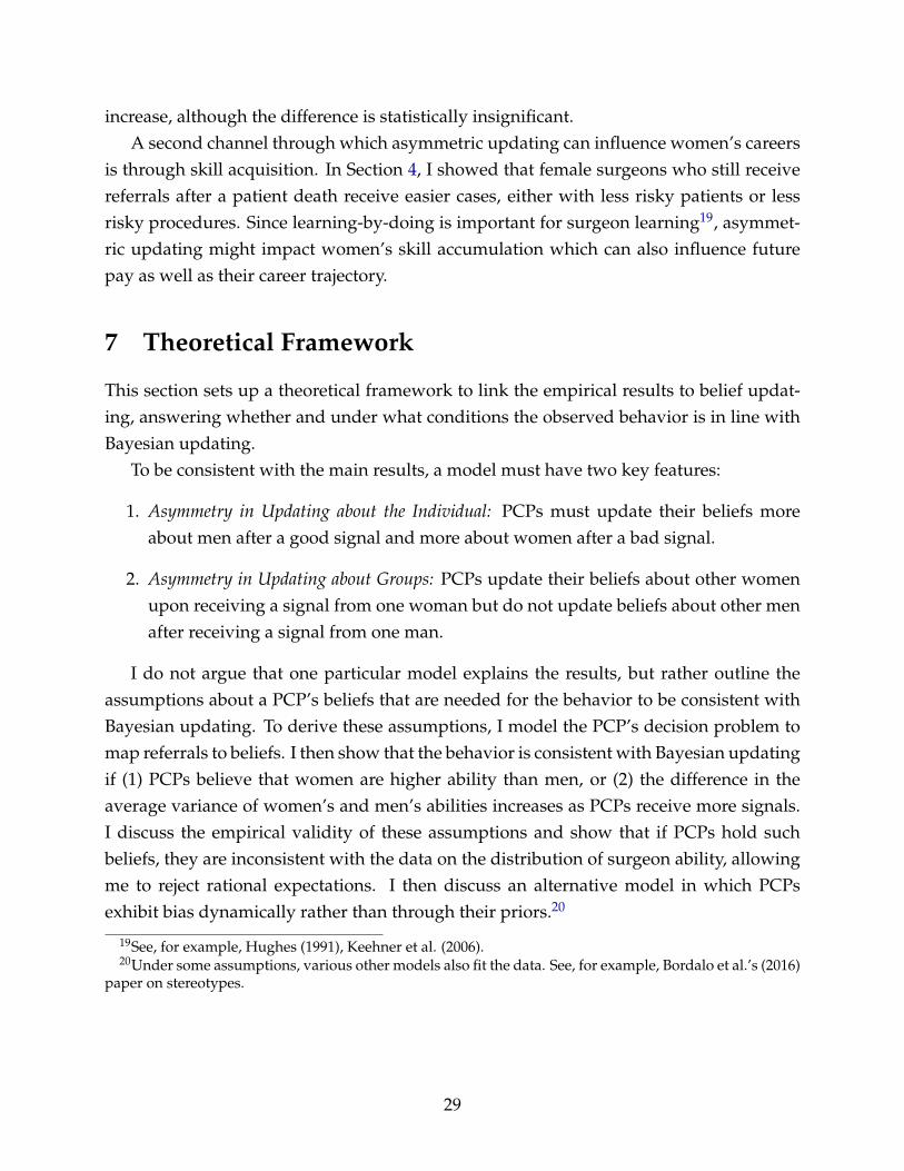
To be consistent with the main results, a model must have two key features:

1. Asymmetry in Updating about the Individual: PCPs must update their beliefs moreabout men after a good signal and more about women after a bad signal.

2. Asymmetry in Updating about Groups: PCPs update their beliefs about other womenupon receiving a signal from one woman but do not update beliefs about other menafter receiving a signal from one man.

I do not argue that one particular model explains the results, but rather outline theassumptions about a PCP’s beliefs that are needed for the behavior to be consistent withBayesian updating. To derive these assumptions, I model the PCP’s decision problem tomap referrals to beliefs. I then show that the behavior is consistent with Bayesian updatingif (1) PCPs believe that women are higher ability than men, or (2) the difference in theaverage variance of women’s and men’s abilities increases as PCPs receive more signals.I discuss the empirical validity of these assumptions and show that if PCPs hold suchbeliefs, they are inconsistent with the data on the distribution of surgeon ability, allowingme to reject rational expectations. I then discuss an alternative model in which PCPsexhibit bias dynamically rather than through their priors.20

19See, for example, Hughes (1991), Keehner et al. (2006).20Under some assumptions, various other models also fit the data. See, for example, Bordalo et al.’s (2016)

paper on stereotypes.

29

7.1 PCP’s Decision Problem

Setup

I follow the setup in Zeltzer (2016). There are two types of agents, PCPs and surgeons.PCPs, denoted j ∈ J , decide which surgeon, i ∈ Ij , to refer a patient to where Ij is thepool of surgeons available to j. Surgeons belong to an identifiable group g ∈ {m,w} (menor women) and their ability, ai, is unknown to the PCP. In period t = 0, PCPs have a priorprobability distribution over a surgeon’s ability ai,t ∼ f(ai,σ2

i ) where ai is the PCP’s priorabout surgeon i’s average ability. In time 0, the PCP’s prior is based on her beliefs aboutthe group: ai,0 = ag. Similarly, σ2

i is the variance and σ2i = σ2

g in t = 0. I assume that f hasa defined mean and variance but do not place restrictions on higher-level moments.

After receiving a patient, surgeons draw and send a signal (a patient outcome). Tomatch the data, I assume that signals can be either good or bad: s ∈ {sG, sB}.21 Theprobability of drawing each type of signal depends on a surgeon’s ability, with higherability surgeons being more likely to draw a good signal. Specifically, let the probabilitythat a member from group g draws a signal s be P(s|g) = ∑i∈g P(s|ai)f(ai)da.

PCPs want to maximize patient utility by referring to the best available surgeon subjectto factors like patient preferences and wait times. PCP j chooses a surgeon i to maximize

argmaxi∈IjUp(a) = βE[ai,t|ai, g, s]− λσ2i,t + εipt (12)

where ai,t−1 is the PCP’s prior about surgeon i’s mean ability, where i belongs to groupg ∈ {m,w}. The constant λ represents risk preferences and εipt represents the idiosyncraticfactors discussed above. The PCP is thus trying to choose the surgeon with the highestexpected ability, the first term; trading off the variance of ability, the second term; andsubject to idiosyncratic factors, the third term.

Assuming εipt is independently and identically distributed according to the extremevalue distribution, we can write equation 12 in terms of the logit probability,

P(Rji,p,t = 1|ai,g,t−1) =eνij

∑i′∈I eνi′j

(13)

where Rji,p,t = 1 if the PCP refers patient p to surgeon i in time t, and νij = βE[ai,t|ai, s]−

21The model can be extended to include a set of finitely many ordered signals and the results do notchange.

30

λσ2i,t. PCP j’s total number of referrals to surgeon i in period t can then be written as

Rtotalijt = nt ·eνij

∑i′∈I eνi′j

where nt is the number of patients that the PCP refers to surgeon i in time t the surgeon’scapacity constraint has not been reached.

Aside from idiosyncratic factors like patient preferences, two main variables influencethe PCP’s referral choice in this model: beliefs about ability (E[ai,t]) and the variance ofability (σ2

i,t). Referrals are increasing in the surgeon’s expected ability and decreasing inthe surgeon’s expected variance of ability.22

I consider each case in turn. I first look at how Bayesian PCPs react to signals if theyonly care about mean ability, placing no restrictions on higher-order moments of the abil-ity distribution. I then consider how PCPs react if they have risk preferences and careabout the variance of ability.

7.2 Bayesian Updating: PCP Cares about Mean Ability

Recall that PCPs have the prior probability distribution ai,t ∼ f(ai,σ2i ) over a surgeon’s

ability. If a PCP only cares about mean ability, she chooses i to maximizeUp(a) = βE[ai,t|ai, g, s]+εip, which is equation 12 setting λ = 0. Holding the PCP’s beliefs about other surgeonsconstant, the change in referrals after a signal is then

∆Rijt =(nt − nt−1) · eβ(E[ai,t|ai,t−1,g,s]−ai,t−1)

∑i′∈S eβai′,t−1

(14)

Empirically, the change in referrals to women is larger after a bad signal and smaller aftera good signal compared to the change in referrals to men. For this to be true, it must bethat E[ai,t|s,w]− ai,w ≤ E[ai,t|s,m]− ai,m in equation 14. This is possible under Bayesianupdating when PCPs believe that women have higher average ability than men.

Consider the following proposition:

Proposition 1. If PCPs are Bayesian and the following statements are true:

1. E[ai|sG, g] > E[ai|sB, g]

2. E[ai,t|s,w]− ai,w ≤ E[ai,t|s,m]− ai,m22This assumes risk aversion in which a PCP prefers to refer to a surgeon who produces average outcomes

for sure than one who produces either very good or very bad outcomes with some probability. There may becases in which a PCP would prefer to refer to a surgeon with a high expected σ2 instead of a “safe” option,but I abstract from this case here.

31

then it must be that P(sG|w)P(sG|m)

> 1.

Proof. See Appendix B.

Proposition 1 states that if expected ability is increasing in the signal and that thechange in beliefs about women’s ability are always more negative than the change in be-liefs about men’s ability, then women must have a higher average ability than men, whichis equivalent to women having to send more good signals. Intuitively, if a Bayesian PCPbelieves that women are more likely to send good signals, any good signal is going to beclose to the PCP’s prior and she will not update her beliefs much. In contrast, when a mansends a good signal, the signal is far from the PCP’s prior, leading her to update more.Similarly, if a woman sends a bad signal, the PCP will update much more than she doesabout a man, whom the PCP already believes to be low ability.

Discussion of Assumptions

If PCPs believe that women are higher ability than men and PCPs only care about meanability, equation 12 implies that women should receive at least as many referrals as mendo. Empirically, female surgeons receive 10% of referrals while they make up 17% of thesurgeon population. Adjusting for the fact that women work fewer hours than men, theyshould receive at least 14% of referrals if PCPs refer to men and woman at equal rates.23.While the difference is small, female surgeons are under-referred to even after adjustingfor work hours.

Theoretically, a cost of referring to women could result in men and women receivingan equal number of referrals but women being higher ability than men. A female surgeonwould have to be sufficiently high ability to offset any cost associated with referring toher. Such costs could arise for a variety for reasons. For example, in a model of taste-based discrimination, PCPs pay a utility cost to refer to women so any woman they referto would have to be sufficiently high ability to offset the cost. 24

Two empirical observations suggest that this is not the case. First, in Table 6, I showedthat PCPs who send a larger fraction of their referrals to women react less to bad eventsand more to good events. Assuming that PCPs who refer more to women than averagehave higher beliefs about women’s ability, we would expect to see the opposite result. Be-liefs about women’s ability should be negative correlated with referrals after a bad event

23See Appendix A.1 for description and calculation of work hours adjustment24Similarly, women might work less convenient hours or be geographically distant from patients, making

them more costly to refer to. PCPs would only refer to surgeons if their ability was sufficiently high to offsetthese costs

32

as these are the PCPs who should be the most surprised to see a bad outcome. How-ever, these are empirically the PCPs who react strongly to good signals and weakly to badsignals.

Second, while I cannot observe beliefs directly, I can look at the ability distributions ofmen and women to test for differences in average ability and to test whether PCPs haverational expectations. Women are slightly higher ability than men. Figure 2 shows theability PDF and CDF for male and female surgeons in the unmatched sample. Table 1 re-ports the means. Women have higher average ability but the difference is small: women’sability fixed effect is 0.0001 points larger than men’s. It is unlikely that such a small dif-ference in ability leads to such a large reaction from PCPs. Nevertheless, because I do notdirectly observe PCPs’ beliefs, it is possible that they believe there to be a large differencein surgeon ability and this produces the observed asymmetries in referrals. If this is thecase, PCPs’ actions are in line with Bayesian updating, but are inconsistent with PCPshaving rational expectations as their beliefs would not match the actual surgeon abilitydistribution.

7.3 Bayesian Updating: PCP Cares about Variance

If PCPs also care about the variance of ability, they might choose to refer to a surgeon witha lower average ability but also a lower variance as this would mean less uncertainty inthe patient’s outcome. For example, if PCPs are risk averse and want to avoid very badoutcomes like deaths, they might refer to a surgeon with lower expected ability, but whoseability she is certain of, over a surgeon with higher expected ability but for whom she isless certain about. The opposite could be true if PCPs are willing to take a risk to try to geta good outcome.

The following proposition states the assumption under which the empirical results areconsistent with Bayesian updating when the PCP has risk preferences. It holds regardlessof which group has higher variance but assume for now that the variance of beliefs forfemale surgeons is larger than that for male surgeons.

Proposition 2. If there are asymmetric changes in beliefs about male and female surgeons, it mustbe that the difference in the expected variance for female and male surgeons increases as the PCPreceives more signals:

σ2w − σ2

m < E[σ2w|s]−E[σ2

m|s] ∀s ∈ S

Proof. See Appendix B.

33

The proof in Appendix B shows that if σ2w − σ2

m < E[σ2w|s] −E[σ2

m|s] does not hold,the PCP must have a larger spread in beliefs about the group with the larger initial vari-ance. Put differently, if the prior variance is larger for women, there is a larger spreadin possible outcomes under female surgeons than male surgeons. This means that thePCP should update more about women after both good and bad signals. PCPs will onlyupdate asymmetrically if the difference in posterior variance between women and men(E[σ2

w|s]−E[σ2m|s]) is larger than the difference between the prior variances (σ2

w − σ2m) as

the PCP receives signals. This is a fairly strong assumption and does not hold for manyof the distributions commonly used to model updating (for example, with normal or bi-nomial distributions). Proposition 2 also holds for non-symmetric distributions and doesnot require the means of the distributions to be the same.

Discussion of Assumptions

The assumption that the difference in variance increases with signals is strong and thereare few cases in which it would be violated. One case where it would be violated is ifgood signals are informative for male surgeons but uninformative for female surgeons.In this case, the posterior for men could be much narrower than the posterior for womeneven if the prior on men is only slightly narrower than the prior on women, meaning thatσ2w − σ2

m < E[σ2w|s]−E[σ2

m|s] would hold. In Table 8, I test whether events are differen-tially predictive of future events for men and women and do not find any such evidence.However, it is possible that PCPs hold these beliefs even if they do not match the data.Distributions with odd higher-level moments can also violate the assumption.

I also measure the variance of PCPs’ abilities. Table 1 gives the standard deviation ofthe ability measure for both men and women using the unmatched sample. The varianceof women’s abilities is slightly smaller than that of men. Figure 2 also shows that higher-level moments are roughly the same (there is no difference in skewness, for example). Thedifference in the variance of priors for male and female surgeons would thus have to beweakly increasing as the PCP receives signals despite the actual variance in abilities beingroughly the same. This again rejects rational expectations.

7.4 Alternative Models

Many existing discrimination models in labor economics focus start with the assumptionthat employers hold different beliefs about two groups25 For example, if employers thinkthat women are on average less skilled than men, they will be reluctant to hire women.

25For examples, see Coate and Loury (1993), Altonji and Pierret (2001), and Lange (2007)

34

However, after receiving signals from individual workers, employers correctly updatebased on these signals and can eventually end up with the same beliefs about a male andfemale worker. From this point onward, employers will form the same posterior aboutthe man and the woman conditional on receiving the same signal from each.26

My empirical results suggest that PCPs may exhibit bias dynamically rather than throughtheir priors. The surgeons I compare received the same number and fraction of a PCP’sreferrals before an event. If referrals are a proxy of beliefs, the PCPs should have the samepriors about these surgeons, and the surgeons should be treated similarly after an event.Yet we see a male and a female surgeon for whom a PCP holds the same prior beingtreated differently post-event.

Further, PCPs’ responses are the strongest when they receive extreme or surprisingsignals. When the “placebo” surgeons produced the expected outcome, PCPs did nottreat men and women differently.

Several behavioral models exhibit agents who respond to signals in a biased way, ei-ther ignoring or misattributing signals depending on their priors.27 Here, I discuss a sim-ple example of PCPs ignoring some signals, drawing on the psychology literature on at-tribution bias. I do not set up the model in full, but rather use features of attribution biasto show how it can lead to asymmetric updating.

Attribution Bias

Attribution theory studies how agents use and understand information to arrive at a con-clusion, especially regarding an unexpected event (Fiske and Taylor, 1991). Typically,agents attribute information to either internal or external factors. Attribution bias occurswhen there are systematic differences in how agents interpret information. For exam-ple, in the medical setting, PCPs can attribute patient outcomes to the surgeon’s ability(an internal factor) or to noise (an external factor). A PCP exhibits attribution bias if shesystematically interprets unexpectedly good or bad events differently depending on thesurgeon’s gender.

26There are also cases where beliefs do not converge to the worker’s true ability, specifically if employeesalter their behavior. Coate and Loury (1993), for example, show that potential workers may under-invest inskills depending on the standards that employers set. Glover et al. (2017) provide experimental evidencethat grocery store clerks do change their behavior based on the degree of bias that managers exhibit.

27Confirmation bias, for example, assumes that agents misread signals to fit with their prior (Rabin andSchrag, 1999; Fryer et al., 2017). It assumes, though, that an agent’s bias depends on her belief about the in-dividual. I find that PCPs update different about two surgeons for whom they hold the same prior. Further,PCPs should misread all signals to confirm their prior about an individual surgeon. However, I do not findevidence that PCPs update after mundane events, such as general surgeries going as expected, as evidencedby the lack of change in referrals to placebo surgeons.

35

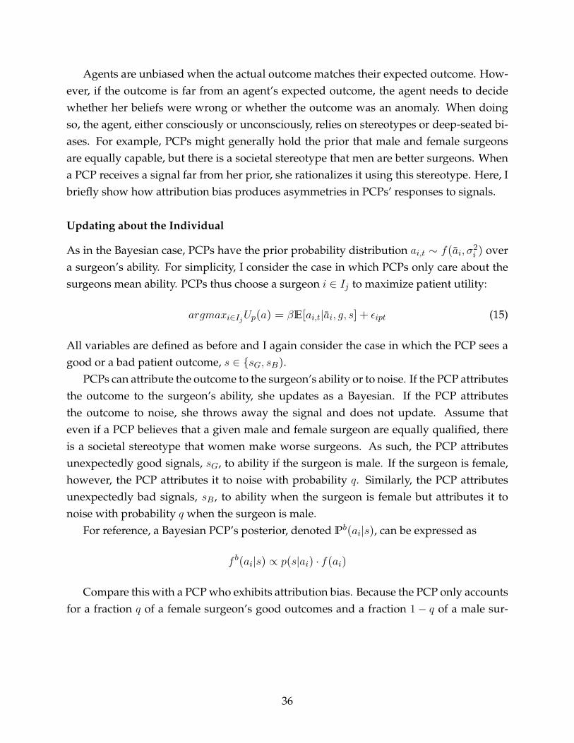
Agents are unbiased when the actual outcome matches their expected outcome. How-ever, if the outcome is far from an agent’s expected outcome, the agent needs to decidewhether her beliefs were wrong or whether the outcome was an anomaly. When doingso, the agent, either consciously or unconsciously, relies on stereotypes or deep-seated bi-ases. For example, PCPs might generally hold the prior that male and female surgeonsare equally capable, but there is a societal stereotype that men are better surgeons. Whena PCP receives a signal far from her prior, she rationalizes it using this stereotype. Here, Ibriefly show how attribution bias produces asymmetries in PCPs’ responses to signals.

Updating about the Individual

As in the Bayesian case, PCPs have the prior probability distribution ai,t ∼ f(ai,σ2i ) over

a surgeon’s ability. For simplicity, I consider the case in which PCPs only care about thesurgeons mean ability. PCPs thus choose a surgeon i ∈ Ij to maximize patient utility:

argmaxi∈IjUp(a) = βE[ai,t|ai, g, s] + εipt (15)

All variables are defined as before and I again consider the case in which the PCP sees agood or a bad patient outcome, s ∈ {sG, sB).

PCPs can attribute the outcome to the surgeon’s ability or to noise. If the PCP attributesthe outcome to the surgeon’s ability, she updates as a Bayesian. If the PCP attributesthe outcome to noise, she throws away the signal and does not update. Assume thateven if a PCP believes that a given male and female surgeon are equally qualified, thereis a societal stereotype that women make worse surgeons. As such, the PCP attributesunexpectedly good signals, sG, to ability if the surgeon is male. If the surgeon is female,however, the PCP attributes it to noise with probability q. Similarly, the PCP attributesunexpectedly bad signals, sB , to ability when the surgeon is female but attributes it tonoise with probability q when the surgeon is male.

For reference, a Bayesian PCP’s posterior, denoted Pb(ai|s), can be expressed as

f b(ai|s) ∝ p(s|ai) · f(ai)

Compare this with a PCP who exhibits attribution bias. Because the PCP only accountsfor a fraction q of a female surgeon’s good outcomes and a fraction 1− q of a male sur-

36

geon’s bad outcomes, her posterior will be distributed

f c(ai|sG) ∝ [1− (1− q) · 1(g = w)] · f b(ai|sG) + (1− q) · 1(g = w)f(ai) (16)

f c(ai|sB) ∝ [1− q · 1(g = m)] · f b(ai|sB) + q · 1(g = m)f(ai) (17)

after a good and bad signal respectively. In the above equations, 1(g = w) is an indicatortaking the value one if the surgeon is female. Similarly, 1(g = m) takes the value onewhen the surgeon is male.

Consider a female surgeon. In equation 16, 1(g = w) = 1 and in equation 17, 1(g =

m) = 0. If a female surgeon sends a good signal, the PCP updates as a Bayesian with prob-ability q and does not update with probability 1− q. In the latter case, the PCP’s beliefs donot change from the prior period. The PCP’s posterior is thus a weighted average of theBayesian posterior and the PCP’s prior. However, if a male surgeon sends a good signal,the PCP updates as a Bayesian. After a bad signal we see the opposite: the PCP updatesas a Bayesian if the surgeon is female and has a posterior that is a weighted average if thesurgeon is male, producing the asymmetries observed in the data.

Updating about the Group

Attribution bias also helps explain the group-level results. PCPs update iteratively aboutgroups after seeing signals from different surgeons. Because women are underrepresentedamong surgeons, PCPs will see fewer patient outcomes under women each quarter evenif they are referring to them at their population share. If the variance of ai is decreasing inthe number of outcomes a PCP sees, the PCPs beliefs will be more diffuse for women thanfor men. That is, σi < σi, leading PCPs to react more strongly to patient outcomes whenthe surgeon is female. However, if PCPs exhibit attribution bias, the distribution aboutwomen’s ability will shift more after bad outcomes than after good outcomes as PCPsattribute female surgeons’ good outcomes to noise with some probability. A PCP’s beliefsabout a group can therefore change, but it will take many more signals than it would ifthe PCP was Bayesian.

8 Conclusion

Gender gaps in hiring, promotion, and pay persist in many industries. This paper identi-fies a mechanism that contributes to these gaps. Using referral volume to proxy for a PCP’sbeliefs about a surgeon’s ability, I show that PCPs exhibit asymmetric updating, loweringtheir referrals more to women than to men after bad outcomes and increasing them more

37

to men than to women after good outcomes. In addition, PCPs use their experience withone woman to infer the ability of other female surgeons. After a bad experience with onefemale surgeon, PCPs become less likely to form new referral connections with women.

The results are consistent with Bayesian updating under specific assumptions on PCPs’priors about surgeon ability. PCPs would have to believe that women are higher abilitythan men or that the variance of men and women’s abilities shrinks differentially follow-ing signals. However the set of priors required do not match the actual distribution ofsurgeon ability. Therefore, although the results are reconcilable with Bayesian updating,they are inconsistent with PCPs having rational expectations. Behavioral models in whichPCPs selectively ignore some signals, such as attribution bias, help to explain the empiri-cal patterns.

Regardless of the model, the results have implications for how we think about employ-ment decisions. Bayesian updating suggests that two individuals of equal ability and whoperform equally well on a set of tasks will be evaluated in the same way. That is, an em-ployer will hold the same posterior about each individual conditional on having the sameprior and seeing the same signal from each. However, if employers exhibit asymmetricupdating, two employees with the same objective performance could end up on differentcareer tracks as the employer treats their performances differently. In this setting, womenare punished for one mistake in the same way that men are punished for three mistakes,leading to lower skill accumulation and pay.

The implications of these results are especially important in occupations where womenare underrepresented. Because employers see relatively few signals from women, the per-formance of one woman spills over to employers’ beliefs about other women. When em-ployers update asymmetrically, they might be too quick to let a woman go after a mistakeand then be unwilling to hire more women in the future, preventing them from learningabout the true distribution of women’s abilities.

38

References

[1] Altonji, Joseph and Charles Pierret. 2001. "Employer Learning and Statistical Discrim-ination." The Quarterly Journal of Economics, 116(1): 313-350.

[2] Antecol, Heather, Kelly Bedard, and Jenna Stearns. 2016. "Equal but Inequitable: WhoBenefits from Gender-Neutral Tenure Clock Stopping Policies?" IZA Discussion PaperNo. 9904.

[3] Arrow, Kenneth. 1973. "The Theory of Discrimination." In Orley Ashenfelter and Al-bert Rees, eds. Discrimination in Labor Markets. Princeton: Princeton UniversityPress.

[4] Azmat, Ghazala and Rosa Ferrer. 2017. "Gender Gaps in Performance: Evidence fromYoung Lawyers." Journal of Political Economy, 125(5): 1306-1355.

[5] Babcock, Linda and Sara Laschever. 2004. Women Don’t Ask. Princeton UniversityPress.

[6] Bagues, Manuel, Mauro Sylos-Labini, and Natalia Zinovyeva. 2017. "Does the GenderComposition of Scientific Committees Matter?" American Economic Review, 107(4):1207-38.

[7] Barber, Brad and Terrance Odean. 2001. "Boys Will be Boys: Gender, Overconfidence,and Common Stock Investment." The Quarterly Journal of Economics, 116(1): 261-292.

[8] Barnett, Michael, Nancy Keating, Nicholas Christakis, James O’Malley, and Bruce Lan-don. 2012a. "Reasons for Choice of Referral Physician Among Primary Care and Spe-cialist Physicians." Journal of General Internal Medicine, 27(5): 506-512.

[9] Barnett, Michael, Ziruir Song, and Brucen Landon. 2012b. "Trends in Physician Refer-rals in the United States, 1999-2009." Archives of Internal Medicine, 172(2): 163-170.

[10] Becker, Gary. 1957. The Economics of Discrimination. Chicago: University of ChicagoPress.

[11] Bertrand, Marianne and Sendhil Mullainathan. 2004. "Are Emily and Greg More Em-ployable than Lakisha and Jamal? A Field Experiment on Labor Market Discrimina-tion." American Economic Review, 94(4): 991-1013.

[12] Beyer, Sylvia. 1990. "Gender Differences in the Accuracy of Self-Evaluations of Per-formance." Journal of Personality and Social Psychology, 59: 960-970.

39

[13] Blau, Francine and Lawrence Kahn. 2016. "The Gender Wage Gap: Extend, Trends,and Explanations." NBER Working Paper No. 21913.

[14] Bordalo, Pedro, Katherine Coffman, Nicola Gennaioli, and Andrei Shleifer. 2016."Stereotypes." The Quarterly Journal of Economics, 131(4): 1753-1794.

[15] Bursztyn, Leonardo, Thomas Fujiwara, and Amanda Pallais. "’Acting Wife’: Mar-riage Market Incentives and Labor Market Investments." American Economic Review,forthcoming.

[16] Casadevall, Arturo and Jo Handelsman. 2014. "The Presence of Female ConvenersCorrelates with a Higher Proportion of Female Speakers at Scientific Symposia." mBio,5(1): e00846-13.

[17] Card, David, Ana Rute Cardoso, and Patrick Kline. 2016. "Bargaining, Sorting, andthe Gender Wage Gap: Quantifying the Impact of Firms on the Relative Pay ofWomen." The Quarterly Journal of Economics, 131(2): 633-686.

[18] Ceci, Stephen, Donna Ginther, Shulamit Kahn, and Wendy Williams. 2014. "Womenin Academic Science: A Changing Landscape." Psychological Science in the PublicInterest, 15(3): 1-67.

[19] Choudhry, Niteesh K., Joshua M. Liao, and Allan S. Detsky. 2014. "Selecting a Spe-cialist: Adding Evidence to the Clinical Practice of Making Referrals." Journal of theAmerican Medical Association, 312(18): 1861-1862.

[20] Coate, Stephen and Glenn Loury. 1993. "Will Affirmative Action Policies EliminateNegative Stereotypes?" American Economic Review, 83(5): 1220-12042.

[21] Eil, David and Justin Rao. 2011. "The Good News-Bad News Effect: Asymmetric Pro-cessing of Objective Information about Yourself." American Economic Journal: Mi-croeconomics, 3(2): 114-38.

[22] Egan, Mark L., Gregor Matvos, and Amit Seru. 2017. “When Harry Fired Sally: TheDouble Standard in Punishing Misconduct.” NBER Working Paper No. 23242.

[23] Farber, Henry and Robert Gibbons. 1996. "Learning and Wage Dynamics." The Quar-terly Journal of Economics, 111(4): 1007-1047.

[24] Freedman, Rachel A., Elena M. Kouri, Dee W. West, and Nancy L. Keating. 2015.“Racial/Ethnic Differences in Patients’ Selection of Surgeons and Hospitals for BreastCancer Surgery.” JAMA Oncology, 1(2): 222-230.

40

[25] Forrest, Christopher, Paul Nutting, Sarah von Schrader, Charles Rohde, and BarbaraStarfield. 2006. "Primary Care Physician Specialty Referral Decision Making: Patient,Physician, and Health Care System Determinants." Medical Decision Making, Jan-Feb.

[26] Fryer, Roland. 2007. "Belief Flipping in a Dynamic Model of Statistical Discrimina-tion." Journal of Public Economics, 91(5-6): 1151-1166.

[27] Fryer, Roland, Philipp Harms, and Matthew Jackson. 2017. "Updating Beliefs whenEvidence is Open to Interpretation: Implications for Bias and Polarization." Workingpaper.

[28] Ginther, Donna and Shulamit Kahn. 2004. “Women in Economics: Moving Up orFalling Off the Academic Career Ladder?” Journal of Economics Perspectives, 18(3):193-214.

[29] Glover, Dylan, Amanda Pallais, and William Pariente. 2017. "Discrimination as a Self-Fulfilling Prophecy: Evidence from French Grocery Stores." The Quarterly Journal ofEconomics, 132(3): 1219-1260.

[30] Goldin, Claudia. 2014a. "A Grand Gender Convergence: Its Last Chapter." AmericanEconomic Review, 104(4): 1091-1119.

[31] Goldin, Claudia. 2014b. "A Pollution Theory of Discrimination: Male and FemaleDifferences in Occupations and Earnings." in L. Boustan, C. Frydman, and R. Margo,Human Capital and History: The American Record (Chicago: University of ChicagoPress), pp. 313-48.

[32] Goldin, Claudia, and Cecilia Rouse. 2000. "Orchestrating Impartiality: The Impact of’Blind’ Auditions on Female Musicians," American Economic Review, 90(4): 715-741.

[33] Gregory, A., R.J. Skiba, and P.A. Noguera. 2010. "The Achievement Gap and the Dis-cipline Gap: Two Sides of the Same Coin?" Educational Researcher, 39: 59-68.

[34] Hughes, Gordon. 1991. "The Learning Curve in Staples Surgery." The Laryngoscope,101(12): 1280-1284.

[35] Jena, Anupam, Andrew Olenski, and Daniel Blumental. 2016. "Sex Differences inPhysician Salary in US Public Medical Schools." JAMA Internal Medicine, 176(9):1294-1304.

41

[36] Kahn, Lisa and Fabian Lange. 2014. "Employer Learning, Productivity, and the Earn-ings Distribution: Evidence from Performance Measures." The Review of EconomicStudies, 81(4): 1575-1613.

[37] Keating, Nancy L., A. James O’Malley, Jukka-Pekka Onnela, and Bruce E. Landon.2017. “Assessing the Impact of Colonoscopy Complications on Use of ColonoscopyAmong Primary Care Physicians and Other Connected Physicians: An ObservationalStudy of Older Americans.” BMJ Open, 7.

[38] Keehner, Madeleine, Yvonne Lippa, Daniel Montello, Frank Tendick, and MaryHegarty. 2006. "Learning a Spatial Skill for Surgery: How the Contributions of Abili-ties Change with Practice." Applied Cognitive Psychology, 20(4): 487-503.

[39] Kinchen, Kraig, Lisa Cooper, David Levine, Nae Yuh Wang, and Neil Powe. 2004."Referral of Patients to Specialists: Factors Affecting Choice of Specialist by PrimaryCare Physicians." Annals of Family Medicine, 2(3): 245-252.

[40] Kleven, Henrik, Camille Landais, and Jakob Egholt Sogaard. 2017. "Children andGender Inequality: Evidence from Denmark." Working paper.

[41] Lautenberger, Diana, Valerie Dandar, Claudia Raezer, and Rae Anne Sloane. 204."The State of Women in Academic Medicine." Association of American Medical Col-leges Annual Report.

[42] Lichtenstein, S., B. Fischhoff, and L.D. Phillips. 1982. Calibration of probabilities: Thestate of the art to 1980. In D. Kahneman, P. Slovic, & A. Tversky (Eds.), Judgementunder uncertainty: Heuristics and biases, (pp. 306-334). Cambridge, England: Cam-bridge University Press.

[43] Lo Sasso, Anthony, Michael Richards, Chiu-Fang Chou, and Susan Gerber. 2011. "The$16,819 Pay Gap for Newly Trained Physicians: The Unexplained Trend of Men Earn-ing More Than Women." Health Affairs, 30(2): 193-201.

[44] Ly, Dan, Seth Seabury, and Anupam Jena. 2016. "Differences in Incomes of Physiciansin the United States by Race and Sex: Observational Study." BMJ, 353: i2921.

[45] Medscape Physician Compensation Report. 2017. Sarah Grisham, Senior Edi-tor. Art Science Code LLC. <http://www.medscape.com/slideshow/compensation-2017-overview-6008547>

42

[46] Mobius, Markus, Muriel Niederle, Paul Niehaus, and Tanya Rosenblat. 2015. "Man-aging Self-Confidence." Working paper.

[47] Niederle, Muriel and Lise Vesterlund. 2007. "Do Women Shy Away From Competi-tion? Do Men Compete Too Much?" Quarterly Journal of Economics, 122(3): 1067-1101.

[48] Noonan, Mary, Mary Corcoran, and Paul Courant. 2005. "Pay Differences Amongthe Highly Trained: Cohort Differences in hte Sex Gap in Lawyers’ Earnings." SocialForces, 84(2): 851-870.

[49] Phelps, Edmond. "The Statistical Theory of Racism and Sexism." American EconomicReview, 62(4): 659-661.

[50] Pinkston, Joshua. 2009. "A Model of Asymmetric Employer Learning with TestableImplications." The Review of Economic Studies, 76(1): 367-394.

[51] Rabin, Matthew and Joel Schragg. 1999. "First Impressions Matter: A Model of Con-firmatory Bias." Quarterly Journal of Economics, 114(1): 37-82.

[52] Sasser, Alicia. 2005. "Gender Differences in Physician Pay: Tradeoffs Between Careerand Family." The Journal of Human Resources, 40(2): 477-504.

[53] Shea, Dennis, Bruce Stuart, Joseph Vasey, and Soma Ng. 1999. "Medicare PhysicianReferral Patterns." Health Services Research, 34(1): 331-348.

[54] Skiba, Russell J., Robert S. Michael, Abra Carroll Nardo, and Reece L. Peterson. 2002.“The Color of Discipline: Sources of Racial and Gender Disproportionality in SchoolPunishment.” The Urban Review, 34(3): 317-342.

[55] Zeltzer, Dan. 2017. "Gender Homophily in Referral Networks: Consequencesfor the Medicare Physician Earnings Gap." Working paper. Available at SSRN:https://ssrn.com/abstract=2921482

43

Figures

FIGURE 1: GENDER BREAKDOWN OF SPECIALTIES

Notes: This figure displays the surgical specialties that could be included in the analysis (i.e. the specialties available to match on) andthe gender composition of each. The gender distributions are calculated using the number of surgeons represented in each specialtyin the Medicare dataset and therefore may be slightly different than the gender distribution when including all surgeons (such asthose not accepting Medicare). Int. Cardiology is Internal Cardiology and Int. Pain Management is Internal Pain Management.

44

FIGURE 2: DISTRIBUTION OF SURGEON ABILITY

(a) Ability PDF

(b) Ability CDF

Notes: This figure shows the distributions of male and female surgeon ability, where ability is defined as the difference between apatient’s risk of death for the given procedure and an indicator variable that equals one if the patient died, averaged over all of asurgeon’s patients. The top figure is the PDF and the bottom figure is the CDF. The full sample of surgical specialists is used to createthese distributions.

45

FIGURE 3: QUARTERLY ESTIMATES OF PCP’S REACTION TO DEATH

Notes: This figure plots the quarterly regression coefficients and 95% confidence intervals from estimating equation 3 using the sampleof matched male and female surgeons who experience a patient death. The coefficients are plotted relative to the number of referralsthe surgeon was receiving from the PCP in k = −1, which are normalized to zero. In k = −1, male and female surgeons bothreceived an average of 0.65 referrals from PCP j. A patient that PCP j referred to surgeon i dies in k = 0. The outcome variable is thetotal number of referrals that PCP j sends to surgeon i each quarter. Standard errors are clustered at the PCP-surgeon match level.

46

FIGURE 4: COMPARISON WITH PLACEBO SURGEONS

(a) Male Surgeons (b) Female Surgeons

(c) Difference-in-Differences

Notes: This figure shows three plots that compare the impact of a bad event to “placebo” outcomes. Panels (a) and (b) plot thequarterly regression coefficients and 95% confidence intervals from estimating equation 4 on the matched sample of male (panel a)and female (panel b) surgeons who did not experience a patient death. In each panel, PCP j refers a patient to surgeon i and thesurgery does not result in a patient death. I then plot the quarterly coefficients from Figure 3. Panel (c) shows difference-in-differencesestimates and 95% confidence intervals. The estimates show the difference between referrals to a female and a male surgeon in quarterk. The grey circles show the estimates for the sample of placebo surgeons and the green triangles show the estimates for the sample ofmatched surgeons who experience a patient death. All coefficients are plotted relative to the number of referrals the surgeon wasreceiving from the PCP in k = −1, which are normalized to zero. Standard errors are clustered at the PCP-surgeon match level.

47

FIGURE 5: RISKINESS OF FUTURE PROCEDURES AND PATIENTS

(a) Patient Risk

(b) Procedure Risk

Notes: Panels A and B show how the riskiness of future patients and procedures change after a patient death. The outcome variable inPanel A is the average patient risk of the patients that PCP j sends to surgeon i in quarter t, excluding the risk level of the patient whodied. The outcome variable in Panel B is the average death rate of the procedures that PCP j sends to surgeon i in quarter t, againexcluding the riskiness of the procedure that the patient who died was referred for. The coefficients are plotted relative to the averagepatient risk or procedure death rate that the surgeon received in k = −1, which is normalized to zero. Standard errors are clustered atthe PCP-surgeon match level. See Section 2 for the definition and calculation of patient risk.

48

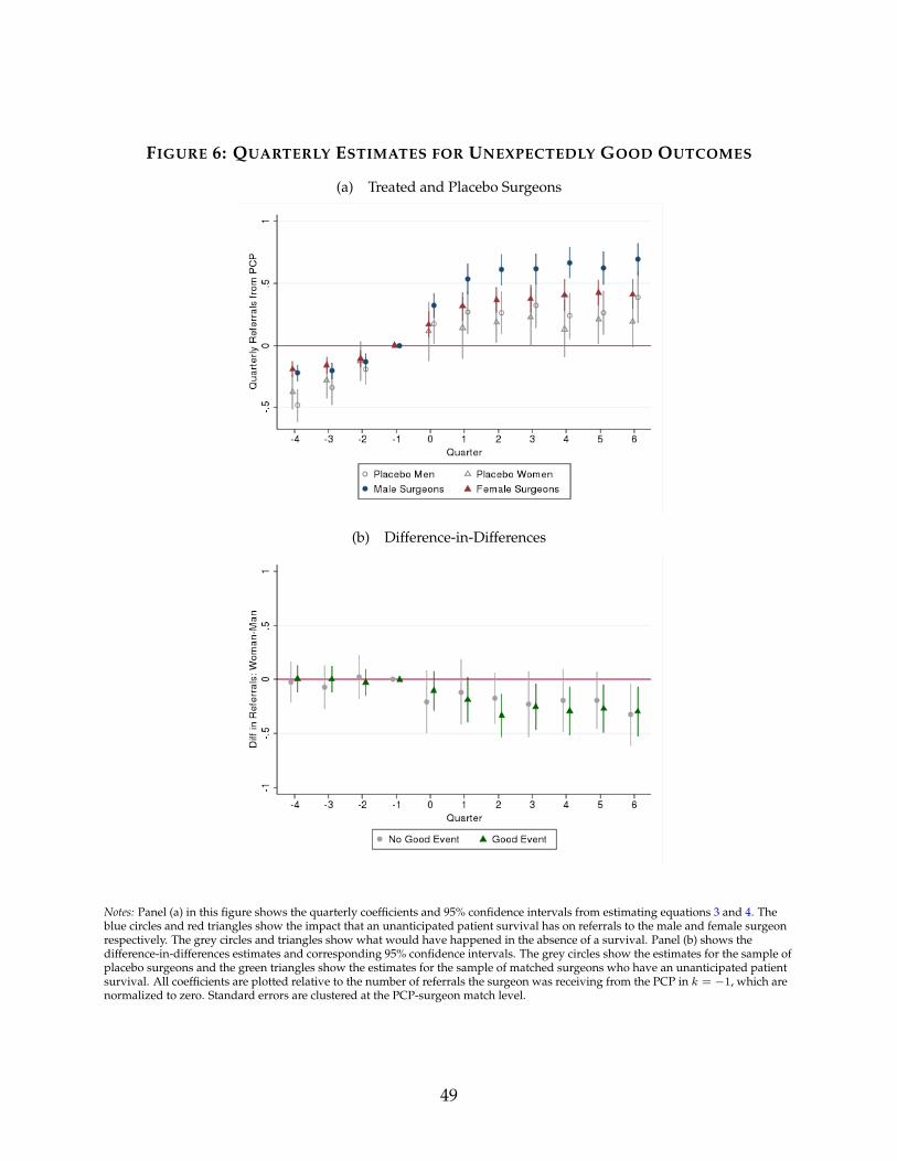
FIGURE 6: QUARTERLY ESTIMATES FOR UNEXPECTEDLY GOOD OUTCOMES

(a) Treated and Placebo Surgeons

(b) Difference-in-Differences

Notes: Panel (a) in this figure shows the quarterly coefficients and 95% confidence intervals from estimating equations 3 and 4. Theblue circles and red triangles show the impact that an unanticipated patient survival has on referrals to the male and female surgeonrespectively. The grey circles and triangles show what would have happened in the absence of a survival. Panel (b) shows thedifference-in-differences estimates and corresponding 95% confidence intervals. The grey circles show the estimates for the sample ofplacebo surgeons and the green triangles show the estimates for the sample of matched surgeons who have an unanticipated patientsurvival. All coefficients are plotted relative to the number of referrals the surgeon was receiving from the PCP in k = −1, which arenormalized to zero. Standard errors are clustered at the PCP-surgeon match level.

49

FIGURE 7: SPILLOVERS TO OTHER SURGEONS AFTER BAD OUTCOME

Notes: This figure shows how PCPs change their behaviour toward other surgeons after a patient death. In k = 0, a patient that PCP jsent to surgeon i dies. The outcome variable is the fraction of new referrals going to female or male surgeons (whom PCP j hasn’treferred to before), excluding the performing surgeon. Specifically, the blue circles are estimated from a regression using the fractionof referrals going to men as the outcome and the red triangles are estimated from a regression using the fraction of referrals going towomen as the outcome. The coefficients are plotted relative to the number of referrals that PCP j was sending to surgeons she had notpreviously referred to in quarter k = −1. I control for the fraction of available surgeon who are male or female and also includePCP-surgeon match fixed effects. Standard errors are clustered at the PCP-surgeon match level.

50

FIGURE 8: INFORMATION SPILLOVERS TO OTHER PCPS

(a) Referrals from PCPs in Group Practice

(b) Referrals from PCPs Outside of Practice

Notes: This figure shows how referrals from other PCPs to a performing surgeon change after a bad event.The outcome variable in Panel (a) is the number of quarterly referrals from PCPs in the referring PCP’sgroup practice. Group practices are restricted to those with less than 20 members for reasons outlined inSection 4. The outcome variable in Panel (b) is the number of quarterly referrals from PCPs outside of thereferring PCP’s group practice but in the same Hospital Referral Region. Both panels are estimated on thesample of matched male and female surgeons who experience a patient death. All coefficients are plottedrelative to the number of referrals the surgeon was receiving from the PCP in k = −1, which arenormalized to zero. Standard errors are clustered at the PCP-surgeon match level.

51

FIGURE 9: PCP RESPONSE BY PATIENT RISK

Notes: This binned scatterplot shows the relationship between the risk of the patient that died and the change in referrals from PCP jto surgeon i, using the matched sample of male and female surgeons who experience a patient death. Patient risk is calculated as inSection 2 and is then binned into deciles. Both variables are residualized on a PCP-surgeon match pair effect. The line of best fit usingOLS is shown separately for male and female surgeons. The lines of best fit have slopes of 0.060 (s.e. = 0.004) for female surgeon and0.026 (s.e. = 0.002) for male surgeons.

FIGURE 10: CHANGE IN SURGEON QUALITY

Notes: This figure shows how the quality of surgeon that a PCP refers to changes after a patient death. In the figure, a patient thatsurgeon i received from PCP j dies in quarter k = 0. The outcome variable is the standard deviation of surgeon ability from themean. The coefficients are plotted relative to the standard deviation of surgeon quality that the PCP was referring to in k = −1. Forexample, if a PCP was referring to surgeons who were an average of 1 standard deviation above the mean in k = −1, all coefficientsare plotted relative to 1. Standard errors are clustered at the PCP level.

52

FIGURE 11: MEDICARE PAYMENTS

Notes: This figure shows plots quarterly Medicare payments using the sample of matched surgeons who experience a patient death.The outcome variable is the total quarterly Medicare payments that surgeon i received from j’s referrals. The coefficients are plottedrelative to the total Medicare payments that the surgeon was receiving from the PCP in k = −1. Payments in k = −1 are normalizedto zero. A patient that PCP j referred to surgeon i dies in k = 0. Standard errors are clustered at the PCP-surgeon match level.

53

Tables

TABLE 1: SUMMARY STATISTICS: UNMATCHED SAMPLE

Male Surgeons Female SurgeonsMean SD Mean SD p-value

Panel A: SurgeonsTotal Patients 112.4 170.0 81.2 144.1 0.001

Freq. of Bad Events (%) 0.85 4.4 0.72 4.3 0.001Freq. of Good Events (%) 26.0 27.0 26.1 26.0 0.013# PCPs Referring 18.6. 27.1 14.7 25.2 0.001Patient Risk (%) 0.48 0.35 0.40 0.33 0.001Patient Female (%) 52.9 30.0 58.5 32.5 0.001Patient Minority (%) 17.6 25.4 18.5 28.0 0.001Patient Age 71.8 8.3 70.8 9.7 0.001Surgeon Ability 0.0011 0.0053 0.0012 0.0052 0.001

Observations 152,237 30,603Panel B: Primary Care Physicians Male Surgeons Female Surgeons

Mean SD Mean SD p-value# Surgeons Referred To 15.5 13.2 2.5 3.2 0.001# Surgeons Referred to for a Proc. 1.41 1.24 0.17 0.51 0.001

Observations 181,237 50,603

Notes: This table shows summary statistics for the full sample of surgeons. The variables are measuredat the yearly so that Total Patients is the average number of patients a surgeon receives in a year, forexample. Total Events is the number of good and bad events a surgeon experiences and # of PCPsReferring is the average number of PCPs that a given surgeon receives referrals from in a year. PatientRisk and Surgeon Ability are calculated as in Section 2

54

TABLE 2: BALANCE TABLE: MATCHED SAMPLE FOR BAD OUTCOMES

Male Surgeons Female SurgeonsMean SD Mean SD p-value

Patient Refs from PCP 24.9 33.7 25.2 34.3 0.639Frac. of PCP’s Refs for Proc. 50.6 14.0 50.7 14.1 0.454Total Patient Refs (Any PCP) 74.2 116.5 73.4 115.2 0.651Patient Age 77.2 12.0 77.2 12.1 0.887Patient Minority (%) 8.4 27.7 8.4 27.7 0.999Patient Female (%) 49.6 50.0 49.6 50.0 0.999Patient Risk (%) 0.81 0.40 0.81 0.40 0.915Risk All Past Ptnts 0.007 0.004 0.007 0.004 0.830Total Procs. Performed 10.5 15.5 10.6 15.5 0.593Years of Experience 23.3 8.1 23.2 8.0 0.174Available Surgeons 44.5 27.8 45.1 27.8 0.137# of Matched Surgeons 7,757 7,757# Unique Surgeons 5,579 3,561

Notes: The balance table shows summary statistics for the matched sample of surgeons whoexperience a death. The sample is matched exactly on patient gender and minority status aswell as surgeon specialty and procedure (not shown above). The sample is matched coarselyon all other variables. Patient Refs from PCP and Frac. of PCP’s Refs for Proc are the numberand fraction of referrals that surgeon i received from PCP j in quarters t = −5 through t = −2where patient p dies in t = 0. Similarly, Total Patients Refs is the number of patients surgeon ireceived from any PCP during this period. Patient Risk is the risk level of the patient who dieswhile Risk All Past Ptnts is the average risk of all past patients surgeon i received betweent = −5 and t = −2. Total Procs. Performed is the number times surgeon i performed theprocedure that PCP j refers for between t = −5 and t = −2. Years of Experience is thenumber of years since the surgeon graduated from medical school. Available Surgeons is thenumber of surgeons who are in the same specialty as surgeon i that the referring PCP has theoption of referring to. This is measured using Hospital Referral Region as the geographicalunit.

55

TABLE 3: BALANCE TABLE: MATCHED SAMPLE FOR GOOD OUTCOMES

Male Surgeons Female SurgeonsMean SD Mean SD p-value

Patient Refs from PCP 15.5 21.0 15.5 21.0 0.481Frac. of PCP’s Refs for Proc (%) 34.2 7.3 34.1 7.1 0.835Total Patient Refs (Any PCP) 45.5 68.5 45.0 68.0 0.645Patient Age 91.3 4.7 91.3 4.6 0.353Patient Minority (%) 4.8 21.3 4.8 21.3 0.999Patient Female (%) 24.6 43.1 24.6 43.1 0.999Patient Risk 0.017 0.002 0.017 0.002 0.650Risk All Past Ptnts 0.015 0.004 0.015 0.004 0.850Total Procs. Performed 8.0 15.5 8.0 15.3 0.861Years of Experience 22.9 8.4 22.7 8.5 0.461Available Surgeons 38.9 25.9 38.7 25.7 0.603# Matched Surgeons 6,979 6,979# Unique Surgeons 5,554 2,882

Notes: The balance table shows summary statistics for the matched sample of surgeons whoexperience an “unexpectedly good” outcome. The sample is matched exactly on patient genderand minority status as well as surgeon specialty and procedure (not shown above). The sampleis matched coarsely on all other variables. Patient Refs from PCP and Frac. of PCP’s Refs for Procare the number and fraction of referrals that surgeon i received from PCP j in quarters t = −5through t = −2 where patient p dies in t = 0. Similarly, Total Patients Refs is the number ofpatients surgeon i received from any PCP during this period. Patient Risk is the risk level ofthe patient who dies while Risk All Past Ptnts is the average risk of all past patients surgeon ireceived between t = −5 and t = −2. Total Procs. Performed is the number times surgeon iperformed the procedure that PCP j refers for between t = −5 and t = −2. Years of Experienceis the number of years since the surgeon graduated from medical school. Available Surgeons isthe number of surgeons who are in the same specialty as surgeon i that the referring PCP has theoption of referring to. This is measured using Hospital Referral Region as the geographical unit.

56

TABLE 4: IMPACT OF EVENT ON REFERRALS TO PERFORMING SURGEON

Referrals Medicare Pay ($)(1) (2) (3) (4)

Event Bad Good Bad GoodPost 0.006 0.509∗∗∗ -80.05∗∗∗ 145.29∗∗∗

(0.058) (0.069) (25.09) (45.21)Female × Post -0.291∗∗∗ -0.222∗∗ -138.97∗∗∗ -22.88

(0.087) (0.100) (32.54) (64.14)Time Trend 0.099∗∗∗ 0.073∗∗∗ 31.84∗∗∗ 27.58∗∗∗

(0.011) (0.011) (5.84) (8.07)Female × Time Trend -0.009 -0.010 13.67∗∗∗ -6.08

(0.013) (0.015) (4.65) (8.59)Post × Time Trend -0.072∗∗∗ -0.046∗∗∗ -35.51∗∗∗ -41.83∗∗∗

(0.012) (0.012) (6.00) (8.82)Average Post Effect On:

Male Surgeons 0.101 0.604 -92.90 95.42Female Surgeons -0.222 0.346 -184.02 51.26

Mean of Outcome Var. 0.65 0.48 309.17 264.86Observations 34,053 29,214 34,053 29,214Clusters 3,425 2,948 3,425 2,948R-Squared 0.265 0.325 0.237 0.249

Notes: This table displays the effect of a bad event (columns 1 and 3) and a good event(columns 2 and 3) on referrals and Medicare payments to the performing surgeon. Incolumns 1 and 2, the outcome variable the number of referrals from the referring PCP tothe performing surgeon in a quarter. In columns 3 and, the outcome variable is the to-tal Medicare pay that the surgeon receives from referrals from the PCP. All regression in-clude surgeon-PCP match fixed effects and standard errors are clustered at the surgeon-PCPmatch level. Columns 1 and 3 are estimated on the sample of matched male and female sur-geons who experience a patient death. Columns 2 and 4 are estimated on the sample ofmatched male and female surgeons who experience a good patient outcome. Both samplesare limited to PCP-surgeon pairs in which the PCP had referred between 1 and 10 patientsin the past. PCP-surgeon match fixed effects are included in all regressions and standarderrors are clustered at the PCP-surgeon match level. Levels of significance: *10%, ** 5%, and*** 1% level.

57

TABLE 5: IMPACT OF AN EVENT ON REFERRALS TO OTHERS

Fraction of New Referrals to Women in: Same Specialty Other Specialty(1) (2) (3)

Event Bad Good BadPost 0.011 -0.022 0.007

(0.025) (0.028) (0.012)Female × Post -0.097∗∗ 0.034 -0.028

(0.039) (0.044) (0.018)Time Trend 0.003 0.003 0.004

(0.006) (0.008) (0.003)Female × Time Trend -0.003 0.002 0.001

(0.010) (0.012) (0.004)Post × Time Trend -0.004 -0.001 -0.005

(0.007) (0.009) (0.004)Female × Post × Time Trend 0.006 0.001 -0.001

(0.012) (0.014) (0.005)Avg. Post Effect -0.079 0.029 -0.025Mean of Outcome Var. 0.15 0.12 0.13Observations 34,053 29,214 34,053Clusters 3,425 2,948 3,425R-Squared 0.417 0.350 0.206

Notes: This table displays the effect of a bad (columns 1 and 3) or a good (column 2) event by aperforming surgeon on referrals to other surgeons of the same gender. The outcome variable isthe fraction of a PCP’s new referrals that go to men or women, excluding the performing surgeon.Columns 1 and 2 look at the fraction of new referrals going to women/men in the same specialty asthe performing surgeon while Column 3 looks at the fraction of new referrals going to women/menin other specialties. I control for the fraction of available of surgeons who are women or menwithin the same specialty (Columns 1 and 2) or in any specialty (Columns 3). Regressions areestimated using the sample of matched male and female surgeons who experience a patient deathor an unexpectedly good outcome. Levels of significance: *10%, ** 5%, and *** 1% level.

58

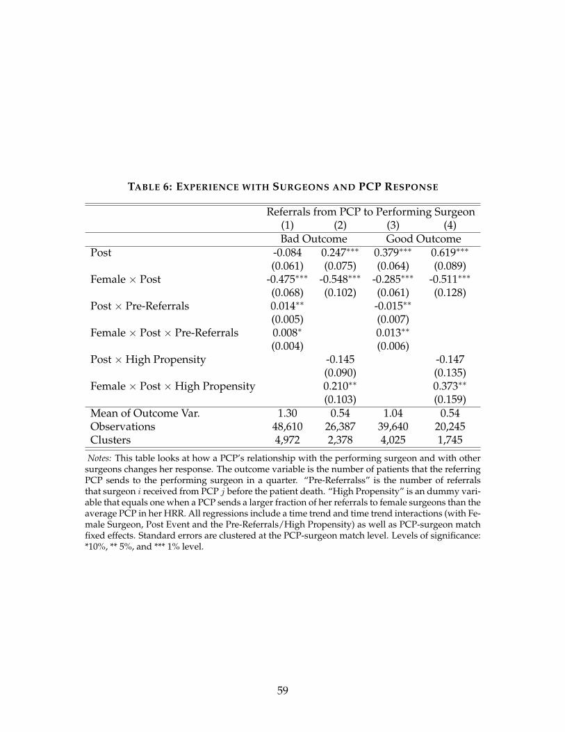
TABLE 6: EXPERIENCE WITH SURGEONS AND PCP RESPONSE

Referrals from PCP to Performing Surgeon(1) (2) (3) (4)Bad Outcome Good Outcome

Post -0.084 0.247∗∗∗ 0.379∗∗∗ 0.619∗∗∗

(0.061) (0.075) (0.064) (0.089)Female × Post -0.475∗∗∗ -0.548∗∗∗ -0.285∗∗∗ -0.511∗∗∗

(0.068) (0.102) (0.061) (0.128)Post × Pre-Referrals 0.014∗∗ -0.015∗∗

(0.005) (0.007)Female × Post × Pre-Referrals 0.008∗ 0.013∗∗

(0.004) (0.006)Post × High Propensity -0.145 -0.147

(0.090) (0.135)Female × Post × High Propensity 0.210∗∗ 0.373∗∗

(0.103) (0.159)Mean of Outcome Var. 1.30 0.54 1.04 0.54Observations 48,610 26,387 39,640 20,245Clusters 4,972 2,378 4,025 1,745

Notes: This table looks at how a PCP’s relationship with the performing surgeon and with othersurgeons changes her response. The outcome variable is the number of patients that the referringPCP sends to the performing surgeon in a quarter. “Pre-Referralss” is the number of referralsthat surgeon i received from PCP j before the patient death. “High Propensity” is an dummy vari-able that equals one when a PCP sends a larger fraction of her referrals to female surgeons than theaverage PCP in her HRR. All regressions include a time trend and time trend interactions (with Fe-male Surgeon, Post Event and the Pre-Referrals/High Propensity) as well as PCP-surgeon matchfixed effects. Standard errors are clustered at the PCP-surgeon match level. Levels of significance:*10%, ** 5%, and *** 1% level.

59

TABLE 7: VARIABLES CORRELATED WITH SURGEON RESPONSE

Referrals to SurgeonX-Var: Num. Surgeons Surgeon Exp. PCP Exp. Female PCP

(1) (2) (3) (4)Post -0.256∗ -0.043 0.177 0.109

(0.129) (0.131) (0.160) (0.058)Female × Post -0.522∗∗∗ -0.306∗∗ -0.518∗∗ -0.434∗∗∗

(0.119) (0.130) (0.199) (0.056)Post × X-Var 0.004 0.002 -0.004 0.058

(0.002) (0.006) (0.006) (0.140)Female × Post × X-Var 0.004 0.003 0.008 0.185

(0.002) (0.010) (0.008) (0.123)Observations 17,691 34,054 28,989 28,989Clusters 1,781 2,945 2,578 2,914

Notes: This table tests whether the four variables listed at the top of each column are correlated with aPCP’s response. Each variable is interacted with the Post and Post×Female variables. “Num. Surgeons” isthe number of surgeons in the same specialty as the performing surgeon who work in the PCP’s HospitalReferral Region (i.e. the PCP’s outside options). “Surgeon Exp.” and “PCP Exp/” are the surgeon andPCP’s experience, measured as the number of years that each doctor has been out of medical school. “PCPFemale” is a dummy variable indicating that the PCP is a woman. A time trend, time trend interactionswith all variables, and a PCP-surgeon match fixed effect are included in each regression. Columns 2 and3 also include surgeon experience squared and PCP experience squared respectively. Standard errors areclustered at the PCP-surgeon match level. Levels of significance: *10%, ** 5%, and *** 1% level.

60

TABLE 8: ARE EVENTS PREDICTIVE OF FUTURE EVENTS?

# Bad Events Any Bad Event # Good Events(1) (2) (3)

Female Surgeon -0.792∗∗ -0.031∗∗∗ -0.045(0.366) (0.011) (0.177)

Log Future Ptnt Risk 0.283 0.223∗∗∗ 0.859∗∗

(0.197) (0.017) (0.321)Future Referrals 0.006∗∗∗ 0.001∗∗ 0.005∗∗∗

(0.001) (0.001) (0.001)Log Past Ptnt Risk -1.173∗∗∗ -0.038∗∗∗ 0.243∗∗∗

(0.380) (0.005) (0.070)Past Referrals -0.001∗ 0.001∗∗∗ -0.002∗∗∗

(0.001) (0.000) (0.000)Surgeon Experience 0.001 -0.001 0.012∗∗∗

(0.013) (0.001) (0.004)Observations 24,459 24,459 24,478R-Squared 0.594 0.373 0.418

Notes: This table shows the results from testing whether events are differentially pre-dictive of future events for male and female surgeons. The sample consists of the fullsample of surgeons who every experienced a bad or good event. Log Future PatientRisk is the average risk of the future patients. Future Referrals is the number of referralsthat the surgeon receives from any PCP in the future. Similarly, # Past Referrals and LogPatient Past Risk are the number of referrals and average risk of those patients that thesurgeon received before the patient death. Surgeon specialty fixed effects are also in-cluded. Standard errors are clustered at the specialty level. Levels of significance: *10%,** 5%, and *** 1% level.

61

Appendix A Data Appendix

A.1 Example of Procedure Code Groupings

Parent Group: Surgical Procedures on the Cardiovascular System

• Surgical Procedures on the Heart and Pericardium

– Surgical Procedures on the Pericardium

– Excision Procedures of Cardiac Tumor

– Transmyocardial Revascularization Procedures

– Pacemaker or Pacing Cardioverter-Defibrillator Procedures

– Electrophysiologic Operative Procedures on the Heart and Pericardium

– Introduction or Removal of Patient-activated Cardiac Event Recorder

– Surgical Procedures on the Heart (Including Valves) and Great Vessels

– Surgical Procedures on Cardiac Valves

∗ Surgical Procedures on the Aortic Valve (22 procedures)

∗ Surgical Procedures on the Mitral Valve (8 procedures)

∗ Surgical Procedures on the Tricuspid Valve (5 procedures)

∗ Surgical Procedures on the Pulmonary Valve (7 procedures)

– Other Cardiac Valvular Procedures

– Coronary Artery Anomaly Procedures

– Endoscopy Procedures on the Heart and Pericardium

– Venous Grafting Only for Coronary Artery Bypass

– Combined Arterial-Venous Grafting for Coronary Bypass

– Arterial Grafting for Coronary Artery Bypass

– Coronary Endarterectomy Procedures

– Repair Procedures for Single Ventricle and Other Complex Cardiac Anomalies

– Repair Procedures for Septal Defect

– Repair Procedures for the Sinus of Valsalva

– Repair Procedures for Venous Anomalies

– Shunting Procedures on the Heart and Pericardium

62

– Repair Procedures for Transposition of the Great Vessels

– Repair Procedures for Truncus Arteriosus

– Repair Procedures for Aortic Anomalies

– Repair Procedures for Thoracic Aortic Aneurysm

– Endovascular Repair Procedures of the Descending Thoracic Aorta

– Surgical Procedures on the Pulmonary Artery

– Heart/Lung Transplantation Procedures

– Extracorporeal Membrane Oxygenation or Extracorporeal Life Support Servicesand Procedures

– Cardiac Assist Procedures

– Other Cardiac Surgery Procedures

• Surgical Procedures on the Arteries and Veins

A.2 Specialties included in matched sample

Cardiac surgery/cardiology, emergency medicine, general surgery, interventional cardi-ology, interventional radiology, nephrology, neurosurgery, orthopedic surgery, otolaryn-gology, plastic and reconstructive surgery, pulmonary disease, surgical oncology, urology,vascular surgery.

Appendix B Appendix to Theoretical Framework

B.1 Calculation of Work Hours Adjustment

Primarily due to fewer work hours, women see approximately 0.67 patients for everypatient a man sees (Medscape Physician Compensation Report, 2016). In the Medicaredata, female surgeons receive 10% of referrals, meaning that they receive 0.1 referralswhen working 2/3 of a “man day” (number of hours men work on average). If we increasea woman’s work hours to be equivalent to a man’s, women should receive 0.05 additionalreferrals (since they receive 0.1 referrals per 2/3 day worked, they receive 0.05 referralsper 1/3 day worked).

Women should thus receive 15% of total referrals.

63

B.2 Proofs

Proof of Proposition 1

Assume that statements 1 and 2 in Proposition 1 hold and that P(sG|w)P(sG|m)

. Statement 2 saysthat

aw − am > E(a|sG,w)−E(a|sG,m) (18)

aw − am > E(a|sB,w)−E(a|sB,m) (19)

Multiplying equations 18 and 19 by P(sG|w) and adding the two inequalities togethergives

P(sG|w)(aw − am) + P(sB|w)(aw − am) >

P(sG|w)(E(a|sG,w)−E(a|sG,m)) + P(sB|w)(E(a|sB,w)−E(a|sB,m))

We then have

aw − am > P(sG|w)(E(a|sG,w)−E(a|sG,m)) + P(sB|w)(E(a|sB,w)−E(a|sB,m))

aw − am > P(sG|w)E(a|sG,w) + P(sB|w)E(a|sB,w) + P(sG|w)E(a|sG,m) + P(sB|w)E(a|sB,m)

aw − am > aw −P(sG|w)E(a|sG,m)−P(sB|w)E(a|sB,m)

am < P(sG|w)E(a|sG,m) + P(sB|w)E(a|sB,m)

(20)

where the law of iterated expectations is used in lines 3-4. Substituting in for am, usingthe fact that P(sB|m) = 1−P(sG|m), and rearranging gives

P(G|m)E(a|sG,m) + P(sB|m)E(a|sB,m) < P(sG|w)E(a|sG,m) + P(sB|w)E(a|sB,m)

P(sG|m)E(a|sG,m) + (1−P(sG|m))E(a|sB,m) < P(sG|w)E(a|sG,m) + (1−P(sG|w))E(a|sB,m)

P(sG|m) · (E(a|sG,m)−E(a|sB,m)) < P(sG|w) · (E(a|sG,m)−E(a|sB,m))

(P(sG|m)−P(sG|w)) · (E(a|sG,m)−E(a|sB,m)) < 0 (21)

For equation 21 to be negative, one of the terms must be negative and the other positive.Note that (E(a|sG,m)−E(a|sB,m)) must be positive by the definition of a good and badevent, so it must be that P(aG|m) < P(aG|w) which violates our initial assumption thatP(sG|w)P(sG|m)

. Thus, if the prior distributions for men and women have the same variance, it

64

must be that the prior on women is higher than the prior on men

Proof of Proposition 2

Assume without loss of generality that the variance over priors is larger for female sur-geons than male surgeons: σ2

w > σ2m. The law of total variance states that the prior vari-

ance is the sum of the variance of the posterior and the (expected) posterior variance:

σ2g = V ar(E[a|s, g]) + E[σ2

g |s]

Taking the difference in the variance of the prior between men and women gives

σ2w − σ2

m = E[σw|s]−E[σm|s] + V ar(E[a|s,w])− V ar(E[a|s,m]) (22)

We have assumed that σ2w − σ2

m > E[σw|s]−E[σm|s]. Substituting 22 into this inequality,we get

E[σw|s]−E[σm|s] + V ar(E[a|s,w])−V ar(E[a|s,m])

> E[σw|s]−E[σm|s]

V ar(E[a|s,w])− V ar(E[a|s,m]) > 0 (23)

Equation final shows that the spread over beliefs about a female surgeon after a signal islarger than the spread in beliefs about a male surgeon after the equivalent signal, meaningthat the PCP must have updated more about the female surgeon after both good and badsignals.

65

Appendix C Additional Tables

TABLE A1: BALANCE FOR PLACEBO MATCHED SAMPLES

Panel A: Male Surgeons No Death DeathMean SD Mean SD p-value

Patient Refs from PCP 25.6 33.4 25.4 34.2 0.654Total Patient Refs 69.3 106.0 69.0 105.9 0.899Patient Age 77.8 9.0 77.9 9.1 0.451Patient Minority (%) 6.8 25.2 6.8 25.2 0.999Patient Female (%) 59.0 49.2 59.0 49.2 0.999Patient Risk (%) 0.85 0.34 0.85 0.35 0.156Risk All Past Ptnts 0.010 0.007 0.010 0.006 0.194Experience (Yrs) 24.9 10.4 24.9 10.3 0.997Available Surgeons 48.7 29.7 49.0 29.6 0.123Observations 15,012 15,012

Panel B: Female Surgeons No Death DeathMean SD Mean SD p-value

Patient Refs from PCP 25.4 44.4 25.1 44.2 0.664Total Patients Refs 72.3 110.0 72.0 107.7 0.821Patient Age 79.7 9.8 79.8 9.8 0.317Patient Minority (%) 5.7 23.2 5.7 23.2 0.999Patient Female (%) 61.2 48.7 61.2 48.7 0.999Patient Risk (%) 0.010 0.004 0.010 0.005 0.162Risk All Past Ptnts 0.009 0.004 0.009 0.004 0.284Experience (Yrs) 22.2 8.3 22.2 8.5 0.640Available Surgeons 48.8 29.7 48.7 29.4 0.254Observations 4,658 4,658

Notes: This balance table shows summary statistics for the matched sample ofsurgeons who did and did not experience a patient death. The surgeons whodid not experience a death are called “placebos” in the paper. To create eachsample, I take the set of male or female surgeons who ever experienced a badevent and match the male surgeons to other men who did not experience a death,and match the female surgeons to other women who did not experience a death.The sample is matched exactly on patient gender and minority status as wellas surgeon specialty and procedure (not shown above). The sample is matchedcoarsely on all other variables. All variables are defined as in Table 2.

66

Appendix D Additional Figures

FIGURE A1: SPILLOVERS TO FEMALE SURGEONS, >10 PRIOR REFS

Notes: This figure shows how PCPs change their behaviour toward other female surgeons after a patient death. In k = 0, a patientthat PCP j sent to surgeon i dies. The outcome variable is the fraction ofreferrals going to female surgeon whom PCP j had referred atleast 10 patients to prior to the death. The estimation is done on the sample of female surgeons who experience a patient death. Thecoefficients are plotted relative to the fraction of referrals that PCPj was sending to these surgeons in quarter k = −1. I control for thefraction of available surgeon who are male or female and also include PCP-surgeon match fixed effects. Standard errors are clusteredat the PCP-surgeon match level.

67

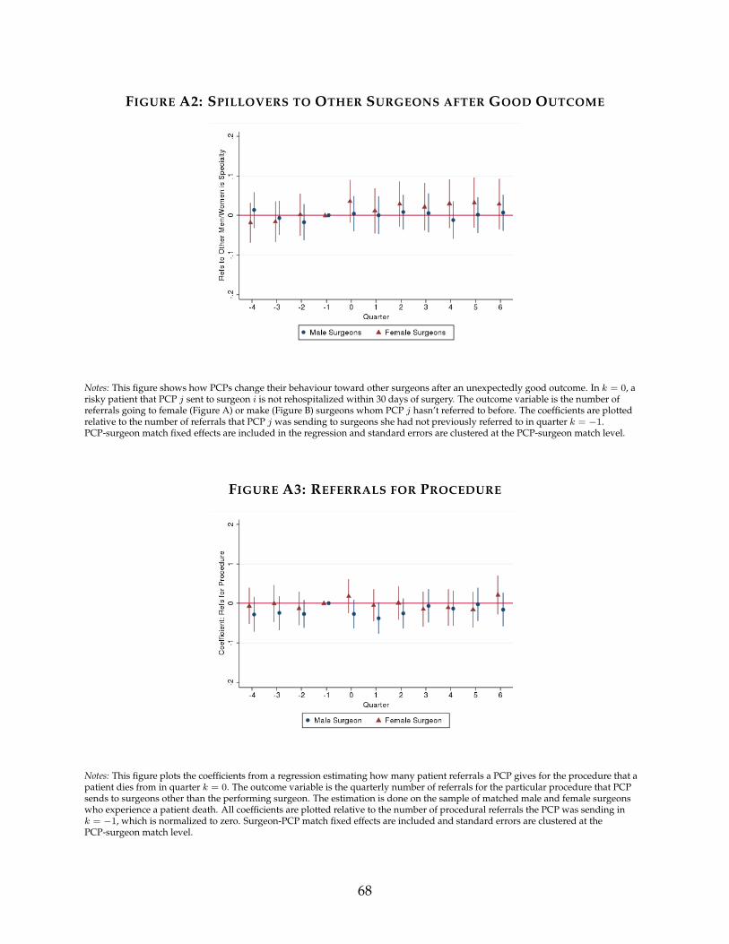
FIGURE A2: SPILLOVERS TO OTHER SURGEONS AFTER GOOD OUTCOME

Notes: This figure shows how PCPs change their behaviour toward other surgeons after an unexpectedly good outcome. In k = 0, arisky patient that PCP j sent to surgeon i is not rehospitalized within 30 days of surgery. The outcome variable is the number ofreferrals going to female (Figure A) or make (Figure B) surgeons whom PCP j hasn’t referred to before. The coefficients are plottedrelative to the number of referrals that PCP j was sending to surgeons she had not previously referred to in quarter k = −1.PCP-surgeon match fixed effects are included in the regression and standard errors are clustered at the PCP-surgeon match level.

FIGURE A3: REFERRALS FOR PROCEDURE

Notes: This figure plots the coefficients from a regression estimating how many patient referrals a PCP gives for the procedure that apatient dies from in quarter k = 0. The outcome variable is the quarterly number of referrals for the particular procedure that PCPsends to surgeons other than the performing surgeon. The estimation is done on the sample of matched male and female surgeonswho experience a patient death. All coefficients are plotted relative to the number of procedural referrals the PCP was sending ink = −1, which is normalized to zero. Surgeon-PCP match fixed effects are included and standard errors are clustered at thePCP-surgeon match level.

68

FIGURE A4: REFERRALS FOR OTHER PROCS. TO PERFORMING SURGEON

Notes: This figure shows the number of patients that PCP j refers to surgeon i for a procedure other that the patient who died wasreferred for. In k = 0, a patient that j referred to i for procedure n dies. The outcome variable is the number of referrals that j refers toi in each quarter for any procedure other than n. The coefficients are plotted relative to k = −1 and 95% confidence intervals are alsoshown. The coefficients for k = 1 through k = 6 are jointly significantly different from zero at the 10% level for both male and femalesurgeons. The sample used is the sample of matched surgeons who experienced a patient death. Surgeon-PCP match fixed effects areincluded. Standard errors are clustered at the PCP-surgeon match level.

69

FIGURE A5: DEATHS THAT OCCUR ON DAY OF SURGERY

Notes: This figure plots the quarterly regression coefficients and 95% confidence intervals from estimating equation 3 using thesample of matched male and female surgeons who experience a patient death that occurs within 24 hours of surgery. The coefficientsare plotted relative to the number of referrals the surgeon was receiving from the PCP in k = −1, which are normalized to zero. Ink = −1, male and female surgeons both received an average of 0.65 referrals from PCP j. A patient that PCP j referred to surgeon idies in k = 0. The outcome variable is the total number of referrals that PCP j sends to surgeon i each quarter. Standard errors areclustered at the PCP-surgeon match level.

FIGURE A6: UNEXPECTEDLY GOOD OUTCOMES: TOP 5% RISK LEVEL

Notes: This figure plots the quarterly coefficients and 95% confidence intervals from estimating equation 3, looking at good events.Here, good events are defined using a 5% risk cutoff rather than a 1% risk cutoff. All coefficients are plotted relative to the number ofreferrals the surgeon was receiving from the PCP in k = −1, which are normalized to zero. Standard errors are clustered at thePCP-surgeon match level.

70