interpreting random forest classiﬁcation models using a ... · interpreting random forest...

Interpreting random forest classification modelsusing a feature contribution method

Anna Palczewska∗1 and Jan Palczewski† 2 Richard Marchese Robinson‡3 DanielNeagu§1

1Department of Computing, University of Bradford, BD7 1DP Bradford, UK2School of Mathematics, University of Leeds, LS2 9JT Leeds, UK

3School of Pharmacy and Biomolecular Sciences, , Liverpool John MooresUniversity, L3 3AF Liverpool, UK

Abstract

Model interpretation is one of the key aspects of the model evaluationprocess. The explanation of the relationship between model variables andoutputs is relatively easy for statistical models, such as linear regressions,thanks to the availability of model parameters and their statistical signif-icance. For “black box” models, such as random forest, this informationis hidden inside the model structure. This work presents an approach forcomputing feature contributions for random forest classification models. Itallows for the determination of the influence of each variable on the modelprediction for an individual instance. By analysing feature contributions fora training dataset, the most significant variables can be determined and theirtypical contribution towards predictions made for individual classes, i.e.,class-specific feature contribution ”patterns”, are discovered. These patternsrepresent a standard behaviour of the model and allow for an additional as-sessment of the model reliability for a new data. Interpretation of featurecontributions for two UCI benchmark datasets shows the potential of theproposed methodology. The robustness of results is demonstrated throughan extensive analysis of feature contributions calculated for a large numberof generated random forest models.

∗[email protected]†[email protected]‡[email protected]§[email protected]

1

arX

iv:1

312.

1121

v1 [

cs.L

G]

4 D

ec 2

013

1 IntroductionModels are used to discover interesting patterns in data or to predict a specific out-come, such as drug toxicity, client shopping purchases, or car insurance premium.They are often used to support human decisions in various business strategies.This is why it is important to ensure model quality and to understand its out-comes. Good practice of model development [17] involves: 1) data analysis 2)feature selection, 3) model building and 4) model evaluation. Implementing thesesteps together with capturing information on how the data was harvested, howthe model was built and how the model was validated, allows us to trust that themodel gives reliable predictions. But, how to interpret an existing model? How toanalyse the relation between predicted values and the training dataset? Or whichfeatures contribute the most to classify a specific instance?

Answers to these questions are considered particularly valuable in such do-mains as chemoinformatics, bioinformatics or predictive toxicology [15]. Lin-ear models, which assign instance-independent coefficients to all features, are themost easily interpreted. However, in the recent literature, there has been consid-erable focus on interpreting predictions made by non-linear models do not renderthemselves to straightforward methods for the determination of variable/featureinfluence. In [8], the authors present a method for a local interpretation of Sup-port Vector Machine (SVM) and Random Forest models by retrieving the variablecorresponding to the largest component of the decision-function gradient at anypoint in the model. Interpretation of classification models using local gradientsis discussed in [4]. A method for visual interpretation of kernel-based predictionmodels is described in [11]. Another approach, which is presented in detail later,was proposed in [12] and aims at shedding light at decision-making process ofregression random forests.

Of interest to this paper is a popular “black-box” model – the random forestmodel [5]. Its author suggests two measures of the significance of a particularvariable [6]: the variable importance and the Gini importance. The variable im-portance is derived from the loss of accuracy of model predictions when valuesof one variable are permuted between instances. Gini importance is calculatedfrom the Gini impurity criterion used in the growing of trees in the random forest.However, in [16], the authors showed that the above measures are biased in favorof continuous variables and variables with many categories. They also demon-strated that the general representation of variable importance is often insufficientfor the complete understanding of the relationship between input variables and thepredicted value.

Following the above observation, Kuzmin et al. propose in [12] a new tech-nique to calculate a feature contribution, i.e., a contribution of a variable to theprediction, in a random forest model. Their method applies to models generated

2

for data with numerical observed values (the observed value is a real number). Un-like in the variable importance measures [6], feature contributions are computedseparately for each instance/record. They provide detailed information about re-lationships between variables and the predicted value. It is the extent and thekind of influence (positive/negative) of a given variable. This new approach waspositively tested in [12] on a Quantitative Structure-Activity (QSAR) model forchemical compounds. The results were not only informative about the structureof the model but also provided valuable information for the design of new com-pounds.

The procedure from [12] for the computation of feature contributions appliesto random forest models predicting numerical observed values. This paper aims toextend it to random forest models with categorical predictions, i.e., where the ob-served value determines one from a finite set of classes. The difficulty of achievingthis aim lies in the fact that a discrete set of classes does not have the algebraicstructure of real numbers which the approach presented in [12] relies on. Due tothe high-dimensionality of the calculated feature contributions, their direct analy-sis is not easy. We develop three techniques for discovering class-specific featurecontribution ”patterns” in the decision-making process of random forest models:the analysis of median feature contributions, of clusters and log-likelihoods. Thisfacilitates interpretation of model predictions as well as allows a more detailedanalysis of model reliability for an unseen data.

The paper is organised as follows. Section 2 provides a brief descriptionof random forest models. Section 3 presents our approach for calculating fea-ture contributions for binary classifiers, whilst Section 4 describes its extensionto multi-class classification problems. Section 5 introduces three techniques forfinding patterns in feature contributions and linking them to model predictions.Section 6 contains applications of the proposed methodology to two real worlddatasets from the UCI Machine Learning repository. Section 7 concludes the workpresented in this paper.

2 Random ForestA random forest (RF) model introduced by Breiman [5] is a collection of treepredictors. Each tree is grown according to the following procedure [6]:

1. the bootstrap phase: select randomly a subset of the training dataset – alocal training set for growing the tree. The remaining samples in the trainingdataset form a so-called out-of-bag (OOB) set and are used to estimate theRF’s goodness-of-fit.

2. the growing phase: grow the tree by splitting the local training set at each

3

node according to the value of one variable from a randomly selected subsetof variables (the best split) using classification and regression tree (CART)method [7].

3. each tree is grown to the largest extent possible. There is no pruning.

The bootstrap and growing phases require an input of random quantities. It isassumed that these quantities are independent between trees and identically dis-tributed. Consequently, each tree can be viewed as sampled independently fromthe ensemble of all tree predictors for a given training dataset.

For prediction, an instance is run through each tree in a forest down to a ter-minal node which assigns it a class. Predictions supplied by the trees undergo avoting process: the forest returns ca class with the maximum number of votes.Draws are resolved through a random selection.

To present our feature contribution procedure in the following section, we haveto develop a probabilistic interpretation of the forest prediction process. Denoteby C = {C1, C2, . . . , CK} the set of classes and by ∆K the set

∆K ={

(p1, . . . , pK) :K∑k=1

pk = 1 and pk ≥ 0}.

An element of ∆K can be interpreted as a probability distribution over C. Let ekbe an element of ∆K with 1 at position k – a probability distribution concentratedat class Ck. If a tree t predicts that an instance i belongs to a class Ck then wewrite Yi,t = ek. This provides a mapping from predictions of a tree to the set ∆K

of probability measures on C. Let

Yi =1

T

T∑t=1

Yi,t, (1)

where T is the overall number of trees in the forest. Then Yi ∈ ∆K and theprediction of the random forest for the instance i coincides with a class Ck forwhich the k-th coordinate of Yi is maximal.1

3 Feature Contributions for Binary ClassifiersThe set ∆K simplifies considerably when there are two classes, K = 2. Anelement p ∈ ∆K is uniquely represented by its first coordinate p1 (p2 = 1 −

1The distribution Yi is calculated by the function predict in the R package randomForest[13] when the type of prediction is set to prob.

4

p1). Consequently, the set of probability distributions on C is equivalent to theprobability weight assigned to class C1.

Before we present our method for computing feature contributions, we haveto examine the tree growing process. After selecting a training set, it is positionedin the root node. A splitting variable (feature) and a splitting value are selectedand the set of instances is split between the left and the right child of the rootnode. The procedure is repeated until all instances in a node are in the same classor further splitting does not improve prediction. The class that a tree assigns toa terminal node is determined through majority voting between instances in thatnode.

We will refer to instances of the local training set that pass through a givennode as the training instances in this node. The fraction of the training instancesin a node n belonging to class C1 will be denoted by Y n

mean. This is the probabilitythat a randomly selected element from the training instances in this node is in thefirst class. In particular, a terminal node is assigned to class C1 if Y n

mean > 0.5 orY nmean = 0.5 and the draw is resolved in favor of class C1.

The feature contribution procedure for a given instance involves two steps:1) the calculation of local increments of feature contributions for each tree and2) the aggregation of feature contributions over the forest. A local incrementcorresponding to a feature f between a parent node (p) and a child node (c) in atree is defined as follows:

LIcf =

Y cmean − Y p

mean,if the split in the parentis performed over thefeature f ,

0, otherwise.

A local increment for a feature f represents the change of the probability of beingin class C1 between the child node and its parent node provided that f is the split-ting feature in the parent node. It is easy to show that the sum of these changes,over all features, along the path followed by an instance from the root node to theterminal node in a tree is equal to the difference between Ymean in the terminaland the root node.

The contribution FCfi,t of a feature f in a tree t for an instance i is equal to

the sum of LIf over all nodes on the path of instance i from the root node to aterminal node. The contribution of a feature f for an instance i in the forest isthen given by

FCfi =

1

T

T∑t=1

FCfi,t. (2)

The feature contributions vector for an instance i consists of contributions FCfi

of all features f .

5

Notice that if the following condition is satisfied:

(U) for every tree in the forest, local training instances in each terminal node areof the same class

then Yi representing forest’s prediction (1) can be written as

Yi =(Y r +

∑f

FCfi , 1− Y r −

∑f

FCfi

)(3)

where Y r is the coordinate-wise average of Ymean over all root nodes in the forest.If this unanimity condition (U) holds, feature contributions can be used to retrievepredictions of the forest. Otherwise, they only allow for the interpretation of themodel.

3.1 ExampleWe will demonstrate the calculation of feature contributions on a toy exampleusing a subset of the UCI Iris Dataset [3]. From the original dataset, ten recordswere selected – five for each of two types of the iris plant: versicolor (class 0)and virginica (class 1) (see Table 1). A plant is represented by four attributes:Sepal.Length (f1), Sepal.Width (f2), Petal.Length (f3) and Petal.Width (f4). Thisdataset was used to generate a random forest model with two trees, see Figure 1.In each tree, the local training set (LD) in the root node collects those recordswhich were chosen by the random forest algorithm to build that tree. The LD setsin the child nodes correspond to the split of the above set according to the value ofa selected feature (it is written between branches). This process is repeated untilreaching terminal nodes of the tree. Notice that the condition (U) is satisfied – forboth trees, each terminal node contains local training instances of the same class:Ymean is either 0 or 1.

The process of calculating feature contributions runs in 2 steps: the determi-nation of local increments for each node in the forest (a preprocessing step) andthe calculation of feature contributions for a particular instance. Figure 1 showsY nmean and the local increment LIcf for a splitting feature f in each node. Having

computed these values, we can calculate feature contributions for an instance byrunning it through both trees and summing local increments of each of the fourfeatures. For example, the contribution of a given feature for the instance x1 is cal-culated by summing local increments for that feature along the path p1 = n0 → n1

in tree T1 and the path p2 = n0 → n1 → n4 → n5 in tree T2. According to For-mula (2) the contribution of feature f2 is calculated as

FCf2x1

=1

2

(0 +

1

4

)= 0.125

6

Table 1: Selected records from the UCI Iris Dataset. Each record corresponds to aplant. The plants were classified as iris versicolor (class 0) and virginica (class 1).

Sepal PetalLength (f1) Width (f2) Length (f3) Width (f4) class

x1 6.4 3.2 4.5 1.5 0x2 6.3 2.5 4.9 1.5 0x3 6.4 2.9 4.3 1.3 0x4 5.5 2.5 4.0 1.3 0x5 5.5 2.6 4.4 1.2 0x6 7.7 3.0 6.1 2.3 1x7 6.4 3.1 5.5 1.8 1x8 6.0 3.0 4.8 1.8 1x9 6.7 3.3 5.7 2.5 1x10 6.5 3.0 5.2 2.0 1

and the contribution of feature f3 is

FCf3x1

=1

2

(− 3

7− 9

28− 1

2

)= −0.625.

The contributions of features f1 and f4 are equal to 0 because these attributes arenot used in any decision made by the forest. The predicted probability Yx1 that x1belongs to class 1 (see Formula (3)) is

Yx1 =1

2

(3

7+

4

7

)︸︷︷︸

Y r

+(0 + 0.125− 0.625 + 0

)︸︷︷︸∑f FCf

x1

= 0.0

Table 2 collects feature contributions for all 10 records in the example dataset.These results can be interpreted as follows:

• for instances x1, x3, the contribution of f2 is positive, i.e., the value of thisfeature increases the probability of being in class 1 by 0.125. However, thelarge negative contribution of the feature f3 implies that the value of thisfeature for instances x1 and x3 was decisive in assigning the class 0 by theforest.

• for instances x6, x7, x9, the decision is based only on the feature f3.

• for instances x2, x4, x5, the contribution of both features leads the forestdecision towards class 0.

7

6

Figure 1: A random forest model for the dataset from Table 1. The set LD in theroot node contains a local training set for the tree. The sets LD in the child nodescorrespond to the split of the above set according to the value of selected feature.In each node, Y n

mean denotes the fraction of instances in the LD set in this nodebelonging to class 1, whilst LInf shows non-zero local increments.

• for instances x8, x10, Y is 0.5. This corresponds to the case where one ofthe trees points to class 0 and the other to class 1. In practical applications,such situations are resolved through a random selection of the class. SinceY r = 0.5, the lack of decision of the forest has a clear interpretation interms of feature contributions: the amount of evidence in favour of oneclass is counterbalanced by the evidence pointing towards the other.

4 Feature Contributions for General ClassifiersWhen K > 2, the set ∆K cannot be described by a one-dimensional value asabove. We, therefore, generalize the quantities introduced in the previous sectionto a multi-dimensional case. Y n

mean in a node n is an element of ∆K , whose k-thcoordinate, k = 1, 2, . . . , K, is defined as

Y nmean,k =

|{i ∈ TS(n) : i ∈ Ck}||TS(n)|

, (4)

8

Table 2: Feature contributions for the random forest model from Figure 1.

Sepal PetalY Length (f1) Width (f2) Length (f3) Width (f4) prediction

x1 0.0 0 0.125 -0.625 0 0x2 0.0 0 -0.125 -0.375 0 0x3 0.0 0 0.125 -0.625 0 0x4 0.0 0 -0.125 -0.375 0 0x5 0.0 0 -0.125 -0.375 0 0x6 1.0 0 0 0.5 0 1x7 1.0 0 0 0.5 0 1x8 0.5 0 0.125 -0.125 0 ?x9 1.0 0 0 0.5 0 1x10 0.5 0 0 0 0 ?

where TS(n) is the set of training instances in the node n and | · | denotes thenumber of elements of a set. Hence, if an instance is selected randomly from a lo-cal training set in a node n, the probability that this instance is in class Ck is givenby the k-th coordinate of the vector Y n

mean. Local increment LIcf is analogouslygeneralized to a multidimensional case:

LIcf =

Y cmean − Y p

mean,if the split in the parentis performed over thefeature f ,

(0, . . . , 0)︸︷︷︸K times

, otherwise,

where the difference is computed coordinate-wise. Similarly, FCfi,t and FCf

i areextended to vector-valued quantities. Notice that if the condition (U) is satisfied,Equation (3) holds with Y r being a coordinate-wise average of vectors Y n

mean overall root nodes n in the forest.

Take an instance i and let Ck be the class to which the forest assigns thisinstance. Our aim is to understand which variables/features drove the forest tomake that prediction. We argue that the crucial information is the one whichexplains the value of the k-th coordinate of Yi. Hence, we want to study the k-thcoordinate of FCf

i for all features f .Pseudo-code to calculate feature contributions for a particular instance to-

wards the class predicted by the random forest is presented in Algorithm 1. Itsinputs consist of a random forest model RF and an instance i which is repre-sented as a vector of feature values. In line 1, k ∈ {1, 2, . . . , K} is assigned theindex of a class predicted by the random forest RF for the instance i. The follow-ing line creates a vector of real numbers indexed by features and initialized to 0.

9

Then for each tree in the forest RF the instance i is run down the tree and featurecontributions are calculated. The quantity SplitFeature(parent) identifies a fea-ture f on which the split is performed in the node parent. If the value i(f) of thatfeature f for the instance i is lower or equal to the threshold SplitV alue(parent),the route continues to the left child of the node parent. Otherwise, it goes to theright child (each node in the tree has either two children or is a terminal node).A position corresponding to the feature f in the vector FC is updated accordingto the change of value of Ymean,k, i.e., the k-th coordinate of Ymean, between theparent and the child.

Algorithm 1 FC(RF ,i)

1: k ← forest predict(RF, i)2: FC ← vector(features)3: for each tree T in forest F do4: parent← root(T )5: while parent ! = TERMINAL do6: f ← SplitFeature(parent)7: if i[f ] <= SplitV alue(parent) then8: child← leftChild(parent)9: else

10: child← rightChild(parent)11: end if12: FC[f ]← FC[f ] + Y child

mean,k − Yparentmean,k

13: parent← child14: end while15: end for16: FC ← FC / nTrees(F )17: return FC

Algorithm 2 provides a sketch of the preprocessing step to compute Y nmean for

all nodes n in the forest. The parameter D denotes the set of instances used fortraining of the forest RF . In line 2, TS is assigned the set used for growing treeT . This set is further split in nodes according to values of splitting variables. Wepropose to use DFS (depth first search [9]) to traverse the tree and compute thevector Y n

mean once a training set for a node n is determined. There is no need tostore a training set for a node n once Y n

mean has been calculated.

10

Algorithm 2 Ymean(RF,D)

1: for each tree T in forest F do2: TS ← training set for tree T3: use DFS algorithm to compute training sets in all other nodes n of tree T

and compute the vector Y nmean according to formula (4).

4: end for

5 Analysis of Feature ContributionsFeature contributions provide the means to understand mechanisms that lead themodel towards particular predictions. This is important in chemical or biologi-cal applications where the additional knowledge of the forest’s decision-makingprocess can inform the development of new chemical compounds or explain theirinteractions with living organisms. Feature contributions may also be useful forassessing the reliability of model predictions for unseen instances. They providecomplementary information to forest’s voting results. This section proposes threetechniques for finding patterns in the way a random forest uses available featuresand linking these patterns with the forest’s predictions.

5.1 MedianThe median of a sequence of numbers is such a value that the number of elementsbigger than it and the number of elements smaller than it is identical. When thenumber of elements in the sequence is odd, this is the central elements of thesequence. Otherwise, it is common to take the midpoint between the two mostcentral elements. In statistics, the median is an estimator of the expectation whichis less affected by outliers than the sample mean. We will use this property ofthe median to find a “standard level” of feature contributions for representativesof a particular class. This standard level will facilitate an understanding of whichfeatures are instrumental for the classification. It can also be used to judge thereliability of forest’s prediction for an unseen instance.

For a given random forest model, we select those instances from the trainingdataset that are classified correctly. We calculate the medians of contributionsof every feature separately for each class. The medians computed for one classare combined into a vector which is interpreted as providing the aforementioned“standard level” for this class. If most of instances from the training dataset be-longing to a particular class are close to the corresponding vector of medians, wemay treat this vector justifiably as a standard level. When a prediction is requestedfor a new instance, we query the random forest model for the fraction of trees vot-ing for each class and calculate feature contributions leading to its final prediction.

11

If a high fraction of trees votes for a given class and the feature contributions areclose to the standard level for this class, we may reasonably rely on the prediction.Otherwise we may doubt the random forest model prediction.

It may, however, happen that many instances from the training dataset cor-rectly predicted to belong to a particular class are distant from the correspondingvector of medians. This might suggest that there is more than one standard level,i.e., there are multiple mechanisms relating features to correct classes. The nextsubsection presents more advanced methods capable of finding a number of stan-dard levels – distinct patterns followed by the random forest model in its predic-tion process.

5.2 Cluster AnalysisClustering is an approach for grouping elements/objects according to their similar-ity [10]. This allows us to discover patterns that are characteristic for a particulargroup. As we discussed above, feature contributions in one class may have morethan one ”standard level”. When this is discovered, clustering techniques can beemployed to find if there is a small number of distinct standard levels, i.e., featurecontributions of the instances in the training dataset group around a few pointswith only a relatively few instances being far away from them. These few in-stances are then treated as unusual representatives of a given class. We shall referto clusters of instances around these standard levels as ”core clusters”.

The analysis of core clusters can be of particular importance for applications.For example, in the classification of chemical compounds, the split into clustersmay point to groups of compounds with different mechanisms of activity. Weshould note that the similarity of feature contributions does not imply that partic-ular features are similar. We examined several examples and noticed that cluster-ing based upon the feature values did not yield useful results whereas the samemethod applied to feature contributions was able to determine a small number ofcore clusters.

Figure 2 demonstrates the process of analysis of model reliability for a newinstance using cluster analysis. In a preprocessing phase, feature contributionsfor instances in the training dataset are obtained. The optimal number of clustersfor each class can be estimated by using, e.g., the Akaike information criterion(AIC), the Bayesian information criterion (BIC) or the Elbow method [10, 14].We noticed that these methods should not be rigidly adhered to: their underlyingassumption is that the data is clustered and we only have to determine the numberof these clusters. As we argued above, we expect feature contributions for variousinstances to be grouped into a small number of clusters and we accept a reasonablenumber outliers interpreted as unusual instances for a given class. Clusteringalgorithms try to push those outliers into clusters, hence increasing their number

12

RF Model

Training DataFeature Contributions

f11

, f12

, …, f1n

. .

. . .fm1

, fm2

, ..., fmn

Cluster Analysis

New instance

Predictions

f1, f

2, ...,

fn

Decision

PREPROCESSING

Figure 2: The workflow for assessing the reliability of the prediction made by arandom forest (RF) model.

unnecessarily. We recommend, therefore, to treat the calculated optimal numberof clusters as the maximum value and consecutively decrease it looking at thestructure and performance of the resulting clusters: for each cluster we assessthe average fraction of trees voting for the predicted class across the instancesbelonging to this cluster as well as the average distance from the centre of thecluster. Relatively large clusters with the former value close to 1 and the lattervalue small form the group of core clusters.

To assess the reliability of the model prediction for a new instance, we rec-ommend looking at two measures: the fraction of trees voting for the predictedclass as well as the cluster to which the instance is assigned based on its featurecontributions. If the cluster is one of the core clusters and the distance from itscentre is relatively small, the instance is a typical representative of its predictedclass. This together with high decisiveness of the forest suggests that the model’sprediction should be trusted. Otherwise, we should allow for an increased chanceof misclassification.

5.3 Log-likelihoodFeature contributions for a given instance form a vector in a multi-dimensionalEuclidean space. Using a popular k-mean clustering method, for each class we

13

divide vectors corresponding to feature contributions of instances in the trainingdataset into groups minimizing the Euclidean distance from the centre in eachgroup. Figure 3 shows a box-plot of feature contributions for instances in a corecluster in a hypothetical random forest model. Notice that some features are sta-ble within a cluster – the height of the box is small. Others (F1 and F4) displayhigher variability. One would therefore expect that the same divergence of contri-butions for features F3 and F4 from their mean value should be treated differently.It is more significant for the feature F3 than for the feature F4. This is unfortu-nately not taken into account when the Euclidean distance is considered. Here, wepropose an alternative method for assessing the distance from the cluster centrewhich takes into account the variation of feature contributions within a cluster.Our method has probabilistic roots and we shall present it first from a statisticalpoint of view and provide other interpretations afterwards.

F1 F2 F3 F4

−0.1

00.0

00.1

00.2

0

Feature

Featu

re c

ontr

ibution

Figure 3: The box-plot for feature contributions within a core cluster for a hypo-thetical random forest model.

We assume that feature contributions for instances within a cluster share thesame base values (µf ) - the centre of the cluster. We attribute all discrepanciesbetween this base value and the actual feature contributions to a random pertur-bation. These perturbations are assumed to be normally distributed with the mean0 and the variance σ2

f , where f denotes the feature. The variance of the perturba-tion for each feature is selected separately – we use the sample variance computedfrom feature contributions of instances of the training dataset belonging to thiscluster. Although it is clear that perturbations for different features exhibit somedependence, it is impossible to assess it given the number of instances in a cluster

14

and a large number of features typically in use.2 Therefore, we resort to a commonsolution: we assume that the dependence between perturbations is small enoughto justify treating them as independent. Summarising, our statistical model for thedistribution of feature contributions within a cluster is as follows: feature contri-butions for instances within a cluster are composed of a base value and a randomperturbation which is normally distributed and independent between features.

Take an instance iwith feature contributions FCfi . The log-likelihood of being

in a cluster with the centre (µf ) and variances of perturbations (σ2f ) is given by

LLi =∑f

(− (FCf

i − µf )2

2σ2f

− 1

2log(2πσ2

f )). (5)

The higher the log-likelihood the bigger the chance of feature contributions of theinstance i to belong to the cluster. Notice that the above sum takes into account theobservations we made at the beginning of this subsection. Indeed, as the secondterm in the sum above is independent of the considered instance, the log-likelihoodis equivalent to ∑

f

(− (FCf

i − µf )2

2σ2f

),

which is the negative of the squared weighted Euclidean distance between FCfi

and µf . The weights being inversely proportional to the variability of a givenfeature contribution in the training instances in the cluster. In our toy exampleof Figure 3, this corresponds to penalizing more for discrepancies for features F2and F3, and significantly less for discrepancies for features F1 and F4.

In the following section, we analyse relations between the log-likelihood andclassification for a UCI Breast Cancer Wisconsin Dataset.

6 ApplicationsIn this section, we demonstrate how the techniques from the previous section canbe applied to improve understanding of a random forest model. We consider oneexample of a binary classifier using the UCI Breast Cancer Wisconsin Dataset [1](BCW Dataset) and one example of a general classifier for the UCI Iris Dataset[3]. We complement our studies with a robustness analysis.

2A covariance matrix of feature contribution has F (F + 1)/2 distinct entries, where F is thenumber of features. This value is usually larger than the size of a cluster making it impossible toretrieve useful information about the dependence structure of feature contributions. Applicationof more advanced methods, such as principal component analysis, is left for future research.

15

6.1 Breast Cancer Wisconsin DatasetThe UCI Breast Cancer Wisconsin Dataset contains characteristics of cell nucleifor 569 breast tissue samples; 357 are diagnosed as benign and 212 as malignant.The characteristics were captured from a digitized image of a fine needle aspi-rate (FNA) of a breast mass. There are 30 features, three (the mean, the standarderror and the average of the three largest values) for each of the following 10 char-acteristics: radius, texture, perimeter, area, smoothness, compactness, concavity,concave points, symmetry and fractal dimension. For brevity, we numbered thesefeatures from F1 to F30 according to their order in the data file.

To reduce correlation between features and facilitate model interpretation, themin-max (minimal-redundancy-maximal-relevance) method was applied and thefollowing features were removed from the dataset: 1, 3, 8, 10, 11, 12, 13, 15, 19,20, 21, 24, 26. A random forest model was generated on 2/3 randomly selectedinstances using 500 trees. The other 1/3 of instances formed the testing dataset.The validation showed that the model accuracy was 0.9682 (only 6 instances outof 189 were classified incorrectly); similar accuracy was achieved when the modelwas generated using all the features.

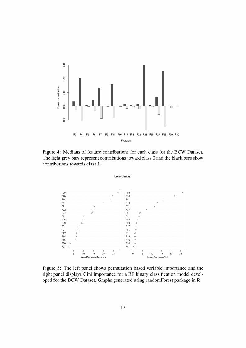
We applied our feature contribution algorithm to the above random forest bi-nary classifier. To align notation with the rest of the paper, we denote the class“malignant” by 1 and the class “benign” by 0. Aggregate results for the featurecontributions for all training instances and both classes are presented in Figure 4.Light-grey bars show medians of contributions for instances of class 0, whereasblack bars show medians of contributions for instances of class 1 (malignant). No-tice that there are only a few significant features in the graph: F4 – the mean ofthe cell area, F7 – the mean of the cell concavity, F14 – the standard deviation ofthe cell area, F23 – the average of three largest measurements of the cell perime-ter and F28 – the average of three largest measurements of concave points. Thisselection of significant features is perfectly in agreement with the results of thepermutation based variable importance (the left panel of Figure 5) and the Giniimportance (the right panel of Figure 5). Interpreting the size of bars as the levelof importance of a feature, our results are in line with those provided by the Giniindex. However, the main advantage of the approach presented in this paper liesin the fact that one can study the reasons for the forest’s decision for a particularinstance.

Comparison of feature contributions for a particular instance with medians offeature contributions for all instances of one class provides valuable informationabout the forest’s prediction. Take an instance predicted to be in class 1. In atypical case when the large majority of trees votes for class 1 the feature contri-butions for that instance are very close to the median values (see Figure 6a). Thishappens for around 80% of all instances from the testing dataset predicted to be

16

F2 F4 F5 F6 F7 F9 F14 F16 F17 F18 F22 F23 F25 F27 F28 F29 F30

Features

Featu

re c

ontr

ibution

−0.0

50

.00

0.0

50.1

00.1

5

Figure 4: Medians of feature contributions for each class for the BCW Dataset.The light grey bars represent contributions toward class 0 and the black bars showcontributions towards class 1.

F9

F30

F16

F18

F17

F6

F5

F29

F25

F2

F27

F22

F7

F4

F14

F28

F23

5 10 15 20 25

MeanDecreaseAccuracy

F9

F30

F16

F18

F5

F25

F17

F29

F22

F2

F6

F27

F7

F14

F4

F28

F23

0 5 10 15 20 25

MeanDecreaseGini

breastrfmtest

Figure 5: The left panel shows permutation based variable importance and theright panel displays Gini importance for a RF binary classification model devel-oped for the BCW Dataset. Graphs generated using randomForest package in R.

17


Features

Fe

atu

re c

ontr

ibution

0.0

00.0

20.0

40.0

60.0

80

.10

0.1

20.1

4

(a)


Features

Fea

ture

co

ntr

ibu

tio

n

−0.1

0−

0.0

50.0

00

.05

0.1

00

.15

(b)

Figure 6: Comparison of the medians of feature contributions (toward class 1)over all instances of class 1 (black bars) with a) feature contributions for instancenumber 3 (light-grey bars) b) feature contributions for instances number 194 (greybars) and 537 (light-grey bars) from the BCW Dataset. The fractions of treesvoting for class 0 and 1 for these three instances are collected in Table 3.

18

Table 3: Percentage of trees that vote for each class in RF model for a selection ofinstances from the BCW Dataset.

Instance Id benign (class 0) malignant (class 1)3 0 1

194 0.298 0.702537 0.234 0.766

in class 1. However, when the decision is less unanimous, the analysis of featurecontributions may reveal interesting information. As an example, we have choseninstances 194 and 537 (see Table 3) which were classified correctly as malignant(class 1) by a majority of trees but with a significant number of trees expressingan opposite view. Figure 6b presents feature contributions for these two instances(grey and light grey bars) against the median values for class 1 (black bars). Thelargest difference can be seen for the contributions of very significant featuresF23, F4 and F14: it is highly negative for the two instances under considerationcompared to a large positive value commonly found in instances of class 1. Re-call that a negative value contributes towards the classification in class 0. Thereare also three new significant attributes (F2, F22 and F27) that contribute towardsthe correct classification as well as unusual contributions for features F7 and F28.These newly significant features are judged as only moderately important by bothof the variable importance methods in Figure 5. It is, therefore, surprising to notethat the contribution of these three new features was instrumental in correctly clas-sifying instances 194 and 537 as malignant. This highlights the fact that featureswhich may not generally be important for the model may, nonetheless, be im-portant for classifying specific instances. The approach presented in this paper isable to identify such features, whilst the standard variable importance measuresfor random forest cannot.

6.2 Cluster Analysis and Log-likelihoodThe training dataset previously derived for the BCW Dataset was partitioned ac-cording to the true class labels. A clustering algorithm implemented in the Rpackage kmeans was run separately for each class. This resulted in the determi-nation of three clusters for class 0 and three clusters for class 1. The structureand size of clusters is presented in Table 4. Each class has one large cluster: clus-ter 3 for class 0 and cluster 2 for class 1. Both have a bigger concentration ofpoints around the cluster centre (small average distance) than the remaining clus-ters. This suggests that there is exactly one core cluster corresponding to a class.This explains the success of the analysis based on the median as the vectors of

19

medians are close to the centres of unique core clusters.

Table 4: The structure of clusters for BCW Dataset. For each cluster, the size(the number of training instances) is reported in the left column and the averageEuclidean distance from the cluster centre among the training dataset instancesbelonging to this cluster is displayed in the right column.

Cluster 1 Cluster 2 Cluster 3size avg. distance size avg. distance size avg. distance

class 0 12 0.220 16 0.262 213 0.068class 1 20 0.241 109 0.111 10 0.336

Figure 7 lends support to our interpretation of core clusters. The left panelshows the box-plot of the fraction of trees voting for class 0 among training in-stances belonging to each of the three clusters. A value close to one representspredictions for which the forest is nearly unanimous. This is the case for cluster3. Two other clusters comprise around 10% of the training instances for whichthe random forest model happened to be less decisive. A similar pattern can beobserved in the case of class 1, see the right panel of the same figure. The unanim-ity of the forest is observed for the most numerous cluster 2 with other clustersshowing lower decisiveness. The reason for this becomes clear once one looks atthe variability of feature contributions within each cluster, see Figure 8. The up-per and lower ends of the box corresponds to 25% and 75% quantiles, whereas thewhiskers show the full range of the data. Cluster 2 enjoys a minor variability of allthe contributions which supports our earlier claims of the similarity of instances(in terms of their feature contributions) in the core class. One can see much highervariability in two remaining clusters showing that the forest used different featuresas evidence to classify instances in each of these clusters. Although in cluster 2all contributions were positive, in clusters 1 and 3 there are features with nega-tive contributions. Recall that a negative value of a feature contribution providesevidence against being in the corresponding class, here class 1.

Based on the observation that clusters correspond to a particular decision-making route for the random forest model, we introduced the log-likelihood asa way to assess the distance of a given instance from the cluster centre, or, in aprobabilistic interpretation, to compute the likelihood3 that the instance belongsto the given cluster. It should however be clarified that one cannot compare thelikelihood for the core cluster in class 0 with the likelihood for the core cluster inclass 1. The likelihood can only be used for comparisons within one cluster: hav-ing two instances we can say which one is more likely to belong to a given cluster.By comparing it to a typical likelihood for training instances in a given cluster we

3The likelihood is obtained by applying the exponential function to the log-likelihood.

20

1 2 3

0.7

50.8

00.8

50.9

00.9

51.0

0

Cluster

Pro

babili

ty o

f cla

ss 0

(a) Class 0

1 2 3

0.7

0.8

0.9

1.0

Cluster

Pro

babili

ty o

f cla

ss 1

(b) Class 1

Figure 7: Fraction of forest trees voting for the correct class in each cluster fortraining part of the BCW Dataset.

21


−0.

2−

0.1

0.0

0.1

0.2

0.3

Feature

Fea

ture

con

trib

utio

n

(a) Cluster 1


−0.

2−

0.1

0.0

0.1

0.2

0.3

Feature

Fea

ture

con

trib

utio

n

(b) Cluster 2


−0.

2−

0.1

0.0

0.1

0.2

0.3

Feature

Fea

ture

con

trib

utio

n

(c) Cluster 3

Figure 8: Boxplot of feature contributions (towards class 1) for training instancesin each of three clusters obtained for class 1.

22

can further draw conclusions about how well an instance fits that cluster. Figure9 presents the log-likelihoods for the two core clusters (one for each class) forinstances from the testing dataset. Shapes are used to mark instances belongingto each class: circles for class 0 and triangles for class 1. Notice that likelihoodsprovide a very good split between classes: instances belonging to class 0 have ahigh log-likelihood for the core cluster of class 0 and rather low log-likelihood forthe core cluster of class 1. And vice-versa for instances of class 1.

−250 −200 −150 −100 −50 0 50 100

−500

−400

−300

−200

−100

0100

Log−likelihood for the core cluster in class 1

Log−

likelih

ood for

the c

ore

clu

ste

r in

cla

ss 0

Figure 9: Log-likelihoods for belonging to the core cluster in class 0 (vertical axis)and class 1 (horizontal axis) for the testing dataset in BCW. Circles correspond toinstances of class 0 while triangles denote instances of class 1.

6.3 Iris DatasetIn this section we use the UCI Iris Dataset [3] to demonstrate interpretability offeature contributions for multi-classification models. We generated a random for-est model on 100 randomly selected instances. The remaining 50 instances wereused to assess the accuracy of the model: 47 out of 50 instances were correctlyclassified. Then we applied our approach for determining the feature contributionsfor the generated model. Figure 10 presents medians of feature contributions foreach of the three classes. In contrast to the binary classification case, the medi-ans are positive for all classes. A positive feature contribution for a given class

23

means that the value of this feature directs the forest towards assigning this class.A negative value points towards the other classes.

Sepal.Length Sepal.Width Petal.Length Petal.Width

Setosa VersicolourVirginica

Feature

Fea

ture

con

trib

utio

n

0.00

0.05

0.10

0.15

0.20

0.25

0.30

0.35

Figure 10: Medians of feature contributions for each class for the UCI Iris Dataset.

Feature contributions provide valuable information about the reliability of ran-dom forest predictions for a particular instance. It is commonly assumed that themore trees voting for a particular class, the higher the chance that the forest deci-sion is correct. We argue that the analysis of feature contributions offers a morerefined picture. As an example, take two instances: 120 and 150. The first one wasclassified in class Versicolour (88% of trees voted for this class). The second onewas assigned class Virginica with 86% of trees voting for this class. We are, there-fore, tempted to trust both of these predictions to the same extent. Table 5 collectsfeature contributions for these instances towards their predicted classes. Recallthat the highest contribution to the decision is commonly attributed to features 3(Petal.Length) and 4 (Petal Width), see Figure 10. These features also make thehighest contributions to the predicted class for instance 150. The indecisivenessof the forest may stem from an unusual value for the feature 1 (Sepal.Length)which points towards a different class. In contrast, the instance 120 shows stan-

Table 5: Feature contributions towards predicted classes for selected instancesfrom the UCI Iris Dataset.

InstanceSepal Petal

Length Width Length Width120 0.059 0.014 0.053 0.448150 -0.097 0.035 0.259 0.339

24

−300 −250 −200 −150 −100 −50 0 50

−30

0−

250

−20

0−

150

−10

0 −

50

0 5

0

−2000000

−1500000

−1000000

−500000

0

500000

LH2LH

1

LH3

●●●●●●●●●●●

●●●●●

Figure 11: Log-likelihoods for all instances in UCI Iris Dataset towards core clus-ters for each class. Circles represent the Setosa class, triangles represent Versi-colour and diamonds represent the Virginica class. Points corresponding to thesame class tend to group together and there are only a few instances that are farfrom their cores.

dard (low) contributions of the first two features and unusual contributions of thelast two features: very low for feature 3 and high for feature 4. Recall that fea-tures 3 and 4 tend to contribute most to the forest’s decision (see Figure 10) withvalues between 0.25 and 0.35. The low value for feature 3 is non-standard for itspredicted class, which increases the chance of it being wrongly classified. Indeed,both instances belong to class Virginica while the forest classified the instance 120wrongly as class Versicolour and the instance 150 correctly as class Virginica.

The cluster analysis of feature contributions for the UCI Iris Dataset revealedthat it is sufficient to consider only two clusters for each class. Cluster sizes are 5

25

and 45 for class Setosa, 4 and 46 for class Versicolour and 5 and 44 for class Vir-ginica. Core clusters were straightforward to determine: for each class, the largestof the two clusters was selected as the core cluster. Figure 11 displays an analysisof log-likelihoods for all instances in the dataset. For every instance, we computedfeature contributions towards each class and calculated log-likelihoods of being inthe core clusters of the respective classes. On the graph, each point represents oneinstance. The coordinate LH1 is the log-likelihood for the core cluster of classSetosa, the coordinate LH2 is the log-likelihood for the core cluster of class Ver-sicolour and the coordinate LH3 is the log-likelihood for the core cluster of classVirginica. Shapes of points show the true classification: class Setosa is repre-sented by circles, Versicolour by triangles and Virginica by diamonds. Notice thatpoints corresponding to instances of the same class tend to group together. Thiscan be interpreted as the existence of coherent patterns in the reasoning of therandom forest model.

6.4 Robustness AnalysisFor the validity of the study of feature contributions, it is crucial that the results arenot artefacts of one particular realization of a random forest model but that theyconvey actual information held by the data. We therefore propose a method forrobustness analysis of feature contributions. We will use the UCI Breast CancerWisconsin Dataset studied in Subsection 6.1 as an example.

We removed instance number 3 from the original dataset to allow us to performtests with an unseen instance. We generated 100 random forest models with 500trees with each model built using an independent randomly generated training setwith 379 ≈ 2/3·568 instances. The rest of the dataset for each model was used forits validation. The average model accuracy was 0.963. For each generated model,we collected medians of feature contributions separately for training and testingdatasets and each class. The variation of these quantities over models for class 1and the training dataset are presented using a box plot in Figure 12a. The top ofthe box is the 75% quantile, the bottom is the 25% quantile, while the bold line inthe middle is the median (recalling that this is the median of the median featurecontributions across multiple models). Whiskers show the extent of minimal andmaximal values for each feature contribution. Notice that the variation betweensimulations is moderate and conclusions drawn for one realization of the randomforest model in Subsection 6.1 would hold for each of the generated 100 randomforest models.

A testing dataset contains those instances that do not take part in the modelgeneration. One can, therefore, expect more errors in the classification of theforest, which, in effect, should imply lower stability of the calculated feature con-tributions. Indeed, the box plot presented in Figure 12b shows a slight tendency

26


0.00

0.05

0.10

0.15

Feature

Fea

ture

con

trib

utio

n

(a) (a) Medians of feature contributions for training datasets


0.00

0.05

0.10

0.15

Feature

Fea

ture

con

trib

utio

n

(b) (b) Medians of feature contributions for testing datasets


0.00

0.05

0.10

0.15

Feature

Fea

ture

con

trib

utio

n

(c) (c) Feature contributions for an unseen instance

Figure 12: Feature contributions towards class 1 for 100 random forest models forthe BCW dataset.

27

towards increased variability of the feature contributions when compared to Fig-ure 12a. However, these results are qualitatively on a par with those obtained onthe training datasets. We can, therefore, conclude that feature contributions com-puted for a new (unseen) instance provide reliable information. We further testedthis hypothesis by computing feature contributions for instance number 3 that didnot take part in the generation of models. The statistics for feature contributionsfor this instance over 100 random forest models are shown in Figure 12c. Similarresults were obtained for other instances.

7 ConclusionsFeature contributions provide a novel approach towards black-box model interpre-tation. They measure the influence of variables/features on the prediction outcomeand provide explanations as to why a model makes a particular decision. In thiswork, we extended the feature contribution method of [12] to random forest clas-sification models and we proposed three techniques (median, cluster analysis andlog-likelihood) for finding patterns in the random forest’s use of available fea-tures. Using UCI benchmark datasets we showed the robustness of the proposedmethodology. We also demonstrated how feature contributions can be applied tounderstand the dependence between instance characteristics and their predictedclassification and to assess the reliability of the prediction. The relation betweenfeature contributions and standard variable importance measures was also inves-tigated. The software used in the empirical analysis was implemented in R asan add-on for the randomForest package and is currently being prepared forsubmission to CRAN [2] under the name rfFC.

Acknowledgements. This work is partially supported by BBSRC and Syn-genta Ltd through the Industrial CASE Studentship Grant (No. BB/H530854/1).

References[1] Breast Cancer Wisconsin Diagnostic dataset. http://archive.

ics.uci.edu/ml/datasets/Breast+Cancer+Wisconsin+\%28Diagnostic\%29.

[2] CRAN - The Comprehensive R Archive Network. http://cran.r-project.org/.

[3] Iris dataset. http://archive.ics.uci.edu/ml/datasets/Iris.

28

[4] David Baehrens, Timon Schroeter, Stefan Harmeling, Motoaki Kawanabe,Katja Hansen, and Klaus-Robert Muller. How to explain individual classi-fication decisions. Journal of Machine Learning Research, 11:1803–1831,2010.

[5] Leo Breiman. Random forests. Machine Learning, 45(1):5–32, 2001.

[6] Leo Breiman and Adele Cutler. Random forests. http://www.stat.berkeley.edu/˜breiman/RandomForests/, 2008.

[7] Leo Breiman, J. H. Friedman, R. A. Olshen, and C. J. Stone. Classificationand regression trees. Monterey, CA: Wadsworth & Brooks/Cole AdvancedBooks & Software, 1984.

[8] Lars Carlsson, Ernst Ahlberg Helgee, and Scott Boyer. Interpretation of non-linear qsar models applied to ames mutagenicity data. Journal of ChemicalInformation and Modeling, 49(11):2551–2558, 2009.

[9] Thomas H. Cormen, Clifford Stein, Ronald L. Rivest, and Charles E. Leis-erson. Introduction to Algorithms. McGraw-Hill Higher Education, 2ndedition, 2001.

[10] David J. Hand, Padhraic Smyth, and Heikki Mannila. Principles of datamining. MIT Press, Cambridge, MA, USA, 2001.

[11] Katja Hansen, David Baehrens, Timon Schroeter, Matthias Rupp, and Klaus-Robert Muller. Visual interpretation of kernel-based prediction models.Molecular Informatics, 30(9):817–826, 2011.

[12] Victor E. Kuz’min, Pavel G. Polishchuk, Anatoly G. Artemenko, andSergey A. Andronati. Interpretation of qsar models based on random for-est methods. Molecular Informatics, 30(6-7):593–603, 2011.

[13] Andy Liaw and Matthew Wiener. Classification and regression by random-forest. R News, 2(3):18–22, 2002.

[14] Anand Rajaraman and Jeffrey D. Ullman. Mining of Massive Datasets. Cam-bridge University Press, 2012.

[15] Lars Rosenbaum, Georg Hinselmann, Andreas Jahn, and Andreas Zell. In-terpreting linear support vector machine models with heat map moleculecoloring. Journal of Cheminformatics, 3(1):11, 2011.

29

[16] Carolin Strobl, Anne-Laure Boulesteix, Thomas Kneib, Thomas Augustin,and Achim Zeileis. Conditional variable importance for random forests.BMC Bioinformatics, 9(1):307, 2008.

[17] Alexander Tropsha. Best practices for qsar model development, validation,and exploitation. Molecular Informatics, 29(6-7):476–488, 2010.

30

interpreting random forest classiﬁcation models using a ... · interpreting random forest...

Documents