interpretation of epidemiological studies - iarc · interpretation of epidemiological ... in all...
TRANSCRIPT
277
In epidemiology, studies are carried out to identify exposures that mayaffect the risk of developing a certain disease or other health-related out-come and to estimate quantitatively their effect. Unfortunately, errors areinevitable in almost any epidemiological study, even in the best conductedrandomized trial. Thus, when interpreting findings from an epidemiologi-cal study, it is essential to consider how much the observed associationbetween an exposure and an outcome may have been affected by errors inthe design, conduct and analysis. Even if errors do not seem to be an obvi-ous explanation for the observed effect, it is still necessary to assess the like-lihood that the observed association is a causal one. The following ques-tions should be addressed before it is concluded that the observed associa-tion between exposure and outcome is a true cause–effect relationship:
(1) Could the observed association be due to systematic errors(bias) in the way subjects were selected and followed up or inthe way information was obtained from them?
(2) Could it be due to differences between the groups in the dis-tribution of another variable (confounder) that was not mea-sured or taken into account in the analyses?
(3) Could it be due to chance?(4) Finally, is the observed association likely to be causal?
Most of these issues were already raised in Chapters 7–11 in relation toeach specific study design. In this chapter, we will consider them in a morestructured way.
Bias tends to lead to an incorrect estimate of the effect of an exposureon the development of a disease or other outcome of interest. Theobserved estimate may be either above or below the true value, dependingon the nature of the error.
Many types of bias in epidemiology have been identified (Sackett, 1979)but, for simplicity, they can be grouped into two major types: selection biasand measurement bias.
Selection bias occurs when there is a difference between the character-istics of the people selected for the study and the characteristics of those
Chapter 13
Text book eng. Chap.13 final 27/05/02 10:04 Page 277 (Black/Process Black film)
13.1 Could the observed effect be due to bias?
13.1.1 Selection bias
Interpretation of epidemiological studies
Text book eng. Chap.13 final 27/05/02 10:04 Page 277 (Black/Process Black film)TextText book book book eng. eng. eng. Chap.13 Chap.13 Chap.13 final final final 27/05/02 27/05/02 27/05/02 10:04 10:04 10:04 Page Page Page 277 277 277 (PANTONE (PANTONE (Black/Process 313 313 (Black/Process CV CV (Black/Process film) film) Black
who were not. In all instances where selection bias occurs, the result is adifference in the relation between exposure and outcome between thosewho entered the study and those who would have been eligible but didnot participate. For instance, selection bias will occur with volunteers (self-selection bias). People who volunteer to participate in a study tend to bedifferent from the rest of the population in a number of demographic andlifestyle variables (usually being more health-conscious, better educated,etc.), some of which may also be risk factors for the outcome of interest.
Selection bias can be a major problem in case–control studies, althoughit can also affect cross-sectional studies and, to a lesser extent, cohort stud-ies and randomized trials.
The selection of an appropriate sample for a cross-sectional survey doesnot necessarily guarantee that the participants are representative of thetarget population, because some of the selected subjects may fail to par-ticipate. This can introduce selection bias if non-participants differ fromparticipants in relation to the factors under study.
In , the prevalence of alcohol-related problems rose withincreasing effort to recruit subjects, suggesting that those who completedthe interview only after a large number of contact attempts were differentfrom those who required less recruitment effort. Constraints of time andmoney usually limit the recruitment efforts to relatively few contactattempts. This may bias the prevalence estimates derived from a cross-sec-tional study.
In case–control studies, controls should represent the source populationfrom which the cases were drawn, i.e. they should provide an estimate ofthe exposure prevalence in the general population from which the casescome. This is relatively straightforward to accomplish in a nested case–con-trol study, in which the cases and the controls arise from a clearly definedpopulation—the cohort. In a population-based case–control study, a sourcepopulation can also be defined from which all cases (or a random sample)are obtained; controls will be randomly selected from the disease-freemembers of the same population.
The sampling method used to select the controls should ensure that theyare a representative sample of the population from which the cases origi-nated. If they are not, selection bias will be introduced. For instance, themethod used to select controls in excluded women who werepart of the study population but did not have a telephone. Thus, controlselection bias might have been introduced if women with and without atelephone differed with respect to the exposure(s) of interest. This biascould be overcome by excluding cases who did not have a telephone, thatis, by redefining the study population as women living in households witha telephone, aged 20–54 years, who resided in the eight selected areas.Moreover, the ultimate objective of the random-digit dialling method wasnot merely to provide a random sample of households with telephone buta random sample of all women aged 20–54 years living in these householdsduring the study period. This depended on the extent to which people
Chapter 13
278
Text book eng. Chap.13 final 27/05/02 10:04 Page 278 (Black/Process Black film)
Example 13.1
Example 13.2
Text book eng. Chap.13 final 27/05/02 10:04 Page 278 (Black/Process Black film)TextText book book book eng. eng. eng. Chap.13 Chap.13 Chap.13 final final final 27/05/02 27/05/02 27/05/02 10:04 10:04 10:04 Page Page Page 278 278 278 (PANTONE (PANTONE (Black/Process 313 313 (Black/Process CV CV (Black/Process film) film) Black
Interpretation of epidemiological studies
279
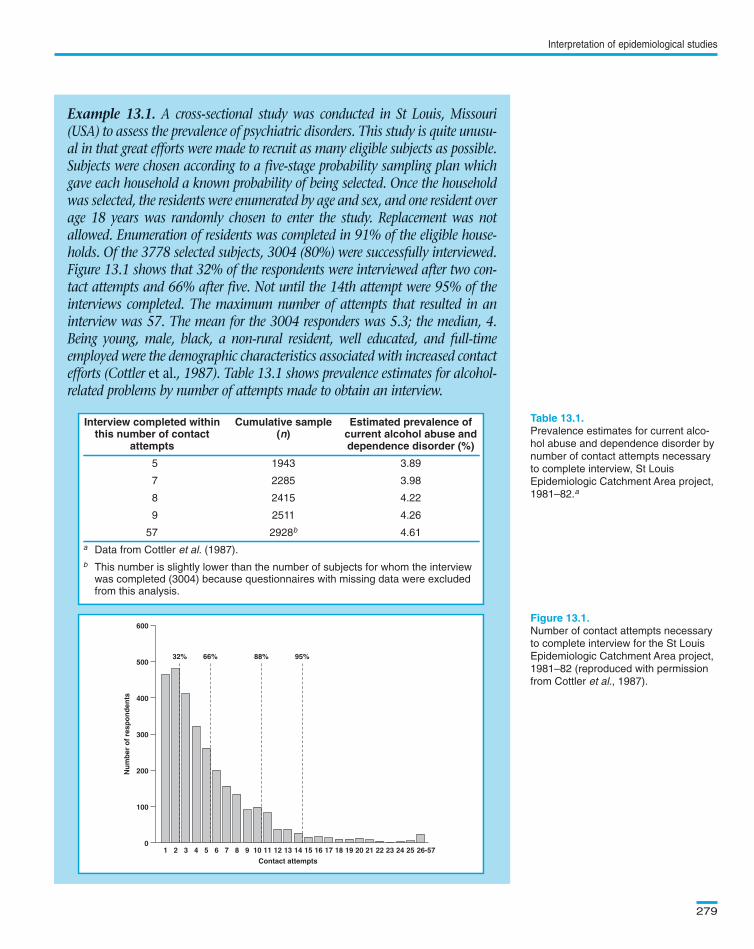
Example 13.1. A cross-sectional study was conducted in St Louis, Missouri(USA) to assess the prevalence of psychiatric disorders. This study is quite unusu-al in that great efforts were made to recruit as many eligible subjects as possible.Subjects were chosen according to a five-stage probability sampling plan whichgave each household a known probability of being selected. Once the householdwas selected, the residents were enumerated by age and sex, and one resident overage 18 years was randomly chosen to enter the study. Replacement was notallowed. Enumeration of residents was completed in 91% of the eligible house-holds. Of the 3778 selected subjects, 3004 (80%) were successfully interviewed.Figure 13.1 shows that 32% of the respondents were interviewed after two con-tact attempts and 66% after five. Not until the 14th attempt were 95% of theinterviews completed. The maximum number of attempts that resulted in aninterview was 57. The mean for the 3004 responders was 5.3; the median, 4.Being young, male, black, a non-rural resident, well educated, and full-timeemployed were the demographic characteristics associated with increased contactefforts (Cottler et al., 1987). Table 13.1 shows prevalence estimates for alcohol-related problems by number of attempts made to obtain an interview.
Interview completed within Cumulative sample Estimated prevalence ofthis number of contact (n) current alcohol abuse and
attempts dependence disorder (%)
5 1943 3.89
7 2285 3.98
8 2415 4.22
9 2511 4.26
57 2928b 4.61
a Data from Cottler et al. (1987).
b This number is slightly lower than the number of subjects for whom the interview was completed (3004) because questionnaires with missing data were excludedfrom this analysis.
Prevalence estimates for current alco-
hol abuse and dependence disorder by
number of contact attempts necessary
to complete interview, St Louis
Epidemiologic Catchment Area project,
1981–82.a
Number of contact attempts necessary
to complete interview for the St Louis
Epidemiologic Catchment Area project,
1981–82 (reproduced with permission
from Cottler et al., 1987).
01 2 3 4 5 6 7 8 9 10 11 12 13
Contact attempts
Nu
mb
er o
f re
spo
nd
ents
14 15 16 17 18 19 20 21 22 23 24 25 26-57
100
200
300
400
500
600
95%88%66%32%
Text book eng. Chap.13 final 27/05/02 10:04 Page 279 (Black/Process Black film)
Example 13.1. A cross-sectional study was conducted in St Louis, Missouri(USA) to assess the prevalence of psychiatric disorders. This study is quite unusu-al in that great efforts were made to recruit as many eligible subjects as possible.Subjects were chosen according to a five-stage probability sampling plan whichgave each household a known probability of being selected. Once the householdwas selected, the residents were enumerated by age and sex, and one resident overage 18 years was randomly chosen to enter the study. Replacement was notallowed. Enumeration of residents was completed in 91% of the eligible house-holds. Of the 3778 selected subjects, 3004 (80%) were successfully interviewed.Figure 13.1 shows that 32% of the respondents were interviewed after two con-tact attempts and 66% after five. Not until the 14th attempt were 95% of theinterviews completed. The maximum number of attempts that resulted in aninterview was 57. The mean for the 3004 responders was 5.3; the median, 4.Being young, male, black, a non-rural resident, well educated, and full-timeemployed were the demographic characteristics associated with increased contactefforts (Cottler et al., 1987). Table 13.1 shows prevalence estimates for alcohol-related problems by number of attempts made to obtain an interview.
Interview completed within Cumulative sample Estimated prevalence ofthis number of contact (n) current alcohol abuse and
attempts dependence disorder (%)
5 1943 3.89
7 2285 3.98
8 2415 4.22
9 2511 4.26
57 2928b 4.61
a Data from Cottler et al. (1987).
b This number is slightly lower than the number of subjects for whom the interviewwas completed (3004) because questionnaires with missing data were excludedfrom this analysis.
01 2 3 4 5 6 7 8 9 10 11 12 13
Contact attempts
Nu
mb
er o
f re
spo
nd
ents
14 15 16 17 18 19 20 21 22 23 24 25 26-57
100
200
300
400
500
600
95%88%66%32%
Interview completed within Cumulative sample Estimated prevalence ofthis number of contact (n) current alcohol abuse and
attempts dependence disorder (%)
5 1943 3.89
7 2285 3.98
8 2415 4.22
9 2511 4.26
57 2928b 4.61
a Data from Cottler et al. (1987).
b This number is slightly lower than the number of subjects for whom the interviewwas completed (3004) because questionnaires with missing data were excludedfrom this analysis.
Table 13.1.
Figure 13.1.
01 2 3 4 5 6 7 8 9 10 11 12 13
Contact attempts
Nu
mb
er o
f re
spo
nd
ents
14 15 16 17 18 19 20 21 22 23 24 25 26-57
100
200
300
400
500
600
95%88%66%32%
Text book eng. Chap.13 final 27/05/02 10:04 Page 279 (Black/Process Black film)TextText book book book eng. eng. eng. Chap.13 Chap.13 Chap.13 final final final 27/05/02 27/05/02 27/05/02 10:04 10:04 10:04 Page Page Page 279 279 279 (PANTONE (PANTONE (Black/Process 313 313 (Black/Process CV CV (Black/Process film) film) Black

answering the telephone numbers selected were willing to provide accurateinformation on the age and sex of all individuals living in the household.
Sometimes, it is not possible to define the population from which thecases arise. In these circumstances, hospital-based controls may be used,because the source population can then be re-defined as ‘hospital users’.Hospital controls may also be preferable for logistic reasons (easier andcheaper to identify and recruit) and because of lower potential for recallbias (see below). But selection bias may be introduced if admission to hos-pital for other conditions is related to exposure status.
shows that among men of similar age, the percentage of non-smokers was 7.0 in the hospital controls and 12.1 in the population sam-
Chapter 13
280
Example 13.2. The effect of oral contraceptive use on the risk of breast,endometrial and ovarian cancers was investigated in the Cancer and SteroidHormone Study. The study population was women aged 20–54 years whoresided in eight selected areas in the USA during the study period. Attemptswere made to identify all incident cases of breast, ovarian and endometrialcancer that occurred in the study population during the study period throughlocal population-based cancer registries. Controls were selected by random-digit dialling of households in the eight locations. A random sample of house-hold telephone numbers were called; information on the age and sex of allhousehold members was requested and controls were selected among femalemembers aged 20–54 years according to strict rules (Stadel et al., 1985).
Example 13.3. A classic case–control study was conducted in England in1948–52 to examine the relationship between cigarette smoking and lungcancer. The cases were 1488 patients admitted for lung cancer to the partic-ipating hospitals, 70% of which were located in London. A similar numberof controls were selected from patients who were admitted to the same hos-pitals with other conditions (except diseases thought at that time to be relat-ed to smoking). The smoking habits of the hospital controls were comparedwith those of a random sample of all residents in London (Table 13.2).These comparisons showed that, among men of similar ages, smoking wasmore common in the hospital controls than in the population sample (Doll& Hill, 1952).
Percentage of subjects Number (%)Subjects Most recent number of interviewed
Non- cigarettes smoked per daysmokers 1–4 5–14 15–24 25+
Hospital controls 7.0 4.2 43.3 32.1 13.4 1390 (100)
Sample of general 12.1 7.0 44.2 28.1 8.5 199 (100)population
a Data from Doll & Hill (1952).
Age-adjusted distribution of male hos-
pital controls without lung cancer and
of a random sample of men from the
general population from which the lung
cancer cases originated according to
their smoking habits.a
Text book eng. Chap.13 final 27/05/02 10:04 Page 280 (Black/Process Black film)
Table 13.2
Example 13.2. The effect of oral contraceptive use on the risk of breast,endometrial and ovarian cancers was investigated in the Cancer and SteroidHormone Study. The study population was women aged 20–54 years whoresided in eight selected areas in the USA during the study period. Attemptswere made to identify all incident cases of breast, ovarian and endometrialcancer that occurred in the study population during the study period throughlocal population-based cancer registries. Controls were selected by random-digit dialling of households in the eight locations. A random sample of house-hold telephone numbers were called; information on the age and sex of allhousehold members was requested and controls were selected among femalemembers aged 20–54 years according to strict rules (Stadel et al., 1985).
Example 13.3. A classic case–control study was conducted in England in1948–52 to examine the relationship between cigarette smoking and lungcancer. The cases were 1488 patients admitted for lung cancer to the partic-ipating hospitals, 70% of which were located in London. A similar numberof controls were selected from patients who were admitted to the same hos-pitals with other conditions (except diseases thought at that time to be relat-ed to smoking). The smoking habits of the hospital controls were comparedwith those of a random sample of all residents in London (Table 13.2).These comparisons showed that, among men of similar ages, smoking wasmore common in the hospital controls than in the population sample (Doll& Hill, 1952).
Percentage of subjects Number (%)Subjects Most recent number of interviewed
Non- cigarettes smoked per daysmokers 1–4 5–14 15–24 25+
Hospital controls 7.0 4.2 43.3 32.1 13.4 1390 (100)
Sample of general 12.1 7.0 44.2 28.1 8.5 199 (100)population
a Data from Doll & Hill (1952).
Percentage of subjects Number (%)Subjects Most recent number of interviewed
Non- cigarettes smoked per daysmokers 1–4 5–14 15–24 25+
Hospital controls 7.0 4.2 43.3 32.1 13.4 1390 (100)
Sample of general 12.1 7.0 44.2 28.1 8.5 199 (100)population
a Data from Doll & Hill (1952).
Table 13.2.
Text book eng. Chap.13 final 27/05/02 10:04 Page 280 (Black/Process Black film)TextText book book book eng. eng. eng. Chap.13 Chap.13 Chap.13 final final final 27/05/02 27/05/02 27/05/02 10:04 10:04 10:04 Page Page Page 280 280 280 (PANTONE (PANTONE (Black/Process 313 313 (Black/Process CV CV (Black/Process film) film) Black
ple. The percentage smoking at least 25 cigarettes per day was 13.4 in thehospital controls but only 8.5 in the population sample. The investigatorsstated that this difference in smoking habits between the hospital controlsand the population random sample might be explained by previouslyunknown associations between smoking and several diseases. Thus, thestrength of the association between lung cancer and cigarette smoking wasunderestimated in the case–control study, because the prevalence of smok-ing in the hospital controls was higher than in the general populationfrom which the cases of lung cancer were drawn.
A hospital control series may fail to reflect the population at riskbecause it includes people admitted to the hospital for conditions caused(or prevented) by the exposures of interest. Individuals hospitalized fordiseases related to the exposure under investigation should be excluded inorder to eliminate this type of selection bias. However, this exclusionshould not be extended to hospital patients with a history of exposure-related diseases, since no such restriction is imposed on the cases. Thus,patients admitted to hospital because of a smoking-related disorder (e.g.,chronic bronchitis) should be excluded from the control series in acase–control study looking at the relationship between smoking and lungcancer, whereas those admitted for other conditions (e.g., accidents) butwith a history of chronic bronchitis should be included.
Selection bias is less of a problem in cohort studies, because the enrol-ment of exposed and unexposed individuals is done before the develop-ment of any outcome of interest. This is also true in historical cohort stud-ies, because the ascertainment of the exposure status was made some timein the past, before the outcome was known. However, bias may still beintroduced in the selection of the ‘unexposed’ group. For instance, inoccupational cohort studies where the general population is used as thecomparison group, it is usual to find that the overall morbidity and mor-tality of the workers is lower than that of the general population. This isbecause only relatively healthy people are able to remain in employment,while the general population comprises a wider range of people includingthose who are too ill to be employed. This type of selection bias is called
Interpretation of epidemiological studies
281
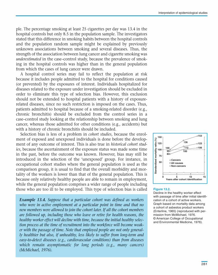
Example 13.4. Suppose that a particular cohort was defined as workerswho were in active employment at a particular point in time and that nonew members were allowed to join the cohort later. If all the cohort membersare followed up, including those who leave or retire for health reasons, thehealthy worker effect will decline with time, because the initial healthy selec-tion process at the time of recruitment into the workforce will become weak-er with the passage of time. Note that employed people are not only general-ly healthier but also, if unhealthy, less likely to suffer from long-term andeasy-to-detect diseases (e.g., cardiovascular conditions) than from diseaseswhich remain asymptomatic for long periods (e.g., many cancers)(McMichael, 1976).
Decline in the healthy worker effect
with passage of time after initial identifi-
cation of a cohort of active workers.
Graph based on mortality data among
a cohort of asbestos product workers
(Enterline, 1965) (reproduced with per-
mission from McMichael, 1976.
© American College of Occupational
and Environmental Medicine, 1976).
150
125
100
75
50
0 5Years after cohort identification
Sta
nd
ard
ized
mo
rtal
ity
rati
o (
%)
10 15
Cancers
100
112
136
1009583
106
123
153
All causesNon-cancers
Text book eng. Chap.13 final 27/05/02 10:04 Page 281 (Black/Process Black film)
Example 13.4. Suppose that a particular cohort was defined as workerswho were in active employment at a particular point in time and that nonew members were allowed to join the cohort later. If all the cohort membersare followed up, including those who leave or retire for health reasons, thehealthy worker effect will decline with time, because the initial healthy selec-tion process at the time of recruitment into the workforce will become weak-er with the passage of time. Note that employed people are not only general-ly healthier but also, if unhealthy, less likely to suffer from long-term andeasy-to-detect diseases (e.g., cardiovascular conditions) than from diseaseswhich remain asymptomatic for long periods (e.g., many cancers)(McMichael, 1976).
Figure 13.2.
150
125
100
75
50
0 5Years after cohort identification
Sta
nd
ard
ized
mo
rtal
ity
rati
o (
%)
10 15
Cancers
100
112
136
1009583
106
123
153
All causesNon-cancers
Text book eng. Chap.13 final 27/05/02 10:04 Page 281 (Black/Process Black film)TextText book book book eng. eng. eng. Chap.13 Chap.13 Chap.13 final final final 27/05/02 27/05/02 27/05/02 10:04 10:04 10:04 Page Page Page 281 281 281 (PANTONE (PANTONE (Black/Process 313 313 (Black/Process CV CV (Black/Process film) film) Black
the healthy worker effect. It may be minimized by restricting the analysis topeople from the same factory who went through the same healthy selec-tion process but have a different job (see Section 8.2.2).
shows that the healthy selection bias varies with type of dis-ease, being less marked for cancer than for non-cancer conditions (mainlycardiovascular disorders), and it tends to decline with time since recruit-ment into the workforce.
Incompleteness of follow-up due to non-response, refusal to participateand withdrawals may also be a major source of selection bias in cohort stud-ies in which people have to be followed up for long periods of time.However, this will introduce bias only if the degree of incompleteness is dif-ferent for different exposure categories. For example, subjects may be moreinclined to return for a follow-up examination if they have developed symp-toms of the disease. This tendency may be different in the exposed andunexposed, resulting in an over- or under-estimation of the effect.Definitions of individual follow-up periods may conceal this source of bias.For example, if subjects with a certain occupation tend to leave their jobwhen they develop symptoms of disease, exposed cases may not be identi-fied if follow-up terminates at the time subjects change to another job. Asimilar selection bias may occur in migrant studies if people who become illreturn to their countries of origin before their condition is properly diag-nosed in the host country.
Randomized intervention trials are less likely to be affected by selection biassince subjects are randomized to the exposure groups to be compared.However, refusals to participate after randomization and withdrawals fromthe study may affect the results if their occurrence is related to exposure sta-tus. To minimize selection bias, allocation to the various study groupsshould be conducted only after having assessed that subjects are both eligi-ble and willing to participate (see Section 7.9). The data should also beanalysed according to ‘intention to treat’ regardless of whether or not thesubjects complied with their allocated intervention (see Section 7.12).
Measurement (or information) bias occurs when measurements or classifica-tions of disease or exposure are not valid (i.e., when they do not measurecorrectly what they are supposed to measure). Errors in measurement maybe introduced by the observer (observer bias), by the study individual (respon-der bias), or by the instruments (e.g., questionnaire or sphygmomanometeror laboratory assays) used to make the measurements (see ).
Suppose that a cross-sectional survey was conducted to assess the preva-lence of a particular attribute in a certain study population. A questionnairewas administered to all eligible participants; there were no refusals. Let usdenote the observed proportion in the population classified as having the
Chapter 13
282
Text book eng. Chap.13 final 27/05/02 10:04 Page 282 (Black/Process Black film)
Example 13.4
13.1.2 Measurement bias
Chapter 2
Misclassification of a single attribute (exposure or outcome) and observedprevalence
Text book eng. Chap.13 final 27/05/02 10:04 Page 282 (Black/Process Black film)TextText book book book eng. eng. eng. Chap.13 Chap.13 Chap.13 final final final 27/05/02 27/05/02 27/05/02 10:04 10:04 10:04 Page Page Page 282 282 282 (PANTONE (PANTONE (Black/Process 313 313 (Black/Process CV CV (Black/Process film) film) Black
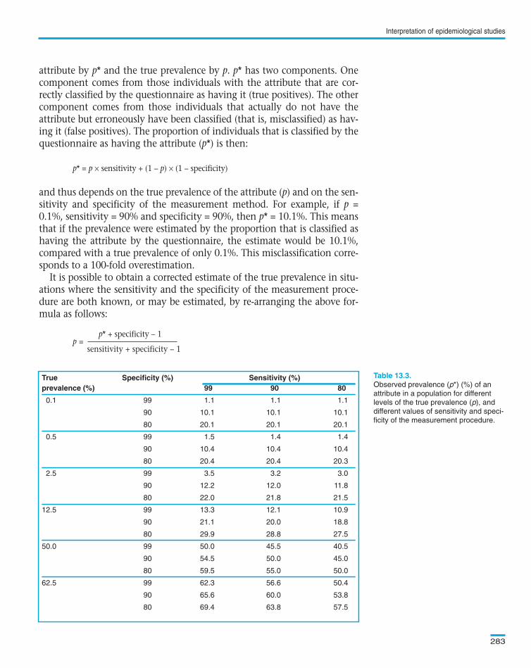
attribute by p* and the true prevalence by p. p* has two components. Onecomponent comes from those individuals with the attribute that are cor-rectly classified by the questionnaire as having it (true positives). The othercomponent comes from those individuals that actually do not have theattribute but erroneously have been classified (that is, misclassified) as hav-ing it (false positives). The proportion of individuals that is classified by thequestionnaire as having the attribute (p*) is then:
p* = p × sensitivity + (1 – p) × (1 – specificity)
and thus depends on the true prevalence of the attribute (p) and on the sen-sitivity and specificity of the measurement method. For example, if p =0.1%, sensitivity = 90% and specificity = 90%, then p* = 10.1%. This meansthat if the prevalence were estimated by the proportion that is classified ashaving the attribute by the questionnaire, the estimate would be 10.1%,compared with a true prevalence of only 0.1%. This misclassification corre-sponds to a 100-fold overestimation.
It is possible to obtain a corrected estimate of the true prevalence in situ-ations where the sensitivity and the specificity of the measurement proce-dure are both known, or may be estimated, by re-arranging the above for-mula as follows:
p* + specificity – 1p =
sensitivity + specificity – 1
Interpretation of epidemiological studies
283
True Specificity (%) Sensitivity (%)prevalence (%) 99 90 80
0.1 99 1.1 1.1 1.1
90 10.1 10.1 10.1
80 20.1 20.1 20.1
0.5 99 1.5 1.4 1.4
90 10.4 10.4 10.4
80 20.4 20.4 20.3
2.5 99 3.5 3.2 3.0
90 12.2 12.0 11.8
80 22.0 21.8 21.5
12.5 99 13.3 12.1 10.9
90 21.1 20.0 18.8
80 29.9 28.8 27.5
50.0 99 50.0 45.5 40.5
90 54.5 50.0 45.0
80 59.5 55.0 50.0
62.5 99 62.3 56.6 50.4
90 65.6 60.0 53.8
80 69.4 63.8 57.5
Observed prevalence (p*) (%) of an
attribute in a population for different
levels of the true prevalence (p), and
different values of sensitivity and speci-
ficity of the measurement procedure.
Text book eng. Chap.13 final 27/05/02 10:04 Page 283 (Black/Process Black film)
True Specificity (%) Sensitivity (%)prevalence (%) 99 90 80
0.1 99 1.1 1.1 1.1
90 10.1 10.1 10.1
80 20.1 20.1 20.1
0.5 99 1.5 1.4 1.4
90 10.4 10.4 10.4
80 20.4 20.4 20.3
2.5 99 3.5 3.2 3.0
90 12.2 12.0 11.8
80 22.0 21.8 21.5
12.5 99 13.3 12.1 10.9
90 21.1 20.0 18.8
80 29.9 28.8 27.5
50.0 99 50.0 45.5 40.5
90 54.5 50.0 45.0
80 59.5 55.0 50.0
62.5 99 62.3 56.6 50.4
90 65.6 60.0 53.8
80 69.4 63.8 57.5
Table 13.3.
Text book eng. Chap.13 final 27/05/02 10:04 Page 283 (Black/Process Black film)TextText book book book eng. eng. eng. Chap.13 Chap.13 Chap.13 final final final 27/05/02 27/05/02 27/05/02 10:04 10:04 10:04 Page Page Page 283 283 283 (PANTONE (PANTONE (Black/Process 313 313 (Black/Process CV CV (Black/Process film) film) Black
shows the effects of different levels of sensitivity and speci-ficity of a measurement procedure on the observed prevalence of a partic-ular attribute. In most cases, the observed prevalence is a gross overesti-mation of the true prevalence. For instance, the observed prevalence at90% sensitivity and 90% specificity assuming a true prevalence of 0.1% isonly about one half of that which would be obtainable if the true preva-lence were 12.5% (i.e., 10% versus 20%). The bias in overestimation isseverely influenced by losses in specificity (particularly when the trueprevalence is less than 50%). In contrast, losses in sensitivity have, atmost, moderate effects on the observed prevalence.
Two main types of misclassification may affect the interpretation ofexposure–outcome relationships: nondifferential and differential.Nondifferential misclassification occurs when an exposure or outcome clas-sification is incorrect for equal proportions of subjects in the comparedgroups. In other words, nondifferential misclassification refers to errors inclassification of outcome that are unrelated to exposure status, or misclas-sification of exposure unrelated to the individual’s outcome status. Inthese circumstances, all individuals (regardless of their exposure/outcomestatus) have the same probability of being misclassified. In contrast, differ-ential misclassification occurs when errors in classification of outcome sta-tus are dependent upon exposure status or when errors in classification ofexposure depend on outcome status.
These two types of misclassification affect results from epidemiologicalstudies in different ways. Their implications also depend on whether themisclassification relates to the exposure or the outcome status.
Nondifferential exposure misclassification occurs when all individuals(regardless of their current or future outcome status) have the same proba-bility of being misclassified in relation to their exposure status. Usually, thistype of misclassification gives rise to an underestimation of the strength ofthe association between exposure and outcome, that is, it ‘dilutes’ the effectof the exposure.
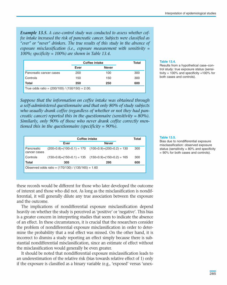
In the case–control study illustrated in , nondifferentialexposure misclassification introduced a bias towards an underestimation ofthe true exposure effect.
Nondifferential misclassification of exposure will also affect the resultsfrom studies of other types. For instance, historical occupational cohort stud-ies rely upon records of exposure of individuals from the past. However, thereoften were no specific environmental exposure measurements that wouldallow accurate classification of individuals. This means that individuals wereclassified as ‘exposed’ or ‘unexposed’ by the job they did or by membershipof a union. These proxy variables are very crude markers of the true exposurelevels and their validity is limited. It is, however, unlikely that the validity of
Chapter 13
284
Text book eng. Chap.13 final 27/05/02 10:04 Page 284 (Black/Process Black film)
Table 13.3
Misclassification and exposure–outcome relationships
Nondifferential exposure misclassification
Example 13.5
Text book eng. Chap.13 final 27/05/02 10:04 Page 284 (Black/Process Black film)TextText book book book eng. eng. eng. Chap.13 Chap.13 Chap.13 final final final 27/05/02 27/05/02 27/05/02 10:05 10:05 10:04 Page Page Page 284 284 284 (PANTONE (PANTONE (Black/Process 313 313 (Black/Process CV CV (Black/Process film) film) Black
these records would be different for those who later developed the outcomeof interest and those who did not. As long as the misclassification is nondif-ferential, it will generally dilute any true association between the exposureand the outcome.
The implications of nondifferential exposure misclassification dependheavily on whether the study is perceived as ‘positive’ or ‘negative’. This biasis a greater concern in interpreting studies that seem to indicate the absenceof an effect. In these circumstances, it is crucial that the researchers considerthe problem of nondifferential exposure misclassification in order to deter-mine the probability that a real effect was missed. On the other hand, it isincorrect to dismiss a study reporting an effect simply because there is sub-stantial nondifferential misclassification, since an estimate of effect withoutthe misclassification would generally be even greater.
It should be noted that nondifferential exposure misclassification leads toan underestimation of the relative risk (bias towards relative effect of 1) onlyif the exposure is classified as a binary variable (e.g., ‘exposed’ versus ‘unex-
Interpretation of epidemiological studies
285
Example 13.5. A case–control study was conducted to assess whether cof-fee intake increased the risk of pancreatic cancer. Subjects were classified as“ever” or “never” drinkers. The true results of this study in the absence ofexposure misclassification (i.e., exposure measurement with sensitivity =100%; specificity = 100%) are shown in Table 13.4.
Suppose that the information on coffee intake was obtained througha self-administered questionnaire and that only 80% of study subjectswho usually drank coffee (regardless of whether or not they had pan-creatic cancer) reported this in the questionnaire (sensitivity = 80%).Similarly, only 90% of those who never drank coffee correctly men-tioned this in the questionnaire (specificity = 90%).
Coffee intake Total
Ever Never
Pancreatic cancer cases 200 100 300
Controls 150 150 300
Total 350 250 600
True odds ratio = (200/100) / (150/150) = 2.00.
Results from a hypothetical case–con-
trol study: true exposure status (sensi-
tivity = 100% and specificity =100% for
both cases and controls).
Bias due to nondifferential exposure
misclassification: observed exposure
status (sensitivity = 80% and specificity
= 90% for both cases and controls).
Coffee intake TotalEver Never
Pancreatic (200×0.8)+(100×0.1) = 170 (100×0.9)+(200×0.2) = 130 300cancer cases
Controls (150×0.8)+(150×0.1) = 135 (150×0.9)+(150×0.2) = 165 300
Total 305 295 600
Observed odds ratio = (170/130) / (135/165) = 1.60
Text book eng. Chap.13 final 27/05/02 10:05 Page 285 (Black/Process Black film)
Example 13.5. A case–control study was conducted to assess whether cof-fee intake increased the risk of pancreatic cancer. Subjects were classified as“ever” or “never” drinkers. The true results of this study in the absence ofexposure misclassification (i.e., exposure measurement with sensitivity =100%; specificity = 100%) are shown in Table 13.4.
Suppose that the information on coffee intake was obtained througha self-administered questionnaire and that only 80% of study subjectswho usually drank coffee (regardless of whether or not they had pan-creatic cancer) reported this in the questionnaire (sensitivity = 80%).Similarly, only 90% of those who never drank coffee correctly men-tioned this in the questionnaire (specificity = 90%).
Coffee intake Total
Ever Never
Pancreatic cancer cases 200 100 300
Controls 150 150 300
Total 350 250 600
True odds ratio = (200/100) / (150/150) = 2.00.
Coffee intake TotalEver Never
Pancreatic (200×0.8)+(100×0.1) = 170 (100×0.9)+(200×0.2) = 130 300cancer cases
Controls (150×0.8)+(150×0.1) = 135 (150×0.9)+(150×0.2) = 165 300
Total 305 295 600
Observed odds ratio = (170/130) / (135/165) = 1.60
Coffee intake Total
Ever Never
Pancreatic cancer cases 200 100 300
Controls 150 150 300
Total 350 250 600
True odds ratio = (200/100) / (150/150) = 2.00.
Table 13.4.
Table 13.5.Coffee intake TotalEver Never
Pancreatic (200×0.8)+(100×0.1) = 170 (100×0.9)+(200×0.2) = 130 300cancer cases
Controls (150×0.8)+(150×0.1) = 135 (150×0.9)+(150×0.2) = 165 300
Total 305 295 600
Observed odds ratio = (170/130) / (135/165) = 1.60
Text book eng. Chap.13 final 27/05/02 10:05 Page 285 (Black/Process Black film)TextText book book book eng. eng. eng. Chap.13 Chap.13 Chap.13 final final final 27/05/02 27/05/02 27/05/02 10:05 10:05 10:05 Page Page Page 285 285 285 (PANTONE (PANTONE (Black/Process 313 313 (Black/Process CV CV (Black/Process film) film) Black
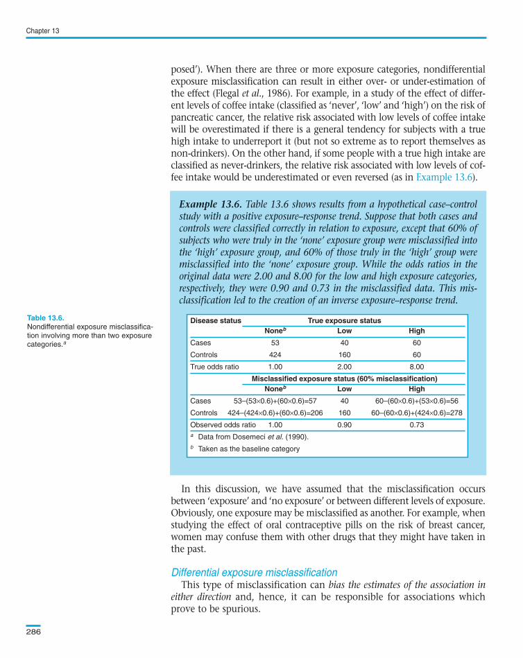
posed’). When there are three or more exposure categories, nondifferentialexposure misclassification can result in either over- or under-estimation ofthe effect (Flegal et al., 1986). For example, in a study of the effect of differ-ent levels of coffee intake (classified as ‘never’, ‘low’ and ‘high’) on the risk ofpancreatic cancer, the relative risk associated with low levels of coffee intakewill be overestimated if there is a general tendency for subjects with a truehigh intake to underreport it (but not so extreme as to report themselves asnon-drinkers). On the other hand, if some people with a true high intake areclassified as never-drinkers, the relative risk associated with low levels of cof-fee intake would be underestimated or even reversed (as in ).
In this discussion, we have assumed that the misclassification occursbetween ‘exposure’ and ‘no exposure’ or between different levels of exposure.Obviously, one exposure may be misclassified as another. For example, whenstudying the effect of oral contraceptive pills on the risk of breast cancer,women may confuse them with other drugs that they might have taken inthe past.
This type of misclassification can bias the estimates of the association ineither direction and, hence, it can be responsible for associations whichprove to be spurious.
Chapter 13
286
Example 13.6. Table 13.6 shows results from a hypothetical case–controlstudy with a positive exposure–response trend. Suppose that both cases andcontrols were classified correctly in relation to exposure, except that 60% ofsubjects who were truly in the ‘none’ exposure group were misclassified intothe ‘high’ exposure group, and 60% of those truly in the ‘high’ group weremisclassified into the ‘none’ exposure group. While the odds ratios in theoriginal data were 2.00 and 8.00 for the low and high exposure categories,respectively, they were 0.90 and 0.73 in the misclassified data. This mis-classification led to the creation of an inverse exposure–response trend.
Disease status True exposure statusNoneb Low High
Cases 53 40 60
Controls 424 160 60
True odds ratio 1.00 2.00 8.00
Misclassified exposure status (60% misclassification)Noneb Low High
Cases 53–(53×0.6)+(60×0.6)=57 40 60–(60×0.6)+(53×0.6)=56
Controls 424–(424×0.6)+(60×0.6)=206 160 60–(60×0.6)+(424×0.6)=278
Observed odds ratio 1.00 0.90 0.73
a Data from Dosemeci et al. (1990).
b Taken as the baseline category
Nondifferential exposure misclassifica-
tion involving more than two exposure
categories.a
Text book eng. Chap.13 final 27/05/02 10:05 Page 286 (Black/Process Black film)
Example 13.6
Differential exposure misclassification
Example 13.6. Table 13.6 shows results from a hypothetical case–controlstudy with a positive exposure–response trend. Suppose that both cases andcontrols were classified correctly in relation to exposure, except that 60% ofsubjects who were truly in the ‘none’ exposure group were misclassified intothe ‘high’ exposure group, and 60% of those truly in the ‘high’ group weremisclassified into the ‘none’ exposure group. While the odds ratios in theoriginal data were 2.00 and 8.00 for the low and high exposure categories,respectively, they were 0.90 and 0.73 in the misclassified data. This mis-classification led to the creation of an inverse exposure–response trend.
Disease status True exposure statusNoneb Low High
Cases 53 40 60
Controls 424 160 60
True odds ratio 1.00 2.00 8.00
Misclassified exposure status (60% misclassification)Noneb Low High
Cases 53–(53×0.6)+(60×0.6)=57 40 60–(60×0.6)+(53×0.6)=56
Controls 424–(424×0.6)+(60×0.6)=206 160 60–(60×0.6)+(424×0.6)=278
Observed odds ratio 1.00 0.90 0.73
a Data from Dosemeci et al. (1990).
b Taken as the baseline category
Table 13.6.
Text book eng. Chap.13 final 27/05/02 10:05 Page 286 (Black/Process Black film)TextText book book book eng. eng. eng. Chap.13 Chap.13 Chap.13 final final final 27/05/02 27/05/02 27/05/02 10:05 10:05 10:05 Page Page Page 286 286 286 (PANTONE (PANTONE (Black/Process 313 313 (Black/Process CV CV (Black/Process film) film) Black
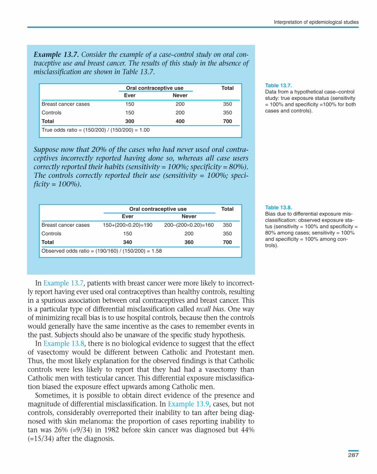
In , patients with breast cancer were more likely to incorrect-ly report having ever used oral contraceptives than healthy controls, resultingin a spurious association between oral contraceptives and breast cancer. Thisis a particular type of differential misclassification called recall bias. One wayof minimizing recall bias is to use hospital controls, because then the controlswould generally have the same incentive as the cases to remember events inthe past. Subjects should also be unaware of the specific study hypothesis.
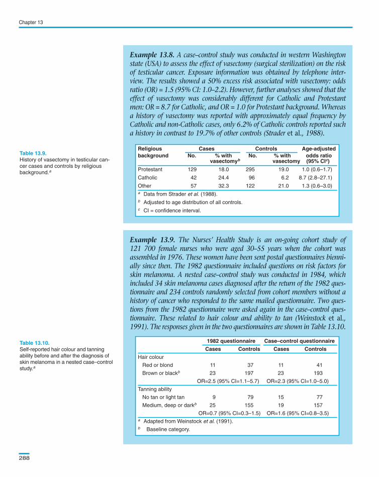
In , there is no biological evidence to suggest that the effectof vasectomy would be different between Catholic and Protestant men.Thus, the most likely explanation for the observed findings is that Catholiccontrols were less likely to report that they had had a vasectomy thanCatholic men with testicular cancer. This differential exposure misclassifica-tion biased the exposure effect upwards among Catholic men.
Sometimes, it is possible to obtain direct evidence of the presence andmagnitude of differential misclassification. In , cases, but notcontrols, considerably overreported their inability to tan after being diag-nosed with skin melanoma: the proportion of cases reporting inability totan was 26% (=9/34) in 1982 before skin cancer was diagnosed but 44%(=15/34) after the diagnosis.
Interpretation of epidemiological studies
287
Example 13.7. Consider the example of a case–control study on oral con-traceptive use and breast cancer. The results of this study in the absence ofmisclassification are shown in Table 13.7.
Suppose now that 20% of the cases who had never used oral contra-ceptives incorrectly reported having done so, whereas all case userscorrectly reported their habits (sensitivity = 100%; specificity = 80%).The controls correctly reported their use (sensitivity = 100%; speci-ficity = 100%).
Oral contraceptive use TotalEver Never
Breast cancer cases 150 200 350
Controls 150 200 350
Total 300 400 700
True odds ratio = (150/200) / (150/200) = 1.00
Data from a hypothetical case–control
study: true exposure status (sensitivity
= 100% and specificity =100% for both
cases and controls).
Bias due to differential exposure mis-
classification: observed exposure sta-
tus (sensitivity = 100% and specificity =
80% among cases; sensitivity = 100%
and specificity = 100% among con-
trols).
Oral contraceptive use TotalEver Never
Breast cancer cases 150+(200×0.20)=190 200–(200×0.20)=160 350
Controls 150 200 350
Total 340 360 700
Observed odds ratio = (190/160) / (150/200) = 1.58
Text book eng. Chap.13 final 27/05/02 10:05 Page 287 (Black/Process Black film)
Example 13.7
Example 13.8
Example 13.9
Example 13.7. Consider the example of a case–control study on oral con-traceptive use and breast cancer. The results of this study in the absence ofmisclassification are shown in Table 13.7.
Suppose now that 20% of the cases who had never used oral contra-ceptives incorrectly reported having done so, whereas all case userscorrectly reported their habits (sensitivity = 100%; specificity = 80%).The controls correctly reported their use (sensitivity = 100%; speci-ficity = 100%).
Oral contraceptive use TotalEver Never
Breast cancer cases 150 200 350
Controls 150 200 350
Total 300 400 700
True odds ratio = (150/200) / (150/200) = 1.00
Oral contraceptive use TotalEver Never
Breast cancer cases 150+(200×0.20)=190 200–(200×0.20)=160 350
Controls 150 200 350
Total 340 360 700
Observed odds ratio = (190/160) / (150/200) = 1.58
Oral contraceptive use TotalEver Never
Breast cancer cases 150 200 350
Controls 150 200 350
Total 300 400 700
True odds ratio = (150/200) / (150/200) = 1.00
Table 13.7.
Table 13.8.Oral contraceptive use TotalEver Never
Breast cancer cases 150+(200×0.20)=190 200–(200×0.20)=160 350
Controls 150 200 350
Total 340 360 700
Observed odds ratio = (190/160) / (150/200) = 1.58
Text book eng. Chap.13 final 27/05/02 10:05 Page 287 (Black/Process Black film)TextText book book book eng. eng. eng. Chap.13 Chap.13 Chap.13 final final final 27/05/02 27/05/02 27/05/02 10:05 10:05 10:05 Page Page Page 287 287 287 (PANTONE (PANTONE (Black/Process 313 313 (Black/Process CV CV (Black/Process film) film) Black
Chapter 13
288
Example 13.8. A case–control study was conducted in western Washingtonstate (USA) to assess the effect of vasectomy (surgical sterilization) on the riskof testicular cancer. Exposure information was obtained by telephone inter-view. The results showed a 50% excess risk associated with vasectomy: oddsratio (OR) = 1.5 (95% CI: 1.0–2.2). However, further analyses showed that theeffect of vasectomy was considerably different for Catholic and Protestantmen: OR = 8.7 for Catholic, and OR = 1.0 for Protestant background. Whereasa history of vasectomy was reported with approximately equal frequency byCatholic and non-Catholic cases, only 6.2% of Catholic controls reported sucha history in contrast to 19.7% of other controls (Strader et al., 1988).
History of vasectomy in testicular can-
cer cases and controls by religious
background.a
Example 13.9. The Nurses’ Health Study is an on-going cohort study of121 700 female nurses who were aged 30–55 years when the cohort wasassembled in 1976. These women have been sent postal questionnaires bienni-ally since then. The 1982 questionnaire included questions on risk factors forskin melanoma. A nested case–control study was conducted in 1984, whichincluded 34 skin melanoma cases diagnosed after the return of the 1982 ques-tionnaire and 234 controls randomly selected from cohort members without ahistory of cancer who responded to the same mailed questionnaire. Two ques-tions from the 1982 questionnaire were asked again in the case–control ques-tionnaire. These related to hair colour and ability to tan (Weinstock et al.,1991). The responses given in the two questionnaires are shown in Table 13.10.
1982 questionnaire Case–control questionnaire
Cases Controls Cases Controls
Hair colour
Red or blond 11 37 11 41
Brown or blackb 23 197 23 193
OR=2.5 (95% CI=1.1–5.7) OR=2.3 (95% CI=1.0–5.0)
Tanning ability
No tan or light tan 9 79 15 77
Medium, deep or darkb 25 155 19 157
OR=0.7 (95% CI=0.3–1.5) OR=1.6 (95% CI=0.8–3.5)
a Adapted from Weinstock et al. (1991).
b Baseline category.
Self-reported hair colour and tanning
ability before and after the diagnosis of
skin melanoma in a nested case–control
study.a
Religious Cases Controls Age-adjustedbackground No. % with No. % with odds ratio
vasectomyb vasectomy (95% CIc)
Protestant 129 18.0 295 19.0 1.0 (0.6–1.7)
Catholic 42 24.4 96 6.2 8.7 (2.8–27.1)
Other 57 32.3 122 21.0 1.3 (0.6–3.0)
a Data from Strader et al. (1988).
b Adjusted to age distribution of all controls.
c CI = confidence interval.
Text book eng. Chap.13 final 27/05/02 10:05 Page 288 (Black/Process Black film)
Example 13.8. A case–control study was conducted in western Washingtonstate (USA) to assess the effect of vasectomy (surgical sterilization) on the riskof testicular cancer. Exposure information was obtained by telephone inter-view. The results showed a 50% excess risk associated with vasectomy: oddsratio (OR) = 1.5 (95% CI: 1.0–2.2). However, further analyses showed that theeffect of vasectomy was considerably different for Catholic and Protestantmen: OR = 8.7 for Catholic, and OR = 1.0 for Protestant background. Whereasa history of vasectomy was reported with approximately equal frequency byCatholic and non-Catholic cases, only 6.2% of Catholic controls reported sucha history in contrast to 19.7% of other controls (Strader et al., 1988).
Religious Cases Controls Age-adjustedbackground No. % with No. % with odds ratio
vasectomyb vasectomy (95% CIc)
Protestant 129 18.0 295 19.0 1.0 (0.6–1.7)
Catholic 42 24.4 96 6.2 8.7 (2.8–27.1)
Other 57 32.3 122 21.0 1.3 (0.6–3.0)
a Data from Strader et al. (1988).
b Adjusted to age distribution of all controls.
c CI = confidence interval.
Table 13.9.
Example 13.9. The Nurses’ Health Study is an on-going cohort study of121 700 female nurses who were aged 30–55 years when the cohort wasassembled in 1976. These women have been sent postal questionnaires bienni-ally since then. The 1982 questionnaire included questions on risk factors forskin melanoma. A nested case–control study was conducted in 1984, whichincluded 34 skin melanoma cases diagnosed after the return of the 1982 ques-tionnaire and 234 controls randomly selected from cohort members without ahistory of cancer who responded to the same mailed questionnaire. Two ques-tions from the 1982 questionnaire were asked again in the case–control ques-tionnaire. These related to hair colour and ability to tan (Weinstock et al.,1991). The responses given in the two questionnaires are shown in Table 13.10.
1982 questionnaire Case–control questionnaire
Cases Controls Cases Controls
Hair colour
Red or blond 11 37 11 41
Brown or blackb 23 197 23 193
OR=2.5 (95% CI=1.1–5.7) OR=2.3 (95% CI=1.0–5.0)
Tanning ability
No tan or light tan 9 79 15 77
Medium, deep or darkb 25 155 19 157
OR=0.7 (95% CI=0.3–1.5) OR=1.6 (95% CI=0.8–3.5)
a Adapted from Weinstock et al. (1991).
b Baseline category.
Table 13.10.
Religious Cases Controls Age-adjustedbackground No. % with No. % with odds ratio
vasectomyb vasectomy (95% CIc)
Protestant 129 18.0 295 19.0 1.0 (0.6–1.7)
Catholic 42 24.4 96 6.2 8.7 (2.8–27.1)
Other 57 32.3 122 21.0 1.3 (0.6–3.0)
a Data from Strader et al. (1988).
b Adjusted to age distribution of all controls.
c CI = confidence interval.
Text book eng. Chap.13 final 27/05/02 10:05 Page 288 (Black/Process Black film)TextText book book book eng. eng. eng. Chap.13 Chap.13 Chap.13 final final final 27/05/02 27/05/02 27/05/02 10:05 10:05 10:05 Page Page Page 288 288 288 (PANTONE (PANTONE (Black/Process 313 313 (Black/Process CV CV (Black/Process film) film) Black
Similarly, observers who know the outcome status of an individual may beconsciously or unconsciously predisposed to assess exposure variables accord-ing to the hypothesis under study. This type of bias is known as observer bias.One way of minimizing this type of bias is to keep the observers blind to theoutcome status of the study subjects. For many diseases/conditions this isclearly impossible.
Interpretation of epidemiological studies
289
Results from a hypothetical interven-
tion trial: true outcome status (sensitiv-
ity = 100% and specificity = 100% for
both the new intervention and placebo
groups).
Bias due to nondifferential outcome
misclassification: observed outcome
status (sensitivity = 80% and specificity
= 100% for both the new intervention
and placebo groups).
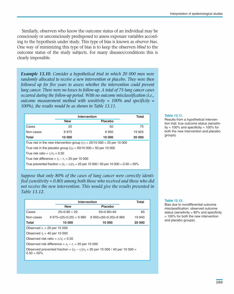
Example 13.10. Consider a hypothetical trial in which 20 000 men wererandomly allocated to receive a new intervention or placebo. They were thenfollowed up for five years to assess whether the intervention could preventlung cancer. There were no losses to follow-up. A total of 75 lung cancer casesoccurred during the follow-up period. With no outcome misclassification (i.e.,outcome measurement method with sensitivity = 100% and specificity =100%), the results would be as shown in Table 13.11.
Suppose that only 80% of the cases of lung cancer were correctly identi-fied (sensitivity = 0.80) among both those who received and those who didnot receive the new intervention. This would give the results presented inTable 13.12.
Intervention TotalNew Placebo
Cases 25 50 75
Non-cases 9 975 9 950 19 925
Total 10 000 10 000 20 000
True risk in the new intervention group (r1) = 25/10 000 = 25 per 10 000
True risk in the placebo group (r0) = 50/10 000 = 50 per 10 000
True risk ratio = r1/r0 = 0.50
True risk difference = r0 – r1 = 25 per 10 000
True prevented fraction = (r0 – r1)/r0 = 25 per 10 000 / 50 per 10 000 = 0.50 = 50%
Intervention TotalNew Placebo
Cases 25×0.80 = 20 50×0.80=40 60
Non-cases 9 975+(25×0.20) = 9 980 9 950+(50×0.20)=9 960 19 940
Total 10 000 10 000 20 000
Observed r1 = 20 per 10 000
Observed r0 = 40 per 10 000
Observed risk ratio = r1/r0 = 0.50
Observed risk difference = r0 – r1 = 20 per 10 000
Observed prevented fraction = (r0 – r1)/r0 = 20 per 10 000 / 40 per 10 000 = 0.50 = 50%
Text book eng. Chap.13 final 27/05/02 10:05 Page 289 (Black/Process Black film)
Table 13.11.
Table 13.12.
Example 13.10. Consider a hypothetical trial in which 20 000 men wererandomly allocated to receive a new intervention or placebo. They were thenfollowed up for five years to assess whether the intervention could preventlung cancer. There were no losses to follow-up. A total of 75 lung cancer casesoccurred during the follow-up period. With no outcome misclassification (i.e.,outcome measurement method with sensitivity = 100% and specificity =100%), the results would be as shown in Table 13.11.
Suppose that only 80% of the cases of lung cancer were correctly identi-fied (sensitivity = 0.80) among both those who received and those who didnot receive the new intervention. This would give the results presented inTable 13.12.
Intervention TotalNew Placebo
Cases 25 50 75
Non-cases 9 975 9 950 19 925
Total 10 000 10 000 20 000
True risk in the new intervention group (r1) = 25/10 000 = 25 per 10 000
True risk in the placebo group (r0) = 50/10 000 = 50 per 10 000
True risk ratio = r1/r0 = 0.50
True risk difference = r0 – r1 = 25 per 10 000
True prevented fraction = (r0 – r1)/r0 = 25 per 10 000 / 50 per 10 000 = 0.50 = 50%
Intervention TotalNew Placebo
Cases 25×0.80 = 20 50×0.80=40 60
Non-cases 9 975+(25×0.20) = 9 980 9 950+(50×0.20)=9 960 19 940
Total 10 000 10 000 20 000
Observed r1 = 20 per 10 000
Observed r0 = 40 per 10 000
Observed risk ratio = r1/r0 = 0.50
Observed risk difference = r0 – r1 = 20 per 10 000
Observed prevented fraction = (r0 – r1)/r0 = 20 per 10 000 / 40 per 10 000 =0.50 = 50%
Intervention TotalNew Placebo
Cases 25 50 75
Non-cases 9 975 9 950 19 925
Total 10 000 10 000 20 000
True risk in the new intervention group (r1) = 25/10 000 = 25 per 10 000
True risk in the placebo group (r0) = 50/10 000 = 50 per 10 000
True risk ratio = r1/r0 = 0.50
True risk difference = r0 – r1 = 25 per 10 000
True prevented fraction = (r0 – r1)/r0 = 25 per 10 000 / 50 per 10 000 = 0.50 = 50%
Intervention TotalNew Placebo
Cases 25×0.80 = 20 50×0.80=40 60
Non-cases 9 975+(25×0.20) = 9 980 9 950+(50×0.20)=9 960 19 940
Total 10 000 10 000 20 000
Observed r1 = 20 per 10 000
Observed r0 = 40 per 10 000
Observed risk ratio = r1/r0 = 0.50
Observed risk difference = r0 – r1 = 20 per 10 000
Observed prevented fraction = (r0 – r1)/r0 = 20 per 10 000 / 40 per 10 000 =0.50 = 50%
Text book eng. Chap.13 final 27/05/02 10:05 Page 289 (Black/Process Black film)TextText book book book eng. eng. eng. Chap.13 Chap.13 Chap.13 final final final 27/05/02 27/05/02 27/05/02 10:05 10:05 10:05 Page Page Page 289 289 289 (PANTONE (PANTONE (Black/Process 313 313 (Black/Process CV CV (Black/Process film) film) Black
Misclassification of the outcome is nondifferential if it is similar forthose exposed and those unexposed. This type of misclassification eitherdoes not affect the estimates of relative effect (if specificity = 100% andsensitivity < 100%), or it introduces a bias towards a relative effect of 1 (ifspecificity < 100% and sensitivity ≤ 100%).
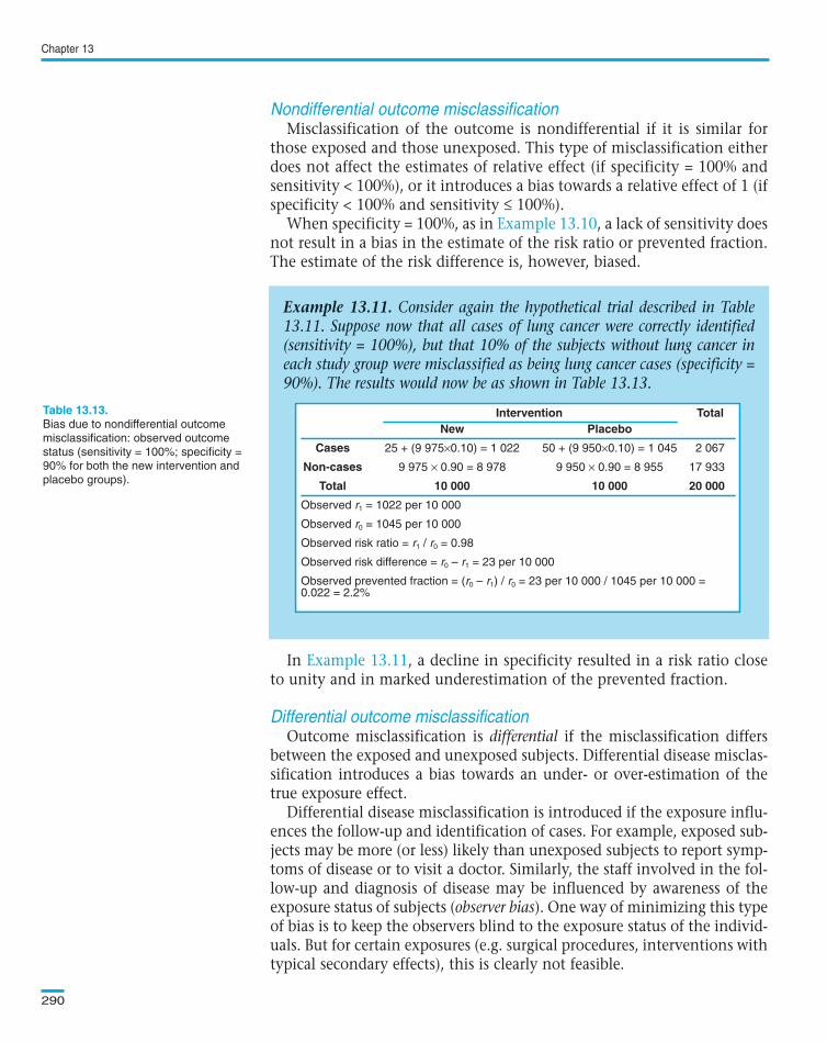
When specificity = 100%, as in , a lack of sensitivity doesnot result in a bias in the estimate of the risk ratio or prevented fraction.The estimate of the risk difference is, however, biased.
In , a decline in specificity resulted in a risk ratio closeto unity and in marked underestimation of the prevented fraction.
Outcome misclassification is differential if the misclassification differsbetween the exposed and unexposed subjects. Differential disease misclas-sification introduces a bias towards an under- or over-estimation of thetrue exposure effect.
Differential disease misclassification is introduced if the exposure influ-ences the follow-up and identification of cases. For example, exposed sub-jects may be more (or less) likely than unexposed subjects to report symp-toms of disease or to visit a doctor. Similarly, the staff involved in the fol-low-up and diagnosis of disease may be influenced by awareness of theexposure status of subjects (observer bias). One way of minimizing this typeof bias is to keep the observers blind to the exposure status of the individ-uals. But for certain exposures (e.g. surgical procedures, interventions withtypical secondary effects), this is clearly not feasible.
Chapter 13
290
Example 13.11. Consider again the hypothetical trial described in Table13.11. Suppose now that all cases of lung cancer were correctly identified(sensitivity = 100%), but that 10% of the subjects without lung cancer ineach study group were misclassified as being lung cancer cases (specificity =90%). The results would now be as shown in Table 13.13.
Bias due to nondifferential outcome
misclassification: observed outcome
status (sensitivity = 100%; specificity =
90% for both the new intervention and
placebo groups).
Intervention TotalNew Placebo
Cases 25 + (9 975×0.10) = 1 022 50 + (9 950×0.10) = 1 045 2 067
Non-cases 9 975 × 0.90 = 8 978 9 950 × 0.90 = 8 955 17 933
Total 10 000 10 000 20 000
Observed r1 = 1022 per 10 000
Observed r0 = 1045 per 10 000
Observed risk ratio = r1 / r0 = 0.98
Observed risk difference = r0 – r1 = 23 per 10 000
Observed prevented fraction = (r0 – r1) / r0 = 23 per 10 000 / 1045 per 10 000 = 0.022 = 2.2%
Text book eng. Chap.13 final 27/05/02 10:05 Page 290 (Black/Process Black film)
Nondifferential outcome misclassification
Example 13.10
Example 13.11
Differential outcome misclassification
Example 13.11. Consider again the hypothetical trial described in Table13.11. Suppose now that all cases of lung cancer were correctly identified(sensitivity = 100%), but that 10% of the subjects without lung cancer ineach study group were misclassified as being lung cancer cases (specificity =90%). The results would now be as shown in Table 13.13.
Intervention TotalNew Placebo
Cases 25 + (9 975×0.10) = 1 022 50 + (9 950×0.10) = 1 045 2 067
Non-cases 9 975 × 0.90 = 8 978 9 950 × 0.90 = 8 955 17 933
Total 10 000 10 000 20 000
Observed r1 = 1022 per 10 000
Observed r0 = 1045 per 10 000
Observed risk ratio = r1 / r0 = 0.98
Observed risk difference = r0 – r1 = 23 per 10 000
Observed prevented fraction = (r0 – r1) / r0 = 23 per 10 000 / 1045 per 10 000 =0.022 = 2.2%
Table 13.13. Intervention TotalNew Placebo
Cases 25 + (9 975×0.10) = 1 022 50 + (9 950×0.10) = 1 045 2 067
Non-cases 9 975 × 0.90 = 8 978 9 950 × 0.90 = 8 955 17 933
Total 10 000 10 000 20 000
Observed r1 = 1022 per 10 000
Observed r0 = 1045 per 10 000
Observed risk ratio = r1 / r0 = 0.98
Observed risk difference = r0 – r1 = 23 per 10 000
Observed prevented fraction = (r0 – r1) / r0 = 23 per 10 000 / 1045 per 10 000 =0.022 = 2.2%
Text book eng. Chap.13 final 27/05/02 10:05 Page 290 (Black/Process Black film)TextText book book book eng. eng. eng. Chap.13 Chap.13 Chap.13 final final final 27/05/02 27/05/02 27/05/02 10:05 10:05 10:05 Page Page Page 290 290 290 (PANTONE (PANTONE (Black/Process 313 313 (Black/Process CV CV (Black/Process film) film) Black
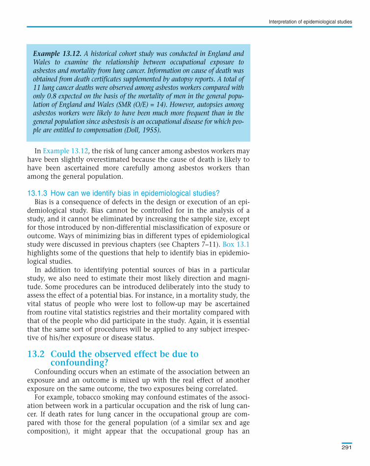
In , the risk of lung cancer among asbestos workers mayhave been slightly overestimated because the cause of death is likely tohave been ascertained more carefully among asbestos workers thanamong the general population.
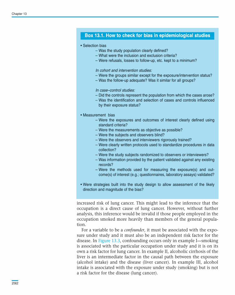
Bias is a consequence of defects in the design or execution of an epi-demiological study. Bias cannot be controlled for in the analysis of astudy, and it cannot be eliminated by increasing the sample size, exceptfor those introduced by non-differential misclassification of exposure oroutcome. Ways of minimizing bias in different types of epidemiologicalstudy were discussed in previous chapters (see Chapters 7–11). highlights some of the questions that help to identify bias in epidemio-logical studies.
In addition to identifying potential sources of bias in a particularstudy, we also need to estimate their most likely direction and magni-tude. Some procedures can be introduced deliberately into the study toassess the effect of a potential bias. For instance, in a mortality study, thevital status of people who were lost to follow-up may be ascertainedfrom routine vital statistics registries and their mortality compared withthat of the people who did participate in the study. Again, it is essentialthat the same sort of procedures will be applied to any subject irrespec-tive of his/her exposure or disease status.
Confounding occurs when an estimate of the association between anexposure and an outcome is mixed up with the real effect of anotherexposure on the same outcome, the two exposures being correlated.
For example, tobacco smoking may confound estimates of the associ-ation between work in a particular occupation and the risk of lung can-cer. If death rates for lung cancer in the occupational group are com-pared with those for the general population (of a similar sex and agecomposition), it might appear that the occupational group has an
Interpretation of epidemiological studies
291
Example 13.12. A historical cohort study was conducted in England andWales to examine the relationship between occupational exposure toasbestos and mortality from lung cancer. Information on cause of death wasobtained from death certificates supplemented by autopsy reports. A total of11 lung cancer deaths were observed among asbestos workers compared withonly 0.8 expected on the basis of the mortality of men in the general popu-lation of England and Wales (SMR (O/E) = 14). However, autopsies amongasbestos workers were likely to have been much more frequent than in thegeneral population since asbestosis is an occupational disease for which peo-ple are entitled to compensation (Doll, 1955).
Text book eng. Chap.13 final 27/05/02 10:05 Page 291 (Black/Process Black film)
Example 13.12
13.1.3 How can we identify bias in epidemiological studies?
Box 13.1
13.2 Could the observed effect be due to confounding?
Example 13.12. A historical cohort study was conducted in England andWales to examine the relationship between occupational exposure toasbestos and mortality from lung cancer. Information on cause of death wasobtained from death certificates supplemented by autopsy reports. A total of11 lung cancer deaths were observed among asbestos workers compared withonly 0.8 expected on the basis of the mortality of men in the general popu-lation of England and Wales (SMR (O/E) = 14). However, autopsies amongasbestos workers were likely to have been much more frequent than in thegeneral population since asbestosis is an occupational disease for which peo-ple are entitled to compensation (Doll, 1955).
Text book eng. Chap.13 final 27/05/02 10:05 Page 291 (Black/Process Black film)TextText book book book eng. eng. eng. Chap.13 Chap.13 Chap.13 final final final 27/05/02 27/05/02 27/05/02 10:05 10:05 10:05 Page Page Page 291 291 291 (PANTONE (PANTONE (Black/Process 313 313 (Black/Process CV CV (Black/Process film) film) Black
increased risk of lung cancer. This might lead to the inference that theoccupation is a direct cause of lung cancer. However, without furtheranalysis, this inference would be invalid if those people employed in theoccupation smoked more heavily than members of the general popula-tion.
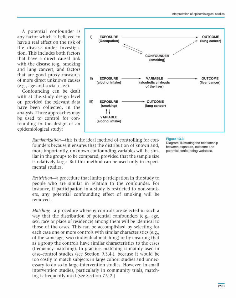
For a variable to be a confounder, it must be associated with the expo-sure under study and it must also be an independent risk factor for thedisease. In , confounding occurs only in example I—smokingis associated with the particular occupation under study and it is on itsown a risk factor for lung cancer. In example II, alcoholic cirrhosis of theliver is an intermediate factor in the causal path between the exposure(alcohol intake) and the disease (liver cancer). In example III, alcoholintake is associated with the exposure under study (smoking) but is nota risk factor for the disease (lung cancer).
Chapter 13
292
Box 13.1. How to check for bias in epidemiological studies
• Selection bias
– Was the study population clearly defined?
– What were the inclusion and exclusion criteria?
– Were refusals, losses to follow-up, etc. kept to a minimum?
In cohort and intervention studies:
– Were the groups similar except for the exposure/intervention status?
– Was the follow-up adequate? Was it similar for all groups?
In case–control studies:
– Did the controls represent the population from which the cases arose?
– Was the identification and selection of cases and controls influenced
by their exposure status?
• Measurement bias
– Were the exposures and outcomes of interest clearly defined using
standard criteria?
– Were the measurements as objective as possible?
– Were the subjects and observers blind?
– Were the observers and interviewers rigorously trained?
– Were clearly written protocols used to standardize procedures in data
collection?
– Were the study subjects randomized to observers or interviewers?
– Was information provided by the patient validated against any existing
records?
– Were the methods used for measuring the exposure(s) and out-
come(s) of interest (e.g.; questionnaires, laboratory assays) validated?
• Were strategies built into the study design to allow assessment of the likely
direction and magnitude of the bias?
Text book eng. Chap.13 final 27/05/02 10:05 Page 292 (Black/Process Black film)
Figure 13.3
Box 13.1. How to check for bias in epidemiological studies
• Selection bias
– Was the study population clearly defined?
– What were the inclusion and exclusion criteria?
– Were refusals, losses to follow-up, etc. kept to a minimum?
In cohort and intervention studies:
– Were the groups similar except for the exposure/intervention status?
– Was the follow-up adequate? Was it similar for all groups?
In case–control studies:
– Did the controls represent the population from which the cases arose?
– Was the identification and selection of cases and controls influenced
by their exposure status?
• Measurement bias
– Were the exposures and outcomes of interest clearly defined using
standard criteria?
– Were the measurements as objective as possible?
– Were the subjects and observers blind?
– Were the observers and interviewers rigorously trained?
– Were clearly written protocols used to standardize procedures in data
collection?
– Were the study subjects randomized to observers or interviewers?
– Was information provided by the patient validated against any existing
records?
– Were the methods used for measuring the exposure(s) and out-
come(s) of interest (e.g.; questionnaires, laboratory assays) validated?
• Were strategies built into the study design to allow assessment of the likely
direction and magnitude of the bias?
Box 13.1. How to check for bias in epidemiological studiesBox 13.1. How to check for bias in epidemiological studiesBoxBox 13.1. 13.1. How How to to check check for for bias bias in in epidemiological epidemiological studies studies
Text book eng. Chap.13 final 27/05/02 10:05 Page 292 (Black/Process Black film)TextText book book book eng. eng. eng. Chap.13 Chap.13 Chap.13 final final final 27/05/02 27/05/02 27/05/02 10:05 10:05 10:05 Page Page Page 292 292 292 (PANTONE (PANTONE (Black/Process 313 313 (Black/Process CV CV (Black/Process film) film) Black
A potential confounder isany factor which is believed tohave a real effect on the risk ofthe disease under investiga-tion. This includes both factorsthat have a direct causal linkwith the disease (e.g., smokingand lung cancer), and factorsthat are good proxy measuresof more direct unknown causes(e.g., age and social class).
Confounding can be dealtwith at the study design levelor, provided the relevant datahave been collected, in theanalysis. Three approaches maybe used to control for con-founding in the design of anepidemiological study:
Randomization—this is the ideal method of controlling for con-founders because it ensures that the distribution of known and,more importantly, unknown confounding variables will be sim-ilar in the groups to be compared, provided that the sample sizeis relatively large. But this method can be used only in experi-mental studies.
Restriction—a procedure that limits participation in the study topeople who are similar in relation to the confounder. Forinstance, if participation in a study is restricted to non-smok-ers, any potential confounding effect of smoking will beremoved.
Matching—a procedure whereby controls are selected in such away that the distribution of potential confounders (e.g., age,sex, race or place of residence) among them will be identical tothose of the cases. This can be accomplished by selecting foreach case one or more controls with similar characteristics (e.g.,of the same age, sex) (individual matching) or by ensuring thatas a group the controls have similar characteristics to the cases(frequency matching). In practice, matching is mainly used incase–control studies (see Section 9.3.4.), because it would betoo costly to match subjects in large cohort studies and unnec-essary to do so in large intervention studies. However, in smallintervention studies, particularly in community trials, match-ing is frequently used (see Section 7.9.2.)
Interpretation of epidemiological studies
293
EXPOSURE(Occupation)
I)
II)
III)
EXPOSURE(alcohol intake)
EXPOSURE(smoking)
VARIABLE(alcohol intake)
VARIABLE(alcoholic cirrhosis
of the liver)
OUTCOME(liver cancer)
OUTCOME(lung cancer)
CONFOUNDER(smoking)
OUTCOME(lung cancer)
Diagram illustrating the relationship
between exposure, outcome and
potential confounding variables.
Text book eng. Chap.13 final 27/05/02 10:05 Page 293 (Black/Process Black film)
EXPOSURE(Occupation)
I)
II)
III)
EXPOSURE(alcohol intake)
EXPOSURE(smoking)
VARIABLE(alcohol intake)
VARIABLE(alcoholic cirrhosis
of the liver)
OUTCOME(liver cancer)
OUTCOME(lung cancer)
CONFOUNDER(smoking)
OUTCOME(lung cancer)
Figure 13.3.
Text book eng. Chap.13 final 27/05/02 10:05 Page 293 (Black/Process Black film)TextText book book book eng. eng. eng. Chap.13 Chap.13 Chap.13 final final final 27/05/02 27/05/02 27/05/02 10:05 10:05 10:05 Page Page Page 293 293 293 (PANTONE (PANTONE (Black/Process 313 313 (Black/Process CV CV (Black/Process film) film) Black
Confounding can also be controlled for in the analysis by using:
Stratification—a technique in which the strength of the associationis measured separately within each well defined and homogeneouscategory (stratum) of the confounding variable. For instance, if ageis a confounder, the association is estimated separately in eachage-group; the results can then be pooled using a suitable weight-ing to obtain an overall summary measure of the association,which is adjusted or controlled for the effects of the confounder(that is, that takes into account differences between the groups inthe distribution of confounders; see Chapter 14). It should benoted that standardization, a technique mentioned in Chapter 4,is an example of stratification.
Statistical modelling—sophisticated statistical methods, such asregression modelling, are available to control for confounding.They are particularly useful when it is necessary to adjust simulta-neously for various confounders. These techniques are brieflyintroduced in Chapter 14.
It is possible to control for confounders in the analysis only if data onthem were collected; the extent to which confounding can be controlledfor will depend on the accuracy of these data. For instance, nondifferen-tial (random) misclassification of exposure to a confounder will lead tounderestimation of the effect of the confounder and consequently, willattenuate the degree to which confounding can be controlled. The associ-ation will persist even after the adjustment because of residual confounding.But in contrast to non-differential misclassification of exposure or outcome,non-differential misclassification of a confounder will cause a bias in eitherdirection, depending on the direction of the confounding. For example, ina study of risk factors for cervical cancer, the association between cigarettesmoking and cervical cancer persisted even after controlling in the analy-sis for the number of sexual partners. This might be due, at least in part,to residual confounding because ‘number of sexual partners’ is an inaccu-rate measure of sexual behaviour, including infection by human papillo-mavirus.
The assessment of the role of chance in the interpretation of resultsfrom epidemiological studies was discussed in Chapter 6. In summary, therole of chance can be assessed by performing appropriate statistical signif-icance tests and by calculating confidence intervals.
A statistical significance test for the effect of an exposure on an outcomeyields the probability (P or P-value) that a result as extreme as or moreextreme than the one observed could have occurred by chance alone, i.e.,if there were no true relationship between the exposure and the outcome.
Chapter 13
294
Text book eng. Chap.13 final 27/05/02 10:05 Page 294 (Black/Process Black film)
13.3 Could the observed effect be due to chance?
Text book eng. Chap.13 final 27/05/02 10:05 Page 294 (Black/Process Black film)TextText book book book eng. eng. eng. Chap.13 Chap.13 Chap.13 final final final 27/05/02 27/05/02 27/05/02 10:05 10:05 10:05 Page Page Page 294 294 294 (PANTONE (PANTONE (Black/Process 313 313 (Black/Process CV CV (Black/Process film) film) Black
If this probability is very small, it is usual to declare that chance is anunlikely explanation for the observed association and consequently, thatthere is a ‘statistically significant’ association between exposure and out-come. If the P-value is large (usually greater than 0.05), it is conventional-ly thought that chance cannot be excluded as an explanation for theobserved association.
A number of issues should be kept in mind when interpreting resultsfrom statistical tests. Firstly, the value of P depends both on the magnitudeof the association and on the study size. It is therefore possible with smallstudies to obtain a P-value which is not statistically significant, despite thefact that the true population exposure effect is large. Conversely, with alarge sample, small effects, which may be clinically and epidemiologicallyirrelevant, may easily achieve statistical significance. Confidence intervalsare more informative than P-values because they provide a range of valuesfor the exposure–outcome association, which is likely to include the truepopulation effect (usually with a probability of 0.95, i.e. 95%). They alsoindicate whether a non-significant result is or is not compatible with atrue effect that was not detected because the sample size was too small (seeChapter 6). Sample size calculations should always be done at the designstage to ensure that the study will have enough power (i.e., its sample sizewill be large enough) to detect the hypothetical effect or enough precisionto quantify it (see Chapter 15).
Secondly, investigators tend to collect data on many potential risk fac-tors and to perform multiple statistical tests to determine whether any ofthese variables is significantly associated with the disease or outcome ofinterest. However, the probability of obtaining a statistically significant P-value just by chance increases with the number of tests performed. It isparticularly important to keep this in mind when the data are interpreted,particularly if an unexpected association is found that was not hypothe-sized at the beginning of the study. Such an unexpected association wouldhave to be reproduced in studies specifically designed to test it before itcould be accepted as real.
Finally, statistical methods assess only the effects of sampling variationand cannot control for non-sampling errors such as confounding or biasin the design, conduct or analysis of a study.
If bias, confounding and chance do not seem to explain an observedassociation, can we conclude that the association is likely to be causal?Since we can never be sure that the study was not affected by any of thesefactors, we need to consider the findings in the context of all available evi-dence. In a paper published in 1965, Bradford Hill mentioned aspects thatneed to considered when assessing whether an association is likely to becausal (Hill, 1965). We will consider each of these aspects below. As anillustration, we show how these aspects were applied to evaluate the asso-ciation between smoking and lung cancer.
Interpretation of epidemiological studies
295
Text book eng. Chap.13 final 27/05/02 10:05 Page 295 (Black/Process Black film)
13.4 Could the observed effect be causal?
Text book eng. Chap.13 final 27/05/02 10:05 Page 295 (Black/Process Black film)TextText book book book eng. eng. eng. Chap.13 Chap.13 Chap.13 final final final 27/05/02 27/05/02 27/05/02 10:05 10:05 10:05 Page Page Page 295 295 295 (PANTONE (PANTONE (Black/Process 313 313 (Black/Process CV CV (Black/Process film) film) Black
This is an essential aspect. For an exposure to be the cause of a dis-ease, it has to precede its biological onset. This is generally easier toestablish from intervention or cohort studies than from cross-section-al or case–control studies in which measurements of the exposure andthe outcome are made at the same time.
“The criterion of temporality requires that cigarette smoking ante-date the onset of cancer. Support for this criterion is provided by allthe major prospective [cohort] studies in which an enormous num-ber of initially disease-free subjects were followed over varying timeintervals.” (US Surgeon General, 1982)
The association is more likely to be causal if consistent with otherbiological knowledge (e.g., animal experiments, biological mecha-nisms). However, this aspect should not be taken too seriously, becauselack of plausibility may simply reflect lack of scientific knowledge orthe fact that human beings are biologically different from animals.
“Benign and malignant tumours have been induced in the larynxof hamsters by long-term exposure to diluted cigarette smoke.Attempts to induce significant numbers of bronchogenic carcino-ma [lung cancer] in laboratory animals were negative in spite ofmajor efforts with several species and strains. Neither rats nor ham-sters nor baboons inhale cigarette smoke as deeply and as intense-ly as the cigarette smokers who have provided the data with theconsequences of their ‘experiment’ in the form of clinical evidencegathered by epidemiologists.” (US Surgeon General, 1982)
If similar results have been found in different populations using dif-ferent study designs, the association is more likely to be causal, sinceit is unlikely that all studies were subject to the same type of biasand/or confounding. However, a lack of consistency does not excludea causal association, since different intensity levels and other condi-tions may reduce the impact of the exposure in certain studies.
“More than 50 retrospective [case–control] studies have reportedsmoking patterns (by type and quantity of tobacco smoked, dura-tion of smoking, and inhalational practice) in a variety of subjectswith lung cancer (e.g., males and females, different occupationalgroups, hospitalized patients, autopsy cases, all individuals whodied from lung cancer in an area, nationwide sample of individualswho died from lung cancer, and different races and ethnic groups).
Chapter 13
296
Text book eng. Chap.13 final 27/05/02 10:05 Page 296 (Black/Process Black film)
Temporal relationship
Biological plausibility
Consistency
Text book eng. Chap.13 final 27/05/02 10:05 Page 296 (Black/Process Black film)TextText book book book eng. eng. eng. Chap.13 Chap.13 Chap.13 final final final 27/05/02 27/05/02 27/05/02 10:05 10:05 10:05 Page Page Page 296 296 296 (PANTONE (PANTONE (Black/Process 313 313 (Black/Process CV CV (Black/Process film) film) Black
Many of these subjects have been compared with matched controlsalso drawn from a variety of groups (e.g., healthy individuals,patients hospitalized for cancer or other diseases, deaths from can-cers of other sites, and samplings of the general population).Regardless of the method, these studies have consistently found anassociation between smoking and lung cancer. Relative risks forsmokers are consistently greater than for nonsmokers. ( … ) Eight major prospective [cohort] studies have examined the rela-tionship between smoking and lung cancer mortality in a largenumber of subjects, in different countries, and in different timeperiods. The results of these studies ( … ) are consistent with eachother as well as with the retrospective [case–control] studies.” (USSurgeon General, 1982)
The strength of an association is measured by the magnitude of therelative measure of effect. A strong association is not easily explainedby potential sources of bias or confounding and hence it is more like-ly to be causal than is a weak association, which could more easily bethe result of confounding or bias. For example, a relative risk of mag-nitude 10 is more likely to reflect a true causal association than one of1.5.
“Prospective [cohort] studies have shown that the death rate fromlung cancer among cigarette smokers is approximately 10 times therate in non-smokers ( … ). To account for such a high relative riskin terms of an indirect association would require that an unknowncausal factor be present at least 10 times more frequently amongsmokers ( … ) than among non-smokers. Such a confounding fac-tor should be easily detectable, and if it cannot be detected or rea-sonably inferred, the finding of such a strong association makes aconclusion concerning causality more probable.” (US SurgeonGeneral, 1982)
Further evidence of a causal relationship is provided if increasinglevels of exposure are associated with increasing incidence of disease.
“The strongest exposure-relationship measured in most epidemio-logical studies was for the number of cigarettes smoked per day atthe time of entry into the study. However, other important mea-sures of dosage include the age at which smoking began, the dura-tion of smoking, and inhalation practice. ( … ) The data ( … ) indi-cate that as the number of cigarettes smoked per day increases thereis a gradient of risk for lung cancer mortality. ( … ) Male smokerswho smoked more than 20 cigarettes daily had lung cancer mortal-
Interpretation of epidemiological studies
297
Text book eng. Chap.13 final 27/05/02 10:05 Page 297 (Black/Process Black film)
Strength
Exposure–response relationship
Text book eng. Chap.13 final 27/05/02 10:05 Page 297 (Black/Process Black film)TextText book book book eng. eng. eng. Chap.13 Chap.13 Chap.13 final final final 27/05/02 27/05/02 27/05/02 10:05 10:05 10:05 Page Page Page 297 297 297 (PANTONE (PANTONE (Black/Process 313 313 (Black/Process CV CV (Black/Process film) film) Black
ity ratios 15 to 25 times greater than nonsmokers. Similar findingswere observed among female smokers ( … ).
Four prospective [cohort] studies which examined lung cancermortality by age began smoking ( … ) show a strong inverse rela-tionship ( … ), i.e., the younger the age one began smoking, thegreater the lung cancer mortality rate.” (US Surgeon General, 1982)
If a particular exposure increases the risk of a certain disease but notthe risk of other diseases, this provides evidence in favour of acause–effect relationship. However, one-to-one relationships betweenexposure and disease are rare and lack of specificity should not be usedto refute a causal relationship.
“Tobacco smoke is a complex mixture consisting of several thou-sand chemical substances. These diverse substances are capable ofproducing more than a single biological response. The specificity ofthe association between smoking and lung cancer is evidenced bycomparison of the magnitude of lung cancer mortality ratios tothose of other cancers, as has been done in most of the prospective[cohort] studies. The mortality ratios for lung cancer are very highwhen compared with those of other cancers.” (US Surgeon General,1982)
When the removal of a possible cause results in a reduced incidenceof the disease, the likelihood of the association being causal isstrengthened. Ideally, this should be assessed by conducting a ran-domized intervention trial, but for many exposures–disease associa-tions, such randomized trials are impossible in practice.
“Since cigarette smoking is significantly associated with lung can-cer, it is logical to expect that cessation of smoking would lead to adecrease in mortality rates from lung cancer among quitters com-pared to persons who continue to smoke cigarettes. In fact, all ofthe major studies which examined cessation showed this decreasein lung cancer risk. ( … ) After 15 to 20 years, the ex-smoker’s riskof dying from lung cancer gradually decreases to a point where itmore closely approximates the risk of the non-smoker ( … ). Themagnitude of the residual risk that ex-smokers experience is large-ly determined by the cumulative exposure to tobacco prior tosmoking cessation (i.e., total amount the individual smoked, agewhen smoking began, and degree of inhalation), and varies withnumber of years since quitting smoking, as well as with the reasonsfor quitting smoking (e.g., quitting due to symptoms of disease).”(US Surgeon General, 1982)
Chapter 13
298
Text book eng. Chap.13 final 27/05/02 10:05 Page 298 (Black/Process Black film)
Specificity
Reversibility
Text book eng. Chap.13 final 27/05/02 10:05 Page 298 (Black/Process Black film)TextText book book book eng. eng. eng. Chap.13 Chap.13 Chap.13 final final final 27/05/02 27/05/02 27/05/02 10:05 10:05 10:05 Page Page Page 298 298 298 (PANTONE (PANTONE (Black/Process 313 313 (Black/Process CV CV (Black/Process film) film) Black
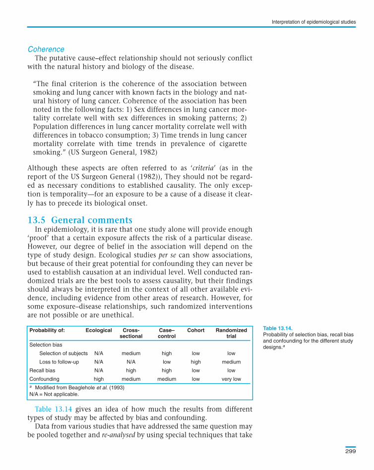
The putative cause–effect relationship should not seriously conflictwith the natural history and biology of the disease.
“The final criterion is the coherence of the association betweensmoking and lung cancer with known facts in the biology and nat-ural history of lung cancer. Coherence of the association has beennoted in the following facts: 1) Sex differences in lung cancer mor-tality correlate well with sex differences in smoking patterns; 2)Population differences in lung cancer mortality correlate well withdifferences in tobacco consumption; 3) Time trends in lung cancermortality correlate with time trends in prevalence of cigarettesmoking.” (US Surgeon General, 1982)
Although these aspects are often referred to as ‘criteria’ (as in thereport of the US Surgeon General (1982)), They should not be regard-ed as necessary conditions to established causality. The only excep-tion is temporality—for an exposure to be a cause of a disease it clear-ly has to precede its biological onset.
In epidemiology, it is rare that one study alone will provide enough‘proof’ that a certain exposure affects the risk of a particular disease.However, our degree of belief in the association will depend on thetype of study design. Ecological studies per se can show associations,but because of their great potential for confounding they can never beused to establish causation at an individual level. Well conducted ran-domized trials are the best tools to assess causality, but their findingsshould always be interpreted in the context of all other available evi-dence, including evidence from other areas of research. However, forsome exposure–disease relationships, such randomized interventionsare not possible or are unethical.
gives an idea of how much the results from differenttypes of study may be affected by bias and confounding.
Data from various studies that have addressed the same question maybe pooled together and re-analysed by using special techniques that take
Interpretation of epidemiological studies
299
Probability of selection bias, recall bias
and confounding for the different study
designs.a
Probability of: Ecological Cross- Case– Cohort Randomizedsectional control trial
Selection bias
Selection of subjects N/A medium high low low
Loss to follow-up N/A N/A low high medium
Recall bias N/A high high low low
Confounding high medium medium low very low
a Modified from Beaglehole et al. (1993)
N/A = Not applicable.
Text book eng. Chap.13 final 27/05/02 10:05 Page 299 (Black/Process Black film)
Coherence
13.5 General comments
Table 13.14
Table 13.14.Probability of: Ecological Cross- Case– Cohort Randomizedsectional control trial
Selection bias
Selection of subjects N/A medium high low low
Loss to follow-up N/A N/A low high medium
Recall bias N/A high high low low
Confounding high medium medium low very low
a Modified from Beaglehole et al. (1993)
N/A = Not applicable.
Text book eng. Chap.13 final 27/05/02 10:05 Page 299 (Black/Process Black film)TextText book book book eng. eng. eng. Chap.13 Chap.13 Chap.13 final final final 27/05/02 27/05/02 27/05/02 10:05 10:05 10:05 Page Page Page 299 299 299 (PANTONE (PANTONE (Black/Process 313 313 (Black/Process CV CV (Black/Process film) film) Black
into account the fact that the original studies may differ in a large num-ber of respects (e.g., characteristics of the study subjects, methods ofdata collection). This approach is particularly useful when the effect ofthe exposure is likely to be small, so that a very large sample size will benecessary to detect and quantify it precisely (as in ).
Meta-analysis is another technique used to combine results from var-ious studies. It differs from a re-analysis in that there is no access to theraw data from each individual study. Only the published estimates ofexposure effect from each study are available and can be used to gener-ate a pooled overall result.
It is essential to ensure that practically all studies (published andunpublished) are included in any re-analysis or meta-analysis. This isbecause published studies tend to be a biased sample with an overrep-resentation of those which showed ‘positive’ findings.
Chapter 13
300
Example 13.13. A large number of cohort and case–control studies were con-ducted in recent decades to examine the relationship of oral contraceptive useand breast cancer. Their results were largely inconsistent. To clarify this issue,data from most of these studies were brought together and re-analysed. The54 studies included in this re-analysis were conducted in 25 countries inEurope, North America, Asia, Australasia, Africa and Latin America.Together they included 53 297 women with invasive breast cancer and100 239 without breast cancer. Figure 13.4 shows relative risks of breast can-cer in ever-users versus never-users of combined oral contraceptives (the mostwidely used type). The risk estimates varied substantially from study to study,but most confidence intervals were wide and included the null hypothesisvalue of 1. The pooled estimate was slightly above 1 (1.07) and its confi-dence interval did not include the null hypothesis value. Current users of com-bined oral contraceptives or those who stopped less than 10 years previouslyappeared to have a small increase in the risk of having breast cancer diag-nosed relative to never-users, but this excess in risk disappeared 10 or moreyears after stopping use (Figure 13.5d) (Collaborative Group on HormonalFactors in Breast Cancer, 1996).
Text book eng. Chap.13 final 27/05/02 10:05 Page 300 (Black/Process Black film)
Example 13.13
Example 13.13. A large number of cohort and case–control studies were con-ducted in recent decades to examine the relationship of oral contraceptive useand breast cancer. Their results were largely inconsistent. To clarify this issue,data from most of these studies were brought together and re-analysed. The54 studies included in this re-analysis were conducted in 25 countries inEurope, North America, Asia, Australasia, Africa and Latin America.Together they included 53 297 women with invasive breast cancer and100 239 without breast cancer. Figure 13.4 shows relative risks of breast can-cer in ever-users versus never-users of combined oral contraceptives (the mostwidely used type). The risk estimates varied substantially from study to study,but most confidence intervals were wide and included the null hypothesisvalue of 1. The pooled estimate was slightly above 1 (1.07) and its confi-dence interval did not include the null hypothesis value. Current users of com-bined oral contraceptives or those who stopped less than 10 years previouslyappeared to have a small increase in the risk of having breast cancer diag-nosed relative to never-users, but this excess in risk disappeared 10 or moreyears after stopping use (Figure 13.5d) (Collaborative Group on HormonalFactors in Breast Cancer, 1996).
Text book eng. Chap.13 final 27/05/02 10:05 Page 300 (Black/Process Black film)TextText book book book eng. eng. eng. Chap.13 Chap.13 Chap.13 final final final 27/05/02 27/05/02 27/05/02 10:05 10:05 10:05 Page Page Page 300 300 300 (PANTONE (PANTONE (Black/Process 313 313 (Black/Process CV CV (Black/Process film) film) Black
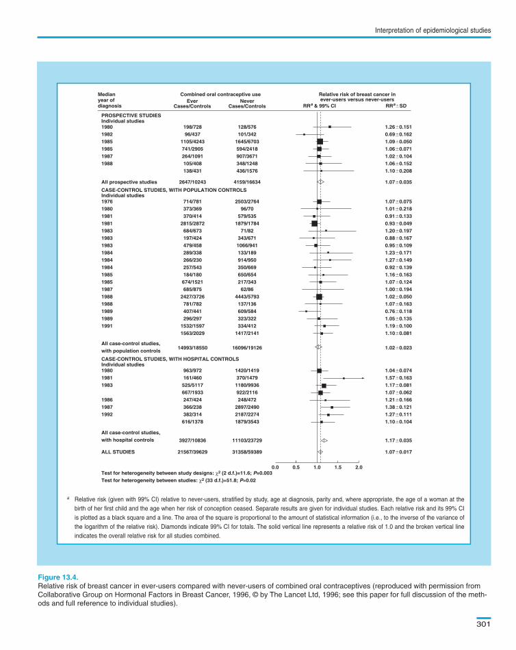
Interpretation of epidemiological studies
301
Relative risk of breast cancer in ever-users compared with never-users of combined oral contraceptives (reproduced with permission from
Collaborative Group on Hormonal Factors in Breast Cancer, 1996, © by The Lancet Ltd, 1996; see this paper for full discussion of the meth-
ods and full reference to individual studies).
Medianyear ofdiagnosis
198019821985198519871988
PROSPECTIVE STUDIES
198/72896/437
1105/4243741/2905264/1091105/408138/431
128/576101/342
1645/6703594/2418907/3671348/1248436/1576
1.26�0.1510.69�0.1621.09�0.0501.06�0.0711.02�0.1041.06�0.1521.10�0.208
All prospective studies
Individual studies
Individual studies
2647/10243 4159/16634 1.07�0.035
197619801981198119831983198319841984198419851985198719881988198919891991
CASE-CONTROL STUDIES, WITH POPULATION CONTROLS
714/781373/369370/414
2815/2872684/673197/424479/458289/338266/230257/543184/180674/1521685/875
2427/3726781/782407/441296/297
1532/15971563/2029
2503/276496/70
579/5351879/1784
71/82343/6711066/941133/189914/950350/669650/654217/34362/86
4443/5793137/136609/584323/322334/412
1417/2141
1.07�0.0751.01�0.2180.91�0.1330.93�0.0491.20�0.1970.88�0.1670.95�0.1091.23�0.1711.27�0.1490.92�0.1391.16�0.1631.07�0.1241.00�0.1941.02�0.0501.07�0.1630.76�0.1181.05�0.1351.19�0.1001.10�0.081
All case-control studies,with population controls
14993/18550 16096/19126 1.02�0.023
ALL STUDIES
All case-control studies,with hospital controls
Individual studies
Test for heterogeneity between study designs: χ2 (2 d.f.)=11.6; P=0.003Test for heterogeneity between studies: χ2 (33 d.f.)=51.8; P=0.02
3927/10836 11103/23729
21567/39629 31358/59389
0.0 0.5 1.0 1.5 2.0
1.17�0.035
1.07�0.017
198019811983
198619871992
CASE-CONTROL STUDIES, WITH HOSPITAL CONTROLS
963/972161/460525/5117667/1933247/424366/238382/314616/1378
1420/1419370/14791180/9936922/2116248/472
2897/24902187/22741879/3543
1.04�0.0741.57�0.1631.17�0.0811.07�0.0621.21�0.1661.38�0.1211.27�0.1111.10�0.104
Combined oral contraceptive use Relative risk of breast cancer inever-users versus never-usersEver
Cases/ControlsNever
Cases/Controls RRa & 99% CI RRa�SD
a Relative risk (given with 99% CI) relative to never-users, stratified by study, age at diagnosis, parity and, where appropriate, the age of a woman at the
birth of her first child and the age when her risk of conception ceased. Separate results are given for individual studies. Each relative risk and its 99% CI
is plotted as a black square and a line. The area of the square is proportional to the amount of statistical information (i.e., to the inverse of the variance of
the logarithm of the relative risk). Diamonds indicate 99% CI for totals. The solid vertical line represents a relative risk of 1.0 and the broken vertical line
indicates the overall relative risk for all studies combined.
Text book eng. Chap.13 final 27/05/02 10:05 Page 301 (Black/Process Black film)
Medianyear ofdiagnosis
198019821985198519871988
PROSPECTIVE STUDIES
198/72896/437
1105/4243741/2905264/1091105/408138/431
128/576101/342
1645/6703594/2418907/3671348/1248436/1576
1.26�0.1510.69�0.1621.09�0.0501.06�0.0711.02�0.1041.06�0.1521.10�0.208
All prospective studies
Individual studies
Individual studies
2647/10243 4159/16634 1.07�0.035
197619801981198119831983198319841984198419851985198719881988198919891991
CASE-CONTROL STUDIES, WITH POPULATION CONTROLS
714/781373/369370/414
2815/2872684/673197/424479/458289/338266/230257/543184/180674/1521685/875
2427/3726781/782407/441296/297
1532/15971563/2029
2503/276496/70
579/5351879/1784
71/82343/6711066/941133/189914/950350/669650/654217/34362/86
4443/5793137/136609/584323/322334/412
1417/2141
1.07�0.0751.01�0.2180.91�0.1330.93�0.0491.20�0.1970.88�0.1670.95�0.1091.23�0.1711.27�0.1490.92�0.1391.16�0.1631.07�0.1241.00�0.1941.02�0.0501.07�0.1630.76�0.1181.05�0.1351.19�0.1001.10�0.081
All case-control studies,with population controls
14993/18550 16096/19126 1.02�0.023
ALL STUDIES
All case-control studies,with hospital controls
Individual studies
Test for heterogeneity between study designs: χ2 (2 d.f.)=11.6; P=0.003Test for heterogeneity between studies: χ2 (33 d.f.)=51.8; P=0.02
3927/10836 11103/23729
21567/39629 31358/59389
0.0 0.5 1.0 1.5 2.0
1.17�0.035
1.07�0.017
198019811983
198619871992
CASE-CONTROL STUDIES, WITH HOSPITAL CONTROLS
963/972161/460525/5117667/1933247/424366/238382/314616/1378
1420/1419370/14791180/9936922/2116248/472
2897/24902187/22741879/3543
1.04�0.0741.57�0.1631.17�0.0811.07�0.0621.21�0.1661.38�0.1211.27�0.1111.10�0.104
Combined oral contraceptive use Relative risk of breast cancer inever-users versus never-usersEver
Cases/ControlsNever
Cases/Controls RRa & 99% CI RRa�SD
a Relative risk (given with 99% CI) relative to never-users, stratified by study, age at diagnosis, parity and, where appropriate, the age of a woman at the
birth of her first child and the age when her risk of conception ceased. Separate results are given for individual studies. Each relative risk and its 99% CI
is plotted as a black square and a line. The area of the square is proportional to the amount of statistical information (i.e., to the inverse of the variance of
the logarithm of the relative risk). Diamonds indicate 99% CI for totals. The solid vertical line represents a relative risk of 1.0 and the broken vertical line
indicates the overall relative risk for all studies combined.
Figure 13.4.
Medianyear ofdiagnosis
198019821985198519871988
PROSPECTIVE STUDIES
198/72896/437
1105/4243741/2905264/1091105/408138/431
128/576101/342
1645/6703594/2418907/3671348/1248436/1576
1.26�0.1510.69�0.1621.09�0.0501.06�0.0711.02�0.1041.06�0.1521.10�0.208
All prospective studies
Individual studies
Individual studies
2647/10243 4159/16634 1.07�0.035
197619801981198119831983198319841984198419851985198719881988198919891991
CASE-CONTROL STUDIES, WITH POPULATION CONTROLS
714/781373/369370/414
2815/2872684/673197/424479/458289/338266/230257/543184/180674/1521685/875
2427/3726781/782407/441296/297
1532/15971563/2029
2503/276496/70
579/5351879/1784
71/82343/6711066/941133/189914/950350/669650/654217/34362/86
4443/5793137/136609/584323/322334/412
1417/2141
1.07�0.0751.01�0.2180.91�0.1330.93�0.0491.20�0.1970.88�0.1670.95�0.1091.23�0.1711.27�0.1490.92�0.1391.16�0.1631.07�0.1241.00�0.1941.02�0.0501.07�0.1630.76�0.1181.05�0.1351.19�0.1001.10�0.081
All case-control studies,with population controls
14993/18550 16096/19126 1.02�0.023
ALL STUDIES
All case-control studies,with hospital controls
Individual studies
Test for heterogeneity between study designs: χ2 (2 d.f.)=11.6; P=0.003Test for heterogeneity between studies: χ2 (33 d.f.)=51.8; P=0.02
3927/10836 11103/23729
21567/39629 31358/59389
0.0 0.5 1.0 1.5 2.0
1.17�0.035
1.07�0.017
198019811983
198619871992
CASE-CONTROL STUDIES, WITH HOSPITAL CONTROLS
963/972161/460525/5117667/1933247/424366/238382/314616/1378
1420/1419370/14791180/9936922/2116248/472
2897/24902187/22741879/3543
1.04�0.0741.57�0.1631.17�0.0811.07�0.0621.21�0.1661.38�0.1211.27�0.1111.10�0.104
Combined oral contraceptive use Relative risk of breast cancer inever-users versus never-usersEver
Cases/ControlsNever
Cases/Controls RRa & 99% CI RRa�SD
a Relative risk (given with 99% CI) relative to never-users, stratified by study, age at diagnosis, parity and, where appropriate, the age of a woman at the
birth of her first child and the age when her risk of conception ceased. Separate results are given for individual studies. Each relative risk and its 99% CI
is plotted as a black square and a line. The area of the square is proportional to the amount of statistical information (i.e., to the inverse of the variance of
the logarithm of the relative risk). Diamonds indicate 99% CI for totals. The solid vertical line represents a relative risk of 1.0 and the broken vertical line
indicates the overall relative risk for all studies combined.
Text book eng. Chap.13 final 27/05/02 10:05 Page 301 (Black/Process Black film)TextText book book book eng. eng. eng. Chap.13 Chap.13 Chap.13 final final final 27/05/02 27/05/02 27/05/02 10:05 10:05 10:05 Page Page Page 301 301 301 (PANTONE (PANTONE (Black/Process 313 313 (Black/Process CV CV (Black/Process film) film) Black
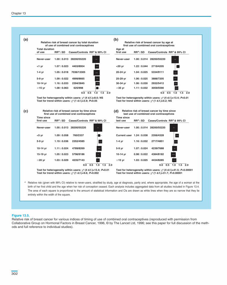
Chapter 13
302
Relative risk of breast cancer by total durationof use of combined oral contraceptives
Total durationof use
Test for heterogeneity within users: χ2 (4 d.f.)=8.0; NSTest for trend within users: χ2 (1 d.f.)=3.9; P=0.05
Never-user
RRa�SD Cases/Controls
1.00�0.013 28200/55220
<1 yr 1.07�0.023 4403/8954
1-4 yr 1.05�0.018 7036/13305
5-9 yr 1.09�0.022 4999/8665
10-14 yr 1.16�0.033 2394/3845
�15 yr 1.08�0.063 625/998
RRa & 99% CI
0.0 0.5 1.0 1.5 2.0
Relative risk of breast cancer by age at first use of combined oral contraceptives
Age at first use
Test for heterogeneity within users: χ2 (4 d.f.)=13.4; P=0.01Test for trend within users: χ2 (1 d.f.)=0.2; NS
Never-user
RRa�SD Cases/Controls
1.00�0.014 28200/55220
<20 yr 1.22�0.044 2719/4205
20-24 yr 1.04�0.025 5334/9111
25-29 yr 1.06�0.025 3888/7205
30-34 yr 1.06�0.030 2932/5412
�35 yr 1.11�0.032 3059/5590
RRa & 99% CI
0.0 0.5 1.0 1.5 2.0
Relative risk of breast cancer by time sincefirst use of combined oral contraceptives
Time sincefirst use
Test for heterogeneity within users: χ2 (4 d.f.)=13.4; P=0.01Test for trend within users: χ2 (1 d.f.)=9.6; P=0.002
Never-user
RRa�SD Cases/Controls
1.00�0.013 28200/55220
<5 yr 1.09�0.058 760/2337
5-9 yr 1.19�0.036 2352/4585
10-14 yr 1.11�0.024 4789/8269
15-19 yr 1.05�0.023 5796/9186
�20 yr 1.03�0.029 4235/7143
RRa & 99% CI
0.0 0.5 1.0 1.5 2.0
Relative risk of breast cancer by time since last use of combined oral contraceptives
Time sincelast use
Test for heterogeneity within users: χ2 (4 d.f.)=41.5; P<0.00001Test for trend within users: χ2 (1 d.f.)=31.7; P<0.00001
Never-user
RRa�SD Cases/Controls
1.00�0.014 28200/55220
Current user 1.24�0.038 2356/4328
1-4 yr 1.16�0.032 2717/4851
5-9 yr 1.07�0.024 4239/7688
10-14 yr 0.98�0.022 4384/8182
�15 yr 1.03�0.025 4434/8285
RRa & 99% CI
0.0 0.5 1.0 1.5 2.0
a Relative risk (given with 99% CI) relative to never-users, stratified by study, age at diagnosis, parity and, where appropriate, the age of a woman at the
birth of her first child and the age when her risk of conception ceased. Each analysis includes aggregated data from all studies included in Figure 13.4.
The area of each square is proportional to the amount of statistical information and CIs are drawn as white lines when they are so narrow that they lie
entirely within the width of the square.
Relative risk of breast cancer for various indices of timing of use of combined oral contraceptives (reproduced with permission from
Collaborative Group on Hormonal Factors in Breast Cancer, 1996, © by The Lancet Ltd, 1996; see this paper for full discussion of the meth-
ods and full reference to individual studies).
(a) (b)
(c) (d)
Text book eng. Chap.13 final 27/05/02 10:05 Page 302 (Black/Process Black film)
Relative risk of breast cancer by total durationof use of combined oral contraceptives
Total durationof use
Test for heterogeneity within users: χ2 (4 d.f.)=8.0; NSTest for trend within users: χ2 (1 d.f.)=3.9; P=0.05
Never-user
RRa�SD Cases/Controls
1.00�0.013 28200/55220
<1 yr 1.07�0.023 4403/8954
1-4 yr 1.05�0.018 7036/13305
5-9 yr 1.09�0.022 4999/8665
10-14 yr 1.16�0.033 2394/3845
�15 yr 1.08�0.063 625/998
RRa & 99% CI
0.0 0.5 1.0 1.5 2.0
Relative risk of breast cancer by age atfirst use of combined oral contraceptives
Age atfirst use
Test for heterogeneity within users: χ2 (4 d.f.)=13.4; P=0.01Test for trend within users: χ2 (1 d.f.)=0.2; NS
Never-user
RRa�SD Cases/Controls
1.00�0.014 28200/55220
<20 yr 1.22�0.044 2719/4205
20-24 yr 1.04�0.025 5334/9111
25-29 yr 1.06�0.025 3888/7205
30-34 yr 1.06�0.030 2932/5412
�35 yr 1.11�0.032 3059/5590
RRa & 99% CI
0.0 0.5 1.0 1.5 2.0
Relative risk of breast cancer by time sincefirst use of combined oral contraceptives
Time sincefirst use
Test for heterogeneity within users: χ2 (4 d.f.)=13.4; P=0.01Test for trend within users: χ2 (1 d.f.)=9.6; P=0.002
Never-user
RRa�SD Cases/Controls
1.00�0.013 28200/55220
<5 yr 1.09�0.058 760/2337
5-9 yr 1.19�0.036 2352/4585
10-14 yr 1.11�0.024 4789/8269
15-19 yr 1.05�0.023 5796/9186
�20 yr 1.03�0.029 4235/7143
RRa & 99% CI
0.0 0.5 1.0 1.5 2.0
Relative risk of breast cancer by time sincelast use of combined oral contraceptives
Time sincelast use
Test for heterogeneity within users: χ2 (4 d.f.)=41.5; P<0.00001Test for trend within users: χ2 (1 d.f.)=31.7; P<0.00001
Never-user
RRa�SD Cases/Controls
1.00�0.014 28200/55220
Current user 1.24�0.038 2356/4328
1-4 yr 1.16�0.032 2717/4851
5-9 yr 1.07�0.024 4239/7688
10-14 yr 0.98�0.022 4384/8182
�15 yr 1.03�0.025 4434/8285
RRa & 99% CI
0.0 0.5 1.0 1.5 2.0
a Relative risk (given with 99% CI) relative to never-users, stratified by study, age at diagnosis, parity and, where appropriate, the age of a woman at the
birth of her first child and the age when her risk of conception ceased. Each analysis includes aggregated data from all studies included in Figure 13.4.
The area of each square is proportional to the amount of statistical information and CIs are drawn as white lines when they are so narrow that they lie
entirely within the width of the square.
(a) (b)
(c) (d)
Figure 13.5.
(b)
(d)
Text book eng. Chap.13 final 27/05/02 10:05 Page 302 (Black/Process Black film)TextText book book book eng. eng. eng. Chap.13 Chap.13 Chap.13 final final final 27/05/02 27/05/02 27/05/02 10:05 10:05 10:05 Page Page Page 302 302 302 (PANTONE (PANTONE (Black/Process 313 313 (Black/Process CV CV (Black/Process film) film) Black
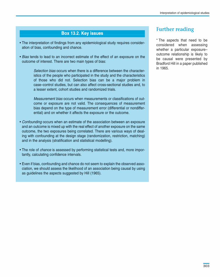
Interpretation of epidemiological studies
303
* The aspects that need to be
considered when assessing
whether a particular exposure–
outcome relationship is likely to
be causal were presented by
Bradford Hill in a paper published
in 1965.
Box 13.2. Key issues
• The interpretation of findings from any epidemiological study requires consider-
ation of bias, confounding and chance.
• Bias tends to lead to an incorrect estimate of the effect of an exposure on the
outcome of interest. There are two main types of bias:
Selection bias occurs when there is a difference between the character-
istics of the people who participated in the study and the characteristics
of those who did not. Selection bias can be a major problem in
case–control studies, but can also affect cross-sectional studies and, to
a lesser extent, cohort studies and randomized trials.
Measurement bias occurs when measurements or classifications of out-
come or exposure are not valid. The consequences of measurement
bias depend on the type of measurement error (differential or nondiffer-
ential) and on whether it affects the exposure or the outcome.
• Confounding occurs when an estimate of the association between an exposure
and an outcome is mixed up with the real effect of another exposure on the same
outcome, the two exposures being correlated. There are various ways of deal-
ing with confounding at the design stage (randomization, restriction, matching)
and in the analysis (stratification and statistical modelling).
• The role of chance is assessed by performing statistical tests and, more impor-
tantly, calculating confidence intervals.
• Even if bias, confounding and chance do not seem to explain the observed asso-
ciation, we should assess the likelihood of an association being causal by using
as guidelines the aspects suggested by Hill (1965).
Text book eng. Chap.13 final 27/05/02 10:05 Page 303 (Black/Process Black film)
Further readingBox 13.2. Key issues
• The interpretation of findings from any epidemiological study requires consider-
ation of bias, confounding and chance.
• Bias tends to lead to an incorrect estimate of the effect of an exposure on the
outcome of interest. There are two main types of bias:
Selection bias occurs when there is a difference between the character-
istics of the people who participated in the study and the characteristics
of those who did not. Selection bias can be a major problem in
case–control studies, but can also affect cross-sectional studies and, to
a lesser extent, cohort studies and randomized trials.
Measurement bias occurs when measurements or classifications of out-
come or exposure are not valid. The consequences of measurement
bias depend on the type of measurement error (differential or nondiffer-
ential) and on whether it affects the exposure or the outcome.
• Confounding occurs when an estimate of the association between an exposure
and an outcome is mixed up with the real effect of another exposure on the same
outcome, the two exposures being correlated. There are various ways of deal-
ing with confounding at the design stage (randomization, restriction, matching)
and in the analysis (stratification and statistical modelling).
• The role of chance is assessed by performing statistical tests and, more impor-
tantly, calculating confidence intervals.
• Even if bias, confounding and chance do not seem to explain the observed asso-
ciation, we should assess the likelihood of an association being causal by using
as guidelines the aspects suggested by Hill (1965).
Box 13.2. Key issuesBox 13.2. Key issuesBoxBox 13.2. 13.2. Key Key issues issues
Text book eng. Chap.13 final 27/05/02 10:05 Page 303 (Black/Process Black film)TextText book book book eng. eng. eng. Chap.13 Chap.13 Chap.13 final final final 27/05/02 27/05/02 27/05/02 10:05 10:05 10:05 Page Page Page 303 303 303 (PANTONE (PANTONE (Black/Process 313 313 (Black/Process CV CV (Black/Process film) film) Black