Interpolating CurvesD.A. Forsyth UIUC

Central issues in modelling

• Construct families of curves, surfaces and volumes that• can represent common objects usefully;• are easy to interact with; interaction includes:

• manual modelling;• fitting to measurements;

• support geometric computations• intersection• collision

• Question: How much do you know about B-Splines?

Main topics

• Simple curves• Interpolation• Continuity and splines for interpolation

Parametric forms

• A parametric curve is • a mapping of one parameter into

• 2D• 3D

• Examples• circle as (cos t, sin t)• twisted cubic as (t, t*t, t*t*t)• circle as (1-t^2, 2 t, 0)/(1+t^2)

• domain of the parametrization MATTERS• (cos t, sin t), 0<=t<= pi is a semicircle

Curves - basic ideas

• Important cases on the plane• Monge (or explicit)

• y(x)• Examples:

• many lines, bits of circle, sines, etc• Implicit curve

• F(x, y)=0• Examples:

• all lines, circles, ellipses• any explicit curve; any parametric algebraic curve; lots of others• Important special case: F polynomial

• Parametric curve• (x(s), y(s)) for s in some range• Examples

• all lines, circles, ellipses• Important special cases: x, y polynomials, rational

Powerful view of a curve

• A set of points pasted together by blending functions• blending functions depend on parameter• points (control points; control vectors) don’t• representation isn’t unique (but that really doesn’t matter very much)

• Advantage:• we don’t need to worry much about dimension

• that’s carried by the points• we can do a variety of clever tricks with the blending functions

• meet constraints• convert from form to form

p0�0(t) + p1�1(t) + v0�2(t) + v1�3(t)

Interpolation

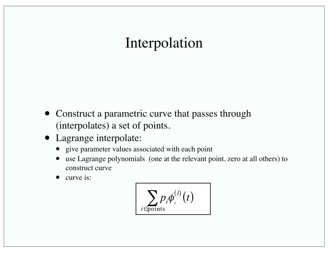
• Construct a parametric curve that passes through (interpolates) a set of points.

• Lagrange interpolate:• give parameter values associated with each point• use Lagrange polynomials (one at the relevant point, zero at all others) to

construct curve• curve is:

piφ i

l( ) t( )i∈points∑

Lagrange interpolate

• Construct a parametric curve that passes through (interpolates) a set of points.

• Lagrange interpolate:• give parameter values associated with each point• use Lagrange polynomials (one at the relevant point, zero at all others) to

construct curve• degree is (#pts-1)

• e.g. line through two points• quadratic through three.

•

Lagrange polynomials

• Interpolate points at s=s_i, i=1..n• Blending functions

• Can do this with a polynomial

�i(s) =

⇢1 s = si0 s = sk, k 6= i

Qj=1..i�1,i..n(s� sj)Qj=1..i�1,i..n(sj � si)

Hermite interpolation

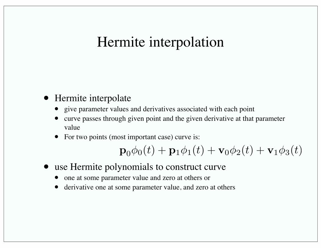
• Hermite interpolate• give parameter values and derivatives associated with each point• curve passes through given point and the given derivative at that parameter

value• For two points (most important case) curve is:

• use Hermite polynomials to construct curve• one at some parameter value and zero at others or• derivative one at some parameter value, and zero at others

p0�0(t) + p1�1(t) + v0�2(t) + v1�3(t)

Hermite curves

• Natural matrix form:• solve linear system to get curve coefficients

• Easily “pasted” together

Blending functions are cubic polynomials, so we write as:

This allows us to write the curve as:

Basis matrix Geometry matrix

p0�0(t) + p1�1(t) + v0�2(t) + v1�3(t)

⇥�0(t) �1(t) �2(t) �3(t)

⇤=

⇥1 t t2 t3

⇤

8>><

>>:

a0 a1 a2 a3b0 b1 b2 b3c0 c1 c2 c3d0 d1 d2 d3

9>>=

>>;

⇥1 t t2 t3

⇤

8>><

>>:

a0 a1 a2 a3b0 b1 b2 b3c0 c1 c2 c3d0 d1 d2 d3

9>>=

>>;

8>><

>>:

p0

p1

v0

v1

9>>=

>>;

Hermite polynomials

⇥�0(t) �1(t) �2(t) �3(t)

⇤=

⇥1 t t2 t3

⇤

8>><

>>:

a0 a1 a2 a3b0 b1 b2 b3c0 c1 c2 c3d0 d1 d2 d3

9>>=

>>;

d

dt

⇥�0(t) �1(t) �2(t) �3(t)

⇤=

⇥0 1 2t 3t2

⇤

8>><

>>:

a0 a1 a2 a3b0 b1 b2 b3c0 c1 c2 c3d0 d1 d2 d3

9>>=

>>;

Constraints

These constraints give:

Interpolate each endpoint Have correct derivatives at each endpoint

2

664

�0(0) �1(0) �2(0) �3(0)�0(1) �1(1) �2(1) �3(1)d�0

dt (0)d�1

dt (0)d�2

dt (0)d�3

dt (0)d�0

dt (1)d�1

dt (1)d�2

dt (1)d�3

dt (1)

3

775 =

2

664

1 0 0 00 1 0 00 0 1 00 0 0 1

3

775

We can write individual constraints like:

To get:

⇥�0(0) �1(0) �2(0) �3(0)

⇤=

⇥1 0 02 03

⇤

8>><

>>:

a0 a1 a2 a3b0 b1 b2 b3c0 c1 c2 c3d0 d1 d2 d3

9>>=

>>;

2

664

1 0 0 01 1 1 10 1 0 00 1 2 3

3

775

8>><

>>:

a0 a1 a2 a3b0 b1 b2 b3c0 c1 c2 c3d0 d1 d2 d3

9>>=

>>;=

2

664

1 0 0 00 1 0 00 0 1 00 0 0 1

3

775

Hermite blending functions

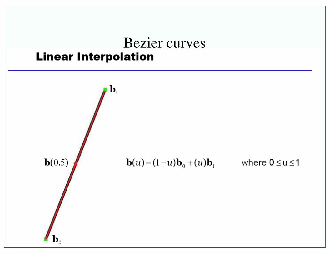
Bezier curves

Bezier curves

Bezier curves

Bezier curves as a tableau

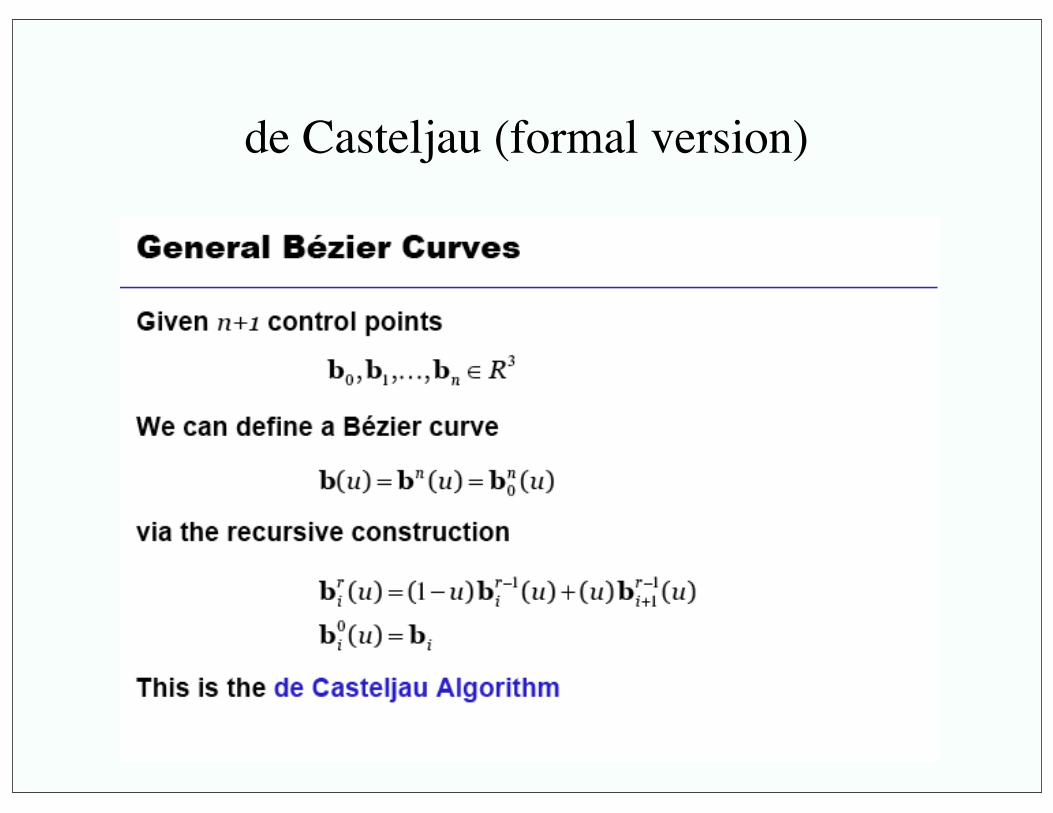
de Casteljau (formal version)

Bezier curve blending functions

n�

i=0

biBni (u)

Curve has the form:

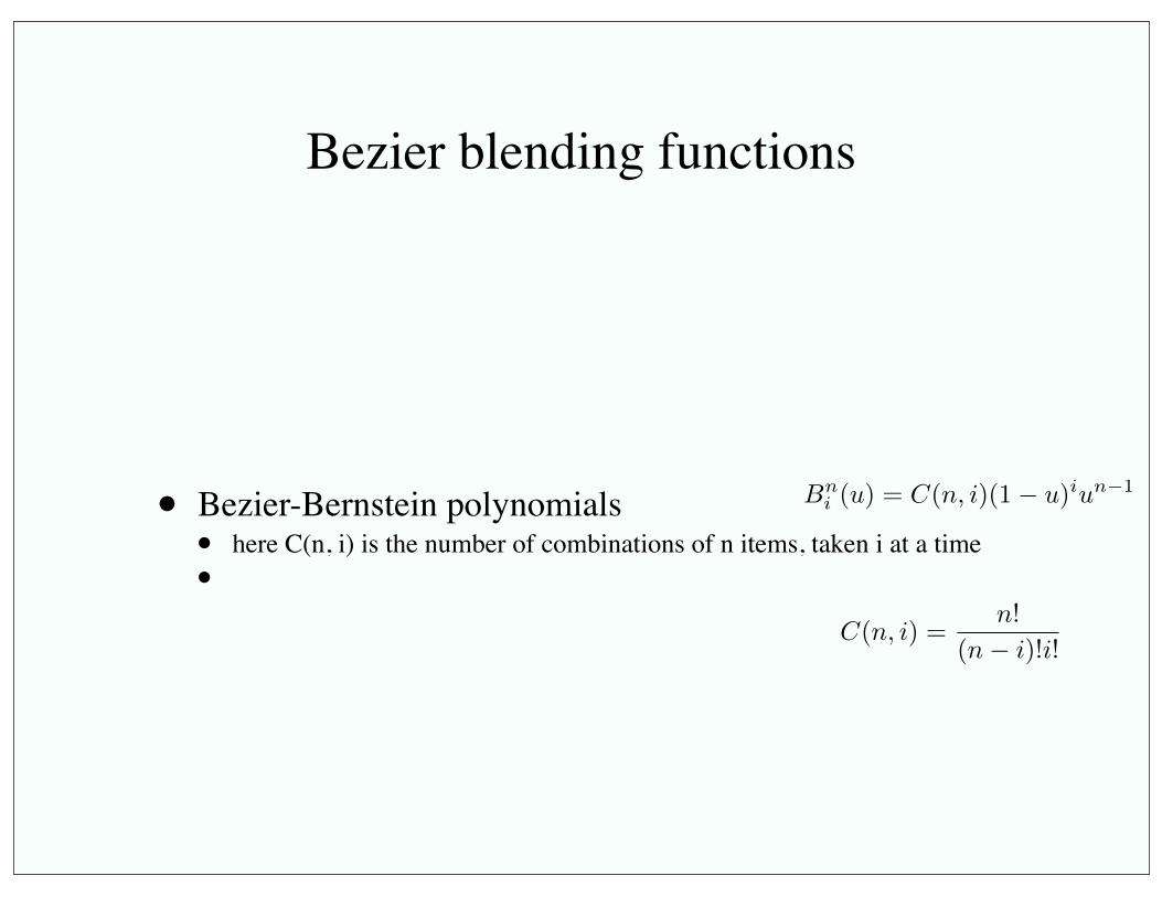
Bezier blending functions

• Bezier-Bernstein polynomials• here C(n, i) is the number of combinations of n items, taken i at a time•

Bni (u) = C(n, i)(1� u)iun�1

C(n, i) =n!

(n� i)!i!

Bezier curve properties

• Pass through first, last points• Tangent to initial, final segments of control polygon• Lie within convex hull of control polygon• Subdivide

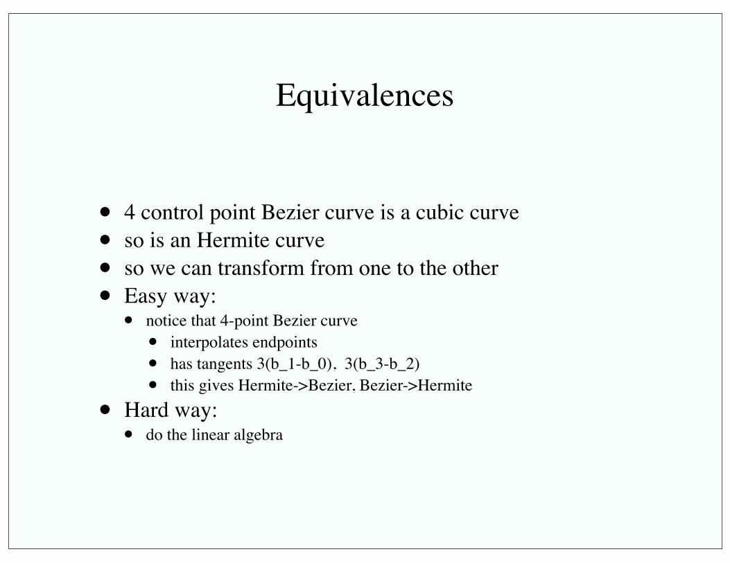
Equivalences

• 4 control point Bezier curve is a cubic curve• so is an Hermite curve• so we can transform from one to the other• Easy way:

• notice that 4-point Bezier curve• interpolates endpoints• has tangents 3(b_1-b_0), 3(b_3-b_2)• this gives Hermite->Bezier, Bezier->Hermite

• Hard way:• do the linear algebra

4-point Bezier curve:

Hermite curve:

⇥1 t t2 t3

⇤

8>><

>>:

1 0 0 0�3 3 0 03 �6 3 0�1 3 �3 1

9>>=

>>;

2

664

p0

p1

p2

p3

3

775

⇥1 t t2 t3

⇤

8>><

>>:

1 0 0 00 0 1 0�3 3 �2 �12 �2 1 1

9>>=

>>;

2

664

p0

p1

v0

v1

3

775

⇥1 t t2 t3

⇤BbGb

⇥1 t t2 t3

⇤BhGh

• Say we know G_b • what G_h will give the same curve?

• known G_h works similarly

Converting

BhGh = BbGb

Gh = B�1h BbGb

Joining up curves

• Two kinds of join• Geometric continuity

• G^0 - end points join up• G^1 - end points join up, tangents are parallel• Idea: the curves *could* be parametrized with a C^0 (C^1)

parametrization, but currently are not• Very important in modelling

• Parametric continuity, or continuity• C^0 - the parameter functions of the curve are continuous• C^1 - the parameter functions are continuous, have continuous deriv• C^2 - .. .. .. .. and continuous second deriv• Very important in animation (the parametrization is usually time)

Simple cases

• Join up two point Hermite curves• endpoints the same, vectors not - G^0• endpoints, vectors the same - G^1 (easy)• endpoints the same, vectors same direction - G^1 (harder)• Catmull Rom construction if we don’t know tangents

• Subdivide a Bezier curve• result is G^infinity if we reparametrize each segment as we should

• but not necessarily if we move the control points!

• Join up Bezier curves• endpoints join - G^0• endpoints join, end segments collinear - G^1

Catmull-Rom construction (partial)

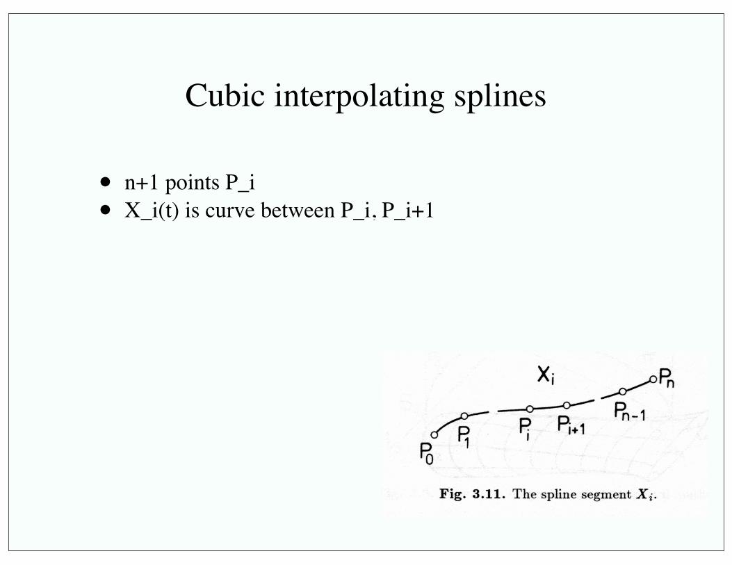
Cubic interpolating splines

• n+1 points P_i• X_i(t) is curve between P_i, P_i+1

Interpolating Cubic splines, G^1

• join a series of Hermite curves with equal derivatives.• But where are the derivative values to come from?

• Measurements

• Cardinal splines• average points• t is “tension”• specify endpoint tangents

• or use difference between first two, last two points

dXi

dt(0) =

1

2(1� t)(Pi+1 �Pi�1)

Tension

Interpolating Cubic splines: C^2

• One parametrization for the whole curve• divided up into intervals, called knots

• In each segment, there is a cubic curve FOR THAT SEGMENT

• And we must make this lot C^2

ti t < ti+1

Ai(t� ti)3 +Bi(t� ti)

2 +Ci(t� ti) +Di

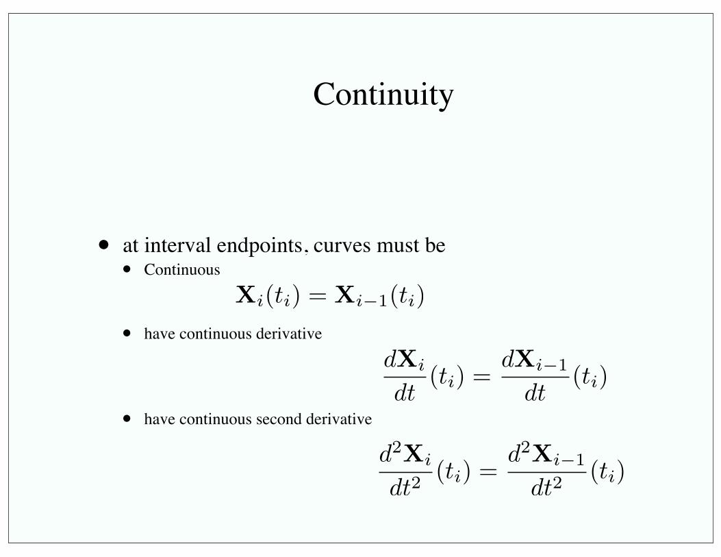
• at interval endpoints, curves must be• Continuous

• have continuous derivative

• have continuous second derivative

Continuity

Xi(ti) = Xi�1(ti)

d2Xi

dt2(ti) =

d2Xi�1

dt2(ti)

dXi

dt(ti) =

dXi�1

dt(ti)

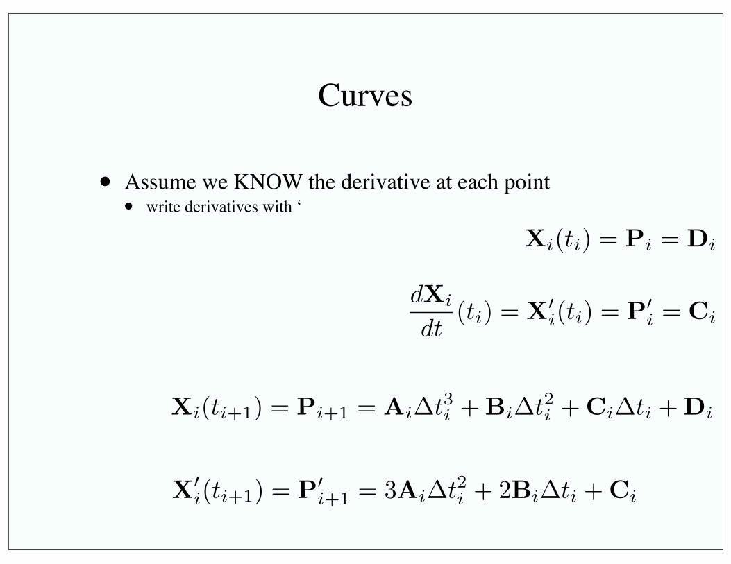
Curves

• Assume we KNOW the derivative at each point• write derivatives with ‘

Xi(ti) = Pi = Di

dXi

dt(ti) = X0

i(ti) = P0i = Ci

Xi(ti+1) = Pi+1 = Ai�t3i +Bi�t2i +Ci�ti +Di

X0i(ti+1) = P0

i+1 = 3Ai�t2i + 2Bi�ti +Ci

Curves

Xi(t) = Pi

✓2(t� ti)3

(�ti)3� 3

(t� ti)2

(�ti)2+ 1

◆+

Pi+1

✓�2

(t� ti)3

(�ti)3+ 3

(t� ti)2

(�ti)2

◆+

P0i

✓(t� ti)3

(�ti)2� 2

(t� ti)2

(�ti)+ (t� ti)

◆+

P0i+1

✓(t� ti)3

(�ti)2� (t� ti)2

(�ti)

◆

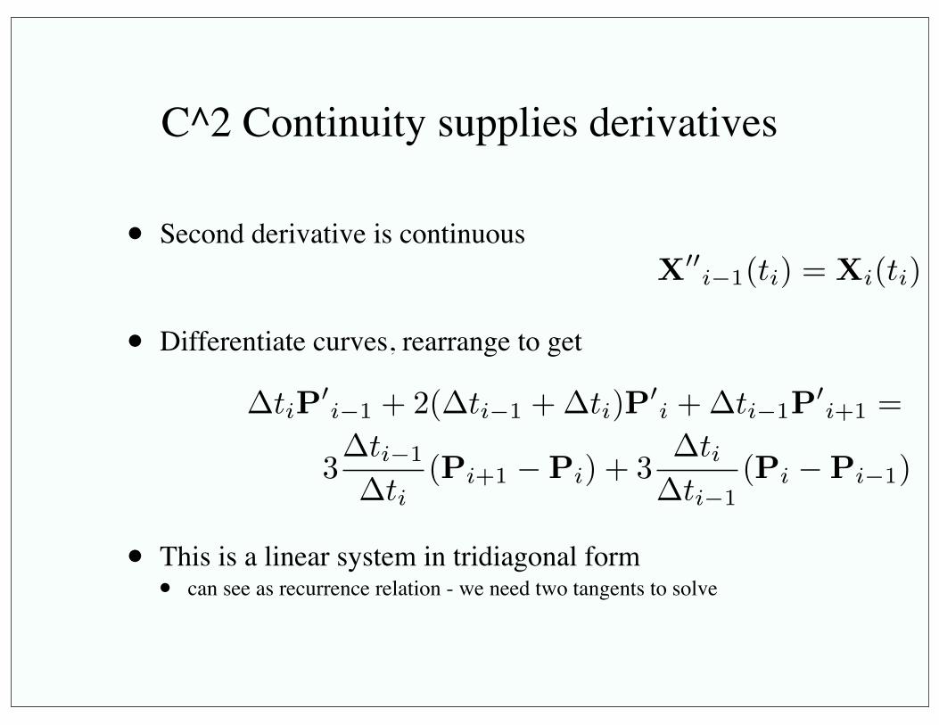
C^2 Continuity supplies derivatives

• Second derivative is continuous

• Differentiate curves, rearrange to get

• This is a linear system in tridiagonal form• can see as recurrence relation - we need two tangents to solve

X00i�1(ti) = Xi(ti)

�tiP0i�1 + 2(�ti�1 +�ti)P

0i +�ti�1P

0i+1 =

3�ti�1

�ti(Pi+1 �Pi) + 3

�ti�ti�1

(Pi �Pi�1)

C^2 cubic splines

• Recurrence relations • d(n-1) equations in d(n+1) unknowns (d is dimension)

• Options:• give P’_0, P’_1 (easiest, unnatural)• second derivatives vanish at each end (natural spline)• give slopes at the boundary

• vector from first to second, second last to last• parabola through first three, last three points• third derivative is the same at first, last knot

More general splines

• We would like to retain continuity, local control• but drop interpolation

• Mechanism• get clever with blending functions• continuity of curve=continuity of blending functions• we will need to “switch” on or off pieces of function

• e.g. linear example

• This takes us to B-splines, which you know• so we’ll move on to surface constructions