internet topologies and their modelling
TRANSCRIPT

1
83962 Design Project in Telecommunications
Harri Marjamäki, 127046
Internet topologies and their modelling

2

i
TABLE OF CONTENTS
TABLE OF CONTENTS I
ABSTRACT III
TIIVISTELMÄ III
TABLE OF FIGURES V
LIST OF TABLES V
LIST OF ABBREVIATIONS V
1. INTRODUCTION 1
2. THE HISTORY OF THE INTERNET 3
2.1. To ARPANET 3
2.2. ARPANET to NSFNET 4
2.3. NSFNET to Internet 5
3. NETWORKS IN PRACTICE 7
3.1. Topological aspect 7
3.2. Metric aspect 8
3.3. Example networks 8
4. GRAPH GENERATION METHODS 11
4.1. Flat random methods 11
4.2. Regular topologies 13
4.3. Hierarchical methods 15
4.3.1. N-level method 15
4.3.2. Transit-Stub method 16
5. GRAPH METRICS 19
5.1. Topological metrics 19
5.2. Example application metrics 20
5.3. Metrics of actual networks 21
6. GRAPH GENERATION SOFTWARE 23
6.1. Tiers 23
6.1.1. Tiers network model 23
6.1.2. Tiers network model parameters 24
6.1.3. Tiers sample graphs 25
6.2. GT-ITM 29
6.2.1. GT-ITM network models 29

ii
6.2.2. GT-ITM network model parameters 29
6.2.3. GT-ITM sample graphs 31
6.3. RTG 31
6.3.1. RTG network models 31
6.3.2. RTG network model parameters 31
6.3.3. RTG sample graphs 31
6.4. Comparison of implementations 33
7. CONCLUSIONS 35
REFERENCES 37
APPENDIX 1: A GT-ITM graph file 39
APPENDIX 2: A GT-ITM evaluation results file 45

iii
ABSTRACT
The purpose of this project work is to review the basic topological structure of the
Internet and present different modelling methods that have been developed to produce
graphs that can be used for example for testing and development of routing algorithms. In
the experimental part of this project some topology generating softwares will be installed
and tested and some sample topologies will be generated.
TIIVISTELMÄ
Tämän projektityön tarkoitus on kuvata Internetin topologista rakennetta sekä esitellä
erilaisia mallinnusmenetelmiä, joita käytetään topologioiden generointiin. Generoituja
topologioita voidaan hyödyntää esimerkiksi reititysalgoritmien testaamisessa ja
suunnittelussa. Työn kokeellisessa osassa asennetaan ja testataan joitakin topologioiden
generointiin kehitettyjä ohjelmia, sekä tuotetaan esimerkkitopologioita.

iv

v
TABLE OF FIGURES
Figure 2-1: ARPANET in September 1971 4Figure 2-2: Growth of the Internet 5Figure 2-3: World connectivity map 6Figure 3-1: CERFnet backbone topology 9Figure 3-2: UVA Network Topology 9Figure 3-3: Network Topology of Northwestern Polytechnic University 10Figure 4-1: Bus topology 14Figure 4-2: Ring topology 14Figure 4-3: Star topology 14Figure 4-4: Mesh topology 14Figure 4-5: N-level hierarchical layout 16Figure 4-6: Transit-Stub model 17Figure 6-1: Tiers graph 1: WAN 26Figure 6-2: Tiers graph 1: WAN+MAN 26Figure 6-3: Tiers graph 1: WAN+MAN+LAN 27Figure 6-4: Tiers graph 2: WAN 27Figure 6-5: Tiers graph 2: WAN+MAN 28Figure 6-6: Tiers graph 2: WAN+MAN+LAN 28Figure 6-7: An RTG graph with 10 nodes 32Figure 6-8: An RTG graph with 100 nodes 32
LIST OF TABLES
Table 4-1: Flat random graph methods 13Table 5-1: Properties of regular graphs 20Table 5-2: Properties of real internetwork topologies 21Table 6-1: Used network model parameters for tiers 25
LIST OF ABBREVIATIONS
AAL ATM Adaptation LayerARPANET Advanced Research Project Agency NetworkATM Asynchronous Transfer ModeBITNET A network that was set up to allow for the transfer of E-mailCREN Computer Research Engineering NetworkCSNET Computer Science NetworkDoD Department of DefenceFDDI Fiber Distributed Data InterfaceIP Internet ProtocolISP Internet Service ProviderLAN Local Area NetworkMAN Metropolitan Area NetworkMILNET Military Network.NSF National Science FoundationSAP Service Access PointT1 A dedicated line that can carry 1.5 Mb/sTCP/IP Transmission Control ProtocolWAN Wide Area Network

vi

1
1. INTRODUCTION
The explosive growth of networking, and particularly of the Internet, has been
accompanied by a wide range of internetworking problems related to routing, resource
reservation, and administration. The study of algorithms and policies to address such
problems often involves simulation or analysis using an abstraction or model of the actual
network structure. The reason for this is clear: networks that are large enough to be
interesting are also expensive and difficult to control, therefore they are rarely available
for experimental purposes. Moreover, it is generally more efficient to assess solutions
using analysis or simulation, provided the model is a “good” abstraction of the real
network.
Historically, large networks such as the Public Switched Telephone Network have grown
according to a topological design developed by some central authority or administration.
In contrast, there is no central administration that controls, or even keeps track of, the
detailed topology of the Internet. Although its general shape may be influenced to some
small degree by policies for assignment of IP addresses and government funding of
interdomain exchange points, the Internet, for the most part, just grows. The technology
used to route and forward packets is explicitly designed to operate in such an
environment. Today’s Internet can be viewed as a collection of interconnected routing
domains. Each routing domain is a group of nodes (routers, switches and hosts) under a
single (technical) administration that share routing information and policy.
The topological structure of a network is typically modelled using a graph, with nodes
representing switches or routers, and edges representing direct connections (transmission
links or networks) between switches or routers. Thus, the graph models paths, sequences
of nodes, along which information flows between nodes in an internetwork. For example,
a FDDI ring to which four IP routers are connected would be represented as a completely
connected graph of four nodes. Hosts can also be represented as nodes; the typical host
will be represented as a leaf connected to a single router node.
Additional information about the network can be added to the topological structure by
associating information with the nodes and edges. For example, nodes might be assigned
numbers representing buffer capacity. An edge might have values of various types,
including costs, such as the propagation delay on the link, and constraints, such as the
bandwidth capacity of the link.

2
The purpose of this project work is to review the basic topological structure of the
Internet, including a brief history of the Internet and its development. Then we will
present modelling methods designed to produce graphs and also the metrics used to
evaluate them. Finally, three different software tools for generating graphs will be
presented and compared. The differences between the implementations may be of
importance in choosing an implementation for use.

3
2. THE HISTORY OF THE INTERNET
By definition the word internet means a collection of networks that are joined together.
Thus, the word Internet, with a capital 'I', means 'The collection of networks that are
joined together.' But what is the Internet, really, and how did it evolve ?
2.1 To ARPANET
The history of the Internet begins with the RAND group in 1966. Paul Baran was
commissioned by the U.S. Air Force to do a study on how it could maintain its command
and control over its missiles and bombers, after a nuclear attack. Baran's finished
document described several ways to accomplish this task. What he finally proposes is a
packet switched network. This network would have no central hub, and no central control
center. Instead it would have lines linking various places together.
Packets would be forwarded from place to place until they arrived at the proper
destination. The theory was that if the middle of the country were taken out by a nuclear
attack, the coasts could still talk to one another. This would be done by routing traffic
around the missing links through Canada, satellites, or possibly by going around the
world. In 1969 what would later become the Internet was founded. It contrasts sharply
with today's Internet. The ARPANET network had four machines on it, linked together
with a packet switched network.
In 1973 Cerf and his group developed the protocols that were to be called TCP/IP,
Transmission Control Protocol/ Internet Protocol. In 1976 the U.S. DoD began to
experiment with this new protocol and soon decided to require it for use on ARPANET.
January 1983 was the date fixed as when every machine connected to ARPANET had to
use this new protocol. Also, at this time is when ARPANET ceased to be and the
INTERNET came into being, for practical purposes. ARPANET was not officially taken
out of service until 1990. What this means is that the actual 56Kbs lines were taken out of
service. But, because the network is designed to route around missing parts no one
noticed that they were gone. Those people that were still using the lines received some
sort of a new connection to the NSF backbone. As a side note in 1984 the DoD decided to
form MILNET out of the ARPANET. This was done to ensure that the military would
have a reliable network to use for communication, while the ARPANET could still be
used for advanced wide area network testing [1].

4
Figure 2-1: ARPANET in September 1971 [2]
2.2. ARPANET to NSFNET
In 1984 the National Science Foundation got into the act of networking. The NSF felt that
it would be good to setup super computer centers that people could purchase time on for
research. Five centers for super computer research were established and each was linked
via a backbone to the others. This NSF backbone was also linked to ARPANET. The
NSF backbone has been upgraded rather frequently over the years and the amount of
traffic that it was capable of carrying and did carry soon over took ARPANET.
In 1984 NSF realized that the infrastructure of the network needed to be upgraded. They
also realized that they did not want to be in the network administration business. Merit,
MCI, IBM and the state of Michigan won a proposal to upgrade and manage the new
network, this agreement was for a five year time period with an option for renewal. MCI
would provide the T1 lines,1.5 Mbps which is twenty-five times faster than the old 56
Kbps lines, IBM would provide advanced routers and Merit would manage the network.
In 1985 the National Science Foundation began deploying its new T1 lines. By 1988 this
new network was up and running and it had been done on time and within budget.
Merit and its partners formed a not for profit corporation called ANS, Advanced Network
Systems, which was to conduct research into high speed networking. It soon came up
with the concept of the T3, a 45 Mbps line. NSF quickly adopted the new network and by

5
the end of 1991 all of its sites were connected by this new backbone. During the time that
it took to make this transition, three years, the network had grown incredibly. There were
now 4,500 different networks connected to the NSF backbone, as opposed to 170 in 1986.
In Figure 2-2 below you can see how the Internet grew on a monthly basis after its
creation. The graph clearly shows that the growth of the Internet has been rapid since the
beginning of 1990s. Also the number of packets travelling the network had increased to
12.2 billion, during a month, from 162 million in 1986. These growth rates were
incredible and made the National Science Foundation wonder what the future held for the
Internet [1].
Figure 2-2: Growth of the Internet
2.3. NSFNET to Internet
In 1987 CREN was formed out of a merger of BITNET and CSNET. CREN maintained
those existing services and provided access to the Internet. But, CREN started to do
research and would later develope the World Wide Web.
The years 1991 to 1994 were years of growth and stability for the Internet. No major
changes were made to the physical network. The most significant thing that happened
was the growth. Many new networks were added to the NSF backbone. Hundreds of
thousands of new hosts were added to the Internet during this time period. Also,

6
significant new uses of the net were found. CREN developed the technology for the
World Wide Web, which quickly became the second most used application on the
Internet, based on the amount of data transferred.
It is estimated that today almost every country in the world is connected to the Internet in
one form or another. Below in Figure 2-3 is a map of the world showing how different
countries were connected in June of 1997 [3]. The number of hosts in the Internet was
36.7 million in July of 1998 [16].
Figure 2-3: World connectivity map

7
3. NETWORKS IN PRACTICE
A network has topological and metric aspects, that is, how the network is connected and
what makes up the connections [4].
3.1. Topological aspect
Considering the topological aspect first, a network can be represented by a graph at any
layer, from the physical layer to the application layer. The graph for each layer may be
different. For instance, two nodes which are physically connected may be unconnected at
the network layer if they reside on different network layer subnets. Generally, graphs
used for testing routing algorithms are a combination of the graphs for the network and
all lower layers. The graph is supposed to represent all possible sources and destinations
for data, usually assuming an endpoint is a source and/or destination at each node in the
graph.
For example, a multi-homed IP connected host with two IP addresses, would be
represented as two nodes in the network layer graph of a network. When considering
ATM connections, an endnode would represent an AAL Service Access Point (SAP),
since it cannot be assumed that replication can be done during reassembly in the AAL.
An intermediate node in an ATM network may represent only the lower sublayer of the
AAL, where a cell is replicated and switched to its destinations. If the switch contains one
of the destinations, then that node also represents an AAL SAP.
The edges of a network graph represent the possible paths which may be taken from a
source to a destination. In a simple network, there is only one path from source to
destination. Extra paths come from redundancy being introduced at the network layer or
lower layers. Such redundancy could be in the form of a second physical connection
between hosts in a LAN, a second connection to a bridge to other LANs, or a second
router attached to a LAN. In the wide area, nodes are often physically separated by wide
distance but interconnected in a relatively dense manner to avoid ‘back-hoe loss’ and
have multiple paths at the other layers too. Since such redundancy incurs extra equipment
and configuration costs, it is more likely to occur in the critical areas of a network, such
as closer to a backbone, and also in networks used in failure sensitive situations or for
real-time control [4].

8
3.2. Metric aspect
Now consider the metric aspect of modelling networks. The two types of metrics which
occur in networks are constraints and metrics which are to be minimized (or maximized).
An example of a constraint is the bandwidth on a link. An example of a metric to be
minimized is the transmission delay between a source and a destination. For the purposes
of modelling, the transmission delay is often taken to be proportional to the physical
distance between two points, with the addition of fixed processing overhead at certain
nodes (e.g. routing from one subnet to another). Bandwidth is generally taken to be fixed
and assumed to be shared in a linear fashion, i.e. one connection of 10 Mb/s is equivalent
to ten connections of 1 Mb/s each. As a passing observation, this last assumption
probably only holds true for large numbers of connections or routes on a link [4].
3.3. Example networks
As an example, Figures 3-1 to 3-3 present some actual network topologies. Figure 3-1
presents a nationwide backbone topology, Fig. 3-2 presents the router level topology of
The University of Virginia and Fig. 3-3 presents the router and LAN level topology of
Northwestern Polytechnic University. A series of observations can be drawn from
considering the theoretical action of the network layer.
- As expected, redundancy, in terms of multiple paths between nodes, increases the
more ‘central’ a node is in the network.
- Most nodes have very few paths to other nodes.
- Almost no nodes at the ‘edge’ of the network have connections directly to other edge
nodes outside their own geographic area.
- Shared media topologies are common in the LAN, either as a bus, ring or star.
As many as possible of these properties should be modelled in a good graph generation
method. Different graph generation methods are discussed in the next chapter.

9
Figure 3-1: CERFnet backbone topology [17]
Figure 3-2: UVA Network Topology [5]

10
Figure 3-3: Network Topology of Northwestern Polytechnic University [6]

11
4. GRAPH GENERATION METHODS
When modelling an entity with some details that are unknown, or may vary, the standard
approach is to substitute nondeterminism for the unknowns, generate multiple instances,
and analyze the set of results. In modelling Internet topology, this corresponds to
generating multiple graphs to be used in simulation or analytic studies. In this section, we
consider three classes of generation methods.
The first are flat random graph methods, which construct a graph by probabilistically
adding edges to a given set of nodes, with no structure amongst the nodes. The second
class of generation methods are regular, in the sense that they generate graphs with
specific structure, for example rings and meshes, and thus have no randomness at all. The
third class of models are hierachical, building larger network structure from smaller
network components. These methods represent a compromise between the extremes of
the flat random and regular methods: they impose some high level structure, and fill in
details at random [7].
4.1. Flat random methods
The networking literature contains a variety of flat (i.e., non-hierarchical) random
methods used to model internetworks. All are variations on the standard random graph
model that distributes vertices at random locations on a plane and then considers each
pair of vertices; an edge is added between a pair of vertices with probability α. We call
this the Pure Random model or simply the Random model. While it does not explicitly
attempt to reflect the structure of real internetworks, it is attractive for its simplicity and
is commonly used to study networking problems.
The other models also distribute the vertices randomly in the plane, however they alter
the function used for the probability of an edge, in an attempt to better reflect real
network structure. After the Pure Random Model, perhaps the most common random
graph model is the one proposed by Waxman [8], with the probability of an edge from u
to v given by:
)/(*),( LdevuP βα −= (4.1)
where 0 < α, β ≤ 1, d is the Euclidean distance from u to v and scaleL *2= is the
maximum distance between any two nodes. An increase in α will increase the number of

12
edges in the graph, while an increase in β will increase the ratio of long edges relative to
shorter edges. We call this the Waxman 1 model.
Several variations on the Waxman model have been proposed. They include:
- Replacing d by a random number between 0 and L [8]. We call this the Waxman 2
model.
- Scaling P(u,v) by a factor kε/n, where ε is the desired average node degree, n is the
number of nodes and k is a constant that depends on α and β [9]. This is called the
Doar-Leslie model.
- Allowing α > 1.0 [10].
The second model, while not fundamentally different than the Waxman model, is
interesting because the addition of the factor radius = kε gives more direct control over
the number of edges in the graphs that are generated, provided k is known. Clearly the α
parameter of the Waxman model can be chosen to be equivalent to any particular setting
of the parameters k, ε, n and α in the Doar-Leslie model.
In [11], an exponential method is presented. This method uses:
)/(*),( dLdevuP −−= α (4.2)
so that the probability of an edge approaches zero as the distance between two vertices
approaches L.
The locality method, also presented in [11], partitions the (potential) edges based on
length, and assigns a different (fixed) probability for each equivalence class of edge
lengths. For the case of two equivalence classes, the parameter radius defines the
boundary:
≥<
=radiusLd
radiusLdvuP
*,
*,),(
βα
(4.3)
To summarize, Table 4-1 indicates the probability of an edge between two vertices at
Euclidean distance d for each flat random method in our study.

13
Table 4-1: Flat random graph methods
Method Edge probability
Pure random α
Waxman 1 )/(* Lde βα −
Waxman 2 )/(),0(* LLrande βα −
Doar-Leslie )/()/( Ldenk βεα −
Exponential )/(* dLde −−α
Locality
≥<
radiusLd
radiusLd
*,
*,
βα
Note that in each of these methods, every pair of vertices is treated equally with respect to
addition of edges. Thus, although it is possible to control the approximate number of
edges, it is not possible to control the configuration of the edges. This has implications
for the generation of large sparsely-connected graphs using these methods. In particular,
for any of the edge probability functions in Table 4-1, the probability that a graph is
connected decreases as number of nodes in the graph increases. As a result, it is difficult
to create connected graphs with large numbers of nodes and low average node degree.
One alternative is to generate partially-connected graphs and then apply various “repair”
techniques to connect the graph. Obviously this will produce graphs whose structure is
not entirely random, because it has been influenced by the repair process. Another option
is to use the random methods to generate smaller graphs that are then connected into a
hierarchical structure.
4.2. Regular topologies
Regular topologies are often used in analytic studies of algorithmic performance because
their structure makes them tractable. We consider buses, rings, stars and meshes. Figures
4-1 to 4-4 give an example of each topology. The general structure should be clear from
these examples.

14
Figure 4-1: Bus topology
Figure 4-2: Ring topology
Figure 4-3: Star topology
Figure 4-4: Mesh topology

15
4.3. Hierarchical methods
The flat random and regular graph methods represent extremes in the sense that the
former offer little control over the structure of the resulting graphs, while the latter are
extremely rigid in their structure. Neither captures the hierarchy that is present in real
internetworks, though both may reflect some notion of locality if certain nodes are more
likely to be connected than others. We now describe two methods of creating hierarchical
graphs by connecting smaller components together according to a larger-scale structure
[7].
4.3.1. N-level method
The N-level hierarchical method constructs a graph by iteratively expanding individual
nodes into graphs. Beginning with a connected graph, each node in the graph is replaced
by a connected graph. The edges of the original graph are then re-attached to nodes in the
replacement graphs.
More precisely, in constructing the flat random graphs, we divide a unit square in the
Euclidean plane into equal-sized square sectors, the number of which is determined by a
scale parameter S; each node in the graph is then assigned to one of the 2S squares. In
constructing an N-level hierarchical graph, the top-level graph is constructed in this
fashion using scale parameter 1S . Then each square containing a node is subdivided
again, according to the second-level scale parameter 2S , and a graph is constructed using
that top-level square as the unit plane.
Figure 4-5 illustrates the initial iterations of the process. The result is that the scale of the
final graph is the product of the scales of the individual levels, and edge lengths are
roughly determined by edge level. For example, in a three-level graph, top-level edges
(i.e., part of the original graph) are typically longer than second-level edges, while the
second-level edges are typically longer than third-level edges [7].

16
Figure 4-5: N-level hierarchical layout
4.3.2. Transit-Stub method
Transit-Stub method is presented in [12]. In this model each routing domain in the
Internet can be classified as either a stub domain or a transit domain. A stub domain
carries only traffic that originates or terminates in the domain. Transit domains do not
have this restriction. The purpose of transit domains is to interconnect stub domains
efficiently, without them, every pair of stub domains would need to be directly connected
to each other (see figure 4-6). Stub domains generally correspond to campus networks or
other collections of interconnected LANs, while transit domains are almost always wide-
or metropolitan-area networks (WANs or MANs).
A transit domain consists of a set of backbone nodes. In a transit domain each backbone
node may also connect to a number of stub domains, via gateway nodes in the stubs.
Some backbone nodes also connect to other transit domains. Stub domains can be further
classified as single- or multi-homed. Multi-homed stub domains have connections to
more than one transit domain, single-homed stubs connect to only one transit domain.
Some stub domains may have links to other stubs. Transit domains may themselves be
organized in hierarchies, e.g. MANs connect mainly to stub domains and WANs.

17
Figure 4-6: Transit-Stub model

18

19
5. GRAPH METRICS
In this section, we consider several metrics that can be used to compare and evaluate
graphs. The metrics fall into two categories: topological metrics, which are independent
of any particular application, and application-specific metrics, which depend on topology
and application [7].
5.1. Topological metrics
We first consider attributes inherent in the graphs themselves; these are useful for
characterizing and classifying methods independent of any particular application. Some
of these metrics are derived from shortest paths; we consider both “hop” metrics, in
which each edge has unit weight, and “length” metrics, in which each edge has weight
equal to its Euclidean length. We further consider composite metrics in which the shortest
paths are determined using one metric, but evaluated using a different metric.
For example, in the hierarchical methods, we might determine the shortest paths using the
routing policy weights, then evaluate the maximum hop count for these (policy-
determined) routes between nodes.
For a graph with n nodes and m edges, we consider the following topological properties:
- Average node degree. (2m/n)
- Diameter. The diameter of a graph is the length of the longest shortest-path between
any two vertices. Informally, a low diameter generally corresponds to shorter paths.
We consider several variations on the diameter, depending on the metric used to
construct and evaluate the shortest paths.
- The hop-diameter is the length of the longest shortest-path between any two vertices,
where the shortest paths are computed and evaluated using hop count as the metric.
- The length-diameter is the length of the longest shortest-path between any two
vertices, where the shortest paths are computed and evaluated using Euclidean length
as the metric.
- The hop-length-diameter is a composite metric. The shortest paths are determined
using hop count, then measured using Euclidean length. The diameter is the longest
Euclidean length amongst the paths found using hop count. This metric is interesting
because routing algorithms often use hop count to find paths, but propagation delay is
proportional to physical path length (represented by Euclidean distances).

20
- For the hierarchical methods, the policy-hop-diameter uses the routing policy
weights to construct the shortest paths, then uses the hop count to evaluate the length
of the paths. The diameter is the length of the longest path.
- Similarly, the policy-length-diameter uses the routing policy weights to construct the
shortest paths, then uses the Euclidean length to evaluate the length of the paths. The
diameter is the length of the longest path.
- Number of biconnected components. A biconnected component (or bicomponent) is
a maximal set of edges such that any two edges in the set are on a common simple
cycle. The number of bicomponents is a measure of the degree of “connectedness” or
”edge redundancy” in a graph. Generally, a larger number of bicomponents
corresponds to a larger number of paths between nodes in the graph.
As an example, Table 5-1 gives selected properties of buses, rings, stars and meshes, with
n nodes. While a ring and a bus differ by only one edge, they have substantially different
hop-diameter and number of bicomponents. (Removing one edge in a ring breaks the
symmetry.) A star has the smallest hop-diameter of these four regular graphs. In all cases,
the properties are completely determined by the number of nodes n.
Table 5-1: Properties of regular graphs
Edges Hop-diameter Bicomps
Bus n-1 n-1 0
Ring n n/2 n
Star n-1 2 0
Mesh )(2 nn − )1(2 −n )(2 nn −
5.2. Example application metrics
To more closely relate the evaluation of network models to a specific intended use, we
also consider two metrics that are relevant to the performance of multicast routing
algorithms. Briefly, a multicast routing instance is a subset S of the graph nodes
designated as multicast group sources and another subset R designated as multicast group
receivers; these two sets may intersect.
For a given graph and instance, a multicast routing algorithm defines a set of distribution
trees, one per source, which determine the path followed by each packet sent by a source
on its way to all the receivers. A distribution tree is generally derived from the shortest-

21
path trees provided by the underlying internetwork (unicast) routing protocol. For a group
with s senders and r receivers (1 ≤ s, r ≤ n) we measure the following quantities for
multicast routing algorithm A:
- Packet-hops ratio. This metric considers the packet-hops, that is, the number of
edges traversed by multicast packets in the routing trees defined by A, from all
sources to all destinations. The actual value of the metric is the ratio of this quantity
to the packet-hops used by another routing algorithm that constructs a distribution
tree by using a shortest-path tree rooted at each source and including all receivers as
leaves.
- Delay ratio. This metric considers the maximum delay, measured in hops, from any
source to any receiver in the distribution trees defined by A. As above, the “raw”
value is normalized to get the metric value, by dividing by the maximum delay
obtained using a shortest-path algorithm. Note that this ratio is always at least 1.0.
5.3. Metrics of actual networks
Unfortunately, it is difficult to obtain complete topological descriptions of even a modest
portion of the Internet, due to the lack of any centralized administration. In fact, some
administrations go to great lengths to hide the topology of their network from the outside
world, for reasons of security. Metrics of some known topologies are presented in [11].
Table 5-2 shows these results.
Table 5-2: Properties of real internetwork topologies
Network Nodes Avg. Deg. Diam. Bicomp.
ARPAnet 47 2.9 9 5
CERFnet 63 2.1 5 59
Sesquinet 94 2.1 9 77
PGE 137 2.2 10 103
Ga. Tech 30 3.9 3 16
The ARPAnet entries refer to the “old ARPAnet” backbone, which has been used as a
topology in a number of simulation studies. CERFnet and Sesquinet are backbone
regional networks, i.e., they connect to (and carry traffic from) many smaller “stub”

22
networks. “PGE” is a large private network; the final entry reflects the characteristics of
Georgia Tech campus internet.
The statistics for ARPAnet reflect the backbone topology only, while those for CERFnet
and Sesquinet include edges to other routing domains. This gives the latter networks a
more tree-like structure, and thus a lower average node degree. PGE also has a substantial
number of “leaf” nodes, while the Georgia Tech network features a relatively high
degree of connectivity.

23
6. GRAPH GENERATION SOFTWARE
In this chapter we will present three different software utilities for generating graphs.
They are all available in public domain. We will present their network models and
parameters and show some sample graphs.
6.1. Tiers
Tiers is written by Matthew Doar and the source code for Tiers 1.2 is available at [13].
6.1.1. Tiers network model
The model has the following characteristics [4]:
- Shared media LANs such as Ethernet and Token Rings are modelled as star
topologies. This significantly reduces the number of edges in the graph and reflects
the lack of physical redundancy in most LANs. There may be hundreds of hosts in a
LAN. NBMA (Non-Broadcast Multiple Access) LANs such as switched Ethernet are
also modelled as stars, with the switch at the centre of the star.
- LANs should be modelled as being interconnected in small numbers, with some small
degree of redundancy in their connections.
- Each major institution has a small number of connections to a WAN service provider,
who is in turn connected to other Internet Service Providers (ISPs) in a highly
redundant fashion. Each ISP can be modelled as a single node and the WAN
modelled as a single layer for the purposes of simplification.
- To simplify the graph redundancy in the network is limited to redundancy seen at the
topmost (network) layer under consideration. Thus only routers in an IP network or
switches in an ATM network appear as non-edge nodes in the graph. Edge nodes are
the AAL SAPs in an ATM network and network layer SAPs in an IP network.
- The model shall be able to run using few floating point operations in order to decrease
simulation time when constructing thousands of network models with large number of
nodes.

24
Nodes are categorized into three broad categories: edge nodes (LAN nodes), bridge,
router or switch nodes (MAN nodes) and gateway (WAN nodes). When a host is part of a
LAN and a MAN (for instance) the host is represented as two interconnected nodes, a
LAN node and a MAN node. The metrics of the edge between the two types of nodes
reflect the processing delay and bandwidth constraints within the host.
The Tiers model produces connected subgraphs by joining all the nodes in a single
domain using a minimum spanning tree. The use of a minimum spanning tree is a crucial
feature of Tiers and is particularly appropriate since it is sometimes used in reality as the
basis for laying out large networks. When adding edges for intranetwork redundancy,
edges are added to the closest nodes in the network, in increasing order of Euclidean
distance. For internetwork redundancy, extra edges are added to the closest nodes in the
next higher domain. This ensures some degree of local connectivity within geographic
constraints [12].
6.1.2. Tiers network model parameters
A simple set of parameters is necessary to be able to repeatedly generate networks which
bear some resemblance to real networks. The major parameters for tiers model are [4]:
- WN , the number of WANs and WS , the number of nodes in a WAN. WN is taken as
1 for simplicity.
- MN , the number of corporate/institutional networks (MANs) and MS , the number of
nodes per MAN. Since every MAN is connected to at least one WAN node, WS ≥ 1.
- LN , the number of LANs per MAN and LS , the number of nodes per LAN. Again,
MS ≥ 1, since there is a MAN node for every LAN.
The total number of nodes in the graph, N, is given by:
LLMMMW SNNSNSN ++= (6.1)
Typical values might be: LS = 50, LN = 5 and MS = 10, MN = 10 and WN = 5 for a
corporate internet. This would make N equal to 2605 nodes. For a smaller graph,
modelling just the MAN and WAN environment, typical values might be LN = 0, MN =
10, MS = 5, and WN = 5 giving N = 55 nodes in the network.

25
The other parameters of the model are:
- The degree of intranetwork redundancy in the WAN (WR ), MAN ( MR ) and LAN
( LR ). This is expressed simply as the degree (number of directed edges) from a node
to another node of the same type. LR is usually 1, MR might be 2 and WR could be 3.
- The degree of internetwork redundancy between networks. This is the number of
connections between a MAN and a WAN (MWR ) or a LAN and a MAN ( LMR ).
A small table of costs and constraints associated with each type of edge is also defined as
part of the model. This table contains entries for the 3*3 = 9 kinds of edge: for a WAN to
MAN edge, a MAN to WAN edge, a LAN to MAN edge and so on. Each entry contains
constraints on the bandwidth and other characteristics such as the speed of transmission
in the media (often assumed constant in all parts of the network). For instance, to define
an ATM backbone in a company, the bandwidth constraint for MAN to MAN edges
might be set at 155 Mb/s. This table can also be used to describe characteristics such as
the processing delay in a router interconnecting two LANs, since this is where the LAN
to MAN edge characteristics are stored.
6.1.3. Tiers sample graphs
In this section we present some graphs that were generated using tiers. Tiers provides
output format for gnuplot 3.6 or higher which provides a visual representation of the
graph. Table 6-1 presents the used parameters for the graphs.
Table 6-1: Used network model parameters for tiers
WN MN LN WS MS LS WR MR LR MWR LMR
Graph 1 1 25 2 40 6 6 2 2 1 1 1
Graph 2 1 50 5 150 9 5 3 2 1 2 1

26
Figure 6-1: Tiers graph 1: WAN
Figure 6-2: Tiers graph 1: WAN+MAN

27
Figure 6-3: Tiers graph 1: WAN+MAN+LAN
Figure 6-4: Tiers graph 2: WAN

28
Figure 6-5: Tiers graph 2: WAN+MAN
Figure 6-6: Tiers graph 2: WAN+MAN+LAN

29
6.2. GT-ITM
GT-ITM (Georgia Tech Internetwork Topology Models) is written by Ellen Zegura. The
source codes for GT-ITM are available at [14].
6.2.1. GT-ITM network models
GT-ITM provides three different graph types: flat random, N-level hierarchy and Transit-
Stub. These methods were presented in chapter 4. GT-ITM provides also 6 different edge
models. These models were discussed in section 4.1.
The Transit-Stub model doesn’t support representation of host systems. Thus, all nodes
are of the same type, namely routers. The Transit-Stub model produces connected
subgraphs by repeatedly generating a graph according to the edge count and checking the
graph connectivity. Unconnected graphs are discarded. This method ensures that the
resulting subgraph is taken at random from all possible (connected) graphs; however, it
may take a long time to generate a connected graph if the edge count is relatively small.
Extra edges from stub domains to transit nodes are added by random selection of the
domains and nodes. The TS model also supports an additional parameter for indicating
the number of stub-to-stub edges. These edges are also added by random selection of the
domains and nodes involved [12].
6.2.2. GT-ITM network model parameters
The network model parameters for GT-ITM are:
- <method keyword> is one of:
“geo”: flat random graph
“hier”: N-level hierarchical graph
“ts”: transit-stub graph
- <number of graphs>: number of graphs of specified type to generate
- <initial seed>: initial random number seed; optional
- <method-dependent parameter lines>
All of the methods make use of the following <geo_parms> line, which specifies the
parameters for a flat random graph. Six different types (see Table 4-1) of flat random
graphs are supported.

30
<geo_parms> ::= <n> <scale> <edgemethod> <alpha> [<beta> <gamma> ]
<n>: number of nodes in graph
<scale>: one-sided dimension of space in which nodes are distributed
<edgemethod>: method for generating edges; valid range 1-6.
1: Waxman 1
2: Waxman 2
3: Pure random
4: Doar-Leslie
5: Exponential
6: Locality
<alpha>: random graph parameter (0 ≤ α ≤ 1)
<beta>: random graph parameter (0 ≤ β)
<gamma>: random graph parameter (0 ≤ γ)
The <method-dependent parameter lines> are as follows:
<”geo” parms> ::= <geo_parms>
<”hier” parms> ::= <number of levels> <edgeconnmethod> <threshold>
<geo_parms>+ {one per number of levels}
<number of levels>: number of levels in hierarchy
<edgeconnmethod>: method of resolving edges
0: random
1: use non-leaf node of smallest degree
2: use node of smallest degree
3: use first node with degree less than <threshold>
<threshold>: see above
<”ts” parms> ::= <#stubs/xit> <#t-s edges> <#s-s edges>
<geo_parms> {top-level parameters}
<geo_parms> {transit domain parameters}
<geo_parms> {stub domain parameters}
<#stubs/xit>: avg number of stub domains attached per transit node
<#t-s edges>: number of extra transit-stub edges
<#s-s edges>: number of extra stub-stub edges

31
Total number of parameters is 6-9 for flat random graph and 17-24 for 3-level and transit-
stub graph.
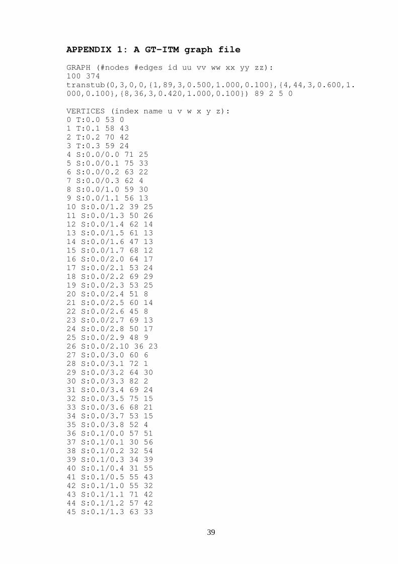
6.2.3. GT-ITM sample graphs
GT-ITM doesn’t provide a visual representation of graphs. Only textual output is
available. Output file of a transit-stub graph with 100 nodes is presented in Appendix 1.
This file contains nodes and their coordinates and edges with their lengths and weights.
GT-ITM software package includes a program for evaluating metrics of generated
graphs. A file representing evaluation results for the same graph is presented in Appendix
2.
6.3. RTG
RTG is written by Liming Wei and Lee Breslau. The source code for RTG is available at
[15].
6.3.1. RTG network models
RTG provides only flat random graphs in one level. Edges are connected using the
Waxman model.
6.3.2. RTG network model parameters
There are only two obligatory parameters in RTG. They are:
- Number of nodes
- Average node degree, from which α and β for Waxman’s equation are calculated.
Optional parameters are:
- Give direct value of α
- Give direct value of β
- Random seed for calculations
6.3.3. RTG sample graphs
RTG generates postscript output and has a built-in viewer. Figures 6-7 and 6-8 present
graphs with 10 and 100 nodes and average node degree 3.

32
Figure 6-7: An RTG graph with 10 nodes
Figure 6-8: An RTG graph with 100 nodes

33
6.4. Comparison of implementations
Tiers and GT-ITM provide hierarchical modelling approach whereas RTG only provides
one-level flat random modelled graphs. Tiers uses three-level hierarchical models while
GT-ITM has N-level and Transit-Stub models and also a flat random model is available.
Tiers provides a graphical output in Gnuplot format and RTG creates postscript output for
which it has a built-in viewer. GT-ITM provides only textual output format without any
visual representation of the graphs.
If we compare Tiers with GT-ITM, several differences can be found. Tiers introduces a
different method for connecting the nodes in a network, by using a minimum spanning
tree. The use of a minimum spanning tree guarantees connectivity, reduces the generation
time of the network, and produces more realistic networks at the WAN scale.
The GT-ITM implementation generates graphs using a more probabilistic approach than
that of Tiers, which in contrast uses a larger set of parameters to control the different
aspects of the networks produced.
A useful simplification introduced by Tiers to reduce number of edges, and hence
improve simulation times, is to model LAN topologies as stars. Another useful idea is to
treat a node that connects two types of networks as two nodes, with one node in each type
of network. This permits modelling of the delay in transferred data from one network to
another, which is often neglected in other network models.
Transit-Stub model of GT-ITM simplifies the network models by representing only
routers and switches. In addition, weights are associated with edges to produce paths that
follow standard Internet routing policy.

34

35
7. CONCLUSIONS
The issue of generating example networks is important for the testing of routing
algorithms and generating likely network deployment scenarios. This project work has
described the basic topological structure of the Internet, presented modelling methods
designed to produce graphs and also the metrics used to evaluate them. Also three
implementations were installed and tested and their main features and differences were
presented.
In the future, more data about the characteristics of the networks to be modeled has been
gathered, better distributions for the values of the model parameters can be defined.
Examining how the values of the parameters change with time may even help predict
how networks change within organizations.

36

37
REFERENCES
[1] http://clavin.music.uiuc.edu/sean/internet_history.html, October 1998.
[2] http://www.geog.ucl.ac.uk/casa/martin/atlas/historical.html, October 1998.
[3] ftp://ftp.cs.wisc.edu/connectivity_table/, October 1998.
[4] M. Doar, A Better Model for Generating Test Networks, IEEE Global
Telecommunications Conference/GLOBECOM'96, London, November 1996.
[5] http://www.itc.virginia.edu/~mjs/netinfo/maps/atm.gif, October 1998.
[6] http://www.npu.edu/network/network_Topology.html, October 1998.
[7] Ellen W. Zegura, Kenneth Calvert and M. Jeff Donahoo. A Quantitative Comparison
of Graph-based Models for Internet Topology. IEEE/ACM Transactions on Networking,
Volume 5, No. 6, December 1997.
[8] Bernard M. Waxman, Routing of multipoint connections. IEEE Journal on Selected
Areas in Communications, 6(9):1617-1622, 1988.
[9] Matthew Doar and Ian Leslie. How bad is naïve multicast routing?. Proceedings of
IEEE Infocom ’93, pp 82-89, 1993.
[10] Liming Wei and Deborah Estrin. The trade-offs of multicast trees and algorithms.
International Conference on Computer Communications and Networks, August 1994.
[11] Ellen W. Zegura, Ken Calvert and S. Bhattacharjee. How to Model an Internetwork.
Proceedings of IEEE Infocom '96, San Francisco, CA.
[12] Ken Calvert, Matt Doar and Ellen W. Zegura. Modeling Internet Topology. IEEE
Communications Magazine, June 1997.
[13] http://www.geocities.com/ResearchTriangle/3867/sourcecode.html, October 1998.
[14] http://www.cc.gatech.edu/fac/Ellen.Zegura/graphs.html, October 1998.
[15] http://www.cs.uoregon.edu/~zappala/src, October 1998.
[16] http://www.nw.com/zone/WWW/report.html, November 1998.
[17] http://www.cerf.net/cerfnet/about/Bbone-map/Bbone-large.gif, November 1998.

38
39
APPENDIX 1: A GT-ITM graph file
GRAPH (#nodes #edges id uu vv ww xx yy zz):100 374transtub(0,3,0,0,{1,89,3,0.500,1.000,0.100},{4,44,3,0.600,1.000,0.100},{8,36,3,0.420,1.000,0.100}) 89 2 5 0
VERTICES (index name u v w x y z):0 T:0.0 53 01 T:0.1 58 432 T:0.2 70 423 T:0.3 59 244 S:0.0/0.0 71 255 S:0.0/0.1 75 336 S:0.0/0.2 63 227 S:0.0/0.3 62 48 S:0.0/1.0 59 309 S:0.0/1.1 56 1310 S:0.0/1.2 39 2511 S:0.0/1.3 50 2612 S:0.0/1.4 62 1413 S:0.0/1.5 61 1314 S:0.0/1.6 47 1315 S:0.0/1.7 68 1216 S:0.0/2.0 64 1717 S:0.0/2.1 53 2418 S:0.0/2.2 69 2919 S:0.0/2.3 53 2520 S:0.0/2.4 51 821 S:0.0/2.5 60 1422 S:0.0/2.6 45 823 S:0.0/2.7 69 1324 S:0.0/2.8 50 1725 S:0.0/2.9 48 926 S:0.0/2.10 36 2327 S:0.0/3.0 60 628 S:0.0/3.1 72 129 S:0.0/3.2 64 3030 S:0.0/3.3 82 231 S:0.0/3.4 69 2432 S:0.0/3.5 75 1533 S:0.0/3.6 68 2134 S:0.0/3.7 53 1535 S:0.0/3.8 52 436 S:0.1/0.0 57 5137 S:0.1/0.1 30 5638 S:0.1/0.2 32 5439 S:0.1/0.3 34 3940 S:0.1/0.4 31 5541 S:0.1/0.5 55 4342 S:0.1/1.0 55 3243 S:0.1/1.1 71 4244 S:0.1/1.2 57 4245 S:0.1/1.3 63 33

40
46 S:0.1/1.4 41 5547 S:0.1/1.5 60 4448 S:0.1/1.6 58 4949 S:0.1/2.0 53 4950 S:0.1/2.1 79 3151 S:0.1/2.2 78 3452 S:0.1/2.3 60 2153 S:0.1/2.4 65 1654 S:0.1/2.5 59 2155 S:0.1/2.6 45 3356 S:0.1/2.7 55 3857 S:0.1/2.8 50 3958 S:0.1/2.9 71 1959 S:0.1/3.0 53 4560 S:0.1/3.1 49 6361 S:0.1/3.2 59 3962 S:0.1/3.3 68 3863 S:0.1/3.4 56 4564 S:0.1/3.5 58 3665 S:0.1/3.6 54 5766 S:0.1/3.7 37 5667 S:0.1/3.8 58 5368 S:0.2/0.0 73 4769 S:0.2/0.1 65 4870 S:0.2/0.2 75 5171 S:0.2/0.3 72 4772 S:0.2/0.4 54 2173 S:0.2/0.5 69 2874 S:0.2/0.6 80 4975 S:0.2/0.7 66 2676 S:0.2/0.8 55 4277 S:0.2/1.0 46 3378 S:0.2/1.1 64 3479 S:0.2/1.2 40 4180 S:0.2/1.3 63 5681 S:0.2/1.4 50 4082 S:0.2/1.5 56 5283 S:0.2/1.6 40 3184 S:0.2/1.7 68 2585 S:0.2/1.8 43 2886 S:0.2/1.9 59 2987 S:0.2/2.0 53 4488 S:0.2/2.1 47 4589 S:0.2/2.2 35 4290 S:0.2/2.3 46 4691 S:0.2/2.4 40 2792 S:0.3/0.0 58 2793 S:0.3/0.1 64 3994 S:0.3/0.2 73 2295 S:0.3/0.3 78 2496 S:0.3/0.4 70 1497 S:0.3/0.5 45 4498 S:0.3/0.6 47 2599 S:0.3/0.7 62 16

41
EDGES (from-node to-node length a b):0 29 32 30 17 24 30 12 17 30 4 31 30 2 45 10 3 25 11 63 3 31 53 28 31 44 1 31 40 30 31 2 12 11 3 19 12 88 23 32 80 16 32 69 8 32 3 21 13 95 19 34 5 9 14 7 23 15 6 16 16 7 18 18 9 17 18 11 10 19 10 21 19 12 6 110 12 25 110 15 32 111 12 17 111 13 17 111 15 23 112 13 1 112 14 15 112 15 6 113 14 14 116 18 13 116 20 16 116 25 18 117 20 16 117 23 19 117 24 8 117 25 16 117 26 17 118 19 16 118 21 17 118 22 32 118 24 22 118 26 34 119 20 17 119 21 13 119 22 19 119 23 20 119 24 9 1

42
19 25 17 120 21 11 120 22 6 120 23 19 120 25 3 120 26 21 122 24 10 123 24 19 123 26 34 124 26 15 127 30 22 127 32 17 127 34 11 127 35 8 128 31 23 128 33 20 129 30 33 129 33 10 129 34 19 130 34 32 130 35 30 131 33 3 132 33 9 132 35 25 133 35 23 136 38 25 136 41 8 137 40 1 137 41 28 138 39 15 138 40 1 142 43 19 142 44 10 142 45 8 143 44 14 143 47 11 143 48 15 144 45 11 145 46 31 145 47 11 146 48 18 147 48 5 149 53 35 149 58 35 150 52 21 150 56 25 151 53 22 151 56 23 151 57 28 151 58 17 152 54 1 152 56 18 152 58 11 153 54 8 1

43
53 55 26 153 58 7 154 55 18 154 58 12 155 58 30 156 57 5 156 58 25 159 60 18 159 61 8 159 63 3 160 63 19 160 66 14 160 67 13 161 63 7 161 64 3 161 67 14 162 64 10 162 67 18 163 65 12 163 66 22 163 67 8 165 67 6 166 67 21 168 72 32 168 74 7 169 70 10 169 71 7 169 75 22 170 71 5 170 73 24 170 76 22 171 73 19 171 75 22 171 76 18 173 74 24 173 75 4 174 76 26 175 76 19 177 79 10 177 82 21 178 79 25 178 81 15 178 83 24 178 85 22 178 86 7 179 83 10 179 86 22 180 84 31 180 85 34 181 82 13 181 84 23 182 83 26 182 84 30 182 85 27 1

44
82 86 23 183 85 4 183 86 19 184 85 25 184 86 10 185 86 16 187 88 6 187 89 18 187 90 7 187 91 21 188 90 1 189 90 12 189 91 16 190 91 20 192 93 13 192 99 12 193 95 21 193 98 22 193 99 23 194 95 5 194 96 9 194 97 36 194 99 13 195 97 39 195 98 31 196 97 39 198 99 17 1

45
APPENDIX 2: A GT-ITM evaluation results file
#transtub(0,3,0,0,{1,89,3,0.500,1.000,0.100},{4,44,3,0.600,1.000,0.100},{8,36,3,0.420,1.000,0.100})avgdeg 3.740000diam-hh 11avgdepth-hh 8.960diam-ll 207avgdepth-ll 158.310diam-hl 254avgdepth-hl 186.300bicomp 29