internet auction processes and mechanisms

Internet Auction Processes and Mechanisms

by

Timothy L. Y. Leung

Submitted to the Department of Computingin partial fulfillment of the requirements for the degree of

Doctor of Philosophy

at

IMPERIAL COLLEGE LONDON

June 2012

c© Timothy L. Y. Leung, MMXII. All rights reserved.

The author hereby grants to Imperial College London permission toreproduce and distribute publicly paper and electronic copies of this

thesis document in whole or in part.

Author . . . . . . . . . . . . . . . . . . . . . . . . . . . . . . . . . . . . . . . . . . . . . . . . . . . . . . . . . . . . . .Department of Computing

June 30, 2012

Certified by. . . . . . . . . . . . . . . . . . . . . . . . . . . . . . . . . . . . . . . . . . . . . . . . . . . . . . . . . .William J. Knottenbelt

Reader in Applied Performance ModellingThesis Supervisor

Accepted by . . . . . . . . . . . . . . . . . . . . . . . . . . . . . . . . . . . . . . . . . . . . . . . . . . . . . . . . .Amani El-Kholy

PhD Administrator, Department of Computing

Abstract

The nature of E-commerce over the Internet has seen significant changes over the

years. Instead of companies selling items to consumers, consumers are increasingly

selling items to fellow consumers on a global-scale, and Internet auctions have been

the mechanism of choice in achieving this. In fact, auctioning allows the departure

from the fixed price model, which some regard as too rigid to be able to respond

swiftly to varying supply and demand fluctuations and changes, and the Internet

plays a pivotal role in catalysing the widespread acceptance of such a variable pricing

model on a global scale.

Internet auctions exhibit characteristics which are often not shared by conven-

tional auctions, e.g. auctions of fixed duration which encourage sniping (bidders

submit their bids moments before the close of an auction thereby preventing other

bidders from submitting counter-bids), the acceptance of multiple bids in a single

auction, and a maximum threshold whereby the auction will terminate at that price

point. Internet auctions have significantly greater scope incorporating algorithms

of increased complexity than conventional auction procedures. In this thesis, the

characteristics and properties of different Internet auction algorithms are modelled

mathematically based on a series of operational assumptions which characterise the

arrival rate of bids, as well as the distribution from which the private values of buyers

are sampled. From this, closed-form expressions of several key performance metrics

are determined, including the average selling price in a given auction, as well as the

average auction duration. In cases where a seller may be selling a commodity and

auctions repeat themselves with the same items for sale multiple times, the income

per unit time may also be quantified. Simulation experiments have been performed

and analysed in the context of the mathematical models, and reasonable agreements

are observed.

3

Acknowledgments

I would like to take this opportunity to thank the many people who have helped me.

First and foremost, I would like to express my sincere gratitude and heartfelt thanks to

my supervisor, Dr. Will Knottenbelt, for his continuous support and constant encour-

agement. This thesis would not have been possible without his invaluable guidance,

insightful suggestions and timely advice, from which I have benefited immensely.

I would also like to express my sincere gratitude to Professor Peter Harrison for

giving me the privilege to be a member of the Analysis, Engineering, Simulation &

Optimisation of Performance (AESOP) Group, which provides a stimulating, produc-

tive and conducive environment for carrying out research into the fascinating field of

systems modelling and analysis.

I would also like to extend my thanks to Dr. Jeremy Bradley and Dr. Tony Field

of the AESOP Group for their setting an exemplary model for conducting impactful

research. In addition, I would like to thank all members of the AESOP group for

regular stimulating discussions and fruitful exchange of ideas.

5

Contents

1 Introduction 21

1.1 Motivation and Significance . . . . . . . . . . . . . . . . . . . . . . . 21

1.2 Aims and Objectives . . . . . . . . . . . . . . . . . . . . . . . . . . . 26

1.3 Contributions . . . . . . . . . . . . . . . . . . . . . . . . . . . . . . . 27

1.4 Publications . . . . . . . . . . . . . . . . . . . . . . . . . . . . . . . . 28

1.5 Thesis Outline . . . . . . . . . . . . . . . . . . . . . . . . . . . . . . . 29

2 Literature Review 31

2.1 Introduction . . . . . . . . . . . . . . . . . . . . . . . . . . . . . . . . 31

2.2 Internet Auction Characteristics and Applications . . . . . . . . . . . 31

2.3 Internet Auction Behaviour . . . . . . . . . . . . . . . . . . . . . . . 35

2.4 Stochastic Modelling of Auction Processes . . . . . . . . . . . . . . . 37

2.5 Agent-Mediated Auctions . . . . . . . . . . . . . . . . . . . . . . . . 38

3 Analysis of Auction Algorithms 43

3.1 Auction Algorithm I: Fixed-time First-price Forward Auction . . . . . 44

3.2 Auction Algorithm II: Variable-time First-price Forward Auction with

Fixed Inactivity Window . . . . . . . . . . . . . . . . . . . . . . . . . 48

3.3 Auction Algorithm III: Fixed-time First-price Forward Auction with

Maximum Threshold Termination . . . . . . . . . . . . . . . . . . . . 54

3.4 Auction Algorithm IV: Variable-time First-price Forward Auction with

Fixed Inactivity Window and Maximum Threshold Termination . . . 59

7

3.5 Auction Algorithm V: Variable-time First-price Forward Auction with

Bid Enumeration Termination . . . . . . . . . . . . . . . . . . . . . . 66

3.6 Results Summary . . . . . . . . . . . . . . . . . . . . . . . . . . . . . 69

4 Analysis of Vickrey and Reverse Auction Algorithms 73

4.1 Auction Algorithm VI: Fixed-time Vickrey Forward Auction . . . . . 74

4.2 Auction Algorithm VII: Variable-time Vickrey Forward Auction with


4.3 Auction Algorithm VIII: Fixed-time Vickrey Forward Auction with

Maximum Threshold Termination . . . . . . . . . . . . . . . . . . . . 83

4.4 Auction Algorithm IX: Variable-time Vickrey Forward Auction with

Fixed Inactivity Window and Maximum Threshold Termination . . . 85

4.5 Auction Algorithm X: Vickrey Forward Auction with Bid Enumeration

Termination . . . . . . . . . . . . . . . . . . . . . . . . . . . . . . . . 88

4.6 Auction Algorithm XI: Fixed-time Last-price Reverse Auction . . . . 89

4.7 Auction Algorithm XII: Variable-time Last-price Reverse Auction with


4.8 Auction Algorithm XIII: Fixed-time Last-price Reverse Auction with

Minimum Threshold Termination . . . . . . . . . . . . . . . . . . . . 93

4.9 Auction Algorithm XIV: Variable-time Last-price Reverse Auction with

Fixed Inactivity Window and Minimum Threshold Termination . . . 97

4.10 Auction Algorithm XV: Last-price Reverse Auction with Bid Enumer-

ation Termination . . . . . . . . . . . . . . . . . . . . . . . . . . . . . 99

4.11 Results Summary . . . . . . . . . . . . . . . . . . . . . . . . . . . . . 100

5 Analysis of Surplus and Economic Benefits 103

5.1 Surplus Analysis and Economic Benefits of Hard Close Auctions . . . 104

5.2 Accepting Multiple Bids and Auction Fees . . . . . . . . . . . . . . . 117

5.3 Surplus Analysis of Soft Close Auctions . . . . . . . . . . . . . . . . . 125

5.4 Surplus Analysis of Auctions with Threshold Termination . . . . . . . 131

5.5 Summary . . . . . . . . . . . . . . . . . . . . . . . . . . . . . . . . . 135

8

6 Experimental Validation & Design 137

6.1 Simulation Experimemts . . . . . . . . . . . . . . . . . . . . . . . . . 137

6.2 Comparison with eBay Auction Data . . . . . . . . . . . . . . . . . . 148

6.3 Simulations using eBay-determined Parameters . . . . . . . . . . . . 155

7 Sensitivity Analysis of the Auction Income With Respect to Differ-

ent Independent Values Distributions 157

7.1 Importance of the Uniform Distribution for Independent Private Values 157

7.2 Exponentially distributed private values . . . . . . . . . . . . . . . . 160

7.3 Normally distributed private values . . . . . . . . . . . . . . . . . . . 163

7.4 Sensitivity of the Auction Income to the Bid Rate and the Damping

Factor . . . . . . . . . . . . . . . . . . . . . . . . . . . . . . . . . . . 167

7.5 Summary . . . . . . . . . . . . . . . . . . . . . . . . . . . . . . . . . 170

8 Conclusions and Future Work 173

8.1 Summary of Achievements . . . . . . . . . . . . . . . . . . . . . . . . 173

8.2 Optimal Auction Scenarios . . . . . . . . . . . . . . . . . . . . . . . . 176

8.3 Future Work . . . . . . . . . . . . . . . . . . . . . . . . . . . . . . . . 177

A eBay Auction Data 179

B Generalisation to Non-Homogeneous Poisson Process 185

B.1 Algorithm I: Fixed Time Forward Auction . . . . . . . . . . . . . . . 186

B.2 Algorithm II: Variable Time Forward Auctions with Fixed Inactivity

Window . . . . . . . . . . . . . . . . . . . . . . . . . . . . . . . . . . 187

B.3 Algorithm III: Fixed Time Forward Auctions with Fixed Inactivity

Window and Maximum Threshold Termination . . . . . . . . . . . . 194

B.4 Algorithm IV: Variable Time Forward Auctions with Fixed Inactivity


B.5 Algorithm V: Auctions on Attaining a Given Number of Bids . . . . . 195

B.6 Algorithm VI: Fixed Time Vickrey Auctions . . . . . . . . . . . . . . 197

9

B.7 Algorithm VII: Variable Time Vickrey Auctions with Fixed Inactivity

Window . . . . . . . . . . . . . . . . . . . . . . . . . . . . . . . . . . 197

B.8 Algorithm VIII: Fixed Time Vickrey Auctions with Maximum Thresh-

old Termination . . . . . . . . . . . . . . . . . . . . . . . . . . . . . . 198

B.9 Algorithm IX: Variable Time Vickrey Auctions with Fixed Inactivity


B.10 Algorithm X: Vickrey Auctions on Attaining a Given Number of Bids 199

B.11 Algorithm XI: Fixed Time Reverse Auctions . . . . . . . . . . . . . . 199

B.12 Algorithm XII: Variable Time Reverse Auctions with Fixed Inactivity

Window . . . . . . . . . . . . . . . . . . . . . . . . . . . . . . . . . . 200

B.13 Algorithm XIII: Fixed Time Reverse Auctions with Minimum Thresh-

old Termination . . . . . . . . . . . . . . . . . . . . . . . . . . . . . . 200

B.14 Algorithm XIV: Variable Time Reverse Auctions with Fixed Inactivity

Window and Minimum Threshold Termination . . . . . . . . . . . . . 200

B.15 Algorithm XV: Reverse Auctions on Attaining a Given Number of Bids 201

B.16 Empirical Representation of eBay arrivals using Non-Homogeneous

Poisson Process . . . . . . . . . . . . . . . . . . . . . . . . . . . . . . 201

10

List of Algorithms

1 Fixed-time first-price forward auction. . . . . . . . . . . . . . . . . . 45

2 Variable-time first-price forward auction with fixed inactivity window. 49

3 Fixed-time first-price forward auction with maximum threshold termi-

nation. . . . . . . . . . . . . . . . . . . . . . . . . . . . . . . . . . . . 55

4 Variable-time first-price forward auction with fixed inactivity window

and maximum threshold termination. . . . . . . . . . . . . . . . . . . 60

5 First-price forward auction with bid enumeration termination. . . . . 67

6 Fixed-time Vickrey forward auction. . . . . . . . . . . . . . . . . . . . 75

7 Variable-time Vickrey forward auction with fixed inactivity window. . 79

8 Fixed-time Vickrey forward auction with maximum threshold termi-

nation. . . . . . . . . . . . . . . . . . . . . . . . . . . . . . . . . . . . 83

9 Variable-time Vickrey forward auction with fixed inactivity window

and maximum threshold termination. . . . . . . . . . . . . . . . . . . 86

10 Vickrey forward auction with bid enumeration termination. . . . . . . 89

11 Fixed-time last-price reverse auction. . . . . . . . . . . . . . . . . . . 90

12 Variable-time last-price reverse auction with fixed inactivity window. 92

13 Fixed-time last-price reverse auction with minimum threshold termi-

nation. . . . . . . . . . . . . . . . . . . . . . . . . . . . . . . . . . . . 93

14 Variable-time last-price reverse auction with fixed inactivity window

and minimum threshold termination. . . . . . . . . . . . . . . . . . . 97

15 last-price reverse auction with bid enumeration termination. . . . . . 100

11

List of Figures

1-1 English auction process. . . . . . . . . . . . . . . . . . . . . . . . . . 24

1-2 Reverse auction process. . . . . . . . . . . . . . . . . . . . . . . . . . 24

1-3 Vickrey auction process. . . . . . . . . . . . . . . . . . . . . . . . . . 25

1-4 A taxonomy of auctions. . . . . . . . . . . . . . . . . . . . . . . . . . 25

2-1 Venn diagram classification of literature covered in this literature review. 34

2-2 Gelenbe auction algorithm. . . . . . . . . . . . . . . . . . . . . . . . . 39

2-3 Illustration of the Agent-mediated online auction framework. . . . . . 40

3-1 Average auction income of fixed-time first-price forward auction. . . . 47

3-2 Average auction income rate of fixed-time first-price forward auction. 47

3-3 Average auction duration of variable-time first-price forward auction

with fixed inactivity window. . . . . . . . . . . . . . . . . . . . . . . . 50

3-4 Average auction income of variable-time first-price forward auction


3-5 Average auction duration of fixed-time first-price forward auction with

maximum threshold termination. . . . . . . . . . . . . . . . . . . . . 57

3-6 Average auction income of fixed-time first-price forward auction with



maximum threshold termination and Open Buy-It-Now (OBIN) ter-

mination. . . . . . . . . . . . . . . . . . . . . . . . . . . . . . . . . . 59

3-8 Events in the first interval of length (0, α). . . . . . . . . . . . . . . . 60

13


with fixed inactivity window and maximum threshold termination. . . 62

3-10 Events in the final interval of length (0, α). . . . . . . . . . . . . . . . 64




with fixed inactivity window and maximum threshold termination and

Open Buy-It-Now (OBIN) termination. . . . . . . . . . . . . . . . . . 66


with bid enumeration termination. . . . . . . . . . . . . . . . . . . . 67


with bid enumeration termination. . . . . . . . . . . . . . . . . . . . 68

4-1 Average auction income of fixed-time Vickrey forward auction. . . . . 77

4-2 Average auction income comparison between the fixed-time first-price

forward auction and the fixed-time Vickrey forward auction. . . . . . 78

4-3 Average auction income of variable-time Vickrey forward auction with

fixed inactivity window. . . . . . . . . . . . . . . . . . . . . . . . . . 81

4-4 Average auction income comparison between the variable-time first-

price forward auction with fixed inactivity window and the variable-

time Vickrey forward auction with fixed inactivity window. . . . . . . 82

4-5 Average auction income of fixed-time Vickrey forward auction with



maximum threshold termination and Open Buy-It-Now (OBIN) ter-

mination. . . . . . . . . . . . . . . . . . . . . . . . . . . . . . . . . . 85


fixed inactivity window and maximum threshold termination. . . . . . 87

14


fixed inactivity window and maximum threshold termination and Buy-

It-Now (BIN) termination. . . . . . . . . . . . . . . . . . . . . . . . . 88

4-9 Average auction expenditure of fixed-time last-price reverse auction. . 91

4-10 Average auction expenditure of variable-time last-price reverse auction


4-11 Average auction duration of fixed-time last-price reverse auction with

minimum threshold termination. . . . . . . . . . . . . . . . . . . . . . 95

4-12 Average auction expenditure of fixed-time last-price reverse auction

with minimum threshold termination and Closed Sell-It-Now (CSIN). 96

4-13 Average auction expenditure of fixed-time last-price reverse auction

with minimum threshold termination and Open Sell-It-Now (OSIN). . 96


with fixed inactivity window and minimum threshold termination and

Closed Sell-It-Now (CSIN). . . . . . . . . . . . . . . . . . . . . . . . . 98


with fixed inactivity window and minimum threshold termination and

Open Sell-It-Now (OSIN). . . . . . . . . . . . . . . . . . . . . . . . . 99

5-1 Measures of auction surpluses. . . . . . . . . . . . . . . . . . . . . . . 104

5-2 The Gini auction ratio. . . . . . . . . . . . . . . . . . . . . . . . . . . 106

5-3 Income reduction factor for different traffic intensity values . . . . . . 114

5-4 Comparison of exact analysis and approximation. . . . . . . . . . . . 122

5-5 Numerical determination of optimal auction duration. . . . . . . . . . 125

5-6 Comparison of buyer auction surpluses. . . . . . . . . . . . . . . . . . 128

5-7 Comparison of seller auction surpluses. . . . . . . . . . . . . . . . . . 130

5-8 Seller Surplus for Algorithm III. . . . . . . . . . . . . . . . . . . . . . 134

5-9 Seller Surplus for Algorithm IV. . . . . . . . . . . . . . . . . . . . . . 134

6-1 Auction process simulator usage. . . . . . . . . . . . . . . . . . . . . 137

6-2 UML class diagram for the auction process simulator. . . . . . . . . . 139

15





6-5 Average auction duration of fixed-time first-price forward auction with




6-7 Average auction duration of first-price forward auction with bid enu-

meration termination. . . . . . . . . . . . . . . . . . . . . . . . . . . 142

6-8 Average auction income of fixed-time first-price forward auction. . . . 143







6-12 Average auction income of fixed-time Vickrey forward auction. . . . . 145






fixed inactivity window and maximum threshold termination. . . . . . 146

6-16 Average auction income of Vickrey forward auction with bid enumer-

ation termination. . . . . . . . . . . . . . . . . . . . . . . . . . . . . . 147

6-17 Average auction income of fixed-time last-price reverse auction. . . . 148

6-18 Average auction income of variable-time last-price reverse auction with


16

6-19 Average auction income of fixed-time last-price reverse auction with

minimum threshold termination. . . . . . . . . . . . . . . . . . . . . . 149

6-20 Average auction income of variable-time last-price reverse auction with

fixed inactivity window and minimum threshold termination. . . . . . 150

6-21 Average auction income of last-price reverse auction with bid enumer-

ation termination. . . . . . . . . . . . . . . . . . . . . . . . . . . . . . 150

7-1 Auction income for uniformly distributed private values for hard close

auctions. . . . . . . . . . . . . . . . . . . . . . . . . . . . . . . . . . . 159

7-2 Auction income for uniformly distributed private values for soft close

auctions. . . . . . . . . . . . . . . . . . . . . . . . . . . . . . . . . . . 159

7-3 Auction duration for uniformly distributed private values for soft close

auctions. . . . . . . . . . . . . . . . . . . . . . . . . . . . . . . . . . . 160

7-4 Auction income for exponentially distributed private values for hard

close auctions. . . . . . . . . . . . . . . . . . . . . . . . . . . . . . . . 161

7-5 Auction income for exponentially distributed private values for soft

close auctions. . . . . . . . . . . . . . . . . . . . . . . . . . . . . . . . 162

7-6 Auction income for truncated exponentially distributed private values

for hard close auctions. . . . . . . . . . . . . . . . . . . . . . . . . . . 163

7-7 Auction income for truncated exponentially distributed private values

for soft close auctions. . . . . . . . . . . . . . . . . . . . . . . . . . . 163

7-8 Auction income for normally distributed private values for hard close

auctions. . . . . . . . . . . . . . . . . . . . . . . . . . . . . . . . . . . 164

7-9 Auction income for normally distributed private values for soft close

auctions. . . . . . . . . . . . . . . . . . . . . . . . . . . . . . . . . . . 165

7-10 Auction income for truncated normally distributed private values for

hard close auctions. . . . . . . . . . . . . . . . . . . . . . . . . . . . . 166

7-11 Auction income for truncated normally distributed private values for

soft close auctions. . . . . . . . . . . . . . . . . . . . . . . . . . . . . 166

17

7-12 Analytic formula for the truncated exponentially distributed IPV for

first-price auctions. . . . . . . . . . . . . . . . . . . . . . . . . . . . . 168

7-13 Analytic formula for the truncated exponentially distributed IPV for

Vickrey auctions. . . . . . . . . . . . . . . . . . . . . . . . . . . . . . 170

7-14 Analytic formula for the truncated normally distributed IPV for first-

price auctions. . . . . . . . . . . . . . . . . . . . . . . . . . . . . . . . 170

7-15 Analytic formula for the truncated normally distributed IPV for Vick-

rey auctions. . . . . . . . . . . . . . . . . . . . . . . . . . . . . . . . . 171

18

List of Tables

2.1 Comparison between Internet auctions and conventional auctions. . . 32

3.1 First-price forward auctions. . . . . . . . . . . . . . . . . . . . . . . . 71

4.1 Vickrey auctions. . . . . . . . . . . . . . . . . . . . . . . . . . . . . . 101

4.2 Reverse auctions. . . . . . . . . . . . . . . . . . . . . . . . . . . . . . 102

5.1 Comparison of seller surplus when the number of arriving bids is different.112

5.2 Comparison of the average number of bids for equal surplus. . . . . . 129

6.1 Comparison of observed and theoretical bid patterns. . . . . . . . . . 152

6.2 Comparison of observed and theoretical bid value patterns. . . . . . . 153

6.3 First-price forward auction income. . . . . . . . . . . . . . . . . . . . 154

6.4 Vickrey auction income. . . . . . . . . . . . . . . . . . . . . . . . . . 154

6.5 Simulation using eBay parameters for first-price forward auctions. . . 155

6.6 Simulation using eBay parameters for Vickrey auctions. . . . . . . . . 155

7.1 Comparison of the Rates of Convergence to the Ceiling L . . . . . . . 167

8.1 Comparison Between Internet Auction Systems and Queueing Systems. 174

A.1 Auction of “Apple iPhone 4 16GB- BLACK- UNLOCKED JAILBRO-

KEN, NEW!!!” to “ ***n” for USD575.00. . . . . . . . . . . . . . . . 180

A.2 Auction of “Apple iPhone 4 WHITE 16GB UNLOCKED JAILBRO-

KEN BOXED 4.3” to “k***k” for GBP420.00. . . . . . . . . . . . . . 181

19

A.3 Auction of “NEW! iPhone 4 16GB black JAILBROKEN!!! + FREE

APPS” to “a***a” for USD475.00. . . . . . . . . . . . . . . . . . . . 182

A.4 Auction of “Apple iPhone 4 16GB new” to “c***o” for USD540.00. . 183

A.5 Auction of “Apple iPhone 4 (Latest Model) - 16GB - White (AT&T)

NEW” to “a***d” for USD525.00. . . . . . . . . . . . . . . . . . . . . 184

20

Chapter 1

Introduction

1.1 Motivation and Significance

The prevalence of the Internet has ushered in the near-frictionless dissemination of

data. In recent times, information flow is increasingly being monetised and dis-

tributed. Two trends can be observed: (i) the rise of goods and services purchased

over the Internet, as evident by a 24.9% increase in Internet sales by businesses in the

United Kingdom in 2009 alone (Office for National Statistics, 2010), and (ii) a marked

adoption of user-generated content, which sees half of the top ten internationally vis-

ited sites in 2010 as being related to user-generated content (Facebook, YouTube,

Wikipedia, Blogger, and Twitter, in order of site visits); notably five years ago there

were none (Alexa, 2010). The crossing-over of these two trends has resulted in the

augmentation of the E-commerce market by consumer-to-consumer (C2C) exchanges

of good and services, in many cases complementing, and in the others supplant-

ing, the pre-existing models of business-to-business (B2B) and business-to-consumer

(B2C) exchanges. Instead of companies selling items to consumers, consumers are

now selling items among themselves, with a common mechanism of achieving this

being the auction. In fact, auctioning allows for a departure from the fixed price

model, which some regard as too rigid to be able to respond rapidly to supply and

demand fluctuations and changes. The pervasiveness and ubiquity of the Internet

has played a pivotal role in catalysing the widespread acceptance of such a variable

21

pricing model.

The use of auctions as a means of resource allocation has existed since antiquity,

though becoming widespread only since the 1600’s. In fact, the first use of an auc-

tion was recorded by the first-known historian and, “Father of History”, Herodotus,

who described the auctioning of brides, from the fairest to the least fair, in Illyria

(modern day Bosnia and Herzegovina), to men who would become their husbands

(Herodotus, 2008). There were several known rules surrounding this mechanism: (i)

the process had to take place in a central location where all bids were observed, (ii)

all girls of marriageable age were to adhere to this custom and were not permitted

to find a husband outside this mechanism, and (iii) a man who bought a girl at the

auction had to give security in order to ensure that he would, in fact, make her his

wife. This historic observation highlights a few nuances of the auction mechanism—

namely, the transparency of bids, regularisation of the objects put up for auction,

and the contractual obligation between buyer and seller—from which parallels with

contemporary auctions can be drawn.

In the eighteenth century, various auction houses sprang up in order to provide

the service of selling assets that were generally considered illiquid, such as fine art,

rare books and antiques. Among the auction houses founded in the 1700’s, some

are still in existence today. These include Sotheby’s (1744), Christie’s (1766) and

Bonhams (1793). The largest of these is Christie’s, with its 2009 sales totalling £2.1

billion, while the most expensive painting sold—Jackson Pollock’s No.5, 1948 —was

auctioned by Sotheby’s in 2006 at a 2011 inflation-adjusted price of £93.8 million. In

more recent times, however, the public may be familiar with the concept of auctions

through the proliferation of eBay, an online auction website, although perhaps the

unconventional route that Google took in 2004 in allocating its initial public offering

via a Dutch auction had also given significant exposure to the auction mechanism.

Corporations often employ auctions in commodity allocation and these include, but

are not limited to, auctions of carbon credits, government bonds and sections of the

electromagnetic spectrum.

One way to view an auction is to regard it as the determination of bidders’ valua-

22

tions by the seller with the hindrance of concealed information from bidders (Cowell,

2006). The value of the object being sold (or lot) can either be the same for everyone

and bids will vary according to the accuracy of the information a bidder holds, or

each bidder will have his own private valuation that is unaffected by the valuations

of those around him, whether known to him or not.

Five types of auctions are commonly addressed in literature:

1. The English auction involves public announcements of gradually increasing bids

until a single bidder remains, who pays for the lot at the price of the last bid.

This is also known as an open ascending price auction and the process is shown

in Figure 1-1.

2. The Dutch auction or reverse auction is the reverse of this and public announce-

ments of gradually decreasing bids are made until a single bidder remains, who

agrees to the exchange of services or goods at the price of the last bid. This

is also known as an open descending price auction and the process is shown in

Figure 1-2.

3. In the sealed-bid first-price auction, all bids are submitted in private and the

winner will pay the price that he had bid.

4. In the sealed-bid second-price auction or Vickrey auction, all bids are submitted

in private and the winner will pay the price that the “runner-up” had bid, i.e.

the next highest price. The process is shown in Figure 1-3.

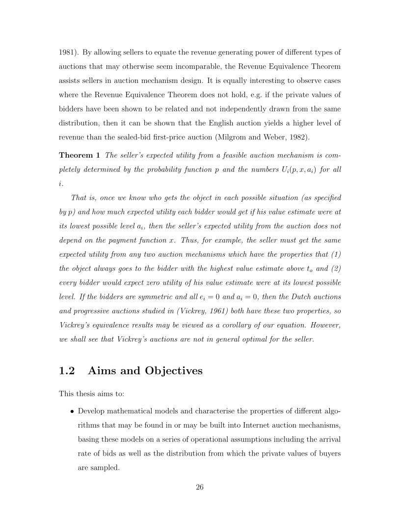
Further to this, there are other independent properties that can be incorporated

when designing an auction (Parsons et al., 2011). These other properties are listed

below and a taxonomy of auctions is shown in Figure 1-4.

• Combinatorial: auctions that are combinatorial see multiple heterogeneous

goods auctioned together.

• Dimensionality: in a singularly-dimensional auction, the bid is completely

defined by the price of the lot, whereas in a many-dimensional auction, the bid

23

Bid 1

EnglishAuction

Bid 2

Bid 3

Bid n

.

.

.

max (bid i)(1)i

Figure 1-1: English auction process.

Bid 1

ReverseAuction

Bid 2

Bid 3

Bid n

.

.

.

min (bid i)(1)i

Figure 1-2: Reverse auction process.

may be a function of other attributes such as the timely delivery of the lot or

the length and amount of the insurance contract taken out on that lot.

• Sidedness: in a one-sided auction, bidders are either all sellers or all buyers.

In a two-sided auction, bids are submitted by both buyers and sellers and these

are matched by the auctioneer.

In fact, in auctions without time restrictions, the English and the sealed-bid

second-price auctions have been shown to be equivalent, while the Dutch and the

24

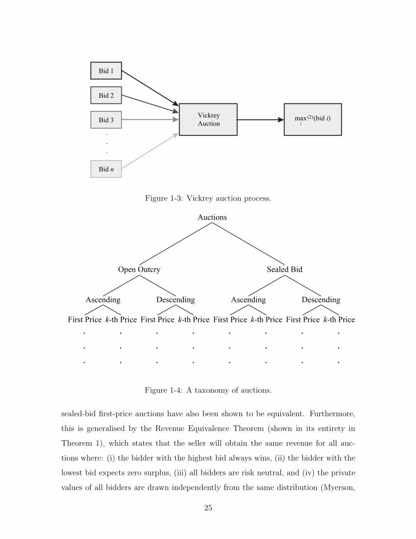
Bid 1

VickreyAuction

Bid 2

Bid 3

Bid n

.

.

.

max (bid i)(2)i

Figure 1-3: Vickrey auction process.

Auctions

Open Outcry Sealed Bid

DescendingAscending DescendingAscending

First Price k-th Price First Price k-th Price First Price k-th Price First Price k-th Price...

.

.

.

.

.

.

.

.

.

.

.

.

.

.

.

.

.

.

.

.

.

Figure 1-4: A taxonomy of auctions.

sealed-bid first-price auctions have also been shown to be equivalent. Furthermore,

this is generalised by the Revenue Equivalence Theorem (shown in its entirety in

Theorem 1), which states that the seller will obtain the same revenue for all auc-

tions where: (i) the bidder with the highest bid always wins, (ii) the bidder with the

lowest bid expects zero surplus, (iii) all bidders are risk neutral, and (iv) the private

values of all bidders are drawn independently from the same distribution (Myerson,

25

1981). By allowing sellers to equate the revenue generating power of different types of

auctions that may otherwise seem incomparable, the Revenue Equivalence Theorem

assists sellers in auction mechanism design. It is equally interesting to observe cases

where the Revenue Equivalence Theorem does not hold, e.g. if the private values of

bidders have been shown to be related and not independently drawn from the same

distribution, then it can be shown that the English auction yields a higher level of

revenue than the sealed-bid first-price auction (Milgrom and Weber, 1982).

Theorem 1 The seller’s expected utility from a feasible auction mechanism is com-

pletely determined by the probability function p and the numbers Ui(p, x, ai) for all

i.

That is, once we know who gets the object in each possible situation (as specified

by p) and how much expected utility each bidder would get if his value estimate were at

its lowest possible level ai, then the seller’s expected utility from the auction does not

depend on the payment function x. Thus, for example, the seller must get the same

expected utility from any two auction mechanisms which have the properties that (1)

the object always goes to the bidder with the highest value estimate above to and (2)

every bidder would expect zero utility of his value estimate were at its lowest possible

level. If the bidders are symmetric and all ei = 0 and ai = 0, then the Dutch auctions

and progressive auctions studied in (Vickrey, 1961) both have these two properties, so

Vickrey’s equivalence results may be viewed as a corollary of our equation. However,

we shall see that Vickrey’s auctions are not in general optimal for the seller.

1.2 Aims and Objectives

This thesis aims to:

• Develop mathematical models and characterise the properties of different algo-

rithms that may be found in or may be built into Internet auction mechanisms,

basing these models on a series of operational assumptions including the arrival

rate of bids as well as the distribution from which the private values of buyers

are sampled.

26

• Construct and run simulation experiments in the context of the mathematical

models, checking the validity of the mathematical models and using the same

assumptions.

• Scrape data from real-world auction websites and evaluate the extent to which

the mathematical model agrees with the data. The information derived from

this analysis is then used for parameter tuning in order to align the mathemat-

ical model with real-world data.

1.3 Contributions

Internet auctions exhibit characteristics which are not often shared with conventional

auctions, e.g. auctions of fixed duration which encourage sniping (whereby bidders

submit their bids moments before the close of an auction thereby preventing other

bidders from submitting counter-bids), the acceptance of multiple bids in a single

auction, and a maximum threshold whereby the auction will terminate at that price

point. Due to lack of regulation, the size of the market and the volume of bid-

ders and sellers, Internet auctions are better suited to incorporating algorithms of

increased complexity as opposed to the more established procedures at traditional

auction houses. For example, while eBay runs what essentially amounts to an En-

glish auction with a fixed duration, Swoopo runs what is known as a bidding fee

auction, where each bid incurs a fee and also extends the length of the auction by a

short amount (10–20 seconds).

This report provides a mathematical analysis of the characteristics and the prop-

erties of these different and unconventional types of Internet auctions using a series of

operational assumptions which characterise the arrival rate of bids, as well as the dis-

tribution from which the private values of buyers are sampled. From this, closed-form

expressions of several key performance metrics are determined, including the average

selling price in a given auction, as well as the average auction duration. In cases

where a seller may be selling a commodity and auctions repeat themselves with the

same items for sale multiple times, the income per unit time may also be quantified.

27

Having such analysis will pave the way for the development of optimum and

dominant strategies on the part of both the buyer and the seller and an understanding

of how the sensitivity of different auction parameters affect the income and length of

an auction will aid auction design. A seller can decide the optimal type of auction

to host given his/her aims, with the performance of the chosen auction able to be

measured with different metrics in accordance to the specific aims.

1.4 Publications

• Leung, Timothy L. Y., and Knottenbelt, W. J. (2012). Comparative Evaluation

of Independent Private Values Distributions on Internet Auction Performance.

International Journal of E-Entrepreneurship and Innovation (IJEEI), 1(3):59–

71. London, UK.

• Leung, Timothy L. Y., and Knottenbelt, W. J. (2011). Consumer-to-consumer

Internet Auctions. International Journal of Online Marketing (IJOM), 1(3):17–

28. London, UK.

• Leung, Timothy L. Y., and Knottenbelt, W. J. (2011). The Effect of Private

Value on E-Auction Revenues. In Proceedings of the 2011 International Con-

ference on Digital Enterprise and Information Systems (DEIS 2011). London,

UK.

• Leung, Timothy L. Y., and Knottenbelt, W. J. (2011). Global B2C and C2C

Online Auction Models. In Proceedings of the 2011 Annual Conference on In-

novations in Business and Management (CIBMP). London, UK.

• Leung, Timothy L. Y., and Knottenbelt, W. J. (2011). Stochastic Modelling and

Optimisation of Internet Auction Processes. In Proceedings of the 6th Workshop

on Practical Applications of Stochastic Modelling (PASM 2011). Karlsruhe,

Germany.

28

• Sakellari, Georgia, and Leung, Timothy L. Y., and Gelenbe, Erol. (2011).

Auction-based Admission Control for Self-Aware Networks. In Proceedings of

the 26th International Symposium on Computer and Information Sciences (IS-

CIS 2011). London, UK.

• Leung, Timothy L. Y., and Knottenbelt, W. J. Analysis of Internet Auction

Processes and Mechanisms. ACM Transactions on Internet Technology. (To be

submitted).

1.5 Thesis Outline

In Chapter 2, existing literature that addresses the current landscape of Internet

auctions is reviewed. This is divided into sections detailing Internet Auction Charac-

teristics and Applications, Internet Auction Behaviour, and the Stochastic Modelling

of Auction Processes.

Chapter 3 presents the algorithms that represent a variety of different Internet

auction mechanisms, analysing them in a stochastic framework. In particular, an

examination of the metrics, average auction duration and the average offer accepted,

are analysed for each auction mechanism.

Chapter 4 extends the theory in the previous chapter to additional types of auc-

tions found on the Internet. These include the Vickrey and reverse auction algorithms.

A similar approach is taken to that in Chapter 3, with the metrics, average auction

duration and the average offer accepted, being analysed for each auction mechanism.

Chapter 5 conducts surplus analysis and uses allocative efficiency in evaluating

how Internet auctions perform.

Chapter 6 conducts experimental validation for the algorithms detailed in Chap-

ters 3 and 4. Simulation experiments are performed, and comparisons are made

between the theoretical predictions and experimental observations. Furthermore,

real-world data scraped from eBay is used to compare with the model assumptions.

Chapter 7 deals with generalisations and extensions of the auction algorithms and

outlines the stochastic behaviour of private values and auction performance and the

29

invariance of distribution on private values. In addition, generalisation of the results

to non-homogeneous Poisson bid arrival is undertaken.

The thesis concludes with Chapter 8 where a list of thesis achievements are given

in addition to details on the applications of the work that constitutes the thesis and

directions for future work.

30

Chapter 2

Literature Review

2.1 Introduction

Internet auctions have begun to pervade large sections of the Internet economy and

there is an increasing amount of literature in this field. As a first step, we provide

a detailed comparison of the characteristics of Internet auctions which are often not

shared by conventional auctions in Table 2.1.

2.2 Internet Auction Characteristics and Applica-

tions

There has been substantial work done on auctions (see Figure 2-1), with several books

written on the topic (Cramton et al., 2006; Klemperer, 2004; Krishna, 2002; Milgrom,

2004). As a branch of game theory, auctions have been given the classification, D44,

by the Journal of Economic Literature. Though parallel in many ways, the volume of

literature on Internet auctions, however, is significantly less. It is important to draw

precise distinctions between traditional and Internet auctions in order to determine

which aspects of auction theory are applicable to which.

The Independent Private Values model is often associated with auctions (Parsons

et al., 2011). The characteristics of this model include the assumptions of privacy and

31

Internet Auctions Conventional Auctions

Asynchronous; bidders need not be at thesame place at the same time

Synchronous

Global competition across national bound-aries

No competition across national boundaries

Vickrey auctions dominant Tend to be first-price auctionsCan have absolute pre-determined end-time

Pre-determined fixed end-time usually notacceptable

Can run for days or weeks Usually run for no more than minutes orhours

Concealed information; highest bid notknown

Often without concealed information —highest bid known

Sniping No snipingBuy-It-Now (BIN) option common Buy-It-Now option uncommonCan support arbitrarily complex auctionrules and algorithms (e.g. Timeshift, Re-ject without recall)

Unable to support such complexity

Seller Ratings; a key consideration Seller Ratings — largely unimportantLarge-scale shilling possible through sellerssystematically creating bidding accounts

Large-scale shilling not feasible

Timely submission of bids depends on net-work speed and reliability

No such dependency

Bidders may participate in several auctionssimultaneously (via Desktops, Notebooks,Mobile Phones etc.)

Usually not possible or with difficulty; notthe same degree of monitoring or control

Proxy bidding widely used Proxy bidding not widely usedBidders need to create accounts first and“reveal” their identity

Mystery bidders may sometimes just turnup without revealing their identities

Statistically determined or event triggeredrandom end-time may be adopted

Random end-time usually not acceptable

Increasingly dominant as a mechanism fordifferent types of business and commercialtransactions

Auctions not extensively used for conven-tional business and commercial transac-tions and likely to remain so

Inspection of items not usually possible Inspection of items usually possibleMultiple channels of delivery Usually a single channel of deliverySellers can be a company A company selling normal items through

auctions is not cost-effectiveIndividuals can make systematic sales andprofits using auctions without needingto set up a company (i.e. dedicated e-commerce site)

Hard for individuals to do regular businessusing only auctions

Table 2.1: Comparison between Internet auctions and conventional auctions.

32

independence where the value of the commodity in question is private to the individual

buyers, and that different buyers do not know the values other buyers attach to the

commodity. In addition, these values are drawn from a common distribution which

is known to the buyers. In probabilistic terms, this essentially amounts to a series

of values which are independent and identically distributed. A common distribution

used is the uniform distribution (Katok and Kwasnica, 2008). In our subsequent

analysis, we shall follow the independent private values model using the uniform

distribution.

The online auction website, eBay, is a popular and recent implementation of the

auction mechanism. It is classed as a consumer-to-consumer (C2C) auction and it

runs open-bid second-price auctions that are of a fixed length. Due to its fixed

length, eBay auctions are susceptible to sniping, which see bidders submit their bids

moments before the close of an auction preventing other bidders from submitting

counter-bids (Ockenfels and Roth, 2006). While this is seen to be problematic, eBay

has always maintained the policy that a bidder should bid his private value. Since

the winner pays the second price, there is little reason for a bidder to shade his bid.

In order to counteract sniping, other online auction websites, such as Amazon, have

employed auctions with a soft close, automatically extending the length of the auction.

The investigation of different types of auction terminations has been undertaken in

Ockenfels and Roth (2002), where it is found that late bidders in eBay-style auctions

tend to be associated with highly experienced bidders, whereas those of the Amazon-

type tend to be relatively inexperienced bidders. In Bajari and Hortacsu (2003), it is

found that sniping often leads to winning, and it observes that many sellers tend to

set the starting bid price unrealistically low to stimulate bidder participation.

In Kaghashvili (2009), the mechanism of online timeshift auctions is proposed,

whereby auctions are qualitative modifications of the existing popular auctions with

items offered for a fixed time period. Conducting a standard timeshift auction com-

prises of several steps: i) the seller defines an auction length and a specific point

during the auction where the auction transitions to the timeshift interval before ter-

minating, ii) following the highest bidder who had placed at least a single bid before

33

the transition to the timeshift interval, obtains the item. For B2C online auctions,

the analysis of their design, and the optimal design of online auction channel have

been studied in Bapna et al. (2002, 2003).

Experimental

Katok, E. and Kwasnica, A (2008) Kauffman, R. and Wood, C. (2005) Lucking-Reiley, D.

(1999) Lucking-Reiley, D., Bryan, D., Prasad, N., and Reeves, D. (2007) Vragov, R. (2010) Wang, S., Jank,

W., and Shmueli, G. (2008) Wenyan, H. and Bolivar, A.

(2008)

Stochastic Analysis

Gelenbe, E. (2009) Guo, X. (2002) Russo, R.,

Shyamalkumar, N., and Shmueli, G. (2008)

Shmueli, G., Russo, R., and Jank, W.

(2007)

Economic Analysis

Bapna, R., Jank, W., Shmueli, G., and Hyderabad, G. (2008) Cramton, P., Shoham, Y., and

Steinberg, R. (2006) Klemperer, P. (2004) Krishna, V. (2002)

McAfee, R. and McMillan, J. (1987) Milgrom, P. (2004) Milgrom, P. and Weber, R.

(1982) Vickrey, W. (1961)

Analytical

Chen, H. and Li, Y. (2000)

Behavioural

Bajari, P. and Hortacsu, A. (2003) Haruvy, E., Popkowski Leszczyc, P., Carare, O., Cox, J., Greenleaf, E., Jank, W., Jap, S.,

Park, Y., and Rothkopf, M. Ockenfels, A. and Roth, A. (2002) Ockenfels, A. and

Roth, A. (2006)

Bapna, R., Goes, P., and

Gupta, A. (2003) Bapna, R., Goes,

P., Gupta, A., and Jin, Y.

(2004) Bapna, R., Goes, P.,

Gupta, A., and Karuga, G.

(2002)

Market-based

Dass, M. and Reddy, S. (2008) Friedman, D. (1993) Ran, S.

(2003)

Auction Applications

Huang, S. (2005) Lin, W.-Y., Lin, G.-Y., and Wei, H.-Y. (2010) Liu, Y.,

Goodwin, R., and Koenig, S. (2003)

Mullins, C. L. (2008) Niu, J.,

Cai, K., McBurney, P., and

Parsons, S. (2009) Po- dobnik, V., Trzec, K., and Jezic, G. (2006) Ran, S. (2003)

Shehory, O. and Sturm, A. (2001) Yi, X. and Siew, C. (2001) Zambonelli,

F., Jennings, N., and Wooldridge, M. (2003)

Figure 2-1: Venn diagram classification of literature covered in this literature review.

The user of auctions as a market mechanism has also been studied in various

e-business and Web services contexts (Chen and Li, 2000; Ran, 2003; Huang, 2005),

often for allocating different types of resources with different policies for pricing. In

Huang (2005), a progressive resource allocation scheme which is the continuous ver-

sion of the generalised Vickrey auction is used, where the auction mechanism is built

34

into the service sharing prototype so that users and auctioneers rely on the software

agents to exchange information in a distributed environment. More recent Internet

auction applications include Cloud computing resource allocation (Lin et al., 2010),

as typified by Amazon’s EC2 cloud computing service. The EC2 employs a continu-

ous double auction (CDA) for cloud server space, which they label “Spot Instances”,

and which has been analysed within a framework that simulates dynamic demand

through the peak/off-peak concept. In a recent patent (Mullins, 2008), Microsoft has

extended this use of double auctions to incorporate different types of decentralised

computing resources, which is partitioned into a two-tier pricing structure that ac-

counts for peak and off-peak traffic, with the discounted price of the latter reflecting

an increased risk of latency and network outage. In Lin et al. (2010), a dynamic auc-

tion mechanism for solving the allocation problem of computation capacity in cloud

computing is proposed, which makes use of second-price auctions to regulate com-

putational resource efficiency and to ensure a reasonable level of profit for the CSP

(Cloud Service Provider).

2.3 Internet Auction Behaviour

Studies of Internet auction bidding behaviour have been undertaken in Ockenfels and

Roth (2002, 2006); Wenyan and Bolivar (2008) In Wenyan and Bolivar (2008), differ-

ent properties of online auctions such as consumer surplus, sniping, bidding strategy

and their interactions are studied, and a significant correlation between sniping and

surplus ratios is found. It also examines the efficiency of online auctions, where Pareto

efficiency is used as the optimality criterion. In Ockenfels and Roth (2006), it is sug-

gested that the strategic advantages of sniping are eliminated or severely eroded in

auction mechanisms that apply an auction extension rule, and that there is noticeable

difference between sniping on eBay and Amazon in proportion to user experience.

Experimental studies of Internet auction behaviour have been undertaken in Lucking-

Reiley (1999); Vragov (2010); Katok and Kwasnica (2008). In Katok and Kwasnica

(2008), it concentrates on the Dutch auction and first-price sealed bid auction for-

35

mats, using laboratory experiments and human subjects, where values are drawn from

the uniform distribution between 0 and 100, focusing primarily on the effect of clock

speed on seller’s revenue. In Vragov (2010), laboratory experiments with human sub-

jects are also conducted, and the operational efficiency of Internet auctions is studied.

Collusion behaviour such as shilling, in which the seller plays a part in the bidding

process, is studied in Kauffman and Wood (2005), where two types of shilling strate-

gies are examined, these deploy competitive bidding and reserve price mechanism and

each of these exhibits a characteristic pattern of behaviour. While an auction can

be defined as a market institution whereby offers are made only by the buyers, i.e.

bids, or only by the sellers, i.e. asks, a double auction is one where both buyers and

sellers are able to make offers (Friedman, 1993). Viewing the interlinking relationship

between bidders and sellers as networks is proposed in Dass and Reddy (2008), and

the competitions in auctions is investigated in Haruvy et al. (2008). Price variation

characteristics and consumer surplus are studied in Bapna et al. (2008); Jank et al.

(2006). The use of various types of curves for fitting price data for Internet auctions

have been proposed in Hyde et al. (2007), in which monotone splines and beta func-

tions are used. Empirical investigations of eBay auctions have also been undertaken

in Lucking-Reiley et al. (2007) where the auction of coins is conducted. This makes

use of regression models to estimate the price of items and examines the influence of

seller ratings (which measures the reliability and services provided by the seller) on

the final price. It has also found that the effect of positive and negative ratings is not

symmetrical, with the latter having a much greater (adverse) influence on the price.

It also suggests that longer auctions tend to have a beneficial effect in achieving a

higher price. Moreover, in Dellarocas and Wood (2008), it was found that there is

a reluctance on the part of users to give negative feedbacks compared with giving

positive feedbacks. The K-means clustering algorithm has been employed in Bapna

et al. (2004) which classifies bidders into five categories based on factors such as entry

time, number of bids placed, and exit time. It also examines the use of automated

agents in carrying out bidding as well as the different experience levels of bidders. The

use of analogies from physics to study price movements have been applied in Hyde

36

et al. (2007); Jank et al. (2008); Wang et al. (2008), which make use of the concepts

of price-velocity to characterise the dynamics of price changes and may subsequently

be exploited to produce forecasts.

2.4 Stochastic Modelling of Auction Processes

While the majority of the literature in the previous section considered auctions in

their entirety, it is useful to look at cases where the bids are separated from each

other and arrive following a certain distribution. A stochastic number of bidders is

studied in McAfee and McMillan (1987), where first-price sealed-bid auctions having

constant absolute risk aversion is analysed. As a result of the stochastic analysis,

the authors conclude that the seller should conceal the number of bids in order to

maximise the selling price. Stochastic models of bid arrival characteristics are studied

in Shmueli et al. (2007); Russo et al. (2008), where the so-called BARISTA (Bid

ARrivals InSTAges) model that makes use of non-homogeneous Poisson process is

proposed. The probabilistic and statistical properties of these models are analysed

and studied and the usefulness of these models for auction modelling is illustrated

and discussed.

An interesting Internet auction mechanism is proposed in Guo (2002). It considers

a seller who sets the lowest acceptable price for an item without revealing it, with

bidders arriving at different times with their bids. If a bid is lower than the set

lowest acceptable price, the seller immediately rejects the bid. However, if a bid is

higher than the set lowest acceptable price, then the seller faces the decision of either

accepting this bid or rejecting it and moving on to the next bidder, with the hope

of achieving a higher price. In the latter case, it is assumed that the rejected bid

disappears, never to return. Assuming that the seller is allowed to make a choice at

any time, the goal is to maximise the sellers expected return by choosing the best bid.

The situation is represented as an optimal stopping problem, and using techniques

from convex analysis, an explicit solution that yields a simple algorithm for the seller

is obtained.

37

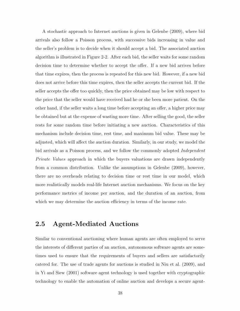
A stochastic approach to Internet auctions is given in Gelenbe (2009), where bid

arrivals also follow a Poisson process, with successive bids increasing in value and

the seller’s problem is to decide when it should accept a bid. The associated auction

algorithm is illustrated in Figure 2-2. After each bid, the seller waits for some random

decision time to determine whether to accept the offer. If a new bid arrives before

that time expires, then the process is repeated for this new bid. However, if a new bid

does not arrive before this time expires, then the seller accepts the current bid. If the

seller accepts the offer too quickly, then the price obtained may be low with respect to

the price that the seller would have received had he or she been more patient. On the

other hand, if the seller waits a long time before accepting an offer, a higher price may

be obtained but at the expense of wasting more time. After selling the good, the seller

rests for some random time before initiating a new auction. Characteristics of this

mechanism include decision time, rest time, and maximum bid value. These may be

adjusted, which will affect the auction duration. Similarly, in our study, we model the

bid arrivals as a Poisson process, and we follow the commonly adopted Independent

Private Values approach in which the buyers valuations are drawn independently

from a common distribution. Unlike the assumptions in Gelenbe (2009), however,

there are no overheads relating to decision time or rest time in our model, which

more realistically models real-life Internet auction mechanisms. We focus on the key

performance metrics of income per auction, and the duration of an auction, from

which we may determine the auction efficiency in terms of the income rate.

2.5 Agent-Mediated Auctions

Similar to conventional auctioning where human agents are often employed to serve

the interests of different parties of an auction, autonomous software agents are some-

times used to ensure that the requirements of buyers and sellers are satisfactorily

catered for. The use of trade agents for auctions is studied in Niu et al. (2009), and

in Yi and Siew (2001) software agent technology is used together with cryptographic

technology to enable the automation of online auction and develops a secure agent-

38

Auction-in-progress

Inter-arrivalTime of Bid

RandomDecision Time

AuctioneerRest Time

Figure 2-2: Gelenbe auction algorithm.

mediated online auction framework (see Figure 2-3). In the proposed framework,

an online auctioneer generates an auction agent which acts as a mobile auctioneer

traversing a list of online bidders, asking and collecting bids of each round to the

online auctioneer. From the bid information so collected, the online auctioneer spec-

ifies a new minimum bid and sends out the software agent again. This process is

repeated until a minimum bid remains unchanged for three consecutive times, af-

ter which the auctioneer would broadcast the auction outcome. Generalisation of

such agent-mediated auctioning mechanism is indicated in Zambonelli et al. (2003)

in which both buyers and sellers also employ agents in a multi-agent environment to

achieve the overall application goal.

In Shehory and Sturm (2001), the implementation of an auction agent is de-

scribed, which participates and bids in web-based auctions on behalf of its user. The

user provides the agent with relevant details of product, price and bidding strategy

before activating the agent. After being activated, the agent enters the auction site,

locates the specific product, and monitors the site. The agent terminates its auction

activity either when its buying strategy requires withdrawal or when the auction fin-

ishes. In Das et al. (2001), a series of laboratory experiments that employs human

subjects to interact with software bidding agents in continuous double auctions are de-

scribed, and it is found that agents consistently obtain significantly larger gains from

39

Bidder

Auctioneer

BidderBidder

Bidder

Bidder

Agent

AgentAgent

Agent

Agent

Agent

Figure 2-3: Illustration of the Agent-mediated online auction framework.

trade than their human counterparts, and that unexpected non-equilibrium trading

is observed in such systems. In Podobnik et al. (2006), mediation between service

requester’s agents and sellers service provider’s agents is studied, in which enables

provider agents to dynamically and autonomously advertise semantic descriptions of

available services through an auction model, called the Semantic Pay-Per-Click Agent

(SPPCA) auction. Requester agents then use the advertised services to discover ap-

propriate services. Then, information regarding the actual performance of service

providers is considered in conjunction with the prices bid by service provider’s agents

in the SPPCA auction before a final set of advertised services is then chosen and

proposed to the buyer agent as an answer to its request.

In Liu et al. (2003) a theory for auction agents forming part of a supply-chain man-

agement system combining concepts from auction theory, utility theory, and dynamic

programming is proposed. It employs results from utility theory to obtain the opti-

mal bidding strategy for risk-averse auction agents, both for first- and second-price

sealed-bid auctions in the symmetric independent private values model, in addition

40

to using dynamic programming techniques to integrate the resulting auction agents

with a production-planning system. It also makes use of simulations in combining

the auction and production-planning system to obtain crude approximations of the

competitor’s valuations distributions of the auctioned item. This theory aims to pro-

vide a framework for building more powerful auction agents geared to highly complex

decision situations. In our study, the actual auction implementation mechanism may

or may not make use of agents to achieve the desired goal. Using agents, however,

may have the advantage of saving significant human efforts, especially when the auc-

tion takes place at times when the participating parties are unavailable. Similar to

the study Liu et al. (2003), we also make use of simulation experiments, but unlike

those, we also develop mathematical analysis of the different auction algorithms which

mostly leads to closed-form results.

41

Chapter 3

Analysis of Auction Algorithms

This chapter contains the algorithms of a number of key auctions which differ from

one another in a significant way. In the analyses that follow, both in this current

chapter and the next, the different Internet auction algorithms may be categorised

according to their properties and characteristics:

1. First-price Forward Auctions with Fixed Duration (Algorithms I, III)

2. First-price Forward Auctions with Variable Duration (Algorithms II, IV, V)

3. Vickrey Auctions with Fixed Duration (Algorithms VI, VIII)

4. Vickrey Auctions with Variable Duration (Algorithms VII, IX, X)

5. Reverse Auctions with Fixed Duration (Algorithms XI, XIII)

6. Reverse Auctions with Variable Duration (Algorithms XII, XIV, XV)

Specifically, this chapter examines the cases of the fixed-time first-price forward

auction, which is similar to eBay, the first-price forward auction with variable dura-

tion, which is similar to the auctions that occur in auction houses such as Christie’s

and Sotheby’s, the cases where there is a maximum threshold termination, i.e. the

auction is terminated on reaching a specific bid level, and the case where the auction

is terminated on reaching a specific number of bids.

43

The purpose of this chapter and the next is to deduce, given the simple set of

assumptions detailed below, the closed-form solutions to a number of key metrics

that can be used to compare the different auction types. These key metrics include

the average auction income as well as the average auction duration, and in cases

where possible, the average auction income per unit time.

While these closed form solutions are deduced using theoretical methods, Chapter

6 gathers real-world data from eBay auctions and tests the model with the collected

data, computing how closely they compare with each other, and in so doing, deter-

mining how well the theoretical formulas describe real-world behaviour.

Internet auction mechanisms take on a variety of forms. Many of them are forward

auctions, e.g. http://www.ebay.com, such as the English and Vickrey auctions, while

others may be reverse auctions, e.g. http://www.oltiby.com. There are auctions

that are of fixed duration, and there are those that allow an auction to terminate

prematurely when a high enough bid is received. Usually only a single bid is accepted

in each auction, but there also exist auctions that allow the acceptance of multiple

bids in an auction, e.g. Google AdWords.

As in Gelenbe (2009), bids are assumed to arrive over time in a Poisson manner

with rate λ, and that the bids Qk are ascending ordered values taken from the

uniform distribution over the interval (0, L). The latter is a commonly-used distri-

bution in auction analysis (Katok and Kwasnica, 2008). This property is further

discussed in Chapter 7. If there are N bids, these ordered values are denoted by

Q(1) < Q(2) < . . . < Q(N).

3.1 Auction Algorithm I: Fixed-time First-price

Forward Auction

A forward auction is an auction where buyers compete for lots and the price increases

as time passes. An example of this type of auction is eBay. In this algorithm,

the auction time is assumed to be fixed with duration T . Let N be the number of

44

bids received, such that the largest bid Q(N) received over the time interval (0, T ) is

accepted. Each bid comes at a certain time t, with a bid value of R, from a user with

a specific bidder_id. A high value for T will produce a larger average accepted bid

but the duration of the auction will be longer. For practical and meaningful operation

of the auction, T should be significantly greater than the mean bid inter-arrival time,

1/λ, i.e. T 1/λ . At the close of the auction, the maximum bid Q(N) is accepted

(see Algorithm I).

Algorithm 1 Fixed-time first-price forward auction.

Require: T > 0Ensure: L > 0 and accept id 6= nullaccept id← nullclock ← 0L← 0while clock < T do

while newbid(t, R, bidder id) doclock ← clock + tif clock < T and R > L thenL← Raccept id← bidder id

end ifend while

end whilereturn L, accept id

From the results of order statistics (Barry C. Arnold et al., 2008), it can be shown

that the conditional income per auction is

E[Q(N)|Number of bids = N ] =NL

N + 1. (3.1)

Since,

dE[Q(N)|Number of bids = N ]

dN=

L

(N + 1)2> 0,

as the number of bids N increases, the corresponding average income per auction will

also increase. Thus, when the bid arrival λ rate is high, the corresponding average

income per auction is likewise be expected to be high. To determine the average

45

income E[Q(N)

], the condition on N is removed in Equation 3.1 using the Poisson

probabilities, i.e.

E[Q(N)

]=

∞∑N=1

NL

N + 1× e−λT (λT )N

N !

=∞∑N=1

[L− L

N + 1

]× e−λT (λT )N

N !

=∞∑N=1

L× e−λT (λT )N

N !−∞∑N=1

L

N + 1× e−λT (λT )N

N !

= L(1− e−λT

)− Le−λT

λT

∞∑N=1

(λT )N+1

(N + 1)!

= L(1− e−λT

)− Le−λT

λT

(eλT − 1− λT

). (3.2)

The term N = 0 is omitted above, since the income is zero upon N = 0. This

gives an average income per auction of

E[Q(N)

]=

L

λT

(λT + e−λT − 1

), (3.3)

and an income rate, or income per unit time, of

L

λT 2

(λT + e−λT − 1

). (3.4)

Figure 3-1 shows E[Q(N)

]for different values of λ for L = 100, and T = 5, 10, 15.

In the case where T = 10, the increase in bid rate up to λ = 4 produces a rather

steep average auction income improvement. There seems to be a critical bid rate at

around λ = 6, above which the improvement in income becomes less pronounced.

Figure 3-2 shows E[Q(N)

]/T , or the income rate, for different values of λ for

L = 100, and T = 5, 10, 15. In the case where T = 10, the increase in bid rate up

to λ = 1 produces a rather marked increase in auction income rate. There seems to

be a critical bid rate at around λ = 2, above which the increase in auction income

rate slows down. Moreover, the income rate drops as T increases, and the drop is

much more significant for smaller values of T : the drop is much greater from T = 5

46

0 2 4 6 8 10

60

70

80

90

Bid Rate

Income

T = 5.0T = 10.0T = 15.0

Figure 3-1: Average auction income of fixed-time first-price forward auction.

to T = 10 than from T = 10 to T = 15.

0 2 4 6 8 10

5

10

15

20

Bid Rate

Income Rate

T = 5.0

T = 10.0

T = 15.0

Figure 3-2: Average auction income rate of fixed-time first-price forward auction.

Differentiating the auction income with respect to T , yields

dE[Q(N)

]dT

=L

λT 2

[1− 1 + λT

eλT

].

47

Since, λT > 0, and

eλT = 1 + λT +(λT )2

2!+

(λT )3

3!+ . . . , (3.5)

the inequality (1 + λT ) < eλT holds, so that (1 + λT )/eλT < 1, and thus

[1− 1 + λT

eλT

]> 0.

Consequently,

dE[Q(N)

]dT

> 0.

Thus, the auction income can be raised by increasing the auction duration. Sim-

ilarly, differentiating the auction income with respect to λ and by similar argument

using Equation 3.5,

dE[Q(N)

]dλ

=L

λ2T

[1− 1 + λT

eλT

]> 0.

Thus, the auction income can also be augmented by increasing the incoming rate

of bids.

3.2 Auction Algorithm II: Variable-time First-price

Forward Auction with Fixed Inactivity Win-

dow

Here, unlike Algorithm I, the auction will terminate when there is no bid arrival for

a fixed window of length α. On termination, the largest bid received will be accepted

(see Algorithm II).

The fixed inactivity window α may be adjusted, and for meaningful operation,

should not be significantly smaller than the mean bid inter-arrival time; a high value

48

Algorithm 2 Variable-time first-price forward auction with fixed inactivity window.

Require: α > 0Ensure: L > 0 and accept id 6= nullaccept id← nullL← 0loop

while newbid(t, R, bidder id) doif t < α then

if R > L thenL← Raccept id← bidder id

end ifelse

return L, accept idend if

end whileend loop

for α will produce a higher income but the auction will take longer. Unlike Algo-

rithm I, in which the auction duration is always bounded by T , here, it is possible

for the auction duration to go on for an indefinite period without a predictable end

point. In particular, if the average bid inter-arrival time 1/λ is significantly less than

α, i.e. α 1/λ, or λα 1, then there is little chance of having an interval of length

α without any arrival.

Let V (α) be the average waiting time from the beginning of the auction to the

(beginning of the) first occurrence of an inter-arrival time interval of greater than α

(i.e. excluding the time interval α itself). If the first arrival interval is less than α,

which happens with probability (1− e−λα), then the process effectively starts all over

again, except for any time penalty incurred, i.e.

V (α) =∫ α

0λte−λtdt+ (1− e−λα)V (α), (3.6)

where the first term represents the waiting time penalty for the first bid arrival av-

eraged over an inter-arrival interval of less than α. Solving for V (α), Equation 3.6

49

becomes

V (α) = eλα∫ α

0λte−λtdt = eλα

[1− e−λα(λα + 1)

λ

]=eλα − (λα + 1)

λ

This gives an average auction duration of τα = α + V (α), i.e.

τα =eλα − 1

λ. (3.7)

It can be seen that

dταdα

= eλα > 0,

so that τα grows as α increases. Figure 3-3 shows how τα varies with λ for α = 1, 2

and 3. It can be seen that τα increases relatively gradually for small values of λ, but

accelerates for large values. As the bid rate increases, there is reduced chance of a

no-bid interval occurring, which lengthens the auction, and the difference between

α = 1 and α = 3 also becomes more pronounced as λ→ 2.

0 1 2

40

80

120

160

Bid Rate

Duration

α = 1.0α = 2.0

α = 3.0

Figure 3-3: Average auction duration of variable-time first-price forward auction withfixed inactivity window.

To determine the average income E[Q(N)

], the condition on N in Equation 3.1

is removed. Unlike the fixed-time case where Poisson probabilities could be used,

50

however, the probability mass function for N must first be determined. Denoting the

inter-arrival times by Tk, the number of bids is N if

T1 < α, T2 < α, . . . , TN < α, TN+1 ≥ α

Now, the probability of Tk < α is 1 − e−λα and the probability of TN+1 ≥ α is

e−λα, and since the sequence Tk is independent,

Pr[T1 < α, T2 < α, . . . , TN < α, TN+1 ≥ α] = (1− e−λα)N × e−λα. (3.8)

Thus,

E[Q(N)

]=

∞∑N=1

NL

N + 1× (1− e−λα)Ne−λα

=∞∑N=1

[L− L

N + 1

]×(1− e−λα

)Ne−λα

=∞∑N=1

L(1− e−λα

)Ne−λα − Le−λα

(1− e−λα)

∞∑N=1

(1− e−λα

)N+1

N + 1

= L(1− e−λα

)− Le−λα

(1− e−λα)

∞∑N=1

(1− e−λα

)N+1

N + 1(3.9)

From the logarithmic series,

∞∑N=1

θN

N= − log(1− θ), (3.10)

and letting θ = 1− e−λα, from Equation 3.9,

E[Q(N)

]= L

(1− e−λα

)− Le−λα

1− e−λα

∞∑N=1

(1− e−λα

)NN

− (1− e−λα)

= L(1− e−λα

)− Le−λα

1− e−λα[− log

(e−λα

)−(1− e−λα

)],

51

which gives,

E[Q(N)

]= L

(1− e−λα

)− L

eλα − 1

[λα + e−λα − 1

].

On simplification,

E[Q(N)

]=

L

eλα − 1

[eλα − λα− 1

]= L

[1− λα

eλα − 1

]. (3.11)

Combining with Equation 3.7, this becomes

E[Q(N)

]= L

[1− α

τα

]. (3.12)

Figure 3-4 gives the average auction income as a function of λ for α = 1, 2 and 3.

From the graph, income differences tend to narrow for high values of α.

0 1 2

20

40

60

80

Bid Rate

Income

α = 1.0

α = 2.0α = 3.0

Figure 3-4: Average auction income of variable-time first-price forward auction withfixed inactivity window.

Differentiating the auction income with respect to α, yields

dE[Q(N)

]dα

=λL

[eλα(λα− 1) + 1

](eλα − 1)2 .

For the running of the auction to be meaningful, there must be an average of at

52

least one bid arrival per interval of length α, i.e. λα ≥ 1, so that

dE[Q(N)

]dα

=λL

[eλα(λα− 1) + 1

](eλα − 1)2 > 0.

This shows that the auction income can be increased by augmenting the inactivity

window, α. Similarly, differentiating the auction income with respect to λ and by

similar argument,

dE[Q(N)

]dλ

=αL

[eλα(λα− 1) + 1

](eλα − 1)2 > 0.

Thus, the expected auction income would also increase with higher bid rate. Also,

it is interesting to compare the average auction duration of Algorithms 1 and 2.

Equating the two auction durations from Equation 3.7 yields

T =eλα − 1

λ.

Solving for α,

α =loge(1 + λT )

λ.

That is, when α equals the above value, then average auction durations of the two

algorithms are equal. For example, λ = 1 and T = 5 gives α = loge 6 = 1.8; λ = 1 and

T = 10 gives α = loge 11 = 2.4, and λ = 1 and T = 15 gives α = loge 16 = 2.8. Thus,

halving T would not require a proportionate reduction of α, since a relatively small

reduction of α may lead to a relatively substantial reduction in the overall average

auction duration. Conversely, a small increase in α may lead to a substantial increase

in the auction duration since the bid arrival occurring in the interval increase, ∆α,

may cause the entire auction process to be repeated all over again. As shown earlier,

the average auction income for Algorithm II is an increasing function of α, thus,

53

whenever

α >loge(1 + λT )

λ, (3.13)

the average auction income of Algorithm II will be higher than that of Algorithm I.

3.3 Auction Algorithm III: Fixed-time First-price

Forward Auction with Maximum Threshold

Termination

Similar to Algorithm I, this auction has an added termination condition which allows

the auction to terminate before T time units have elapsed if a sufficiently high bid

is received. In some Internet auctions, there is a Buy-It-Now (BIN) option which

sets the price at an appropriately high level, such that the seller would be happy to

accept that bid and to terminate the auction immediately without letting it run its

full course. Let this maximum threshold be M , expressed in currency units, such that

whenever an arriving bid is greater or equal to M , the auction mechanism terminates

the auction immediately and the bid is accepted.

The threshold M set by the seller may be private to the seller or made public

to the bidders. The advantage of keeping it private is to allow the possibility of

receiving a bid higher than M . As shall be shown later, the average income from

receiving such a bid will fall between M and L. In the first case, the value M is not

disclosed to the bidders, and later, in the second case, the results are modified for the

Open Buy-It-Now (OBIN) case where M is made known to the bidders.

In the case where the value M is not revealed to the bidders, it shall be referred

to as the Closed Buy-It-Now (CBIN). In this dissertation, when neither OBIN or

CBIN is specifically indicated, Buy-It-Now (BIN) will generally refer to the Closed

Buy-It-Now.

Having a low maximum threshold M will allow the auction to terminate sooner.

54

The lower the value of M , the shorter will be the auction duration. Setting M much

higher than E[Q(N))

]will be unrealistic and will mean that early termination of the

auction before T is not likely. Setting M to be very small would mean that the first bid

arrival would likely be accepted, thereby triggering the immediate termination of the

auction. In general, the average auction duration is less than T (see Algorithm III).

Algorithm 3 Fixed-time first-price forward auction with maximum threshold termi-nation.Require: M > 0 and T > 0Ensure: L > 0 and accept id 6= nullaccept id← nullclock ← 0L← 0while clock < T do

while newbid(t, R, bidder id) doclock ← clock + tif clock < T and R > L thenL← Raccept id← bidder idif L ≥M then


end ifend while


Denote by p, the probability that a given arrival meets the maximum threshold, i.e.

p = Pr[Bid ≥M ] = 1−M/L. The sub-stream, which meets the maximum threshold

requirement has arrival rate Λ = λp, is also a Poisson stream. Likewise, denote by

p′ the probability that a given arrival does not meet the maximum threshold, i.e.

p′ = Pr[Bid < M ] = M/L. Therefore, there are two Poisson arrival streams with

rates Λ = λp and Λ′ = λp′. The first arrival of the Λ sub-stream at time t before T

will terminate the auction at t immediately, which happens with probability Λe−Λtdt.

Averaging over all such arrivals before T gives

∫ T

0Λte−Λtdt = Λ

[1− e−ΛT (ΛT + 1)

Λ2

]=

1− e−ΛT (ΛT + 1)

Λ.

55

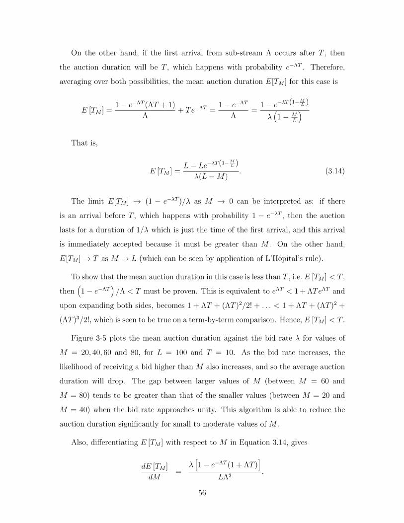
On the other hand, if the first arrival from sub-stream Λ occurs after T , then

the auction duration will be T , which happens with probability e−ΛT . Therefore,

averaging over both possibilities, the mean auction duration E[TM ] for this case is

E [TM ] =1− e−ΛT (ΛT + 1)

Λ+ Te−ΛT =

1− e−ΛT

Λ=

1− e−λT(1−ML )

λ(1− M

L

)

That is,

E [TM ] =L− Le−λT(1−M

L )

λ(L−M). (3.14)

The limit E[TM ] → (1 − e−λT )/λ as M → 0 can be interpreted as: if there

is an arrival before T , which happens with probability 1 − e−λT , then the auction

lasts for a duration of 1/λ which is just the time of the first arrival, and this arrival

is immediately accepted because it must be greater than M . On the other hand,

E[TM ]→ T as M → L (which can be seen by application of L’Hopital’s rule).

To show that the mean auction duration in this case is less than T , i.e. E [TM ] < T ,

then(1− e−ΛT

)/Λ < T must be proven. This is equivalent to eΛT < 1 + ΛTeΛT and

upon expanding both sides, becomes 1 + ΛT + (ΛT )2/2! + . . . < 1 + ΛT + (ΛT )2 +

(ΛT )3/2!, which is seen to be true on a term-by-term comparison. Hence, E [TM ] < T .

Figure 3-5 plots the mean auction duration against the bid rate λ for values of

M = 20, 40, 60 and 80, for L = 100 and T = 10. As the bid rate increases, the

likelihood of receiving a bid higher than M also increases, and so the average auction

duration will drop. The gap between larger values of M (between M = 60 and

M = 80) tends to be greater than that of the smaller values (between M = 20 and

M = 40) when the bid rate approaches unity. This algorithm is able to reduce the

auction duration significantly for small to moderate values of M .

Also, differentiating E [TM ] with respect to M in Equation 3.14, gives

dE [TM ]

dM=

λ[1− e−ΛT (1 + ΛT )

]LΛ2

.

56

0 1 2

2

4

6

8

Bid Rate

Duration

M = 20.0M = 40.0M = 60.0M = 80.0

Figure 3-5: Average auction duration of fixed-time first-price forward auction withmaximum threshold termination.

Since (1 + ΛT )/eΛT < 1, through using the expansion as in Equation 3.5, the

numerator of the above is positive, showing that

dE [TM ]

dM=

λ[1− e−ΛT (1 + ΛT )

]LΛ2

> 0.

Thus, increasing M will increase the duration of the auction. The auction income,

on the other hand, given that the auction terminates before T , can be shown to

be uniformly distributed over the interval (M,L). Since the auction income must

be greater than or equal to M , the auction income is a sample from the following

conditional density over the interval [M,L),

f(x|x ≥M) =

1

(L−M)for M ≤ x ≤ L,

0 elsewhere,

where (L−M)/L is the probability that the bid falls in the interval [M,L), and

the mean of this density is M + (L −M)/2 = (M + L)/2. Thus, the mean income

given the auction terminates before T is (M +L)/2, which happens with probability

1 − e−ΛT . There is, however, also a chance that none of the arriving bids attain the

maximum M , which happens with probability e−ΛT , and this then accepts the bid

57

with average value MN/(N + 1), with N coming from the stream Λ′. Here, L is

replaced by M since none of the associated bids are allowed to exceed M . Therefore,

the average magnitude of the accepted bid E [QM ] operating under the given auction

termination rule, from Equation 3.3, is

E [QM ] =(M + L)(1− e−ΛT )

2+Me−ΛT

Λ′T

(Λ′T + e−Λ′T − 1

), (3.15)

which is plotted in Figure 3-6, for M = 20, 40, 60 and 80, with L = 100 and

T = 10.

0 1 2

20

40

60

80

Bid Rate

Income

M = 20.0

M = 40.0

M = 60.0

M = 80.0

Figure 3-6: Average auction income of fixed-time first-price forward auction withmaximum threshold termination.

While the differences in auction income for different M values are about the same

for high bid rates, these differences tend to decline for high values of M when the

bid rate is low. When M → L; Λ → 0; Λ′ → λ then E [QM ] → LλT

(λT + e−λT − 1

),

which is in agreement with the auction income in the non-threshold termination case.

In the Open Buy-It-Now (OBIN) situation, the threshold maximum M is made

known to the bidders. While a bidder may be willing to pay an amount higher than

M , he/she does not need to do so, as paying M is sufficient to secure the good. Hence,

the above average auction income is reduced to, on replacing (M +L)/2 by M in the

58

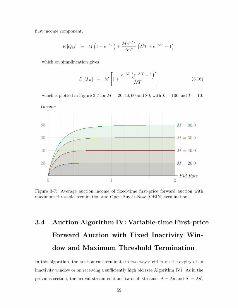
first income component,

E [QM ] = M(1− e−ΛT

)+Me−ΛT

Λ′T

(Λ′T + e−Λ′T − 1

).

which on simplification gives

E [QM ] = M

1 +e−ΛT

(e−Λ′T − 1

)Λ′T

, (3.16)

which is plotted in Figure 3-7 for M = 20, 40, 60 and 80, with L = 100 and T = 10.

0 1 2

20

40

60

80

Bid Rate

Income

M = 20.0

M = 40.0

M = 60.0

M = 80.0

Figure 3-7: Average auction income of fixed-time first-price forward auction withmaximum threshold termination and Open Buy-It-Now (OBIN) termination.

3.4 Auction Algorithm IV: Variable-time First-price


dow and Maximum Threshold Termination

In this algorithm, the auction can terminate in two ways: either on the expiry of an

inactivity window or on receiving a sufficiently high bid (see Algorithm IV). As in the

previous section, the arrival stream contains two sub-streams: Λ = λp and Λ′ = λp′,

59

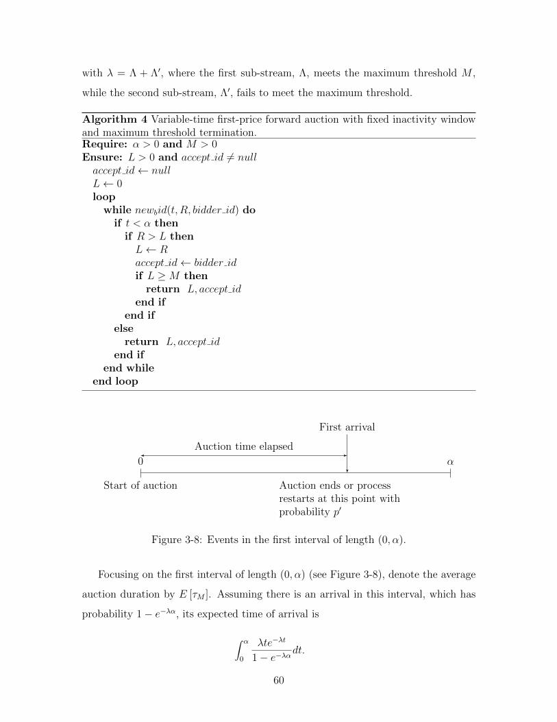
with λ = Λ + Λ′, where the first sub-stream, Λ, meets the maximum threshold M ,

while the second sub-stream, Λ′, fails to meet the maximum threshold.

Algorithm 4 Variable-time first-price forward auction with fixed inactivity windowand maximum threshold termination.Require: α > 0 and M > 0Ensure: L > 0 and accept id 6= nullaccept id← nullL← 0loop


if R > L thenL← Raccept id← bidder idif L ≥M then


end ifelse


end whileend loop

Start of auction

0

First arrival

Auction ends or processrestarts at this point withprobability p′

α

Auction time elapsed

Figure 3-8: Events in the first interval of length (0, α).

Focusing on the first interval of length (0, α) (see Figure 3-8), denote the average

auction duration by E [τM ]. Assuming there is an arrival in this interval, which has

probability 1− e−λα, its expected time of arrival is

∫ α

0

λte−λt

1− e−λαdt.

60

The denominator 1 − e−λα is present since it is given that an arrival takes place

within (0, α), and so the conditional density,

g(t|t < α) =

λe−λt

1−e−λα for 0 < t < α,

0 for t ≥ α,

is used, and this conditional average is given by

∫ α

0tg(t|t < α)dt =

1− e−λα(λα + 1)

λ (1− e−λα).

Consider this first arrival: if it comes from the Λ stream, then the auction termi-

nates immediately and no further auction time is incurred. If it comes from the Λ′

stream, however, which happens with probability p′, then further auction time will be

incurred and the process effectively restarts. That is, the additional average auction

time incurred will be p′E [τM ]. Thus, given there is an arrival in (0, α), the expected

auction duration is

1− e−λα(λα + 1)

λ (1− e−λα)+ p′E [τM ] ,

where the first term corresponds to the auction time incurred, irrespective of whether

it is an arrival from the Λ stream or an arrival from the Λ′ stream. Next, if there is no

arrival in this interval, then the auction duration is simply α (i.e. an empty auction),

which happens with probability e−λα.

Thus, averaging over the two possibilities of

1. having an arrival in the first interval of length (0, α), and

2. having no arrival in that interval,

it can be determined that

E [τM ] =(1− eλα

)1− e−λα(λα + 1)

λ (1− e−λα)+ p′E [τM ]

+ αe−λα.

61

Solving for E [τM ] yields

E [τM ] =1− e−λα

λ [p+ p′e−λα], (3.17)

which is plotted in Figure 3-9 for M = 20, 40, 60 and 80, with L = 100 and α = 3.

0 1 2

1

2

3

4

Bid Rate

Duration

M = 20.0

M = 40.0M = 60.0

M = 80.0

Figure 3-9: Average auction duration of variable-time first-price forward auction withfixed inactivity window and maximum threshold termination.

Note that as M → L, p′ → 1,

E [τM ] → 1− e−λα

λe−λα=eλα − 1

λ,

which is in agreement with Equation 3.7.

To show that E [τM ] < τα, Equation 3.17 is multiplied by eλα both in the numer-

ator and in the denominator, yielding

E [τM ] =eλα − 1

λ (p′ + peλα).

Since eλα > 1 (see Equation 3.5),

p′ + peλα > p′ + p = 1.

62

Thus,

E [τM ] =eλα − 1

λ (p′ + peλα)<eλα − 1

λ,

giving E [τM ] < τα.

As for the average auction income, consider the final interval of length, (0, α). For

the auction to terminate, there are the two possibilities of

1. no bid arrival in this interval, which occurs with probability p1 = e−λα, and

2. a bid arrival in this interval of a magnitude that falls between M and L, and

that this bid is the first bid to arrive in this interval—if this bid is not the

first bid to arrive, then this is no longer the final interval (let p2 denote the

probability of occurrence of this second possibility).

Focusing on the second possibility, let the inter-arrival time of the first sub-stream,

Λ, which meets the maximum threshold and whose arrival will terminate the auction

immediately, be X ∼ Λe−Λt, and the inter-arrival time of the second sub-stream, Λ′,

which fails to meet the maximum threshold and will allow the auction to continue,

be Y ∼ Λ′e−Λ′t. Thus, the probability p2 that the second probability occurs is:

p2 = Pr[X < α]× Pr[X < Y < α] + Pr[Y ≥ α] ,

where Pr[X < α] is the probability that a Λ-stream arrival occurs in the interval,

Pr[X < Y < α] is the probability that there is a Λ′-stream arrival also in the interval

but it occurs after the Λ′-stream arrival, and Pr[Y ≥ α] is the probability that there

is no Λ’-stream arrival in the interval. That is,

p2 =(1− e−Λα

) (Pr[X < Y < α] + e−Λ′α

).

With reference to Figure 3-10, to evaluate Pr[X < Y < α], let t ∈ (0, α) be

the arrival time of the Λ-stream, then the probability of this is Λe−Λtdt. Next, the

63

probability of arrival of the Λ′-stream in the interval (t, α) is given by

∫ α

tΛ′e−Λ′tdt = e−Λ′t − e−Λ′α.

0

First arrival of Λ-stream

t

First arrival of Λ′-stream

α

Figure 3-10: Events in the final interval of length (0, α).

Averaging over all t ∈ (0, α),

Pr[X < Y < α] =∫ α

0Λe−Λt

(e−Λ′t − e−Λ′α

)dt

=∫ α

0Λe−(Λ+Λ′)tdt−

∫ α

0Λe−Λt

(e−Λ′α

)dt

=[ −Λ

Λ + Λ′e−(Λ+Λ′)t

]α0

+ e−Λ′α[e−Λt

]α0

=Λ

Λ + Λ′

(1− e−(Λ+Λ′)α

)+ e−Λ′α

(e−Λα − 1

)=

Λ

Λ + Λ′

(1− e−(Λ+Λ′)α

)+(e−(Λ+Λ′)α − e−Λ′α

)=

(1− M

L+M

Le−λα

)− e−Λ′α.

Upon simplification, the probability of occurrence of the second possibility p2 is

p2 =(1− e−Λα

) (1− M

L+M

Le−λα

).

Therefore, the auction income using Equation 3.11 replacing L by M and λ by

Λ′, and conditioning on these two possibilities becomes

E [Q′M ] =p1

[M(1− Λ′α

eΛ′α−1

)]+ p2

(M+L

2

)p1 + p2

=e−λα

[M(1− Λ′α

eΛ′α−1

)]+(1− e−Λα

) (1− M

L+ M

Le−λα

) (M+L

2

)e−λα + (1− e−Λα)

(1− M

L+ M

Le−λα

) ,(3.18)

64


0 1 2

20

40

60

80

Bid Rate

Income

M = 20.0

M = 40.0

M = 60.0

M = 80.0

Figure 3-11: Average auction income of variable-time first-price forward auction withfixed inactivity window and maximum threshold termination.

Note that as M → L; Λ→ 0; Λ′ → λ,

E [Q′M ] → L

eλα − 1

(eλα − λα− 1

),

which is in agreement with Equation 3.11. The corresponding Open Buy-It-Now

income is

E [Q′M ] =e−λα

[M(1− Λ′α

eΛ′α−1

)]+M

(1− e−Λα

) (1− M

L+ M

Le−λα

)e−λα + (1− e−Λα)

(1− M

L+ M

Le−λα

) , (3.19)


65

0 1 2

20

40

60

80

Bid Rate

Income

M = 20.0

M = 40.0

M = 60.0

M = 80.0

Figure 3-12: Average auction income of variable-time first-price forward auction withfixed inactivity window and maximum threshold termination and Open Buy-It-Now(OBIN) termination.

3.5 Auction Algorithm V: Variable-time First-price

Forward Auction with Bid Enumeration Ter-

mination

In Algorithm I, it was mentioned that for effective auction operation, the condition,

that T 1/λ, should be met in order to ensure that there are enough bids in the

auction. Despite this, sometimes empty auctions can occur, where there are no bid

arrivals, and which can somewhat defeat the purpose of the auctioning mechanism.

For example, for Algorithm I, having no bid arrival in (0, T ) can occur with probability

e−λT , and for Algorithm II, the auction can close having no bid arrival with probability

e−λα. Thus, auction time is expended without achieving any income.

An algorithm that overcomes this empty auction problem is to terminate an auc-

tion only after a specified number of bids are received. If B is the required number of

bid arrivals, then the auction will terminate on the arrival of the B-th bid, and the

highest bid is chosen (see Algorithm V).

The average magnitude of the accepted bid, from results of order statistics (Barry

66

Algorithm 5 First-price forward auction with bid enumeration termination.

Require: B > 0Ensure: L > 0 and accept id 6= nullaccept id← nullL← 0while B > 0 do

while newbid(t, R, bidder id) doB ← B − 1if R > L thenL← Raccept id← bidder id

end ifend while


C. Arnold et al., 2008), is

E[Q(B)] =BL

B + 1, (3.20)

and is plotted in Figure 3-13 for B = 5, 10 and 15. Here, the bid rate does not

directly determine the auction income, but it has a direct impact on the duration of

the auction.

0 1 2

84

88

92

96

Bid Rate

Income

B = 5.0

B = 10.0

B = 15.0

Figure 3-13: Average auction income of variable-time first-price forward auction withbid enumeration termination.

67

The average auction duration in this case is simply the sum of B average inter-

arrival times, or B/λ, and is plotted in Figure 3-14 for B = 5, 10 and 15.

0 1 2

20

40

60

80

Bid Rate

Duration

B = 5.0B = 10.0B = 15.0

Figure 3-14: Average auction duration of variable-time first-price forward auctionwith bid enumeration termination.

Looking at duration, it is interesting to compare the average auction duration of

Algorithm V with those of Algorithms 1 and 2. If B/λ < T or B < λT , then the

average auction duration of Algorithm V will be shorter than that of Algorithm I.

For the average duration of Algorithm 5 to be shorter than that of Algorithm II, the

following condition must be fulfilled:

eλα − 1 > B,

giving

α >loge(1 +B)

λ.

For example, for B = 8 and λ = 0.5, for the average auction duration of Algo-

rithm V to be longer than that of Algorithm V, α must be larger than 4.4.

Looking at income, the average auction income of AAlgorithm V is an increasing

68

function of B because

dE[Q(B)

]dB

=L

(B + 1)2> 0.

For the average auction income of Algorithm V to be less than that of Algorithm I,

the following condition must be fulfilled:

BL

B + 1<

L

λT

(λT + e−λT − 1

),

giving

B <λT

1− e−λT− 1.

Similarly, for the average auction income of Algorithm V to be less than that of

Algorithm II, the following condition must be fulfilled:

BL

B + 1<

L

eλα − 1

(eλα − λα− 1

),

giving

B <eλα − 1

λα− 1.

3.6 Results Summary

This chapter has studied the properties of five Internet auction algorithms exhibiting

different characteristics. Closed-form expressions are obtained for the average auction

duration, and average auction income, which are the key measures of Internet auction

performance. These results are summarised in Table 3.1.

For the fixed-time first-price forward auction, as expected, an increase in the

number of bids results in a corresponding increase in average auction income. The

size of the average bid rate is a strong determinant of the amount of income obtained

69

in the auction and an increase in bid rate up to a certain point produces a rather

marked increase in auction income rate, though there seems to be a critical bid rate

above which the increase in auction income rate slows down.

For the variable-time first-price forward auction with fixed inactivity window, the

inactivity window, α, should not be significantly smaller than the mean bid inter-

arrival time, otherwise the auction will end without any or many bids. In the same

way, if it is much larger than the mean bid inter-arrival time, the auction may drag

on indefinitely with minimum impact on the income obtained in the auction.

For the fixed-time first-price forward auction with maximum threshold termina-

tion, similar to the Buy-It-Now (BIN) option in eBay, the threshold, M , needs to be

set carefully. Setting M much higher than average auction income will mean that

early termination of the auction before T is unlikely, while setting M to be very

small would mean that the first bid is likely to be accepted, which is the same as not

conducting an auction at all.

For the variable-time first-price forward auction with fixed inactivity window and

maximum threshold termination, varying the bid rate makes for very interesting re-

sults. As the bid rate increases, there is an interplay of two forces that affect the

duration of the auction: the auction duration lengthens as a result of an increased

probability that a bid arrives in the α interval; the auction duration shortens as the

probability of a bid hitting the maximum threshold is increased. This interplay can

be seen in Figure 3-9.

70

Algorithm Average Auction Duration Average Offer Accepted Per Auction

I T LλT

(λT + e−λT − 1

)

II eλα−1λ

Leλα−1


]

III

L−Le−λT(1−ML )

λ(L−M)

(M+L)(1−e−ΛT )2

+ Me−ΛT

Λ′T

(Λ′T + e−Λ′T − 1

)[CBIN]


λ(L−M)M(1− e−ΛT

)+ Me−ΛT

Λ′T

(Λ′T + e−Λ′T − 1

)[OBIN]

IV

1−e−λαλ[p+p′e−λα]

e−λα[M

(1− Λ′α

eΛ′α−1

)]+(1−e−Λα)(1−M

L+MLe−λα)(M+L

2 )

e−λα+(1−e−Λα)(1−ML

+MLe−λα)

[CBIN]

1−e−λαλ[p+p′e−λα]

e−λα[M

(1− Λ′α

eΛ′α−1

)]+M(1−e−Λα)(1−M

L+MLe−λα)

e−λα+(1−e−Λα)(1−ML

+MLe−λα)

[OBIN]

V Bλ

BLB+1

Table 3.1: First-price forward auctions.

71

Chapter 4

Analysis of Vickrey and Reverse

Auction Algorithms

The previous chapter studied Internet auction algorithms which were first-price for-

ward auctions. As Internet auctions can take on a variety of forms, this chapter

studies other Internet auction algorithms which are prevalent on the Internet. There

are two main classes of algorithms: the first is related to Vickrey auctions, and the

second is related to reverse auctions.

Vickrey auctions are commonly used for the reason that it gives bidders an in-

centive to bid an item’s true value without needing to worry about overpaying. For

markets where liquidity is an issue, Vickrey auctions can be dangerous. An example

of this is demonstrated in a New Zealand spectrum auction, where there were only

to participants. While the first bid ran into the hundreds of thousands of dollars, the

second bid was a token bid in the tens of dollars. As this was a Vickrey auction, the

winner received a discount of four orders of magnitude, a far cry from the true value

that the buyer was willing to pay.

Reverse auctions are used for for obtaining low prices. This is often used when

supply outstrips demand. It is frequently used in procurement where a government or

private sector organisation wishes to obtain goods or services and the sellers compete

against each other in providing the goods or services at increasingly lower prices.

Note that this is different from a Dutch auction, which some also consider to be a

73

reverse auction. In a Dutch auction, the auction still seeks to obtain as high a price

as possible and involves an auctioneer starting at a very high asking price that is

continually lowered until some bidder is willing to accept the offer. The advantage

of this is that auctions can happen very fast as it only takes a single bid to end the

auction; it plays off bidders’ fear of losing out and their drive towards a lower price.

4.1 Auction Algorithm VI: Fixed-time Vickrey For-

ward Auction

Various forms of Vickrey auctions, which can also be called second-price auctions, are

commonly found on the Internet. In eBay ’s system of proxy bidding, for example,

the auction winner does not pay the highest bid, but the value of the second-highest

bid plus a bid increment. Variations exist for the increment charged by the auction

mechanism which may be a fixed increment, or one that depends on the value of

the relevant bid. An advantage of Vickrey auctions is that it gives bidders an incen-

tive to bid an item’s true value without needing to worry about overpaying. As in

Algorithm I, the auction time here is fixed with duration T . For effective auction op-

eration, one would need to have at least two bids, and thus T should be significantly

greater than twice the mean inter-arrival time 1/λ. If N is the number of bid arrivals

in the time interval (0, T ), then at the close of the auction, the auctioning mechanism

will pick the bidder of maximum bid Q(N) to be the winner while the amount the

winner pays will be Q(N−1) (see Algorithm VI).

From the results of order statistics (Barry C. Arnold et al., 2008), it can be shown

that the conditional income per auction, or the second-largest order statistic, is

E[Q(N−1)|Number of bids = N ] =(N − 1)L

N + 1(4.1)

To remove the condition on N , three cases are considered:

1. N = 0. Here the income is zero.

74

Algorithm 6 Fixed-time Vickrey forward auction.

Require: δ > 0 and T > 0Ensure: L2 + δ > 0 and accept id1 6= nullaccept id1← nullaccept id2← nullclock ← 0L1← 0L2← 0while clock < T do

while newbid(t, R, bidder id) doclock ← clock + tif clock < T then

if R > L1 thenL2← L1L1← Raccept id2← accept id1accept id1← bidder id

else if R > L2 thenL2← Raccept id2← bidder id

end ifend if

end whileend whilereturn L2 + δ, accept id1

75

2. N = 1. Here the income is zero plus an appropriate bid increment δo.

3. N ≥ 2. Here the Vickrey auction functions normally, and a bid increment δ

will apply.

Disregarding the bid increments temporarily, since Equation 4.1 gives zero for

N = 1, cases (ii) and (iii) can be combined and the equation can be summed from

N = 1, i.e.

E[Q(N−1)

]=

∞∑N=1

(N − 1)L

N + 1× e−λT (λT )N

N !

=∞∑N=1

[L− 2L

N + 1

]× e−λT (λT )N

N !

=∞∑N=1

L× e−λT (λT )N

N !−∞∑N=1

2L

N + 1× e−λT (λT )N

N !.

Using the same technique as Equation 3.2,

E[Q(N−1)

]= L

(1− e−λT

)− 2Le−λT

λT

(eλT − 1− λT

)=

L

λT

(λT + λTe−λT + 2e−λT − 2

). (4.2)

Thus, incorporating the bid increments of the last two cases above, results in an

income of

λTe−λT δo +L

λT


)+ δ, (4.3)

where the first term corresponds to the case N = 1. This is plotted in Figure 4-1, for

T = 5, 10 and 15, with L = 100 and δo = δ = 0.

It is useful to compare the average auction incomes of Algorithms 1 and 6. The

difference between the two average auction incomes is

E [∆1Q] = E[Q(N) −Q(N−1)

]=

L

λT

(λT + e−λT − 1

)− L

λT


).

76

0 2 4 6 8 10

60

70

80

90

Bid Rate

Income

T = 5.0T = 10.0T = 15.0

Figure 4-1: Average auction income of fixed-time Vickrey forward auction.

Simplifying gives

E [∆1Q] =L

λT

[1− e−λT (1 + λT )

]. (4.4)

Since (1 + λT )/eλT < 1, which can be seen on expanding eλT for λT > 0, it can

be seen that E [∆1Q] is always greater than zero. As the average number of bids

becomes very small, however, on application of L’Hopital’s rule on Equation 4.4, it

can be seen that

E [∆1Q]→ 0 as λT → 0

On the other hand, it is also interesting to see that as the average number of bids

becomes very large, the same limit is approached.

E [∆1Q]→ 0 as λT →∞

To see this, Equation 4.4 can be rewritten as

E [∆1Q] = L

[1

λT− e−λT

λT− e−λT

]. (4.5)

77

Thus, as λT →∞, the above approaches zero. The reason for this is that, as the

average number of bids becomes very large, the average auction income in both cases

will approach the same limit L such that there is very little difference between them,

i.e.

E[Q(N)

]=

L

λT

(λT + e−λT − 1

)→ L as λT →∞

E[Q(N−1)

]=

L

λT


)→ L as λT →∞

A comparison of E[Q(N)

]and E

[Q(N−1)

]is plotted in Figure 4-2, for T = 10,

with L = 100, T = 10 and δ0 = δ = 0. The difference between the two is significant

for low bid rates but narrows as the bid rate increases.

0 2 4 6 8 10

60

70

80

90

Bid Rate

Income

E[Q(N)

]E[Q(N−1)

]

Figure 4-2: Average auction income comparison between the fixed-time first-priceforward auction and the fixed-time Vickrey forward auction.

78

4.2 Auction Algorithm VII: Variable-time Vickrey


dow

Here, like Algorithm II, the auction will terminate when there is no bid arrival for

a fixed window of length α. On termination, the second-largest bid received will be

accepted (see Algorithm VII).

Algorithm 7 Variable-time Vickrey forward auction with fixed inactivity window.

Require: α > 0 and δ > 0Ensure: L2 + δ > 0 and accept id1 6= nullaccept id1← nullaccept id2← nullL1← 0L2← 0loop


if R > L1 thenL2← L1L1← Raccept id2← accept id1accept id1← bidder id


end ifelse

return L2 + δ, accept id1end if

end whileend loop

Ignoring the bid increments temporarily, the condition on N in Equation 4.1 is

removed in order to determine the average income E[Q(N−1)

]. As in Algorithm II,

the following probabilities are used:

Pr[T1 < α, T2 < α, . . . , TN < α, TN+1 ≥ α] =(1− e−λα

)N× e−λα

79

Summing from N = 1 as in the previous algorithm,

E[Q(N−1)

]=

∞∑N=1

(N − 1)L

N + 1× (1− e−λα)Ne−λα

=∞∑N=1

[L− 2L

N + 1

]×(1− e−λα

)Ne−λα

=∞∑N=1

L(1− e−λα

)Ne−λα − 2Le−λα

(1− e−λα)

∞∑N=1

(1− e−λα

)N+1

N + 1

= L(1− e−λα

)− 2Le−λα

(1− e−λα)

∞∑N=1

(1− e−λα

)N+1

N + 1

Using the logarithmic series given in Equation 3.10, this gives,

E[Q(N−1)

]= L

(1− e−λα

)− 2L

eλα − 1

[λα + e−λα − 1

].

On simplification and grouping terms, and on noting that (ex − e−x)/2 may be

simply written as sinh(x), we have

E[Q(N−1)

]=

2L

eλα − 1[sinhλα− λα] . (4.6)

Incorporating the bid increments, this yields an expected auction income of

(1− e−λα

)× e−λαδo +

2L

eλα − 1[sinhλα− λα] + δ. (4.7)

Figure 4-3 shows the auction income for different values of λ for L = 100, α = 1, 2

and 3, δo = δ = 0. Note that the average auction income rises rather rapidly for small

values of λ, but stabilises and yields only slight improvement as the bid rate increases

beyond 2.

It is useful to compare the average auction incomes of Algorithms 2 and 7. The

difference between the two average auction incomes is

E [∆2Q] = E[Q(N) −Q(N−1)

]=

L

eλα − 1


]− 2L

eλα − 1[sinhλα− λα] .

80

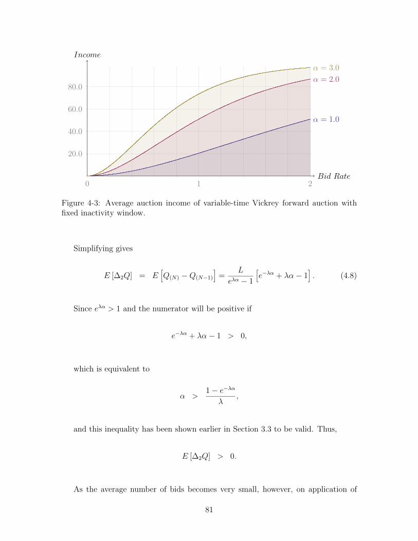
0 1 2

20.0

40.0

60.0

80.0

Bid Rate

Income

α = 1.0

α = 2.0

α = 3.0

Figure 4-3: Average auction income of variable-time Vickrey forward auction withfixed inactivity window.

Simplifying gives

E [∆2Q] = E[Q(N) −Q(N−1)

]=

L

eλα − 1

[e−λα + λα− 1

]. (4.8)

Since eλα > 1 and the numerator will be positive if

e−λα + λα− 1 > 0,

which is equivalent to

α >1− e−λα

λ,

and this inequality has been shown earlier in Section 3.3 to be valid. Thus,

E [∆2Q] > 0.

As the average number of bids becomes very small, however, on application of

81

L’Hopital’s rule on Equation 4.8, it can be seen that

E [∆2Q]→ 0.

On the other hand, as the average number of bids per window λα approaches

infinity, the first and third terms of Equation 4.8 tends toward zero. As for the

second term,

λα

eλα − 1=

λα

λα + (λα)2

2!+ (λα)3

3!+ . . .

→ 0.

Thus, as λα→∞,

E [∆2Q]→ 0.

Therefore, as the number of bids in a window becomes large, there is little differ-

ence in auction income between the first-price and the corresponding Vickrey auctions.

This is plotted in Figure 4-4, for α = 2, with L = 100, and δ0 = δ = 0.

0 1 2

20.0

40.0

60.0

80.0

Bid Rate

Income

E[Q(N)

]E[Q(N−1)

]

Figure 4-4: Average auction income comparison between the variable-time first-priceforward auction with fixed inactivity window and the variable-time Vickrey forwardauction with fixed inactivity window.

The auction duration for Algorithm VII is the same as that of Algorithm II and

82

is given by Equation 3.7.

4.3 Auction Algorithm VIII: Fixed-time Vickrey

Forward Auction with Maximum Threshold

Termination

This is similar to Algorithm III, except that if the auction continues through to

completion, the accepted bid will be the second highest bid (see Algorithm VIII).

Algorithm 8 Fixed-time Vickrey forward auction with maximum threshold termi-nation.Require: δ > 0 and M > 0 and T > 0Ensure: L2 + δ > 0 and accept id1 6= nullaccept id1← nullaccept id2← nullclock ← 0L1← 0L2← 0while clock < T do

while newbid(t, R, bidder id) doclock ← clock + tif clock < T then

if R > L1 thenL2← L1L1← Raccept id2← accept id1accept id1← bidder idif L1 ≥M then

return L1, accept id1end if


end ifend if

end whileend whilereturn L2 + δ, accept id1

The average auction duration here is the same as Algorithm III, and is given

83

by Equation 3.14. The mean bid accepted given the auction terminates before T is

M+L2

, which happens with probability(1− e−ΛT

). If none of the arriving bids attain

the maximum M , which happens with probability e−ΛT , the bid with average value

L(N − 1)/(N + 1) is accepted, with N here coming from the stream Λ′. Here, L is

replaced by M since none of the associated bids are allowed to exceed M . Therefore,

the average magnitude of the accepted bid E[QMv] operating under the given auction

termination rule, from Equation 4.2, is

E[QMv] =(M + L)

(1− e−ΛT

)2

+Me−ΛT

Λ′T

(Λ′T + Λ′Te−Λ′T + 2e−Λ′T − 2

), (4.9)

which is plotted in Figure 4-5, for M = 20, 40, 60 and 80, with L = 100, T = 10

and δ0 = δ = 0.

0 1 2

20.0

40.0

60.0

80.0

Bid Rate

Income

M = 20.0

M = 40.0

M = 60.0

M = 80.0

Figure 4-5: Average auction income of fixed-time Vickrey forward auction with max-imum threshold termination.

The corresponding Open Buy-It-Now (OBIN) income is, on replacing (M + L)/2

by M in the first term,

E[QMv] = M(1− e−ΛT

)+Me−ΛT

Λ′T

(Λ′T + Λ′Te−Λ′T + 2e−Λ′T − 2

), (4.10)

which is plotted in Figure 4-6, for M = 20, 40, 60 and 80, with L = 100 and

84

T = 10.

It is interesting to note that the curves on this graph cross-over. The reason for

this is that, for small M , the income is likely to be (M + L)/2 which basically is like

the first-price auction, while for large M , no bid exceeds M and hence the second

price would have to be accepted. Thus, the income drops from (M + L)/2 to second

price. Similar reasoning also applies to Figures 4-5, 4-6 and 4-8.

0 1 2

20.0

40.0

60.0

80.0

Bid Rate

Income

M = 20.0

M = 40.0

M = 60.0

M = 80.0

Figure 4-6: Average auction income of fixed-time Vickrey forward auction with max-imum threshold termination and Open Buy-It-Now (OBIN) termination.

The auction duration for Algorithm VIII is the same as that of Algorithm III and


4.4 Auction Algorithm IX: Variable-time Vickrey


dow and Maximum Threshold Termination

This algorithm is similar to Algorithm IV, except that if the auction continues through

to normal completion, the accepted bid will be the second-highest bid (see Algo-

rithm IX).

85

Algorithm 9 Variable-time Vickrey forward auction with fixed inactivity windowand maximum threshold termination.Require: α > 0 and δ > 0 and M > 0Ensure: L2 + δ > 0 and accept id1 6= nullaccept id1← nullaccept id2← nullL1← 0L2← 0loop


if R > L1 thenL2← L1L1← Raccept id2← accept id1accept id1← bidder idif L1 ≥M then

return L1, accept id1end if


end ifelse

return L2 + δ, accept id1end if

end whileend loop

86

As per the derivation for Algorithm IV, the mean accepted bid E[Q′Mv], averaging

over both termination possibilities, from Equation 4.6, is

E [Q′Mv] =e−λα 2M

exp(Λ′α)−1[sinh(Λ′α)− Λ′α] +

(1− e−Λα

) (1− M

L+ M

Le−λα

) (M+L

2

)e−λα + (1− e−Λα)

(1− M

L+ M

Le−λα

) ,(4.11)

which is plotted in Figure 4-7, for M = 20, 40, 60 and 80, with L = 100, α = 3

and δ0 = δ = 0.

0 1 2

20.0

40.0

60.0

80.0

Bid Rate

Income

M = 20.0

M = 40.0

M = 60.0

M = 80.0

Figure 4-7: Average auction income of variable-time Vickrey forward auction withfixed inactivity window and maximum threshold termination.

In the Open Buy-It-Now (OBIN) situation, where M is made known to the bid-

ders, the average auction income is, from Equation 4.11 on replacing (M + L)/2 by

M in the second term,

E [Q′Mv] =e−λα 2M

exp(Λ′α)−1[sinh(Λ′α)− Λ′α] +M

(1− e−Λα

) (1− M

L+ M

Le−λα

)e−λα + (1− e−Λα)

(1− M

L+ M

Le−λα

) ,(4.12)

which is plotted in Figure 4-8, for M = 20, 40, 60 and 80, with L = 100, T = 10

and δ0 = δ = 0.

The auction duration for Algorithm IX is the same as that of Algorithm IV and


87

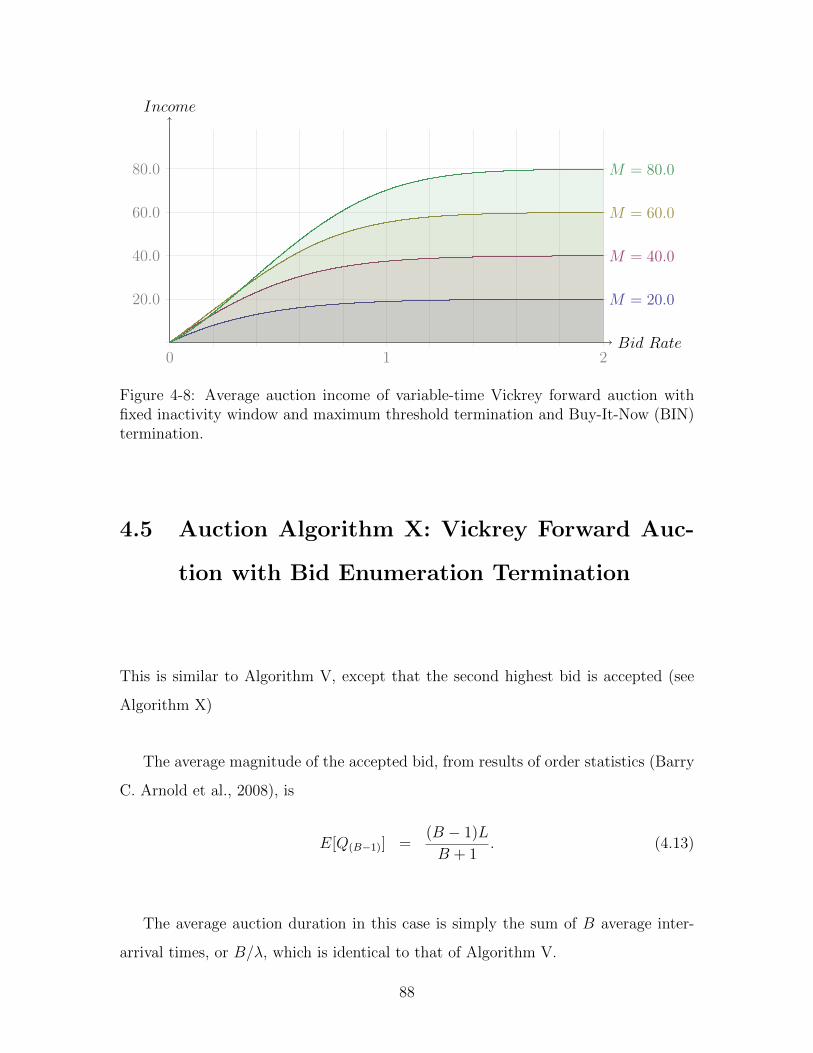
0 1 2

20.0

40.0

60.0

80.0

Bid Rate

Income

M = 20.0

M = 40.0

M = 60.0

M = 80.0

Figure 4-8: Average auction income of variable-time Vickrey forward auction withfixed inactivity window and maximum threshold termination and Buy-It-Now (BIN)termination.

4.5 Auction Algorithm X: Vickrey Forward Auc-

tion with Bid Enumeration Termination

This is similar to Algorithm V, except that the second highest bid is accepted (see

Algorithm X)

The average magnitude of the accepted bid, from results of order statistics (Barry

C. Arnold et al., 2008), is

E[Q(B−1)] =(B − 1)L

B + 1. (4.13)

The average auction duration in this case is simply the sum of B average inter-

arrival times, or B/λ, which is identical to that of Algorithm V.

88

Algorithm 10 Vickrey forward auction with bid enumeration termination.

Require: B > 0Ensure: L2 + δ > 0 and accept id1 6= nullaccept id1← nullaccept id2← nullL1← 0L2← 0while B > 0 do

while newbid(t, R, bidder id) doB ← B − 1if R > L1 thenL2← L1L1← Raccept id2← accept id1accept id1← bidder id


end ifend while

end whilereturn L2 + δ, accept id1

4.6 Auction Algorithm XI: Fixed-time Last-price

Reverse Auction

Some Internet auction processes follow the reverse auction mechanism. It is also fre-

quently used in e-procurement where governments and private sectors wish to obtain

goods or services (e.g. http://www.esourcingsolutions.co.uk). Typically, buyers

indicate what they require, with the sellers competing against each other to provide

the goods or services, and in doing so, the price is driven down. At the close of the

reverse auction, the lowest bid is selected (see Algorithm XI).

Note that this is different from a Dutch auction, which some also consider to be a

reverse auction. In a Dutch auction, the auction still seeks to obtain as high a price

as possible and involves an auctioneer starting at a very high asking price that is

continually lowered until some bidder is willing to accept the offer. The advantage

of this is that auctions can happen very fast as it only takes a single bid to end the

89

auction; it plays off bidders’ fear of losing out and their drive towards a lower price.

Algorithm 11 Fixed-time last-price reverse auction.

Require: T > 0Ensure: L > 0 and accept id 6= nullaccept id← nullclock ← 0L←∞while clock < T do

while newbid(t, R, bidder id) doclock ← clock + tif clock < T and R < L thenL← Raccept id← bidder id

end ifend while


Here, we are interested in E[Q(1)], and the aim is to minimise expenditure rather

than maximising income. Again, from (Barry C. Arnold et al., 2008), it can be shown

that

E[Q(1)|Number of bids = N ] =L

N + 1(4.14)

Unlike the forward auction situation, however, where for N = 0, the auction

income is zero, here, when N = 0, the maximum expenditure of L has to be paid,

so the term N = 0 cannot be ignored. Thus, following the techniques of previous

analysis, we have, for the unconditional average

E[Q(1)] =∞∑N=0

L

N + 1× e−λT (λT )N

N !

=Le−λT

λT

∞∑N=0

(λT )N+1

(N + 1)!

=L

λT

[1− e−λT

], (4.15)

which is plotted in Figure 4-9, for T = 5, 10 and 15, with L = 100 and δ0 = δ = 0.

90

0 2 4 6 8 10

2

4

6

8

Bid Rate

Expenditure

T = 5.0

T = 10.0T = 15.0

Figure 4-9: Average auction expenditure of fixed-time last-price reverse auction.

This gives an expenditure of

L

λT 2

[1− e−λT

]. (4.16)

4.7 Auction Algorithm XII: Variable-time Last-

price Reverse Auction with Fixed Inactivity

Window

Similar to Algorithm II, here the auction will terminate when there is no bid arrival

for a fixed window of length α. On termination, the smallest bid received will be

chosen (see Algorithm XII).

Here, the average auction duration is the same as that of Algorithm II, and is given

by Equation 3.7. Following similar arguments and using the same de-conditioning

probabilities as in Section 3.2, we have, from Equation 4.14.

E[Q(1)] =∞∑N=0

L

N + 1×(1− e−λα

)Ne−λα =

Le−λα

1− e−λα∞∑N=0

(1− e−λα)N+1

N + 1(4.17)

91

Algorithm 12 Variable-time last-price reverse auction with fixed inactivity window.

Require: α > 0Ensure: L > 0 and accept id 6= nullaccept id← nullL←∞loop


if R < L thenL← Raccept id← bidder id

end ifelse


end whileend loop

This gives, on making use of the logarithmic series in Equation 3.10,

E[Q(1)] =Lλα

eλα − 1, (4.18)

which is plotted in Figure 4-10, for α = 1, 2 and 3, with L = 100 and δ0 = δ = 0.

0 1 2

20.0

40.0

60.0

80.0

Bid Rate

Expenditure

α = 1.0

α = 2.0α = 3.0

Figure 4-10: Average auction expenditure of variable-time last-price reverse auctionwith fixed inactivity window.

92

4.8 Auction Algorithm XIII: Fixed-time Last-price

Reverse Auction with Minimum Threshold Ter-

mination

This is similar to Algorithm III, except that the auction may terminate before the

expiry of T , if a sufficiently low bid is received. We let this minimum threshold be m,

so that whenever an arriving bid is below or equal to m, then the auction terminates

immediately and that bid is accepted. Thus, if a low enough bid is received, one

would not wish to waste any more time in waiting for another offer, which may or

may not result in an improvement (see Algorithm XIII)

Algorithm 13 Fixed-time last-price reverse auction with minimum threshold termi-nation.Require: M > 0 and T > 0Ensure: L > 0 and accept id 6= nullaccept id← nullclock ← 0L←∞while clock < T do

while newbid(t, R, bidder id) doclock ← clock + tif clock < T and R < L thenL← Raccept id← bidder idif L ≤M then


end ifend while


Analogous to the Buy-It-Now (BIN) situation in forward auctions, in the Sell-It-

Now (SIN) situation, if a bid arrives with a value that is less than or equal to m, it is

immediately accepted. As in the forward auctions, the value m may be kept private

or made known to the public.

Here, we let p = Pr[Bid ≤ m] = m/L, p′ = Pr[Bid > m] = 1 − m/L. Thus,

93

for each arrival, there is a probability p that it will meet the minimum threshold

requirement. There are two Poisson arrival streams with rates Λ = λp and Λ′ = λp′,

with λ = Λ+Λ′. The first sub-stream Λ meets the minimum threshold and its arrival

will terminate the auction immediately, while the second sub-stream Λ′ fails to meet

the minimum threshold and will allow the auction to continue. The first arrival of

the Λ sub-stream at time t before T would terminate the auction at t immediately,

which happens with probability Λe−Λtdt. Averaging over all such arrivals before T

gives

∫ T

0Λte−Λtdt =

1− eΛt(ΛT + 1)

Λ.

On the other hand, if the first arrival from this sub-stream Λ occurs after T , then

the auction duration would be T , which happens with probability e−ΛT . Therefore,

averaging over both possibilities, we have for the mean auction duration E[Tm] for

this case

E[Tm] =1− eΛt(ΛT + 1)

Λ+ Te−ΛT =

1− e−ΛT

Λ=

1− e−λmT/L

λm/L

That is,

E[Tm] =L− Le−λmT/L

λm. (4.19)

We see that E[Tm] →(1− e−λT

)/λ as m → L, which may be interpreted as:

if there is an arrival before T , which happens with probability(1− e−λT

), then the

auction lasts for a duration of 1/λ which is just the time of the first arrival, and this

arrival is immediately accepted because it must be less than m. On the other hand,

as m→ 0, E[Tm]→ T (which can be seen by application of L’Hopital’s rule). Again,

as shown previously in Section 3.3,(1− e−ΛT

)/Λ < T , which shows that E[Tm] < T .

Figure 4-11 plots the mean auction duration against the bid rate λ for values of

m = 25, 50, 75 for L = 100 and T = 4. We see that, as the bid rate increases, the

likelihood of receiving a bid less than m also increases, and so the average auction

94

duration drops. This algorithm is able to reduce the auction duration from T = 4 for

moderate to large values of m quite substantially.

0 1 2

2

4

6

8

Bid Rate

Duration

m = 25.0m = 50.0

m = 75.0

Figure 4-11: Average auction duration of fixed-time last-price reverse auction withminimum threshold termination.

In determining the average auction expenditure, the symmetry between the cur-

rent algorithm and Algorithm III is used. Considering the interval (0, L), and noting

that the distance or magnitude between the auction income and L in Algorithm III

is the same as that between the auction expenditure here and 0, which is precisely

the average auction expenditure in the present algorithm. Thus, the current average

auction expenditure is given by

L− E [QM ] ,

and on replacing M by L−m, the average auction expenditure can be obtained:

E [Qm] = L−

(2L−m)(1− e−ΛT

)2

+(L−m)e−ΛT

Λ′T

(Λ′T + e−Λ′T − 1

) ,(4.20)

where Λ′ = λm/L and Λ = λ(1 −m/L) and which is plotted in Figure 4-12, for

m = 20, 40, 60 and 80, with L = 100, T = 10 and δ0 = δ = 0.

95

0 1 2

20.0

40.0

60.0

80.0

Bid Rate

Expenditure

m = 20.0

m = 40.0

m = 60.0

m = 80.0

Figure 4-12: Average auction expenditure of fixed-time last-price reverse auction withminimum threshold termination and Closed Sell-It-Now (CSIN).

For the Open Sell-It-Now (OSIN) case, the average auction expenditure is

E [Qm] = L−[(L−m)

(1− e−ΛT

)+

(L−m)e−ΛT

Λ′T

(Λ′T + e−Λ′T − 1

)](4.21)

which is plotted in Figure 4-13, for m = 20, 40, 60 and 80, with L = 100, T = 10

and δ0 = δ = 0.

0 1 2

20.0

40.0

60.0

80.0

Bid Rate

Expenditure

m = 20.0

m = 40.0

m = 60.0

m = 80.0

Figure 4-13: Average auction expenditure of fixed-time last-price reverse auction withminimum threshold termination and Open Sell-It-Now (OSIN).

96

4.9 Auction Algorithm XIV: Variable-time Last-

price Reverse Auction with Fixed Inactivity

Window and Minimum Threshold Termination

This is similar to Algorithm XII with an additional termination condition that the

auction mechanism will accept a bid if it is sufficiently low (see Algorithm XIV).

Here, the auction can be terminated either

1. by having none of the bid arrivals meeting the minimum threshold and the

auction finishes on the expiry of a no bid interval of length α, or

2. by having an arrival which meets the minimum threshold m before the auction

terminates through (1).

Algorithm 14 Variable-time last-price reverse auction with fixed inactivity windowand minimum threshold termination.Require: α > 0 and M > 0Ensure: L > 0 and accept id 6= nullaccept id← nullL←∞loop


if R < L thenL← Raccept id← bidder idif L ≤M then


end ifelse


end whileend loop

As in the previous algorithm, the auction expenditure here is best determined

by observing the symmetry between the auction expenditure here and that in Algo-

97

rithm IV. Thus, the average auction expenditure here is:

L− E [Q′M ] , (4.22)

which can be written as, on replacing M by (L−m),

L−(L−m)e−λα

[1− Λ′α

eΛ′α−1

]+(1− e−Λα

) [1− (L−m

L+ L−m

Le−λα

] (2L−m

2

)e−λα + (1− e−Λα)

(1− L−m

L+ L−m

Le−λα

) , (4.23)

which is plotted in Figure 4-14, for m = 20, 40, 60 and 80, with L = 100, α = 3

and δ0 = δ = 0.

0 1 2

20.0

40.0

60.0

80.0

Bid Rate

Expenditure

m = 20.0

m = 40.0

m = 60.0

m = 80.0

Figure 4-14: Average auction expenditure of variable-time last-price reverse auctionwith fixed inactivity window and minimum threshold termination and Closed Sell-It-Now (CSIN).

For the Open Sell-It-Now (OSIN) case, the average auction expenditure is

L−(L−m)e−λα

[1− Λ′α

eΛ′α−1

]+ (L−m)

(1− e−Λα

) [1− (L−m

L+ L−m

Le−λα

]e−λα + (1− e−Λα)

(1− L−m

L+ L−m

Le−λα

) (4.24)

which is plotted in Figure 4-15, for M = 20, 40, 60 and 80, with L = 100, α = 3

and δ0 = δ = 0.

98

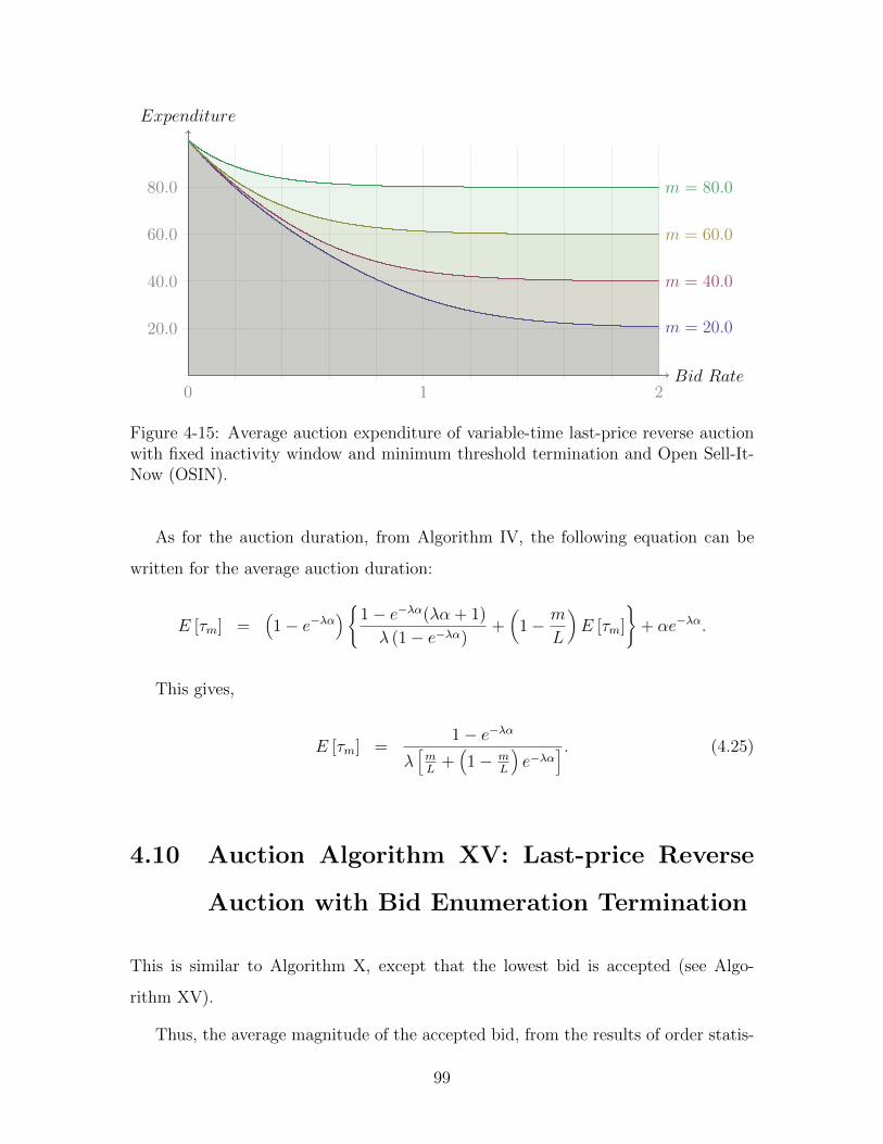
0 1 2

20.0

40.0

60.0

80.0

Bid Rate

Expenditure

m = 20.0

m = 40.0

m = 60.0

m = 80.0

Figure 4-15: Average auction expenditure of variable-time last-price reverse auctionwith fixed inactivity window and minimum threshold termination and Open Sell-It-Now (OSIN).

As for the auction duration, from Algorithm IV, the following equation can be

written for the average auction duration:

E [τm] =(1− e−λα

)1− e−λα(λα + 1)

λ (1− e−λα)+(

1− m

L

)E [τm]

+ αe−λα.

This gives,

E [τm] =1− e−λα

λ[mL

+(1− m

L

)e−λα

] . (4.25)

4.10 Auction Algorithm XV: Last-price Reverse

Auction with Bid Enumeration Termination

This is similar to Algorithm X, except that the lowest bid is accepted (see Algo-

rithm XV).

Thus, the average magnitude of the accepted bid, from the results of order statis-

99

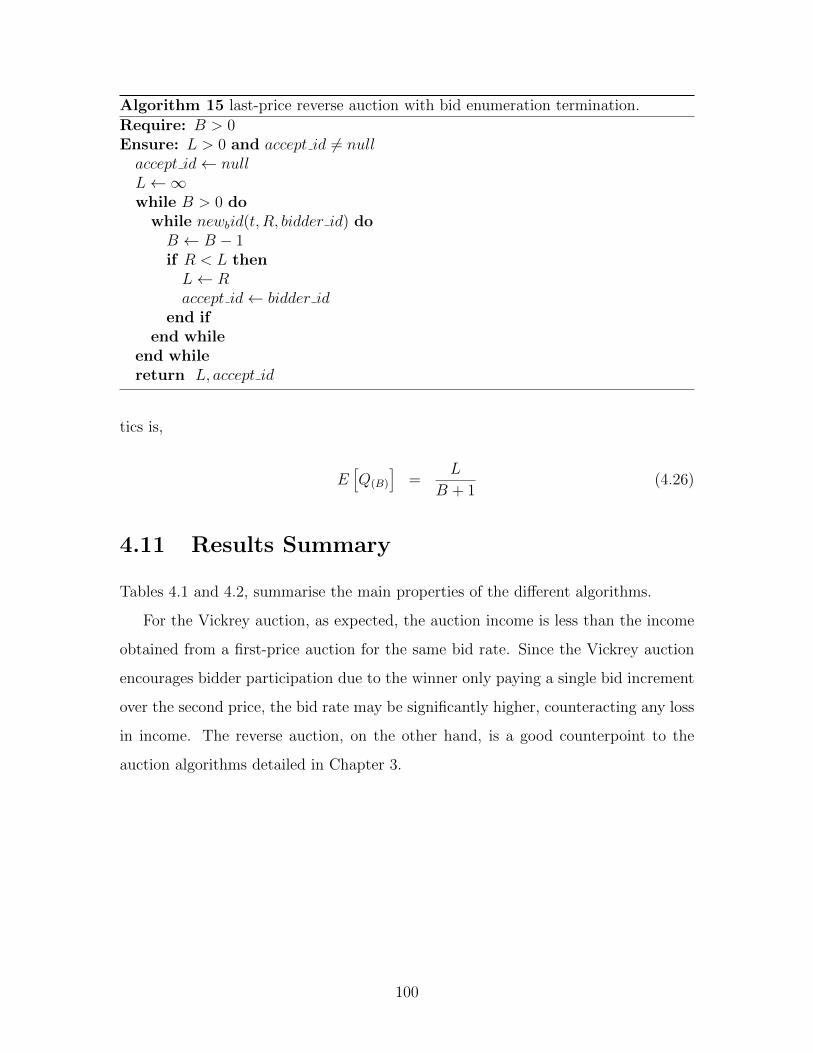
Algorithm 15 last-price reverse auction with bid enumeration termination.

Require: B > 0Ensure: L > 0 and accept id 6= nullaccept id← nullL←∞while B > 0 do

while newbid(t, R, bidder id) doB ← B − 1if R < L thenL← Raccept id← bidder id

end ifend while


tics is,

E[Q(B)

]=

L

B + 1(4.26)

4.11 Results Summary

Tables 4.1 and 4.2, summarise the main properties of the different algorithms.

For the Vickrey auction, as expected, the auction income is less than the income

obtained from a first-price auction for the same bid rate. Since the Vickrey auction

encourages bidder participation due to the winner only paying a single bid increment

over the second price, the bid rate may be significantly higher, counteracting any loss

in income. The reverse auction, on the other hand, is a good counterpoint to the

auction algorithms detailed in Chapter 3.

100


VI T λTe−λT δo + LλT


)+ δ

VII eλα−1λ

(1− e−λα

)× e−λαδo + 2L

eλα−1[sinhλα− λα] + δ

VIII


λ(L−M)

(M+L)(1−e−ΛT )2

+ Me−ΛT

Λ′T

(Λ′T + Λ′Te−Λ′T + 2e−Λ′T − 2

)[CBIN]


λ(L−M)M(1− e−ΛT

)+ Me−ΛT

Λ′T

(Λ′T + Λ′Te−Λ′T + 2e−Λ′T − 2

)[OBIN]

IX

e−Λα

[1−e−Λ′α(Λ′α+1)

]Λ′[1−e−Λα(1−e−Λ′α)]

+ 1−e−Λα

Λ

(1−e−Λα)(M+L)

2+ 2Me−Λα

eΛ′α−1[sinh Λ′α− Λ′α] [CBIN]

e−Λα

[1−e−Λ′α(Λ′α+1)

]Λ′[1−e−Λα(1−e−Λ′α)]

+ 1−e−Λα

ΛM(1− e−Λα

)+ 2Me−Λα

eΛ′α−1[sinh Λ′α− Λ′α] [OBIN]

X Bλ

(B−1)LB+1

Table 4.1: Vickrey auctions.

101


XI T LλT

(1− e−λT − λTe−λT

)

XII eλα−1λ

Leλα−1

[λα + e−λα − 1

]

XIII

L−Le−λmT/Lλm

L−[

(2L−m)(1−e−ΛT )2

+ (L−m)e−ΛT

Λ′T

(Λ′T + e−Λ′T − 1

)][CBIN]

L−Le−λmT/Lλm

L−[(L−m)

(1− e−ΛT

)+ (L−m)e−ΛT

Λ′T

(Λ′T + e−Λ′T − 1

)][OBIN]

XIV

e−Λα

[1−e−Λ′α(Λ′α+1)

]Λ′[1−e−Λα(1−e−Λ′α)]

+ 1−e−Λα

ΛL−

(L−m)e−λα[

1− Λ′αeΛ′α−1

]+(1−e−Λα)[1− (L−m

L+L−m

Le−λα]( 2L−m

2 )

e−λα+(1−e−Λα)(1−L−mL

+L−mL

e−λα)[CBIN]

e−Λα

[1−e−Λ′α(Λ′α+1)

]Λ′[1−e−Λα(1−e−Λ′α)]

+ 1−e−Λα

ΛL−

(L−m)e−λα[

1− Λ′αeΛ′α−1

]+(L−m)(1−e−Λα)[1− (L−m

L+L−m

Le−λα]

e−λα+(1−e−Λα)(1−L−mL

+L−mL

e−λα)[OBIN]

XV Bλ

LB+1

Table 4.2: Reverse auctions.

102

Chapter 5

Analysis of Surplus and Economic

Benefits

The concept of allocative efficiency (or sometimes called operational efficiency) is

often employed to evaluate how Internet auctions perform (Vragov, 2010) in terms of

economic benefits to the participants concerned. The seller surplus is the difference

between the transaction price and the seller’s costs, while the difference between

the buyer’s valuation and the transaction price gives the buyer surplus or consumer

surplus (see Figure 5-1). The seller’s costs is sometimes generically called production

cost, which apart from the actual cost of production would also include other such

costs as those associated with distribution, transportation, packaging, delivery, or

insurance. The total surplus is the seller surplus plus the buyer surplus, and the

allocative efficiency is given by the total actual realised surplus expressed as a fraction

of the total possible surplus (Vragov, 2010). For simplicity, these quantities are

represented in Figure 5.1 as linear functions, but the basic ideas remain the same if

one or more of these are non-linear. Since the total surplus (L− I)+(I−C) = L−C

is constant, an increase in seller surplus would mean a reduction in buyer surplus and

vice versa. In the next section, we shall first study the surplus analysis and design

options relating to hard close auctions.

103

Buyer valuation (L)

Transaction price (I)

Production cost (C)

Consumer surplus (L - I)

Seller surplus (I - C)

0Production cost (C)

Figure 5-1: Measures of auction surpluses.

5.1 Surplus Analysis and Economic Benefits of Hard

Close Auctions

From the buyers’ point of view, their valuation of the auction item is indicated by the

maximum price L that they are willing to pay. As indicated earlier, the buyer surplus

is given by the difference in buyer valuation and the transaction price. Thus, for the

fixed time first-price forward auction the buyer surplus β is given by the difference in

buyer valuation and the transaction price, which from Chapter 3, is

β(z) = L− L

λT(λT + e−λT − 1) =

L

λT(1− e−λT ) =

L

z(1− e−z) > 0 (5.1)

Here, we have used z = λT , which gives the average number of bids arriving in the

interval (0, T ). Thus, the above equation can be interpreted as follows: the consumer

surplus is the private value evenly divided by the number of bids times the probability

of having a non-empty auction (i.e. an auction where there is at least one arriving

bid). We see that the higher the value of L, the greater is the buyer surplus, and

also the greater the probability of having a non-empty auction (1− e−z), the higher

is the expected buyer surplus. Bidder collusion behaviour—where bidders collude in

order to lower the transaction price—may be incorporated by having a lower value

104

of L. On the other hand, shilling behaviour—where the seller artificially inflates the

transaction price through disguising as bidders—may be reflected by a higher value

for z = λT , Differentiating the consumer surplus with respect to z, we have

dβ(z)

dz= − L

z2(1− e−z − ze−z) = − L

z2[1− 1 + z

ez]. (5.2)

Since z > 0 for non-empty auctions, and from the series expansion of ez, we have

(1 + z) < ez, so that

1 + z

ez< 1 (5.3)

and thus

dβ(z)

dz= − L

z2[1− 1 + z

ez] < 0 (5.4)

Thus, we see that shilling will reduce the buyer surplus while raising the seller

surplus. From the seller’s point of view, another mechanism available for the seller

to increase the seller surplus is to adjust the auction duration. Since

dβ(z)

dT= −λL

z2[1− 1 + z

ez] < 0 (5.5)

by extending the auction duration, the consumer surplus will be eroded and ac-

cordingly the seller surplus will increase.

From the seller’s perspective, it would be of interest to see how the auction income

is approached. For example, if it is approached much faster than the uniform rate

of increase, then there may be scope for adjusting the auction duration downwards.

Here, we may use an index to measure this similar to the computation of the Gini

coefficient in measuring the unevenness of income distribution (Firebaugh, 2003). In

Figure 5-2, we compare the auction income

Q(z) = L[1− 1− e−z

z] (5.6)

105

against the uniform rate of increase as a function of z.

Auction duration (s)

Income

A

B

Figure 5-2: The Gini auction ratio.

We may regard the auction curve in Equation 5.6 as analogous to the Lorenz curve

in the Gini coefficient. The equation of the uniform straight line curve for auction

termination at z = k is given by

U(z) =Lz

k[1− 1− e−k

k] (5.7)

which starts from zero and ends at the same point at Q(k). The areas A and B

in Figure 5-2 is given respectively by

A =∫ k

0U(z)dz (5.8)

and

B =∫ k

0Q(z)dz −

∫ k

0U(z)dz (5.9)

106

Analogous to the Gini coefficient, we calculate

G =A+B

A=

∫ k0 Q(z)dz∫ k0 U(z)dz

(5.10)

which we may call the Gini auction ratio. Since

A =∫ k

0U(z)dz =

Lk

2[1− 1− e−k

k] (5.11)

and

A+B =∫ k

0Q(z)dz = L[k − loge k − Γ(0, k)− γ] (5.12)

where Γ(a, x) is the incomplete gamma function, and γ is the Euler-Mascheroni

constant (from Wolfram Alpha), the Gini auction ratio is evaluated to be

G =2[k − loge k − Γ(0, k)− γ]

k − 1 + e−k(5.13)

Having a Gini auction ratio significantly greater than one would indicate that a

relatively high auction income is fetched compared with the uniform rate of increase,

and therefore there is scope for reducing the auction duration without sacrificing the

auction income too much. For example, for L = 100, k = 10, we have

G =712.02

450= 1.58, (5.14)

which signifies that there is scope for reducing the auction duration. For λ = 0.5,

this corresponds to an auction duration of T = 2k = 20, and the size of the above

ratio suggests that the auction duration can possibly be adjusted to below 20 without

causing a large reduction in the auction income.

In many of the Internet auctions, Vickrey auctions are used, and sellers frequently

have to consider the choice between holding first-price auctions and Vickrey auctions.

Although Vickrey auctions clearly have the advantage in assuring the bidders that

they would not overpay and hence encourage wider bidder participation, doing so

107

would seem to erode the seller surplus. The buyer surplus in the Vickrey auction is,

from Chapter 4,

βv(z) = L− L

z(z + ze−z + 2e−z − 2) (5.15)

Upon simplification, this becomes

βv(z) =2L

zez[ez − (1 +

z

2)] (5.16)

Since, from Equation 3.5, for z > 0,

ez > 1 + z > (1 +z

2) (5.17)

we conclude from Equation 5.16 that βv(z) > 0.

Since the buyer pays a lower price in Vickrey auctions, it is useful to compare

the buyer surplus of a first-price auction with that of a Vickrey auction. From Equa-

tions 5.1 and 5.16 and simplifying, we have for the buyer surplus ratio

βv(z)

β(z)= 2− z

ez − 1(5.18)

which shall be referred to as the Vickrey surplus ratio. We see that, by application

of L’Hopital’s rule,

z

ez − 1→ 1asz → 0 (5.19)

so that the Vickrey surplus ratio

βv(z)

β(z)→ 1asz → 0 (5.20)

Also, since

z

ez − 1→ 0asz →∞ (5.21)

108

which can be seen on expanding ez , we have

βv(z)

β(z)→ 2asz →∞ (5.22)

which shows that the buyer surplus advantage for Vickrey auction is maintained

in such situation even when the number of bids is large.

On the other hand, the seller surplus for the first-price auction is

ζ(z) =L

z(z + e−z − 1)− C (5.23)

and the seller surplus for the Vickrey auction is

ζv(z) =L

z(z + ze−z + 2e−z − 2)− C (5.24)

By holding a Vickrey auction instead of a first-price auction, the seller surplus

will be reduced, and the drop in seller surplus is

ζ(z)− ζv(z) =L

z(1− e−z − ze−z) =

L

z[1− (

1 + z

ez)] (5.25)

Since ez > (1 + z), we have therefore

ζ(z)− ζv(z) ≤ L

z(5.26)

which → 0, as z → ∞. That is, when the expected number of bids is large,

the drop in seller surplus becomes insignificant. Consequently, for such a situation,

the seller may choose to hold a Vickrey auction instead of a first-price one since

the difference in seller surplus is small. Very often, buyers would prefer a Vickrey

auction over a first-price one because the former would give them the psychological

assurance that they are not overpaying in relation to other bidders. This would

motivate wider participation from the bidding community. For this reason, it may

be argued that Vickrey auctions should be held in any case in preference over first-

price auctions, since with first-price auctions, z may be moderate or small, while with

109

Vickrey auctions, z may shoot up to much higher values so that there would be only

insignificant drop, if any, in seller surplus.

Taking this a step further, it is possible that the drop in surplus may become

negative due to the effect of Vickrey auctions on z. In fact, letting z1 be the expected

number of bids for a first-price auction, and z2 be the expected number of bids for

the corresponding Vickrey auction, the difference in seller surplus is

ζ(z1)− ζv(z2) =L

z1

(z1 + e−z1 − 1)− L

z2

(z2 + z2e−z2 + 2e−z2 − 2) (5.27)

This implies that the seller surplus would go negative if

1

z1

(e−z1 − 1) < e−z2 +2

z2

(e−z2 − 1) (5.28)

Since the first term on the right hand side exp(−z2) is always positive, a sufficient

condition for the above inequality is

1

z1

(e−z1 − 1) <2

z2

(e−z2 − 1) (5.29)

Multiplying both sides by -1 and reversing the direction of the inequality, we have

1

z1

(1− e−z1) >2

z2

(1− e−z2) (5.30)

or

z2

z1

>2(1− e−z2)

1− e−z1(5.31)

Since [1 − exp(−z2)] is the probability of non-empty auction, it is less than one,

and so a sufficient condition of the above becomes

z2

z1

>2

1− e−z1(5.32)

110

That is, we can conclude that if

z2 >2z1

1− e−z1(5.33)

the seller surplus of the Vickrey auction would be higher than the seller surplus of

the corresponding first-price auction. For example, if z1 = 1, this condition would be

met if z2 > 3.16; and if z1 = 5, this condition would be met if z2 > 10.07 ' 2z1. For

L = 100, C = 20, Table 5.1 compares the seller surpluses of the first-price auctions

with those of the Vickrey auctions for cases when the lower bound in Equation 5.33

is used, and when z2 = 2z1. We see that the seller surpluses of Vickrey auctions

can be noticeably higher than those of first-price auctions when the average number

of bids is suitably raised in the former. Eventually, however, this difference in seller

surpluses diminishes as the number of arriving bids grows. We also observe that using

the approximation z2 = 2z1 instead of the bound in Equation 5.33 although does not

work well when the average number of arriving bids is small, it is acceptable for higher

values.

Earlier, we have shown that the buyer surplus ratio between the Vickrey and the

first-price auctions is maintained at around two when the number of bids is large.

This is assuming we have the same value for z in both cases. As we have just seen,

the Vickrey auctions may stimulate greater bidder participation, so that it is useful

to compare the buyer surplus ratio when the z values are different for the two types

of auctions. Again, if z1 is the expected number of bids for a first-price auction, and

z2 is the expected number of bids for the corresponding Vickrey auction, the buyer

surplus ratio becomes, from equations (1) and (7) and simplifying

βv(z2)

β(z1)= (

z1

z2

)[2(1− e−z2)− z2e

−z2

1− e−z1] (5.34)

We wish to determine the condition for which the Vickrey auction buyer surplus

falls below that of the first-price auction surplus, which is equivalent to

(z1

z2

)[2(1− e−z2)− z2e

−z2

1− e−z1] < 1 (5.35)

111

z1 z2 lowerbound

Averagefirst-priceseller sur-plus

AverageVickreyseller sur-plus (fromEqua-tion 5.33)

AverageVickreysellersurplus(z2 = 2z1)

1 3.16 16.79 23.69 7.071.5 3.86 28.21 31.40 21.632 4.63 36.77 38.17 32.752.5 5.45 43.28 43.87 40.943 6.31 48.33 48.56 47.003.5 7.22 52.29 52.39 51.554 8.15 55.46 55.49 55.044.5 9.10 58.02 58.04 57.795 10.07 60.13 60.14 60.015.5 11.05 61.89 61.89 61.826 12.03 63.37 63.38 63.336.5 13.02 64.64 64.64 64.627 14.01 65.73 65.73 65.717.5 15.01 66.67 66.67 66.678 16.01 67.50 67.50 67.50

Table 5.1: Comparison of seller surplus when the number of arriving bids is different.

or, upon simplification,

z2 > [2z1(1− e−z2)− z1z2e

−z2

1− e−z1] (5.36)

Since [1− exp(−z2)] is a probability and therefore lies between zero and one, and

the second term is positive, therefore a sufficient condition of the above becomes

z2 > [2z1

1− e−z1] (5.37)

Thus, under this condition, the buyer surplus of a Vickrey auction with an average

number of bids z2 would be lower than the buyer surplus of a first-price auction with

an average number of bids z1. Apart from surplus considerations, the seller is often

interested in the rate at which the average auction income is earned. Since z = λT ,

112

the income rate for first-price auction is given by

λE[Q(N)]

z=λL

z[1− 1− e−z

z] (5.38)

From the seller’s point of view, sometimes his/her auctions cannot be run contin-

uously, i.e. it may not be possible to arrange things so that, as soon as one auction

finishes, another one of the same seller’s auction will start immediately, and there is

a time delay between the auctions from the same seller. For example, in the model of

(Gelenbe, 2009), there is a random rest time before the next auction from the seller is

initiated. Such additional time delay between auctions will result in a lower auction

income rate for the seller. Such a delay may be due to queueing, since there may be

a time elapsed between the request for an auction and the time when the auction is

actually run. If requests for auctions arrive as a Poisson stream with rate λ′, and all

auctions take a fixed amount of time T to run, then this situation may be modelled as

an M/D/1 queue, and the average waiting time for an auction to commence is given

by the Pollaczek-Khintchine formula (Gross et al., 2008)

E(W ′) =ρT

2(1− ρ)(5.39)

where ρ = λ′T is the traffic intensity. This gives an overall average total time for

completing an auction, as measured from the time of making a request to run the

auction

E(W ) = E(W ′) + T =T (2− ρ)

2(1− ρ)(5.40)

The income rate for the first-price auction therefore becomes

E[Q(N)]

E(W )=λL

z[1− 1− e−z

z][

2(1− ρ)

2− ρ] (5.41)

113

Compared with Equation 5.38, the income rate is reduced by a factor of

f = [2(1− ρ)

2− ρ] = 1− ρ

2− ρ(5.42)

Since for a stable queueing system, ρ < 1, so that the above factor is less than

one. This reduction is less rapid than a linear decline if

f > 1− ρ (5.43)

or

2(1− ρ)

2− ρ> 1− ρ. (5.44)

This gives

2

2− ρ> 1, (5.45)

which is true for 0 < ρ < 1. Thus the average income reduction is slower than the

linear income reduction rate. Figure 5-3 plots the income rate reduction factor f as a

function of ρ, which also shows a comparison with the linear income reduction rate.

0 0.2 0.4 0.6 0.8 1.00

0.2

0.4

0.6

0.8

1.0

2(x−1)x−2

1− x

Figure 5-3: Income reduction factor for different traffic intensity values

114

We see that the income rate reduction is slight under relatively light traffic con-

ditions, (e.g. when the traffic intensity is below 0.2), but can drop to below 10% of

the original value under heavy traffic conditions (e.g. when the traffic intensity is over

0.9). We also see that the income rate decline is significantly slower than the linear

rate which indicates a relatively subdued reduction behaviour. When the traffic in-

tensity is 2/3, the reduction in auction income rate is approximately 50%, compared

with the no queueing situation.

For Vickrey auctions, the income rate is

λE[Q(N−1)]

z=λL

z2(z + ze−z + 2e−z − 2). (5.46)

Following similar arguments, the reduced auction income rate is

E[Q(N−1)]

E(W )=λfL

z2(z + ze−z + 2e−z − 2) (5.47)

which will decline in the same pattern as depicted in Figure 5-3.

In situations where different auction requests take different amounts of (fixed)

time to run, then this will be an M/G/1 queue instead of an M/D/1 queue. If the

distribution of the fixed auction durations is uniform over the integers 1, 2, . . . , D,

then the mean service time is

1

D

D∑k=1

k =D + 1

2(5.48)

and the second moment of the service time is

1

D

D∑k=1

k2 =(D + 1)(2D + 1)

6(5.49)

Thus, from the Pollaczek-Khintchine formula, the average waiting time for an

auction to commence is

E(V ′) =ρ′(2D + 1)

6 (1− ρ′), (5.50)

115

where the traffic intensity here is ρ′ = λ′(D + 1)/2.

For a particular known fixed auction duration T ∈ 1, 2, . . . , D, the average total

time for completing an auction measured from the time of making a request to run

the auction

E(V ) = E(V ′) + T =ρ′(2D + 1)

6 (1− ρ′)+ T. (5.51)

resulting in an average first-price auction income rate of

E[Q(N)

]E(V )

= L

[1− 1− e−z

z

]/

[ρ′(2D + 1)

6 (1− ρ′)+ T

]. (5.52)

Compared with the income rate when there is no queueing delay in auction com-

mencement, the average auction income rate reduction factor is

f ′ = T/

[ρ′(2D + 1)

6 (1− ρ′)+ T

](5.53)

A stable system requires ρ′ < 1 or λ′ < 2/(D+ 1). For D = 5, the allowable range

of values for λ′ to ensure system stability is (0, 0.33), and for T = 1, this results in

the following rate reduction factor

f ′ =2− 6λ′

2 + 5λ′. (5.54)

The above analysis is exact for situations where a website offers a single auction

channel, or when certain categories of auctions (e.g. consumer auctions vs business

auctions) are directed to one particular auction channel. In situations where a website

supports multiple simultaneous auctions irrespective of auction categories, then the

underlying queue may be regarded as a multi-channel queue and should be modelled

by an M/G/m queue. However, for this queue, there is in general no closed-form

solution available. Even for the M/D/m queue, there is no neat solution for the

mean waiting time (Gross et al., 2008). However, the above may be regarded as a

type of approximation—here we split a single M/G/m queue into several M/G/1

116

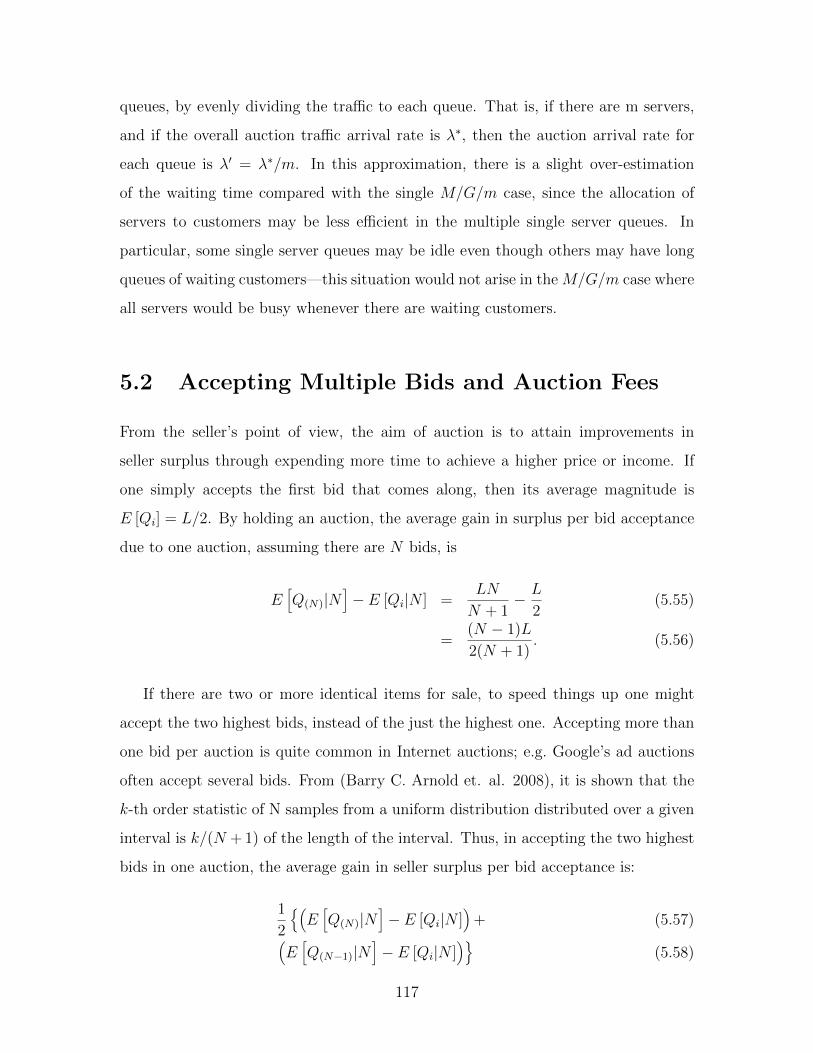
queues, by evenly dividing the traffic to each queue. That is, if there are m servers,

and if the overall auction traffic arrival rate is λ∗, then the auction arrival rate for

each queue is λ′ = λ∗/m. In this approximation, there is a slight over-estimation

of the waiting time compared with the single M/G/m case, since the allocation of

servers to customers may be less efficient in the multiple single server queues. In

particular, some single server queues may be idle even though others may have long

queues of waiting customers—this situation would not arise in the M/G/m case where

all servers would be busy whenever there are waiting customers.

5.2 Accepting Multiple Bids and Auction Fees

From the seller’s point of view, the aim of auction is to attain improvements in

seller surplus through expending more time to achieve a higher price or income. If

one simply accepts the first bid that comes along, then its average magnitude is

E [Qi] = L/2. By holding an auction, the average gain in surplus per bid acceptance

due to one auction, assuming there are N bids, is

E[Q(N)|N

]− E [Qi|N ] =

LN

N + 1− L

2(5.55)

=(N − 1)L

2(N + 1). (5.56)

If there are two or more identical items for sale, to speed things up one might

accept the two highest bids, instead of the just the highest one. Accepting more than

one bid per auction is quite common in Internet auctions; e.g. Google’s ad auctions

often accept several bids. From (Barry C. Arnold et. al. 2008), it is shown that the

k-th order statistic of N samples from a uniform distribution distributed over a given

interval is k/(N + 1) of the length of the interval. Thus, in accepting the two highest

bids in one auction, the average gain in seller surplus per bid acceptance is:

1

2

(E[Q(N)|N

]− E [Qi|N ]

)+ (5.57)(

E[Q(N−1)|N

]− E [Qi|N ]

)(5.58)

117

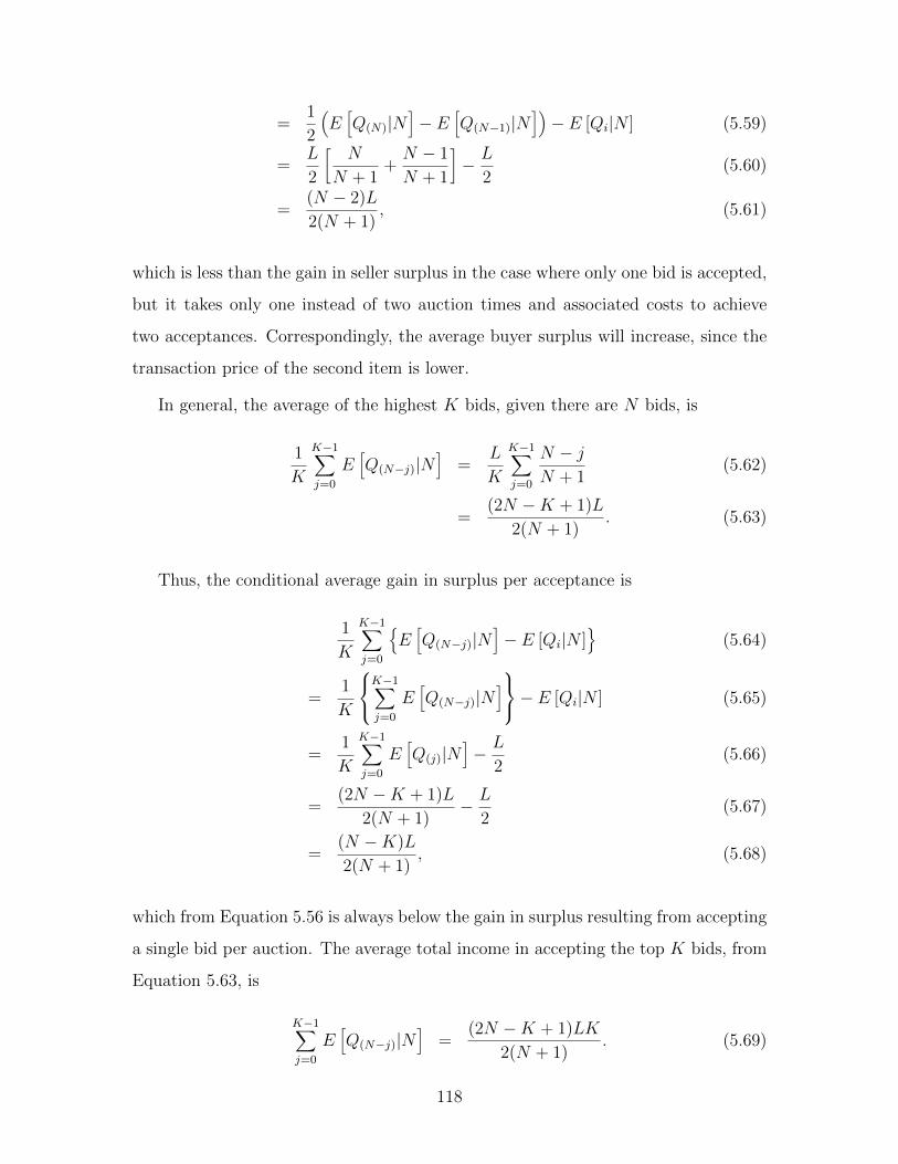
=1

2

(E[Q(N)|N

]− E

[Q(N−1)|N

])− E [Qi|N ] (5.59)

=L

2

[N

N + 1+N − 1

N + 1

]− L

2(5.60)

=(N − 2)L

2(N + 1), (5.61)

which is less than the gain in seller surplus in the case where only one bid is accepted,

but it takes only one instead of two auction times and associated costs to achieve

two acceptances. Correspondingly, the average buyer surplus will increase, since the

transaction price of the second item is lower.

In general, the average of the highest K bids, given there are N bids, is

1

K

K−1∑j=0

E[Q(N−j)|N

]=

L

K

K−1∑j=0

N − jN + 1

(5.62)

=(2N −K + 1)L

2(N + 1). (5.63)

Thus, the conditional average gain in surplus per acceptance is

1

K

K−1∑j=0

E[Q(N−j)|N

]− E [Qi|N ]

(5.64)

=1

K

K−1∑j=0

E[Q(N−j)|N

]− E [Qi|N ] (5.65)

=1

K

K−1∑j=0

E[Q(j)|N

]− L

2(5.66)

=(2N −K + 1)L

2(N + 1)− L

2(5.67)

=(N −K)L

2(N + 1), (5.68)

which from Equation 5.56 is always below the gain in surplus resulting from accepting

a single bid per auction. The average total income in accepting the top K bids, from

Equation 5.63, is

K−1∑j=0

E[Q(N−j)|N

]=

(2N −K + 1)LK

2(N + 1). (5.69)

118

Consider a variation of the basic model, in which the K highest bids are accepted

in one auction. Note that accepting K highest bids requires that there are at least K

arrivals (and of course at least K items for sale), and for meaningful operation, this

requires that T K×Mean Inter-arrival Time or λT K. Removing the condition

on N , and noting that N ≥ K, we have, for the average total income in accepting

the top K bids,

K−1∑j=0

E[Q(N−j)

](5.70)

=∞∑

N=K

LK(2N −K + 1)

2(N + 1)× e−λT (λT )N

N !(5.71)

=LK

2

∞∑N=K

[2− K + 1

N + 1

]× e−λT (λT )N

N !(5.72)

= LK∞∑

N=K

e−λT (λT )N

N !− LK

2λT

∞∑N=K

[K + 1

N + 1

]

×e−λT (λT )N+1

N !(5.73)

= LK∞∑

N=K

e−λT (λT )N

N !−

LK(K + 1)

2λT

∞∑N=K

e−λT (λT )N+1

(N + 1)!(5.74)

= LK

1−K−1∑j=0

e−λT (λT )j

j!

−LK(K + 1)

2λT

1−K∑j=0

e−λT (λT )j

j!

. (5.75)

That is, we have for the expected income IK when we choose to accept K top bids

in a single auction

IK = LK

1−K−1∑j=0

e−λT (λT )j

j!

−LK(K + 1)

2λT

1−K∑j=0

e−λT (λT )j

j!

. (5.76)

We see that for K = 1, the above reduces to Equation 3.4, and for the important

119

special case K = 2, we have

I2 =L

λT

(2λT + λTe−λT − (λT )2e−λT

2+ 3e−λT − 3

). (5.77)

Consider the cost Ω of holding an auction, which may be related to the auction

time and associated costs such as fees paid to the auction site, and payments to

financial intermediaries. We assume that these costs are otherwise not incurred if

the item is sold through other channels. Let the price of a unit of the good be C.

If no auctions are held, then the expected seller surplus would simply be (L/2− C),

where, as indicated from the arguments above, L/2 represents the average value of

the first offer, and we assume that it will be accepted. By holding an auction, the

seller surplus S becomes:

S =L

λT

(λT + e−λT − 1

)− (C + Ω). (5.78)

Thus, the break-even point of holding an auction is given by the improvement in

surplus offset by the auction cost

L

λT

(λT + e−λT − 1

)− L

2= Ω. (5.79)

As the auction extends in time, the expected income rises. Supposing one wishes

to attain a certain level of seller surplus So, then the minimal auction duration T ∗ is

given by the solution to the following equation

S0 =L

λT ∗

(λT ∗ + e−λT

∗ − 1)− (C + Ω). (5.80)

While we may solve for the above using numerical methods, we may obtain closed-

form solutions by using an approximation. An approximation will enable the quick

estimation of auction parameters and economic benefits without going through the

laborious process of numerical solution. We shall use an approximation based on

Equation 3.1. If we remove the condition on N there by replacing N by its average

120

(from the Poisson distribution) of z = λT , we have approximately

E[Q(N)

]∼=

Lz

z + 1. (5.81)

Figure 5-4 compares the average auction income from Equations 3.1 and the above

for L = 100 for different values of z = λT . We see that the approximation is quite

good for moderate to large values of z. For very large values of z, the exact formula

and the approximation are virtually indistinguishable. Using this approximation, the

above becomes

S0 =Lz′

z′ + 1− (C + Ω), (5.82)

giving

z′ =S0 + C + Ω

L− (S0 + C + Ω), (5.83)

and this will provide a reasonable approximation for z′ 1. Thus, the approximate

optimal auction duration T ′ is

T ′ =S0 + C + Ω

λ [L− (S0 + C + Ω)], (5.84)

Letting S0 + C + Ω = 90, L = 100, and λ = 1, and numerically solving Equa-

tion 5.80 provides the exact minimum T ∗ in order to achieve a minimum surplus of

S0 which in this case is found to be T ∗ = 10 (see Figure 5-5). As can be seen from

Figure 5-5, any value of T > 10 will yield at least a surplus of S0. The corresponding

approximate solution gives T ′ = 90/(100 − 90) = 9, which yields an error of just

under 10%. From the seller’s point of view, in order to quickly determine the optimal

T ∗, while avoiding the elaborate procedure of finding a numerical solution to Equa-

tion 5.80, one can simply first solve for T ′, and then add a safety factor to ensure

that the resultant surplus ≥ S0 , which in the present case may be 10%. A higher

safety factor may be used to ensure greater certainty of achieving the required level

121

of minimum surplus.

Next, the overall surplus in accepting K bids per auction is

IK −KC − Ω (5.85)

While the overall surplus in selling K items through K separate auctions would

be

LK

λT

(λT + e−λT − 1

)−K(C + Ω). (5.86)

Thus, it would be more profitable to sell K items in K separate auctions instead

of selling them in a single auction if the expected surplus of the latter is higher, i.e.

LK

λT

(λT + e−λT − 1

)−K(C + Ω) > IK −KC − Ω (5.87)

or

LK

λT

(λT + e−λT − 1

)− (K − 1)Ω > IK (5.88)

0 3 6 9 12 15Average Bids

20

40

60

80

100

120

140Income

ApproximationExact Analysis

Figure 5-4: Comparison of exact analysis and approximation.

122

For the important special case K = 2, the above becomes

2L

λT

(λT + e−λT − 1

)− Ω > I2 (5.89)

and making use of Equation 5.77, this condition simplifies to

ez(

1− zΩ

L

)> 1 + z − z2

2. (5.90)

We see that in terms of magnitude, the left hand side increases exponentially in

z, while the right hand side increases quadratically. Thus, for sufficiently large z, the

left hand side will go negative with a large magnitude, while the right hand side will

also go negative with a comparatively smaller magnitude; consequently the above

inequality will not hold for large z. Thus, when the number of bids is large, it is

always preferable to sell the items in single auctions.

Sometimes, the auction fee structure is such that the auction website would charge

for a certain percentage of the income payment, which for instance is the common

practice of eBay. Denoting by ξ such a percentage, then the overall surplus in accept-

ing K bids per auction is

(1− ξ)IK −KC. (5.91)

In adopting the same approximation as before by suitably replacing N by λT ,

then from Equation 5.69, we have

IK '(2λT −K + 1)LK

2(λT + 1). (5.92)

Using this approximation for the special case K = 2, we have

I2 '(2λT − 1)L

λT + 1, (5.93)

123

so that the overall surplus is approximately

L(1− ξ)(2λT − 1)

λT + 1− 2C. (5.94)

Thus it would be preferable to accept two bids per auction rather than to accept

a single bid in two separate auctions if

2(1− ξ)I1 − 2C < (1− ξ)I2 − 2C, (5.95)

or

2λTL

λT + 1<

2λTL− LλT + 1

, (5.96)

which is never the case for L > 0. Thus, for this particular auction fee structure,

unlike the previous case, it would always be preferable to run two separate auctions

rather than a single auction given that the number of bids is large. In fact, even when

the number of bids is not large, the general validity of this choice can be seen from

Equation 5.69, where the total income from running a single auction is

(1− ξ)IK|N =LK(1− ξ)(2N −K + 1)

2(N + 1), (5.97)

where IK|N signifies the total income conditioning on N . The corresponding quantity

in running K separate auctions is

KI1|N =(1− ξ)NLK

N + 1(5.98)

Thus, it is preferable to run separate auctions if

N

N + 1>

2N −K + 1

2(N + 1)(5.99)

which will be valid whenever K > 1. Thus, for this particular auction fee structure,

unlike the previous one, it is always more advantageous for the seller to sell the items

124

in separate auctions.


20

40

60

80

100

120

140Income

Surplus TargetSeller Surplus

Figure 5-5: Numerical determination of optimal auction duration.

5.3 Surplus Analysis of Soft Close Auctions

For these auctions, a key parameter is s = λα, which is the expected number of bid

arrivals in a window of length α. For the soft close auctions of Algorithm II, the

buyer surplus, from equation (3.16), would be

β(s) = L− L

eλα − 1[eλα − λα− 1] =

sL

es − 1(5.100)

Since

dβ(s)

ds= −L[es(s− 1) + 1]

(es − 1)2< 0 (5.101)

for s ≥ 1, which signifies that there is an average of at least one arrival in the

window of length α, we see that as s increases, the buyer surplus tends to diminish.

Similarly, for the soft close auctions of Algorithm VII, the buyer surplus, from

125

Chapter 4, is

βv(s) = L− 2L

es − 1[sinh(s)− s] =

L(e−s + 2s− 1)

es − 1(5.102)

Now

dβv(s)

ds=L[e−s − 4− es(2s− 3)]

(es − 1)2(5.103)

Since exp(−s) < 1, for s > 0, and the last term is negative if s ≥ 2, combining

these, we conclude that

dβv(s)

ds< 0 for s ≥ 2 (5.104)

The condition s ≥ 2 is a reasonable one, since s represents the average number

of bid arrivals in a window of length α, and for a Vickrey auction, it takes at least

two bids to make it meaningful. This condition implies that as s increases, the buyer

surplus tends to decline.

Since the buyer pays a lower price in Vickrey auctions, it is useful to compare

the buyer surplus of a first-price auction with that of a Vickrey auction. From equa-

tions 5.100 and 5.102 and simplifying, we have for the Vickrey surplus ratio for this

case

βv(s)

β(s)=e−s + 2s− 1

s(5.105)

We see that, by application of L’Hopital’s rule,

βv(s)

β(s)→ 1 as s→ 0 (5.106)

Also, since the Vickrey surplus ratio can be written as

1

ses+ 2− 1

s(5.107)

126

Thus, we see that

βv(s)

β(s)→ 2 as s→∞ (5.108)

The case s→∞ corresponds to a situation where there are a very large number of

bid arrivals in the window of length α, which suggests that the probability of having

no arrivals in that window is very small. Consequently, this means that the auction

will be kept going indefinitely, and thus will last for an effectively infinite amount of

time. This is unlike the fixed auction time situations, where the auction will definitely

finish in a pre-determined amount of finite time.

On the other hand, the seller surplus for the first-price auction is

ξ(s) =L[es − s− 1]

es − 1− C (5.109)

and the seller surplus for the Vickrey auction is

ξv(s) =2L

(es − 1)[sinh(s)− s]− C (5.110)

Thus, the seller surplus reduction by holding a Vickrey auction instead of first-

price auction is

ξ(s)− ξv(s) =L

(es − 1)[e−s + s− 1] (5.111)

For s → 0, we see that, by application of L’Hopital’s rule, that the reduction in

seller surplus → 0. Also, for as s → ∞, we see that each term of Equation 5.111 on

dividing by (es − 1) tends to 0, and so the reduction in seller surplus also → 0.

In Equation 5.108, we see the buyer surplus ratio between the Vickrey and the

first-price auctions is maintained at around two when the number of bids is large, when

there is the same average number of bids s in both cases. However, since Vickrey

auctions tend to encourage greater bidder participation, so that it is useful to compare

the buyer surplus ratio when the average number of bids in the Vickrey auctions is

127

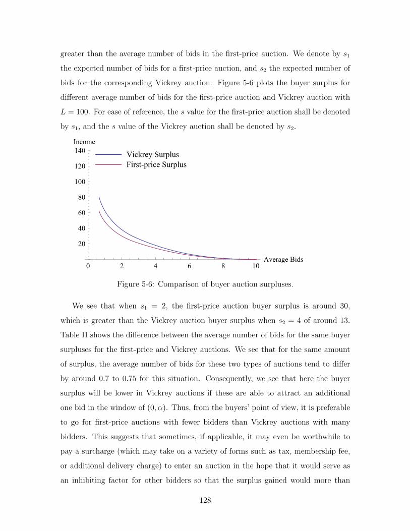
greater than the average number of bids in the first-price auction. We denote by s1

the expected number of bids for a first-price auction, and s2 the expected number of

bids for the corresponding Vickrey auction. Figure 5-6 plots the buyer surplus for

different average number of bids for the first-price auction and Vickrey auction with

L = 100. For ease of reference, the s value for the first-price auction shall be denoted

by s1, and the s value of the Vickrey auction shall be denoted by s2.


20

40

60

80

100

120

140Income

First-price SurplusVickrey Surplus

Figure 5-6: Comparison of buyer auction surpluses.

We see that when s1 = 2, the first-price auction buyer surplus is around 30,

which is greater than the Vickrey auction buyer surplus when s2 = 4 of around 13.

Table II shows the difference between the average number of bids for the same buyer

surpluses for the first-price and Vickrey auctions. We see that for the same amount

of surplus, the average number of bids for these two types of auctions tend to differ

by around 0.7 to 0.75 for this situation. Consequently, we see that here the buyer

surplus will be lower in Vickrey auctions if these are able to attract an additional

one bid in the window of (0, α). Thus, from the buyers’ point of view, it is preferable

to go for first-price auctions with fewer bidders than Vickrey auctions with many

bidders. This suggests that sometimes, if applicable, it may even be worthwhile to

pay a surcharge (which may take on a variety of forms such as tax, membership fee,

or additional delivery charge) to enter an auction in the hope that it would serve as

an inhibiting factor for other bidders so that the surplus gained would more than

128

cover the surcharge. In addition, individually, it is worth noting that with either of

these two auction types, the buyer surplus drops steeply at first, and the drop slows

down when the average number of bids becomes large.

Buyer Surplus Average Numberof bids (Vickrey)

Average Numberof bids (First-Price)

Difference in theAverage Numberof Bids

50 1.97 1.26 0.7145 2.15 1.43 0.7240 2.35 1.62 0.7335 2.57 1.83 0.7430 2.81 2.06 0.7525 3.09 2.34 0.7520 3.41 2.66 0.7515 3.81 3.06 0.7510 4.36 3.61 0.755 5.25 4.51 0.74

Table 5.2: Comparison of the average number of bids for equal surplus.

From the seller’s point of view, the seller surplus between the first-price auction

and the corresponding Vickrey auction would be

ξ(s1)− ξv(s2) < 0 (5.112)

if

es1 − s1 − 1

es1 − 1<

2[sinh(s2)− s2]

(es2 − 1)(5.113)

Figure 5-7 plots the seller surplus for both types of auctions for C = 20. We see

that the two surplus curves tend to be parallel, separating by below one bid, initially.

For example, to attain a surplus of 50, we see that s1 = 2.06 and s2 = 2.81 with

s2− s1 = 0.75. Hence, if the seller is confident that by running a Vickrey auction, an

average of one additional bid is attracted to the auction, then the expected surplus of

the a Vickrey auction would be higher, and thus it would be better to run a Vickrey

auction instead of a first-price auction.

As for Algorithm V, if the buyer is aiming for a surplus of ξ, then B should be

129


20

40

60

80

100

120

140Income

First-price SurplusVickrey Surplus

Figure 5-7: Comparison of seller auction surpluses.

chosen such that

C + ξ =BL

B + 1(5.114)

Solving for B gives

B = [C + ξ

L− (c+ ξ)] (5.115)

Since the above is generally not an integer, the ceiling function

[C + ξ

L− (c+ ξ)] (5.116)

should yield a surplus not less than ξ, since we have shown earlier that the auction

income is an increasing function of B.

Similarly, for Algorithm X, the parameter B should satisfy

C + ξ =(B − 1)L

B + 1(5.117)

130

giving

B = [L+ C + ξ

L− (C + ξ)] (5.118)

which would yield a surplus not less than ξ. For example, if C + ξ = 80, L = 100,

then B in Algorithm V should be set to 4, while it should be set to 9 in Algorithm X.

From the buyers’ perspective, the buyer surplus for the first-price auction is

β = L− BL

B + 1=

L

B + 1(5.119)

while that for the Vickrey auction is

βv = L− (B − 1)L

B + 1=

2L

B + 1(5.120)

showing again that the buyer surplus for the Vickrey auction is twice that for the

first-price auction.

5.4 Surplus Analysis of Auctions with Threshold

Termination

For auctions with threshold termination, we have shown earlier that their average

duration is generally shorter than the corresponding auctions without the threshold

termination. For these auction algorithms, the arriving bids are probabilistically the

same as for the corresponding auctions without threshold termination. The only

difference between the two is that it would terminate prematurely upon receiving a

certain bid, otherwise the auction would continue through to usual completion. As we

have shown earlier, longer auctions tend to yield higher incomes, and since auctions

without threshold termination tend to run longer, their auction income is also higher

(of course, in the event that there is no arrival from the Λ-stream, the two auctions

would be identical in both duration and income), a property also evident from the

income graphs of earlier chapters.

131

The setting of the threshold M by the sellers is related to the sellers’ view on

the magnitude of an acceptable surplus. If a seller regards ξ is an acceptable level

of minimum surplus, then the seller may set M = C + ξ. If the auction is finished

through threshold termination, then since the conditional income for this situation is

(M + L)/2, which is higher than M , then the seller would expect to fetch a surplus

exceeding ξ. However, as we have just indicated, such a surplus will still on average

be lower than the expected surplus were the auction be allowed to run its full course,

since the latter possibility will result in a longer auction and hence attaining higher

average income. For example, if the acceptable level of minimum surplus ξ is 30, then

for C = 20, we have M = 50 , and the expected auction income for L = 100, α = 3, is

plotted in Figure 5-9. We see that the minimum acceptable surplus is attained when

the arrival rate is 0.5, and when the arrival rate is 1, the surplus reaches 50. From

Chapter 3, the average auction income of Algorithm IV,

E[Q′M ] =p1M [1− Λ′α

(eΛ′α−1)] + p2[M+L

2]

P1 + P2

(5.121)

is a convex combination of two component incomes. The first one

M [1− Λ′α

(eΛ′α − 1)] (5.122)

is bounded above by M , since

Λ′α

(eΛ′α − 1)< 1 (5.123)

which can be seen on expanding exp(Λ′α). On the other hand, the second one

[M + L

2] (5.124)

is bounded below by M , so that the second income is always greater than the first

132

income. Therefore the average auction income is

E[Q′M ] ≤p1[M+L

2] + p2[M+L

2]

p1 + p2

= [M + L

2] (5.125)

which in this case is (50+100)/2=75. We see from Figure 5-9 that the auction

income is always below 75. Indeed, as the bid rate increases, s→∞ and so p1 = es →

0, the average auction income gradually approaches this bound. This is intuitively

reasonable and is to be expected since when there is a large number of bids arriving,

the chance of one of them meeting the threshold requirement would accordingly be

high, and so the auction terminates at (M + L)/2.

As for Algorithm III, the average auction income, from Chapter 3, may be written

as

E[QM ] = e−ΛTM [1− 1− e−Λ′T

Λ′T] + (1− e−ΛT )[

M + L

2] (5.126)

In order for the first component income to be less than M , the condition

(1− e−Λ′T )

Λ′T< 1 (5.127)

has to be satisfied, which is equivalent to

(eΛ′T − 1) < Λ′TeΛ′T (5.128)

Expanding both sides, we have

Λ′T +(Λ′T )2

2!+

(Λ′T )3

3!+ ... < Λ′T + (Λ′T )2 +

Λ′T 3

2!+

Λ′T 4

3!+ . . . (5.129)

which is seen to be true on term by term comparison and noting that Λ′T > 0.

Thus the first component income in E[Q(M)

]is less than M ; obviously, the second

income component is greater than M , and so

E[QM ] ≤ e−ΛT [M + L

2] + (1− e−ΛT )[

M + L

2] = [

M + L

2] (5.130)

133

A plot of the average auction income for C = 30, ξ = 40, L = 100, T = 10, is shown

in Figure 5-8. We see that the acceptable surplus is reached when the bid rate is

around 0.34, and it converges to, but bounded by, 85 as the bid rate increases.

0 0.5 1.0 1.5 2.0 2.5Bid Rate

20

40

60

80

100

120

140Income

Asymptotic Bound

Cost

Acceptable Surplus and Cost

Figure 5-8: Seller Surplus for Algorithm III.

0 0.5 1.0 1.5 2.0 2.5Bid Rate

20

40

60

80

100

120

140Income

Asymptotic Bound

Cost

Acceptable Surplus and Cost

Figure 5-9: Seller Surplus for Algorithm IV.

As for Vickrey auctions with threshold termination, the same auction income

bound of (M + L)/2 also applies since the income component from non-threshold

termination here is even lower than that of the first-price auction. By the same

argument, when the bid rate is large, the chance of termination by reaching M would

134

be high, and so the income upper bound of (M +L)/2 is likely to be attained. Thus,

for auctions with reasonably strong participation, there is little difference between

the first-price auctions and Vickrey auctions in terms of surplus.

5.5 Summary

From both the buyers and sellers points of view, apart from successfully buying

or selling the goods or services, a key objective is to reap maximum benefits from

auctions in the form of economic surpluses. Compared with buyers, sellers tend to

have greater flexibility and control over how an auction is being conducted. They

can choose the duration parameters of the auctions, as well as whether to run them

as first-price or Vickrey auctions. In addition, they can choose to incorporate the

buy-it-now option to possibly shorten the auction duration once a required level

of surplus is reached. We have analysed and compared the surpluses from both the

buyers and sellers perspectives for the different auction algorithms. From the analysis

performed, it is found that it would often be advantageous for sellers to run Vickrey

auctions rather than first-price auctions. Another auction design option available to

sellers when multiple items are for sale is whether or not to accept more than one

bid per auction. Doing so will obviously save time and effort, but will also lower the

average seller surplus. However, depending on the auction fee structure, accepting

more than one bid in an auction can sometimes yield greater economic benefits than

holding separate auctions. A factor which neither the sellers nor buyers have any

real control is the bid rate. From the buyers’ point of view, having a high bidder

participation rate is always disadvantageous for buyer surplus. Thus, it is sometimes

preferable for buyers to participate in less crowded first-price auctions than crowded

Vickrey auctions. Indeed, inhibiting participation from other bidders is so important

that it may sometimes pay to opt for those auctions with surcharge (if such choice

is applicable), in the expectation that the gain in surplus will more than cover the

surcharge. Of course, if such information is unavailable, then the buyers should always

opt for the Vickrey auction which generally yields twice the surplus compared with

135

first-price auctions.

136

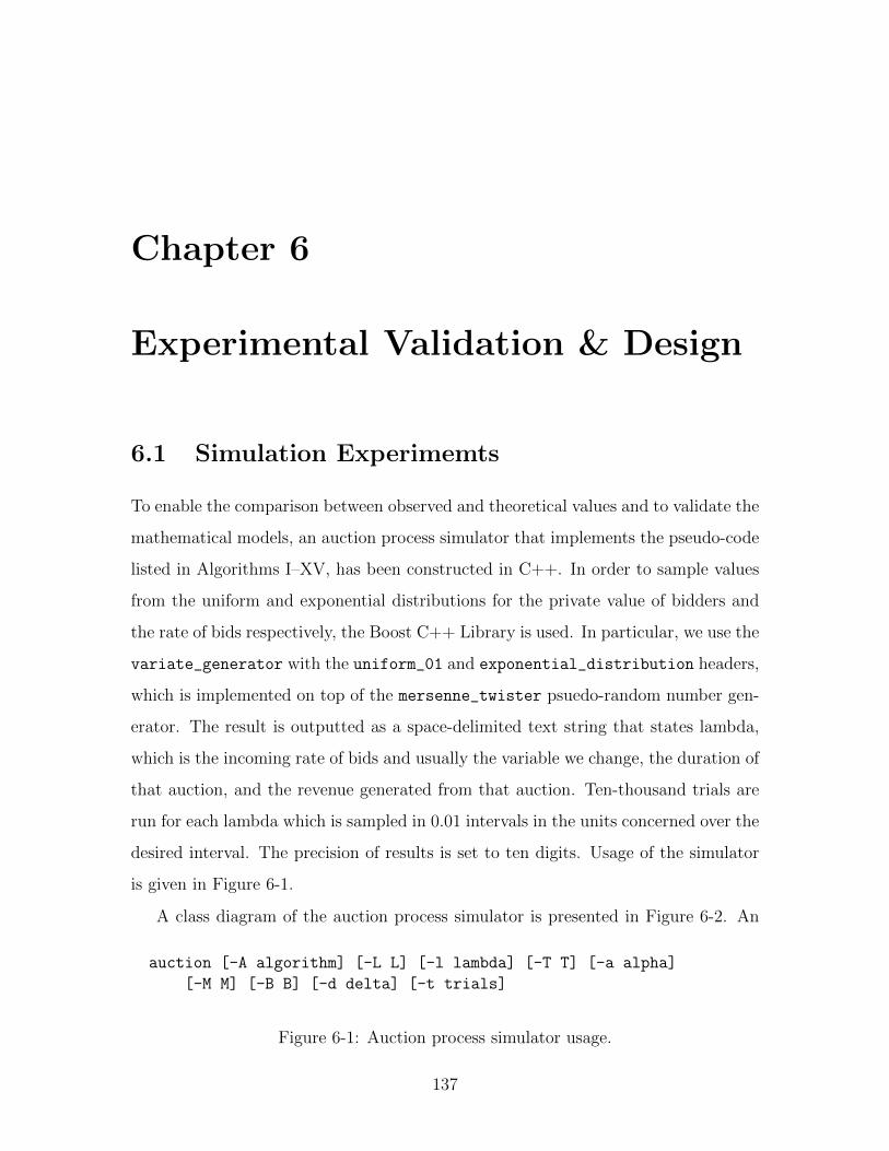
Chapter 6

Experimental Validation & Design

6.1 Simulation Experimemts

To enable the comparison between observed and theoretical values and to validate the

mathematical models, an auction process simulator that implements the pseudo-code

listed in Algorithms I–XV, has been constructed in C++. In order to sample values

from the uniform and exponential distributions for the private value of bidders and

the rate of bids respectively, the Boost C++ Library is used. In particular, we use the

variate_generator with the uniform_01 and exponential_distribution headers,

which is implemented on top of the mersenne_twister psuedo-random number gen-

erator. The result is outputted as a space-delimited text string that states lambda,

which is the incoming rate of bids and usually the variable we change, the duration of

that auction, and the revenue generated from that auction. Ten-thousand trials are

run for each lambda which is sampled in 0.01 intervals in the units concerned over the

desired interval. The precision of results is set to ten digits. Usage of the simulator

is given in Figure 6-1.

A class diagram of the auction process simulator is presented in Figure 6-2. An

auction [-A algorithm] [-L L] [-l lambda] [-T T] [-a alpha]

[-M M] [-B B] [-d delta] [-t trials]

Figure 6-1: Auction process simulator usage.

137

Internet auction website contains a number of buyers and sellers and runs multiple

auctions, each of which contains a subset of the auction website’s buyers and sellers

exchanging money for lots of goods and services. Each auction has a set of parameters

which equate to the parameters of the various algorithms.

Buyers have a utility function for each lot that is present at the auction website,

and if the utility gained from buying a lot at a specific price is greater than that

derived from holding the money, or using that lot to buy another lot, then the buyer

will offer to bid for that lot in an auction. Both the utility of a win and a loss is

required in determining how close a buyer should bid to his true valuation. If the loss

of an auction is very costly, the buyer should bid the true valuation of the lot straight

away, instead of trying to augment his utility by obtaining the lot at a lower price

that he was willing to pay for it. The confidence that a buyer has in his valuation

determines whether the valuation will be adjusted in the face of significantly higher or

lower bids from other bidders present in the auction. A high confidence in the values

means that the list of utility for each lot remains the same throughout an auction,

while a lower confidence may mean that the auction itself is, to a certain extent, a

price discovery mechanism for the bidder and his utility of obtaining the lot may vary

in accordance with the current bid levels. In the same way, the seller also has lists of

utilities and confidences, as well as a value for reputation which may result in a price

discount or premium in an auction depending on factors that may be external to the

lot, e.g. timeliness of delivery. Currently there are a few features listed in the class

diagram that have not been fully implemented such as the buyer and seller utilities,

confidence in their utility and their ratings at the auction website.

The class diagram uses standard Unified Modelling Language (UML) notation

and shows different classes, their attributes and methods, and how they inter-relate.

Private attributes and methods, which are known only to the class itself and to

no other classes, are preceded with a (-) symbol, while, if public, preceded by a

(+) symbol. There exists four main classes: the Auction Website, the Auction, the

Buyer and the Seller. Classes connected by just a line indicate association, while a

hollow diamond, aggregation, i.e. “Class A has Class B”, with the hollow diamond-

138

end connecting to the container class (A). A solid diamond, on the other hand, means

composition, which is a stronger version of association, with the associated class often

unable to exist if the class to which it is associated is destroyed. Numbers at two ends

of the lines, indicate multiplicity, or the number of classes that participate in that

association, e.g. “1..*” indicates an association that relates to “1 or more” classes.

Thus, in Figure 6-2, an auction house/website runs one or more auctions which have

parameters determining whether it is first-price or k-price, whether it has a minimum

or maximum limit on the number of bids, and can either be a fixed time or variable

time auction. Furthermore, each auction takes place by auctioning off a lot which is

transferred from one owner (the seller) to another owner (the buyer), each of which

has an associated reputation and wealth. Sellers can also set a reserve price on a lot,

while each buyer has a valuation of each lot (consisting of an associated utility and

confidence in that utility), which determines the amounts that the buyer should bid

for those lots.

AuctionHouse / Website

admit (entity) depart (entity)

Entity entity_id: int name: string money: int rating: int

Seller offer (lot)

Auction auction_id: int first_price: bool min_bids: int max_bids: int start ()

Buyer bid (lot, price)

Lot lot_id: int name: string reserve_price: int sold_price: int sold_date: date

1..*runs1

auctions1 1..*

facilitates1 1..*

owned1..*

1

0..*1owns

Valuation utility: int confidence: float

*

*

Fixed Time duration: time

Variable Time inactivity: time

Figure 6-2: UML class diagram for the auction process simulator.

From the simulation experiments, the theoretical and simulation results are com-

139

0 1 2

40

80

120

160

Bid Rate

Duration

Theoretical

α = 1.0α = 2.0

α = 3.0


pared, and the agreements are all extremely good. A sample of the graphs comparing

the theoretical and simulation results is given below, where the thick curves are those

obtained from theory and the thin curves are those obtained by simulation.

140

0 1 2

40

80

120

160

Bid Rate

Duration

Theoretical

α = 1.0α = 2.0

α = 3.0


0 1 2

2

4

6

8

Bid Rate

Duration

Theoretical

M = 20.0M = 40.0M = 60.0M = 80.0

Figure 6-5: Average auction duration of fixed-time first-price forward auction withmaximum threshold termination.

141

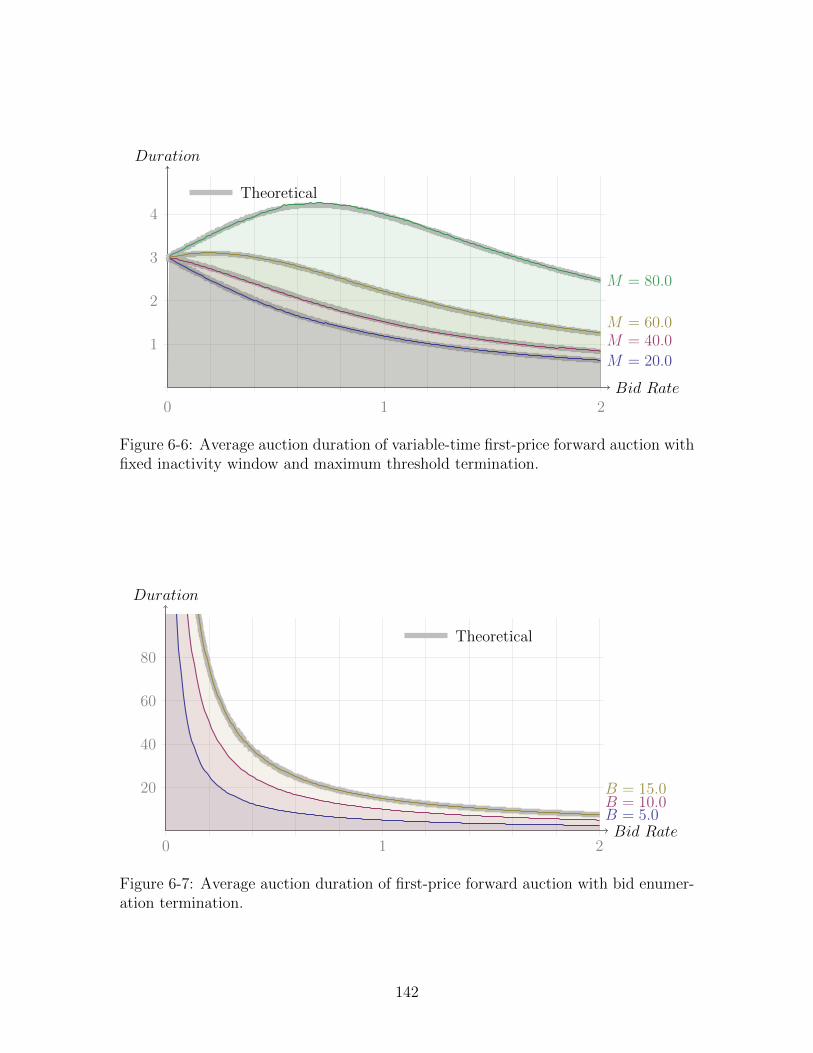
0 1 2

1

2

3

4

Bid Rate

Duration

Theoretical

M = 20.0

M = 40.0M = 60.0

M = 80.0

Figure 6-6: Average auction duration of variable-time first-price forward auction withfixed inactivity window and maximum threshold termination.

0 1 2

20

40

60

80

Bid Rate

Duration

Theoretical

B = 5.0B = 10.0B = 15.0

Figure 6-7: Average auction duration of first-price forward auction with bid enumer-ation termination.

142

0 2 4 6 8 10

92

94

96

98

Bid Rate

Income

Theoretical

T = 5.0

T = 10.0T = 15.0

Figure 6-8: Average auction income of fixed-time first-price forward auction.

0 1 2

20

40

60

80

Bid Rate

Income

Theoretical

α = 1.0

α = 2.0α = 3.0

Figure 6-9: Average auction income of variable-time first-price forward auction withfixed inactivity window.

143

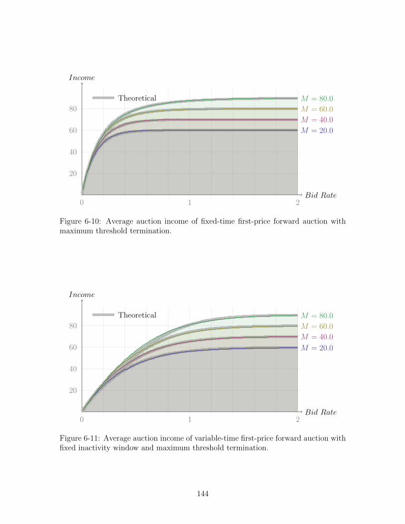
0 1 2

20

40

60

80

Bid Rate

Income

Theoretical

M = 20.0

M = 40.0

M = 60.0

M = 80.0

Figure 6-10: Average auction income of fixed-time first-price forward auction withmaximum threshold termination.

0 1 2

20

40

60

80

Bid Rate

Income

Theoretical

M = 20.0

M = 40.0

M = 60.0

M = 80.0

Figure 6-11: Average auction income of variable-time first-price forward auction withfixed inactivity window and maximum threshold termination.

144

0 2 4 6 8 10

92

94

96

98

Bid Rate

Income

Theoretical

T = 5.0

T = 10.0

T = 15.0

Figure 6-12: Average auction income of fixed-time Vickrey forward auction.

0 1 2

20.0

40.0

60.0

80.0

Bid Rate

Income

Theoretical

α = 1.0

α = 2.0

α = 3.0

Figure 6-13: Average auction income of variable-time Vickrey forward auction withfixed inactivity window.

145

0 1 2

20.0

40.0

60.0

80.0

Bid Rate

Income

Theoretical

M = 20.0

M = 40.0

M = 60.0

M = 80.0

Figure 6-14: Average auction income of fixed-time Vickrey forward auction withmaximum threshold termination.

0 1 2

20.0

40.0

60.0

80.0

Bid Rate

Income

Theoretical

M = 20.0

M = 40.0

M = 60.0

M = 80.0

Figure 6-15: Average auction income of variable-time Vickrey forward auction withfixed inactivity window and maximum threshold termination.

146

0 1 2

60

70

80

90

Bid Rate

Income

Theoretical

B = 5.0

B = 10.0

B = 15.0

Figure 6-16: Average auction income of Vickrey forward auction with bid enumerationtermination.

147

0 2 4 6 8 10

2

4

6

8

Bid Rate

Income

Theoretical

T = 5.0

T = 10.0T = 15.0

Figure 6-17: Average auction income of fixed-time last-price reverse auction.

6.2 Comparison with eBay Auction Data

Actual Internet auction data are obtained from eBay for comparison purposes. It is

found that with many of the auctions, the number of bids is not high, often falling

below ten. Among the most popular items are iPhone 4 with different colours, spec-

ifications and varying conditions. eBay auctions tend to be fixed time auctions, and

we extracted the data from five eBay iPhone4 auctions that have at least 15 bids.

These detailed auction data are given in Appendix A.

It must be emphasised that actual live data has a number of drawbacks. Firstly,

unlike simulation experiments, these experimental observations are not reproducible—

they can be somewhat haphazard due to the fact that the prevailing conditions gov-

erning the underlying processes are not experimentally repeatable. In fact, even

in well-studied models such as those in queueing theory, it is generally unlikely to

have the measurements taken from an actual queueing situation exactly matching

the established theoretical results. Secondly, unlike simulation experiments, the ex-

perimental conditions are not under the control of the experimenter.

From these eBay data, we wish to examine the bid arrival pattern, the distribution

of bid values, and the auction income.

We first examine the bid arrival pattern, and the relevant data are given in Ta-

148

0 1 2

20.0

40.0

60.0

80.0

Bid Rate

Income

Theoretical

α = 1.0

α = 2.0α = 3.0

Figure 6-18: Average auction income of variable-time last-price reverse auction withfixed inactivity window.

0 1 2

20.0

40.0

60.0

80.0

Bid Rate

Income

Theoretical

M = 20.0

M = 40.0

M = 60.0

M = 80.0

Figure 6-19: Average auction income of fixed-time last-price reverse auction withminimum threshold termination.

149

0 1 2

20.0

40.0

60.0

80.0

Bid Rate

Income

Theoretical

M = 20.0

M = 40.0

M = 60.0

M = 80.0

Figure 6-20: Average auction income of variable-time last-price reverse auction withfixed inactivity window and minimum threshold termination.

0 1 2

4

8

12

16

Bid Rate

Income

TheoreticalB = 5.0

B = 10.0

B = 15.0

Figure 6-21: Average auction income of last-price reverse auction with bid enumera-tion termination.

150

ble 6.1. We note that for Poisson arrival, the inter-arrival time distribution has a

coefficient of variation of one.

From Table 6.1, we see that for auction A1, the coefficient of variation of the

inter-arrival time of 1.01 is very close to one indeed, with an error percentage of

under 1%. For auction A3, the coefficient of variation of the inter-arrival time of 0.93

is also close to one, with an error percentage of around 7.5%. For auction A5, the

coefficient of variation of the inter-arrival time of 1.2 is higher, but the error percentage

of 16.7% is not excessive. The departure from the exponential inter-arrival time is

more pronounced, however, in the cases of auctions A2 and A4. The average of the

observed coefficients of variation of the inter-arrival time is 1.166, which deviates

from the theoretical value by 16.6%, and the average error is 15.23%. However, it

is interesting to note that, in the case of auction A4, when the arrival of the first

three bids are not included, the inter-arrival time of the remaining 18 bids has a

coefficient of variation of 1.032, which is rather close to the Poisson coefficient of

variation. Moreover, in the case of auction A2, when the arrival of the first three bids

are not included, the inter-arrival time of the remaining 14 bids has a coefficient of

variation of 1.116, and also, in the case of auction A5, when the arrival of the three

bids are not included, the inter-arrival time of the remaining 12 bids has a coefficient

of variation of 1.017. It would appear particularly that, in the cases of auctions A4

and A5, while their overall bid arrival patterns are not strictly Poisson, they seem to

converge to the Poisson pattern when some initial transient effects are disregarded.

Column 6 of Table 6.1 shows the coefficients of variation after the transient effects

of A2, A4, and A5 are adjusted with the inter-arrival times of the first three bids

disregarded. The adjusted coefficients of variation have a mean of 1.022, which shows

little deviation from the theoretical average Poisson coefficient of variation of one,

while the corresponding average error is around 4.8%. Column 7 of Table 6.1 shows

the coefficients of variation after the transient effects of all the five auctions are

adjusted with the inter-arrival times of the first three bids disregarded. The adjusted

coefficients of variation have a mean of 1.004, which is very close to one indeed, while

the corresponding average error is around 6.7%. From these observations, it is possible

151

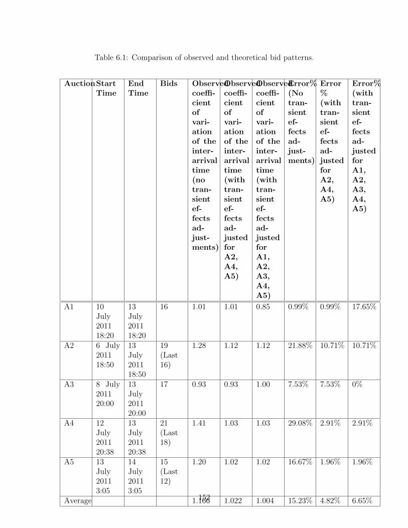
Table 6.1: Comparison of observed and theoretical bid patterns.

AuctionStartTime

EndTime

Bids Observedcoeffi-cientofvari-ationof theinter-arrivaltime(notran-sientef-fectsad-just-ments)

Observedcoeffi-cientofvari-ationof theinter-arrivaltime(withtran-sientef-fectsad-justedforA2,A4,A5)

Observedcoeffi-cientofvari-ationof theinter-arrivaltime(withtran-sientef-fectsad-justedforA1,A2,A3,A4,A5)

Error%(Notran-sientef-fectsad-just-ments)

Error%(withtran-sientef-fectsad-justedforA2,A4,A5)

Error%(withtran-sientef-fectsad-justedforA1,A2,A3,A4,A5)

A1 10July201118:20

13July201118:20

16 1.01 1.01 0.85 0.99% 0.99% 17.65%

A2 6 July201118:50

13July201118:50

19(Last16)

1.28 1.12 1.12 21.88% 10.71% 10.71%

A3 8 July201120:00

13July201120:00

17 0.93 0.93 1.00 7.53% 7.53% 0%

A4 12July201120:38

13July201120:38

21(Last18)

1.41 1.03 1.03 29.08% 2.91% 2.91%

A5 13July20113:05

14July20113:05

15(Last12)

1.20 1.02 1.02 16.67% 1.96% 1.96%

Average 1.166 1.022 1.004 15.23% 4.82% 6.65%152

Table 6.2: Comparison of observed and theoretical bid value patterns.

Auction Start Time End Time Bids Observedcoeffi-cientofvari-ationof bidvalue

Error %

A1 10 July 2011 18:20 13 July 2011 18:20 16 0.68 15.10%A2 6 July 2011 18:50 13 July 2011 18:50 19 0.64 9.79%A3 8 July 2011 20:00 13 July 2011 20:00 17 0.61 5.35%A4 12 July 2011 20:38 13 July 2011 20:38 21 0.55 4.97%A5 13 July 2011 3:05 14 July 2011 3:05 15 0.62 6.88%Average 0.62 8.42%

to conclude that the Poisson arrival assumptions is a valid one for at least some of

the actual auction processes, while it can be employed as a useful approximation for

some others.

We next examine the bid value patterns, and the results are given in Table 6.2.

We note that, for uniformly distributed bid values, the coefficient of variation is 0.58.

We see that, with the exception of auction A1, all the other auctions have for the

coefficient of variation of the bid value reasonably close to the theoretical value of 0.58,

all having below 10% error. For auctions A3 and A4, their coefficients of variation

of the bid value are quite close to the theoretical value of 0.58, having only around

5% error. For auction A1, its coefficient of variation of the bid value has a slightly

higher error percentage of 15.1%, but is not excessive. The average of the observed

coefficient of variation of the bid value is 0.62, which deviates from the theoretical

value of 0.58 by 6.88%, and the average error is 8.42%. From these observations, it

is possible to conclude that using uniformly distributed bid values generally provides

a reasonable working approximation for the study of Internet auction processes.

We also compare the auction income for both the first-price forward auction and

the Vickrey auction. The parameter L is estimated from Equation 3.1 with N taken

153

Table 6.3: First-price forward auction income.

Auction Start Time End Time Bids Observedauc-tionin-come

Theoreticalauc-tionin-come

Error %

A1 10 July 2011 18:20 13 July 2011 18:20 16 575 572.8 0.4%A2 6 July 2011 18:50 13 July 2011 18:50 19 420 418.8 0.3%A3 8 July 2011 20:00 13 July 2011 20:00 17 475 473.4 0.3%A4 12 July 2011 20:38 13 July 2011 20:38 21 540 538.8 0.2%A5 13 July 2011 3:05 14 July 2011 3:05 15 525 522.7 0.4%

Table 6.4: Vickrey auction income.

Auction Start Time End Time Bids Observedauc-tionin-come

Theoreticalauc-tionin-come

Error %

A1 10 July 2011 18:20 13 July 2011 18:20 16 565 534.6 5.4%A2 6 July 2011 18:50 13 July 2011 18:50 19 410 395.6 3.5%A3 8 July 2011 20:00 13 July 2011 20:00 17 470 443.7 5.6%A4 12 July 2011 20:38 13 July 2011 20:38 21 530 511.8 3.4%A5 13 July 2011 3:05 14 July 2011 3:05 15 515 485.3 5.8%

to be the number of bids. Since λT gives the average number of bids, the parameter

λ is estimated by the number of bids divided by the auction duration. The results

are given in Tables 6.3 and 6.4. We see that the agreement is generally good, with

error percentage below 6%.

154

Table 6.5: Simulation using eBay parameters for first-price forward auctions.

Auction L λ T Auctionin-come(sim-ula-tion)

Auctionin-come(eBay)

Error %

A1 610.97 0.222 72 572.75 575 0.39%A2 442.11 0.113 168 418.82 420 0.28%A3 502.94 0.142 120 473.42 475 0.33%A4 565.71 0.875 24 538.77 540 0.23%A5 560.00 0.625 24 522.66 525 0.44%

Table 6.6: Simulation using eBay parameters for Vickrey auctions.

Auction L λ T Auctionin-come(sim-ula-tion)

Auctionin-come(eBay)

Error %

A1 610.97 0.222 72 534.52 565 5.39%A2 442.11 0.113 168 395.53 410 3.53%A3 502.94 0.142 120 443.91 470 5.55%A4 565.71 0.875 24 511.83 530 3.43%A5 560.00 0.625 24 485.33 515 5.76%

6.3 Simulations using eBay-determined Parame-

ters

We also carry out simulations using the parameters as estimated from the eBay data

above and the results are given in Table 6.5 and Table 6.6. We also see that the

agreement is generally good.

155

Chapter 7

Sensitivity Analysis of the Auction

Income With Respect to Different

Independent Values Distributions

As we have seen, the Independent Private Values (IPV) model plays a fundamental

role in the analyses of Internet auction performance. This model assumes privacy and

independence, meaning that the private values of buyers are drawn from a common

distribution, or in probabilistic terms, the series of values are independent and identi-

cally distributed. In this chapter, we shall study the sensitivity of the auction income

with respect to different Independent Values Distributions and their appropriateness

for Internet auctions. We shall also provide analytic approximations to the auction

income for different Independent Values Distributions by introducing the damping

factor which modifies the bid rate.

7.1 Importance of the Uniform Distribution for

Independent Private Values

The uniform distribution for private values is commonly employed in auction studies

(Katok and Kwasnica, 2008). It possesses the following desirable features that are

157

widely used to characterise Internet auction behaviour.

1. It is naturally capped by a finite value: in most auctions, the private values do

not go to infinity but is bounded by a certain upper limit. Since bids can often

start at a very low value, the range of values permitted by uniformly private

values may be presented by (0, L), so that with the probability that a bid falling

into a small value interval is given by Pr[x < Qj < x+ ∆x] = ∆x/L.

2. It represents that no information is available and no bias exists concerning the

inclinations and behaviour of the underlying bidder group, as well as no inter-

action or correlation between bids: any value is possible and they happen with

equal probability. This property is also useful in expressing a wide cross-section

of bidder valuation spreading over different geographical regions, disparate cul-

tures, personal preferences and perceptions—typically found on the Internet—

and with little or no communication or agreements among the bidders.

Key performance metrics are the average income per auction and the average

duration of an auction. Since for hard close auctions, the auction duration is fixed,

this quantity is of interest mainly for the soft close case, where the duration is a

random variable. For each parameter setting, we carry out 100 auction experiments

and the measurements collected are averaged. Figure 7-1 shows the average auction

income for different values of λ for hard close auctions when T = 10, and L = 100.

We see that the increase in bid rate up to about λ = 1 produces rather steep average

auction income improvement. There seems to be a critical bid rate at around λ = 1,

above which the improvement in income becomes less pronounced.

Figure 7-2 shows how auction income varies for soft close auctions with λ for

α = 1, 2, 3 and 4. We see that average auction income increases gradually for small

values of λ, but accelerates for large values. As the bid rate increases, there is reduced

chance of a no bid interval occurring, and the difference between α = 1 and α = 4

tends to widen as λ → 1, but slowly narrows afterwards, especially between α = 2,

α = 3 and α = 4. Depending on the specified length of the no bid interval α, the

auction duration for soft close auctions can show considerable divergence for high bid

158

0 2 4 6 8 10Bid Rate (Bids/s)

20

40

60

80

100

120

140Income

Figure 7-1: Auction income for uniformly distributed private values for hard closeauctions.

rate, which is shown in Figure 7-3. We observe that for larger values of α (e.g. α = 4),

it can shoot up to very large values for high bid rates, which seems to be due the fact

that under such circumstances, having no arriving bid in an interval of α = 4 becomes

increasingly unattainable, leading to almost an indefinite continuation of the auction.

0 0.5 1.0 1.5 2.0 2.5Bid Rate (Bids/s)

20

40

60

80

100

120

140Income

α = 4α = 3α = 2α = 1

Figure 7-2: Auction income for uniformly distributed private values for soft closeauctions.

159

0 0.5 1.0 1.5 2.0 2.5Bid Rate (Bids/s)

200

400

600

800

1000

1200

1400Duration

α = 4α = 3α = 2α = 1

Figure 7-3: Auction duration for uniformly distributed private values for soft closeauctions.

7.2 Exponentially distributed private values

The exponential distribution µe−µv is one of the most widely used distributions in

stochastic modelling. Compared with the uniform distribution, it has an added nat-

ural advantage of representing private values since private values are not allowed to

go negative, and the exponential random variable is always positive. Since for the

exponential distribution, the smaller values has a higher probability of occurring than

higher values, i.e. for u < v and an arbitrary interval of length k,

Pr [u ≤ Qi ≤ u+ k] =∫ u+k

uµe−µtdt

>

Pr [v ≤ Qi ≤ v + k] =∫ v+k

vµe−µtdt,

which is a consequence of the inequality e−µu > e−µv. Thus the exponential private

values distribution represents a situation where people are looking for bargains from

the auction, since the lower values are favoured. Figures 7-4 and 7-5 give the auction

performance of the exponentially distributed private values; for effective comparison

with the uniformly distributed private values, here we set 1/µ = L/2 = 50. The

graph for the auction duration for soft close auctions is omitted as it is the same as

160

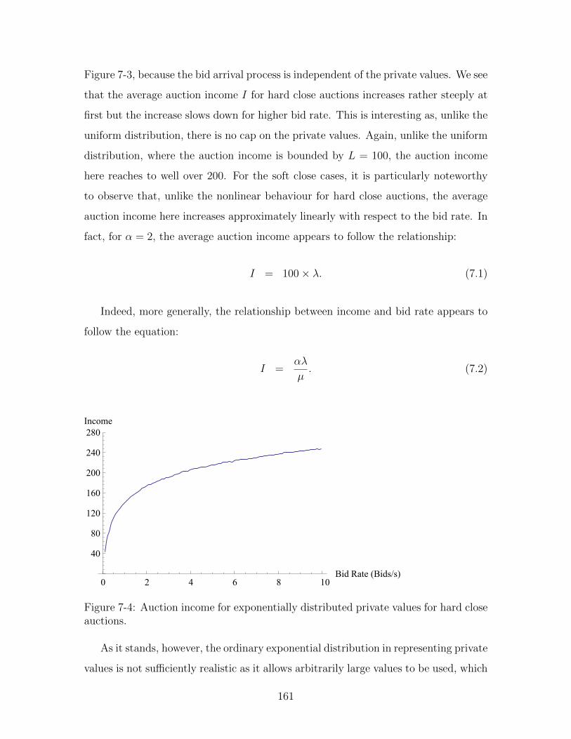
Figure 7-3, because the bid arrival process is independent of the private values. We see

that the average auction income I for hard close auctions increases rather steeply at

first but the increase slows down for higher bid rate. This is interesting as, unlike the

uniform distribution, there is no cap on the private values. Again, unlike the uniform

distribution, where the auction income is bounded by L = 100, the auction income

here reaches to well over 200. For the soft close cases, it is particularly noteworthy

to observe that, unlike the nonlinear behaviour for hard close auctions, the average

auction income here increases approximately linearly with respect to the bid rate. In

fact, for α = 2, the average auction income appears to follow the relationship:

I = 100× λ. (7.1)

Indeed, more generally, the relationship between income and bid rate appears to

follow the equation:

I =αλ

µ. (7.2)


40

80

120

160

200

240

280Income

Figure 7-4: Auction income for exponentially distributed private values for hard closeauctions.

As it stands, however, the ordinary exponential distribution in representing private

values is not sufficiently realistic as it allows arbitrarily large values to be used, which

161

0 0.5 1.0 1.5 2.0 2.5Bid Rate (Bids/s)

60

120

180

240

300

360

420Income

α = 4α = 3α = 2α = 1

Figure 7-5: Auction income for exponentially distributed private values for soft closeauctions.

is often not the case for practical auction processes. For example, for α = 4, the

average highest bid can go up to 400, which is over four times the auction income for

the uniformly distributed private values case, even though both have the same mean

private value. For a more realistic representation of private values, we make use of

the truncated exponential distribution over the same interval as the uniform case,

namely, the interval (0, L), i.e.

f(v) =µe−µv

1− e−µL, for 0 < v < L, (7.3)

and vanishes outside the interval (0, L). Figures 7-6 and 7-7 give the auction

performance for truncated exponentially distributed private values. We see that the

performance behaviour of the ordinary exponential distribution and the truncated

exponential distribution is rather different. However, there is a remarkable similarity

in the auction income behaviour between the truncated exponential private values

and the uniform private values. In the uniform case, the ceiling of 100 is approached

faster than in the truncated exponential case, which as indicated above may be due

to the fact that the bidders in this case is looking for bargains and there is a greater

tendency (probability) to bid for the lower values than the higher ones, whereas in

the uniform case, all the values happen equally likely.

162


20

40

60

80

100

120

140Income

Figure 7-6: Auction income for truncated exponentially distributed private values forhard close auctions.

0 0.5 1.0 1.5 2.0 2.5Bid Rate (Bids/s)

20

40

60

80

100

120

140Income

α = 4α = 3α = 2α = 1

Figure 7-7: Auction income for truncated exponentially distributed private values forsoft close auctions.

7.3 Normally distributed private values

The normal distribution is highly versatile and is representative of a variety of social

and physical phenomena. Here, it represents some measure of implicit agreement

concerning the value of the auction item among the bidder population, since there

is a mode value which they roughly agree upon. In addition, there may even be

some degree of indirect interaction or communication among the global community of

bidders, perhaps through various forms of social networking. Here, we take the mean

163

of the normal distribution η to correspond to the mean of the uniform distribution,

which is L/2 = 50, and likewise we take the variance σ2 to also correspond to the

variance of the uniform distribution, which is L2/12 = 833.33.

Figures 7-8 and 7-9 give the auction performance of the normally distributed pri-

vate values. We see that, while the auction income definitely goes above 100, it is

much more subdued compared with the exponential case for hard close auctions. Sim-

ilar performance behaviour is also evident for soft close auctions. These are probably

due to the strong clustering around the mean/mode. Unlike the exponential case,

however, there is no simple linearity relationship observed, but rather a sub-linear

relationship may be inferred.


20

40

60

80

100

120

140Income

Figure 7-8: Auction income for normally distributed private values for hard closeauctions.

However, the ordinary normal distribution has two properties which limits its

usefulness for auction processes. First, it can go up to +∞, which as indicated earlier

for the exponential distribution, is often not realistic. Second, it can go down to −∞,

which means that negative values are unavoidable no matter how far we shift the

mean to the right, and this again is not permitted in auction processes. As for the

exponential case, we make use of the truncated normal distribution confined to the

164

0 0.5 1.0 1.5 2.0 2.5Bid Rate (Bids/s)

20

40

60

80

100

120

140Income

α = 3α = 2α = 1

α = 4

Figure 7-9: Auction income for normally distributed private values for soft closeauctions.

interval (0, L), i.e.

f(v) =exp

[− (v−η)2

2σ2

]K√

2πσ2, for 0 < v < L, (7.4)

but vanishes outside the interval (0, L), and K is the constant

K =1√

2πσ2

∫ L

0exp

[−(t− η)2

2σ2

]dt. (7.5)

Figures 7-10 and 7-11 give the auction performance for truncated normally dis-

tributed private values. Here, we also see that the performance behaviour of the

ordinary normal distribution and the truncated normal distribution is rather differ-

ent, and there is also a remarkable similarity in the auction income behaviour between

the truncated normal private values and the uniform private values. Similar to the

remarks for the truncated exponential case, in the truncated normal case, the ceiling

of 100 is approached slower than in the uniform case which may be due to the clus-

tering of values around the mean/mode that limits its scope in going up to very high

private values.

We thus see that in the modelling of private values, the uniform distribution as

well as the truncated versions of the normal and exponential distributions are more

165


20

40

60

80

100

120

140Income

Figure 7-10: Auction income for truncated normally distributed private values forhard close auctions.

0 0.5 1.0 1.5 2.0 2.5Bid Rate (Bids/s)

20

40

60

80

100

120

140Income

α = 3α = 2α = 1

α = 4

Figure 7-11: Auction income for truncated normally distributed private values forsoft close auctions.

realistic and versatile. The average auction incomes for these three distributions

exhibit similar behaviour in response to the bid level. It is interesting to compare

how quickly the ceiling of L is approached in these cases. Table 7.1 shows the different

bid rates in attaining 70%, 80%, and 90% of the ceiling L for the hard close auctions.

From the sellers’ point of view, the preferred private values distribution is the uniform,

since it attains a high average income more quickly than the other two distributions.

The least preferred is the truncated exponential distribution since it is the slowest

among the three private values distribution to attain high average income, probably

166

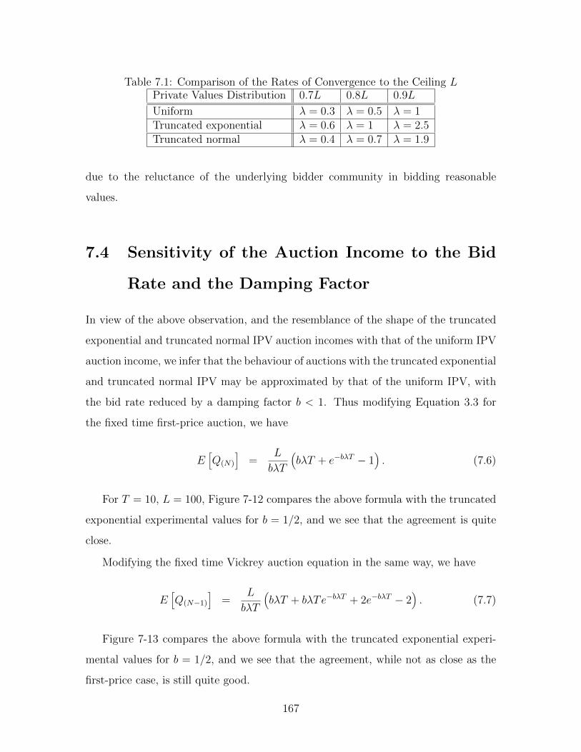
Table 7.1: Comparison of the Rates of Convergence to the Ceiling LPrivate Values Distribution 0.7L 0.8L 0.9L

Uniform λ = 0.3 λ = 0.5 λ = 1Truncated exponential λ = 0.6 λ = 1 λ = 2.5Truncated normal λ = 0.4 λ = 0.7 λ = 1.9

due to the reluctance of the underlying bidder community in bidding reasonable

values.

7.4 Sensitivity of the Auction Income to the Bid

Rate and the Damping Factor

In view of the above observation, and the resemblance of the shape of the truncated

exponential and truncated normal IPV auction incomes with that of the uniform IPV

auction income, we infer that the behaviour of auctions with the truncated exponential

and truncated normal IPV may be approximated by that of the uniform IPV, with

the bid rate reduced by a damping factor b < 1. Thus modifying Equation 3.3 for

the fixed time first-price auction, we have

E[Q(N)

]=

L

bλT

(bλT + e−bλT − 1

). (7.6)

For T = 10, L = 100, Figure 7-12 compares the above formula with the truncated

exponential experimental values for b = 1/2, and we see that the agreement is quite

close.

Modifying the fixed time Vickrey auction equation in the same way, we have

E[Q(N−1)

]=

L

bλT

(bλT + bλTe−bλT + 2e−bλT − 2

). (7.7)

Figure 7-13 compares the above formula with the truncated exponential experi-

mental values for b = 1/2, and we see that the agreement, while not as close as the

first-price case, is still quite good.

167

0 2 4 6 8 10

20

40

60

80

100

Bid Rate

Income

ExperimentalTheoretical

Figure 7-12: Analytic formula for the truncated exponentially distributed IPV forfirst-price auctions.

The damping factor applied to λ represents a fractional reduction in bid traffic,

and hence a damping factor less than one indicates that, compared with the uni-

formly distributed IPV, the corresponding traffic gives a lesser auction income than

the uniformly distributed IPV. The damping factor of b = 1/2 for the truncated

exponential is a significant reduction, and as remarked earlier, it represents bidders

who are looking for bargains and are less generous than those with the corresponding

uniformly distributed private values. Indeed, it is useful to compare the generosity

characteristics of the two distributions. Denoting by Qexp the truncated exponential

IPV bids, and Quniform the uniform IPV bids, we have for v < L,

Pr [Qexp < v] =1− eµv

1− e−µL(7.8)

Pr [Quniform < v] =v

L(7.9)

Since the truncated exponential IPV tend to have bids clustering more at the

lower end compared with the uniform IPV, therefore the relative generosity of the

uniform IPV may be indicated by the probability of a bid exceeding a certain value v

Pr [Qexp > v] < Pr [Quniform > v] , (7.10)

168

which is equivalent to

Pr [Quniform < v] < Pr [Qexp < v] , (7.11)

That is,

1− e−µv

v>

1− e−µv

L. (7.12)

Since L > v, thus condition (Equation 7.10) will be true if we can show that the

function

f(x) =1− e−µv

x. (7.13)

is a decreasing function, i.e. the derivative f ′(x) < 0. Now

f ′(x) =e−µx(1 + µx)− 1

x2. (7.14)

Since (1 + µx)/ exp(µx) < 1, we see that f ′(x) < 0, and so establishing condition

(Equation 7.10), showing that adopting the truncated exponential IPV is more frugal

than the uniform IPV.

As for the truncated normal distribution for the IPV, Figure 7-14 compares Equa-

tion 7.6 with the corresponding truncated normal experimental values for b = 2/3,

and we also see that the agreement is quite close. Also, Figure 7-15 compares Equa-

tion 7.7 with the corresponding truncated normal experimental values for b = 2/3,

and we observe that the agreement, while not as close as the first-price case, seems

quite workable as an approximation.

Thus, we see that both for the truncated exponential and truncated normal IPVs,

the auction income may be usefully approximated by Equations 7.6 and 7.7 respec-

tively for the first-price and Vickrey auctions with appropriate damping factor b. In

both of these cases, the damping factor is less than one, with that for the truncated

exponential distribution smaller than that for the truncated normal distribution. Of

169

0 2 4 6 8 10

20

40

60

80

100

Bid Rate

Income

Experimental

Theoretical

Figure 7-13: Analytic formula for the truncated exponentially distributed IPV forVickrey auctions.

0 2 4 6 8 10

20

40

60

80

100

Bid Rate

Income

Experimental

Theoretical

Figure 7-14: Analytic formula for the truncated normally distributed IPV for first-price auctions.

course, in the case of the uniform distribution, b = 1.

7.5 Summary

We have studied the sensitivity of the auction income to the form of the IPV distribu-

tions. To be realistic, we focus attention on those admitting a finite range of positive

170

0 2 4 6 8 10

20

40

60

80

100

Bid Rate

Income

Experimental

Theoretical

Figure 7-15: Analytic formula for the truncated normally distributed IPV for Vickreyauctions.

values, which include the uniform, truncated normal, and truncated exponential dis-

tributions. The uniform distribution may be used to represent bidders of whose IPV

very little is known, with all values within the range occurring with equal probability.

On the other hand, the truncated normal distribution may be used to represent the

community of bidders in which there is some degree of agreement on the value of

the item being auctioned. Since consumers are often looking for bargains in Internet

auctions (as opposed to obtaining the good through conventional channels), many

tend to bid at the lower end of the spectrum of values, and such social behaviour

may be represented by the truncated exponential IPV distribution, where the lower

value clusters have a greater probability of occurring. For these distributions, we have

found that their performances exhibit a remarkable similarity in their pattern of in-

crease. In all such IPV distributions, the average auction income tends to rise rather

steeply at first and then gradually settles to approach the ceiling value. Using the

damping factor which suitably reduces the bid rate, analytic formulae are obtained

for the auction incomes for auctions which adopt the truncated exponential IPV and

truncate normal IPV. We have found that the uniform IPV is the most generous with

a damping factor of one. The truncated normal IPV is more frugal than the uniform

IPV with a smaller damping factor, while the most frugal of the three is the truncated

171

exponential IPV which has the smallest damping factor compared with the other IPV

distributions.

172

Chapter 8

Conclusions and Future Work

8.1 Summary of Achievements

The present study provides the first systems model of Internet Auction Processes. It

is able to give good prediction of Internet auction performance, and the closed-form

analytic results are able to furnish fairly good agreements with observed measure-

ments.

The value of such model may be usefully compared with those of Queueing Sys-

tems. While actual queueing systems in general admit considerable complexity such

as transient behaviour, inter-dependent arrivals, rush hour characteristics, corre-

lated service times, diverse scheduling rules etc., tractable and manageable system

model such as the M/G/1 steady state queue (along with the well-known Pollazcek-

Khintchine formula) nevertheless provides useful quantitative results as well as valu-

able insights and approximations into the performance and behavioural characteris-

tics of queueing systems, even though the M/G/1 queue is recognised to be a gross

simplification of reality. Similar to Kendall’s notation for queueing systems, we can

characterise Internet Auction Processes in terms of a set of properties.

The first is the arrival characteristics; e.g. as in queueing theory, we may use M to

denote homogeneous Poisson (Markov) arrival, and M(t) to denote non-homogeneous

Poisson arrival.

The second is the distribution of the private values; e.g. we may use U to signify

173

that the values are uniformly distributed, N to signify that the values are normally

distributed, and M to signify that the values are exponentially distributed. Since pri-

vate values are bounded, it is often more realistic to use the corresponding truncated

distributions for N and M . Therefore the corresponding truncated distribution is

assumed to be used whenever we indicate N or M .

The third is the relative ranking of the accepted bid; e.g. we may use FP to denote

first-price auctions, V K to denote Vickrey auctions, and LP to denote lowest price

auctions.

The fourth is the intended auction duration; e.g. we may use FT to denote fixed-

time auctions, and V T to denote variable-time auctions.

The fifth is whether there is the option of early termination of an auction, e.g. on

receiving a sufficiently high bid (such as Buy-It-Now or BIN) or a sufficiently low bid

(Sell-It-Now or SIN); when such early termination option is not available, then we

would simply omit this specification, meaning that the auction will always be allowed

to run its normal course to completion. In the case where the auction is designed to

terminate on receiving a pre-specified number of bids k, then we would simply use k

to indicate this in the fifth component.

For example, a first-price auction with Poisson arrival, uniformly distributed pri-

vate values, which uses a fixed auction duration but allows early termination at the

point when a sufficiently large bid is received is denoted by M/U/FP/FT/BIN .

A comparison between some of the attributes of Internet Auction Systems and

Queueing Systems is useful (see Table 8.1).

Internet Auction Systems Queueing Systems

Independent Values Distribution Service Time DistributionPrice Selection Criterion (e.g. First-Price) Customer Selection Criterion (e.g. FCFS)Number of Bids Accepted Number of ServersAuction Duration (exceeding which no bidis allowed)

Waiting Room Capacity (exceeding whichno customer is allowed)

Premature Auction Termination Service PreemptionBid Arrival Pattern Customer Arrival Pattern

Table 8.1: Comparison Between Internet Auction Systems and Queueing Systems.

174

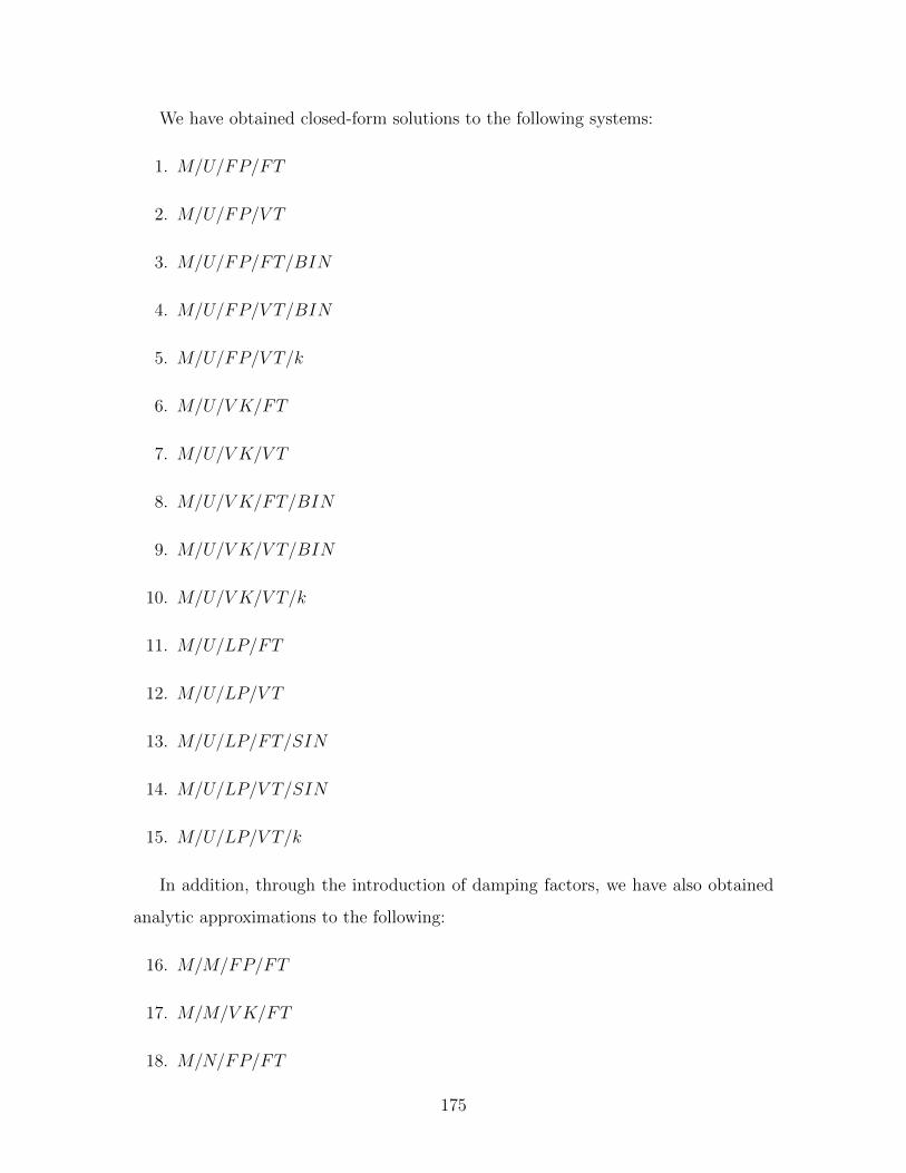
We have obtained closed-form solutions to the following systems:

1. M/U/FP/FT

2. M/U/FP/V T

3. M/U/FP/FT/BIN

4. M/U/FP/V T/BIN

5. M/U/FP/V T/k

6. M/U/V K/FT

7. M/U/V K/V T

8. M/U/V K/FT/BIN

9. M/U/V K/V T/BIN

10. M/U/V K/V T/k

11. M/U/LP/FT

12. M/U/LP/V T

13. M/U/LP/FT/SIN

14. M/U/LP/V T/SIN

15. M/U/LP/V T/k

In addition, through the introduction of damping factors, we have also obtained

analytic approximations to the following:

16. M/M/FP/FT

17. M/M/VK/FT

18. M/N/FP/FT

175

19. M/N/V K/FT

Moreover, through appropriately transforming the timescale, we have been able

to generalise most of the above results from a homogeneous Poisson arrival pattern

of M to a non-homogeneous arrival pattern of M(t), which is able to model a wide

variety of bid arrival characteristics in a versatile manner.

8.2 Optimal Auction Scenarios

From this thesis, I have learned auctions algorithms on the Internet have room for

incorporating greater complexity. Some of the algorithms studied here are more

complex than the existing Internet algorithms (e.g. Algorithms 3.3 and 3.4), and if

users are willing to accept such complexity, these can be incorporated into Internet

auctions.

The optimal auction scenario from the point-of-view of the seller is to run a fixed-

time Vickrey auction, since Vickrey auctions encourage bidder participation, and

consequently higher bid rates translate to higher incomes. Additionally, a high bid

rate will narrow the price difference between the first-price and second price anyway.

Choosing a fixed-time auction makes it easier to manage and as the seller, I can be

assured of getting the money by a specific time rather than having to wait for a period

of uncertain length in the case of a soft-close auction. The length of the auction will

be so chosen that the expected income is higher than my target surplus.

The optimal auction scenario from the point-of-view of the buyer is to participate

in an auction with Open BIN (either hard-close or soft-close) where M is lower than

the price I am willing to pay. Doing so will mean that I can get the resource quickly

without having to wait for the auction to finish. If such an auction is not available,

I would choose a Vickrey auction, where I get the assurance that I won’t overpay

compared with other bidders.

176

8.3 Future Work

As for queueing systems, the varieties and types of Internet Auction processes admit

wide variations, and the characteristics and performance of different such auction

systems will clearly be worthy of further study. In future, some of the components of

Internet Auction Systems may be extended to characterise different auction situations

and algorithms. Unlike conventional auctions, arbitrarily complex auction algorithms

may be designed and adopted for Internet Auctions.

While the probability distributional assumptions that we use have been commonly

adopted in other studies, it will be useful in particular to extend the Independent

Private Values characteristics to other distributions for modelling the behaviour of

different types of bidding communities. For example, it will be interesting to gen-

eralise the above results to such widely-used distributions as the Erlang distribution

and the Pareto distribution.

Indeed, any one of the five components of an Internet auction system may be

usefully generalised and extended. Admittedly, however, exact results may not be

easy to obtain, and approximations would have to be used. Such approximations may

relate to the adoption of assumptions that are close but not completely matching the

particular situations, or approximations that are related to the mathematical analysis

of the model or both. Such approximate expressions, even though do not give a full

and complete correspondence with the underlying reality, will nevertheless be able

to provide useful insight into the operation of Internet auction processes and furnish

mechanisms for the practical optimisation of the relevant auction parameters.

Since Internet auctions is becoming prevalent and ubiquitous, with significant

parts of the commodities and resources markets based on auctions rather than the

fixed-price model, the systematic quantitative study of Internet auction models will be

increasingly useful and essential to impart a deeper understanding of the performance

behaviour of such processes and mechanisms.

177

Appendix A

eBay Auction Data

179

Table A.1: Auction of “Apple iPhone 4 16GB- BLACK- UNLOCKED JAILBRO-KEN, NEW!!!” to “ ***n” for USD575.00.

Bid Date Bid Time Bidder Private Value Time Between Bids (s)

7/13/2011 18:207/13/2011 18:07 ***n 575.007/13/2011 02:29 h***h 565.00 562687/12/2011 21:53 k***e 540.00 165597/12/2011 18:40 i***r 450.00 116027/12/2011 13:42 i***i 300.00 178677/12/2011 06:01 a***a 265.00 276497/12/2011 03:23 0***9 250.50 94657/11/2011 14:03 e***2 230.00 480217/11/2011 07:45 o***p 220.00 226517/11/2011 03:45 y***a 220.00 144397/11/2011 00:17 i***k 200.00 124517/11/2011 00:12 d***n 110.00 3107/10/2011 20:28 r***y 75.00 134457/10/2011 20:09 m***s 50.00 11447/10/2011 18:55 l***t 189.23 44217/10/2011 18:45 n***c 3.00 6357/10/2011 18:20 1468

180

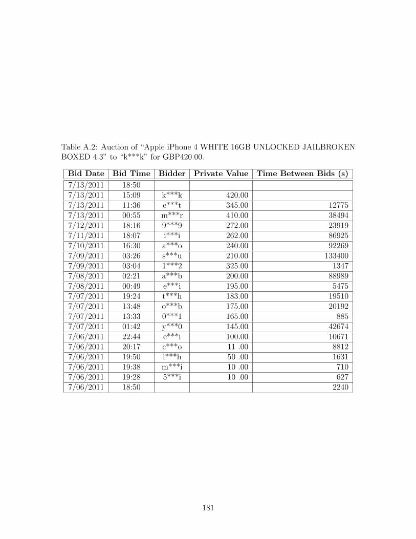
Table A.2: Auction of “Apple iPhone 4 WHITE 16GB UNLOCKED JAILBROKENBOXED 4.3” to “k***k” for GBP420.00.


7/13/2011 18:507/13/2011 15:09 k***k 420.007/13/2011 11:36 e***t 345.00 127757/13/2011 00:55 m***r 410.00 384947/12/2011 18:16 9***9 272.00 239197/11/2011 18:07 i***i 262.00 869257/10/2011 16:30 a***o 240.00 922697/09/2011 03:26 s***u 210.00 1334007/09/2011 03:04 1***2 325.00 13477/08/2011 02:21 a***b 200.00 889897/08/2011 00:49 e***i 195.00 54757/07/2011 19:24 t***h 183.00 195107/07/2011 13:48 o***b 175.00 201927/07/2011 13:33 0***1 165.00 8857/07/2011 01:42 y***0 145.00 426747/06/2011 22:44 e***i 100.00 106717/06/2011 20:17 c***o 11 .00 88127/06/2011 19:50 i***h 50 .00 16317/06/2011 19:38 m***i 10 .00 7107/06/2011 19:28 5***i 10 .00 6277/06/2011 18:50 2240

181

Table A.3: Auction of “NEW! iPhone 4 16GB black JAILBROKEN!!! + FREEAPPS” to “a***a” for USD475.00.


7/13/2011 20:007/13/2011 20:00 a***a 475.007/13/2011 18:39 0***8 470.00 48507/13/2011 18:21 o***i 417.00 10937/13/2011 17:15 i***i 430.00 39437/13/2011 15:09 m***r 355.00 75457/13/2011 07:45 a***s 350.00 266687/13/2011 02:47 e***s 310.00 178717/12/2011 18:15 s***i 220.00 307297/12/2011 16:59 k***n 210.00 45397/12/2011 13:30 y***r 185.00 125317/12/2011 01:34 a***1 180.00 429677/11/2011 04:06 h***m 120.00 773087/10/2011 10:24 s***n 115.00 637007/10/2011 05:37 i***9 100.00 172157/10/2011 01:07 n***v 100.00 162087/09/2011 06:14 s***i 25 .00 679537/09/2011 00:37 p***n 75 .00 202227/08/2011 20:00 16655

182

Table A.4: Auction of “Apple iPhone 4 16GB new” to “c***o” for USD540.00.


7/13/2011 20:387/13/2011 18:31 c***o 540.007/13/2011 15:53 b***a 500.00 95037/13/2011 13:25 u***1 450.00 88827/13/2011 10:58 i***k 530.00 88187/13/2011 08:59 i***n 410.00 71307/13/2011 08:41 n***e 405.00 10667/13/2011 07:59 1***a 380.00 25007/13/2011 07:26 n***d 360.00 19977/13/2011 07:09 a***a 400.00 10527/13/2011 07:07 t***i 300.00 817/13/2011 06:23 l***a 350.00 26497/13/2011 05:30 i***r 255.00 31697/13/2011 05:11 d***o 240.00 11287/13/2011 05:02 0***r 250.00 5827/13/2011 04:06 0***e 200.00 33237/13/2011 03:22 3***e 192.00 26367/13/2011 03:08 n***6 90 .00 8807/13/2011 03:02 r***n 170.00 3357/13/2011 03:00 n***c 45 .00 1537/13/2011 02:54 z***n 40.00 3357/13/2011 02:53 r***x 20.00 727/12/2011 20:38 22490

183

Table A.5: Auction of “Apple iPhone 4 (Latest Model) - 16GB - White (AT&T)NEW” to “a***d” for USD525.00.


7/14/2011 03:057/14/2011 03:05 a***d 525.007/14/2011 03:04 p***p 515.00 277/13/2011 22:29 j***m 496.00 165057/13/2011 18:56 i***i 485.01 128157/13/2011 17:44 a***c 350.00 43107/13/2011 14:40 s***f 320.00 110117/13/2011 13:22 a***m 450.00 47167/13/2011 07:37 g***1 290.00 206777/13/2011 04:24 k***a 260.00 115957/13/2011 04:17 e***e 300.99 4267/13/2011 04:16 h***h 250.00 627/13/2011 03:51 y***e 70 .00 15107/13/2011 03:34 i***h 50 .00 10107/13/2011 03:14 8***m 27 .00 11587/13/2011 03:12 l***d 26 .00 1187/13/2011 03:05 460

184

Appendix B

Generalisation to

Non-Homogeneous Poisson Process

While many previous studies modelled the bid arrival process as a Poisson process

with constant arrival rate λ, a more versatile model will be to allow λ to be a function

of time, i.e.

Pr[an arrival occurring in (t, t+ ∆t)] ≈ λ(t)∆t. (B.1)

In such a process, the number of bid arrivals in the time interval (t, t + ∆t) is

still independent of what happens in other time intervals. This process is known

by various names such as non-homogeneous Poisson process, non-stationary Poisson

process, time-dependent Poisson process, and in our study, the term non-homogeneous

Poisson process will be used. To generalise on the results of Chapter 3, we need to

replace the number of bids N by N(t), which signifies the number of bids arrived in

the time interval (0, t), and denoting by R(t), the following integral

R(t) =∫ t

0λ(x)dx,

185

from Mieghem (2006), we have the non-homogeneous Poisson distribution

Pr[N(t) = k] =e−R(t)R(t)k

k!, (B.2)

the mean value of which is given by R(t).

B.1 Algorithm I: Fixed Time Forward Auction

To determine the average income E[QN(T )] for the present situation, we remove the

condition on N(t) in Equation 3.1 using the probabilities in Equation B.2 with t = T ;

i.e.

E[QN(T )

]=

∞∑N(T )=1

N(T )L

N(T ) + 1× e−R(T )R(T )N(T )

N(T )!

=∞∑

N(T )=1

[L− L

N(T ) + 1

]× e−R(T )R(T )N(T )

N(T )!

=∞∑

N(T )=1

L× e−R(T )R(T )N(T )

N(T )!−

∞∑N(T )=1

L

N(T ) + 1× e−R(T )R(T )N(T )

N(T )!

= L(1− e−R(T )

)− Le−R(T )

R(T )

∞∑N(T )=1

R(T )N(T )+1

(N(T ) + 1)!

= L(1− e−R(T )

)− Le−R(T )

R(T )

(eR(T ) − 1−R(T )

)

which simplifies to

E[QN(T )

]=

L

R(T )

(R(T ) + e−R(T ) − 1

),

i.e.

E[QN(T )

]=

L(∫ T

0 λ(x)dx)

+[exp

(−∫ T

0 λ(x)dx)]− 1

∫ T

0 λ(x)dx, (B.3)

Fixed time auctions are particularly susceptible to sniping where the closing time

186

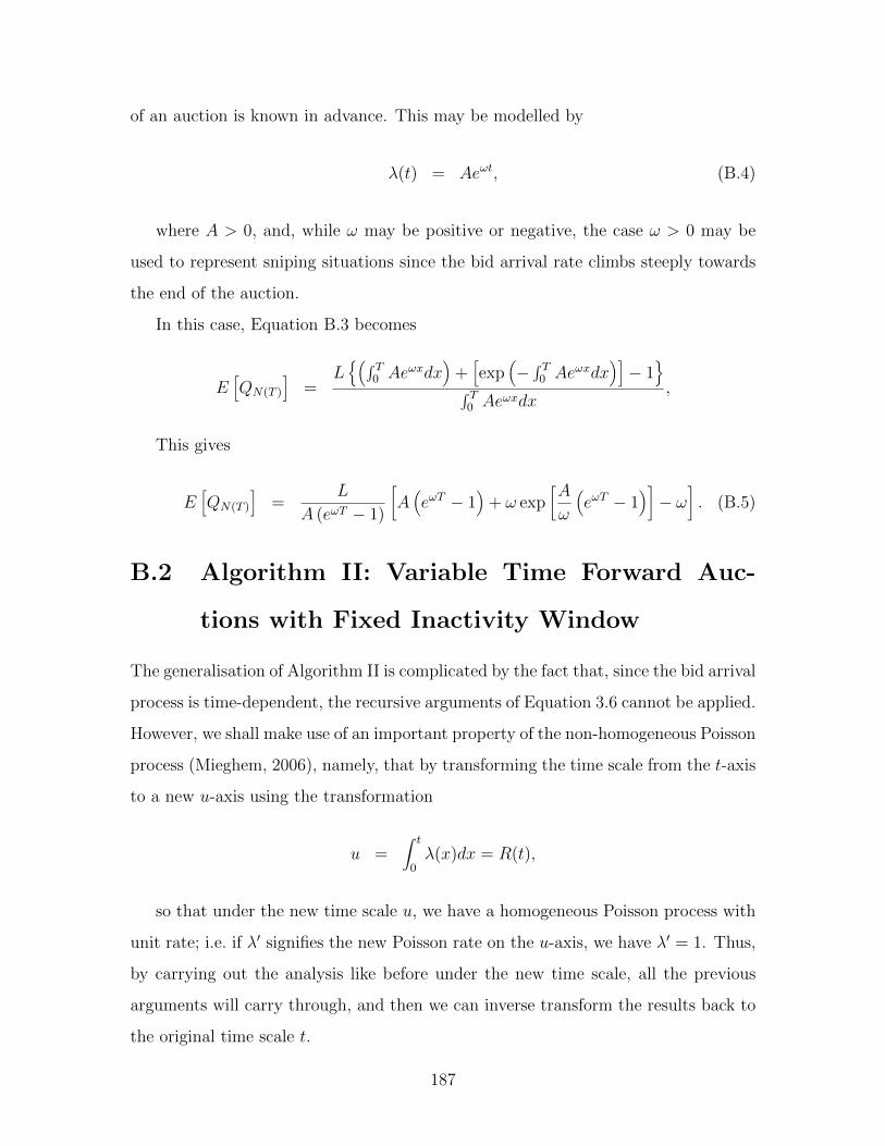
of an auction is known in advance. This may be modelled by

λ(t) = Aeωt, (B.4)

where A > 0, and, while ω may be positive or negative, the case ω > 0 may be

used to represent sniping situations since the bid arrival rate climbs steeply towards

the end of the auction.

In this case, Equation B.3 becomes

E[QN(T )

]=

L(∫ T

0 Aeωxdx)

+[exp

(−∫ T

0 Aeωxdx)]− 1

∫ T

0 Aeωxdx,

This gives

E[QN(T )

]=

L

A (eωT − 1)

[A(eωT − 1

)+ ω exp

[A

ω

(eωT − 1

)]− ω

]. (B.5)

B.2 Algorithm II: Variable Time Forward Auc-

tions with Fixed Inactivity Window

The generalisation of Algorithm II is complicated by the fact that, since the bid arrival

process is time-dependent, the recursive arguments of Equation 3.6 cannot be applied.

However, we shall make use of an important property of the non-homogeneous Poisson

process (Mieghem, 2006), namely, that by transforming the time scale from the t-axis

to a new u-axis using the transformation

u =∫ t

0λ(x)dx = R(t),

so that under the new time scale u, we have a homogeneous Poisson process with

unit rate; i.e. if λ′ signifies the new Poisson rate on the u-axis, we have λ′ = 1. Thus,

by carrying out the analysis like before under the new time scale, all the previous

arguments will carry through, and then we can inverse transform the results back to

the original time scale t.

187

Under the transformed time scale, the parameter α will become α′, with

α′ =∫ α

0λ(x)dx = R(α), (B.6)

and under this transformed time scale, the auction duration from Equation 3.7,

bearing in mind that the rate of the process is now unity, is

τ ′α′ = eα′ − 1 = eR(α) − 1. (B.7)

Hence, the required auction duration τα satisfies

R(τα) = eR(α) − 1. (B.8)

Or in terms of the inverse function

τα = R−1[eR(α) − 1

]. (B.9)

From Equation B.8 we may determine τα from the following equation

∫ τα

0λ(x)dx = exp

(∫ α

0λ(x)dx

)− 1. (B.10)

which, in general, may be solved by numerical methods. For certain simple cases,

closed form solutions may be obtained. For example, in the simple case λ(t) = bt,

then we have from Equation B.10

bτ 2α

2= e

ba2

2 − 1.

giving

τα =

√√√√2eba2

2 − 2

b.

Here, we have λ(0) = 0, which may sometimes be restrictive. For a more general

188

linear form λ(t) = a + bt, the solution to τα is more complicated but still admits a

closed-form solution. Here, we have

R(τα) =∫ τα

0(a+ bx)dx = aτα +

bτ 2α

2.

To determine the inverse function R−1, we let y = R(τα), and solve for τα in terms

of y. That is,

y = ατα +bτ 2α

2,

which gives

bτ 2α + 2ατα − 2y = 0.

Solving this using the quadratic formula, we have

τα =−2a±

√4a2 + 8by

2b.

Taking the positive square root and simplifying, we have

τα =−a+

√a2 + 2by

b.

That is,

R−1(y) =−a+

√a2 + 2by

b.

From Equation B.9, we have

τα = R−1[eR(α) − 1

]=−a+

√a2 + 2b [eR(α) − 1]

b.

189

That is, we obtain

τα = R−1[eR(α) − 1

]=−a+

√a2 + 2b [eaα+bα2/2 − 1]

b. (B.11)

It is useful to note that as b → 0, λ → a, the limit of the right hand side of

Equation B.11 tends to (eaα − 1) /a, which can be seen by application of L’Hopital’s

rule, and this result is in agreement with Equation 3.7.

For

λ(t) = Aeωt,

from B.10, we have

∫ τα

0Aeωxdx = exp

(∫ α

0Aeωxdx

)− 1, (B.12)

i.e.

Aeωτα

ω=

[exp

(∫ α

0

Aeωα

ω

)]− 1 +

A

ω

or

eωτα =ω

A

[exp

(A

ω(eωα − 1)

)]− ω

A+ 1

giving

τα =1

ωloge

(ω

A

[exp

(A

ω(eωα − 1)

)]− ω

A+ 1

).

We also note that as ω → 0, λ → A, and τα tends to(eAα − 1

)/A, which can

be seen most readily from Equation B.12, and this result is in agreement with Equa-

tion 3.7.

Since bidding sometimes takes place more frequently at certain times of day but

less so at other times, a periodic λ(t) may be usefully employed to model this situation;

190

here we may take

λ(t) = A1 cos(ωt− φ) + A0. (B.13)

From B.10, we have

∫ τα

0(A1 cos(ωx− φ) + A0) dx = exp

(∫ α

0(A1 cos(ωx− φ) + A0) dx

)− 1,

i.e.

A1 (sin (ωτα − φ) + sinφ)

ω+ A0τα = e(A1/ω)(sin(ωα−φ)+sinφ)+A0α − 1,

from which τα may be solved numerically. In the special case φ = 0, the above

simplifies to

A1 sinωταω

+ A0τα = e(A1 sinωα/ω)+A0α − 1, (B.14)

For example, if A0 = 2, A1 = 1, ω = 1, and α = π, Equation B.14 becomes

2τα + sin τα = e2π − 1

Solving for τα numerically gives τα = 267.5. It is interesting to note that when

A1 = 0, then λ(t) = A0 and Equation B.14 becomes

A0τα = eA0α − 1,

which is in agreement with Equation 3.7.

In general, the inverse function would be difficult to obtain, but if λ(t) is a mono-

tonic function, then useful bounds may be obtained. For example, if λ(t) is mono-

tonically increasing with λ(0) ≤ λ(t), then since we know from previous analysis of

Algorithm II that the auction duration is an increasing function of λ, thus the auction

191

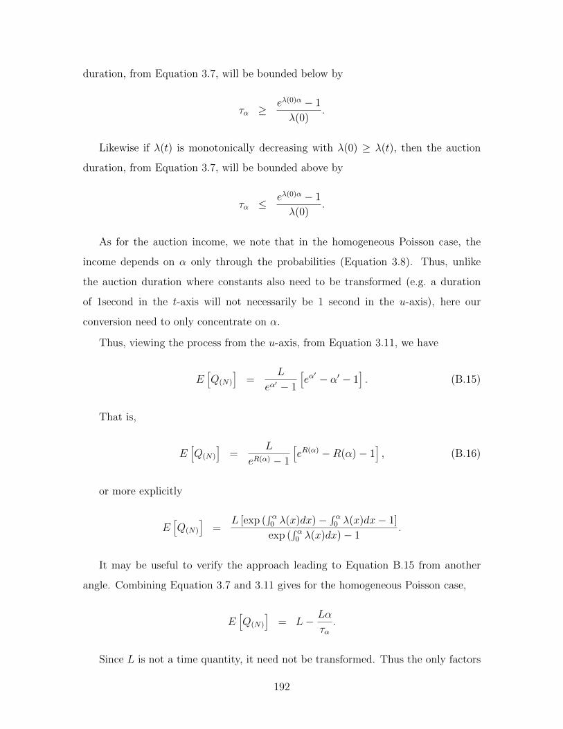
duration, from Equation 3.7, will be bounded below by

τα ≥eλ(0)α − 1

λ(0).

Likewise if λ(t) is monotonically decreasing with λ(0) ≥ λ(t), then the auction

duration, from Equation 3.7, will be bounded above by

τα ≤eλ(0)α − 1

λ(0).

As for the auction income, we note that in the homogeneous Poisson case, the

income depends on α only through the probabilities (Equation 3.8). Thus, unlike

the auction duration where constants also need to be transformed (e.g. a duration

of 1second in the t-axis will not necessarily be 1 second in the u-axis), here our

conversion need to only concentrate on α.

Thus, viewing the process from the u-axis, from Equation 3.11, we have

E[Q(N)

]=

L

eα′ − 1

[eα′ − α′ − 1

]. (B.15)

That is,

E[Q(N)

]=

L

eR(α) − 1

[eR(α) −R(α)− 1

], (B.16)

or more explicitly

E[Q(N)

]=

L [exp (∫ α

0 λ(x)dx)−∫ α

0 λ(x)dx− 1]

exp (∫ α

0 λ(x)dx)− 1.

It may be useful to verify the approach leading to Equation B.15 from another

angle. Combining Equation 3.7 and 3.11 gives for the homogeneous Poisson case,

E[Q(N)

]= L− Lα

τα.

Since L is not a time quantity, it need not be transformed. Thus the only factors

192

that need to be transformed here are α and τα, giving for the non-homogeneous

Poisson case

E[Q(N)

]= L− Lα′

τ ′α′.

From Equations B.6 and B.7 this gives

E[Q(N)

]= L− LR(α)

eR(α) − 1= L

[1− R(α)

eR(α) − 1

].

which again yields Equation B.16. This indicates that the above approach that

concentrates only on the conversion of α and the arrival rate will yield correct results.

That is, since the income is measured in monetary terms, it should be the same irre-

spective of which time scale is used, and consequently only time-related parameters,

such as the length of the inactivity window and the arrival rate, need to be adjusted.

In the case when λ(t) = a+ bt, we have

E[Q(N)

]=

L[eaα+bα2/2 − aα− bα2/2− 1

]e(aα+bα2/2) − 1

We see that as b→ 0, λ→ α, and the above tends to

E[Q(N)

]=

L

eaα − 1[eaα − aα− 1] ,

which is in agreement with Equation 3.11. In the case when λ(t) is given by

Equation B.4, we have

E[Q(N)

]=

L [exp (∫ α

0 Aeωxdx)−

∫ α0 Ae

ωxdx− 1]∫ α0 Ae

ωxdx− 1

=ωL× exp

[Aω

(eωα − 1)− Aω

(eωα − 1)− 1]

A (eωα − 1).

We see that as ω → 0, λ→ A, and the above tends to

E[Q(N)

]=

L

eAα − 1

[eAα − Aα− 1

],

193

which is in agreement with Equation 3.11. In the case when λ(t) is periodic as

given by Equation B.13, we have from Equation B.16

E[Q(N)

]=

Le(A1/ω)[sin(ωα−φ)+sinφ]+A0α − (A1/ω) [sin(ωα− φ) + sinφ]− A0α− 1

e(A1/ω)[sin(ωα−φ)+sinφ]+A0α − 1

We see that as A1 = 0, then λ = A0, and the above tends to

E[Q(N)

]=

L

eA0α − 1

[eA0α − A0α− 1

],

which, again, is in agreement with Equation 3.11.

B.3 Algorithm III: Fixed Time Forward Auctions

with Fixed Inactivity Window and Maximum

Threshold Termination

Consider the Poisson stream. From (Van Micghem, 2006), the probability density

function of the inter-arrival time f(t) of this stream is

f(t) = Λ(t) exp(−∫ t

0Λ(x)dx

)= pλ(t)e−pR(t). (B.17)

The average auction duration by combining the averages of (i) having an arrival

from Λ(t) in the interval (0, T ), and (ii) having no arrival from Λ(t) in the interval

(0, T ), and making use of Equation B.2 for the Λ(t) stream, is

E [TM ] =∫ T

0tf(t)dt+ T exp

(−∫ T

0Λ(x)dx

). (B.18)

That is,

E [TM ] = p∫ T

0tλ(t)e−pR(t)dt+ Te−pR(T ). (B.19)

As for the auction income, we consider the process on the u-axis, so that from

194

Equation 3.15, and noting that Λ(t) becomes p on the u-axis (since λ(t) is transformed

to unit arrival rate),

E [QM ] =(M + L)

(1− e−pT ′

)2

+Me−pT

′

(1− p)T ′((1− p)T ′ + e−(1−p)T ′ − 1

).(B.20)

Since T ′ = R(T ), this becomes

E [QM ] =(M + L)

(1− e−pR(T )

)2

+Me−pR(T )

(1− p)R(T )

((1− p)R(T ) + e−(1−p)R(T ) − 1

).(B.21)

B.4 Algorithm IV: Variable Time Forward Auc-

tions with Fixed Inactivity Window and Max-

imum Threshold Termination

From Chapter 3, and carrying out the above time transformation, we have for the

average auction duration in the t-axis

E [τM ] = R−1

1− e−α′

p+ p′e−α′

. (B.22)

For the average auction income we have, following the same arguments as in

Chapter 3,

E [Q′M ] =1

p1 + p2

p1M

[1− p′α′

ep′α′ − 1

]+p2(M + L)

2

. (B.23)

B.5 Algorithm V: Auctions on Attaining a Given

Number of Bids

As indicated in Equation B.2, the mean number of bids for the non-homogeneous

Poisson process is given by R(t). Thus the average time τB required to attain B bids

195

is given by

R (τB) =∫ τB

0λ(x)dx = B. (B.24)

Thus,

τB = R−1(B). (B.25)

For λ(t) = a+ bt, we have

R (τB) =∫ τB

0(a+ bx)dx = aτB +

bτ 2B

2= B. (B.26)

This gives

τB =−a+

√a2 + 2bB

b(B.27)

If b → 0, λ(t) → a, and the above tends to B/a, which is in agreement with the

homogeneous Poisson case.

For

λ(t) = Aeωt (B.28)

we have

∫ τB

0Aeωxdx =

AeωτB

ω− A

ω= B, (B.29)

which gives

τB =1

ωloge

(ωB

A+ 1

). (B.30)

Since the number of bids is the same, the auction income for this case is the same

as for the corresponding homogeneous Poisson case.

196

B.6 Algorithm VI: Fixed Time Vickrey Auctions

To determine the average income E[Q(N(T ))−1

]for the present situation, we remove

the condition on N(t) in Equation 3.8 using the probabilities given in Equation B.2

with t = T ; i.e.

E[Q(N(T ))−1

]=

∞∑N(T )=1

(N(T )− 1)L

N(T ) + 1× e−R(T )R(T )N(T )

N(T )!

=∞∑

N(T )=1

[L− 2L

N(T ) + 1

]× e−R(T )R(T )N(T )

N(T )!

=∞∑

N(T )=1

L× e−R(T )R(T )N(T )

N(T )!−

∞∑N(T )=1

2L

N(T ) + 1× e−R(T )R(T )N(T )

N(T )!

= L(1− e−R(T )

)− 2Le−R(T )

R(T )

∞∑N(T )=1

R(T )N(T )+1

(N(T ) + 1)!

= L(1− e−R(T )

)− 2Le−R(T )

R(T )

(eR(T ) − 1−R(T )

)

which simplifies to

E[Q(N(T ))−1

]=

L

R(T )

(R(T ) +R(T )e−R(T ) + 2e−R(T ) − 2

), (B.31)

i.e.

E[Q(N(T ))−1

]=

L(∫ T

0 λ(x)dx+[∫ T

0 λ(x)dx× exp(−∫ T

0 λ(x)dx)]

+[2 exp

(−∫ T

0 λ(x)dx)]− 2

)∫ T

0 λ(x)dx.(B.32)

B.7 Algorithm VII: Variable Time Vickrey Auc-


The average auction duration is given in Section B.2. For the determination of average

auction income, as before, we carry out the time transformation in Equation B.6 so

that the parameter α in the t-axis will become α′ in the u-axis, and from Equation 4.6,

197

we have

E[Q(N(T )−1)

]=

2L

eα′ − 1[sinhα′ − α′] , (B.33)

i.e.

E[Q(N(T )−1)

]=

2L

eR(α) − 1[sinhR(α)−R(α)] . (B.34)

This gives

E[Q(N(T )−1)

]=

2L [sinh∫ α

0 λ(x)dx−∫ α

0 λ(x)dx]

e∫ α

0λ(x)dx − 1

. (B.35)

B.8 Algorithm VIII: Fixed Time Vickrey Auctions

with Maximum Threshold Termination

The average auction duration is given in Section B.3. For the determination of average

auction income, as before, we carry out the time transformation in Equation B.6 and

using the unit arrival rate in the u-axis, we have from Equation 4.9,

E [QMv] =(M + L)

(1− e−pT ′

)2

+Me−pT

′

p′T ′

(p′T ′ + p′T ′e−p

′T ′ + 2e−p′T ′ − 2

),(B.36)

where

T ′ =∫ T

0λ(x)dx. (B.37)

198

B.9 Algorithm IX: Variable Time Vickrey Auc-

tions with Fixed Inactivity Window and Max-


Here, we carry out the same transformation, and following similar arguments as

previously, we have for the average auction income,

E [Q′M ] =1

p1 + p2

[p1 (sinh (p′α′) + p′α′) + p2

M + L

2

]. (B.38)

The average auction duration here is the same as that given in Algorithm IV.

B.10 Algorithm X: Vickrey Auctions on Attaining

a Given Number of Bids

Here, the average magnitude of the accepted bid is given by Equation 4.13, while the

average auction duration is given by Equation B.25.

B.11 Algorithm XI: Fixed Time Reverse Auctions

Here, the auction duration is fixed and equals T . Following the techniques of previous

analysis, we have, for the average auction income

E[Q(1)

]=

∞∑N=0

L

N(T ) + 1× e−R(T )R(T )N(T )

N(T )!

=Le−R(T )

R(T )

(eR(T ) − 1

).

That is,

E[Q(1)

]=

L

R(T )

(1− e−R(T )

)(B.39)

199

B.12 Algorithm XII: Variable Time Reverse Auc-


Similar to previous approach, from Chapter 4, we have for the auction income

E[Q(1)

]=

LR(α)

eR(α) − 1. (B.40)

The average auction duration is similar to that obtained for Algorithm II.

B.13 Algorithm XIII: Fixed Time Reverse Auc-

tions with Minimum Threshold Termination

The average auction duration is similar to that obtained for Algorithm III. Carrying

out the same transformation as before, the average magnitude of the accepted bid

E [Qm], from Chapter 4, is

E [Qm] = L−

(2L−m)(1− e−pT ′

)2

+(L−m)e−pT

′

p′T ′

[p′T ′ + e−p

′T ′ − 1] .(B.41)

B.14 Algorithm XIV: Variable Time Reverse Auc-

tions with Fixed Inactivity Window and Min-


Following the same approach as previously, the average magnitude of the accepted

bid E [Qm] is, from Chapter 4,

E [Qm] = L−

e−α′[(L−m)

(1− p′α′

e−p′α′−1

)]+ 2L−m

2

(1− e−pα′

) (p+ p′e−α

′)

e−α′ + (1− e−pα′) (p+ p′e−α′)

.(B.42)

where p = mL

. The average auction duration is similar to that obtained for Algo-

rithm IV.

200

B.15 Algorithm XV: Reverse Auctions on Attain-

ing a Given Number of Bids

Here, as before, the average auction duration required to attain B bids is the same

as Algorithm V, while the auction income is the same as for the corresponding non-

homogeneous Poisson case.

B.16 Empirical Representation of eBay arrivals us-

ing Non-Homogeneous Poisson Process

From the eBay auction data in Appendix A, some degree of non?uniformity seems to

exist in the bid arrival pattern within individual auctions. Thus, the non?homogeneous

?Poisson process may be usefully employed to represent some of these situations.

?For example, for Auction A2, we can represent the arrival pattern as (using day

as the ?time unit and counting the number of bid arrivals in each 24?hour period):

?λ(1) = 8;λ(2) = 3?;λ(3) = 2;λ?(4) = 1;λ?(5) = 1;λ?(6) = 1;λ?(7) = 4,? the rates

of which show considerable variation and range from 1 to 8. Also, for Auction ?A3, we

can represent the arrival pattern as λ(1) = 2;λ(2) = 3;λ(3) = 1;λ(4) = 4;λ(5) = 8,

which shows a comparable degree of variability over each 24?hour period as Auction

A2.

Thus, modelling some Internet auctions using the non?homogeneous Poisson pro-

cess will offer a greater degree of versatility and flexibility, especially those with more

lengthy durations.

201

Bibliography

Alexa (2010). Alexa top 500 global sites. http://www.alexa.com/topsites.

Bajari, P. and Hortacsu, A. (2003). The winner’s curse, reserve prices, and endoge-

nous entry: empirical insights from eBay auctions. RAND Journal of Economics,

34(2):329–355.

Bapna, R., Goes, P., and Gupta, A. (2003). Analysis and design of business-to-

consumer online auctions. Management Science, 49(1):85–101.

Bapna, R., Goes, P., Gupta, A., and Jin, Y. (2004). User heterogeneity and its impact

on electronic auction market design: An empirical exploration. MIS Quarterly,

28(1):21–43.

Bapna, R., Goes, P., Gupta, A., and Karuga, G. (2002). Optimal Design of the Online

Auction Channel: Analytical, Empirical, and Computational Insights*. Decision

Sciences, 33(4):557–578.

Bapna, R., Jank, W., Shmueli, G., and Hyderabad, G. (2008). Consumer surplus in

online auctions. Information Systems Research, 19:400–416.

Barry C. Arnold, B., Balakrishnan, N., and Nagaraja, H. (2008). A First Course in

Order Statistics (Classics in Applied Mathematics). SIAM.

Chen, H. and Li, Y. (2000). Intelligent flow control under game theoretic framework.

Telecommunications Optimization: Heuristic and Adaptive Techniques.

Cowell, F. (2006). Microeconomics: Principles and Analysis. Oxford University Press.

203

Cramton, P., Shoham, Y., and Steinberg, R. (2006). Combinatorial Auctions. MIT

Press.

Das, R., Hanson, J. E., Kephart, J. O., and Tesauro, G. (2001). Agent-human in-

teractions in the continuous double auction. In International Joint Conference on

Artificial Intelligence, volume 17, pages 1169–1178.

Dass, M. and Reddy, S. (2008). An analysis of price dynamics, bidder networks and

market structure in online auctions. Statistical Methods in E-Commerce Research.

Dellarocas, C. and Wood, C. (2008). The sound of silence in online feedback: Es-

timating trading risks in the presence of reporting bias. Management Science,

54(3):460–476.

Firebaugh, G. (2003). The New Geography of Global Income Inequality. Cambridge

MA: Harvard University Press.

Friedman, D. (1993). The double auction market institution: A survey. The Double

Auction Market: Institutions, Theories, and Evidence, pages 3–25.

Friedman, E. J. and Parkes, D. C. (2011). Pricing Wi-Fi at Starbucks: Issues in Online

Mechanism Design. In Proceedings of the Fourth ACM Conference on Electronic

Commerce, pages 240–241, New York.

Fujishima, Y., McAdams, D., and Shoham, Y. (1999). Speeding Up Ascending Bid

Auctions. In Proceedings of the Sixteenth International Joint Conference on Arti-

ficial Intelligence, pages 548–553.

Garcia, B. M. and Vidal, J. M. (2007). Bidding Algorithms for a Distributed Com-

binatorial Auction. In Proceedings of the Sixth International Joint Conference on

Autonomous Agents and Multiagent Systems, pages 694–701.

Gelenbe, E. (2009). Analysis of single and networked auctions. ACM Transactions

on Internet Technology (TOIT), 9(2):1–24.

204

Giovannucci, A., Rodriguez-Aguilar, J. A., Reyes, A., Noria, F. X., and Cerquides, J.

(2004). Towards Automated Procurement via Agent-aware Negotiation Support.

In Proceedings of the Third International Joint Conference on Autonomous Agents

and Multiagent Systems, pages 244–251, New York.

Giovannucci, A., Rodriguez-Aguilar, J. A., Reyes, A., Noria, F. X., and Cerquides,

J. (2008). Computationally-efficient Winner Determination for Mixed Multi-unit

Combinatorial Auctions. In Proceedings of the Seventh International Joint Confer-

ence on Autonomous Agents and Multiagent Systems, pages 1071–1078.

Goeree, J. K. and Offerman, T. (2004). The Amsterdam Auction. Ecomometrica,

72(1):281–294.

Gross, D., Shortle, J., Thompson, J., and Harris, C. (2008). Fundamentals of Queue-

ing Theory. Wiley, fourth edition.

Guo, X. (2002). An optimal strategy for sellers in an online auction. ACM Transac-

tions on Internet Technology (TOIT), 2(1):13.

Haruvy, E., Popkowski Leszczyc, P., Carare, O., Cox, J., Greenleaf, E., Jank, W., Jap,

S., Park, Y., and Rothkopf, M. (2008). Competition between auctions. Marketing

Letters, 19(3):431–448.

Herodotus (2008). The Histories. Oxford World’s Classics. Oxford Paperbacks. Book

I:196.

Huang, S. (2005). Progressive auction based resource allocation in service-oriented

architecture. In IEEE International Conference on Services Computing.

Hyde, V., Jank, W., and Shmueli, G. (2007). A family of growth models for represent-

ing the price process in online auctions. In Proceedings of the Ninth International

Conference on Electronic commerce, page 408. ACM.

Jank, W., Shmueli, G., and Wang, S. (2006). Forecasting Online Auctions using

Dynamic Models. In Workshop on Data Mining for Business Applications, page 1.

Citeseer.

205

Jank, W., Shmueli, G., and Wang, S. (2008). Modeling price dynamics in online

auctions via regression trees. Statistical Methods in eCommerce Research.

Kaghashvili, E. (2009). Online Timeshift Auctions. US Patent App. 20,100/076,860.

Katok, E. and Kwasnica, A. (2008). Time is Money: The effect of clock speed on

sellers revenue in Dutch auctions. Experimental Economics, 11(4):344–357.

Kauffman, R. and Wood, C. (2005). The effects of shilling on final bid prices in online

auctions. Electronic Commerce Research and Applications, 4(1):21–34.

Klemperer, P. (2004). Auctions: Theory and Practice. Princeton University Press.

Krishna, V. (2002). Auction Theory.

Lavenberg, S. S. (1983). Computer Performance Modeling Handbook. Academic Press,

Inc. New York, NY, USA.

Leung, T. and Knottenbelt, W. (2011a). Consumer-to-consumer Internet Auctions.

International Journal of Online Marketing (IJOM), 1(3):17–28.

Leung, T. and Knottenbelt, W. (2011b). Global B2C and C2C Online Auction Mod-

els. In Proceedings of the 2011 Annual Conference on Innovations in Business and

Management (CIBMP), London, UK.

Leung, T. and Knottenbelt, W. (2011c). Stochastic Modelling and Optimisation of

Internet Auction Processes. In Proceedings of the Fifth International Workshop on

Practical Applications of Stochastic Modelling, pages 111–130, Karlsruhe, Germany.

Leung, T. and Knottenbelt, W. (2011d). The Effect of Private Value on E-Auction

Revenues. In Proceedings of the 2011 International Conference on Digital Enter-

prise and Information Systems (DEIS 2011), London, UK.

Leung, T. and Knottenbelt, W. (2012). Comparative Evaluation of Independent Pri-

vate Values Distributions on Internet Auction Performance. International Journal

of E-Entrepreneurship and Innovation (IJEEI), 1(3):59–71.

206

Lin, W.-Y., Lin, G.-Y., and Wei, H.-Y. (2010). Dynamic Auction Mechanism for

Cloud Resource Allocation. In 10th IEEE/ACM International Conference on Clus-

ter, Cloud and Grid Computing.

Liu, Y., Goodwin, R., and Koenig, S. (2003). Risk-averse auction agents. In Pro-

ceedings of the second international joint conference on Autonomous agents and

multiagent systems, page 360. ACM.

Lucking-Reiley, D. (1999). Using field experiments to test equivalence between auction

formats: Magic on the Internet. American Economic Review, 89(5):1063–1080.

Lucking-Reiley, D. (2000). Auctions on the Internet: What’s being auctioned, and

how? The Journal of Industrial Economics, 48(3):227–252.

Lucking-Reiley, D., Bryan, D., Prasad, N., and Reeves, D. (2007). Pennies from

Ebay: The Determinants of Price in Online Auctions. The Journal of Industrial

Economics, 55(2):223–233.

McAfee, R. and McMillan, J. (1987). Auctions and bidding. Journal of economic

literature, 25(2):699–738.

Mieghem, P. V. (2006). Performance Analysis of Communications Networks and

Systems. Cambridge University Press.

Milgrom, P. and Weber, R. (1982). A theory of auctions and competitive bidding.

Econometrica: Journal of the Econometric Society, 50(5):1089–1122.

Milgrom, P. R. (2004). Putting Auction Theory to Work. Cambridge University Press.

Mullins, C. L. (2008). Real-time Auction of Cloud Computing Resources. US Patent

App. 12/237,813.

Myerson, R. B. (1981). Optimal Auction Design. Mathematics of Operations Research,

6(1):58.

207

Niu, J., Cai, K., McBurney, P., and Parsons, S. (2009). An analysis of entries in the

first TAC market design competition. In Web Intelligence and Intelligent Agent

Technology, 2008. WI-IAT’08. IEEE/WIC/ACM International Conference on, vol-

ume 2, pages 431–437. IEEE.

Ockenfels, A. and Roth, A. (2002). The timing of bids in internet auctions: Market

design, bidder behavior, and artificial agents. AI Magazine, 23(3):79.

Ockenfels, A. and Roth, A. (2006). Late and multiple bidding in second price Internet

auctions: Theory and evidence concerning different rules for ending an auction.

Games and Economic Behavior, 55(2):297–320.

Office for National Statistics (2010). E-commerce and ict activity 2009. In Statistical

Bulletin. http://www.statistics.gov.uk/pdfdir/ecom1110.pdf.

Parsons, S., Marcinkiewicz, M., Niu, J., and Phelps, S. (2006). Everything you wanted

to know about double auctions, but were afraid to (bid or) ask. [DRAFT PAPER].

Parsons, S., Rodriguez-Aguilar, J. A., and Klein, M. (2011). Auctions and bidding:

A guide for computer scientists. ACM Computing Surveys, 43:10:1–10:59.

Podobnik, V., Trzec, K., and Jezic, G. (2006). An auction-based semantic service dis-

covery model for e-commerce applications. In On the Move to Meaningful Internet

Systems 2006: OTM 2006 Workshops, pages 97–106. Springer.

Ran, S. (2003). A model for web services discovery with QoS. ACM SIGecom Ex-

changes, 4(1):10.

Ross, S. M. (1996). Stochastic Processes. Wiley Series in Probability and Mathemat-

ical Statistics: Probability and Mathematical Statistics, second edition.

Russo, R., Shyamalkumar, N., and Shmueli, G. (2008). Models of bidder activity con-

sistent with self-similar bid arrivals. Statistical Methods in E-Commerce Research,

page 325.

208

Sakellari, G., Leung, T., and Gelenbe, E. (2011). Auction-based Admission Control

for Self-Aware Network. In Proceedings of the 26th International Symposium on

Computer and Information Sciences (ISCIS 2011), London, UK.

Sandholm, T. and Gilpin, A. (2004). Sequences of Take-it-or-leave-it Offers: Near-

optimal Auctions Without Full Valuation Revelation. In Proceedings of the Fifth

International Joint Conference on Autonomous Agents and Multiagent Systems,

pages 1127–1134, New York.

Shehory, O. and Sturm, A. (2001). Evaluation of modeling techniques for agent-based

systems. In Proceedings of the fifth international conference on Autonomous agents,

pages 624–631. ACM.

Shmueli, G., Russo, R., and Jank, W. (2007). The barista: A model for bid arrivals

in online auctions. Annals, 1(2):412–441.

Vickrey, W. (1961). Counterspeculation, auctions, and competitive sealed tenders.

Journal of finance, 16(1):8–37.

Vragov, R. (2010). Operational efficiency of decentralized Internet auction mecha-

nisms. Electronic Commerce Research and Applications, 9(2):111–125.

Wang, S., Jank, W., and Shmueli, G. (2008). Explaining and forecasting online auc-

tion prices and their dynamics using functional data analysis. Journal of Business

and Economic Statistics, 26(2):144–160.

Wenyan, H. and Bolivar, A. (2008). Online Auctions Efficiency: A Survey of eBay

Auctions. In Proceedings of WWW 2008 Conference, Beijing, China, pages 925–

933.

Yi, X. and Siew, C. (2001). Secure agent-mediated online auction framework. Inter-

national Journal of Information Technology, 7(1):1–14.

Zambonelli, F., Jennings, N., and Wooldridge, M. (2003). Developing multiagent

systems: The Gaia methodology. ACM Transactions on Software Engineering and

Methodology (TOSEM), 12(3):317–370.

209

internet auction processes and mechanisms

Documents