internet appendix - pages.stern.nyu.edupages.stern.nyu.edu/~aliberma/lnoz_online_appendix.pdf ·...

Internet Appendix

A Additional Results

Figure A1: Stock of retail credit cards over time

Stock of retail credit cards by month. Time of deletion policy noted with vertical line.

Figure A2: Retail credit cards in use over time

Number of retail credit cards used by month. Time of deletion policy noted with vertical line. Source:SBIF.

Figure A3: Number of retail credit card uses over time

Amount of retail credit purchases by month. Time deletion policy noted with vertical line. Source: SBIF.

59

Figure A4: Simulated separating and pooling equilibria

Each panel shows simulated separate-market (left two panels) and pooled market (right panel) equilibriaunder different assumptions about market sizes and slopes of average cost and demand curves in thehigh-cost and low-cost market. Text in each panel displays aggregate market quantities transacted (“Q”column) and welfare loss relative to the efficient quantity (“WL” column) under the separate (“baseline”)equilibrium and the “pooled” equlibrium. To see changes in aggregate welfare from pooling compare the“pooled” and “baseline” welfare loss columns in the rightmost panel of each row. Pooling causes welfare torise in Panel A, fall in Panel B, and rise in Panel C. The number of individuals in high- and low-cost marketare normalized to one. Separate equilibrium price and quantity (p, q) are the same in each panel, with(p, q) = (0.25, 50) in the high market and (p, q) = (0.15, 100) in the low-cost market. dAC0

dqand AC1

dqare the

slopes of average cost curves in the low- and high-cost markets, respectively, with analogous definitionsfor demand curves. Slopes parameters vary across rows as follows. Panel A: (0,�0.001,�400,�200) PanelB: (�0.0003,�0.001,�400,�200). Panel C: (0,�0.001,�400,�350). See text for model details.

60

Figure A4: (Cont’d) Simulated separating and pooling equilibria


dqand AC1

dqare the


61

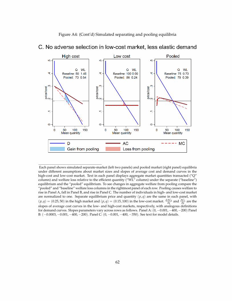
Figure A4: (Cont’d) Simulated separating and pooling equilibria


dqand AC1

dqare the


62

Table A1: Welfare changes by markup

Additional high cost market markup (%)

0 5 10 25 50 100

Low

cost

market

marku

p(%

)

0

0.17�0.110.10

65.52%

5

0.19 0.19 0.19 0.19 0.19 0.20�0.19 �0.19 �0.19 �0.20 �0.22 �0.250.10 0.10 0.10 0.10 0.10 0.09

51.94% 51.40% 50.87% 49.27% 47.95% 44.09%

10

0.21 0.21 0.21 0.21 0.22 0.23�0.26 �0.27 �0.27 �0.29 �0.33 �0.400.10 0.10 0.10 0.10 0.09 0.08

42.35% 41.47% 41.77% 39.16% 37.19% 31.24%

25

0.27 0.27 0.27 0.28 0.30 0.32�0.48 �0.49 �0.51 �0.57 �0.66 �0.860.10 0.10 0.09 0.09 0.08 0.05

26.58% 26.05% 24.66% 22.28% 18.25% 11.01%

50

0.37 0.38 0.38 0.40 0.43 0.49�0.84 �0.88 �0.92 �1.04 �1.25 �1.680.09 0.09 0.08 0.07 0.04 �0.01

15.01% 14.52% 13.43% 10.28% 6.02% �0.72%

100

0.57 0.59 0.60 0.64 0.71 0.85�1.56 �1.65 �1.74 �2.00 �2.46 �3.380.08 0.07 0.06 0.03 �0.02 �0.12

7.23% 6.46% 5.33% 2.49% �1.59% �7.79%

200

0.98 1.01 1.03 1.13 1.28 1.61�3.00 �3.20 �3.39 �3.97 �4.94 �6.880.06 0.04 0.02 �0.04 �0.15 �0.35

2.81% 1.85% 0.71% �1.81% �5.57% �11.18%

This table describes changes in changes in welfare loss before and following deletion.Cells are additional markups (columns, in percent terms) relative to a given markuprate in the low cost market (rows). Within each cell, rows are level changes in wel-fare loss in the low cost, high cost, mean change in welfare loss across both markets,and percent change in welfare loss relative to baseline loss the pooled market followingdeletion.

63

Table A2: Difference-in-difference predictions using long run default measures

Positive exposure Negative exposure

PredictedDefault

AverageCost

NewBorrowing

PredictedDefault

AverageCost

NewBorrowing

Jun. 2010 0.01 0.00 �7.09⇤ 0.03 0.03 �5.68+(0.02) (0.02) (3.05) (0.05) (0.05) (3.23)

Dec. 2010 0.01 0.01 �2.11 0.02 0.01 0.30(0.02) (0.02) (3.52) (0.05) (0.05) (3.25)

Jun. 2011 0.00 0.00 0.00 0.00 0.00 0.00(0.00) (0.00) (0.00) (0.00) (0.00) (0.00)

Dec. 2011 0.25⇤⇤⇤ 0.12⇤⇤⇤ �13.28⇤⇤ �0.30⇤⇤⇤ 0.04 17.98⇤⇤⇤(0.02) (0.02) (4.21) (0.04) (0.04) (3.47)

Elasticity 0.48 �0.24 �0.12 �0.36Dep. Var. Base Period Mean 0.08 0.08 214.70 0.14 0.14 165.09N Clusters 307 307 307 299 299 300N Obs. 2,929,133 4,961,674 13,163,613 1,486,567 2,519,339 8,117,207N Individuals 1,844,615 2,394,399 4,373,700 1,104,246 1,571,258 3,422,263N Exposed Individuals 452,132 765,941 1,967,865 79,572 134,306 589,628

Significance: + 0.10 * 0.05 ** 0.01 *** 0.001. Difference and difference estimates fromequation 1. Table is identical to Table 4 but uses a one-year ahead measure of default tocompute predicted default rates. See section 3 for details. The first two columns reportthe difference-in-difference estimated effect of deletion on outcome variables listed incolumn headers, while the third and fourth estimate the dif-in-dif effect on the differentexposure-defined markets. We take the log of ‘Predicted default’ for estimation butreport the base period mean in levels. ‘Elasticity’ is borrowing effect scaled by baseperiod outcome mean and predicted default effect. ‘N exposed individuals’ reports thenumber of individuals not in the zero group included in the regression sample in thetreatment period. Since some individuals appear in multiple snapshots we report bothindividuals and observations. Standard errors clustered at market level.

64

Table A3: Distribution of deletion effects using long run default measures

Separate Pooled DifferencePositive exposure

Predicted cost 0.065 0.081 0.016Average cost 0.065 0.073 0.008New borrowing (1000s CLP) 234.779 222.246 �12.533Welfare loss (1000s CLP) 1.711 2.138 0.427Aggregate new borrowing (Bns CLP) 447 424 �24Aggregate welfare loss (1000s CLP) 3, 261, 672 4, 075, 579 813, 908

24.95%N individuals 1, 905, 946 1, 905, 946 1, 905, 946Negative exposure

Predicted cost 0.120 0.081 �0.039Average cost 0.120 0.125 0.005New borrowing (1000s CLP) 112.490 132.079 19.589Welfare loss (1000s CLP) 0.140 1.128 0.988Aggregate new borrowing (Bns CLP) 67 78 12Aggregate welfare loss (1000s CLP) 83, 086 668, 656 585, 570

704.77%N individuals 592, 732 592, 732 592, 732Combined

Average cost 0.072 0.081 0.008New borrowing (1000s CLP) 205.770 200.857 �4.913Welfare loss (1000s CLP) 1.339 1.899 0.560

41.84%Aggregate new borrowing (Bns CLP) 514 502 �12Aggregate welfare loss (1000s CLP) 3, 344, 758 4, 744, 236 1, 399, 478

41.84%N individuals 2, 498, 678 2, 498, 678 2, 498, 678

This table describes changes in key welfare metrics before and following deletion, with inputs to thetheoretical framework using the long-run cost measure, assuming a 0% markup.

65

B Detail on the machine learning procedure

We generate cost predictions by regressing an indicator for new default against a largeselection of features using a random forest algorithm. We create four sets of predictionstrained on 10% of the data with new borrowing within each snapshot – approximately8% of the overall data. Predictions are trained and predicted either contemporane-ously, within each 6-month post-December snapshot (PD

post), or only in the Decem-ber 2009 snapshot (PD

pre). The random forests for each type are constructed with orwithout registry information. We use python’s sklearn package to perform our ma-chine learning tasks (Pedregosa, Varoquaux, Gramfort, Michel, Thirion, Grisel, Blon-del, Prettenhofer, Weiss, Dubourg, Vanderplas, Passos, Cournapeau, Brucher, Perrotand Duchesnay 2011).

Our random forest regression design constructs regression trees using a feature vec-tor of the following observable characteristics of each observation: a gender indicator,and one and two period lags of innovations in borrowing, innovations in total debt,total borrowing, total debt, average costs, and credit line information. We additionallyinclude the default history deleted from the credit registry in some of the trees. In total,these trees have either thirteen or fourteen predictor variables.

We scale our features by binning their nonzero values into quartiles. This reducesnoise in the feature vector and creates parsimonious regression trees. In our dataset, wefind that this additionally decreases the time necessary to construct a random forest.Finally, we subset over only new borrowers in each period so that our cost estimatesreflect costs conditional on borrowing.

To generate our PDpre predictions, we train a model only using observations in the

December 2009 snapshot. PDpost predictions are generated using a training sample

from each snapshot; these predictions are actually generated using a suite of modelseach tied to a particular snapshot.

We use three-fold cross validation combined with a grid search to pick parametersfor each model. The parameters over which we search are the minimum number ofobservations in a terminal node (minleaf ) and the number of features over which eachtree can sample. We set the number of trees in a forest to 150. Predictive power isnot sensitive to choices in this range. See figures B1 and B2 to see outcomes from thisprocedure.

Constructing random forests is (generally) a supervised learning task. Breiman(2001) defines a random forest as a set of regression trees, hk = h(x, Qk) where h isa tree and Qk is a random selection of observations and features from the training data,

66

where each tree “votes” on the output given an observation. We pick splits in the data toreduce mean-squared error, as is common with regression tasks. We use this loss func-tion and a regression task, despite our target variable existing only in {0, 1}, to ensurethat our outputs are continuous on [0, 1] and reflect probabilities. Our predictions arebest thought of as a weighted average of default rate in pools of observations clusteredtogether by similarity along a set of their covariates.

We additionally estimate a regression tree17 to bin borrowers into smaller markets.We define a market as a set of observations M such that h(xi, Q) returns a predictionstemming from the same terminal node for all i 2 M. We use this method to clusterborrowers into borrowers with similar features and default rates. These clusters there-fore represent infered groups in the data at the level which we believe the treatment isapplied and are analagous to the clusters defined in each tree in the forest.

Finally, we recreate the analysis above, exchanging the random forest algorithm fortwo other machine learning procedures that return classification probabilities. Theseare a naive Bayes classifier and a logistic LASSO. Our naive Bayes classifier first binsnonzero values along the feature vector into quartiles. Under the naive assumptionof independence of features in the feature vector, the classifier constructs P(default|X)

using Bayes’ formula under the assumption that P(X|default) is Gaussian, though thisis functionally irrelevant due to binning.

For the logistic LASSO, we take the log of nonzero values of continuous features,dummying out zero values using indicator variables. We perform a logistic regressionwith a l penalty term of the sum absolute value of the coefficients and use three-foldcross validation to pick l for each model.

Finally, we classify observations’ socioeconomic status by training a random for-est classifier on observations for whom the bank defined socioeconomic status group.Our three-fold cross validation procedure indicates that we are able to do this with ap-proximately 35% accuracy using a random forest composed of 100 trees and built on afeature vector consisting of continuous measures of consumer debt, mortgage amount,debt balance, credit line, bank default, average cose, age, total default amount, and in-dicators for gender, new borrowing, and having positive borrowing cap. See figure B3for cross-validation output.

17We estimate CART-style regression trees that split using variance reduction (Breiman, Friedman, Stoneand Olshen 1984).

67

Figure B1: Cross-validation output forPDpre random forest predictions

.18

.2.2

2.2

4.2

6.2

8A

ccur

acy

(R2 )

4 6 8 10 12Number of Trees

With Registry Info

.18

.2.2

2.2

4.2

6.2

8A

ccur

acy

(R2 )


Without Registry Info

Cross-validation (Pre-Period)

Minleaf = 1 Minleaf = 50 Minleaf = 100

68

Figure B2: Cross-validation output for PDpost random forest predictions

.19

.2.2

1.2

2.2

3.2

4A

ccur

acy

(R2 )


With Registry Info

.19

.2.2

1.2

2.2

3.2

4A

ccur

acy

(R2 )


Without Registry Info

Cross-validation (Pre-Period)


Figure B3: Cross-validation output for PDpost logistic LASSO predictions

.342

.344

.346

.348

Acc

urac

y (R

2 )



SES Class Predictions

69

internet appendix - pages.stern.nyu.edupages.stern.nyu.edu/~aliberma/lnoz_online_appendix.pdf ·...

Documents