International Journal of Heat and Mass Transfer 102 (2016) 959–970

Contents lists available at ScienceDirect

International Journal of Heat and Mass Transfer

journal homepage: www.elsevier .com/locate / i jhmt

Quality and reliability of LES of convective scalar transfer at highReynolds numbers

http://dx.doi.org/10.1016/j.ijheatmasstransfer.2016.06.0930017-9310/� 2016 Elsevier Ltd. All rights reserved.

⇑ Corresponding author at: CEE-EQuad-E414, Princeton University, Princeton, NJ08544, USA.

E-mail address: ebouzeid@princeton.edu (E. Bou-Zeid).

Qi Li a, Elie Bou-Zeid a,⇑, William Anderson b, Sue Grimmond c, Marcus Hultmark d

aDepartment of Civil and Environmental Engineering, Princeton University, USAbDepartment of Mechanical Engineering, University of Texas at Dallas, USAcDepartment of Meteorology, University of Reading, UKdDepartment of Mechanical and Aerospace Engineering, Princeton University, USA

a r t i c l e i n f o a b s t r a c t

Article history:Received 9 March 2016Received in revised form 26 June 2016Accepted 27 June 2016Available online 14 July 2016

Keywords:Forced convective heat transferLarge-eddy simulationRough wallsUrban heat exchange

Numerical studies were performed to assess the quality and reliability of wall-modeled large eddy sim-ulation (LES) for studying convective heat and mass transfer over bluff bodies at high Reynolds numbers(Re), with a focus on built structures in the atmospheric boundary layer. Detailed comparisons were madewith both wind-tunnel experiments and field observations. The LES was shown to correctly capture thespatial patterns of the transfer coefficients around two-dimensional roughness ribs (with a discrepancy ofabout 20%) and the average Nusselt number (Nu) over a single wall mounted cube (with a discrepancy ofabout 25%) relative to wind tunnel measurements. However, the discrepancy in Re between the windtunnel measurements and the real-world applications that the code aims to address influence the com-parisons since Nu is a function of Re. Evaluations against field observations are therefore done to over-come this challenge; they reveal that, for applications in urban areas, the wind-tunnel studies result ina much lower range for the exponent m in the classic Nu � Rem relations, compared to field measure-ments and LES (0.52–0.74 versus � 0.9). The results underline the importance of conducting experimentalor numerical studies for convective scalar transfer problems at a Re commensurate with the flow of inter-est, and support the use of wall-modeled LES as a technique for this problem that can already captureimportant aspects of the physics, although further development and testing are needed.

� 2016 Elsevier Ltd. All rights reserved.

1. Introduction

Convective heat and mass transfer at high Reynolds numbers(Re � 106–108) over complex surfaces is of interest for many engi-neering and environmental applications, such as heat exchangerdesign, agricultural and urban meteorology, and building energystudies. The latter applications are of growing significance due torapidly expanding urbanization interacting with global climatechange to alter the urban environment and the resource intensityof cities in complex ways. The convective heat transfer coefficientover the exterior surfaces of buildings is a key parameter for mod-eling the exchange of energy between buildings and their environ-ment. This exchange needs to be quantified to calculate accurateheating and cooling loads [1,2], to assess the energy performance

of the building envelope [3], and to better simulate the urban envi-ronment under a changing climate [4].

In addition, with the heat-mass transfer analogy [5], knowledgeon the turbulent transfer of temperature (under conditions whereit can be considered as a passive scalar) is transferable to studieson the exchange of other scalars, especially carbon dioxide andmoisture [6], which are important for example for assessing theperformance of green roofs [7,8]. For urban climatological andmeteorological studies, it is crucial to simultaneously capture theturbulent heat and water vapor surface fluxes, which are typicallyparameterized through an urban canopy model (UCM) [9–12] incoarse geophysical simulations. The transfer coefficients for heatand water vapor are important parameters in these UCMs [13],but their current parameterizations are partially based on experi-mental results that are over 90 years old [14]. Improved parame-terizations would involve environmental turbulent boundarylayer flows over large roughness elements the height of whichcan be a significant fraction of the total boundary layer depth. Suchsurfaces are termed very rough in Castro et al. [15] and theresulting flow differs from the classic rough-wall boundary layers

Nomenclature

cp specific heat at constant pressurehc heat/mass transfer coefficient qs/(s0 � sref)H height of the obstacle (rib or cube)Li LES domain size in direction im power exponent in Nu–Re relationRe Reynolds number = uH/ms scalar concentrationu characteristic velocity scaleu⁄ friction velocity = (�sw)1/2, where sw is the total kine-

matic wall shear stressz0m momentum roughness length

z0s scalar roughness lengthx, y, z streamwise, cross-stream and vertical coordinatek heat conductivity of solid surface

Subscriptsx, y, z streamwise, cross-stream and vertical directionsLES quantities from LESExp quantities from experiments0 quantity at surfaceref quantity at reference height

960 Q. Li et al. / International Journal of Heat and Mass Transfer 102 (2016) 959–970

discussed for example in Jiménez [16] where the height to bound-ary layer depth ratio is limited to be below 0.025. Advancing ourunderstanding of the fundamental transport processes of heatand moisture over such complex surfaces, and how to model themvia transfer coefficients beyond the current state of the science, ishence urgently required in view of the wide range and importanceof the related applications.

Three different approaches have been traditionally taken to gaina better understanding of the convective transfer coefficients. Thefirst approach is placing scale models in wind tunnels and measur-ing the convective transfer of either some substance or tempera-ture, while minimizing the effect of buoyancy (which couldnonetheless be quite important in real urban terrain). These stud-ies [17–24] often considered cases at lower Reynolds numbers(103–104) (due to length scale limitations), with a developing tur-bulent boundary layer in a parallel channel flow. Mass transferexperiments, usually with Naphthalene sublimation techniques[18,25] or water evaporation [23], were performed to study themass transfer from surface-mounted cubes in a wind tunnel. Theseare only some examples of wind tunnel studies from the extensiveliterature, which was summarized in relatively recent reviews[2,3]. One advantage of wind tunnel studies is that the spatial vari-ation of heat/mass transfer coefficients along the surfaces of thebluff elements can be accurately measured. The setup of the exper-iments can also be varied to investigate the effects of differentangles of attack [19] and geometric configuration of the roughnesselements [17,23], among other topographically complexities. How-ever, a simple extension of these studies to the environment has tobe handled with caution. The Reynolds number of the typicalatmospheric boundary layer (ABL) is 3–4 orders of magnitudehigher than that of common wind tunnels. Unlike momentumexchange, which is fully dominated by form/pressure drag overcomplex topographies at high Re, heat and mass exchanges arealways performed by molecular conduction or diffusion in thevicinity of the complex interface and do not lose their dependenceon the molecular heat and mass diffusivities at high Re. Neither theconvective to conductive/diffusive scaling represented by the Nus-selt number for heat (Nu) or Sherwood number for mass (Sh), northe inertial scaling given by the Stanton number (St � Nu/Re),become independent of Re in general (See Lienhard and Lienhard[26]). Re-independence for St might be approached or expectedonly if the flow over each facet is itself also fully rough [27], whichis not always the case over urban terrain since the surfaces ofbuilding facets might be smooth or transitional. The empirical cor-relations of Nu, Sh, or St with Re obtained from these scale modelexperiments are thus not directly applicable to heat or mass trans-fer from buildings [23]. In addition, the usually thin inflow turbu-lent boundary layers [2] and the low turbulent intensity levels arefurther reasons why wind tunnel studies of heat and mass transfer,

although providing very valuable insight, have limitations that pre-clude the direct application of their findings to large scale flows athigh Re, such as flows in the real natural environment [28].

Another approach that overcomes the problem of low Re inwind tunnel studies is full-scale experiments conducted outdoorson buildings or structures [29–33]. These field experiments givevery valuable information especially on the correlation betweenthe heat transfer coefficient and wind speed, which can be gener-alized to a power-law relation between Nu and Re. One manifesta-tion of the continued dependence of heat and mass exchange on Reis that the exponents in such power laws are themselves Re depen-dent, and thus these empirical relations apply only in the range ofRe in which they were developed. From the perspective of model-ing, such full-scale field-derived empirical relations are thereforeuseful for both building energy simulations and urban climatestudies [1,13]. However, generalization of the findings can alsobe challenging due to the influence of the exact shapes of the build-ing facets, the texture/roughness of the building surface materials,and the surrounding structures in the outdoor environment. Inaddition, the positions at which the temperature and wind velocityare measured vary across different field studies, further complicat-ing inter-comparisons between them to extract more universalempirical relations.

Numerical simulations are another useful methodology to studythis problem. Reynolds averaged Navier–Stokes (RANS), large-eddysimulations (LES) or direct numerical simulations (DNS) have beencarried out in the recent years to study the turbulent transfer ofmomentum and scalars over rough surfaces with roughness ele-ments that mimic buildings or urban canyons [34–37]. Since thecomputational cost of resolving the viscous layer (i.e. DNS [38–41] or wall-resolved LES [42]) is too high for applications at Recommensurate with the real-world (limiting these techniques tolow Re where the same challenges discussed above for wind tun-nels reemerge), wall modeling is often adopted for RANS or wall-modeled LES studies. The ‘law of the wall’ or related equilibriumapproaches, which are based on the concept of universal behaviorof momentum and scalars in the inertial (logarithmic) layer, areoften adopted [34,35,43–45]. These types of wall models havesome known caveats in complex flow regions [46]; however, goodagreement of models using such equilibrium laws with experi-ments have been found by both Park et al. [34] and Liu et al. [44]in their studies of transfer of scalars over geometrically complexsurfaces. The application of such equilibrium wall-models in LESpose additional challenges (compared to RANS) that were verycomprehensively assessed by Wyngaard et al. [47]. Various othermore sophisticated wall-models that should in principle offer bet-ter performance have been proposed such as models that solve theboundary layer equations numerically [48] or analytically [49,50],or models that use a ‘‘customized temperature wall function”

Q. Li et al. / International Journal of Heat and Mass Transfer 102 (2016) 959–970 961

(CWF) (though based on low Reynolds number results) [51]. Nev-ertheless, the challenge of wall-modeling in LES remains open[52,53], even when the very important influence of buoyancy andhow to represent it correctly in wall models (particularly for verti-cal walls) is ignored. This challenge frames the scope and goals ofthis paper.

Given that for studies of turbulent flow and transport overurban-like rough surfaces at high Re wall-modeled LES is a feasibleand very appealing tool, there is a growing urgent need to assess itsskill in capturing turbulent scalar transport. The near-surface per-formance is more critical for scalars than for momentum (againdue to the dominance of form drag, which is partially resolved inLES, for momentum), and as such the role of the wall-model ismore prominent. But if the shortcomings of current wall modelscan be investigated, quantified, and potentially overcome, theimpact on future studies that focus on scalar transport under highRe scenarios can be substantial. It is worthwhile to stress again theimportance of studying the heat/mass transfer problem at a Rey-nolds number that is representative of the real problem of interest(which is possible with wall-modeled LES), given that the scalartransfer is inherently Re-dependent.

Therefore, the objective of this study is to provide a thoroughassessment of wall-modeled LES by detailed comparisons to bothscale-model and full-scale studies. Knowing the capabilities andlimitations of this numerical approach will help to draw more sen-sible conclusions for future applications in building energy andurban climatology studies. A practical question we seek to answeris: are the errors resulting from the parameterization of unresolvedscales (wall and subgrid scale models) in LES larger or smaller thanthe errors involved in extrapolating from low-Re approaches (DNSor wind tunnels) to high-Re real world flows, for scalar transferproblems?

This paper is organized as follows: section two describes thenumerical details of the large eddy simulation; section three dis-cusses the comparison of the local scalar transfer coefficient withwind-tunnel studies of two-dimensional roughness; section fourconsiders both the local and average transfer coefficients by com-paring to wind-tunnel studies of a single cube; section five focuseson the comparison with full-scale field measurement, section sixprovides a summary and conclusions.

2. Wall-modeled LES and dynamic roughness wall model

The LES code uses the immersed boundary method (IBM) toaccount for presence of the roughness elements, in which a dis-crete time momentum forcing is used to simulate the immersedboundary force [54,55]. The filtered incompressible continuity,Navier–Stokes and scalar conservation equations (Eqs. (1)–(3),respectively) are solved assuming hydrostatic equilibrium (we willomit the usual tilde above the variables that denotes filtering forsimplicity, but all the variables we will discuss are the filtered/resolved components solved for in LES unless otherwise noted)

@ui

@xi¼ 0; ð1Þ

@ui

@tþ uj

@ui

@xj� @uj

@xi

� �¼ � @p

@xi� @sij

@xjþ Fi þ Bi; ð2Þ

@s@t

þ ui@s@xi

¼ � @qsi

@xi; ð3Þ

where t denotes time; ui is the resolved velocity vector; p is themodified pressure; sij is the deviatoric part of the subgrid stress ten-sor; Fi is the body force driving the flow (here simply a homoge-neous steady horizontal pressure gradient along the x direction);

and Bi is the immersed boundary force representing the action ofthe obstacles (buildings) on the fluid. The density is assumed equalto 1 (all the equations are normalized so the numerical value of thedensity is irrelevant). In Eq. (3), s denotes a passive scalar quantityand qs

i is the ith component of the subgrid scale scalar flux.Although the code can simulate active scalars (see [56,57]), theexperimental data we identified for code evaluation were underconditions where buoyancy played an insignificant role.

The code uses a pseudo-spectral method for computing the hor-izontal spatial derivatives on a uniform staggered Cartesian grid.To overcome the Gibbs phenomenon that emerges from the com-bined application of the IBM method with spectral derivatives, asmoothing approach we developed and detailed in Li et al. [58] isadopted. Vertical spatial derivatives are obtained from second-order centered finite difference. Second order Adams–Bashforthtime integration is used. The subgrid scale (SGS) stress tensor ismodeled using the Lagrangian scale-dependent dynamicSmagorinsky model [59], while the SGS scalar flux model usesthe dynamically computed SGS viscosity with a constant SGSPrandtl number (PrSGS) of 0.4 (this is unrelated to the molecularPr [60]).

In this study, we adopt a new approach for dynamically evalu-ating the momentum and scalar roughness lengths in the expres-sion of the log-law wall model. The general log-law wall modelfor momentum and scalars is given by:

uu�

¼ 1j

logzz0m

� �; ð4Þ

s0 � ss�

¼ 1j

logzz0s

� �; ð5Þ

where u is the local wall-parallel velocity near the wall; s0 is thescalar concentration or temperature at the surface; u⁄ is the frictionvelocity calculated as the square root of the kinematic wall shearstress sw; s⁄ is the mass flux concentration or heat flux temperature(defined as the kinematic surface flux divided by u⁄); z is distanceaway from the wall in the wall-normal direction; j = 0.4 is thevon Kármán constant; and z0m and z0s are the roughness lengthsfor momentum and scalars, respectively. These roughness lengthsare often chosen according to the roughness types of the surfacesfor hydrodynamically rough walls. However, building facets areoften hydrodynamically smooth, including the experiments wecompare to. Therefore, instead of adopting a fixed roughness, wedynamically model the roughness lengths for momentum and sca-lars as a function of the viscous length scale m/u⁄. In fact, it has beenshown by Kader and Yaglom [61] that similar reasoning to the onethat yielded the Prandtl–Nikuradse momentum skin friction law forsmooth pipe and channel flow can be applied to scalar transfer in aturbulent flow to obtain heat or mass transfer laws for a smoothwall, with some unknown quantities that can be determined fromexperiments. Eq. (4) can be rewritten following the Prandtl–Niku-radse skin friction law as

uu�

� �¼ A log

zm=u�

� �þ B; ð6Þ

which can be further rearranged into

u� ¼ u

A log z eB=Am=u�

� � ¼ u

A log zz0m

� � ; ð7Þ

where A and B are determined from experiments and z0m is given by

z0m ¼ mu�

e�B=A: ð8Þ

The same dimensional analysis can then be similarly developedfor scalars:

962 Q. Li et al. / International Journal of Heat and Mass Transfer 102 (2016) 959–970

s0 � s ðzÞ ¼ s�w ðu� z=m; m=vÞ; ð9Þ

where v is the mass or thermal diffusivity, and w is a dimensionalanalysis function to be determined empirically (with the aid ofprofile-matching as for velocity). Eq. (9) is a general one for turbu-lent mass or heat transfer in wall-bounded flows. For air, Pr = 0.7and s� ¼ qs=ðqcpu�Þ, where qs is the dynamic heat flux at the walland cp the heat capacity of the air. The experiments to determinethe form of Eq. (9), as detailed in Kader and Yaglom [61], then yieldthe log-law for scalar:

s0 � s ðzÞs�

¼ a logz

m=u�

� �þ b : ð10Þ

For air, a and b can be found from experiments for heat transferwith weak buoyancy. If s represents air temperature, then the heatflux at the wall is given by

qs

qcp¼ u�s� ¼ u�

ðs0 � sðzÞÞa log z eb=a

m=u�

� � ¼ u�ðs0 � sðzÞÞa log z

z0s

; ð11Þ

where z0s for the scalar can be written as:

z0s ¼ mu�

e�b=a: ð12Þ

The roughness length expressions in Eqs. (8) and (12) should beuniversal for smooth walls, and thus we can adopt the constantsdetermined by Kader and Yaglom from experiments for fully tur-bulent flows [61,62] (Table 1 in Kader and Yaglom [61]; A can beviewed as the inverse of the von Kármán number, but only theratios B/A and b/a influence the results and here we select the sameratio of 3.9/1.8 for both momentum and scalars, which effectivelyyield

z0m ¼ z0s ¼ m8:73u�

’ m9u�

: ð13Þ

This result applies for molecular Prandtl of Schmidt numbers�1, which is a reasonable approximation for all the tests we con-duct in this study. These length scales depend on u⁄ which variesin space and time over complex geometries. We thus use an expli-cit approach where u⁄ form the previous time step is used in Eq.(13) to determine z0m at every wall location, and then the updatedz0m is used to compute u⁄ from Eq. (7). This dynamic equilibriumwall-model controls the fluxes at the solid–fluid interface, andtherefore is important to determine if the LES is able to capturethe physics of the flow and reproduce experimental observations.It is important to note here that this model, by construction sinceit assumes smooth facets, yields a Stanton number that is Redependent. On the other hand, if the facets were assumed fullyrough with constant z0m and z0s, the heat transfer regime wouldbecome Re independent. We assume the presence of a logarithmicform at the first grid point away from the wall of the solid, which iscommonly done in direct forcing immersed boundary method asadopted here.

Table 1The absolute percentage deviation (%), |(hLES – hExp)/hExp| � 100, of the averagedtransfer coefficient over each facet and all facets combined.

Leeward Street Windward Roof Average

W/H = 1/2 18.2 15.5 20.3 42.3 25.5W/H = 1 11.1 12.0 30.2 35.5 22.5W/H = 2 20.2 22.5 17.4 27.8 22.0

3. Spatial variation of the transfer coefficient compared to awind tunnel study

3.1. Experimental setup of mass transfer over two-dimensional ribs

The dimensional (e.g. in W K�1 m–2) local heat or mass transfercoefficient is defined as

hc ¼ qs

s0 � sref; ð14Þ

where sref is some reference scalar quantity in the fluid. The distri-butions of the local heat and mass transfer coefficients obtainedfrom detailed scale-model measurements have large spatial varia-tions over the surface of roughness elements due to the highly com-plex flow patterns involving separations and reattachments in theflow. It is therefore desirable to assess the capability of the wall-modeled LES in predicting these spatial patterns of local heat andmass transfer coefficients.

Nevertheless, one here again faces the challenge that the mag-nitudes of hc in scaled-model experiments at lower Re and LES atlarger Re are not directly comparable due to the dependence ofhc on Re. However, since the momentum dynamics are less sensi-tive to Re, the spatial flow patterns should match as long as thescaled-model Re exceeds �105, and therefore the resulting spatialvariation patterns of hc should be comparable. Therefore, to over-come the magnitude discrepancy and still compare the spatial vari-abilities, the heat or mass transfer coefficients from different scale-model experiments and numerical simulations are usually normal-ized for appropriate comparison [13].

The measurement of mass transfer coefficient from a wind-tunnel study on evaporation of water from two-dimensionalroughness (ribs) by Narita [23] is used here as a benchmark caseto assess the LES. The roughness elements, made of acrylic resinof 1 mm thickness, were covered with wetted filter paper. A finethermistor sensor was inserted just below the paper surface tomonitor the surface temperature. The evaporating surface isassumed to be at saturation. A weighing method was used toobtain the evaporation rate and thus the mass transfer coefficientcan be estimated by knowing the ambient water vapor concentra-tion. Measurements were conducted at a low relative humidity tokeep the experimental error of the transfer coefficient to within 4%.

Note that the sharp edges of these 2D ribs fix the separationpoints to the downstream top corners of each rib, and thusstrengthen the insensitivity of the flow patterns to Re and improvethe flow simulation results [63].

3.2. Numerical model of mass transfer

We considered configurations with three different separationdistances between the two-dimensional ribs. Fig. 1 is a side viewof the basic configuration. The rib height H is represented with16 grid points. We use a horizontally periodic boundary conditionfor momentum and mass (thus we are simulating infinite repeti-tions of the patterns shown in Fig. 1). The longer section behindthe ribs is used to ensure that the inflow velocity at the first ribis free of the wake influence from the fifth element. It also mimicsthe test section surface upstream of the ribs in the open circuitwind tunnel [23]. The experimental Reynolds number is 16,000,where velocity is fixed at 4m/s at the top of the boundary layerand length scale is the rib height. The experiment did not preciselycontrol the humidity in the incoming air in the wind tunnel.Instead, during each run where the evaporation rate was mea-sured, the evaporation rate from a flat plate placed in the freestream was simultaneously recorded for normalizing the measure-ments. Therefore, we could not replicate the exact details of the

W/H = 0.5

W/H = 1

W/H = 2

W

H

Nx = 256

Nx =288

W

H

H

W

Nx =320

zy

x

1 2 3 4 5

roofleeward windward

street

Fig. 1. Side view of the geometric configuration of the numerical simulations. The cases ofW/H = 0.5, 1 and 2 are shown in the figure from top to bottom. Inflow is from left toright. Nx is the number of grid points in x-direction. Nz = 80 total vertical grid points for all three cases.

Q. Li et al. / International Journal of Heat and Mass Transfer 102 (2016) 959–970 963

mass inflow, but again these only affect the magnitude and not thespatial patterns of the transfer coefficient that we seek to investi-gate here.

The top boundary condition in the simulation is slip-free formomentum and zero-flux for the scalar (same top BC for all simu-lations in this paper). The dimensions of the wind tunnel are 0.9 min height and 1.8 m in width. The height of the wind tunnel is 15times the height of the rib H = 0.06 m We have conducted prelim-inary tests by varying the domain height from 3 times to 10 timesH (results not shown here) to test the sensitivity to the domainheight. We found that results with domains exceeding 5H in heightconverge, and therefore we adopt 5H as our domain height in allsimulations in this section. The boundary condition on the surfacesof the ribs for water vapor is assumed to be at a constant concen-tration, which is justified by the saturated state of the wetted sur-

Fig. 2. Mean (time- and y-averaged) contour plots of s/s0 and streamlines. The wind is frodimensional ribs. Color scale for the normalized scalar concentration is the same for allreader is referred to the web version of this article.)

faces. All cases were run for about 20 eddy turn over times (Lz/u⁄)and averaged in the y-direction, to reach statistical convergence,which was further confirmed by ensuring that the velocity profilesreach a steady state, i.e. they become invariable if the averagingtime is further increased.

Fig. 2(a)–(c) shows the pseudocolor plots of the scalar concen-tration normalized by the surface scalar concentration, togetherwith the streamlines. The central vortices in the W/H = 0.5 and 1cases are characteristic of the ‘skimming flow’ regime and explainthe high concentrations of scalar in the space between the ribs(‘‘the street canyon”), whereas the slightly asymmetric flow fieldin case W/H = 2 is evidence of more complex flow interactions inthe ‘wake interference regime’ [64,65] that allows more exchangebetween the canyon and the air aloft. The flow patterns are consis-tent with the regime expected for this geometry. In addition to the

m left to right. The white spaces represent the transect areas occupied by the solid 2-three cases. (For interpretation of the references to colour in this figure legend, the

Fig. 3. Snapshots of instantaneous s/s0 and streamlines. The wind is from left to right. The white spaces represent the transect areas occupied by the solid 2-dimensional ribs.Color scale for the normalized scalar concentration is the same for all three cases. (For interpretation of the references to colour in this figure legend, the reader is referred tothe web version of this article.)

964 Q. Li et al. / International Journal of Heat and Mass Transfer 102 (2016) 959–970

more intensive exchanges for the widest canyon, the reduced‘‘emitting surface” to ‘‘canyon volume” ratio, (W + 2H)/(HW) = H+ 2/W, when W increases and H is maintained constant, furtherexplains the reduced concentrations in the canyon.

Fig. 3(a)–(c) shows instantaneous contour of the scalar concen-tration normalized by the surface scalar concentration, togetherwith the streamlines along one xz-slice at a fixed y. The instanta-neous structures in the scalar concentration field, as well as thestreamlines, are generally distinct from their averaged counter-parts shown in Fig. 2, particularly for the W/H = 2 case. Thedepicted turbulent structures are important for the verticalexchange; for example, one can observe the strong ejection fromthe last canyon in Fig. 3(c) for the W/H = 2 case. This is consistent

0 0.5 1 1.5 2 2.5 3 3.5L/H

0

2

4

6

hc/h

0

(a) W/H = 0.5

Narita(2007)LES

0 0.5 1 1.5 2 2.5 3 3.5 4L/H

0

1

2

hc/h

0

(b) W/H = 1

0 0.5 1 1.5 2 2.5 3 3.5 4 4.5 5L/H

0

1

2

hc/h

0

(c) W/H = 2

Roof Leeward Street Windward

Fig. 4. The normalized mass transfer coefficient for different positions across thecanyon. L is the path length along the interface, and a unit L/H is the length of thedotted line indicated in Fig. 1 for case W/H = 2 as an example. The white space withno data for the cases in (a) and (b) does not reflect a data gap, but the fact that thestreet widths are shorter in these cases compared to the case in (c), which we adoptto fix the overall width of the figure.

with general observations for such kind of type-k roughness wherethe eddies of scale H are shed out of the cavity, resulting in themore complex flow interactions. The instantaneous vortices insidethe canyons for the two other cases, especially W/H = 1 in 3(b), aresomewhat more similar to their time and space averaged counter-parts in Fig. 2(b). This dominant mean circulation inside the can-yons for these cases might hinder ejections and sweeps near thetop of the canyons and reduce the instantaneous exchangebetween canyons and air above. While we show only one snapshothere; other snapshots we analyzed conveyed the sameinformation.

Fig. 4 shows the comparisons between the experimental andLES results for the three rib separations, while Table 1 lists theabsolute percentage deviation of the LES from the experiments.All quantities are normalized by the average mass transfer coeffi-cient on the floor in between two consecutive ribs. The experimen-tal data are averaged over multiple ribs starting where the transfercoefficient over subsequent ribs converge. To best mimic theexperimental data, we average the LES result using relevant quan-tities from the second to the fifth rib, where the transfer coeffi-cients become independent of location of the ribs. We testeddifferent averaging ranges and the impact on the results is minimalThe resulting general spatial trends for each case, as well as thechanges in transfer coefficient patterns as a result of the variationin the separation distance, are adequately captured by the LES.Despite the fact that the leeward transfer coefficient varies quiteconsiderably across different cases, its variation is captured well:for example, the peak for W/H = 1 was observed to occur at about0.4H from the bottom and this maximum is also clear in LES. Boththe experiment and the LES also show that the decrease along thatface at W/H = 0.5 is more pronounced than W/H = 2. The variationon the street face (floor between two ribs) is also reasonably cap-tured by the LES. The maximum of the transfer coefficient on thestreet occurs at about 0.5H in the experiments for cases W/H = 1and W/H = 2, which is also the location predicted by the LES. Thispeak matches the location of the highest wall-parallel velocity pro-duced by the recirculating flow in the canyon. Given the complex-ity of the wakes and recirculation inside the canyon, the matchingof the observed time-averaged transfer coefficients that are modu-

0 1 2 3

u/u

0.1

0.2

0.5

1.0

2.0

3.0

5.0

z/H

0 0.2 0.4

TI

0.1

0.2

0.5

1.0

2.0

3.0

5.0

z/H

LESNarita (2007)

Fig. 5. The comparison between the mean streamwise velocity and turbulentintensity TI at the inflow section between LES and experiment.

zy

Lz = 4H Nz = 120

Top of domain: impermeable & stress free

Q. Li et al. / International Journal of Heat and Mass Transfer 102 (2016) 959–970 965

lated by these flow patterns indicate that the wall-modeled LES iscapable of reproducing them, as well as the spatial distributions ofthe local mass transfer they generate inside the canyon.

Larger discrepancy between the observations and LES occursnear the top of the windward facet and on the roof, which can havetwo possible reasons. One potential reason for this larger discrep-ancy is the difference in the dominant drag mechanism: whilepressure drag dominates at the vertical wall, the viscous drag dom-inates over the roof [66]. Another reason is related to our inabilityto match the experimental inflow conditions in LES exactly, asshown in Fig. 5. The inflow vertical profiles of the normalized meanstreamwise velocity and turbulent intensity (TI) at the upstream oflocation x = 0 are shown in Fig. 5. The mean velocity in both LESand experiment is normalized by its value at z = H, while the TI iscomputed locally. The mass transfer from the roof surface andupper part of the front/windward wall are more dependent onthe inflow profile (mean velocity as well as turbulence intensity)than the bottom and the leeward faces. To test the sensitivity ofthe mass transfer for the different faces to inflow conditions,another test was conducted also assuming a fully periodic domainbut without the long extension. This implies an infinite array ofribs, and is further removed from the actual setup in the wind tun-nel. The results from this test (not shown here) indicate that whilethe absolute value of the error defined as |(hLES–hExp)/hExp|remained similar for the leeward and bottom faces, the errors onthe front and top faces were 3–5 times larger compared to the val-ues presented in Table 1, which correspond to the basic setup. Thisfurther confirms the importance of characterizing the inflow inexperiments accurately and reporting it in the associated paperto allow the data to be used for model validation, and supportsour explanation that the higher discrepancy in the upper part ofthe windward facet and on the roof are related to a mismatch inthe inflow.

Lx = 4H Nx = 120

Horizontally periodic

xInflow

Ly = 4H Ny = 120

H

Fig. 6. Schematic drawing of the setup of the numerical simulation. A heated cubeof size H is placed in the middle of the domain. The grid consists of 1203 nodes, andthe domain size is Lx = Ly = Lz = 4H.

4. Facet-averaged heat transfer from a cube compared to a windtunnel study

4.1. Experimental set-up of heat transfer from a single cube

The turbulent forced convective heat transfer over a wall-mounted cube at relatively low Reynolds number has been quiteextensively studied as discussed in the introduction. In particular,we will focus on the study by Nakamura et al. [22] since theirexperiment was conducted at a relatively high Re – from 4200 to

33,000 – despite the fact that is remains orders of magnitude lowerthan for real buildings. Furthermore, relations between Nu and Refor different faces of the cube were proposed in that study, andthey will be useful for our comparisons. In this experiment, a cop-per cube was heated by an embedded heater to maintain the sur-face temperature approximately constant (within ±0.5 �C). Thecube, with a dimension of 30 mm, was placed in a low-speed windtunnel of 4 m height, 3 m width, and 8 m length. A turbulentboundary layer is achieved by placing a horizontal circular cylinder500 mm upstream from the cube to act as a trip. The diameter ofthe circular cylinder is 10 mm and the boundary layer depth tocube height ratio varies from 1.5 to 1.83. A temperature differenceof approximately 10 �C is maintained between the surface of thecube and the air temperature. Re, defined based on the cube heightand the bulk velocity upstream of the cube, was varied to assesshow it is related to Nu.

4.2. Numerical model of heat transfer from a single cube

For all simulations in this section, a horizontally periodicdomain is used. Fig. 6 is the schematic drawing of the setup ofthe numerical simulation. 30 grid points are used along each sideof the cube. The domain height is 4H, where H is dimension ofthe cube. The upper boundary condition is impermeable with afree-slip for momentum and zero-gradient (no flux) for tempera-ture. Five different simulations were performed at different Rey-nolds number in our LES by varying the horizontal pressureforcing, which is equivalent to changing the bulk velocity in theinflow. The Reynolds number is defined as Re = UH/m, where U isthe free stream velocity in the wind tunnel. The LES velocity usedin Re is taken at the location (x, z) = (0, 1.5H), which provides a rea-sonable match to the experimental definition. Notice that in theLES setup the wall model defines an inner scale (since we are usinga smooth-wall roughness length parameterization that depends onm), and the nominal Re of the simulations can therefore be deter-mined; viscous stresses are neglected in the numerical integrationof the momentum and scalar equations.

For all simulated cases, a constant temperature wall boundarycondition is implemented in the wall model. All cases were simu-lated for a total of 100 eddy turnover times, defined as Lz/u⁄ (thiscorresponds to 400 eddy turnover times defined based on the cube

Table 2The coefficients and exponents in Eq. (15) as determined in Nakamura et al. [22].

a m

Front 0.71 0.52Side 0.12 0.70Rear 0.11 0.67Top 0.071 0.74Cube average 0.138 0.68

966 Q. Li et al. / International Journal of Heat and Mass Transfer 102 (2016) 959–970

scale). After a transient of 50 eddy turnovers, all time-averagedstatistics reported were computed using the last 50 eddy turnoverstimes.

Fig. 7(a) shows a vertical x–z transect along y = 2H (middle ofthe cube), where both the contour of temperature deviation fromthe inflow temperature, defined as (h – hi)/hi, and the velocitystreamlines are shown. Similarly, Fig. 7(b) is a horizontal transectat z = 0.015H (near the floor). The temperature deviation contoursdepict large spatial gradients around the cube. The separation nearz = H/2, and the reattachment zone near the lower corner of thefront face of the cube (Fig. 7(a)) compare well with experimentalvisualizations [22,67]. The separation zone and the two counter-rotating vortices shown in Fig. 7(b) near the rear face are also somewell-known features of flow around a single cube, as seen forexample in flow visualizations in Nakamura et al. [22] and Martin-uzzi and Tropea [67].

The Nu–Re relation obtained from experimental measurementsof Nakamura et al. [22] follow the classic power law

Nu ¼ aRem; ð15Þthe coefficients of which are given in Table 2. Due to the differencein Re, these experimental Nu–Re relations of Nakamura et al. areextrapolated to the Re of the LES for comparison. This ignores thewell-known dependence of m on Re, a caveat we will revisit inthe next section. However, this approach was necessary sincereducing our Re further to match the experiment would place ourfirst grid point in the viscous or buffer layers and preclude us fromtesting the wall-modeled LES configurations that we aim to use forfull-scale (real-world) applications.

Fig. 8(a) shows the comparisons between the relations pro-posed by Nakamura et al. [22], extrapolated to the LES Re, for theaveraged Nu on different facets and the LES results. Although theseexperimental relationships were found at Re orders of magnitudesmaller, the match between predicted values according to Eq.(15) and those obtained from LES is in fact reasonable. The frontand leeward faces show higher errors than the other faces, buterrors cancel out and cube-averaged fluxes match quite well. Thiscan be interpreted either as giving confidence in the performanceof LES, or alternatively in the applicability of extrapolations fromlow Re studies to the higher Re flows in the real-world. Fig. 8(b)shows that the ratio of deviation Rd defined as:

Rd ¼ NuLES=NuExp; ð16Þwhere the experimental results are the values predicted from Eq.(15) and Table 2, at different Re. Except for the front face which isexcluded from this comparison, exchanges from the other facesremain within 50% of the measurements. The most likely reason

Fig. 7. Mean flow field (streamlines) and contour plot of the temperature deviation fromfloor at z = 0.015H.

why the front face deviates the most from the experimental resultis that the experimental flow over that face could still be in a regimeof laminar or transitional flow. This is strongly suggested by thesmall experimental exponent, 0.52, which is considerably lowerthan that expected in turbulent flows, and rather very close to the0.5 limit expected for laminar flows [68]. In addition, the turbulentboundary layer depth in the experiment is 1.5d/H, which is differentthan the fully developed one in LES of 4d/H.

It is often of practical interest to use the cube-averaged or facet-averaged value of the heat transfer coefficient when consideringthe bulk heat exchange between a building envelope and the sur-rounding air, despite the high spatial variability. Fig. 9(a) shows thecontours of the heat transfer coefficient normalized by the cubeaverage. Only one side-face is shown because of symmetry. Largedeviations from the cube-averaged value occur on the edges asexpected. The spatial variation at the intersections between front,top and rear faces is the most prominent. Fig. 9(b) depicts the heattransfer coefficient normalized by the respective face-averagedvalues. Despite the large spatial variability at the intersectionsbetween difference faces, the cyan contour of value 1.1 indicatesthat the deviation over a large area of each face is only moderate.This implies that for practical applications, point-measured valuesin the center of a facet or numerically-determined face-averagedvalues give good estimates of the transfer over larger portions ofeach facet, despite some loss of information on the higher valuesnear the corners. However, cube-averaged values should not beapplied to individual facets. The contour plots in Fig. 9 also com-pare well qualitatively with results in the experiments of Naka-mura et al. [22].

The wall friction velocity u⁄ and temperature scale h⁄, whereh� ¼ q0=ðu�qcpÞ, are shown in Fig. 10(a) and (b) respectively. Thespatial variability patterns of u⁄ are strongly correlated with thoseof hc, indicating that the friction velocity has a strong impact onheat transfer as expected. The patterns of h⁄ on the other handare distinct, with strong heat exchange near the bottom of the allfaces due to the horseshoe vortex depicted in Fig. 7.

Separate sensitivity tests with varying domain heights of 1.7Hand 3Hwere also conducted and yielded markedly different results

hinflow along (a) a vertical x–z plane at y = 2H; and (b) a horizontal plane close to the

2 3 4 5 6Re 108

104

105

106

Nu

FrontTopRearSideAverage

104 105

Nu (Experiment)

104

105

Nu

(LE

S)

50%

25%

-25%

-50%

Fig. 8. (a) Nu–Re relation for different faces using empirical results from Nakamura et al. [22] i.e. usingm and a from Table 2 and extrapolating to the Re of the LES. (b): Nusseltnumber of the experiment vs. that from LES. The black lines denote the quantities Nuexp (1 + Rd), where Rd = ±25 and ±50%. The front face is excluded in (b) since its errors aremuch higher due to the Re discrepancy.

Fig. 9. (a) Local heat transfer coefficient normalized by the cube-averaged value on all four facets. (b): local heat transfer coefficient normalized by each facet average value.

Fig. 10. (a) Spatial distribution of the wall friction velocity u⁄ normalized by the cube average value. (b): spatial distribution of the wall temperature scale h⁄ normalized bycube average value.

Q. Li et al. / International Journal of Heat and Mass Transfer 102 (2016) 959–970 967

due to the increased flow blockage resulting in higher velocitiesaround the cube. As shown in Table 3, the shorter domains resultin higher Nu as a consequence of these higher velocities. The muchsmaller difference between 3H and 4H compared to 1.7H and 4Hnevertheless indicated that convergence occurs when Lz � 4H.

5. Comparison to full-scale field measurements

Field measurements of heat transfer coefficients provide valu-able information to evaluate high-Re numerical models with min-imal discrepancy in the Reynolds number. We considered the

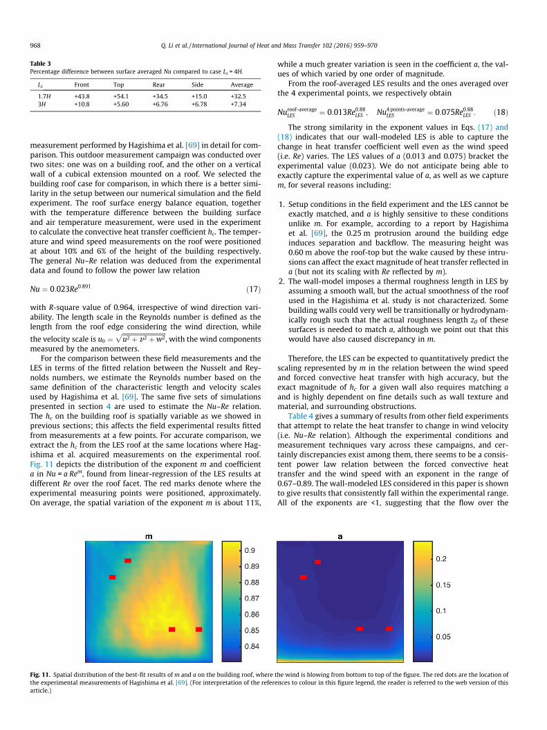
Table 3Percentage difference between surface averaged Nu compared to case Lz = 4H.

Lz Front Top Rear Side Average

1.7H +43.8 +54.1 +34.5 +15.0 +32.53H +10.8 +5.60 +6.76 +6.78 +7.34

968 Q. Li et al. / International Journal of Heat and Mass Transfer 102 (2016) 959–970

measurement performed by Hagishima et al. [69] in detail for com-parison. This outdoor measurement campaign was conducted overtwo sites: one was on a building roof, and the other on a verticalwall of a cubical extension mounted on a roof. We selected thebuilding roof case for comparison, in which there is a better simi-larity in the setup between our numerical simulation and the fieldexperiment. The roof surface energy balance equation, togetherwith the temperature difference between the building surfaceand air temperature measurement, were used in the experimentto calculate the convective heat transfer coefficient hc. The temper-ature and wind speed measurements on the roof were positionedat about 10% and 6% of the height of the building respectively.The general Nu–Re relation was deduced from the experimentaldata and found to follow the power law relation

Nu ¼ 0:023Re0:891 ð17Þ

with R-square value of 0.964, irrespective of wind direction vari-ability. The length scale in the Reynolds number is defined as thelength from the roof edge considering the wind direction, while

the velocity scale is u0 ¼ffiffiffiffiffiffiffiffiffiffiffiffiffiffiffiffiffiffiffiffiffiffiffiffiffiffiffiffiu2 þ v2 þw2

p, with the wind components

measured by the anemometers.For the comparison between these field measurements and the

LES in terms of the fitted relation between the Nusselt and Rey-nolds numbers, we estimate the Reynolds number based on thesame definition of the characteristic length and velocity scalesused by Hagishima et al. [69]. The same five sets of simulationspresented in section 4 are used to estimate the Nu–Re relation.The hc on the building roof is spatially variable as we showed inprevious sections; this affects the field experimental results fittedfrom measurements at a few points. For accurate comparison, weextract the hc from the LES roof at the same locations where Hag-ishima et al. acquired measurements on the experimental roof.Fig. 11 depicts the distribution of the exponent m and coefficienta in Nu = a Rem, found from linear-regression of the LES results atdifferent Re over the roof facet. The red marks denote where theexperimental measuring points were positioned, approximately.On average, the spatial variation of the exponent m is about 11%,

Fig. 11. Spatial distribution of the best-fit results of m and a on the building roof, where tthe experimental measurements of Hagishima et al. [69]. (For interpretation of the referearticle.)

while a much greater variation is seen in the coefficient a, the val-ues of which varied by one order of magnitude.

From the roof-averaged LES results and the ones averaged overthe 4 experimental points, we respectively obtain

Nuroof-averageLES ¼ 0:013Re0:88LES ; Nu4 points-average

LES ¼ 0:075Re0:88LES : ð18ÞThe strong similarity in the exponent values in Eqs. (17) and

(18) indicates that our wall-modeled LES is able to capture thechange in heat transfer coefficient well even as the wind speed(i.e. Re) varies. The LES values of a (0.013 and 0.075) bracket theexperimental value (0.023). We do not anticipate being able toexactly capture the experimental value of a, as well as we capturem, for several reasons including:

1. Setup conditions in the field experiment and the LES cannot beexactly matched, and a is highly sensitive to these conditionsunlike m. For example, according to a report by Hagishimaet al. [69], the 0.25 m protrusion around the building edgeinduces separation and backflow. The measuring height was0.60 m above the roof-top but the wake caused by these intru-sions can affect the exact magnitude of heat transfer reflected ina (but not its scaling with Re reflected by m).

2. The wall-model imposes a thermal roughness length in LES byassuming a smooth wall, but the actual smoothness of the roofused in the Hagishima et al. study is not characterized. Somebuilding walls could very well be transitionally or hydrodynam-ically rough such that the actual roughness length z0 of thesesurfaces is needed to match a, although we point out that thiswould have also caused discrepancy in m.

Therefore, the LES can be expected to quantitatively predict thescaling represented by m in the relation between the wind speedand forced convective heat transfer with high accuracy, but theexact magnitude of hc for a given wall also requires matching aand is highly dependent on fine details such as wall texture andmaterial, and surrounding obstructions.

Table 4 gives a summary of results from other field experimentsthat attempt to relate the heat transfer to change in wind velocity(i.e. Nu–Re relation). Although the experimental conditions andmeasurement techniques vary across these campaigns, and cer-tainly discrepancies exist among them, there seems to be a consis-tent power law relation between the forced convective heattransfer and the wind speed with an exponent in the range of0.67–0.89. The wall-modeled LES considered in this paper is shownto give results that consistently fall within the experimental range.All of the exponents are <1, suggesting that the flow over the

he wind is blowing from bottom to top of the figure. The red dots are the location ofnces to colour in this figure legend, the reader is referred to the web version of this

Table 4The exponent in the Nu–Re relation for different experiments and correspondingvalues from LES.

Experimental LES

Emmel et al. [30] 0.85 (Roof) 0.88Clear et al. [32] 0.8 (Roof) 0.88Yazdamian and Klems [31] 0.89 (Windward, low-rise building) 0.89

0.671 (Leeward, low-rise building) 0.90

Q. Li et al. / International Journal of Heat and Mass Transfer 102 (2016) 959–970 969

surfaces is not in the fully rough regime where the Stanton numberwould become independent of Re.

6. Discussion and conclusions

This study assessed the capability of the wall-modeled LESapproach to capture the physics of forced convective heat/masstransfer between the surfaces of buildings and the atmosphere.Through detailed comparisons to both wind-tunnel studies andfield experiment, we have shown that our LES is able to reasonablypredict (i) the spatial variation of the heat/mass transfer coefficientover the different facets of 2D ribs; (ii) the average Nusselt numberfor a single cube (with larger discrepancy relative to measurementsover the windward face very likely related to the Re discrepancy);and (iii) the power law relation between the Nusselt and Reynoldsnumbers compared to field measurements. The excellent match ofthe power law exponent m is largely attributable to the dynamicwall model we proposed and implemented here.

Returning to the motivating question we asked: ‘‘are the errorsresulting from the parameterization of unresolved scales (wall andsubgrid scale models) in LES larger or smaller than the errorsinvolved in extrapolating from low-Re approaches (DNS or windtunnels) to high-Re real world flows, for scalar transfer problems?”,the overall conclusion from out study indicates that the LES,despite its inherent parameterizations, is more suitable for study-ing real-world buildings:

1. Wind-tunnel studies result in Nu � Re0.52–0.74, a significantlylower exponent range than the �0.9 observed in field measure-ments and LES. This is consistent with the expected trend of alower m when Re is lower, and suggests that the low-Re effectsin the wind tunnel are biasing the findings and would makethem not suitable for extrapolation to the real-world (yet asmentioned in the introduction some current models rely onsuch coefficients empirically determined from water channelstudies from 1924 [14]). As such, when LES-wind tunnel dis-crepancies arise, it seem more likely that the errors are relatedto the extrapolation of wind tunnel Nu–Re relations outsidetheir range of validity.

2. There is a strong sensitivity of the heat transfer exchange coef-ficient to inflow conditions, and the inflow is wind tunnel stud-ies (or many simulations for that matter) do not representrealistic upwind conditions in the real world.

For building models and urban microclimate models that oftenuse averaged value for modeling turbulent heat exchange, based onour simulation results, the use of facet-averaged values seem to beappropriate, but the relatively large differences among differentfacets preclude the use of a single coefficient for the whole buildingsince this would not capture the large facet-to-facet variations. Inaddition, we have documented (not surprisingly) that it is impor-tant in numerical simulation like LES to match the experimentalinflow conditions, especially for the windward faces that areaffected the most. For future experimental studies in wind tunnelsor field experiments, details such as the inflow profiles in a windtunnel, measuring positions of wind and temperature, and wind

directions should be included so that further validation studiescan be conducted with more details of the experimental setup.For the types of numerical experiments considered here, the suit-able domain height should be greater than 4 times the height ofthe obstacle. Another point to note is that the exponent m inNu � Rem being close to 1.0 (both in building-scale field measure-ment and LES) is a manifestation of approaching the fully roughlimit [27], in which the Stanton number is independent of Re. How-ever, this limit is not reached suggesting that transitional effectspersist. This should not be confused with the building canopy scaleflow, which is clearly in the fully rough regime.

Going forward, the results gives us confidence in the capabilityof LES and the potential for using the technique to develop a betterunderstanding of coupled scalar and momentum transfer at high-Re over complex topographies, and to formulate improvedspatially-averaged surface exchange models to be used in coarseatmospheric models (weather or climate) where the buildings can-not be resolved.

Acknowledgement

This study was funded by the US National Science Foundation’sSustainability Research Network Cooperative Agreement #1444758 and Water Sustainability and Climate program Grant #CBET-1058027. The simulations were performed on the supercom-puting clusters of the National Center for Atmospheric Researchthrough project P36861020. W.A. was supported by the ArmyResearch Office Environmental Sciences Directorate (Grant #W911NF-15-1-0231; PM: Dr. J. Parker).

References

[1] M. Mirsadeghi, D. Cóstola, B. Blocken, J.L.M. Hensen, Review of externalconvective heat transfer coefficient models in building energy simulationprograms: implementation and uncertainty, Appl. Therm. Eng. 56 (2013) 134–151.

[2] T. Defraeye, B. Blocken, J. Carmeliet, Convective heat transfer coefficients forexterior building surfaces: existing correlations and CFD modelling, EnergyConvers. Manage. 52 (2011) 512–522, http://dx.doi.org/10.1016/j.enconman.2010.07.026.

[3] J.A. Palyvos, A survey of wind convection coefficient correlations for buildingenvelope energy systems’ modeling, Appl. Therm. Eng. 28 (2008) 801–808,http://dx.doi.org/10.1016/j.applthermaleng.2007.12.005.

[4] D. Li, E. Bou-Zeid, Quality and sensitivity of high-resolution numericalsimulation of urban heat islands, Environ. Res. Lett. 9 (2014).

[5] T.H. Chilton, A.P. Colburn, Mass transfer (absorption) coefficients predictionfrom data on heat transfer and fluid friction, Ind. Eng. Chem. 26 (1934) 1183–1187, http://dx.doi.org/10.1021/ie50299a012.

[6] B. Blocken, J. Carmeliet, The influence of the wind-blocking effect by a buildingon its wind-driven rain exposure, J. Wind Eng. Ind. Aerodyn. 94 (2006) 101–127.

[7] T. Sun, E. Bou-Zeid, Z.-H. Wang, E. Zerba, G.-H. Ni, Hydrometeorologicaldeterminants of green roof performance via a vertically-resolved model forheat and water transport, Build. Environ. 60 (2013) 211–224, http://dx.doi.org/10.1016/j.buildenv.2012.10.018.

[8] T. Sun, E. Bou-Zeid, G.-H. Ni, To irrigate or not to irrigate: analysis of green roofperformance via a vertically-resolved hygrothermal model, Build. Environ. 73(2014) 127–137, http://dx.doi.org/10.1016/j.buildenv.2013.12.004.

[9] V. Masson, A physically-based scheme for the urban energy budget inatmospheric models, Boundary Layer Meteorol. 94 (2000) 357–397, http://dx.doi.org/10.1023/A:1002463829265.

[10] Z.-H. Wang, E. Bou-Zeid, J.A. Smith, A coupled energy transport andhydrological model for urban canopies evaluated using a wireless sensornetwork, Q. J. R. Meteorol. Soc. 139 (2013) 1643–1657, http://dx.doi.org/10.1002/qj.2032.

[11] C.S.B. Grimmond, M. Blackett, M.J. Best, J.J. Baik, S.E. Belcher, J. Beringer, et al.,Initial results from Phase 2 of the international urban energy balance modelcomparison, Int. J. Climatol. 31 (2011) 244–272, http://dx.doi.org/10.1002/joc.2227.

[12] C.S.B. Grimmond, T.R. Oke, D.G. Steyn, Urban Water Balance 1. A Model forDaily Totals, 1986.

[13] A. Hagishima, J. Tanimoto, K.I. Narita, Intercomparisons of experimentalconvective heat transfer coefficients and mass transfer coefficients of urbansurfaces, Boundary Layer Meteorol. 117 (2005) 551–576.

[14] W. Jürges, Der Wärmeübergang an einer ebenen Wand, 1924.

970 Q. Li et al. / International Journal of Heat and Mass Transfer 102 (2016) 959–970

[15] I.P. Castro, H. Cheng, R. Reynolds, Turbulence over urban-type roughness:deductions from wind-tunnel measurements, Boundary Layer Meteorol. 118(2006) 109–131, http://dx.doi.org/10.1007/s10546-005-5747-7.

[16] J. Jiménez, Turbulent flows over rough walls, 36 (2004) 173–196, <http://Dx.Doi.org/10.1146/Annurev.Fluid.36.050802.122103>.

[17] D.A. Aliaga, J.P. Lamb, D.E. Klein, Convection heat transfer distributions overplates with square ribs from infrared thermography measurements, Int. J. HeatMass Transfer 37 (1994) 363–374, http://dx.doi.org/10.1016/0017-9310(94)90071-X.

[18] M.K. Chyu, V. Natarajan, Local heat/mass transfer distributions on the surfaceof a wall-mounted cube, Trans. ASME J. Heat Transfer 113 (1991) 851–857,http://dx.doi.org/10.1115/1.2911213.

[19] T. Igarashi, Heat transfer from a square prism to an air stream, Int. J. HeatMass Transfer 28 (1985) 175–181, http://dx.doi.org/10.1016/0017-9310(85)90019-5.

[20] E.R. Meinders, T.H. Van Der Meer, K. Hanjalic, Local convective heat transferfrom an array of wall-mounted cubes, Int. J. Heat Mass Transfer 41 (1998)335–346, http://dx.doi.org/10.1016/S0017-9310(97)00148-8.

[21] E.R. Meinders, K. Hanjalic, Vortex structure and heat transfer in turbulent flowover a wall-mounted matrix of cubes, Int. J. Heat Mass Transfer 20 (1999) 255–267, http://dx.doi.org/10.1016/S0142-727X(99)00016-8.

[22] H. Nakamura, T. Igarashi, T. Tsutsui, Local heat transfer around a wall-mountedcube in the turbulent boundary layer, Int. J. Heat Mass Transfer 44 (2001)3385–3395, http://dx.doi.org/10.1016/S0017-9310(01)00009-6.

[23] K.I. Narita, Experimental study of the transfer velocity for urban surfaces witha water evaporation method, Boundary Layer Meteorol. 122 (2007) 293–320.

[24] F. Pascheke, J.F. Barlow, A. Robins, Wind-tunnel modelling of dispersion from ascalar area source in urban-like roughness, Boundary Layer Meteorol. 126(2007) 103–124, http://dx.doi.org/10.1007/s10546-007-9222-5.

[25] J.F. Barlow, I.N. Harman, S.E. Belcher, Scalar fluxes from urban street canyons.Part I: laboratory simulation, Boundary Layer Meteorol. 113 (2004) 369–385,http://dx.doi.org/10.1007/s10546-004-6204-8.

[26] J.H. Lienhard, A Heat Transfer Textbook, Courier Corporation, 2013.[27] R.L. Webb, E.R.G. Eckert, R.J. Goldstein, Heat transfer and friction in tubes with

repeated-rib roughness, Int. J. Heat Mass Transfer 14 (1971) 601–617, http://dx.doi.org/10.1016/0017-9310(71)90009-3.

[28] F.L. Test, R.C. Lessmann, A. Johary, Heat transfer during wind flow overrectangular bodies in the natural environment, Trans. ASME J. Heat Transfer103 (1981) 262–267, http://dx.doi.org/10.1115/1.3244451.

[29] D.L. Loveday, A.H. Taki, Convective heat transfer coefficients at a plane surfaceon a full-scale building facade, Int. J. Heat Mass Transfer 39 (1996) 1729–1742,http://dx.doi.org/10.1016/0017-9310(95)00268-5.

[30] M.G. Emmel, M.O. Abadie, N. Mendes, New external convective heat transfercoefficient correlations for isolated low-rise buildings, Energy Build. 39 (2007)335–342.

[31] M. Yazdanian, J.H. Klems, Measurement of the exterior convective filmcoefficient for windows in low-rise buildings, ASHRAE Trans. 100 (1994)1087–1096.

[32] R.D. Clear, L. Gartland, F.C. Winkelmann, An empirical correlation for theoutside convective air-film coefficient for horizontal roofs, Energy Build. 35(2003) 797–811.

[33] Y. Liu, D.J. Harris, Full-scale measurements of convective coefficient onexternal surface of a low-rise building in sheltered conditions, Build.Environ. 42 (2007) 2718–2736.

[34] S.B. Park, J.J. Baik, A large-eddy simulation study of thermal effects onturbulence coherent structures in and above a building array, J. Appl. Meteorol.Climatol. 52 (2013) 1348–1365.

[35] V.B.L. Boppana, Z.-T. Xie, I.P. Castro, Large-eddy simulation of heat transferfrom a single cube mounted on a very rough wall, Boundary Layer Meteorol.147 (2012) 347–368, http://dx.doi.org/10.1007/s10546-012-9793-7.

[36] T. Defraeye, B. Blocken, J. Carmeliet, CFD simulation of heat transfer at surfacesof bluff bodies in turbulent boundary layers: evaluation of a forced-convectivetemperature wall function for mixed convection, J. Wind Eng. Ind. Aerodyn.104–106 (2012) 439–446.

[37] J. Liu, J. Srebric, N. Yu, Numerical simulation of convective heat transfercoefficients at the external surfaces of building arrays immersed in a turbulentboundary layer, Int. J. Heat Mass Transfer 61 (2013) 209–225, http://dx.doi.org/10.1016/j.ijheatmasstransfer.2013.02.005.

[38] S. Leonardi, P. Orlandi, R.J. Smalley, L. Djenidi, R.A. Antonia, Direct numericalsimulations of turbulent channel flow with transverse square bars on one wall,J. Fluid Mech. 491 (2003) 229–238.

[39] S. Leonardi, L. Djenidi, P. Orlandi, R.A. Antonia, Heat transfer in a turublentchannel flow with square bars and circular rods on one wall, J. Fluid Mech. 776(2015) 512–530.

[40] O. Coceal, T.G. Thomas, I.P. Castro, S.E. Belcher, Mean flow and turbulencestatistics over groups of urban-like cubical obstacles, Boundary LayerMeteorol. 121 (2006) 491–519, http://dx.doi.org/10.1007/s10546-006-9076-2.

[41] O. Coceal, T.G. Thomas, S.E. Belcher, Spatial variability of flow statistics withinregular building arrays, Boundary Layer Meteorol. 125 (2007) 537–552, http://dx.doi.org/10.1007/s10546-007-9206-5.

[42] S.B. Pope, Turbulent Flows, Cambridge University Press, 2000.[43] D.B. Spalding, A new analytical expression for the drag of a flat plate valid for

both the turbulent and laminar regimes, Int. J. Heat Mass Transfer 5 (1962)1133–1138, http://dx.doi.org/10.1016/0017-9310(62)90189-8.

[44] C.H. Liu, T.N.H. Chung, Forced convective heat transfer over ribs at variousseparation, Int. J. Heat Mass Transfer 55 (2012) 5111–5119, http://dx.doi.org/10.1016/j.ijheatmasstransfer.2012.05.012.

[45] M.G. Giometto, A. Christen, C. Meneveau, J. Fang, M. Krafczyk, M.B. Parlange,Spatial characteristics of roughness sublayer mean flow and turbulence over arealistic urban surface, Boundary Layer Meteorol. (2016) 1–28, http://dx.doi.org/10.1007/s10546-016-0157-6.

[46] B.E. Launder, On the computation of convective heat-transfer in complexturbulent flows, J. Heat Transfer Trans. ASME 110 (1988) 1112–1128.

[47] J.C. Wyngaard, L.J. Peltier, S. Khanna, LES in the surface layer: surface fluxes,scaling, and SGS modeling, J. Atmos. Sci. 55 (1998) 1733–1754, http://dx.doi.org/10.1175/1520-0469(1998) 055<1733:LITSLS>2.0.CO;2.

[48] W. Cabot, P. Moin, Approximate wall boundary conditions in the large-eddysimulation of high Reynolds number flow, Flow Turbul. Combust. 63 (2000)269–291, http://dx.doi.org/10.1023/A:1009958917113.

[49] X.I.A. Yang, J. Sadique, R. Mittal, C. Meneveau, Integral wall model for largeeddy simulations of wall-bounded turbulent flows, Phys. Fluids (1994-Present) 27 (2015) 025112, http://dx.doi.org/10.1063/1.4908072.

[50] X. Yang, J. Sadique, R. Mittal, C. Meneveau, Exponential roughness layer andanalytical model for turbulent boundary layer flow over rectangular-prismroughness elements, J. Fluid Mech. 789 (2016) 127–165.

[51] T. Defraeye, B. Blocken, J. Carmeliet, An adjusted temperature wall function forturbulent forced convective heat transfer for bluff bodies in the atmosphericboundary layer, Build. Environ. 46 (2011) 2130–2141, http://dx.doi.org/10.1016/j.buildenv.2011.04.013.

[52] S.B. Pope, Ten questions concerning the large-eddy simulation of turbulentflows, New J. Phys. 6 (2004) 35, http://dx.doi.org/10.1088/1367-2630/6/1/035.

[53] J. Slotnick, CFD Vision 2030 Study, 2014.[54] S. Chester, C. Meneveau, M.B. Parlange, Modeling turbulent flow over fractal

trees with renormalized numerical simulation, J. Comput. Phys. 225 (2007)427–448, http://dx.doi.org/10.1016/j.jcp.2006.12.009.

[55] Y.H. Tseng, C. Meneveau, M.B. Parlange, Modeling flow around bluff bodies andpredicting urban dispersion using large eddy simulation, Environ. Sci. Technol.40 (2006) 2653–2662, http://dx.doi.org/10.1021/es051708m.

[56] V. Kumar, J. Kleissl, C. Meneveau, M.B. Parlange, Large-eddy simulation of adiurnal cycle of the atmospheric boundary layer: Atmospheric stability andscaling issues, Water Resour. Res. 42 (2006), http://dx.doi.org/10.1029/2005WR004651.

[57] S. Shah, E. Bou-Zeid, Very-large-scale motions in the atmospheric boundarylayer educed by snapshot proper orthogonal decomposition, Boundary LayerMeteorol. 153 (2014) 355–387, http://dx.doi.org/10.1007/s10546-014-9950-2.

[58] Q. Li, E. Bou-Zeid, W. Anderson, The impact and treatment of the Gibbsphenomenon in immersed boundary method simulations of momentum andscalar transport, J. Comput. Phys. 310 (2016) 237–251.

[59] E. Bou-Zeid, C. Meneveau, M. Parlange, A scale-dependent Lagrangian dynamicmodel for large eddy simulation of complex turbulent flows, Phys. Fluids 17(2005), http://dx.doi.org/10.1063/1.1839152.

[60] W. Anderson, Passive scalar roughness lengths for atmospheric boundary layerflow over complex, fractal topographies, Environ. Fluid Mech. 13 (2013) 479–501, http://dx.doi.org/10.1007/s10652-013-9272-9.

[61] B.A. Kader, A.M. Yaglom, Heat and mass transfer laws for fully turbulent wallflows, Int. J. Heat Mass Transfer 15 (1972) 2329–2351, http://dx.doi.org/10.1016/0017-9310(72)90131-7.

[62] A.E. Perry, J.B. Bell, P.N. Joubert, Velocity and temperature profiles in adversepressure gradient turbulent boundary layers, J. Fluid Mech. 25 (1966) 299–320, http://dx.doi.org/10.1017/S0022112066001666.

[63] L. Temmerman, M.A. Leschziner, C.P. Mellen, J. Fröhlich, Investigation of wall-function approximations and subgrid-scale models in large eddy simulation ofseparated flow in a channel with streamwise periodic constrictions, Int. J. HeatMass Transfer 24 (2003) 157–180, http://dx.doi.org/10.1016/S0142-727X(02)00222-9.

[64] T.R. Oke, Boundary Layer Climates, Routledge, 1978.[65] A.E. Perry, W.H. Schofield, P.N. Joubert, Rough wall turbulent boundary layers,

J. Fluid Mech. 37 (1969) 383–413, http://dx.doi.org/10.1017/S0022112069000619.

[66] S. Leonardi, I.P. Castro, Journal of Fluid Mechanics – Abstra ct – Channel flowover large cube roughness: a direct numerical simulation study, J. Fluid Mech.(2010).

[67] R. Martinuzzi, C. Tropea, The flow around surface-mounted, prismaticobstacles placed in a fully developed channel flow (data bank contribution),J. Fluids Eng. 115 (1993) 85–92, http://dx.doi.org/10.1115/1.2910118.

[68] F.P. Incropera, Introduction to Heat Transfer Fourth Edition Wie, Wiley, 2002.[69] A. Hagishima, J. Tanimoto, Field measurements for estimating the convective

heat transfer coefficient at building surfaces, Build. Environ. 38 (2003) 873–881, http://dx.doi.org/10.1016/S0360-1323(03)00033-7.