international journal of control - university of...

This article was downloaded by: [University of Michigan]On: 17 September 2012, At: 13:01Publisher: Taylor & FrancisInforma Ltd Registered in England and Wales Registered Number: 1072954 Registered office: Mortimer House,37-41 Mortimer Street, London W1T 3JH, UK

International Journal of ControlPublication details, including instructions for authors and subscription information:http://www.tandfonline.com/loi/tcon20

Assessment of non-centralised model predictivecontrol techniques for electrical power networksRalph M. Hermans a , Andrej Jokić a , Mircea Lazar a , Alessandro Alessio b , Paul P.J. van

den Bosch a , Ian A. Hiskens c & Alberto Bemporad da Department of Electrical Engineering, Eindhoven University of Technology, P.O. Box 513,Eindhoven, 5600 MB Netherlandsb Department of Information Engineering, University of Siena, Siena, Italyc Department of Electrical Engineering and Computer Science, University of Michigan, AnnArbor, MI, USAd IMT Institute for Advanced Studies Lucca, Lucca, Italy

Version of record first published: 20 Apr 2012.

To cite this article: Ralph M. Hermans, Andrej Jokić, Mircea Lazar, Alessandro Alessio, Paul P.J. van den Bosch, Ian A.Hiskens & Alberto Bemporad (2012): Assessment of non-centralised model predictive control techniques for electrical powernetworks, International Journal of Control, 85:8, 1162-1177

To link to this article: http://dx.doi.org/10.1080/00207179.2012.679972

PLEASE SCROLL DOWN FOR ARTICLE

Full terms and conditions of use: http://www.tandfonline.com/page/terms-and-conditions

This article may be used for research, teaching, and private study purposes. Any substantial or systematicreproduction, redistribution, reselling, loan, sub-licensing, systematic supply, or distribution in any form toanyone is expressly forbidden.

The publisher does not give any warranty express or implied or make any representation that the contentswill be complete or accurate or up to date. The accuracy of any instructions, formulae, and drug doses shouldbe independently verified with primary sources. The publisher shall not be liable for any loss, actions, claims,proceedings, demand, or costs or damages whatsoever or howsoever caused arising directly or indirectly inconnection with or arising out of the use of this material.

http://www.tandfonline.com/loi/tcon20

http://dx.doi.org/10.1080/00207179.2012.679972

http://www.tandfonline.com/page/terms-and-conditions

International Journal of ControlVol. 85, No. 8, August 2012, 1162–1177

Assessment of non-centralised model predictive control techniques for

electrical power networks

Ralph M. Hermansa*, Andrej Jokica, Mircea Lazara, Alessandro Alessiob, Paul P.J. van den Boscha,Ian A. Hiskensc and Alberto Bemporadd

aDepartment of Electrical Engineering, Eindhoven University of Technology, P.O. Box 513, Eindhoven,5600 MB Netherlands; bDepartment of Information Engineering, University of Siena, Siena, Italy;

cDepartment of Electrical Engineering and Computer Science, University of Michigan, Ann Arbor, MI, USA;dIMT Institute for Advanced Studies Lucca, Lucca, Italy

(Received 11 November 2011; final version received 23 March 2012)

Model predictive control (MPC) is one of the few advanced control methodologies that have proven to be verysuccessful in real-life applications. An attractive feature of MPC is its capability of explicitly taking state andinput constraints into account. Recently, there has been an increasing interest in the usage of MPC schemes tocontrol electrical power networks. The major obstacle for implementation lies in the large scale of these systems,which is prohibitive for a centralised approach. In this article, we therefore assess and compare the suitability ofseveral non-centralised predictive control schemes for power balancing, to provide valuable insights that cancontribute to the successful implementation of non-centralised MPC in the real-life electrical power system.

Keywords: model predictive control; decentralised control; distributed control; power systems

1. Introduction

Electrical power networks are among the largest and

most complex-engineered systems ever created. In spite

of their immense complexity, power systems have

shown an impressive level of performance and robust-

ness. One reason for their success is that traditional

power systems are characterised by a highly repetitive

daily pattern of power flows, with a relatively small

amount of suddenly occurring, uncertain fluctuations

on the demand side, and with controllable, large power

plants on the supply side. As a consequence, in

traditional power systems, a large portion of energy

production can be efficiently scheduled in an open-

loop manner, with automatic generation control

(AGC) (Jaleeli, VanSlyck, Ewart, Fink, and

Hoffmann 1992; Kundur 1994) providing efficient

real-time power balancing of uncertain demands.However, today, electrical power systems are

undergoing two fundamental restructuring processes.

Firstly, from a regulated, single-utility controlled

operation, the system has been restructured to include

many parties that compete for power production and

consumption (see, e.g. Stoft (2002) and the references

therein). With power markets as the central opera-

tional mechanism, competitive economic forces often

push the system towards its operational boundaries.

Secondly, there has been an increasing integration ofsmall-scale distributed generation (DG), see, e.g.Borbely and Kreider (2001) and the references therein.Since large amounts of DG are expected to be based onrenewable, intermittent energy sources, such as windand sun, future power systems will be characterised bylarge and unpredictable power fluctuations on thepower production side. These observations lead to theconclusion that the preservation of the high perfor-mance and robustness levels that were attained in thepast will become a major challenge for power systemcontrol in the near future.

Various recent papers have observed that modelpredictive control (MPC) has the potential for solvingthe problems that will appear in future electrical powernetworks (Camponogara 2000; Camponogara, Jia,Krogh, and Talukdar 2002; Venkat 2006; Jokic,Lazar, and Van den Bosch 2007; Venkat, Hiskens,Rawlings, and Wright 2008). MPC is capable ofhandling control problems where off-line computationof a classical control law is difficult, particularly sinceMPC can explicitly take system constraints intoaccount when computing the control action.Furthermore, MPC allows the use of disturbancemodels, which can be employed to counteract thefluctuations in power generation introduced by renew-able energy sources. For a detailed survey of MPC and

*Corresponding author. Email: [email protected]

ISSN 0020–7179 print/ISSN 1366–5820 online

� 2012 Taylor & Francis

http://dx.doi.org/10.1080/00207179.2012.679972

http://www.tandfonline.com

Dow

nloa

ded

by [

Uni

vers

ity o

f M

ichi

gan]

at 1

3:01

17

Sept

embe

r 20

12

constrained optimal control, the interested reader isreferred to Mayne, Rawlings, Rao, and Scokaert(2000) and Goodwin, Seron, and De Dona (2005).

Yet, the fact that MPC is a centralised controlmechanism is a major issue when considering powersystem operation. Centralised control implies that asingle controller is able to measure all the systemoutputs, compute the optimal control solution,and apply that action to all actuators in the network,within one sampling period. As power networksare large-scale systems, both computationally andgeographically, a centralised MPC controller is practi-cally impossible to implement.

The difficulties with centralised predictive controlfor large-scale systems explain the increasing attentionfor non-centralised MPC implementations in thecontrol literature (see, for example Camponogara2000; Camponogara et al. 2002; Keviczky,Borrelli, and Balas 2006; Alessio and Bemporad2007; Dunbar 2007; Venkat et al. 2008). Roughlyspeaking, non-centralised MPC schemes can be dividedinto two categories: decentralised techniques, whichdo not allow for communication between localcontrollers and distributed techniques, where commu-nication between different controllers is exploitedto improve the prediction accuracy. Distributed MPCmethods can be further categorised as techniquesthat require communication between all thecontrollers in the network and techniques that requirecommunication solely with directly neighbouringcontrollers.

In the literature on non-centralised predictivecontrol, various power system implementations havebeen illustrated, (Camponogara 2000; Camponogaraet al. 2002; Venkat et al. 2008). These methods differ interms of computational complexity, the extent ofcommunication and the size of the embedded predic-tion model, and, as a consequence, in terms ofperformance. In this article, we consider decentralisedMPC (DMPC; Alessio and Bemporad 2007), stability-constrained distributed MPC (SC-DMPC;Camponogara et al. 2002) and feasible cooperation-based MPC (FC-MPC; Venkat 2006), all of whichrepresent viable candidates for implementation inpower systems. Alternative methods, such as strategiesfor enforcing constraints that involve the dynamics ofmultiple control areas (see for instance, Keviczky et al.(2006), Richards and How (2007)) are not discussed, asthe literature does not yet give a solid solution fordealing with coupled constraints in a low-complexityand non-conservative fashion. For a discussion on thetheoretical issues regarding non-centralised MPCin general, the interested reader is referred to(Camponogara 2000; Camponogara et al. 2002;Keviczky et al. 2006; Alessio and Bemporad 2007;

Dunbar 2007; Richards and How 2007; Venkat et al.2008) and the references therein.

The choice for DMPC, SC-DMPC and FC-MPC isfurther motivated by our main research goal, which isto study the correlation between the complexity andusefulness of non-centralised MPC schemes and theircorresponding attainable performance. DMPC doesnot require communication and therefore belongs tothe decentralised and simplest category of non-centralised MPC. Although, specific implementationsof DMPC do exploit an exchange of informationbetween controllers, we will only consider the com-pletely decentralised version in this article, to give anindication of the performance that can be obtainedwithout communication. SC-DMPC and FC-MPC aredistributed MPC schemes, as they both employcommunication to increase the accuracy of their statepredictions. The FC-MPC technique requires commu-nication between all local controllers and uses aniterative procedure to compute the control action,while the SC-DMPC scheme requires communicationbetween directly neighbouring subsystems only. Assuch, SC-DMPC can be viewed as the outcome of atrade-off between the complexity and performanceattainable by DMPC on the one hand, and FC-MPCon the other.

The remainder of this article is organised asfollows. Section 2 introduces the (centralised) MPCmethodology along with the conditions that arenecessary to guarantee closed-loop stability. InSection 3, we describe the non-centralised MPCtechniques from an engineering perspective, particu-larly focusing on the details relevant for controllerimplementation. Section 4 contains a simulation studyof the MPC algorithms under consideration, which isbased on a suitably constructed power networkexample. The non-centralised MPC schemes arecompared with centralised MPC and with the classicalAGC method that is currently employed in real-lifepower system control. Given the results of thisbenchmark test, we discuss the suitability of theconsidered methods for balancing/frequency controlin power networks. We finish by listing the mainconclusions in Section 5.

1.1 Nomenclature

LetR,Z and Zþ denote the field of real numbers, the setof integers and the set of non-negative integers,respectively. For an arbitrary sequence u¼ (u(0),u(1), . . .), we use the notation u[k] to denote thetruncation of u at k2Zþ, i.e. u[k] :¼ (u(0),u(1), . . . , u(k)) with k� 1. The operator col(�, . . . , �)stacks its operands into a column vector and

International Journal of Control 1163

Dow

nloa

ded

by [

Uni

vers

ity o

f M

ichi

gan]

at 1

3:01

17

Sept

embe

r 20

12

diag(M1, . . . ,Mn) denotes a block diagonal matrix withmatricesMi on the main diagonal. The notations A�BandA�B denote thatA andB are Hermitian andA�Bis positive definite or positive semi-definite, respectively.

2. Centralised MPC

The basic principles of MPC are illustrated in Figure 1.In MPC, the control action is computed by solving afinite-horizon open-loop optimal control problem ateach sampling instant. The controller employs a modelto obtain a prediction of the state evolution over time,given the current state of the controlled system. Onlythe first sample of the optimising input sequence isapplied to the plant, after which the whole process isrepeated at the next time instant. This is the maindifference with classical control, which commonly usesa pre-computed and fixed feedback law. The unique,distinguishing feature of MPC lies in its ability tocompute the control input while explicitly taking inputand state constraints into account.

In this article, we consider systems that can beaccurately modelled using linear discrete-time state-space representations of the form

xðtþ 1Þ ¼ AxðtÞ þ BuðtÞ, ð1Þ

where A2Rn�n, B2R

n�m, x(t)2Rn is the state

and u(t)2Rm is the control input at discrete-time

instant t2Zþ. Note that the number of states n inpower networks that consist of thousands of nodes/buses can be very large, which corresponds to high-dimensional A and B matrices.

Let the control input and the predicted state at time

instants tþ k2Zþ, given x(t), be denoted by �u(k)

and �xðkÞ, respectively. Moreover, let �u[N�1]¼ ( �u(0),

. . . , �u(N� 1)) be a sequence of control moves, where

N2Zþ is the prediction horizon. The optimal control

problem that the MPC controller solves each sampling

instant, is formally defined as follows.

Problem 2.1: At discrete-time instant t2Zþ let x(t)

and N� 1 be given, set �xð0Þ :¼ xðtÞ and solve

V�NðxÞ ¼ min�u½N�1fVNðx, �u½N�1Þ j �u½N�1 2 UNðxÞg, ð2aÞ

where

VNðx, �u½N�1Þ ¼ Fð �xðNÞÞ þXN�1k¼0

‘ ð �xðkÞ, �uðkÞÞ

¼ �x>ðNÞP �xðNÞ

þXN�1k¼0

�x>ðkÞQ �xðkÞ þ �u>ðkÞR �uðkÞ ð2bÞ

�xðkþ 1Þ ¼ A �xðkÞ þ B �uðkÞ, ð2cÞ

for k¼ 0, . . . ,N� 1.

The matrices Q¼Q>� 0 and R¼R>� 0 are

suitably chosen performance weights, i.e. tuning

parameters, whereas the matrix P¼P>� 0 that

weights the terminal state is usually computed off-line

in such a way that closed-loop stability is guaranteed

(Mayne et al. 2000).

Figure 1. A schematic illustration of model predictive control.

1164 R.M. Hermans et al.

Dow

nloa

ded

by [

Uni

vers

ity o

f M

ichi

gan]

at 1

3:01

17

Sept

embe

r 20

12

The control problem defined by (2a) minimises thequadratic cost function VN(x, �u[N�1]) over all inputsequences �u[N�1] in the set UN(x). We assume thatUN(x) can be defined by a finite number of linearinequalities on u, such that the MPC optimisationproblem can be formulated as a quadratic program(QP). The set of feasible input sequences is determinedby the constraints on the states and inputs,

UNðxÞ :¼�

�u½N�1 2 UNj �xðkÞ 2 X,

k ¼ 1, . . . ,N� 1, �xðNÞ 2 Xf

�, ð3Þ

where UN :¼U� � � ��U is the N-times Cartesian

product of U. The set of feasible inputs U is a compactsubset of R

m and X is a closed subset of Rn.

Asymptotic stability of the MPC-controlled systemcan be guaranteed a priori by constraining the terminalstate �xðNÞ to an appropriately chosen terminal setXfX and by using a specific terminal weight P(Mayne et al. 2000). The set Xf must be positivelyinvariant (see Blanchini (1994)) and should satisfy thefollowing property:

Xf O1 :¼�x 2 R

nj KðAþ BK Þkx 2 U

and ðAþ BK Þkx 2 X, k ¼ 0, . . . ,1�, ð4Þ

where the pair {P,K } is obtained as the solution of theunconstrained infinite horizon LQR problem (Mayneet al. 2000), i.e.

P ¼ ðAþ BK Þ>PðAþ BK Þ þ K>RKþQ, ð5aÞ

K ¼ �ðRþ B>PBÞ�1B>PA: ð5bÞ

After solving Problem 2.1, the controller applies thefirst element of the optimal input sequence �u�½N�1 tothe system, i.e. u(t) :¼ �u*(0), and discards the rest of thesequence. At the next time instant, the state of thesystem is measured and the procedure described aboveis repeated. This so-called receding horizon strategyintroduces a closed-loop feedback mechanism toincrease robustness.

3. Non-centralised MPC

As explained in Section 1, a centralised implementationof MPC is not well-suited for control of powernetworks due to the complexity and size of thesesystems. In this section, we describe three less complexnon-centralised MPC techniques that are more appro-priate for power system control. We start by introdu-cing the basic notions and definitions used in thedescription of these algorithms.

Consider a power network that is represented bythe directed graph G¼ (S, E), with a finite number of

vertices S ¼ {&1, . . . , &M} and a set of directed edgesE {(&i, &j)2S �S j i 6¼ j}. We can model the dynamicsof the power network by assigning a dynamical systemto each vertex &i2S, with the dynamics governed by,

xiðkþ 1Þ ¼ fiðxiðkÞ, uiðkÞ, viðxN iðkÞÞÞ, ð6Þ

for k2Zþ and i2I :¼ {1, . . . ,M}. Here, xi 2 Xi Rni ,

ui 2 Ui Rmi are the state and control input of the ith

subsystem. We assume that the feasible input and statesets, Ui and Xi respectively, are polytopic, such thatthey can be described by a finite number of affineinequalities. With each edge (&i, &j)2E, we associate afunction vij : R

nj ! Rni that defines the interconnection

signal vij(xj(k)) between subsystem j and i. We useN i :¼ {j j (&i, &j)2E} to denote the set of indicescorresponding to the neighbours of subsystem i. Theterm neighbour of system i defines any system inthe network whose dynamics appear explicitly (via thefunction vij(�)) in the state equation that describes thedynamics of subsystem i. If system j is a neighbourof system i, in general this does not necessarily implythe reverse. Moreover, let xN i

ðkÞ :¼ colðfxj ðkÞgj2N iÞ

be the vector that collects all the state vectors ofthe neighbours of system i and viðxN i

Þ :¼colðfvijðxj ðkÞÞÞgj2N i

Þ be the vector-valued interconnec-tion signals that enter system i.

3.1 Decentralised MPC

The DMPC technique (Alessio and Bemporad 2007)exploits the fact that many large-scale systems, such aspower networks, consist of several subsystems (orcontrol areas) that are only loosely coupled. As aconsequence, these systems can be modelled by sparsestate-space representations. In DMPC, the globalstate-space model is approximated via a state andinput matrix partitioning that defines a set of Mdecoupled prediction models. Correspondingly, theDMPC controller equals the ensemble of M localMPC controllers that are independently designed foreach subsystem.

Let the large-scale system that is to be controlled bedescribed by the discrete-time state-space model givenin (1). The division into M subsystems employed inDMPC is based on an explicit transformationvia suitably defined matrices Wi and Zi, i2I :¼{1, . . . ,M}. These matrices collect the states andinputs assigned to subsystem i:

xi ¼W>i x, ui ¼ Z>i u, ð7aÞ

where xi 2 Rni and ui 2 R

mi . The corresponding local,decoupled prediction models are given by

�xiðkþ 1Þ ¼ Ai �xiðkÞ þ Bi �uiðkÞ ð7bÞ


Dow

nloa

ded

by [

Uni

vers

ity o

f M

ichi

gan]

at 1

3:01

17

Sept

embe

r 20

12

Ai ¼W>i AWi, Bi ¼W>i BZi, ð7cÞ

for i2I , where Ai 2 Rni�ni , Bi 2 R

ni�mi .Note that Wi and Zi are such that, by (7a), each

element of x is assigned to one or more xi and each

element of u is assigned to one or more ui. This means

that overlapping subsystems are allowed. However, in

this article, we will consider DMPC with non-over-

lapping partitions only, i.e. we restrict our attention to

the cases where each element of x is assigned to a

unique xi and each element of u is assigned to a unique

ui. Although DMPC performance is expected to

improve with increasing subsystem overlap, the use

of non-overlapping partitions is attractive as this

requires no communication between subsystems. For

more information about the construction of the

partitioning matrices, and for details on handling

overlapping inputs in particular, the reader is referred

to Alessio and Bemporad (2007).In contrast to centralised MPC, the DMPC control

scheme assigns a controller to each subsystem i, which

solves the following finite-horizon problem, at each

sampling instant:

Problem 3.1 (DMPC): At discrete-time instant t2Zþ

let xi(t) and N� 1 be given, set �xið0Þ :¼ xiðtÞ and solve

V�i,NðxiÞ ¼ min�ui, ½N�1fVi,Nðxi, �ui, ½N�1Þ j �ui, ½N�1 2 Ui,NðxiÞg,

ð8aÞ

where

Vi,Nðxi, �ui, ½N�1Þ

¼ Fið �xiðNÞÞ þXN�1k¼0

‘ið �xiðkÞ, �uiðkÞÞ

¼ �x>i ðNÞPi �xiðNÞ

þXN�1k¼0

�x>i ðkÞQi �xiðkÞ þ �u>i ðkÞRi �uiðkÞ ð8bÞ

�xiðkþ 1Þ ¼ Ai �xiðkÞ þ Bi �uiðkÞ, k ¼ 0, . . . ,N� 1,

ð8cÞ

where the penalty matrices used in each cost function,

given the weights of a centralised controller, are Qi ¼

W>i QWi ¼ Q>i � 0, Ri ¼ Z>i RZi ¼ R>i � 0 and Pi,

which will be specified below.

Problem 3.1 minimises the local quadratic cost over

input sequences in the set

Ui,NðxiÞ :¼ f�ui, ½N�1 2 UNi g, ð9Þ

where UNi :¼ Ui � � � � �Ui is the N-times Cartesian

product of the set of feasible local inputs. We assume

that Ui,N is a polytope, i.e. it can be described by a

finite number of affine inequalities, such that we canformulate Problem 3.1 as a QP.

When all M controllers have calculated the optimallocal control action sequence �u�i, ½N�1, the ensemble ofall local inputs, i.e.

uðtÞ ¼ colð �u�1ð0Þ, . . . , �u�i ð0Þ, . . . , �u�Mð0ÞÞ, ð10Þ

is applied to the global system (1) and the wholeprocedure is repeated at the next time instant.

Unlike centralised MPC, the DMPC algorithmdoes not take (coupled) state constraints into account.However, note that in the case of frequency control inpower networks, state constraints such as bounds ontie-line flows can be essential to guarantee safeoperation.

Moreover, as described in Section 2, one canspecifically design centralised MPC to provide an apriori guarantee for closed-loop stability, based on aterminal penalty and terminal state conditions.However, these conditions only apply in the case ofcentralised MPC. Non-centralised predictive control-lers, such as DMPC, exploit modified stabilisationconditions, that possibly yield a weaker guarantee forclosed-loop stability. In DMPC, an a priori guaranteeof stability for each decoupled subsystem can beobtained by defining the terminal penalty matrix Pi

for each subsystem i as

Pi ¼ ðAi þ BiKiÞ>PiðAi þ BiKiÞ þ K>i RiKi þQi,

ð11aÞ

Ki ¼ �ðRi þ B>i PiBiÞ�1B>i PiAi, ð11bÞ

and constraining the terminal state �xiðNÞ to aninvariant (polytopic) terminal set

Xfi fx 2 Rni j KiðAi þ BiKiÞ

kx 2 Ui

and ðAi þ BiKiÞkx 2 Xi, k ¼ 0, . . . ,1g, ð12Þ

where Xi is the set of feasible local states. If Ki� 0, asin Alessio and Bemporad (2007), then (11a) reduces tothe Lyapunov equation. Note that because Qi� 0, thisimplies that each subsystem has to be open-loop stable,i.e. that all eigenvalues of Ai must be within the unitcircle.

Nonetheless, observe that condition (11) onlyimplies closed-loop stability under the assumptionthat the subsystems are indeed decoupled. Still, it ispossible to provide a posteriori verifiable stabilityconditions for the network under coupled operation,as shown in Alessio and Bemporad (2007). Moreprecisely, the proposed stability test checks stability ofthe entire system (1) in closed loop with (10), if thematrices Pi are chosen according to (11a). This aposteriori stability test checks whether the sum of all


Dow

nloa

ded

by [

Uni

vers

ity o

f M

ichi

gan]

at 1

3:01

17

Sept

embe

r 20

12

cost functions is a Lyapunov function for the overall

system, and is based on the explicit form of each MPC

controller (Bemporad, Morari, Dua, and Pistikopoulos2002). Under certain conditions, this reduces to a

positive semi-definiteness check of a square n� n

matrix. However, this test has to be carried out on acentralised level, which partly cancels out the attractive

features of DMPC’s decentralised structure.The main attractive feature of the DMPC scheme is

that each local controller has to solve relatively small

and simple optimisation problems, corresponding tolow computational requirements per subsystem.

However, it is important to observe that the DMPC

cost function of subsystem i solely depends on the localstates and inputs xi(t) and �ui,[N�1], respectively. This is

a consequence of the fact that the DMPC prediction

model (7) approximates the real system by ignoring thedynamic coupling between subsystems and uses only

local state information to initialise the optimisationproblem. Therefore, (10) will, in general, not be

optimal with respect to the centralised MPC optimisa-

tion problem (2) unless x� xi and u� ui, for all i. If thedynamic coupling between the subsystems in (1) is

strong, the prediction mismatch can be large, resultingin a significant loss of performance compared with that

attained by a centralised controller.

3.2 Stability-constrained distributed MPC

The SC-DMPC scheme (Camponogara et al. 2002) is adistributed predictive control method, in which each

local controller exploits communication with neigh-bouring subsystems to improve the accuracy of its local

state predictions. As such, SC-DMPC is expected to

outperform decentralised control schemes that neglectdynamic coupling and that do not exploit communica-

tion at all.The SC-DMPC scheme requires that the dynamics

of the system to be controlled are given by (1), with

state-space matrices that have the structure:

A ¼

A11 . . . A1M

..

. . .. ..

.

AM1 . . . AMM

264

375, B ¼

B11 . . . 0

..

. . .. ..

.

0 . . . BMM

264

375,

ð13Þ

where A2Rn�n, B2R

n�m, Aii 2 Rni�ni , Aij 2 R

ni�nj ,Bii 2 R

ni�mi , x2Rn and u2R

m. Note that B is block

diagonal, such that input ui only affects subsystem i

directly. Correspondingly, the neighbours of subsystemi are those systems for which Aij 6¼ 0, j 6¼ i. The set of

neighbours of system i is denoted by N i¼ {j2Ij j 6¼ i,Aij 6¼ 0}.

Let N� 1 be a fixed prediction horizon. At all

discrete-time instants t2Zþ, each SC-DMPC control-

ler solves the following optimisation problem:

Problem 3.2 (SC-DMPC): At discrete-time instant

t2Zþ, let xi(t) and �xNj ðkÞ :¼ vijðxjðkÞÞ for

k¼ 1, . . . ,N� 1 and all j2N i be given. Set�xið0Þ :¼ xiðtÞ and solve

V�i,NðxiÞ ¼ min�ui, ½N�1fVi,Nðxi, �ui, ½N�1Þ j �ui, ½N�1 2 Ui,NðxiÞg,

ð14aÞ

where

Vi,Nðxi, �ui, ½N�1Þ

¼ Fið �xiðNÞÞ þXN�1k¼0

‘ið �xiðkÞ, �uiðkÞÞ

¼ �x>i ðNÞPi �xiðNÞ

þXN�1k¼0

�x>i ðkÞQi �xiðkÞ þ �u>i ðkÞRi �uiðkÞ ð14bÞ

�xiðkþ 1Þ ¼ Aii �xiðkÞ þ Bii �uiðkÞ þXj2N i

Aij �xNj ðkÞ, ð14cÞ

for k¼ 0, . . . ,N� 1.

The weight matrices used in the cost function,

Qi� 0, Ri� 0 and Pi� 0, can be chosen based on a

corresponding centralised problem, in a way that is

analogous to the DMPC approach. Moreover, note

that the SC-DMPC controllers take the dynamic

coupling with their neighbours into account by

including the state predictions of these subsystems,

denoted by �xNj ðkÞ, in their local model. However, as

the state predictions of the neighbours are yet to be

determined at instant t, the shifted predictions of the

previous time instant t� 1 are used instead:

�xNj ðkÞ :¼ �x�j ðkþ 1jt� 1Þ, k ¼ 0, . . . ,N� 1, ð15Þ

where �x�j ðkþ 1jt� 1Þ denotes the predicted state for

time tþ k, which is computed at subsystem j given the

local state measurement xj(t� 1).Problem 3.2 minimises the cost over input

sequences in the set

Ui,NðxiÞ :¼ f�ui, ½N�1 2 UNi j k �xið1Þk

22 � lig, ð16Þ

where

li :¼ max�k �xið1jt� 1Þk22, k �xið0Þk

22

�� ikx

1i ð0Þk

22,

ð17Þ


Dow

nloa

ded

by [

Uni

vers

ity o

f M

ichi

gan]

at 1

3:01

17

Sept

embe

r 20

12

with tuning parameter 05�i5 1, and

�xið1jt� 1Þ :¼ Aii �xið0Þ þ Bii �uið0Þ þXj2N i

Aij �xNj ð0Þ,

ð18aÞ

�xið0Þ :¼ xiðt� 1Þ, �uið0Þ :¼ �u�i ðt� 1Þ: ð18bÞ

Here, x1i ð0Þ is obtained from x(t) via a similaritytransformation that is based on the controllablecompanion form (Camponogara et al. 2002). It isshown in Camponogara et al. (2002), that anyui,[N�1]2Ui,N(xi) stabilises the local, decoupled closed-loop system. This is a result of the contractiveconstraint on the state used in the definition ofUi,N(xi).

When all M controllers have calculated theiroptimal local control input sequences �u�i, ½N�1, thecollection of all local inputs, i.e.

uðtÞ ¼ colð �u�1ð0Þ, . . . , �u�i ð0Þ, . . . , �u�Mð0ÞÞ, ð19Þ

is applied to the global system. Subsequently, allneighbouring controllers exchange their shifted statepredictions, after which the whole procedure isrepeated at the next time instant.

Except for local-state contraction constraint (16),the SC-DMPC scheme does not take state constraintsinto account. In Camponogara et al. (2002), it isproven that the construction of Ui,N(xi), based on acontrollable companion form, ensures the existence ofcontrol actions that satisfy (16). In addition, it isproven that (19) comprises a feasible solution for theoverall system. This is the case even though theattained prediction mismatch of SC-DMPC will notbe zero due to the delayed and possibly inaccuratecoupling information. Still, the fact that SC-DMPClacks the possibility to include physical constraints thatspan multiple subsystems limits its applicability forcontrol of power networks.

As observed above, the contraction constraintguarantees stability if the subsystems are decoupled,since it enforces a strict decrease of the 2-norm ofsubsequent one-step-ahead subsystem state predic-tions. However, to conclude stability of the overallsystem, additional conditions on stability of a suitablydefined full-state matrix A in a controllable companionform are required. More details on feasibility andstability of the SC-DMPC scheme can be found inCamponogara et al. (2002).

SC-DMPC relies on a communication network toexchange information between neighbouring control-lers, in contrast to DMPC. However, note that certainlarge-scale systems, such as power networks, consist ofsubsystems that are only loosely coupled, such that thenumber of neighbours per subsystem is small and the

extent of communication is limited. Because

SC-DMPC controllers communicate with direct neigh-

bours only, the graph of the required communication

network coincides with the interconnection graph G of

the underlying system. For control of power networks,

this implies that control areas that are not directly

physically coupled do not require a communication

link. Because tie-lines are always equipped with a

parallel communication link, this is an attractive

feature of the SC-DMPC scheme compared to control

methods that require global communication, such as

centralised MPC.

3.3 FC-based MPC

The DMPC and SC-DMPC controllers described in

the previous sections solve locally different optimisa-

tion problems. Such competitive strategies converge to

Nash equilibria at best. Nash equilibria do not

necessarily coincide with the global (Pareto) optimum

attained by a centralised control scheme. Moreover,

there are examples where these Nash equilibria are

unstable, such that competitive optimisation algo-

rithms are divergent (Camponogara 2000). The

FC-MPC method (Venkat 2006; Venkat et al. 2008)

on the other hand, cooperatively solves a global

optimisation problem, thus, ensuring that the resulting

equilibrium is stable and Pareto optimal. This is an

attractive feature of FC-MPC over the DMPC and SC-

DMPC schemes, although this comes at the cost of

more extensive communication requirements.Let the system to be controlled be of the form given

in (1). In FC-MPC, a controller is assigned to each

subsystem i2I . Because these controllers are able

to optimise the global cost over their own local-

manipulated variables (i.e. local control inputs) only,

an iterative procedure that involves optimisation and

communication is used to obtain the globally optimal

solution. A convenient choice for a global objective that

measures the systemwide impact of local control actions

is a strict convex combination of local cost functions,

i.e. VpNð�Þ ¼

PMi¼1 wiVi,Nð�Þ,w1 4 0,

PMi¼1 wi ¼ 1. Now,

we can define the FC-MPC optimisation problem of

each controller i as:

Problem 3.3 (FC-MPC): At time t2Zþ and iteration

p2Zþ, let �uj,½N�1 for j 6¼ i and a fixed prediction

horizon N� 1 be given, set �xpð0Þ :¼ xðtÞ and solve

Vp�i,Nðx, �u

pi, ½N�1Þ ¼ min

�upi, ½N�1

fVpNðx, �u

pi, ½N�1Þ j �u

pi, ½N�1 2Ui,NðxÞg,

ð20aÞ


Dow

nloa

ded

by [

Uni

vers

ity o

f M

ichi

gan]

at 1

3:01

17

Sept

embe

r 20

12

where

VpNðx, �u

pi, ½N�1Þ

¼ Fð �xpðNÞÞ þXN�1k¼0

‘ ð �xpðkÞ, �upi ðkÞÞ

¼ �xp>ðNÞP �xpðNÞ

þXN�1k¼0

�xp>ðkÞQ �xpðkÞ þ �up>i ðkÞRi �u

pi ðkÞ, ð20bÞ

�xpðkþ 1Þ ¼ A �xpðkÞ þ B colð �up1ðkÞ, . . . , �u

pi ðkÞ, . . . , �u

pMðkÞÞ,

ð20cÞ

for k¼ 1, . . . ,N� 1.

The FC-MPC controller of subsystem i minimises

the global cost function VpNð�Þ over the polytopic set of

feasible local input sequences �upi, ½N�1 2 Ui,NðxÞ, which

is defined as

Ui,NðxÞ :¼ f�upi, ½N�1 2 U

Ni g: ð21Þ

The terminal penalty matrix P used in (20b) is the

solution of the unconstrained infinite horizon LQR

problem,

P ¼ ðAþ BK Þ>PðAþ BK Þ þ K>RKþQ, ð22aÞ

K ¼ �ðRþ B>PBÞ�1B>PA: ð22bÞ

Note that in Venkat et al. (2008), attention is restricted

to open-loop stable systems, such that K is chosen

equal to zero, yielding the stability condition

P¼A>PAþQ.Given the parameters "4 0, wi2R(0,1) and

pmax2Zþ, at each discrete time instant t, the optimal

control action is calculated in each controller via the

following iterative procedure:

Algorithm 1 (FC-MPC):

. Initialise the iteration counter p :¼ 0.

. Measure the current local state xi(k) and

exchange this information with all other

controllers;. Initialise the local input sequence

�u0i, ½N�1ðkÞ :¼ �u�p�i, ½N�1ðkþ 1jt� 1Þ for

k¼ 1, . . . ,N� 1 and i¼ 1, . . . ,M;

while (�i4 " & p� pmax)

. Solve Problem 3.3 and let �up,�i, ½N�1ðkÞ be the

local optimiser;. Set

up,�i, ½N�1ðkÞ :¼ wi �u

p,�i, ½N�1ðkÞ þ ð1� wiÞ�u

p�1,�i, ½N�1ðkÞ.

. Set �i ¼ k�up,�i, ½N�1 � �u

p�1,�i, ½N�1k;

. Exchange the local optimising input sequence

up,�i, ½N�1ðkÞ with all other controllers;

. The iteration counter is increased by one:

p :¼ pþ 1;

end

. Set �pðtÞ :¼ p.

Whenever the stop criterion is satisfied in all nodes

for some p ¼ �p � pmax, the first element of the

calculated control sequence is applied to the subsys-

tem, i.e.

uðtÞ ¼ colð �u�p1ð0Þ, . . . , �u

�pi ð0Þ, . . . , �u

�pMð0ÞÞ: ð23Þ

Then, the procedure is repeated at the next time instant

kþ 1.The FC-MPC algorithm starts by initialising the

current state and the global input trajectory, using the

shifted optimal input sequence of the previous time

instant t� 1 as the initial guess. Based on this

information, each controller computes the new opti-

mising control input. A weighted average of the

current optimiser and the input computed at the

previous iteration p� 1 is used as the next estimate of

the control input. This is required to ensure conver-

gence over iterates (Venkat 2006).FC-MPC takes only local input constraints, thus

no state constraints, into account. As a consequence,

existence of a feasible sequence for Problem 3.3 is

guaranteed. It is possible to prove convergence of the

iterative procedure, and to prove that FC-MPC

control is globally stabilising. In fact, only a single

iteration of the algorithm is required to guarantee

closed-loop stability (Venkat 2006).Both centralised MPC and FC-MPC require

knowledge of the global state in order to guarantee

Pareto optimal performance, implying reliance on

extensive communication. However, note that in the

FC-MPC scheme, this information has to be commu-

nicated to a possibly large number of local controllers,

whereas in the case of centralised MPC, this informa-

tion is required at one location only. In both cases, the

communication distances can be very large, due to the

large geographical scale of power systems. Moreover,

note that the implementations of the centralised MPC,

SC-DMPC and DMPC with overlapping subsystems

utilise the communication network only once per

discrete-time sample, whereas the FC-MPC scheme,

in general, requires information exchange for each

iteration. However, it is proven in Venkat et al. (2008)

that the FC-MPC algorithm can be terminated prior to

convergence, without compromising feasibility or

closed-loop stability. We can therefore conclude that


Dow

nloa

ded

by [

Uni

vers

ity o

f M

ichi

gan]

at 1

3:01

17

Sept

embe

r 20

12

the iterative nature of the FC-MPC scheme is notnecessarily a drawback compared to other, non-iterative communication-based algorithms.

4. Benchmark test

The balancing or load-frequency control problem inelectrical power networks provides a suitable bench-mark test for the assessment and comparison of thenon-centralised MPC schemes studied in this article.Before presenting the simulation results, we describethe test setup in the next subsection.

4.1 Test network and simulation scenario

Our simulations were performed on the power networksetup given in Venkat et al. (2008). A schematicrepresentation of this test system is depicted inFigure 2. The system consists of four control areas,and the linearised dynamics of each area are given bythe following standard model (Kundur 1994):

dD!i

dt¼

1

Ji

�DPMi

�DiD!i�Xj2N i

DPijtie�DPLi

�, ð24aÞ

dDPMi

dt¼

1

�Ti

ðDPVi� DPMi

Þ, ð24bÞ

dDPVi

dt¼

1

�Gi

�DPrefi � DPVi

�1

riD!i

�, ð24cÞ

dDPijtie

dt¼ bijðD!i � D!j Þ, ð24dÞ

DPjitie ¼ �DP

ijtie: ð24eÞ

Here, (24a)–(24c) describe the dynamics of a generator(or the lumped equivalent of multiple generators in acontrol area), whereas the dynamics of a transmissionline connecting two generators/control areas aremodelled by (24d) and (24e). These ‘building blocks’are schematically depicted in Figure 3. Note that thecontrol input to subsystem i is the signal DPrefi , whichrepresents the change in the reference value for thepower production in that area. The exogenousdisturbance input DPLi

represents the aggregatedchange of the power demand in control area i.

In our benchmark test, we compared the perfor-mance of the described non-centralised controlschemes with the results attained using a conventionalAGC controller. The classical AGC method used in thecurrent power networks consists of local proportional-integral feedback controllers that drive the frequencyD!i and the transmission-line power flow deviationsDPij

tie to zero. The feedback controller for area i isdescribed by

dDPrefi

dt¼ �Ki

�BiD!i þ

Xj2N i

DPijtie

�, ð25Þ

(a)

(b)

Figure 3. Block diagrams that model the linearised dynamics of a generator (a) and a tie-line (b).

Figure 2. Schematic representation of a power network consisting of four control areas.


Dow

nloa

ded

by [

Uni

vers

ity o

f M

ichi

gan]

at 1

3:01

17

Sept

embe

r 20

12

with tuning parameters Ki and Bi. The interested reader

is referred to Kundur (1994) and Jaleeli et al. (1992) for

a more detailed discussion on classical AGC.The simulation scenario used to assess the closed-

loop performance of the described control methods

was the following. For t5 10, the network was in

steady-state with frequency and tie-line flow deviations

equal to zero, and DPLi¼ 0 for i¼ 1, . . . , 4. For t� 10,

control area 2 was subjected to a step disturbance of

DPL2¼ 0:25, while a simultaneous step disturbance of

DPL3¼ �0:25 affected control area 3.

For all control techniques, we used identical model

and simulation parameter values, which are listed in

the Appendix. The optimisation problems for all the

assessed MPC schemes were formulated as QPs of the

form

minv

v>Hvþ f>v, ð26aÞ

subject to Aineqv � Bineq, ð26bÞ

with v 2 Rnv , positive definite H 2 R

nv�nv , f 2 Rnv ,

Aineq 2 Rnc�nv and Bineq 2 R

nc . All QPs were evaluated

using Matlab’s quadprog solver. Note that we

employed the 1-norm in (16) to allow for a linear

formulation of this contraction constraint, and thus, to

enable a QP-based implementation of SC-DMPC. The

number of iterations of the FC-MPC algorithm was

fixed to 2. In all non-centralised schemes, the global

prediction model was partitioned according to the

physical control area structure, which is a natural

choice to obtain a low extent of coupling between the

local models.Finally, note that so far, we assumed that the

prediction models for the various methods do not

explicitly account for exogenous disturbances, e.g.

aggregated load changes DPLi. However, in the

simulations, we used local state perturbed models of

the form

�xðkþ 1Þ ¼ A �xðkÞ þ B �uðkÞ þ �d0, k ¼ 0, . . . ,N� 1,

where �d0 :¼ �dðtÞ is an estimate of a constant additive

disturbance, e.g. the aggregated load DPLi, given the

measured and predicted state for discrete-time instant

t. The inclusion of this disturbance model makes the

state predictions more accurate, as constant load

disturbances can be compensated for, whereas the

stability and feasibility properties of the non-centra-

lised algorithms discussed in Section 3 are preserved.

The interested reader is referred to Muske and

Badgwell (2002) and Pannocchia and Rawlings (2003)

for further details on disturbance estimation and zero-

offset tracking in MPC.

4.2 Simulation results

The main simulation results are given in Figures 4and 5. Figure 4 shows the closed-loop trajectories forcentralised MPC and classical AGC control, whereas

the results obtained with the non-centralised MPCschemes are given in Figure 5. Both figures show thetrajectories of network frequency deviation D!2 andtie-line power flow deviation DP23

tie, together with the

control inputs applied to subsystems 2 and 3, i.e. DPref2

and DPref3 , respectively.Table 1 lists the settling times1 of the penalised

states, i.e. the states for which the correspondingelements in Qi are nonzero (see the Appendix), and theglobal performance cost over 200 samples, namely thevalue of

P200t¼0 xðtÞ

>QxðtÞ þ uðtÞ>RuðtÞ.The results show that for this particular scenario,

the centralised MPC scheme outperforms all the other

simulated control methods. By contrast, the classicalAGC structure is characterised by the worst perfor-mance in terms of cost, settling time and overshoot; allthe assessed non-centralised MPC schemes perform

better than AGC. Moreover, note that the perfor-mance of the non-centralised control techniquesappears to be directly correlated with the extent ofinter-subsystem communication. The observed differ-ence in the DMPC and SC-DMPC performance costs

is relatively small, however, which is surprising giventheir significantly different communication require-ments. Finally, note that the FC-MPC performance isalmost identical to that of the centralised MPCcontroller, in spite of the fact that the number of FC-

MPC iterations was fixed to only 2.The computational complexity of each predictive

control scheme can be expressed in terms of thedimensions of the corresponding local optimisationproblems. The computational burden for the controlhardware depends on the number of manipulatedvariables nv and the number of inequality constraints

nc. These values are listed in Table 2, for the consideredsimulation and for the general case (with predictionhorizon N, number of local control inputs mi andnumber of local states ni). Table 2 shows that thecomplexity of the local DMPC, SC-DMPC and

FC-MPC controllers is independent of the number ofsubsystems present in the network, whereas this is notthe case for the centralised MPC controller, where theoptimisation problem scales quadratically with the

total number of system inputsP

i mi. This is a keymotivation for research in the field of non-centralisedpredictive power network control, as scalability is animportant aspect in light of the large and expandingcharacter of today’s power system.

Note that computational complexity can also beassessed by measuring the worst-case time that is


Dow

nloa

ded

by [

Uni

vers

ity o

f M

ichi

gan]

at 1

3:01

17

Sept

embe

r 20

12

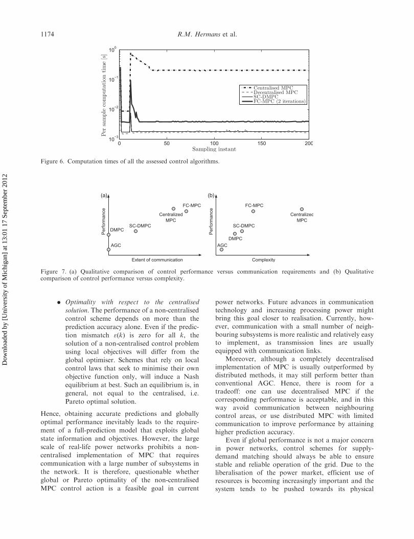
required for computing the optimal input sequence ofcontroller i. These values, obtained for a simulation on a3.48 GB RAM, 2.66 GHz Pentium-E PC, are shown inFigure 6.

The results show that DMPC and SC-DMPC arepreferred from a computational point of view, becausethese techniques require significantly less computa-tional effort compared to centralised MPC. Thecomputational burdens of DMPC and SC-DMPC arecomparable, as their optimisation problems are almostequally sized, except for the additional contractionconstraints in SC-DMPC. The FC-MPC algorithmrequires about twice as much computational time thanSC-DMPC and DMPC if the maximum number ofiterations is set to 2, because the local QPs that FC-MPC solves per iteration have dimensions that arecomparable with those of the SC-DMPC and DMPCoptimisation problems. Thus, although in this simula-tion, the FC-MPC controller needs less computationaleffort than centralised MPC to compute a controlaction, from a complexity point of view, FC-MPC isonly advantageous as long as its number of iterationsis small.

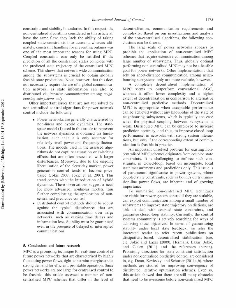
The simulation results are summarised in Figure 7,which indicates that performance is positively

correlated with the extent of communication and thecomplexity of the prediction models/optimisationproblems that underlie the control scheme.

4.3 Assessment

The results obtained in Section 3 and 4.2 indicate thatthere are two important aspects that determine theperformance of a non-centralised MPC technique:

. Prediction accuracy with respect to the centra-lised model. A model that ignores the dynamiccoupling between subsystems introduces aprediction error, i.e. a mismatch between thepredicted (local) state trajectories and the statetrajectories that would result from applyingthe ensemble of local inputs to the fullnetwork of interconnected systems. That is,the prediction error at time k2Zþ of theprediction horizon is given by

"ðkÞ ¼ Ak �xð0Þ þXk�1�¼0

Ak�1��B

�u1ð�Þ

..

.

�uMð�Þ

2664

3775�

�x1ðkÞ

..

.

�xMðkÞ

2664

3775:

ð27Þ

Figure 4. Simulation results of the centralised MPC control and classical AGC control schemes.


Dow

nloa

ded

by [

Uni

vers

ity o

f M

ichi

gan]

at 1

3:01

17

Sept

embe

r 20

12

MPC controllers can exchange their local statepredictions to use them as a measure for thedynamic coupling, and exploit this for increas-ing the prediction accuracy. Accurate predic-tions are important, as solving a controlproblem that is based on inexact predictionsresults in non-optimal closed-loop perfor-mance. Precise predictions are required alsofor state constraint handling, as a constrainedoptimal control action associated with inaccu-rate local predictions can be non-feasible forthe actual coupled system.

Figure 5. Simulation results of the non-centralised MPC control techniques.

Table 1. Performance in terms of settling time and cost.

Settling time (s)

Cost!1 !2 !3 !4 P12tie P23

tie P34tie

AGC 164 165 175 175 235 353 187 530.62MPC 58 48 45 43 56 55 66 176.59FC-MPC (2 iterations) 50 48 45 44 56 55 65 182.44DMPC 64 63 65 72 72 98 79 270.73SC-DMPC 88 114 105 105 138 158 50 260.13

Table 2. Dimensions of the local quadratic programs.

Technique

Size of A (nv� nc)

Example General case

Centralised MPC 400� 200 2NP

i mi�NP

i mi

FC-MPC 100� 50 2N mi�N mi

SC-DMPC 108� 50 2(N miþ ni)�N mi

DMPC 100� 50 2N mi�N mi


Dow

nloa

ded

by [

Uni

vers

ity o

f M

ichi

gan]

at 1

3:01

17

Sept

embe

r 20

12

. Optimality with respect to the centralised

solution. The performance of a non-centralised

control scheme depends on more than the

prediction accuracy alone. Even if the predic-

tion mismatch "(k) is zero for all k, the

solution of a non-centralised control problem

using local objectives will differ from the

global optimiser. Schemes that rely on local

control laws that seek to minimise their own

objective function only, will induce a Nash

equilibrium at best. Such an equilibrium is, in

general, not equal to the centralised, i.e.

Pareto optimal solution.

Hence, obtaining accurate predictions and globally

optimal performance inevitably leads to the require-

ment of a full-prediction model that exploits global

state information and objectives. However, the large

scale of real-life power networks prohibits a non-

centralised implementation of MPC that requires

communication with a large number of subsystems in

the network. It is therefore, questionable whether

global or Pareto optimality of the non-centralised

MPC control action is a feasible goal in current

power networks. Future advances in communicationtechnology and increasing processing power mightbring this goal closer to realisation. Currently, how-ever, communication with a small number of neigh-bouring subsystems is more realistic and relatively easyto implement, as transmission lines are usuallyequipped with communication links.

Moreover, although a completely decentralisedimplementation of MPC is usually outperformed bydistributed methods, it may still perform better thanconventional AGC. Hence, there is room for atradeoff: one can use decentralised MPC if thecorresponding performance is acceptable, and in thisway avoid communication between neighbouringcontrol areas, or use distributed MPC with limitedcommunication to improve performance by attaininghigher prediction accuracy.

Even if global performance is not a major concernin power networks, control schemes for supply-demand matching should always be able to ensurestable and reliable operation of the grid. Due to theliberalisation of the power market, efficient use ofresources is becoming increasingly important and thesystem tends to be pushed towards its physical

Figure 6. Computation times of all the assessed control algorithms.

(a) (b)

Figure 7. (a) Qualitative comparison of control performance versus communication requirements and (b) Qualitativecomparison of control performance versus complexity.


Dow

nloa

ded

by [

Uni

vers

ity o

f M

ichi

gan]

at 1

3:01

17

Sept

embe

r 20

12

constraints and stability boundaries. In this respect, thenon-centralised algorithms considered in this article allhave the same flaw: they lack the ability of takingcoupled state constraints into account, whereas ulti-mately, constraint handling for preventing outages wasone of the most important reasons for using MPC.Coupled constraints can only be satisfied if theprediction of all the constrained states coincides withthe predicted state trajectory of the centralised MPCscheme. This shows that network-wide communicationamong the subsystems is crucial to obtain globallyfeasible state predictions. Note, however, that this doesnot necessarily require the use of a global communica-tion network, as state information can also bedistributed via iterative communication among neigh-bouring subsystems only.

Other important issues that are not yet solved bynon-centralised control algorithms for power networkcontrol include the following:

. Power networks are generally characterised bynon-linear and hybrid dynamics. The state-space model (1) used in this article to representthe network dynamics is obtained via linear-isation, such that it is only accurate forrelatively small power and frequency fluctua-tions. The models used in the assessed algo-rithms do not capture saturation or switchingeffects that are often associated with largerdisturbances. Moreover, due to the ongoingliberalisation of the electricity market, powergeneration control tends to become price-based (Jokic 2007; Jokic et al. 2007). Thistrend comes with the introduction of hybriddynamics. These observations suggest a needfor more advanced, nonlinear models, thusfurther complicating the application of non-centralised predictive control.

. Distributed control methods should be robustagainst the typical disturbances that areassociated with communication over largenetworks, such as varying time delays andinformation loss. Stability must be guaranteedeven in the presence of delayed or interruptedcommunications.

5. Conclusions and future research

MPC is a promising technique for real-time control offuture power networks that are characterised by highlyfluctuating power flows, tight-constraint margins and astrong demand for efficient, profitable operation. Sincepower networks are too large for centralised control tobe feasible, this article assessed a number of non-centralised MPC schemes that differ in the level of

decentralisation, communication requirements andcomplexity. Based on our investigations and analysisof the non-centralised algorithms, the following con-clusions can be drawn.

The large scale of power networks appears toprohibit the application of non-centralised MPCschemes that require extensive communication amonglarge number of subsystems. Thus, globally optimalperforming non-centralised MPC may not be a feasiblegoal for power networks. Other implementations thatrely on short-distance communication among neigh-bouring subsystems only are more realistic, however.

A completely decentralised implementation ofMPC seems to outperform conventional AGC,whereas it offers lower complexity and a higherextent of decentralisation in comparison to alternativenon-centralised predictive methods. DecentralisedMPC is appropriate when acceptable performancecan be achieved without any knowledge of the state ofneighbouring subsystems, which is typically the casewhen the physical coupling between subsystems isweak. Distributed MPC can be employed to increaseprediction accuracy, and thus, to improve closed-loopperformance, in networks with strong system interac-tions, but only if the corresponding extent of commu-nication is feasible in practice.

An important unsolved problem for existing non-centralised MPC schemes originates from coupled stateconstraints. It is challenging to enforce such con-straints, in closed-loop, based on incomplete, localstate measurements and predictions only. This issue isof paramount significance to power systems, wherecoupled state constraints, such as bounds on transmis-sion-line power flows, are inherent and of growingimportance.

To summarise, non-centralised MPC techniquesare viable for power system control if they are scalable,can exploit communication among a small number ofsubsystems to improve state trajectory predictions, areable to deal with coupled state constraints, andguarantee closed-loop stability. Currently, the controlsystems community is actively searching for ways ofachieving these objectives. In terms of guaranteeingstability under local state feedback, we refer theinterested reader to refer recent publications ondissipativity-based, decentralised stabilisation (see,e.g. Jokic and Lazar (2009), Hermans, Lazar, Jokic,and Gielen (2011) and the references therein).Promising directions for state-constraint satisfactionunder non-centralised predictive control are consideredin, e.g. Doan, Keviczky, and Schutter (2011a,b), wheremethods are studied for improving convergence ofdistributed, iterative optimisation schemes. Even so,this article showed that there are still many obstaclesthat need to be overcome before non-centralised MPC


Dow

nloa

ded

by [

Uni

vers

ity o

f M

ichi

gan]

at 1

3:01

17

Sept

embe

r 20

12

can be successfully applied for frequency control inpractice.

Acknowledgements

The authors would like to thank Armand Damoiseaux for hiscontributions to the case studies performed in this article.This work was supported by the EOS-LT Regelduurzaamproject, funded by Agentschap NL, an agency of theDutch Ministry of Economic Affairs, and the EuropeanCommission Research Project FP7-ICT-249096 (E-Price).

Note

1. With ‘settling time’, we mean the time required for astate transient to settle within an error band of 5.10�4

around the steady-state value.

Referencs

Alessio, A., and Bemporad, A. (2007), ‘Decentralised Model

Predictive Control of Constrained Linear Systems’,in Proceedings European Control Conference, Kos,

Greece, pp. 2813–2818.Bemporad, A., Morari, M., Dua, V., and Pistikopoulos, E.N.

(2002), ‘The Explicit Linear Quadratic Regulator forConstrained Systems’, Automatica, 38, 2–30.

Blanchini, F. (1994), ‘Ultimate Boundedness Control forUncertain Discrete-time Systems via Set-induced

Lyapunov Functions’, IEEE Transactions on AutomaticControl, 39, 428–433.

Borbely, A.-M., and Kreider, J.F. (2001), DistributedGeneration: the Power Paradigm for the New Millennium,

Boca Raton, FL, USA: CRC Press.Camponogara, E., (2000), ‘Controlling Networks withCollaborative Nets’, PhD Thesis, Carnegie Mellon

University, Pittsburgh, Pennsylvania.Camponogara, E., Jia, D., Krogh, B.H., and Talukdar, S.

(2002), ‘Distributed Model Predictive Control’, IEEEControl Systems Magazine, 22, 44–52.

Doan, M.D., Keviczky, T., and Schutter, B.D. (2011a), ‘ADistributed Optimisation-based Approach for Hierarchical

MPC of Large-scale Systems with Coupled Dynamics andConstraints’, in Conference on Decision and Control,

Orlando, FL, USA.Doan, M.D., Keviczky, T., and Schutter, B.D. (2011b), ‘An

Iterative Scheme for Distributed Model Predictive Controlusing Fenchel’s Duality’, Journal of Process Control, 21,

746–755.Dunbar, W.B. (2007), ‘Distributed Receding

Horizon Control of Dynamically Coupled NonlinearSystems’, IEEE Transactions on Automatic Control, 52,

1249–1263.

Goodwin, G.C., Seron, M.M., and De Dona, J.A. (2005),‘Constrained Control and Estimation: an Optimisation

Approach’, Communications and Control Engineering,London, UK: Springer.

Hermans, R.M., Lazar, M., Jokic, A., and Gielen, R.H.(2011), ‘On Parameterised Stabilisation of Networked

Dynamical Systems’, in 18th IFAC World Congress,Milano, Italy.

Jaleeli, N., VanSlyck, L., Ewart, D., Fink, L., and

Hoffmann, A. (1992), ‘Understanding AutomaticGeneration Control’, IEEE Transactions on PowerSystems, 7, 1106–1122.

Jokic, A. (2007), ‘Price-based Optimal Control of ElectricalPower Systems’, PhD Thesis, Eindhoven University ofTechnology, The Netherlands.

Jokic, A., and Lazar, M. (2009), ‘On Decentralised

Stabilisation of Discrete-time Nonlinear Systems’,in American Control Conference, St. Louis, MI,pp. 5777–5782.

Jokic, A., Lazar, M., and Van den Bosch, P.P.J. (2007),‘Price-based Optimal Control of Power Flow in ElectricalEnergy Transmission Networks’, in Hybrid Systems:

Computation and Control, Lecture Notes in ComputerScience (Vol. 4416), Pisa, Italy: Springer Verlag,pp. 315–328.

Keviczky, T., Borrelli, F., and Balas, G.J. (2006),‘Decentralised Receding Horizon Control for Large ScaleDynamically Decoupled Systems’, Automatica, 42,2105–2115.

Kundur, P. (1994), Power System Stability and Control,New York, NY, USA: McGraw-Hill.

Mayne, D.Q., Rawlings, J.B., Rao, C.V., and Scokaert,

P.O.M. (2000), ‘Constrained Model Predictive Control:Stability and Optimality’, Automatica, 36, 789–814.

Muske, K.R., and Badgwell, T.A. (2002), ‘Disturbance

Modelling for Offset-free Linear Model PredictiveControl’, Journal of Process Control, 12, 617–632.

Pannocchia, G., and Rawlings, J.B. (2003), ‘Disturbance

Models for Offset-free Model-predictive Control’, AIChEJournal, 49, 426–437.

Richards, A., and How, J.P. (2007), ‘Robust DistributedModel Predictive Control’, International Journal of

Control, 80, 1517–1531.Stoft, S. (2002), Power System Economics: Designing Marketsfor Electricity, Piscataway, NJ, USA: IEEE Press/Wiley-

Interscience.Venkat, A.N. (2006), ‘Distributed Model Predictive Control:Theory and Applications’, PhD Thesis, University of

Wisconsin-Madison, Madison, WI, USA.Venkat, A.N., Hiskens, I.A., Rawlings, J.B., and Wright, S.J.(2008), ‘Distributed MPC Strategies with Application toPower System Automatic Generation Control’, IEEE

Transactions on Control Systems Technology, 16,1192–1206.


Dow

nloa

ded

by [

Uni

vers

ity o

f M

ichi

gan]

at 1

3:01

17

Sept

embe

r 20

12

Appendix: List of parameter values

Table A1 lists the parameter values used in our simulation.

Table A1. Simulation parameters.

Sampling period 1 sSimulation time 200 sPrediction horizon N 50Iterations (FC-MPC) 2State of subsystem 1 x1¼ col(DPV1, DPM1, D!1)State of subsystem 2 x2¼ col(D�12, DPV2, DPM2, D!2)State of subsystem 3 x3¼ col(D�23, DPV3, DPM3, D!3)State of subsystem 4 x4¼ col(D�34, DPV4, DPM4, D!4)Disturbance DPL1

0, 8tDisturbance DPL2

0 for t5 10, þ0.25 for t� 10Disturbance DPL3

0 for t5 10, �0.25 for t� 10Disturbance DPL4

0, 8tConstraint on �0:5 � DPrefi � 0:5DPrefi , i ¼ 1, . . . , 4Generator damping: 3, 0.275, 2, 2.75D1, D2, D3, D4

Generator inertia: 4, 40, 35, 10J1, J2, J3, J4Speed regulation: 0.12, 0.28, 0.16, 0.12r1, r2, r3, r4Governor time constant: 4, 25, 15, 5�G1, �G2, �G3, �G4Turbine time constant: 5, 10, 20, 10�T1, �T2, �T3, �T4Tie-line gain: 2.54, 1.5, 2.5b12, b23, b34AGC gain 1: 0.01, 0.02, 0.03, 0.01K1, K2, K3, K4

AGC gain 2: 36.33, 14.56, 27.00, 36.08B1, B2, B3, B4

Q1, Q2 100 � diag(0, 0, 5), 100 � diag(5, 0, 0, 5)Q3, Q4 100 � diag(5, 0, 0, 5), 100 � diag(5, 0, 0, 5)R1, R2, R3, R4 1, 1, 1, 1


Dow

nloa

ded

by [

Uni

vers

ity o

f M

ichi

gan]

at 1

3:01

17

Sept

embe

r 20

12

international journal of control - university of...

Documents