intermittent state-space model for demand · pdf fileintermittent state-space model for ......

LC F

Introduction Universal model Constant p Croston TSB Experiment Finale References

Intermittent state-space model for demandforecasting

Ivan Svetunkov and John Boylan

19th IIF Workshop

29th June 2016

Lancaster Centre for

Forecasting

Ivan Svetunkov and John Boylan LCF

Intermittent state-space model for demand forecasting

LC F


Motivation

Croston (1972) proposes a method for intermittent demandforecasting, mentioning the model: yι = xt · zt

He estimates probability using intervals between demands ( 1qt

).

He also assumes that probability is constant between occurrences.

Syntetos and Boylan (2001, 2005) show that the conditionalexpectation of Croston’s method is biased.

They propose an approximation, that corrects the error.



LC F


Motivation

Snyder (2002) looks at Croston’s method in details, claiming thatthe underlying model is: yι = xt · zt + εt.

This model produces both positive and negative data.

This is a drawback, so Snyder (2002) proposes a modification,taking exp of non-zero demands.



LC F


Motivation

Shenstone and Hyndman (2005) study several additive models,possibly underlying Croston’s method.

They argue that any model underlying Croston’s method must be:

• non-stationary,

• defined on continuous space.

They conclude that the implied model has non-realistic properties.

They support Snyder (2002) approach with exp.



LC F


Motivation

Teunter et al. (2011) propose a model taking inventoryobsolescence into account.

The probability of having a demand is decreasing when demanddoes not occur.

Simulation is done, but estimation of parameters is skipped.

In the following paper Zied Babai et al. (2014) optimise severalmethods, including TSB.

They use MSE calculated as a difference between the estimate andthe actual demand.



LC F


Motivation

Kourentzes (2014) investigates the estimation of Croston, SBA,TSB.

He discusses several cost functions.

And proposes two new ones, which improves estimation ofmethods.

He finds that optimisation of initial states increases forecastingaccuracy.



LC F


Motivation, overall

There is no concise model, underlying all the methods.

Because of Shenstone and Hyndman (2005) we believe that itdoesn’t exist.

Intermittent demand methods are disconnected from slow-movingdata methods.

And we still need to make good decisions about replenishmentlevels.



Universal model

LC F


Universal model

Very general model:yt = otyt, (1)

where ot ∼ Bernoulli(pt) and yt is a statistical model of our choice.

This corresponds to Croston’s original idea.

If ot = 1, for any t, then this is slow-moving data model.



LC F


Additive state-space model (Snyder, 1985)

State-space model:

yt = ot(w′vt−1 + εt)

vt = Fvt−1 + gεt, (2)

vt−1 vector of states, w is measurement vector,F is transition matrix, g is persistence vector,εt ∼ N(0, σ2).

Example. iETS(A,N,N) with constant probability:

yt = ot(lt−1 + εt)lt = lt−1 + αεt

, (3)

where ot ∼ Bernoulli(p).



LC F


General state-space (based on Hyndman et al. (2008))

State-space model for any ETS:

yt = ot (w(vt−1) + r(vt−1, εt))vt = F (vt−1) + g(vt−1, εt)

. (4)

Example. iETS(M,Ad,N) with constant probability:

yt = ot(lt−1 + φbt−1)(1 + εt)lt = (lt−1 + φbt−1)(1 + αεt)bt = φbt−1(1 + βεt)

, (5)

where ot ∼ Bernoulli(p), (1 + εt) ∼ logN(0, σ2).



LC F


Advantages

What are the advantages of such a model?

• Statistical rationale for intermittent demand;

• Connection between conventional and intermittent models;

• Correct estimation of mean;

• Simpler variance estimation;

• Prediction intervals;



LC F


Advantages

What else?

• Both additive and multiplicative ETS models;

• Any statistical model;

• Likelihood function;

• Solution to initialisation and optimisation problems;

• Model selection.



LC F


Disadvantages

What are the disadvantages of such a model?

• May need more observations...

• ...Especially for trend and seasonal models;

• Derivations in some cases may be messy.



iETS(M,N,N),

constant probability

LC F


iETS(M,N,N), constant probability

iETS(M,N,N) model has the form:

yt = otlt−1(1 + εt)lt = lt−1(1 + αεt)

, (6)

where ot ∼ Bernoulli(p).

iETS(M,N,N) underlies SES (Hyndman et al., 2008).

Conditional expectation:

E(yt+h|t) = pE(yt+h|t) = pw′F h−1vt = plt.



LC F



Conditional variance:

V (yt+h|t) = p(1− p)l2t + pl2t σ2

1 + α2(1 + σ2)

h−1∑j=1

(1 + α2σ2)

.

Messy because of the multiplicative error.



LC F



Likelihood can be derived taking probabilities:

P (yt|ot = 1, θ, σ2) = p 1yt

1√2πσ2

e−(1+εt)

2

2σ2 ,

P (yt|ot = 0, θ, σ2) = 1− p.

Product of all the zero and non-zero cases is then:

L(θ, σ2|yt) =∏ot=1

p1

yt

1√2πσ2

e−(1+εt)

2

2σ2

∏ot=0

(1− p). (7)



LC F



The concentrated log-likelihood is simple:

`(θ, σ2|yt) = −T12

(log (2πe) + log

(σ2))−∑ot=1

log(yt)

+T0 log(1− p) + T1 log p,(8)

where T is number of all observations, T0 is number of zeroes, T1number of non-zero demands.

The variance of the error estimated using likelihood (8) is:

σ2 =1

T1

∑ot=1

(1 + εt).

The probability can also be derived from (8): p = T1T .



LC F


Example. Intermittent demand

0 50 100 150 200 250

05

1015

20

ETS(MNN)

SeriesFitted values

Point forecast95% prediction interval

Forecast origin



LC F


Example. Probabilities

0 50 100 150 200 250

0.0

0.2

0.4

0.6

0.8

1.0

Constant probability

SeriesFitted values

Point forecastForecast origin



LC F


Simple iETS. Sub-conclusion

• Pretty easy statistical model;

• Multiplicative ETS is possible and makes more sense thanadditive;

• But probability is currently constant;



iETS(M,N,N),

time varying probability,

Croston style

LC F


Croston’s iETS(M,N,N)

ETS(M,N,N) + compound Bernoulli distribution:ot ∼ Bernoulli(pt), where pt =

11+qt

,qt are intervals between demands. If qt = 0, then pt = 1.

Assumption: Probability changes only when demand occurs.

State-space model for probabilities:

qt = lq,t−1(1 + εt)lq,t = lq,t−1(1 + δεt)

, (9)

where (1 + εt) ∼ logN(0, σ2q )



LC F



Overall iETS(M,N,N) Croston style is:


qt = lq,t−1(1 + εt)lq,t = lq,t−1(1 + δεt)

(1 + εt) ∼ logN(0, σ2)ot ∼ Bernoulli( 1

1+qt)

(1 + εt) ∼ logN(0, σ2q ).

(10)

Now it becomes a bit more complicated...



LC F



Conditional expectation:

E(yt+h|t) = ltE

(1

1 + qt+h

∣∣∣∣ t) .Not yet simplified:

E(yt+h|t) = ltE

(1

1 + lq,t∏h−1j=1 (1 + δεt+j)(1 + εt+h)

∣∣∣∣∣ t).

We feel that this should be close to SBA.



LC F



Variance is currently mind blowing...

But it should be based on the variance of ot:σ2o = pt(1− pt)

Meaning that the conditional variance of yt+h is:

V (yt+h|t) = E(

11+qt+h

∣∣∣ t)(1− E ( 11+qt+h

∣∣∣ t)) l2t+E

(1

1+qt+h

∣∣∣ t) l2t σ2 (1 + α2(1 + σ2)∑h−1

j=1 (1 + α2σ2)).



LC F



Likelihood however can be done in two stages(assuming demand sizes and intervals are independent):

1. Likelihood for intervals;

2. Likelihood for demands.

Both of them are based on lognormal distributions.



LC F



Concentrated log-likelihoods.For intervals (first stage):

`(θq, σ2q |qt) = −

Tq2

(log (2πe) + log

(σ2q))−

Tq∑t=1

log(qt), (11)

For demands (second stage):

`(θ, σ2|yt) = −T12

(log (2πe) + log

(σ2))−∑ot=1

log(yt)

+∑ot=0

log(1− pt) +∑ot=1

log pt,(12)



LC F


Croston’s iETS(M,N,N). Example

0 50 100 150 200 250

05

1015

20

ETS(MNN)

SeriesFitted values


Forecast origin



LC F


Croston’s iETS(M,N,N). Example. Probabilities

0 50 100 150 200 250

0.0

0.2

0.4

0.6

0.8

1.0

Croston probability

SeriesFitted values




LC F


Croston’s iETS. Sub-conclusion

• There is a statistical model underlying Croston’s method;

• Conditional expectation should be closer to SBA;

• Conditional variance can be found analytically;

• Probabilities are updated only when demand occurs;

• There are still some problems with derivations.



iETS(M,N,N),

time varying probability,

TSB

LC F


TSB iETS(M,N,N)

ETS(M,N,N) + compound Bernoulli distribution:ot ∼ Bernoulli(pt), where:

pt = lp,t−1(1 + ξt)lp,t = lp,t−1(1 + δξt)

. (13)

pt can be estimated as naıve probability: pt = ot.

We want to have conditional Beta(a, b) distribution.

But this means that pt ∈ (0, 1).

We need boundary values!



LC F


TSB iETS(M,N,N)

Temporary fix – simple transfer function:

p′t = (1− 2κ)pt + κ,

where κ is some small number. e.g. κ = 10−20.

This means that p′t ∈ (κ, 1− κ).

So p′t ∼ Beta(a,b).



LC F


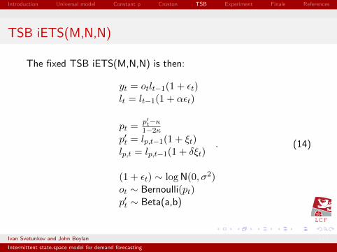
TSB iETS(M,N,N)

The fixed TSB iETS(M,N,N) is then:


pt =p′t−κ1−2κ

p′t = lp,t−1(1 + ξt)lp,t = lp,t−1(1 + δξt)

(1 + εt) ∼ logN(0, σ2)ot ∼ Bernoulli(pt)p′t ∼ Beta(a,b)

. (14)



LC F


TSB iETS(M,N,N)

Conditional expectation is simpler than in Croston:

E(yt+h|t) = ltlp,t−1 − κ1− 2κ

.

Conditional variance is based on Bernoulli pt+h|t(1− pt+h|t):

V (yt+h|t) = lp,t−1−κ1−2κ

(1− lp,t−1−κ

1−2κ

)l2t

+lp,t−1−κ1−2κ l2t σ

2

1 + α2(1 + σ2)

h−1∑j=1

(1 + α2σ2)

.



LC F


TSB iETS(M,N,N)

Concentrated log-likelihood in two stages.For the probability (stage 1):

`(θp, a, b|pt) = (a− 1)

T∑t=1

log(lp,t−1(1 + ξt))

+(b− 1)

T∑t=1

log(1− lp,t−1(1 + ξt))

−T logB(a, b),

(15)

For the demand sizes (stage 2):

`(θ, σ2|yt) = −T12

(log (2πe) + log

(σ2))−∑ot=1

log(yt)

+∑ot=0

log(1− pt) +∑ot=1

log pt,(16)



LC F


TSB iETS(M,N,N). Example

0 50 100 150 200 250

05

1015

20

ETS(MNN)

SeriesFitted values


Forecast origin



LC F


TSB iETS(M,N,N). Example. Probabilities

0 50 100 150 200 250

0.0

0.2

0.4

0.6

0.8

1.0

TSB probability

SeriesFitted values




LC F


TSB iETS. Sub-conclusion

• There is a statistical model underlying TSB;

• Estimation problem solved;

• Works fine even with the proposed approximation;

• pt is unknown, problem with estimation;

• Problem with distribution of pt;

• Multiplicative damped trend could be more appropriate.



Real time series example

LC F


Example on the real data

1. 58 intermittent time series,

2. One product, different branches, daily data,

3. 248 observations each, 10 – 103 demand occurrences,

4. Holdout sample of 20 obs,

5. iETS using ”es” from ”smooth” package in R(https://github.com/config-i1/smooth):

I Stable probability,I Croston’s probability,I TSB probability,

6. Croston’s method and TSB, ”tsintermittent” package in R.



https://github.com/config-i1/smooth

LC F


Example on the real data

Method sPIS sAPIS ARMSE Complex bias

iETS, stable -609.2 2219.6 1.00 -46.3%iETS, Croston -442.0 2299.4 0.99 -48.4%iETS, TSB -538.2 2082.3 0.92 -46.1%Croston’s method -256.0 2158.9 1.03 -53.2%TSB method -279.6 2116.2 1.03 -52.8%Zero forecast -2363.6 2363.6 0.82 99.5%

Table: Intermittent demand data performance.



Conclusions

LC F


Conclusions

• We proposed a very simple modification, that can be appliedto any model;

• iETS is one of such models;

• Multiplicative models are available now;

• Model selection is also available;

• It can even be done between Stable / Croston / TSB;



LC F


Conclusions

• Conditional expectation can be correctly estimated;

• The same holds for the conditional variance;

• Prediction intervals for intermittent data;

• Croston and TSB have underlying iETS model;

• Estimation problem is now solved for them.



Finale

Thank you for your attention!

Ivan Svetunkov, John Boylan

[email protected]@lancaster.ac.uk

Lancaster Centre for

Forecasting

mailto:[email protected]

mailto:[email protected]

LC F


Croston, J. D., 1972. Forecasting and Stock Control forIntermittent Demands. Operational Research Quarterly(1970-1977) 23 (3), 289.

Hyndman, R. J., Koehler, A., Ord, K., Snyder, R., 2008.Forecasting with Exponential Smoothing. Springer BerlinHeidelberg.

Kourentzes, N., 2014. On intermittent demand model optimisationand selection. International Journal of Production Economics156, 180–190.

Shenstone, L., Hyndman, R. J., 2005. Stochastic modelsunderlying Croston’s method for intermittent demandforecasting. Journal of Forecasting 24 (6), 389–402.

Snyder, R., 2002. Forecasting sales of slow and fast movinginventories. European Journal of Operational Research 140 (3),684–699.

Snyder, R. D., 1985. Recursive Estimation of Dynamic LinearIvan Svetunkov and John Boylan LCF


LC F


Models. Journal of the Royal Statistical Society, Series B(Methodological) 47 (2), 272–276.

Syntetos, A., Boylan, J., 2001. On the bias of intermittent demandestimates. International Journal of Production Economics71 (1-3), 457–466.

Syntetos, A. A., Boylan, J. E., 2005. The accuracy of intermittentdemand estimates. International Journal of Forecasting 21 (2),303–314.

Teunter, R. H., Syntetos, A. A., Zied Babai, M., 2011. Intermittentdemand: Linking forecasting to inventory obsolescence.European Journal of Operational Research 214 (3), 606–615.

Zied Babai, M., Syntetos, A., Teunter, R., 2014. Intermittentdemand forecasting: An empirical study on accuracy and therisk of obsolescence. International Journal of ProductionEconomics 157 (1), 212–219.



intermittent state-space model for demand · pdf fileintermittent state-space model for ......

Documents