interior point method for long-term generation scheduling
TRANSCRIPT

Ann Oper ResDOI 10.1007/s10479-008-0389-z
Interior point method for long-term generationscheduling of large-scale hydrothermal systems
Anibal Tavares Azevedo ·Aurelio Ribeiro Leite Oliveira · Secundino Soares
© Springer Science+Business Media, LLC 2008
Abstract This paper presents an interior point method for the long-term generation schedul-ing of large-scale hydrothermal systems. The problem is formulated as a nonlinear program-ming one due to the nonlinear representation of hydropower production and thermal fuel costfunctions. Sparsity exploitation techniques and an heuristic procedure for computing the in-terior point method search directions have been developed. Numerical tests in case studieswith systems of different dimensions and inflow scenarios have been carried out in order toevaluate the proposed method. Three systems were tested, with the largest being the Brazil-ian hydropower system with 74 hydro plants distributed in several cascades. Results showthat the proposed method is an efficient and robust tool for solving the long-term generationscheduling problem.
Keywords Hydrothermal generation scheduling · Long-term operational planning ·Nonlinear optimization · Interior point method
This research was supported in part by the Foundation for the Support of Research of the Stateof São Paulo (FAPESP), by the Brazilian Council for the Development of Science and Technology(CNPq), and by the Superior Level Coordination for Personal Development (CAPES), Brazil.
A.T. Azevedo (�)Av. Ariberto Pereira da Cunha, 333, Mathematic Department, Paulista State University, Guaratinguetá,SP, 12516-410, Brazile-mail: [email protected]
A.R.L. OliveiraRua Sergio Buarque de Holanda, 651, Applied Mathematic Department, State University of Campinas,Campinas, SP, 13083-970, Brazile-mail: [email protected]
S. SoaresRua Albert Einstein, 400, School of Electrical and Computer Engineering, State Universityof Campinas, Campinas, SP, 13083-852, Brazile-mail: [email protected]

Ann Oper Res
1 Introduction
The operational planning of hydrothermal power systems is designed to provide a reliableand economic operational policy that embraces time frames ranging from the long-termmanagement of hydropower resources to the electric and hydraulic aspects of daily genera-tion dispatch.
Due to the large scale and complexity of this problem, it has usually been approached bydecomposition into two hierarchically connected problems, long-term generation scheduling(LTGS) and short-term generation scheduling (STGS).
LTGS covers a planning period of one or more years, divided into monthly intervals,with the first month being divided into weeks. The objective of this planning is to controlthe water storage in the reservoirs in order to maximize hydroelectric production and, as aresult, minimize the cost of non-hydraulic generation sources. LTGS planning provides aweekly generation target for each hydro plant.
STGS covers the next week ahead, usually divided into hourly intervals. Its goal is toobtain a generation scheduling that matches the long-term generation targets for each hydroplant and optimizes the efficiency of hydropower conversion. This planning should comprisea detailed representation of hydro plant operational characteristics and the security operationof the electrical transmission system (Soares and Salmazo 1997).
The present paper deals with the modeling and resolution of the LTGS problem. This,by itself, is very difficult due to aspects such as the long-term horizon to be analyzed, thestochastic nature of water inflows, the operational interconnection between hydro plants inthe same cascade, and the nonlinear nature of the functions of hydropower production andnon-hydraulic generation cost.
To cope with the stochastic nature of the LTGS problem, one common approach is toconsider the randomness of inflows by their probability distribution functions and applyclassical optimization techniques based on stochastic dynamic programming (SDP). Thisapproach requires some sort of simplification, however, due to the well known “curse ofdimensionality” associated with SDP problems (Bellman 1962). This simplification can bein the representation of the multireservoir system using aggregated composite models (Ar-avanitidis and Rosing 1970; Saad et al. 1996; Turgeon 1980; Valdes et al. 1995) or in thesolution procedure, such as the use of Bender’s decomposition (Pereira and Pinto 1991),which linearizes the problem (Ponnambalam 2002).
Another common approach is based on the solution of a deterministic model within theframework of a scenario technique (Dembo 1991; Escudero et al. 1996; Nabona 1993). Inthis approach, the solution of the stochastic problem is obtained from the solutions of thedeterministic model for a set of different scenarios representing the stochastic nature ofinflows. The advantage of the scenario approach to the LTGS problem is that it does notrequire simplification for the handling of multireservoir systems, which is quite importantwhen large-scale hydrothermal power systems are involved.
Thus, in the framework of a scenario technique for LTGS problems, a robust and efficienttool is crucial for solving the deterministic version of the problem since it must be appliedseveral times for different inflow scenarios. Moreover, for the purpose of simulation, thedecision process has to be repeated for each time interval in order to update the storage inthe reservoirs in an open-loop feedback control framework (Martinez and Soares 2002).
Several techniques have been suggested for the solution of this problem, including non-linear programming (Gagnon et al. 1974; Hanscom et al. 1980) and network flow ap-proaches (Carvalho and Soares 1987; Lyra and Tavares 1988; Oliveira and Soares 1995;Rosenthal 1981; Sjvelgren et al. 1983). More recently, the option of using interior point

Ann Oper Res
methods (IPMs) which are especially efficient for solving large scale optimization prob-lems, has arise.
The first IPM was developed by Dikin (1967). A later IPM for solving Linear Program-ming (LP) problems was developed by Karmarkar (1984), and results of its use presented byAdler et al. (1989). Since then, IPMs have undergone extensive development and are nowbeing applied for the solution of many optimization problems. Mehrotra (1992) has pro-posed a predictor-corrector method for obtaining the search directions of an interior pointprimal-dual method which has proved to be the most efficient of the IPMs for LP.
More recently, IPM-based techniques have been applied in a variety of power systemsproblems, such as optimal active power dispatch (Oliveira et al. 2003), optimal reactivedispatch (Granville 1994; Torres and Quintana 1998), and security-constrained economicdispatch (Yan and Quintana 1997). A comprehensive survey of the application of IPM topower systems is provided by Quintana et al. (2000).
Research on IPMs for the linearized version of LTGS problem has also been publishedas reported in (Christoforidis et al. 1996; Ponnambalam et al. 1992; Medina et al. 1999).Ponnambalam et al. (1992) implemented a dual affine algorithm to solve a linear version ofthe LTGS problem, and Christoforidis et al. (1996) suggested a commercial code assuming apiecewise linear hydro production function. Medina et al. (1999) solved the problem by alsoassuming linear objective function and constraints. These IPMs have all solved the LTGSproblem by simplifying the nonlinear nature of the problem in some way.
The present paper is concerned with the development of an efficient IPM for solvingthe deterministic version of the LTGS problem for large-scale hydrothermal systems. Theproblem is formulated precisely by considering nonlinear functions for hydroelectric gen-eration and non-hydraulic operational costs. To overcome difficulties related to the preciserepresentation of nonlinear objective function, a specialized IPM capable of exploiting thesparse structure of the problem and handling its Hessian indefiniteness efficiently is nec-essary. Thus, two improvements have been implemented: that of (Gondzio and Sarkissian2003) has been expanded to handle the sparse pattern and nonlinear objective function, whilea new heuristic procedure has been developed to handle Hessian indefiniteness.
The optimality of this IPM has been tested in three different case studies, and its perfor-mance evaluated. The first of these corresponds to a hydrothermal system composed of asingle hydro plant in order to allow a detailed analysis of the optimal solution; the secondcorresponds to a hydrothermal system composed of 15 hydro plants in a single cascade,whereas the third involves the entire Brazilian hydropower system with 74 hydro plants dis-tributed in several cascades. All these case studies considered a five-year planning horizonwhich is that adopted by the Brazilian Independent System Operator (ISO). The results,evaluated on the basis of the number of iterations and the computational time attest to theefficiency of the proposed method.
The outline of the paper is as follows. Notation and modeling of the LTGS problem arepresented in Sects. 2 and 3. The proposed IPM is presented in Sect. 4 and test results aredescribed in Sect. 5. Finally, conclusions are stated in Sect. 6.
2 Notation
t Month index.T Number of months in the planning period.i Hydro plant index.N Number of hydro plants.

Ann Oper Res
Ωi Set of immediate upstream plants for plant i.Ψt Operational cost (dollars).Ht Total hydroelectric generation (MW).hit Hydroelectric generation function (MW).Dt Load demand (MW).rit Water storage in reservoir (m3).rit , rit Bounds on reservoir storage.qit Water discharge through turbines (m3/s).q
it, qit Bounds on water discharge.
vit Water spillage from reservoir (m3/s).ki Constant factor (MW/m3/s/m).φi Forebay elevation function (m).θi Tailrace elevation function (m).ςi(qit ) Penstock head loss function (m).yit Incremental water inflow (m3/s).Δtt Number of seconds in a month.n Double the number of all nonnegative variables.
3 Problem formulation
The LTGS problem can be formulated as the following nonlinear programming problem:
MinT∑
t=1
Ψt
(Dt −
N∑
i=1
hit
)(1)
subject to
(rit − rit−1)/Δtt =∑
j∈Ωi
(qjt + vjt ) − (qit + vit ) + yit (2)
rit ≤ rit ≤ rit (3)
qit
≤ qit ≤ qit (4)
vit ≥ 0 (5)
ri1, ∀i, i = 1,2, . . . ,N, given
∀t, t = 2,3, . . . , T , ∀i, i = 1,2, . . . ,N (6)
where
hit = ki
(φi
(rit + rit−1
2
)− θi(qit + vit ) − ςi(qit )
)qit
The objective function (1) minimizes the operational cost Ψt which represents the mini-mal cost for complementary non-hydraulic sources, such as thermoelectric generation, im-ports from neighboring systems, and load shortage. The operational cost Ψt obtained fromthe optimal economic dispatch of these non-hydraulic sources results in a convex increasingoperational cost function.
The definition of hit represents a precise modeling of hydro generation as a functionof net water head and water discharge through the turbines. The constant ki depends on

Ann Oper Res
water density, gravity acceleration, and average turbine-generator efficiency. Forebay φi(·)and tailrace elevations θi(·) are represented by polynomial functions of storage and releasevariables, respectively, while forebay elevation φi(·) is calculated on the basis of the averagestorage during a month. Tailrace elevation θi(·) depends on discharge and spillage variables.Penstock head loss ςi(·) is a function of water discharge.
The equality constraints in (2) represent the water balance in the reservoir for each month.No time delay for water displacement is being considered in this formulation, since theproblem is concerned with LTGS, which encompasses the time interval of a month.
Lower and upper bounds on variables, expressed by constraints (3)–(5), are imposed bythe physical operational constraints of the hydro plant, as well as other constraints associatedwith multiple uses of water, such as irrigation, navigation, and flood control.
One important feature of model (1)–(6) is the precise representation of hydropower out-put by hit . All nonlinear relations which influence the water head, such as forebay and tail-race elevations, and penstock head loss, were taken into consideration. Therefore, the mainobjective of LTGS, which is the optimal seasonal management of reservoir storage, can bemet precisely, although this may not be assured by models assuming simplified hydropoweroutput functions based on linear and/or piecewise linear approximations such as the IPMsproposed in the literature.
4 Solution technique
4.1 Mathematical formulation
Problem (1)–(6) has the following matricial formulation:
Min f (x)
s.t. Ax = b
x ≤ x ≤ x
(7)
By introducing slack variable vector s and the transformation x = x + x, the system (7)can be transformed into:
Min f (x)
s.t. Ax = b − Ax = b
x + s = x − x = x
x, s ≥ 0
(8)
The primal of the log-barrier problem (8) can now be written (with a “ ˜ ” omitted toprovide a cleaner notation) as
Min f (x) − μ
n∑
i=1
(ln si + lnxi)
s.t. Ax = b
x + s = x
(9)
where μ is a decreasing sequence of positive barrier parameters such that limk→∞ μk = 0.The computation of this value is explained in Sect. 4.6. The Lagrangian function associated

Ann Oper Res
with (7) is:
� ≡ f (x) + yt (b − Ax) + wt(x + s − x) − μ
n∑
i=1
(ln si + lnxi)
The following KKT equations can thus be derived:
Kμ(x, y,w, s) ≡
⎡
⎢⎢⎣
�x
�y
�w
�s
⎤
⎥⎥⎦ =
⎡
⎢⎢⎣
∇f (x) − Aty + w − μX−1e
b − Ax
x + s − x
SWe − μe
⎤
⎥⎥⎦ = 0
where uppercase letters stand for diagonal matrices with entries being the elements of thecorresponding lowercase-letter vectors, and e = (1,1, . . . ,1)t .
Letting Ze = μX−1e and defining v ≡ [x, y,w, z, s]t , the Newton direction is obtainedby solving the following linear system:
K ′μ(v)Δv = −Kμ(v)
⎡
⎢⎢⎢⎢⎣
−H(x) At −I I 0A 0 0 0 0I 0 0 0 I
0 0 S 0 W
Z 0 0 X 0
⎤
⎥⎥⎥⎥⎦
⎡
⎢⎢⎢⎢⎣
Δx
Δy
Δw
Δz
Δs
⎤
⎥⎥⎥⎥⎦=
⎡
⎢⎢⎢⎢⎣
rd
rp
ra
rb
rc
⎤
⎥⎥⎥⎥⎦
(10)
where Kμ(v) = [−�x,�y,�w,�s ,�z]t , �z = XZe − μe, H(x) = ∇2f (x), rd = ∇f (x) −Aty + w − z, rp = Ax − b, ra = x − x − s, rb = μe − SWe and rc = μe − XZe.
To solve the problem, system (10) is reduced by making a number of substitutions, lead-ing to the following normal equation system:
(AD−1At)Δy = rp + AD−1rk (11)
where D = H(x) + S−1W + X−1Z and rk = rd + S−1(rb − Wra) − X−1rc .Matrix H(x) may be indefinite, but it can be transformed to a quasidefinite one, i.e.,
a matrix that is strongly factorizable and to which a Cholesky-like factorization LDLt canbe applied. For this purpose the procedure described by (Altman and Gondzio 1999) and(Benson et al. 2000) is employed. For interior-point methods, the initial point is interior(nonnegative variables are kept strictly positive) and the step is controlled so that the se-quence of points remain interior.
A summary of the necessary calculations for the IPM proposed is provided in Table 1.Some aspects of this IPM, such as the exploitation of sparsity, IPM improvement, initialpoint, step length, computing μ and stopping criteria are discussed and detailed in Sects. 4.2,4.3, 4.4, 4.5, 4.6 and 4.7, respectively.
4.2 Exploiting sparsity
Since the major burden for IPM stems from the solution of normal equations (11), its effi-ciency depends on the exploitation of the sparse pattern of matrices A and D. Let
x = [r q v
]t

Ann Oper Res
Table 1 Primal-Dual IPM forLTGS IPM Direction Computation
Given (x0, s0,w0, z0) > 0, y0 free and τ ∈ (0,1);
For k = 0,1, . . .
μk = σγ k/n,
where: n is twice the number of all nonnegative variables,
γ k is the GAP and γ k/n is the mean GAP.
rkd
= ∇f (xk) − Atyk + wk − zk
rkp = b − Axk
rka = x − xk − sk
rkb
= μke − SkWke
rkc = μke − XkZke
rkk
= rkd
+ S−1(rkb
− Wrka ) − (Xk)−1rk
c
Dk = (H(xk) + (Sk)−1Wk + (Xk)−1Zk)
Δyk = (A(Dk)−1At )−1(rkp + A(Dk)−1rk
k)
Δxk = (Dk)−1(AtΔyk − rkk)
Δsk = rka − Δxk
Δwk = (Sk)−1(rkb
− WkΔsk)
Δzk = (Xk)−1(rkc − ZkΔxk)
αkp = Min
{Min
∂xki<0
(−xki
∂xki
), Min∂sk
i<0
(−ski
∂ski
)}
αkd
= Min
{Min
∂wki<0
(−wki
∂wki
), Min∂zk
i<0
(−zki
∂zki
)}
yk+1 = yk + αkdΔyk
xk+1 = xk + αkpΔxk
sk+1 = sk + αkpΔsk
wk+1 = wk + αkdΔwk
zk+1 = zk + αkdΔzk
k ← k + 1
Until convergence
then matrices A and D have the following structure
A = [A S S
]
and
D =⎡
⎣D1 D4 0D4 D2 D5
0 D5 D3
⎤
⎦

Ann Oper Res
where
A =
⎡
⎢⎢⎢⎢⎢⎣
B1 0 0 · · · 0 0−B2 B2 0 · · · 0 0
......
.... . .
......
0 0 0 · · · BT −1 00 0 0 · · · −BT BT
⎤
⎥⎥⎥⎥⎥⎦
S =
⎡
⎢⎢⎢⎢⎢⎣
M 0 · · · 0 00 M · · · 0 0...
.... . .
......
0 0 · · · M 00 0 · · · 0 M
⎤
⎥⎥⎥⎥⎥⎦
and
Di =
⎡
⎢⎢⎢⎢⎢⎢⎣
Di(1) 0 · · · 0 00 Di(2) · · · 0 0...
.... . .
......
0 0. . . Di(T −1) 0
0 0 · · · 0 Di(T )
⎤
⎥⎥⎥⎥⎥⎥⎦
where Bt is an N × N diagonal matrix for interval t ; M is the N × N network incidencematrix for q or v variables; and Di(t) is an N × N diagonal matrix obtained from H(x) +S−1W + X−1Z.
The approach described in (Gondzio and Sarkissian 2003) has been adapted to LTGS,because IPM can exploit A and D sparse patterns without a new reducing process for thenormal equations (11). Only the redefinition of linear algebraic operations is required for thecomputation of the search direction in terms of the sparse pattern. The two most importantcomputations for the LTGS problem are Φ = AD−1At and its implicit inverse representationLLt :
Φ =
⎡
⎢⎢⎢⎢⎢⎢⎢⎣
Φ1 Ct1 0 · · · 0 0
C1 Φ2 Ct2 · · · 0 0
0 Ct2 Φ3 · · · 0 0
......
.... . .
......
0 0 0 · · · ΦT −1 CtT −1
0 0 0 · · · CT −1 ΦT
⎤
⎥⎥⎥⎥⎥⎥⎥⎦
which produces the following implicit inverse representation factor:
L =
⎡
⎢⎢⎢⎢⎢⎢⎢⎣
L1 0 0 · · · 0 0Ln,1 L2 0 · · · 0 0
0 Ln,2 L3 · · · 0 0...
......
. . ....
...
0 0 0 · · · LT −1 00 0 0 · · · Ln,T −1 LT
⎤
⎥⎥⎥⎥⎥⎥⎥⎦

Ann Oper Res
The corresponding linear system Φx = b can be solved by computing L using the fol-lowing relations:
⎧⎨
⎩
L1Lt1 = Φ1
Ln,iLti = Ci, ∀i = 1, . . . , T
Ln,i−1Ltn,i−1 + LiL
ti = Φi, ∀i = 2, . . . , T
Given L, Φx = b can be solved by:⎧⎪⎪⎨
⎪⎪⎩
z1 = L−11 b1
zi = L−1i (bi − (Ci−1L
−ti−1)zi−1), i = 2, . . . , T
xn = L−tn zn
xi = L−ti (zi − (L−1
i Cti )xi+1), i = 1, . . . , (T − 1)
It is important to note that Ln,i do not need to be computed, resulting in what is knownas implicit factorization.
4.3 IPM improvement
One important question related to the non-linearity of function f is that there is no guaranteethat the associated Hessian H is always positively defined. A new heuristic procedure hasthus been developed using the ideas proposed by Altman and Gondzio (1999). Essentially,the procedure can be seen as a modification of the heuristic procedure of H + λI for Δy
direction computation in (11). Also note that the D matrix sparse pattern will have a greatinfluence in the time spent in the resolution of (11), and is directly related to matrix H ,which has the following sparse structure:
H =⎡
⎣Hrr Hrq 0Hqr Hqq Hqv
0 Hvq Hvv
⎤
⎦
where all submatrices are diagonal. Inspired by the quasi-Newton approaches for nonlinearprogramming problems, the H matrix can be simplified as:
H =⎡
⎣Hrr 0 00 Hqq 00 0 Hvv
⎤
⎦
This simplification involves one implicit assumption and two possible interpretations:one physical and the other mathematical. The physical interpretation is that the variable r
has two second-order terms ∂2f
∂r2i
and ∂2f
∂riqi, with the contribution of the second term being
comparatively smaller than the first so that it can be neglected. This same assumption holdsfor the variables q and v.
The mathematical interpretation of H is that at any point x a good quadratic approxi-mation for the objective function f can be constructed with f = xt H x. Some benefits ofthis approach include the fact that the Eigenvalues of H are obtained directly, and even anindefinite matrix problem is quickly solved. This is important since there are no guaranteeof the convexity of function f . The solution of this problem involves a modification of theprocedure used for indefinite matrices presented by Altman and Gondzio (1999), which hasbeen implemented for H . This modified procedure consists of the determination of the neg-ative Eigenvalue with the highest module |λm|, then the negative Eigenvalues λi , includingthe one with λm, will be recalculated as λi = λi + 1.01|λm|.

Ann Oper Res
The objective of this procedure is to conjugate two desirable properties for h in the com-putation of the direction of Δy:
• Direction Projection: only components associated with positive Eigenvalues will be up-dated by the original directions proposed by the interior-point method. This will minimizethe deviation from the original implicit reduction proposed by the interior point methodfor the direction Δy.
• Sufficient Decrease: Although there is no guarantee of convexity for f , the alteration of acomponent with a negative Eigenvalue will always produce a positive definite H for eachspecified iteration point and Δy can always be computed.
The implicit quadratic approximation based on a consideration of only the diagonal ma-trices of H can be seen as a quasi-Newton procedure for the computation of the direction Δy.The procedure to preserve the components associated with positive Eigenvalues can be seenas a kind of projection for the original directions given by the IPM.
Another important observation is that the approximation procedures have been effectedonly for the computation of Hessian matrix H . No such approximations are necessary forthe computation of the gradient. Although a predictor-corrector IPM was also implemented,preliminary results have shown that the computational improvements are not as effective inthis case.
4.4 Initial point
In this paper, the approach described by Medina et al. (1999) was adopted for the initialpoint:
x = At(AAt)−1b
x0j = max{xj , ε1}
s0j = max{ε1, xj − x0
j }y0 = 0
zj = cj + ε2 and wj = ε2 if cj ≥ ε2
zj = −cj and wj = −2cj if cj < −ε2
zj = cj + ε2 and wj = ε2 if 0 ≤ cj ≤ ε2
zj = ε2 and wj = −cj + ε2 if − ε2 ≤ cj ≤ 0
where c = ∇f (x) and ε1, ε2, ε3 and ε4 are defined as
ε1 = max
{− min
1≤j≤nxj , ε3,
‖b‖100
}
ε2 = 1 + ε4‖c‖ε3 = 100
ε4 = 10

Ann Oper Res
4.5 Step length
The step length is determined based on the constraints on the nonnegative variables:
αkp = Min
{Min∂xk
i<0
(−xki
∂xki
), Min
∂ski<0
(−ski
∂ski
)}
αkd = Min
{Min∂wk
i<0
(−wki
∂wki
), Min
∂zki<0
(−zki
∂zki
)}
In order to avoid the boundary, the values of αkp and αk
d are multiplied by a parametersmaller than one to obtain the actual primal and dual step sizes, i.e., αk
p = 0.995αkp and
αkd = 0.995αk
d .
4.6 Computation of μ
Once the primal-dual search directions have been employed, the formula for the estimationof μ is provided by Wright (1996):
μ = xtz + stw
n(12)
where n is twice the number of all primal nonnegative variables.
4.7 Stopping criteria
The method stops when primal and dual feasibility have been obtained within a given toler-ance. The satisfaction of duality gap and dual infeasibility conditions are measured by:
⎡
⎣|xt z+stw|
1+|bt y+ct x+utw||∇f (x)−At y+w−z|
1+|∇f |
⎤
⎦ ≤ ε1
Moreover the satisfaction of the primal infeasibility condition is measured by:
[ |Ax−b|1+|b|
|x+s−x||x|
]≤ ε2
where ε1 = 10−3 and ε2 = 10−8.
5 Numerical results
5.1 Proposed IPM solutions
The method proposed here was tested for three cases studies differing in relation to thenumber of hydro plants involved. The first case study considers a single reservoir hydroplant in order to allow a detailed analysis of the optimal solution. The Furnas hydro plant,with an installed capacity of 1,312 MW, was selected since it is the largest reservoir in the

Ann Oper Res
Fig. 1 Hydro plants of the Brazilian hydropower system
upper part of the Grande River cascade, which is one of the most important in the Brazilianhydropower system. The second case study considers the Grand River cascade system asa whole (including the Pardo River Cascade). This system is composed of 15 hydro plants(9 run-off-river plants and 6 associated with reservoirs) and represents an installed capacityof 7,816 MW. The third case study corresponds to the entire Brazilian hydropower system,comprised of 74 hydro plants (32 run-off-river plants and 42 associated with reservoirs) withan installed capacity of 65,667 MW.
For each case study, a five years horizon with two different inflow scenarios was con-sidered. The five-year horizon is what is adopted by the Brazilian ISO. The studies adopta constant load demand equal to the installed capacity of the specific hydropower system,thus assuring more or less the same hydro and thermal proportions for each case study. Themonth of May, the beginning of the hydrological year for the Brazilian system, was adoptedas the beginning of the planning horizon, and initial and final reservoir storages were setfor the maximum. The operational cost function used was a quadratic function adjusted tothe economic dispatch of Brazilian non-hydraulic sources (thermal generation, import fromneighboring systems, load shortage), given by:
Ψt = 0.04
(Dt −
N∑
i=1
hit
)2
(13)
Figure 1 illustrates the topology of the Brazilian hydropower system and Tables 2 and 3present some of the characteristics of these plants. The Furnas hydro plant is represented by

Ann Oper Res
Table 2 Brazilian hydro plants with reservoirs
Number Power capacity Storage capacity Discharge capacity
(MW) (hm3) (m3/s)
1 1192 17724 893
2 510 12792 532
4 240 239 495
5 210 878 483
6 143 3680 240
7 375 1496 545
8 2280 17027 2748
10 1710 12584 2277
11 46 792 200
14 1312 22950 1516
15 478 4039 1235
21 80 554 87
24 1488 6150 2637
25 1398 11027 2492
26 3444 21046 8421
27 140 3135 703
30 264 7407 1158
32 807 13370 1975
34 1540 20001 7977
35 97 7010 348
37 414 8795 630
42 608 10550 1322
46 1676 5779 1173
47 1260 2950 1081
48 1332 6775 1262
51 210 7352 372
52 288 2442 224
53 690 4971 440
54 1140 3340 1118
56 220 1589 93
57 140 3646 370
60 260 179 35
61 1200 54400 1033
63 1087 1850 3850
64 4000 45500 5963
65 396 19528 827
66 1050 34116 3833
67 1500 10782 2820
71 86 4732 117
72 50 436 63
73 28 1236 60
74 222 888 338

Ann Oper Res
Table 3 Brazilian Run-off-riverplants Number Power capacity Discharge capacity
(MW) (m3/s)
3 390 596
9 638 2275
12 52 214
13 180 466
16 1104 1817
17 424 964
18 210 1376
19 380 1419
20 328 1781
22 108 134
23 32 161
28 144 144
29 132 655
31 347 9228
33 1551 7476
36 80 336
38 43 464
39 73 515
40 81 633
41 84 619
43 554 2423
44 372 2483
45 12600 10229
49 1050 1559
50 1240 1791
55 1450 1356
58 140 370
59 180 217
62 902 3046
68 400 1971
69 1423 1770
70 3000 2418
number 14, the Grand River cascade (including the Pardo River cascade) is represented bythe plants numbered 11–25. Information about the Brazilian hydropower system consideredhere can be obtained at http://www.ccee.org.br/precos/downloads/index.jsp.
Two five-year inflow periods were selected from the historical records, the driest onefrom 1952 to 1957, hereafter called the “dry period”, and the wettest one from 1980 to1985, hereafter called the “wet period”.
The optimal solution for the dry period of the first case study is shown in Figs. 2, 3, and 4,corresponding to the release (discharge plus spillage), storage and generation trajectories,respectively.

Ann Oper Res
Fig. 2 Release trajectory ofFurnas hydro plant during the dryperiod
Fig. 3 Storage trajectory ofFurnas hydro plant during the dryperiod
Fig. 4 Generation trajectory ofFurnas hydro plant during the dryperiod

Ann Oper Res
Fig. 5 Release trajectory ofFurnas hydro plant during thewet period
Fig. 6 Storage trajectory ofFurnas hydro plant during thewet period
The optimality of the solution can be confirmed by the following features:
1. The release trajectory in Fig. 2 is always below the maximum discharge, indicating thetotal avoidance of spillage.
2. The storage trajectory in Fig. 3 reaches the maximum almost every year at the beginningof the dry season (May for this system), which means that water head and hydropowerconversion efficiency are maximized.
3. Storage varies throughout the year due to the seasonal behavior of inflows and the morestable behavior of releases due to the quadratic nature of the objective function withrespect to hydropower generation.
4. The generation trajectory in Fig. 4 presents an overall shape similar to the release trajec-tory, although with greater oscillation, due to variations in storage and water head.
Figures 5, 6 and 7 show the optimal solution for case study 1 during the wet period. Hereagain, various features of optimality can be identified:
1. Even discharging at maximum level during the years of 1982 and 1983, spillage couldnot be completely avoided, as shown in Fig. 5.
2. Spillage only occurs when storage and discharge are at the limits, as shown in Figs. 5and 6.

Ann Oper Res
Fig. 7 Generation trajectory ofFurnas hydro plant during thewet period
Fig. 8 Generation trajectory ofGrande River hydro systemduring the dry period
3. Storage is reduced to the minimum in November 1982 in order to minimize futurespillages, as shown in Fig. 6.
4. The generation trajectory in Fig. 7 increases until May 1983, drops in November 1982,and is then maintained close to the maximum until another even steeper drop close toMay 1984.
Figures 8 and 9 show the generation trajectories for the second case study during the wetand dry periods. The shapes of the curves here are similar to those of the curves for the firstcase study, which reflects the fact that the characteristics of the Furnas hydro plant mirrorthose of the cascade system where it is located.
Figures 10 and 11 show the generation trajectories of the third case study also during thewet and dry periods. Again, the resultant curves are similar to those in the previous case stud-ies, indicative of the importance of the Grande River cascade in the Brazilian HydropowerSystem.
All the test results were obtained with the proposed IPM implemented in Matlab 7.0running on an 2.0 GHz Intel Pentium PC with 1 Giga of RAM equipped with Windows XPProfessional software.
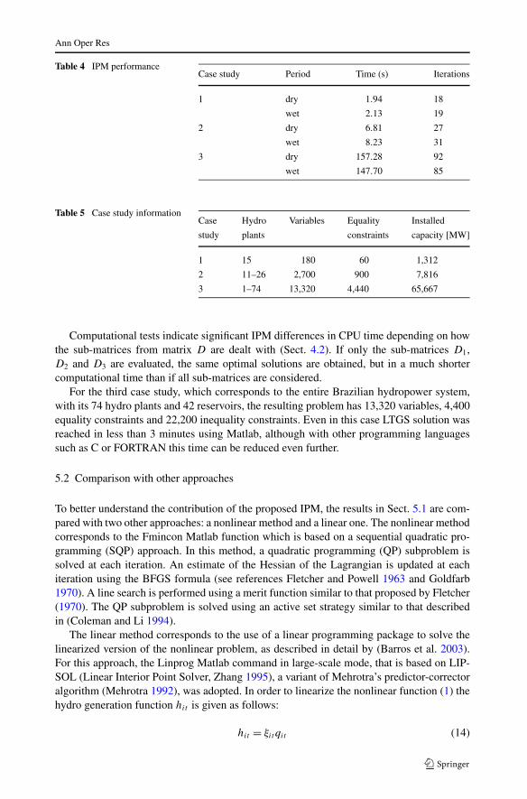
The computation time for all of these case studies is shown in Table 4, as well as thenumber of iterations necessary. In general, the computation time and the number of iterations

Ann Oper Res
Fig. 9 Generation trajectory ofGrande River hydro systemduring the wet period
Fig. 10 Generation trajectory ofthe Brazilian HydropowerSystem during the dry period
Fig. 11 Generation trajectory ofthe Brazilian HydropowerSystem during the wet period
for the wet period are greater than for dry period, since optimal solutions involving spillageare more difficult to establish than those without it.
Table 5 shows the number of hydro plants considered in each case study and the corre-sponding hydro scheduling problem dimensions.
Ann Oper Res
Table 4 IPM performanceCase study Period Time (s) Iterations
1 dry 1.94 18
wet 2.13 19
2 dry 6.81 27
wet 8.23 31
3 dry 157.28 92
wet 147.70 85
Table 5 Case study informationCase Hydro Variables Equality Installed
study plants constraints capacity [MW]
1 15 180 60 1,312
2 11–26 2,700 900 7,816
3 1–74 13,320 4,440 65,667
Computational tests indicate significant IPM differences in CPU time depending on howthe sub-matrices from matrix D are dealt with (Sect. 4.2). If only the sub-matrices D1,D2 and D3 are evaluated, the same optimal solutions are obtained, but in a much shortercomputational time than if all sub-matrices are considered.
For the third case study, which corresponds to the entire Brazilian hydropower system,with its 74 hydro plants and 42 reservoirs, the resulting problem has 13,320 variables, 4,400equality constraints and 22,200 inequality constraints. Even in this case LTGS solution wasreached in less than 3 minutes using Matlab, although with other programming languagessuch as C or FORTRAN this time can be reduced even further.
5.2 Comparison with other approaches
To better understand the contribution of the proposed IPM, the results in Sect. 5.1 are com-pared with two other approaches: a nonlinear method and a linear one. The nonlinear methodcorresponds to the Fmincon Matlab function which is based on a sequential quadratic pro-gramming (SQP) approach. In this method, a quadratic programming (QP) subproblem issolved at each iteration. An estimate of the Hessian of the Lagrangian is updated at eachiteration using the BFGS formula (see references Fletcher and Powell 1963 and Goldfarb1970). A line search is performed using a merit function similar to that proposed by Fletcher(1970). The QP subproblem is solved using an active set strategy similar to that describedin (Coleman and Li 1994).
The linear method corresponds to the use of a linear programming package to solve thelinearized version of the nonlinear problem, as described in detail by (Barros et al. 2003).For this approach, the Linprog Matlab command in large-scale mode, that is based on LIP-SOL (Linear Interior Point Solver, Zhang 1995), a variant of Mehrotra’s predictor-correctoralgorithm (Mehrotra 1992), was adopted. In order to linearize the nonlinear function (1) thehydro generation function hit is given as follows:
hit = ξit qit (14)

Ann Oper Res
Table 6 Comparison of methods for Furnas hydro plant in the dry and wet periods
Period Method Time (s) Iterations Objective function
dry Linprog 0.19 14 1.436 × 10⁸
Fmincon 535.88 219 1.018 × 10⁸
IPM 1.94 17 1.018 × 10⁸
wet Linprog 0.14 12 3.309 × 10⁷
Fmincon 474.81 219 1.585 × 10⁷
IPM 1.69 18 1.585 × 10⁷
The productivity ξit is now considered a fixed parameter instead of being a function ofthe decision variables, as considered in the formulation (1)–(6) where:
ξit = ki
(φi
(rit + rit−1
2
)− θi(qit + vit ) − ςi(qit )
)(15)
This linearization procedure has been adopted by (Barros et al. 2003; Medina et al. 1999;Ponnambalam et al. 1992). In (Barros et al. 2003) the average productivity obtained fromthe long-term operational records has been used as the fixed value of ξit . Here, the averageproductivity is calculated using the nonlinear solution given by the proposed IPM for eachof the case studies.
The next step in the linearization procedure of the LTGS model consists in the use of thefollowing objective function:
MinT∑
t=1
∣∣∣∣∣Dt −N∑
i=1
ξit qit
∣∣∣∣∣ (16)
which is equivalent to:
Minγt≥0
T∑
t=1
γt (17)
subject to
−γt ≤ Dt −N∑
i=1
ξit qit ≤ γt (18)
Equations (17)–(18) together with (2)–(6) correspond to the linearized model.Table 6 shows the results for the case study with Furnas hydro plant using the linear
model (Linprog), the nonlinear model (Fmincon), and the proposed IPM. It can be seenthat the proposed IPM achieves the same final value of the objective function achieved bythe Fmincon method in a much faster way (280 times). One of the reasons for this savingsin CPU time is the sparsity exploitation specially developed for the LTGS problem by theproposed IPM, as detailed in Sect. 4.2.
Another important result from Table 6 is that the linear model gave a quite worst finalobjective function value compared with the nonlinear models. This difference shows thatthe linearizations of the hydropower generation function, done by (14), and the objectivefunction, done by (16), lead to a great simplification of the model. Indeed, as shown in

Ann Oper Res
Fig. 12 Linear and nonlinearstorage trajectories for Furnashydroplant during the dry period
Fig. 13 Linear and nonlineargeneration trajectories for Furnashydroplant during the dry period
Fig. 14 Linear and nonlinearstorage trajectories for Furnashydroplant during the wet period
Figs. 12, 13, 14 and 15, the linear model provides a solution which produces lower storagetrajectories and much more unstable generation trajectories. With lower storages, the hydroplant operates with lower productivity, producing less hydropower generation for the same

Ann Oper Res
Fig. 15 Linear and nonlineargeneration trajectories for Furnashydroplant during the wet period
Table 7 Comparison of methods for the Grande River cascade during the dry and wet periods
Period Method Time (s) Iterations Objective function
dry Linprog 1.28 21 4.071 × 10⁹
Fmincon – – –
IPM 7.55 28 2.993 × 10⁹
wet Linprog 5.07 78 4.759 × 10⁸
Fmincon – – −IPM 7.25 29 3.363 × 10⁸
water discharge. Moreover, with more unstable generation, the monotonically increasingobjective function of (1) will provide higher values.
The linear and nonlinear models have also been compared for the Grande River cascadecase study and the results are presented in Table 7. For this case study, the Fmincon methodwas not able to solve the nonlinear model due to the fact that this method do not exploitthe sparsity as the developed IPM. As a consequence, the Fmincon, which requires a largeamount of memory, cannot be used. As shown in Table 7, the proposed IPM provides bettersolutions than Linprog in a small additional amount of computational time. Similar to thecase of Furnas hydro plant, the differences on objective function values are due to differ-ences on reservoir and generation trajectories. Figures 16 and 17 show the differences ongeneration trajectories between the linear and nonlinear models.
Finally, Table 8 presents the results for the Brazilian hydropower system. Here again thesame behavior of the Grand river cascade case is observed. The differences on the objectivefunction values are due to differences on operation as shown in Figs. 18 and 19.
The comparisons with other approaches have shown that linear models cannot adequatelycope with the nonlinear characteristics of the LTGS problem since they provide higher op-erating costs due to lower reservoir trajectories (lower productivity) and more unstable gen-eration trajectories. On the other hand, nonlinear approaches would require an adequatesparsity exploitation in order to cope with large-scale hydrothermal systems.

Ann Oper Res
Fig. 16 Linear and nonlineargeneration trajectories for theGrande River cascade during thedry period
Fig. 17 Linear and nonlineargeneration trajectories for theGrande River cascade during thewet period
Table 8 Comparison of methods for the Brazilian hydropower system during the dry and wet periods
Period Method Time (s) Iterations Objective function
dry Linprog 31.48 76 1.584 × 10¹¹
Fmincon – – –
IPM 140.91 92 1.283 × 10¹¹
wet Linprog 41.31 101 4.631 × 10¹⁰
Fmincon – – –
IPM 147.03 86 3.842 × 10¹⁰
6 Conclusion
This paper has presented an interior point method for long-term generation scheduling oflarge-scale hydrothermal systems. The problem was formulated and solved using an interiorpoint method as a nonlinear programming model which allows precise representation ofhydropower output and operational cost functions.

Ann Oper Res
Fig. 18 Linear and nonlineargeneration trajectories for theBrazilian hydropower systemduring the dry period
Fig. 19 Linear and nonlineargeneration trajectories for theBrazilian hydropower systemduring the wet period
The method was applied in three different case studies. In the first, composed of a singlehydro plant, a detailed analysis of the optimal solution is revealed. The second was com-prised of 15 hydro plants located in a single cascade, while the third involved 74 hydroplants in the Brazilian hydropower system. A planning period of 5 years and two differenthydrological scenarios (dry and wet years) were considered for numerical evaluations.
Comparison with a linearized and a nonlinear model were performed. The results attest tothe adequacy and efficiency of the proposed method for long-term scheduling of large-scalehydrothermal power systems.
References
Adler, I., Karmarkar, N., Resende, M. G. C., & Veiga, G. (1989). An implementation of Karmarkar’s algo-rithm for linear programming. Mathematical Programming, 44, 297–335.
Altman, A., & Gondzio, J. (1999). Regularized symmetric indefinite systems in interior point methods forlinear and quadratic optimization. Optimization Methods and Software, 11(12), 275–302.
Aravanitidis, N. V., & Rosing, J. (1970). Composite representation of a multireservoir hydroelectric powersystem. IEEE Transactions on Power Apparatus and Systems, PAS-89(2), 327–335.
Barros, M., Tsai, F. T. C., Yang, S.-L., Lopes, J.E.G., & Yeh, W. W. G. (2003). Optimization of large-scalehydropower system operations. Journal of Water Resources Planning and Management, 129(3), 178–188.
Bellman, R. (1962). Dynamic programming. Princeton: Princeton University Press.

Ann Oper Res
Benson, H., Shanno, D., & Vanderbei, R. (2000). Interior point methods for nonconvex nonlinear program-ming: Jamming and comparative numerical testing. Technical report ORFE-00-02, Operation Researchand Financial Engineering, Princeton University. http://www.princeton.edu/~rvdb/ps/loqo3_5.pdf.
Carvalho, M., & Soares, S. (1987). An efficient hydrothermal scheduling algorithm. IEEE Transactions onPower Apparatus and Systems, PWRS-2(3), 537–542.
Christoforidis, M., Aganagic, M., Awobamise, B., Tong, S., & Rahimi, A. F. (1996). Long-term/mid-term re-source optimization of a hydro-dominant power system using interior point method. IEEE Transactionson Power Apparatus and Systems, 11(1), 287–294.
Coleman, T., & Li, Y. (1994). On the convergence of reflective newton methods for large-scale nonlinearminimization subject to bounds. Mathematical Programming, 67(2), 189–224.
Dembo, R. S. (1991). Scenario optimization. Annals of Operations Research, 30(1), 63–80.Dikin, I. I. (1967). Iterative solution of problems of linear and quadratic programming. Soviet Mathematics.
Doklady, 8(1), 674–675.Escudero, L. F., a, J. L. G., & Pietro, F. J. (1996). Hydropower generation management under uncertainty via
scenario analysis and parallel computation. IEEE Transactions on Power Apparatus and Systems, 11(2),683–689.
Fletcher, R. (1970). A new approach to variable metric algorithms. Computer Journal, 13(1), 317–322.Fletcher, R., & Powell, M. (1963). A rapidly convergent descent method for minimization. Computer Journal,
6(1), 163–168.Gagnon, C. R., Hicks, R. H., Jacoby, S. L. S., & Kowalik, J. S. (1974). A nonlinear programming approach
to a very large hydroelectric system optimization. IEEE Transactions on Power Apparatus and Systems,6(1), 28–41.
Goldfarb, D. (1970). A family of variable metric updates derived by variational means. Mathematics of Com-puting, 24, 23–26.
Gondzio, J., & Sarkissian, R. (2003). Parallel interior point solver for structured linear programs. Mathemat-ical Programming, 96(3), 561–584.
Granville, S. (1994). Optimal reactive dispatch through interior point methods. IEEE Transactions on PowerApparatus and Systems, 9(1), 136–146.
Hanscom, M. A., Lansdom, L., & Provonost, G. (1980). Modeling and resolution of the medium term energygeneration planning problem for a large hydroelectric system. Management Science, 26(7), 659–668.
Karmarkar, N. (1984). A new polynomial-time algorithm for linear programming. Combinatorica, 4, 373–395.
Lyra, C., & Tavares, H. (1988). A contribution to the midterm scheduling of large scale hydrothermal powersystems. IEEE Transactions on Power Apparatus and Systems, 3(3), 852–857.
Martinez, L., & Soares, S. (2002). Comparison between closed-loop and partial open-loop feedback controlpolicies in long term hydrothermal scheduling. IEEE Transactions on Power Apparatus and Systems,17(2), 330–336.
Medina, J., Quintana, V., & Conejo, A. (1999). A clipping-off interior-point technique for medium-termhydro-thermal coordination. IEEE Transactions on Power Apparatus and Systems, 14(1), 266–273.
Mehrotra, S. (1992). On the implementation of primal-dual interior point method. SIAM Journal on Opti-mization, 2(4), 575–601.
Nabona, N. (1993). Multicommodity network flow model for long-term hydrogeneration optimization. IEEETransactions on Power Apparatus and Systems, 8(2), 395–404.
Oliveira, A. R. L., Soares, S., & Nepomuceno, L. (2003). Optimal active power dispatch combining networkflow and interior point approaches. IEEE Transactions on Power Apparatus and Systems, 18(4), 1235–1240.
Oliveira, G. G., & Soares, S. (1995). A second-order network flow algorithm for hydrothermal scheduling.IEEE Transactions on Power Apparatus and Systems, 10(3), 1652–1641.
Pereira, M. V. F., & Pinto, L. M. V. G. (1991). Multi-stage stochastic optimization applied to energy planning.Mathematical Programming, 52(2), 359–375.
Ponnambalam, K. (2002). Optimization in water reservoir systems. In P. M. Pardalos & G. C. M. Mauricio(Eds.), Handbook of applied optimization (pp. 933–943). Oxford: Oxford University Press.
Ponnambalam, K., Quintana, V. H., & Vanelli, A. (1992). A fast algorithm for power system optimizationproblems using an interior point method. IEEE Transactions on Power Apparatus and Systems, 7(2),659–668.
Quintana, V. H., Torres, G. L., & Medina-Palomo, J. (2000). Interior-point methods and their applicationsto power systems: Classification of publications and software codes. Operations Research, 29(4), 763–785.
Rosenthal, R. E. (1981). A nonlinear network flow algorithm for maximization of benefits in a hydroelectricpower system. Operations Research, 29(4), 763–785.

Ann Oper Res
Saad, M., Birgas, P., Turgeon, A., & Duquette, R. (1996). Fuzzy learning decomposition for the schedulingof hydroelectric power systems. Water Resources Research, 32(1), 179–186.
Sjvelgren, D., Anderson, S., Anderson, T., Nyberg, U., & Dillon, T. S. (1983). Optimal operations planning ina large hydro-thermal power system. IEEE Transactions on Power Apparatus and Systems, PAS-102(11),3644–3651.
Soares, S., & Salmazo, C. T. (1997). Minimum loss predispatch model for hydroelectric power systems. IEEETransactions on Power Apparatus and Systems, 12(3), 1220–1228.
Torres, G. L., & Quintana, V. H. (1998). An interior-point method for nonlinear optimal power flow usingvoltage rectangular coordinates. IEEE Transactions on Power Apparatus and Systems, 13(4), 1211–1218.
Turgeon, A. (1980). Optimal operation of multireservoir systems with stochastic inflows. Water ResourcesResearch, 16(2), 275–283.
Valdes, J. B., Filippo, J. M. D., Strzepek, K. M., & Restrepo, P. J. (1995). Aggregation-disaggregation ap-proach to multireservoir operation. ASCE Journal of Water Resource Planning Management, 121(5),345–351.
Wright, S. J. (1996). Primal-dual interior-point methods. Philadelphia: SIAM.Yan, X., & Quintana, V. H. (1997). An efficient predictor-corrector interior point algorithm for security-
constrained economic dispatch. IEEE Transactions on Power Apparatus and Systems, 12(2), 803–810.Zhang, Y. (1995). Solving large-scale linear programs by interior-point methods under the Matlab environ-
ment. Technical Report TR96-01, Department of Mathematics and Statistics, University of Maryland,Baltimore County, Baltimore, MD.