SUOMEN GEODEETTISEN LAITOKSEN JULKAISUJA VERÖFFENTLICHUNGEN DES FINNISCHEN GEODÄTISCHEN INSTITUTES

PUBLICATIONS OF THE FINNISH GEODETIC INSTITUTE ============================================ N:o 144 ============================================

INTERFERENCE MEASUREMENTS

OF THE NUMMELA STANDARD BASELINE

IN 2005 AND 2007

by

Jorma Jokela and Pasi Häkli

KIRKKONUMMI 2010

ISBN-13: 978-951-711-282-6 (printed) ISBN-13: 978-951-711-283-3 (PDF) ISSN: 0085-6932

3

Contents

Abstract ................................................................................................................. 4

1 Introduction ...................................................................................................... 5

2 Landmarks in the history of the Nummela Standard Baseline ......................... 8

2.1 First international recognitions ................................................................... 8

2.2 Change from invar wires to EDM instruments as transfer standards.......... 8

2.3 Recent construction works ........................................................................ 10

2.4 Importance in the 2010s ............................................................................ 13

3 Traceability chain of geodetic length measurements ..................................... 14

4 Quartz gauges in the determination of the scale ............................................ 16

4.1 Review of quartz gauge systems at Tuorla Observatory ........................... 16

4.2 Comparisons at Tuorla Observatory ......................................................... 17

4.3 Determination of the length of quartz gauge no. VIII in BTM00 ............. 21

5 Preparing the baseline for interference measurements................................... 24

5.1 Principle of the Väisälä interference comparator ...................................... 24

5.2 Preparing the observation pillars for interference measurements ............. 25

5.3 Precise levellings – start of the measurements.......................................... 25

5.4 Aligning the mirrors .................................................................................. 27

5.5 Setting the mirrors at correct positions in the baseline direction .............. 28

5.6 Installing the transferring bars onto the observation pillars ...................... 31

5.7 Installations on the telescope pillar ........................................................... 32

5.8 Installations on pillars 0 and 1 .................................................................. 35

6 Interference observations ............................................................................... 36

6.1 Observation procedure .............................................................................. 36

6.2 About weather conditions ......................................................................... 41

6.3 Personnel ................................................................................................... 43

7 Determination of corrections ......................................................................... 44

7.1 Compensator corrections .......................................................................... 44

7.2 Refraction correction ................................................................................ 45

7.3 Corrections due to mirrors ........................................................................ 49

7.4 Geometric corrections ............................................................................... 49

7.5 Projection corrections ............................................................................... 51

8 Computation of baseline lengths .................................................................... 58

8.1 Computation of the actual length of the quartz gauge .............................. 58

8.2 Results from interference observations in 2005 ........................................ 61

8.3 Results from interference observations in 2007 ........................................ 68

8.4 Final lengths .............................................................................................. 77

9 Estimation of uncertainty of measurement .................................................... 78

9.1 Combined uncertainty of the lengths between the underground markers . 78

9.2 Some supplementary analysis of uncertainty of measurement ................. 80

10 Summary and conclusions ........................................................................... 82

References ........................................................................................................... 84

4

Abstract

The Nummela Standard Baseline of the Finnish Geodetic Institute is a unique national and international measurement standard for length measurements in geodesy. The design of the 864-m baseline was originally, in 1933, fitted for the calibration of 24-m invar wires to determine a uniform scale for triangulation. Since 1947, the baseline has been regularly measured with the Väisälä interference comparator. As a continuation to the impressive time series, the performance and results of the latest interference measurements in 2005 and 2007 are presented in detail in this publication. Two consecutive measurements within a short time span were necessary, since only half of the baseline could be measured in 2005, due to unfavourable weather conditions. The new results again confirm the excellent stability and unique accuracy, 9×10-8, of the baseline. The 6-pillar baseline now serves in the calibration, testing and validation of electronic distance measurement (EDM) instruments for precise surveying and mapping and in scale transfer measurements to other geodetic baselines, test fields and local geodynamical networks. The measurements are metrologically traceable to the definition of the metre through a quartz gauge system.

This publication provides a summary of the rare measurement method and is a detailed supplement to the previously published or internal instruction manuals. First, we present the quartz gauge systems, which determine the scale in the Väisälä interference comparator. After a description of the present comparison method for the quartz gauges, the computation of the scale for the latest interference measurements is presented. For the interference measurements, the comparator must be separately constructed for every baseline. We describe the preparations and installations for this, followed by the observation and computation procedures. The abundant illustrations clarify the many stages. For further utilization of the baseline, the projection measurements are an essential part of the entire measurement. They transfer the distances between the mirror surfaces in the comparator to the distances between the permanently fixed transferring bars on the observation pillars, and, finally, to the baseline lengths between the underground benchmarks. We present the estimation of the uncertainty of measurement as standard and expanded uncertainties, combining all of the sources of the uncertainty in the traceability chain.

The standard uncertainties of the new results range from ±0.02 mm to ±0.07 mm for the lengths of the baseline sections ranging from 24 m to 864 m. The result for the length of the entire baseline, 864 122.86 mm ±0.07 mm, differs +0.11 mm from the previous result in 1996 and +0.08 mm from the first result in 1947. The largest difference between the results in 2005 and 2007 is –0.08 mm. The state-of-the-art Nummela Standard Baseline remains a world-class measurement standard of geodetic length metrology.

5

1 Introduction

The Nummela Standard Baseline of the Finnish Geodetic Institute (FGI), measured with the Väisälä interference comparator, is an internationally renowned measurement standard of geodetic length metrology. It offers calibration services in field conditions for the most accurate distance measurement instruments. During the era of triangulation, it mostly served in the calibration and determination of temperature coefficients for invar wires to produce a uniform scale for the field baselines for triangulation, and, thereby, for nationwide surveying and mapping. Later, it served in the calibration of electronic distance measurement (EDM) instruments. With EDM instruments, a traceable scale can be provided, for example to other geodetic baselines and test fields, or for scientific measurements, such as local control networks for possible crustal deformations or tie measurements at fundamental geodetic stations. The baseline is also used in the validation and testing of new instruments. International co-operation has been active during the long history of the baseline. The favourable environment and excellent stability enable accurate measurements with good reproducibility and repeatability, keeping the baseline in constant use.

In this publication we describe the unique measurement method and traceability chain from the definition of the metre to the lengths of the baseline sections in abundant details, which have not been documented before. Therefore, this publication may be a valuable supplement to the older published or internal instructions, covering both laboratory works on maintaining the quartz gauge system and field work on baseline measurements. Another major motivation for this publication is to serve the present clients of the baseline by publishing the results, the lengths with their uncertainties, of the newest interference measurements in 2005 and 2007.

Works for the Finnish first-order triangulation began already in 1919, and before 1933 a baseline in Santahamina, Helsinki, was used for determining the scale of the triangulation network. International compatibility of the fundamental measurements was ensured through comparisons with the invar wires used in other countries. The Nummela Standard Baseline was established in 1947, when the baseline, originally established with invar wire measurements in 1933, was measured with the Väisälä interference comparator for the first time. The latest measurement is no less than the 15th one, again with a 9×10-8 relative standard uncertainty for the entire length (864 m) of the baseline. Some events in the history of the baseline are treated in Section 2, including the recent remarkable construction works ameliorating working conditions and protecting baseline structures.

We present a brief summary of the traceability chain in Section 3, introducing the idea of scale transfer, that is, how the definition of the metre is transferred to lengths serviceable in present-day geodetic applications. This publication covers the middle parts of the traceability chain. It includes the maintenance of the quartz gauge system, the Väisälä interference comparator

6

and the Nummela Standard Baseline, and it excludes, in the beginning, the laboratory work with primary measurement standards and, in the end, the work with EDM instruments. References to the excluded parts are given in the text.

Quartz gauges, or quartz metres, are a set of measurement standards, which determine the scale for measurements with the Väisälä interference comparator. The lengths of some of them are determined in absolute calibrations using gauge block interferometers and monitored with regular comparisons to the principal normal, which are also based on interferometry. Section 4 reviews the different quartz gauge systems. The principal normal, quartz gauge no. 29, as well as most of the other quartz gauges, are stored in the Tuorla Observatory at the University of Turku. The FGI, as one of the only users of the quartz gauges these days, also essentially contributes to the maintenance of the quartz gauge system, but the absolute calibrations are commissioned to other metrological institutes. The 1-m-long quartz gauge no. VIII is always used in the Väisälä interference comparator at the Nummela Standard Baseline. The length of it, which is not constant, is known within a standard uncertainty of a few tens of nanometres.

We do not discuss in detail how to build a baseline for measurements with the Väisälä interference comparator in this publication. The basic requirement is evident: observation pillars or other foundations must be located in such places that the parts of the comparator can be installed on one line in space at a 1-mm-level. This sets strict constraints on baseline design, and only multiples of the lengths of the quartz gauges are allowed as suitable locations for observation pillars or mirrors. The baseline designs recommended for EDM calibration are, thereby, not practicable. Constructions on observation pillars must also have sufficient margins and adjusting mechanisms for the installation of the required instruments.

We describe in detail in Section 5 how to install the Väisälä interference comparator at an existing baseline. For a demonstration of indoor laboratory conditions, the installation for a “baseline” a few metres long is possible in one day. In field conditions the work is more challenging, and preparations on an array of pillars, up to nearly a distance of 1 km, usually take at least two weeks. After this, the centres of the mirrors should be on the same line in space and approximately at correct distances to enable the discovery of interference fringes. Also, the components for observing (light source, telescope, and so forth) must be adjusted, and the quartz gauge tuned to determine the scale. After this, the most interesting part of the measurement procedure awaits.

Finding interference fringes for short lengths is rather effortless after careful installations and adjustments. For long lengths, the procedure is often extremely laborious, and impeded by unfavourable weather conditions. We give advice for observations, learnt from experience, in Section 6. Once found, the fringes next time should be found using roughly the same adjustments. To eliminate questionable observations and ensure a reliable result, two observers participate in registering the interference fringes. This is essential, especially if the number of observations remains small.

7

Corrections to the observations are provided in Section 7, including a detailed description of the principle and the results of the projection measurements. Before utilizing the results from the interference observations, performed with temporarily installed adjustable equipment, they must be connected to something more permanent. At most standard baselines, underground sheltered benchmarks next to the observation pillars serve this purpose. The connection between the two arrays of observation points, from aboveground to underground, is realized in projection measurements. These theodolite-based, high-precision measurements are repeated during the entire two-three-month interference observation period. For calibrations of EDM instruments, reverse projection measurements from underground to aboveground are needed; then the observation pillars are equipped with forced-centring plates for surveying instruments instead of equipment from the Väisälä interference comparator.

The structure of this publication is also adapted to make the reader abundantly familiar with the computation of interference observations: the numerous but essential computation tables for the interference observations are provided sequentially in Section 8. First, we explain how the actual values of quartz gauge length, which were used to produce the scale of the latest interference measurements, were computed. After compensator and refraction corrections, the lengths between the mirrors’ surfaces are obtained. After a set of other corrections, these lengths are reduced to the lengths between underground markers. The final results consist of values attributed to the measurands (here, lengths of baseline sections) observed by measurement, and of the uncertainty parameters associated with them. We describe the estimation of uncertainty in Section 9. In this publication the term “length” is often used for a measurand, though the term “distance” would also be justified.

We present a comparison with previous results since 1947 in the short concluding Section 10. Since this publication is also intended to supplement the existing manuals on Väisälä baselines and the interference comparator, we include a large number of figures.

8

2 Landmarks in the history of the Nummela Standard Baseline

The first important turning point in the history of baselines in Nummela was in 1947, when invar wires, used at the comparison baseline since 1933, were replaced with the Väisälä interference comparator for the maintenance of the baseline. The history of the standard baseline began at this point. The Väisälä interference comparator had already been in use before this, but only for the lengths of the invar wires and not for the length of the entire baseline. Honkasalo (1950) documented the first interference measurements. Kukkamäki (1978) then presented a summary of the measurements performed by the FGI between 1947 and 1976. Some later important stages and turning points are listed in this section.

2.1 First international recognitions

Soon after the first interference measurements of the Nummela Standard Baseline, the Väisälä method received large international support. Activities for national and continental triangulations for surveying and mapping were most extensive at that time. In 1951, the International Association of Geodesy (IAG) made a motion in the General Assembly in Brussels, that “considering the high

accuracy obtained in the measurement of a standard base-line in Finland with a

light-interference apparatus, recommends that such bases be measured by a

similar method in different countries by the interested organizations and asks the

Bureau of the Association to facilitate necessary arrangements so that such

bases could be used, if desired, by neighbouring countries, to compare the

results obtained by this process, with those obtained by wires or tapes compared

to the standards of the International Bureau of Weights and Measures”. In 1954, the International Union of Geodesy and Geophysics (IUGG)

resolved in the General Assembly in Rome, that member countries should “establish a standard base-line in each country using the Väisälä method (or

similar apparatus) for assuring a uniform scale in all [triangulation] networks

and for calibrating invar tapes and geodimeters”. Since then, the Väisälä interference comparators have been delivered to more than ten countries. In addition, the Finnish Geodetic Institute measured baselines in more than ten countries: Finland (two baselines, 16 measurements, 1947–2007), Argentina (1953), The Netherlands (1957, 1969), Germany (West; four measurements in 1958–1963), Portugal (1962, 1978), DDR (1964), USA (1966), South Africa (1976), Spain (1978), Hungary (1987, 1999), China (two baselines, four measurements, 1985–1998) and Taiwan (1993).

2.2 Change from invar wires to EDM instruments as transfer standards

The importance of the Nummela Standard Baseline and its predecessors (comparison baselines in Santahamina until 1932 and in Nummela until 1947) is essential in determining the scale of the Finnish first-order triangulation. The invar wires, which since 1923 were used to measure the 16 field baselines for triangulation, were calibrated at those baselines. The lengths of the field

9

baselines ranged from 2.6 km to 6.2 km. The last one, the Finström baseline in Åland, was measured in 1966 (Kääriäinen 1984).

The 6.0-km-long Vihti field baseline, established in 1961, already served for the calibration of tellurometers as well; these were some of the first EDM instruments. The 22.2-km-long Niinisalo calibration baseline, measured with a large set of invar wires in 1968, was built especially for the calibration of EDM instruments (Kiviniemi 1970). The scale of these baselines was determined using measurements with invar wires calibrated at the Nummela baselines, but the use of both Vihti and Niinisalo baselines in calibrations for the Finnish first-order triangulation was eventually of minor importance. The numerous baselines established all over the country for the calibration of EDM instruments used in lower-order triangulations are not discussed here.

During the last years of triangulation, in addition to angle measurements, the FGI extensively performed trilateration. Distances were measured with a laser geodimeter (AGA Model 8) in northern Finland between 1971 and 1985 (Konttinen 1994). The modulation frequency of the instrument was measured twice a day, and the counter for that was compared with a quartz clock twice a year. Trilateration measurements, including geodimeter observations at the Niinisalo calibration baseline with an extension net, and of a 913-km-long traverse (Parm 1976), were included in the final adjustment of the Finnish first-order triangulation (Jokela 1994). In general, the scale of the geodimeter observations was not traceable to the Nummela Standard Baseline. This was reasonable, since the distances measured with the geodimeter (up to 70 km) were considerably longer than what was available for calibration at Nummela or Niinisalo, and the daily frequency control was an easy method for checking the instrument.

In practice, the scale of new nationwide distance measurements, performed especially in the Northern Finland, has not been derived from the Nummela Standard Baseline since the 1970s. However, the importance of the invar wire measurements, performed during the previous 50 years at the 16 field baselines all over the country, remained in the adjustments, which determined the scale of surveying and mapping in Finland. Only since the 1990s have new reference frames, based on completely different techniques, been introduced (yet with imperfect traceability).

Since the 1980s, national and international scale transfer measurements from the Nummela Standard Baseline have become common again, along with new high-precision medium-range EDM instruments, such as the Kern Mekometers ME3000 and ME5000. Now the scale transfer measurements mostly serve other geodetic baselines and test fields, for which a traceable scale is desired, and other scientific applications.

10

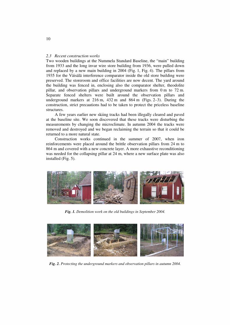
2.3 Recent construction works

Two wooden buildings at the Nummela Standard Baseline, the “main” building from 1933 and the long invar wire store building from 1936, were pulled down and replaced by a new main building in 2004 (Fig. 1, Fig. 4). The pillars from 1935 for the Väisälä interference comparator inside the old store building were preserved. The storeroom and office facilities are now decent. The yard around the building was fenced in, enclosing also the comparator shelter, theodolite pillar, and observation pillars and underground markers from 0 m to 72 m. Separate fenced shelters were built around the observation pillars and underground markers at 216 m, 432 m and 864 m (Figs. 2–3). During the construction, strict precautions had to be taken to protect the priceless baseline structures.

A few years earlier new skiing tracks had been illegally cleared and paved at the baseline site. We soon discovered that these tracks were disturbing the measurements by changing the microclimate. In autumn 2004 the tracks were removed and destroyed and we began reclaiming the terrain so that it could be returned to a more natural state.

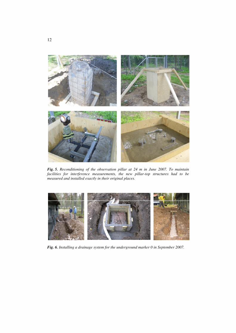
Construction works continued in the summer of 2007, when iron reinforcements were placed around the brittle observation pillars from 24 m to 864 m and covered with a new concrete layer. A more exhaustive reconditioning was needed for the collapsing pillar at 24 m, where a new surface plate was also installed (Fig. 5).

Fig. 1. Demolition work on the old buildings in September 2004.

Fig. 2. Protecting the underground markers and observation pillars in autumn 2004.

11

Fig. 3. The new shelter at the 864-m observation pillar and underground marker.

Fig. 4. The new office and store building at the Nummela Standard Baseline.

12

Fig. 5. Reconditioning of the observation pillar at 24 m in June 2007. To maintain

facilities for interference measurements, the new pillar-top structures had to be

measured and installed exactly in their original places.

Fig. 6. Installing a drainage system for the underground marker 0 in September 2007.

13

Originally, the observation pillars were built in 1946 for the first interference measurements, but the underground markers at 0 m, 432 m and 864 m had already been cast for the older comparison baseline. Pillars 0 and 1 were rebuilt in 1966 and the other pillars were reconditioned. The sheltering building with steel mesh walls and an aluminium plate roof was also built in 1966. It surrounds the observation pillars at 0 m, 1 m and 6 m and the telescope pillar. It has needed some reconditioning later. The underground markers at 24 m, 72 m and 216 m were cast as late as 1977.

At the underground marker 0, an underground drainage system was installed in 2007 to solve the long-time wetness problems there (Fig. 6). The first experiences are promising and one may even expect the 0.1 mm-level instability found in the projection measurements to be reduced.

2.4 Importance in the 2010s

At the beginning of the new millennium, the Nummela Standard Baseline is still used to transfer traceable scale in precise geodetic and geophysical measurements. Metrological comparisons for validating new measurement methods and instruments are another field of present applications.

Absolute long-distance measurements in the air are one new development trend in dimensional metrology, which are also prepared in a joint research project of the European Metrology Programme (EMRP) and partly funded by the European Commission. Here “long distances” refer to metrological long measurands, 1 m – 1 km. Nine European research institutes, including the FGI, are participating in the project, which lasts from 2008 to 2011. The aim is to develop new measurement techniques and instruments based on new technology. In the testing and validation of these new measurement techniques and instruments, the Nummela Standard Baseline as a world-class measurement standard may be of great importance. Utilizing it as a venue for an international comparison of high-precision distance measurement instruments has also been discussed. Official comparisons in this advancing field of research are still few. Some new scale transfer projects are also awaiting realization.

14

3 Traceability chain of geodetic length measurements

According to the current definition of the metre, agreed upon in the 17th General Conference on Weights and Measures (CGPM) in 1983, “the metre is the length

of the path travelled by light in vacuum during a time interval of 1/299 792 458

of a second”. Iodine-stabilized lasers are used as primary wavelength standards in the realization of this definition and in fundamental length measurements with laser interferometers. In the near future, new frequency comb techniques may be used in the realization of this definition.

Absolute calibrations with gauge-block interferometers for quartz gauges bring the absolute and traceable scale to the quartz gauge system in which the lengths of quartz gauges are given. Lassila et al. (2003) documents the latest absolute calibration. Rather laborious absolute calibrations are supplemented with more frequent comparison measurements in the maintenance of the quartz gauge system. Repeated measurements are necessary since the lengths of quartz gauges change slightly over time.

The Nummela Standard Baseline is one of the few geodetic baselines in the world maintained with regular measurements with the Väisälä interference comparator. These measurements transfer the traceable scale from the length of the quartz gauge to the baseline sections ranging from 24 m to 864 m, the latter obviously being close to the maximum range of operation of the comparator in the field conditions. The actual length of the quartz gauge during the measurements is determined using temperature and air pressure observations and multiplied using the comparator. The temporary locations of the mirrors in the comparator are registered relative to the transferring bars on the observation pillars, the lengths between which are hereby obtained. The lengths between the transferring bars are projected onto lengths between more stable underground benchmarks. The equipment installed on the observation pillars is different in interference measurements and in the calibration of EDM instruments, and reverse projection measurements from underground benchmarks to observation pillars are needed later for calibrations.

According to metrological terminology (BIPM 2008a), the quartz gauge system and the Nummela Standard Baseline can be regarded as secondary measurement standards. High-precision EDM instruments are used as transfer standards or working standards when transferring the traceable scale further to other geodetic baselines or applications. These instruments are calibrated at the standard baseline, where the scale correction and the additive constant of the instrument are determined by comparing the observed values with the “true” values from the interference measurements. Calibrations are usually performed both before and after the measurements at the baseline or geodetic network, to which the scale is transferred. The observed values always need velocity corrections due to weather conditions and often also geometric corrections due to height differences or horizontal non-parallelism. (It is more common to make a calibration of modulation frequency for an EDM instrument, but the method discussed in this publication provides a completely different and independent

15

traceability chain.) Most of the recent scale transfers have been made using Kern Mekometer ME5000 EDM instruments. There is a problem, however, in that these instruments are ageing and few other suitable instruments are available. Jokela et al. (2009 and 2010) document some recent scale transfer measurements which are already utilizing the new results from the latest interference measurements. The traceability chain is depicted in Fig. 7.

Typical combined standard uncertainties are 4×10-8 for the lengths of the quartz gauges, 1×10-7 for the standard baselines and from 2×10-7 to 5×10-7 for the lengths after scale transfer with an EDM instrument. These values are valid for an adequate number of observations and proper processing.

Fig. 7. Traceability chain of geodetic length measurements. This publication

concentrates on the second and third phases of the chain.

Definition of the metre

Quartz gauge system

− absolute calibrations

− relative comparisons

→ the lengths of the quartz gauges

Measurements with the Väisälä interference comparator

→ the length of the Nummela Standard Baseline

Calibration of a transfer standard at a standard baseline

→ the scale correction of the transfer standard,

a high-precision EDM instrument, such as Kern ME5000

Scale transfer measurements at another baseline

→ the traceable scale to another baseline or geodetic network

16

4 Quartz gauges in the determination of the scale

4.1 Review of quartz gauge systems at Tuorla Observatory

Traceability describes the property of a measurement result whereby the result can be related to a reference through a documented unbroken chain of calibrations, each contributing to the measurement uncertainty (BIPM 2008a). The scale of the Väisälä interference comparator is traceable to the definition of the metre, an SI unit, through a quartz gauge system, in which lengths of tens of quartz gauges (also known as quartz metres) are determined through repeated comparisons and absolute calibrations. The lengths do not remain unchanged; instead, a fairly regular, slow lengthening has been observed with most quartz gauges. Several systems have been used since 1933. In practice, introducing a new system means that the best possible new measurement results are used in computing the lengths: new or upgraded systems are needed after every absolute calibration. The review presented here is mostly based on the manuscripts by Niemi (2001 and 2005).

Yrjö Väisälä presented the interferometrical method for length measurements in his dissertation in 1923 (Väisälä 1923). He manufactured the first quartz gauges in 1927, when he was a professor of physics at the University of Turku. The most commonly used quartz gauges are 1-m-long, 23 mm thick hollow quartz tubes sealed with 10 to 15-mm-thick cylindrical ends, which are spherical with different radii of curvature; for special purposes, other dimensions and materials and flat-end gauges are available too.

In 1933, when 18 quartz gauges were available, T.J. Kukkamäki published their lengths and temperature and atmospheric pressure coefficients in his dissertation (Kukkamäki 1933). His dissertation also included a comparison with the Finnish platinum-iridium-prototype no. 5. In addition, Kukkamäki’s system (TKK) was compared with the German prototype of metre no. 18. The standard uncertainty of the first absolute measurement was ±300 nm, that is, 3×10-7; in relative comparisons, it was of the order of 1×10-8.

During the next years, researchers, including some of Väisälä’s students at the University of Turku, made more comparisons and initial applications for the geodetic baseline measurements. The purpose was to calibrate invar wires and tapes; also, an alternative quartz gauge system (LKL) was introduced in 1937 by M. Laaksokivi and S. Lekkala. In 1947, T.J. Kukkamäki and T. Honkasalo measured the 864-m Nummela baseline at the Finnish Geodetic Institute. It had already been used to transfer the scale to the triangulation and mapping of Finland since its establishment in 1933. Since 1947, the Nummela Standard Baseline has served not only Finnish geodesists; it has also served as a world-class length standard of geodetic metrology.

The quartz gauges are stored and compared in “Sauna”, a cave room inside the granite hill of Laukkavuori at the Tuorla Manor. This is the place where the University of Turku’s Tuorla Observatory was founded in 1952. Nowadays, the Tuorla Observatory, a division of the Department of Physics and Astronomy,

17

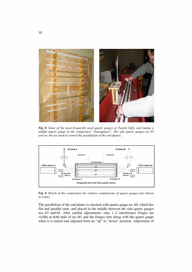
together with the Space Research Laboratory form the Väisälä Institute for Space Physics and Astronomy (VISPA) at the University of Turku. The name “Sauna” stands for the possibility to control temperature – the comparator is called “Saunapiano”, which is distinct from a set of string systems of the older “piano” comparators (Fig. 8).

The present principal normal of the quartz gauge system, quartz gauge no. 29, was made in 1953. Older comparisons have been tied to later systems using common quartz gauges for comparisons at different times. Even the definition of the metre has changed twice during the comparisons, in 1960 and in 1983. New absolute calibrations for some Finnish quartz gauges (nos. VIII and IX) at the BIPM (Bureau International des Poids et Mesures) in 1953 resulted in a new quartz gauge system (T, Terrien). These were the first absolute calibrations tied to the wavelength of light. Later absolute calibrations of quartz gauges (nos. 42 and 53, used in Germany) were made at the PTB (Physikalisch-Technische Bundesanstalt, Braunschweig, Germany) in 1964 (quartz gauge system E, Engelhard) and again at the BIPM in 1965. The incompatibility of the results both internationally and with the Tuorla system (K, Kukkamäki) prompted Väisälä and L. Oterma to improve the absolute calibration facilities at Tuorla (Väisälä and Oterma 1967). The results (for nos. 30 and 32) obtained in 1966 improved the reliability of the lengths of the Tuorla system. Later on, absolute calibrations were performed at the PTB in 1970 (nos. 42 and 53), 1978 (nos. 30, 49 and 51), 1993 (nos. 49 and 51) and 1995 (nos. 30, 49 and 51; PTB 1996), and, finally, at MIKES (Centre for Metrology and Accreditation, Helsinki, Finland) in 2000 (nos. VIII, 49, 50 and 51; MIKES 2000). The method used at MIKES is described in Lassila et al. (2003). Comparisons with the principal normal (no. 29) have been performed before and after every absolute measurement. The absolute calibrations at the PTB and MIKES and the comparisons at Tuorla determine the present quartz gauge system BTM00 (Braunschweig–Tuorla–MIKES 2000), which replaced the previous BT systems.

4.2 Comparisons at Tuorla Observatory

In the comparator box, two plane-convex lenses are adjusted parallel to one another at a distance of 1 001 mm (Fig. 9). The 1 mm shorter quartz gauges are adjusted horizontally on the supports between the plane surfaces. Outside the box, two Cd (cadmium) spectral lamps are used as light sources in the focal points of the lenses, and two CCD cameras are used for registering the images of the interference fringes. Part of the light reflects from the end plane and part of it reflects from the gauge end, producing interference fringes. The auxiliary parts include prisms, filters, screens and diaphragms to direct the light beam and thermometers for monitoring the temperature.

Before the comparison, the temperatures of the comparator room and the quartz gauges must be steady; the air-conditioning must be turned on at least one day beforehand. After every adjustment of the gauges, cooling of the temperatures typically continues for 10–20 minutes.

18

Fig. 8. Some of the most frequently used quartz gauges at Tuorla (left), and tuning a

middle quartz gauge in the comparator “Saunapiano”. The side quartz gauges no. 63

and no. 64 are used to control the parallelism of the end planes.

Fig. 9. Sketch of the comparator for relative comparisons of quartz gauges (not drawn

to scale).

The parallelism of the end planes is checked with quartz gauge no. 60, which has flat and parallel ends, and placed in the middle between the side quartz gauges nos. 63 and 64. After careful adjustments, only 1–2 interference fringes are visible at both ends of no. 60, and the fringes turn along with the quartz gauge when it is turned and adjusted from an “up” to “down” position. Adjustment of

19

the end planes is seldom needed. This check is performed before and after every comparison. Also, the positions of the side quartz gauges are checked and adjusted, if needed. The end planes and quartz gauges have aiming lines and markers to help in finding the correct positions. The comparator box has a set of adjusting screws (Fig. 10), and the positions can be viewed on the computer monitor (Fig. 11). During the comparison, the side quartz meters control the change between the end planes; the closing error, caused by uncertainty in the measurement and deformation, is typically ±40 nm. The quartz gauge to be measured or compared is adjusted in the middle of the side gauges and measured in the “up” and “down” positions.

Fig. 10. Most of the adjustments are made at the B-end of the comparator box.

Fig. 11. After turning quartz gauge no. VIII around on its axis (from the “up” to

“down” position, or vice versa), both vertical and horizontal adjustments are needed to

return the B-end to its proper position for taking pictures for the measurements.

20

Fig. 12. A picture of the B-end of quartz gauge no. VIII in the up position.

In every comparison the principal normal, quartz gauge no. 29, is measured first and last and the other quartz gauges are measured in between. The shorter than 1 mm distances between the ends of the quartz gauges and end planes are measured at both ends (A and B) and at the two gauge positions (up and down). The measurement of one quartz gauge in one position takes a few minutes, and the temperature should be stable within a few thousandths of a degree. Movement of the motorized cameras and the taking of pictures are controlled with the computer in the outer room (Fig. 12). Ten pictures are usually taken in the following order: A2, A1, A2, A3, A2, B2, B1, B2, B3, and B2. In this sequence, A and B stand for the comparator end, 1 and 3 are the side quartz gauges nos. 63 and 64, and 2 is the actual quartz gauge to be measured. More pictures may be necessary for problematic cases, such as the A-end of quartz gauge no. VIII with a short (1 m) radius of curvature. The processing of different pictures (A2, B2) should give the same result, with a standard deviation of the mean of about ±5 nm. Kukkamäki (1933, p. 15–47) describes in detail how to compute the distances between the ends of quartz gauges and end planes. Later modifications to the instrumentation and computation include changes in the light sources and camera systems and the use of computers. Nonetheless, the main principle has remained the same. When analyzing the pictures, the fraction part and the integer number of halves of the wavelength between the quartz gauge and the end plane are determined using four different wavelengths.

The distance between the end planes is determined from the approximate lengths of the side quartz gauges nos. 63 and 64 and the length of quartz gauge no. 29, with temperature (and pressure) corrections made to them, and from the measured gaps between the quartz gauges and the end planes. Using the average value of the lengths at the two side gauges removes the influence of possible

21

non-parallelism of the end planes in the middle. The length of another quartz gauge is determined by replacing quartz gauge no. 29 in the middle of the comparator with the other quartz gauge and subtracting the measured gaps at the end planes from the now known distance between the end planes.

4.3 Determination of the length of quartz gauge no. VIII in BTM00

With the present constellation of observation pillars, the only quartz gauge that can be used in the Väisälä interference comparator at the Nummela Standard Baseline is the exceptionally long quartz gauge no. VIII. For example, a 100 µm shorter quartz gauge would produce an 86.4 mm shorter baseline, demanding modified observation pillars. Quartz gauge no. XI has also been used until 1977, but not later, since the shape of it is slightly imperfect and inconvenient to use.

The length of quartz gauge no. VIII was determined in comparisons made at the Tuorla Observatory before and after the measurements at Nummela both in 2005 and in 2007. In these comparisons the principal normal, quartz gauge no. 29, was measured every day first and last, and no. VIII and a couple of other quartz gauges (no. 49 and no. 51) were measured in between. The principal normal, quartz gauge no. 29, is used in determining the distance between the end planes in the quartz gauge comparator.

The observed absolute length Labs of quartz gauge no. VIII is obtained from the measured length Lmeas by making a temperature correction to normal conditions and correcting the nominal length of the principal normal to the absolute value:

Labs,VIII,epoch = Lmeas,VIII,epoch –a(t–20) –b(t–20)2 –c(t–20)3 +Lcorr,29,epoch –L29 ,

where t is the temperature (°C), and the coefficients determined at the Tuorla Observatory (in the quartz gauge system BTM00) are a = 0.4003, b = 0.00141 and c = 0.0000605. L29 is the nominal length –100.550 µm (+1 m). The temperature correction makes the absolute length of quartz gauge no. VIII comparable with the principal normal. The corrected length Lcorr,29,epoch takes into account the lengthening of the principal normal after the reference epoch, to which the nominal length, based on previous absolute measurements and relative comparisons, is related.

Lcorr,29,epoch = p +q1[(epoch–1971)/(epoch–1956)] , if epoch ≥ 1971, or

Lcorr,29,epoch = p +q2(epoch–1971) , if epoch < 1971,

where p = –100.5314 µm (+1 m), q1 = 0.2818 and q2 = 0.02017 are constants determined in a polynomial fit of absolute calibrations and comparisons for BTM00. The years 1971 and 1956 are the reference epochs for the system. For epoch 2000, Lcorr,29,2000 = –100.3457 µm (+1 m).

The results from recent comparisons at the Tuorla Observatory are presented in Table 1. The comparisons were performed by Aimo Niemi (spring 2005), Joel Ahola (autumn 2007), Pasi Häkli (spring and autumn 2005 and spring 2007) and Jorma Jokela (all).

22

When utilizing the abundant absolute calibration (Fig. 13) and comparison data (Fig. 14) in the long time series, the calculated lengths can also be obtained fairly independently of the current measurement:

Lcalc,VIII,epoch = Lcalc,VIII,2000 +dL(epoch–2000) +Lcalc,29,epoch –Lcalc,29,2000 .

Lcalc,VIII,2000 = +151.3160 µm (+1 m) is the length of quartz gauge no. VIII at epoch 2000 in BTM00 and dL = +0.0027 µm a-1 is its annual change of length relative to the principal normal. The values Lcalc,29,epoch are listed in Table 1; Lcalc,29,2000 = –100.3457 µm (+1 m). The results are presented in Table 2.

Fig. 13. Length of the principal normal, quartz gauge no. 29, determined from absolute

calibrations at PTB, Tuorla and MIKES.

Fig. 14. The length of quartz gauge no. VIII from comparisons at Tuorla. The black spot

at 2000 signifies the absolute calibration of this particular gauge at MIKES.

When choosing the final length of quartz gauge no. VIII for the computations of measurements with the Väisälä interference comparator, either the calculated or the just measured values can be used. Generally, it is reasonable to pay attention to both of them. The latest absolute calibration at epoch 2000.2 gave the result 1.000 151 371 m with ±72 nm combined expanded uncertainty with the coverage factor k = 2 (MIKES 2000). Also, three of the other quartz gauges (nos. 49, 50, and 51) were then calibrated, which all contribute to BTM00.

-101,0

-100,5

-100,0

1950 1960 1970 1980 1990 2000 2010

µµµµm

+

1 m

Year

150,5

151,0

151,5

1950 1960 1970 1980 1990 2000 2010

µµµµm

+

1 m

Year

23

Table 1. The observed length Lmeas of quartz gauge no. VIII is reduced to absolute value

Labs with the temperature correction and when using the calculated length Lcalc,29 of

principal normal, quartz gauge no. 29. The lengths L are in µm (+ 1 m), and the

temperatures t in °C.

Epoch Lmeas, VIII t Lcalc,29 Labs, VIII

2005.282 +149.8143 16.790 –100.3354 +151.3014 2005.299 +149.9403 17.035 –100.3353 +151.3310

average 2005.290 +151.3162 2005.937 +150.2658 18.005 –100.3342 +151.2750 2005.937 +150.3520 18.110 –100.3342 +151.3197

average 2005.937 +151.2974 2007.236 +150.4775 18.290 –100.3321 +151.3761 2007.236 +150.4999 18.430 –100.3321 +151.3430

average 2007.236 +151.3596 2007.926 +150.4034 18.270 –100.3310 +151.3110 2007.926 +150.5587 18.355 –100.3310 +151.4326

average 2007.926 +151.3718

Table 2. The calculated length Lcalc of quartz gauge no. VIII, based on the time series

from 1953 to 2007.

Epoch Lcalc,VIII

2005.290 +151.3406 2005.937 +151.3435 2007.236 +151.3491 2007.926 +151.3521

From the average values of the spring and autumn measurements in 2005 (Table 1), the value +151.3014 µm (+1 m) is obtained for the mean epoch of interference measurements at Nummela, 2005.8. Respectively, the value +151.3696 µm (+1 m) is obtained for the mean epoch of the next interference measurements at Nummela, 2007.8. These are the results from measurements at Tuorla. The calculated values (Table 2) from the time series are +151.3429 µm (+1 m) for epoch 2005.8 and +151.3516 µm (+1 m) for epoch 2007.8. The conclusion is to use the average values of the measured and calculated values for processing the interference measurements at Nummela: the length of quartz gauge no. VIII in standard conditions (t = 20 °C, P = 760 mmHg) was 1.000 151 322 m at epoch 2005.8 and 1.000 151 361 m at epoch 2007.8. The length of gauge no. VIII during each interference measurement at the Nummela Standard Baseline can be computed from these values by correcting the standard length to the actual length during the observations with temperature and atmospheric pressure corrections, see Section 8.1.

24

5 Preparing the baseline for interference measurements

5.1 Principle of the Väisälä interference comparator

The design of the Nummela Standard Baseline was originally adapted for the calibration of 24-m-long invar wires. The entire length, 36 x 24 m = 864 m, was equipped with wooden stands at every 24 m between the underground markers at 0 m, 432 m and 864 m. These underground markers are brass bolts cast in concrete pillars and covered with small concrete blocks and wooden boxes in the ground. In the design for measurements with the Väisälä interference comparator, a longer length is always a multiple of a shorter length. This was realized up to 864 m using several multiplications: 2 x 2 x 3 x 3 x 4 x 6 x 1 m = 864 m. The observation pillars were cast at the intermediate and end points at 864 m, 432 m, 216 m, 72 m, 24 m, 6 m, 1 m and 0 m. This line was placed about 2 m away from the line between the underground markers. The heights of the observation pillars are 0.7 m to 1.4 m from the ground, and the depths are 0.8 m, except for the especially wide pillar 0–1, which is only 0.3 m deep (Honkasalo 1950). The underground markers extend to a depth of 2 m.

There are a few publications, for example by Kukkamäki (1969) and Jokela and Poutanen (1998), which describe in detail how to install the Väisälä interference comparator on the observation pillars and how to use it. The principle is shortly revised here, and more details are presented in the next pages.

In the comparator (Fig. 15), the white light from a point-like source is made parallel with a collimator lens and divided into two beams. One part of the light travels between the front mirror and the middle mirror, the other part travels to and from the back mirror. The distance between the front and back mirrors is an integer multiple n of the distance between the front and middle mirrors. The light beam travels n times between the first two mirrors, and once to and from the back mirror. The mirrors are adjusted in such a way that the two beams, travelling different paths, but equal distances, meet at the focal plane of the observing telescope. The light source and the telescope include fine-mechanical and optical components to control the light beams, whereas the structures of the other parts of the comparator are very simple. The reflections are directed to the telescope with the numerous adjustment screws for mirrors. The final adjustment of the incoming beams with adequate accuracy is made with the screen and the compensator glasses in front of the telescope.

The observations include: (1) registering of the mirror positions relative to the permanently fixed transferring bars on the observation pillars; (2) the rotation angles of the compensator glasses, leading to compensator corrections; (3) measuring the shortest interference with the quartz gauge, which is somewhat more complicated; and, (4) temperature observations, which accompany every interference observation. The transfer readings in item (1) are taken last, after all observations for the shorter interferences have been made and before the mirrors are removed for longer interferences. For further utilization,

25

the positions of the transferring bars (and mirrors) relative to the underground markers are determined in projection measurements, which are repeated several times during the interference measurement period.

Fig. 15. The principle of the Väisälä interference comparator and the geometry of the 0–

6–24-interference (not drawn to scale, reprint from Jokela and Poutanen 1998).

5.2 Preparing the observation pillars for interference measurements

The observation pillars are usually equipped with forced centring-plates for calibration measurements. They are fixed onto heavy iron plates, which are then fixed onto the observation pillars. The plates cannot be used with the Väisälä interference comparator. When removing them, it is advisable to record their old exact locations on the iron stands emerging from the observation pillars. This helps when installing the plates again after the interference measurements, since the space on the supports for making adjustments is very limited and all the plates should, again, be about on the same line in space. Broken threads or nuts for fixing screws in the pillars are replaced, where needed, and rusty parts are polished and painted. Visibility between the pillars is cleared by removing disturbing vegetation.

5.3 Precise levellings – start of the measurements

Measurements are begun with precise levellings (Fig. 16). Height differences are needed to install the components of the Väisälä interference comparator on the same line in space, and to reduce the resulting slope lengths to a preferred reference height level.

At the old baselines, the height differences are known from previous measurements and possible small changes are insignificant in the determination of height reductions. Levelling is still recommended, since it is a precise measurement method that easily reveals possible instability. Tenths of a millimetre differences are acceptable, since all benchmarks have not rounded but flat tops, which are not optimal for levelling. A Zeiss DiNi12 digital level and two bar code rods were used for the precise levellings in 2005 and 2007. The digital levelling instrument and rods are regularly calibrated at the FGI’s system calibration comparator.

Line between underground markers

Line between mirror centres

Light source Collimator lens

Mirror 0 Mirror 6 Mirror 24

Theodolite

Telescope

26

Fig 16. Arrangements for precise levellings with a Zeiss DiNi12 digital level and two

bar code rods. The height differences between the underground markers are levelled

first, both to and fro. The height differences between the underground markers and the

reference points on the observation pillars are levelled next. Common levelling

accessories and auxiliary pillars are used as intermediate points. Rulers or homemade

bar code rods may be needed to determine the heights of the observation instruments.

27

Fig. 17. Curvature of the Earth, R = 6 370 km. At 432 m the line in space between

mirror centres 0 and 864 goes 14.6 mm lower than the levelled height. For shorter

lengths, the correction is 10.9 mm at 216 m, 4.4 mm at 72 m, 1.5 mm at 24 m, and

0.4 mm at 6 m.

The height differences between underground markers are determined first, both to and fro. After this, one point is levelled on every observation pillar relative to the corresponding underground marker; a point on pillar 0 may also serve levellings for pillars 1 and 6 and the telescope pillar. The levelled points are later used in adjusting and mounting all parts of the comparator at the correct heights. The heights of end points 0 and 864 are fixed, and everything else is fitted on the same sloping line. The curvature of the Earth must not be forgotten; for example, at 432 m the straight line goes 14.6 mm lower than what levellings along an equipotential surface would suggest (Fig. 17).

Another detail is that at the 0-end of the baseline all instruments must be slightly inclined, according to the slope of the baseline (about 0.309 gon). Height references on the observation pillars are used in the levellings for mirror rails, supports and centres. A short (1.2 m) wooden rod, a measurement tape or a ruler were used as a rod, and the Wild N3 level was used in addition to digital levelling. In adjusting the heights, pieces of aluminium plate are often needed between the iron supports and the mirror rail stands to raise the height of the instruments, or some screws must be shortened or changed to longer ones. At a new baseline, this can be eliminated by careful planning and construction of the observation pillars.

The results of the precise levellings and the corrections determined from them are presented in Section 7.4.

5.4 Aligning the mirrors

The most accurate theodolite available should be used in aligning the mirror centres along the same line in space. In this instance, we used a Kern DKM3, which we placed on the theodolite pillar along the continuation of the baseline, about 20 metres behind the 0-pillar (Fig. 18). The final position of the theodolite and the centre of mirror 864 determine the line upon which the other mirror centres are adjusted. When the final position is chosen, one should make sure that there is enough room left to adjust the mirrors on every pillar. The position of the theodolite is marked on the theodolite pillar. At this point, the theodolite is

864 0

R R

y

x

432

28

kept under cover during the entire measurement period. It can later be used to find the correct positions of the mirrors if some of them get badly directed so that a reflection is completely lost.

Using the theodolite, we first adjust the mirror rails on the line (Fig. 19). We direct the aimings to the front and back screws of the mirror rails (or to clearly visible targets placed on them), and correct the positions of the rails as necessary. In spite of using a precise instrument, it is important always to read the angles at the two theodolite face positions. The mirror rails are also levelled horizontally (along and across the baseline) and adjusted and fixed at the correct height. When the mirror rails are in the correct positions (usually after a few days effort) it should be quite easy to install the mirror centres along the same line, again by observing with the theodolite the constant direction to the mirror centres. At the distant mirrors, visibility can be improved by illuminating the mirrors from behind with a torch.

It is more difficult to turn the mirrors in the correct positions exactly perpendicular to the line of sight, so that a reflection from the telescope returns back to the telescope. In order to first approximately find the reflection, a hand-held torch is useful, especially for the longest lengths. The torch can be used to direct the mirror perpendicular to the baseline by first adjusting the mirror with the torch reflection close to the mirror and then repeating the procedure while moving farther away from the mirror (and thus approaching the theodolite). The final adjustments are done with the theodolite. A small battery-operated lamp is permanently fixed in front of the theodolite objective to help with the final tuning. The light reflecting from the centre of mirror 864 is first directed to the hair cross of the telescope, and then reflections of other mirror centres are directed to the same point. The mirror centres must be adjusted both vertically and horizontally along the same line within about 1-mm accuracy, before the mirrors can by successfully directed.

5.5 Setting the mirrors at correct positions in the baseline direction

Before doing a search of the interference fringes, the mirrors must also be at correct positions in the baseline direction, again preferably within 1 mm. This can be measured and adjusted using a precise tacheometer and a prism reflector, which is placed above a mirror (freehand, since it may be difficult to fix), and similarly above every mirror to be measured. The tacheometer is set up behind the telescope along the continuation of the baseline. To prevent disturbing extra reflections, the reflecting mirror surfaces of the comparator must be covered during the EDM observations. The multiplied length of the quartz gauge determines the correct positions; later, the already found shorter interferences can give the scale for the measurement. The distant mirror is always moved to a proper distance by using the front and back screws of the mirror rail. One rotation of the screws moves the mirror stand 1 mm. The thickness of the front mirror must be taken into account, since the distances between the reflecting surfaces are determined.

29

Fig. 18. Kern DKM3 theodolite with an autocollimation lamp on the theodolite pillar.

Fig. 19. Mirror equipment: (1) mirror rail, (2) mirror stand and (3) mirror in its frame,

above a transferring bar and on three iron supports on an observation pillar. First, the

rail is levelled and adjusted to the correct height (4, three screws). After the correct

position of the mirror rail is found, it is permanently fixed to the observation pillar (5,

one screw). The transferring bar (6) is equipped with a collar ring, which directs the

probing point of the transferring device to the centre of the mirror (see also Fig. 21).

The mirror stand can be moved along the rail in the direction of the baseline (7, two

screws) and the mirror in its frame can be tilted in its stand (8, six screws). The mirror

frame can also be moved or straightened in a direction perpendicular to the baseline (9,

two screws). The targets (10, as a distant mirror, or 11, as a mirror to be projected)

serve in the projection measurements.

30

Fig. 20. Using previous results X for setting mirrors at approximately the correct

positions in the baseline direction. X are lengths of baseline sections between

underground markers from previous measurements. M are distances between mirror

surfaces in the interference position. P are projection corrections between underground

markers and mirror centres. L are transfer readings between transferring bars and

mirror surfaces.

At the old Väisälä baselines with known lengths, the previous results can be very useful in finding the interference fringes again. Of course, this has no influence on the new results. The method is presented here (Fig. 20) and was successfully applied to searching for the 864 m interference in 2007. The previous results were from the lengths of baseline sections, 432 m and 864 m, between the underground markers in the interference measurements taken in 1996.

When a shorter interference, 432 m, had been found, mirrors 0, 216 and 432 were at definite positions; also, the quartz gauge was already being used to determine the exact scale. Using the new projection corrections P at pillars 0 and 432, the difference of transfer readings L between the interference positions and the projection positions, and the approximate thicknesses D of the mirrors, 20 mm, it was possible to compute the distance M1 between mirror surfaces 0 and 432 by assuming the known length between underground markers 0 and 432, unchanged from 1996, X1 = 432 095.36 mm:

M1 = X1 –P432 –½D –LP

432 +LI432 –P0 –½D –L

P0 +L

I0 .

Here, the projection corrections P432 = 16.97 mm and P0 = 0.83 mm, and the transfer readings L

P432 = 14.21 mm and L

P0 = 11.40 mm, are from projection

measurements, and the transfer readings LI432 = 14.86 mm and L

I0 = 11.43 mm

M1

M2

L0

L432

L864

P432

P864

X1

X2

864

432

0

P0

31

are related to the interference position. From these values, the distance M1 = 432 058.24 mm is obtained.

The distance between mirror surfaces 0 and 864 in the interference position is a multiple of this shorter distance, M2 = 2M1 = 864 116.48 mm. Using X2 = 864 122.75 mm from 1996, and P864 = 24.07 mm, P0 = 0.83 mm, L

P864 = 21.87 mm and L

P0 = 11.40 mm from projection measurements, an

estimate for the transfer reading LI864 in interference position is obtained:

LI864 = M2 –X2 –P864 +½D +L

P864 +P0 +½D +L

P0 –L

I0 .

The plus and minus signs in the formulas are not always applicable, but they must be deduced on a case-by-case basis. This computation resulted in L

I864 = 12.33 mm. This is exactly the position at which the 864 m interference

was found and measured for the first time on October 26th, 2007. Particularly when searching for the 864 m interference, even with a search

interval of a few millimetres (which is normally scanned by moving the mirror in 0.5 mm intervals), it may be laborious to find the interference fringes. Some older instructions recommend using a spectroscope which can be set in the telescope instead of the normal ocular and which disperses the white light in colours. Using this, the interference fringes should be easier to find, since seeing them is less dependent on the angles of the compensator glasses in front of the telescope. However, this was not very useful; when the atmospheric conditions are good enough for observations, the fringes can be found without this device.

5.6 Installing the transferring bars onto the observation pillars

A special transferring device is used to determine the distances between permanently fixed transferring bars and the adjustable temporal positions of the mirrors (Fig. 21). The reading accuracy of the instrument is 1 µm and the repeatability of measurements about the same. Only one of the two identical micrometre scales (red or black) is in use in one measurement project.

In mounting the transferring bars onto the observation pillars, the range of the micrometer of the transferring device determines the correct distances of the transferring bars relative to the mirror surfaces in the baseline direction. All mirrors must be approximately at their final positions, including perpendicular to the baseline, before the transferring bars can be mounted onto the observation pillars. The transferring bars are adjusted parallel to the mirror surfaces by taking transfer readings at both edges of the mirrors (or as close to the edges as possible). If the micrometer readings are not the same, the transferring bar needs to be adjusted. From the differences of the transfer readings and the probing points for them, and from the length of the transferring bar, a correction for straightening can be computed. Usually it is necessary to repeat this procedure a few times before the final positions are found. This stage is extremely essential, since the positions of the transferring bars cannot be changed afterwards. It is equally important to check that there is enough room in the mirror rail screws and in the transferring device scale to adjust the mirrors. The same applies even

32

if more than one quartz gauge is used. The transferring bars are also adjusted so that they are level.

Though all the centres of the mirrors must be in line in space, they are not always at the same height from the pillar structures, including the transferring bar. The transfer readings should also be taken as close to the mirror centres as possible in vertical direction. This can be optimized by changing the length of the transferring device legs, which rest against the transferring bar. It is more important, though, that the observation pillars have been successfully designed and constructed. The height differences of the probing points relative to the mirror centres were from 0 mm to +8 mm in 2005 and from –2 mm to +2 mm in 2007, with the exception of +17 mm at pillar 24 in 2005. This difference is significant at sloping baselines such as Nummela, but the eccentricity is the same when transferring for projections or transferring for interference observations, and thus eliminated. Before taking the measurements in 2007, the bottom plate of the transferring bar 24 was made 8 mm thinner, enabling a smaller vertical deviation from the mirror centre.

In a horizontal direction that is perpendicular to the baseline, the probing points are fixed to the centres of the mirrors by fixing a collar ring at the correct place around every transferring bar.

5.7 Installations on the telescope pillar

The lamp and the telescope are levelled (and slightly inclined according to the slope of the baseline) and adjusted on the telescope pillar. The rail for the lamp is fixed with a screw, whereas the telescope can be moved quite freely. A point-like source of white light is used. Point-like light is obtained when a filament of a small common light bulb (also used in cars as a back light!) is set at a horizontal position perpendicular to the baseline, and when a narrow (a few tenths of a mm) slit is placed in front of the lamp (top right in Fig. 22). The brightness of the light is adjustable. Like mirrors, the lamp is resting on rails with adjustment screws so that it can be moved in all necessary directions. Next to one screw that is perpendicular to the baseline, there is a scale for registering the position of the lamp. This is important, since the measurement geometry and the position of the lamp are different for every interference.

Before observations, the telescope must be focused to infinity. Otherwise, the reflections cannot be directed to one spot. The reflections are gathered in the telescope by moving and turning it. The compensator glasses and the screen are placed in front of the telescope to control the arriving light beams (Fig. 22). With the screen, either the upper or lower reflection from the middle mirror is chosen to be observed together with the reflection from the back mirror, which arrives in the middle. In the observations, if possible, upper and lower reflections are observed in turns.

The final adjusting of the mirrors is controlled by the telescope. For this, the ocular can be removed and the screen can be turned away. Orders from the observer behind the telescope to the person adjusting the mirrors are transmitted

33

with radio telephones. When the correct reflections are found and they arrive in the telescope, observers continue to adjust the mirrors using the ocular and the screen. (More details are presented in Section 6.1.) The purpose is to get the reflections to arrive at one spot in the telescope. This is not possible, however, when the temperature conditions change, because the travel paths of the light beams change continuously, and the front and back beams cannot be directed to one spot.

Fig. 21. Transferring device on the transferring bar for one of the mirrors (left). With

the adjustable collar ring (lower circle) around the bar, the probing point (upper circle)

can be adjusted in the centre of the mirror. In adjusting the transferring bar parallel to

the mirror surface, transfer readings cannot always be taken from the edges of the

mirror (centre). The legs of the transferring device are changeable (right).

Fig. 22. Searching for interference fringes by adjusting the screen and turning the

compensator glasses in front of the telescope. A detail of the lamp at the top right.

34

Fig. 23. Instruments on observation pillars 0 and 1.

Fig. 24. Instruments at mirror 1. Indentations in the mirror stand determine the correct

position of the back surface of mirror 1 and the zero angle of the arc scale.

35

5.8 Installations on pillars 0 and 1

The collimator lens is placed on pillar 0, close to mirror 0, to cover the left half of the mirror frame with the light passing through the lens. (Fig. 23; using the right half of the telescope, the reflections from the middle and back mirrors return to the telescope.) The edge of the lens must be exactly on the centre line of the comparator. The distance between the lens and the light source is the focal length of the lens, 2.97 m. In the installation (if using the present equipment), it is more useful to know the distance between the edge of the stand of the light source and the edge of the stand of the collimator, 2.91 m. Also, the correct height must be computed and carefully levelled and adjusted (again, with a small inclination of about 0.309 gon).

The support for the quartz gauge rests on pillars 0 and 1, between the mirror rails. The positions of the mirrors are exactly determined by the length of the quartz gauge. The position of the quartz gauge support must be adjusted horizontally and vertically so that the ends of the quartz gauge are close to the centres of mirrors 0 and 1. The final adjustment is made exactly in the centres during the measurements. The quartz gauge is not completely symmetrical, and adjustment is always needed between the two measurement positions (“up” and “down”) of the quartz gauge.

It is necessary to clean the quartz gauge ends and mirror surfaces with ethanol before installing the quartz gauge in the support, leaning on mirror 0 and just a few micrometres from mirror 1 (which is adjusted last). To prevent compression, mirror 1 must not come into contact with the quartz gauge. The correct contact between the quartz gauge and the surface of mirror 0 appears as a black spot at the contact point when illuminating the contact point obliquely with diffuse light through the glass of mirror 0 and viewing the reflection of it symmetrically. A colourful spot means bad contact between moist or dirty surfaces, and a large black spot indicates compression (to be avoided!).

The arc instrument with a lamp and a filter, which can be slid along the arc-shaped rail, is placed behind mirror 1 (Fig. 24), levelled and fixed. This is used for measuring the gap between the quartz gauge and mirror 1. The gap is adjusted to about 1 µm – 3 µm, which is equivalent to 3–10 Newton’s rings to be observed with the arc instrument.

A piece of quartz tube and two fixed thermometers in contact with it are also placed in the support; this is used to simulate the temperature of the quartz gauge (inside and outside). Other arrangements for temperature observations are described in Section 6.2.

36

6 Interference observations

6.1 Observation procedure

A complete series of interference observations includes 16 observed interferences, according to Table 3. At least seven hours of cloudy autumn night with very small temperature differences are needed for this, even if everything proceeds favourably. Observing the last interference, 0–432–864, or even shorter intervals, is often unachievable, as the weather changes too much. To avoid this, work breaks are not allowed during favourable conditions; but the observation time has to be minimized.

Table 3. Interference observation procedure.

1st observer 2

nd observer

↓ 864–432–0 ↑ 0–432–864 ↓ 432–216–0 ↑ 0–216–432 ↓ 216–72–0 ↑ 0–72–216 ↓ 72–24–0 → ↑ 0–24–72 ↓ 24–6–0 ↑ 0–6–24 ↓ 24–6–0 ↑ 0–6–24 ↓ 6–1–0 ↑ 0–1–6 ↓ 6–1–0 ↑ 0–1–6 quartz gauge quartz gauge quartz gauge quartz gauge position A → position B position B → position A

The first observer observes the first eight interferences, and the second observer observes the last eight interferences. Before the observations can be started, the interferences must be found by adjusting the mirrors to favourable positions. For every mirror, six screws are available for directing the mirror to obtain reflections from the lamp to the telescope. While observing the first half of the procedure, the first observer is behind the telescope and instructs the second observer to adjust the mirrors to their proper positions. When an 864-m interference is found (or 432 m, if 864 m is not obtainable), measurements are started immediately.

First, at the telescope end the lamp must be moved to a position at which the light travels (through the collimator lens and past mirror 0) through the hole (on the lamp side) of the middle mirror, and to the centre point of the back mirror. A non-reflecting plate with two holes should be placed behind the middle mirror to prevent the disturbing extra reflections.

By carefully turning the adjustment screws in the back mirror, the light beam is reflected back through the second hole of the middle mirror. Now the first observer must observe the situation at the middle mirror. After adjusting the reflecting beam to travel through the hole, it should be caught in the telescope. All this requires careful preparation, measurement and adjustments within less than a millimetre accuracy.

A non-reflecting plate, which covers the upper and lower part of the mirror, is also available for mirror 0. With this plate, the light travelling between the

37

front and the middle mirrors (vertically at top and bottom) can be blocked, thus making it easier to find the light beam coming from the back mirror that is travelling vertically in the middle because of the holes in the middle mirror. Alternatively, the front surface of the middle mirror can be temporarily covered. Sometimes turning the screen to obscure a part of the light departing from the light source helps the observer to better interpret the constellation of reflections.

After finding the reflection from the back mirror in the telescope, the observer adjusts the middle mirror to direct its reflection to the telescope too. The middle mirror is adjusted with very small movements to make the reflection arrive at exactly the same spot as the reflection from the back mirror. It is essential, but not always easy, that the correct reflection is selected. For the longest distances, both single and double reflections are often visible in the telescope at the same time. For the shortest distance (0–1–6-interference), the correct sixth reflection can be ensured, for example by moving a pencil slowly across the reflecting upper part of mirror 1 and counting the number of dark points visible in the telescope. The number of these points should be six.

It is necessary to adjust mirror 0 (in turns with the middle mirror), especially when searching for interference fringes for the first times and for long distances. This often helps direct both the upper and the lower reflection from the middle mirror to the telescope. In later adjustments, after mirror 0 had been previously adjusted for a longer distance or interference, the adjusting of mirror 0 should not be done by default, but only in cases when reflections from the middle mirror are weak or totally lost and cannot be found by adjusting the middle mirror.

The observer first views the light beams arriving in the telescope without the ocular. By adjusting the mirrors, the three reflections (top, middle and bottom) in the telescope are adjusted one after the other such that the round reflection from the back mirror is in the centre and the more or less rectangular reflections from the middle mirror are above and below it. After that, the observer views the reflections with the ocular and adjusts the mirrors to get the light beams to converge in one spot. By turning the compensator glasses, interference fringes can be found in this spot if the distances between the mirrors are correct. It may still take several hours to find the interference fringes for the first time; even if the reflections seem to be correct, further adjustment of the mirrors may still be needed or the weather conditions may not be good enough. When the preparations and adjustments are very carefully made using both the upper and lower reflections from the middle mirror, it is more likely that the observation series will be successfully concluded than when using the approximate though observable positions. This is difficult to obtain in unfavourable weather conditions, since the reflections may continue not to overlap properly and they completely disappear after more adjusting.

To find the interference fringes, the observer makes the final adjustments with the two compensator glasses in front of the telescope, where one of the beams (from the back mirror or from the middle mirror, depending on which

38

compensator glass is turned) can be delayed. To obtain good accuracy, the compensator angles must not be too large, preferably smaller than 30°; in contrast, angles close to 0° are difficult to observe, especially at long distances, since the interference fringes may rapidly drift from one glass to the other in the changing weather conditions. To adjust the distances between the mirrors, all of the mirrors can be moved on their rails in the direction of the baseline with two adjustment screws; one full rotation of a screw means one millimetre movement along the baseline.

Observing the second half of the procedure is usually faster, since adjustments to the mirrors are not allowed anymore. At that point, only the lamp can be moved (both vertically and horizontally) when trying to compensate for the weather changes. This does not help in unfavourable weather conditions, as the reflecting light beams disappear and the measurement remains unfinished. The observations, as far as they are obtained, are still usable.

Finding the interference fringes for the first time and adjusting the mirrors to their proper positions (to allow for adequate adjusting possibilities for changing conditions also later) takes several nights. They can be found in almost any type of weather at up to 72-m interference. On some particular night, the observers must also make preliminary adjustments using the quartz gauge to obtain an approximate (but almost final) scale and, thus, the near final mirror positions. Later, finding all of the previously found interference fringes again before measuring them takes one to two hours because the approximate mirror positions, with respect to the transferring bars, are known. The observers search for shorter interferences first, beginning usually from a 24-m interference. After finding this, the middle mirror 6 can be removed and the search for the next 72-m interference can be started. Minor adjusting of the mirrors is always needed before observations. Similarly, the observers search for all of the interferences up to a distance of 864 metres, after which they begin to immediately take measurements. After observing a 864–432–0 interference, mirrors at 216 m, 72 m, 24 m, 6 m and 1 m are put up and adjusted on their pillars one by one, and the corresponding interferences are observed. The correct position of the lamp is registered in the notebook to help find the same interferences later in the night.

Observations of the interference positions consist of readings of the compensator angles. One set consists of four readings: (1) with the reflection from the back mirror and the upper reflection from the middle mirror in compensator position 1; (2) with the reflection from the back mirror and the lower reflection from the middle mirror in compensator position 1; (3) with the reflection from the back mirror and the lower reflection from the middle mirror in compensator position 2; and, (4) with the reflection from the back mirror and the upper reflection from the middle mirror in compensator position 2. The upper and lower reflections from the middle mirror are chosen with the screen in front of the telescope. The compensator positions 1 and 2 are angles symmetrical to the zero angle, at which the both compensator glasses are perpendicular to the baseline.

39

To observe the interference fringes, the compensator glasses must be turned very slowly. Either of the compensator glasses can be turned, depending on which light beam needs to be delayed; the other compensator glass must remain at the zero position. For each of the 16 interferences, as many sets are observed as possible, depending on how the thermometer readers move ahead. For the shortest interference, one set is enough, whereas for the longest interference in favourable conditions there is usually time for more than ten sets. For the shortest interference, an observation set also includes a reading of Newton’s rings with the arc scale and the temperatures of the quartz tube. Examples from the observation records are presented in Figs. 25 and 26.

The shortest interference including the quartz gauge is observed in two quartz gauge positions relative to its longitudinal axis. The quartz gauge no. VIII is slightly deformed, and some adjusting of the quartz gauge on the support is needed for this rotation. Measuring the distance between mirrors 0 and 1 (from observations such as in Fig. 26) is described in more detail, for example, in Jokela and Poutanen (1998), p. 16–18. The transmittance of the filter behind mirror 1 was confirmed in a measurement by Mr. Juha Suomalainen in the FGI on 31 January 2006: the value λ/2 = 315.5 nm is used in the computation of the gap between the quartz gauge and mirror 1 (Tables 15 and 21).

After the first observer, the second observer observes the same eight interferences in the opposite order. No adjusting of the mirrors is allowed anymore (except for mirror 1). For the last interferences, it is often necessary to change the height of the light source. This may help the observer to find the reflecting lights. Observations are often still possible, though the lights do not necessarily arrive exactly in one spot anymore. To register the interference positions of the mirrors, transfer readings between the transferring bars and mirror surfaces are taken before the mirrors are removed from the pillars one by one.

In spite of the rather detailed descriptions and instructions here, it is recommended that new observers become acquainted with log books for previous measurements.

40

Fig. 25. An authentic example of registration of interference observations, with the latest

0–432–864-interference observed on November 12th

, 2007, at 2 a.m. The observations

include eight sets of compensator angles (in degrees, in screen positions y, “up”, and a,

“down”) during 33 minutes (the start and end times of every set are shown). The

observations end with three transfer readings L (in millimetres) determining the

distances between mirror centres and transferring bars. The notation “Vp X” indicates

that the observers have not forgotten to place a heavy iron plate on mirror rail 1,

compensating for the mass of the removed mirror stand 1 and keeping the loading on

the pillar constant. The slowing pace of observations and one missing observation in the

last set indicate weakened measurement conditions.

41

Fig. 26. An example of registration of the 0–1–6-interference in the same measurement

series as in Fig. 25, but two hours earlier. The observations include checking of the

contact of the gauge and 0-mirror at the 0-end of the quartz gauge at the beginning and

at the end (0), two determinations of the gap between the quartz gauge and mirror 1 (1),

four temperature readings at the quartz tube (outer surface tu, inner surface ts), and one

set of compensator angles (in screen positions y and a). Also, air pressure (B) is

registered. All of this took 10 minutes. At the 1-end of the quartz gauge, the observations

consist of the angles at which the lamp-filter-arc system creates “middle black”

Newton’s rings (1/6 of a half of a wavelength scale for the Newton rings, and 100 cos α

arc scale for the angles α). Here, the determination of the gap is based on five observed

Newton rings (as illustrated on the left), equal to 5 x λ/2 = 1.578 µm. The notation “AB

ylöspäin” indicates the “up”-position of the quartz gauge.

6.2 About weather conditions

In general, desperate attempts to adjust the mirrors and direct the light beams in clear weather should be avoided. Rather than advance the measurement, they often cause more trouble for the next days. Also, humidity may prevent the observations. Drying off the instruments is not always reasonable; problems with moistness and wetness disappear on their own when the weather becomes dryer.

The measurements in both 2005 and 2007 were made in exceptional weather conditions. The 864-m interference was not found during the entire autumn of 2005. It was not even attempted much because of more or less clear nights; the autumn was the warmest in several decades. The first half of the baseline could be measured seven times in mostly poor conditions. The weather for autumn 2007 was for the most part better, though far from optimal. The 864-m interference was measured eight times, which was unprecedented, including

42

five complete series, whereas, for example, the eight interference measurements during the years 1947–1975 included only one or two measurements up to 864 m. The interference observations between 1947 and 2007 were performed during the autumn months between September 27th and November 18th, except in 1955, when they were done on May 20th.

Temperature data for refraction correction was obtained by reading the 29 precise thermometers along the baseline. Two more are fixed at the quartz tube next to the quartz gauge, as described earlier. Thermometers at 0, 1 and 4 metres are hanging from the roof of the Väisälä comparator shelter, and wooden poles were set up to hang the rest. Metal tubes in the ground at the correct positions are used as stands for the wooden thermometer poles. The heights of the thermometers are fitted equal to the height of the light beam with hanging threads, and clothing pegs tied to the poles prevent them from swaying in the wind. To prevent heat radiation from above and from below, the lower ends of the thermometers are placed between two aluminium plates. Horizontally, the thermometer line runs just outside of the mirror line, parallel to it (Fig. 27). For safety reasons, the poles and the thermometers are erected again before every measurement night and gathered up in the storeroom before morning.

Two thermometer readers read the thermometers to and fro; thus, every thermometer is read four times for each interference, which takes from a few minutes (6-m interference) to half an hour (864 m). Small torches are used to provide light in the dark autumn night. The thermometers must be read without breathing or otherwise heating them. Since slant readings are not allowed, observer’s stands are needed to read the highest hanging thermometers. Processing and analysis of temperature observations is presented in Section 7.2.

Fig. 27. Line of thermometers along a standard baseline, next to the line of mirrors on

observation pillars (photo from Gödöllı, Hungary, in 1999).

43

6.3 Personnel

Interference observations in 2005 were performed by Messrs. Jorma Jokela (JJ) and Pasi Häkli (PH). In 2007, the team was complemented by Mr. Joel Ahola (JA). The observers are shown in Tables 15 and 21.

Mr. Paavo Rouhiainen performed the levellings along the baseline, both on September 6, 2005 and on September 13, 2007. Mr. Martin Rub, a visiting researcher from Switzerland, was assisting all of autumn 2007. He also made some computations and weighting investigations for this publication. Mr. Veli-Matti Salminen contributed to the work by solving many practical hardware problems in the Laboratory of Geoinformation and Positioning Technology of the Department of Surveying of Helsinki University of Technology (TKK).

Several other people assisted in the projection measurements, temperature observations and other tasks. In addition to a few permanent people from the FGI, these people were mostly students from the Department of Surveying at TKK and from the Department of Astronomy at Helsinki University. In 2005, these people were, in order of appearance: Jani Uusitalo, Markku Poutanen, Janne Kovanen, Kaisa Laatikainen, Maaria Tervo, Mikko Moisander, Matti Christersson, Katri Koistinen, Jyrki Puupponen, Henrikki Nordman and Joel Ahola; and, in 2007, they included: Jaakko Järvinen, Elisa Hautamäki, Olli Wilkman, Arttu Raja-Halli, Terhi Ahola, Sebastian Porceddu, Emilia Järvelä, Sonja Nyberg, Essi Korpela, Juulia Laine, Ville Vuokko, Lauri Kajan, Petteri Salmi and Jaakko Kuokkanen.

The abundant photo material in this publication was provided, in addition to the authors, by Messrs. Joel Ahola and Martin Rub.

44

7 Determination of corrections

7.1 Compensator corrections

Formulas for compensator corrections are presented, for example, in Jokela and Poutanen (1998), p. 23, and a résumé is listed in Table 4. Smaller than 30° compensator angles (meaning smaller than 0.1 mm compensator corrections) require that the mirrors be adjusted to correct positions within 0.1 mm. In searching for the interferences, much larger angles (at least up to 60°, which means a 0.5 mm correction) can be utilized, but, before making the actual observations, such large angles should be reduced by moving the back mirror a few tenths of a millimetre closer or further away (or less, if the middle mirror is moved).

Table 4. Compensator corrections.

° µm ° µm ° µm ° µm 0 0.00 20 47.61 40 206.32 60 527.96 1 0.12 21 52.64 41 217.93 61 549.79 2 0.46 22 57.94 42 229.95 62 572.25 3 1.04 23 63.52 43 242.38 63 595.36 4 1.86 24 69.38 44 255.24 64 619.13 5 2.90 25 75.53 45 268.54 65 643.57 6 4.18 26 81.97 46 282.29 66 668.69 7 5.70 27 88.71 47 296.49 67 694.51 8 7.45 28 95.75 48 311.16 68 721.04 9 9.44 29 103.11 49 326.31 69 748.28

10 11.67 30 110.77 50 341.96 70 776.25 11 14.14 31 118.76 51 358.10 71 804.95 12 16.85 32 127.08 52 374.76 72 834.40 13 19.81 33 135.74 53 391.94 73 864.60 14 23.01 34 144.73 54 409.67 74 895.56 15 26.47 35 154.08 55 427.94 75 927.29 16 30.18 36 163.78 56 446.77 76 959.79 17 34.15 37 173.85 57 466.18 77 993.07 18 38.37 38 184.29 58 486.17 78 1027.14 19 42.86 39 195.11 59 506.76 79 1061.99

45

7.2 Refraction correction

The thermometers used to determine the refraction correction are of a classical mercury-in-glass type. Their locations and the corrections from the calibrations are listed in Table 5. An example of deriving the coefficients for the formulas for refraction correction (Table 6) is presented in Jokela et al. (2000), p. 14. Table 6 also shows which thermometers are read for which interference, for example 4 thermometers for the 6-m interference and 19 thermometers for the 864-m interference.

The average temperatures in Fig. 28 do not show any differences along the baseline (with one exception). Fig. 29 shows changes of temperature during successful interference measurements; they really remained within two degrees during all of the nights. It is only necessary to take into account the small differences between the weather conditions along the two paths of the light beams (from the back and middle mirrors) in the refraction correction.

In several previous measurements before 1996 the final result has been computed using individual weights for the single results of every observation night. The weights have been determined according to maximum temperature differences along the baseline during the measurement. This practice has later been ignored, since the justification for weighting may be questioned and its influence is fairly negligible. For the abundant observation data in 2007, this weighting method was tested again. The weighting would cause a lengthening of 6 µm to 14 µm in the lengths 24 m to 432 m, and a lengthening of 31 µm in 864 m. Since no clear dependence between the maximum temperature differences and the difficulties in observation work was found, the single results used for the overall final result have been kept equally weighted (except for the not ended one-way measurements with half-weight).

Table 5. Corrections to the thermometers, based on certificates of calibration.

Thermometer Correction (°C) at Thermometer Correction (°C) at

at (m) no. 0°C 5°C 10°C at (m) no. 0°C 5°C 10°C

ti 11138 1) –0.06 –0.02 –0.05 192 7352 +0.03 +0.02 +0.02 ti 850 2) –0.01 +0.01 –0.01 216 7348 3) +0.06 +0.02 –0.02 to 857 –0.04 0.00 –0.01 216 11133 4) –0.05 –0.01 +0.01 0 7932 –0.03 –0.07 –0.03 264 47 –0.05 –0.02 +0.02 1 7931 –0.02 –0.03 –0.01 312 7351 +0.02 0.00 –0.01 4 7937 0.00 –0.02 +0.01 360 44 –0.03 –0.04 –0.05

10 7936 +0.01 0.00 +0.02 408 7929 –0.01 –0.02 0.00 17 7349 –0.04 –0.04 –0.03 456 7939 –0.01 –0.03 –0.01 24 45 –0.04 –0.04 –0.05 504 3864 –0.06 –0.02 –0.08 36 4484 +0.04 +0.02 +0.03 552 7350 +0.05 +0.02 –0.01 48 7935 –0.02 –0.03 –0.01 600 48 –0.05 –0.04 –0.02 60 4480 0.00 –0.02 +0.02 648 76 –0.15 –0.08 0.00 72 4483 0.00 0.00 –0.01 696 7933 0.00 –0.01 0.00 96 11135 –0.07 –0.06 0.00 744 46 –0.04 –0.02 –0.01 120 3867 0.00 –0.02 +0.02 792 850 1) –0.01 +0.01 –0.01 144 7938 –0.01 –0.02 0.00 792 3857 2) 0.00 +0.04 +0.10 168 3868 0.00 –0.02 0.00 840 4479 0.00 0.00 –0.03

1) in 2005, 2) in 2007, 3) until October 16, 2007, when broken, 4) since October 25, 2007

46

Table 6. Coefficients for computation of temperature differences.

ν 0–1–6 0–6–24 0–24–72 0–72–216 0–216–432 0–432–864

0 –0.417 –0.062 –0.014 1 –0.167 –0.250 –0.056 4 +0.528 –0.340 –0.125 –0.077 –0.019 –0.010

10 +0.056 +0.215 –0.180 –0.080 –0.020 –0.010 17 +0.292 –0.194 24 +0.146 –0.014 –0.120 –0.072 –0.036 36 +0.167 –0.111 48 +0.167 –0.111 40 +0.167 –0.111 72 +0.083 –0.111 96 +0.111

120 +0.111 –0.111 –0.056 144 +0.111 168 +0.111 –0.111 –0.056 192 +0.111 216 +0.056 –0.056 264 +0.111 –0.056 312 +0.111 –0.056 360 +0.111 –0.056 408 +0.097 –0.042 456 +0.014 +0.042 504 +0.056 552 +0.056 600 +0.056 648 +0.056 696 +0.056 744 +0.056 792 +0.049 840 +0.063

47

Fig. 28. The temperature profiles of the seven interference measurements in 2005

(above) and the eleven measurements in 2007 (below) show mostly stable temperatures.

The thick lines show the five complete two-way measurements in 2007. One of the thin

lines is exceptional. It shows a night when return was possible just to 216 m, and the late

night temperatures close to 0°C at the thermometers at 72, 120, 168 and 264 metres and

onwards are missing due to an unfinished measurement.

0

2

4

6

8

10

0 216 432 648 864

°C

m

0

2

4

6

8

10

0 216 432 648 864

°C

m

48

Fig. 29. The change of temperature during the nights with successful interference

measurements, up to 432 m in 2005, and in 2007 up to 864 m on Oct. 26 – Nov. 11 and

up to 432 m on Oct. 14 – Oct. 25. In 2005 the changes are not considerably larger than

in 2007, but missing cloud cover continually impeded observations. In 2007, the graph

for November 7 gives an example of “the worst successful night” with extreme

temperature conditions for interference measurements (the same exceptional line as in

Fig. 28). Observations during the first six hours proceeded as usual regardless of

temperature drop, because interferences at short distances are quite easily found. After

six hours, an over two degree drop in temperatures prevented the observers from finding

the longer and more difficult 432 m and 864 m interferences. Also, thickening fog and

humidity started to impede measurements at the end of this observation night.

0

1

2

3

4

5

6

7

8

9

10

0 2 4 6 8

Te

mp

era

ture

(°C

)

Time (h)

2005

Oct. 19

Oct. 21

Oct. 23

Nov. 6

Nov. 7

Nov. 9

Nov. 13

0

1

2

3

4

5

6

7

8

9

10

0 2 4 6 8

Te

mp

era

ture

(°C

)

Time (h)

2007

Oct. 26

Oct. 28

Oct. 29

Nov. 6

Nov. 7

Nov. 8

Nov. 10

Nov. 11

Oct. 14

Oct. 15

Oct. 25

49

7.3 Corrections due to mirrors

The previously determined thicknesses of the mirrors used in Nummela are listed in Table 7; the array was identical in 2005 and 2007. Light reflects from the front surface of a mirror, but the centre of the mirror body is used in the projection measurements; the different thicknesses necessitate correction. For every distance 0–ν the mirror body correction (Dν–D0)/2 is computed, where Dν and D0 are the thicknesses.

Between mirrors 0 and 1, the scale-determining quartz gauge is placed between the glass surfaces, whereas light travels between the shorter aluminium-covered surfaces above and below it. A correction of –11 nm/m ±40 nm/m has been used since the latest resurfacing of the mirrors in 1998. This value is related to the thicknesses of the aluminium layers on the mirrors 0 and 1. It is much smaller than those which were used in previous measurements, but the uncertainty of the determination has increased. Later determinations of correction have yielded slightly larger values, but with still larger uncertainty; the procedure is difficult and the mirror surfaces are not perfectly flat.

Table 7. Mirrors.

Pillar

Mirror

no.

Thickness

at 20°C

(mm)

Interference

Mirror body

correction

(mm)

0 40 19.985 1 36 20.001 6 38 19.932 24 35 19.843 0 – 6 – 24 –0.071 72 53 19.981 0 – 24 – 72 –0.002

216 39 19.966 0 – 72 – 216 –0.010 432 41 19.959 0 – 216 – 432 –0.013 864 37 19.983 0 – 432 – 864 –0.001

7.4 Geometric corrections

The height reference at the Nummela Standard Baseline is the top surface of the underground marker 0. Table 8 shows that the height difference to the other end of the baseline is about 4 m. The corrections dsvert for reducing the final results s (slope distances) onto the reference height level (Table 9) are computed with the well-known formula

������ � � � �� ����1 � ��R� �1 � �

R�,

where h0 and hν are the heights of the centres of mirrors 0 and ν above underground marker 0, and R is the radius of the Earth. Here R = 6 370 km.

50

Table 8. Height differences (mm) between the top surfaces of the underground markers

and the height references on the observation pillars. The height reference is one of the

three iron supports sticking out of the concrete pillar, at the front on pillar 0, and at the

back on the other pillars (the point is not necessarily the same every year, e.g. pillar 24

was reconstructed in 2007, and at 0 the centre of the support was measured in 1996 and

the edge of the support in 2005 and 2007).

Underground marker Observation pillar

1996 2005 2007 1996 2005 2007

0 0.0 0.0 0.0 +1 515.3 +1 516.9 +1 516.9 24 –101.6 –101.7 –101.8 +1 406.2 +1 406.2 +1 406.9 72 –377.9 –377.8 –377.8 +1 166.2 +1 166.6 +1 166.4

216 –1 118.2 –1 118.1 –1 118.1 +467.0 +466.9 +467.2 432 –2 244.0 –2 243.7 –2 243.8 –565.6 –565.1 –565.1 864 –3 959.2 –3 959.4 –3 959.4 –2 606.0 –2 607.9 –2 607.6

Table 9. Heights (mm) of the mirror centres above the underground marker 0 and

vertical reductions (mm) to the slope distances, in order to correct the slope distances to

the reference height level of the underground marker 0.

Length Mirror centre 2005 Mirror centre 2007

(mm) Height Reduction Height Reduction

0 +1 691 +1 692 24 24 033 +1 575 –0.286 +1 577 –0.281 72 72 015 +1 344 –0.853 +1 346 –0.848

216 216 053 +652 –2.538 +653 –2.538 432 432 095 –378 –4.998 –378 –5.003 864 864 123 –2 418 –9.720 –2 418 –9.725

Table 10. Horizontal distances between the underground markers and the mirror

centres, with non-parallelism corrections. Differences between the horizontal distances

in 2005 and 2007 reveal larger than 1 mm deviations from the straight line between the

mirror centres. These deviations are insignificant for the result and small enough not to

block the light beams.

2005 2007

Distance

(mm)

Correction

(mm)

Distance

(mm)

Correction

(mm)

0 2 021 2 022 24 2 020 +0.000 2 019 +0.000 72 2 023 +0.000 2 020 +0.000

216 2 001 +0.001 2 001 +0.001 432 1 992 +0.001 1 989 +0.001 864 2 093 +0.003 2 097 +0.003

51

The air pressure slightly increases from 0 m to 864 m due to the height difference. This causes a small difference in the progress of the light beams between mirrors 0 and 1 and for longer baseline sections. The necessary correction dsp is computed with the formula (Kääriäinen et al. 1992)

dsp = –1.734×10-8 dh s,

in which dh is the height difference between mirror 0 and the other mirror and s is the distance to be measured. In the formula, all quantities are in metres.

In addition to vertical geometrical reductions, small horizontal geometrical reductions (non-parallelism corrections) are necessary, since the straight line between the mirror centres on the observation pillars is not exactly parallel with the chain between the underground markers, with both projected onto a horizontal plane (Table 10).

7.5 Projection corrections

In projection measurements, the temporary locations of the mirrors on the observation pillars are projected onto the line between the underground benchmarks. The principle is shown in Fig. 30, the practical arrangements in Figs. 31–33, and an illustration of the underground markers in Fig. 34.

The temporary mirror locations associated with the interference observations and with the projection measurements (at so-called projection positions) are registered relative to the permanently fixed transferring bars with a 1 µm reading accuracy using the transferring device (Fig. 21). This instrument is checked daily on a transferring bar which is permanently fixed in a sturdy angle iron and installed on the unoccupied old pillar close to the 24-m pillar. Variations in these checks remain within a few µm if the temperature of the instrument is balanced to the outdoor temperature. To obtain the projection corrections from the transferring bars to the underground markers, theodolite-based high-precision measurements are needed before and after, and usually also during, the long-lasting interference measurement period.

Wild T2002 Theomat (no. 346317) and Leica TC2003 (no. 439351) theodolites were used to measure the angles between the mirrors and the underground markers. The reading accuracy is 0.1 mgon. The theodolites are usually aimed at two distant mirrors (D1 and D2 in Fig. 30), preferably as far away as possible, without at the same time causing difficulties in visibility. During the dark autumn days, visibility can be improved by showing light with a torch either from behind the mirror to the see-through centre cross of the mirror or from in front of the mirror to the luminous tag above the mirror. The computation gives two slightly different projection values (one for each distant mirror), of which the weighted average value is used. The weights are directly proportional to the distances to the distant mirrors. The mirror to be projected (M in Fig. 30) is visualized with a mirror index, an auxiliary target, which is strung alternately in front of (M–, for the 1st and the 4th angle observation set) and behind (M+, the 2nd and the 3rd set) the mirror. Observations are made using the

52

small target hole of the mirror index (Fig. 31). In the computation, the average value gives the location of the centre point independent of the thickness of the mirror. In the plumbing rod L, adjusted above the underground marker U, there are several target holes, the smallest of which is observed. This instrument is observed in two positions (the long level turned along the baseline direction, either to “road side, Ltp” or to “forest side, Lmp”, with a 180° rotation between them) in two theodolite face positions (I, II) for every four observation sets. As a concluding example, the observation procedure for the first angle observation set is as follows: (I) D1, D2, M–, Ltp, Lmp, (II) Lmp, Ltp, M–, D2, D1, where I and II refer to the two theodolite face positions. In the second and third sets M– is replaced by M+, and again in the 4th set M– is observed.

The distances were measured with Metri and Richter steel tapes (no. VJ6675 and no. VJ6837). The reading accuracy is 0.1 mm; due to the different tape corrections, the difference between the two tapes is much larger before applying corrections from the calibrations. Distances are measured from the reference point of the theodolite to the sharp top point of the plumbing rod and to the index line on the top surface of the mirror frame (Fig. 31). Distance observations are made first, since they are more exposed to disturbances (e.g., that the instruments do not stay levelled) than angle observations. All of the instruments must stay levelled during the observations (especially theodolite; the plumbing rod is always re-levelled when turned to another position). Also, in distance observations there are two positions for the plumbing rod (the long level turned perpendicular to the baseline direction, either “0-side, L0” or “864-side, L864”, with a 180° rotation between them). An example of an observation procedure for distances is as follows: (I) T–L0, T–L864, (II) T–L864, T–L0, T–M, (I) T–M, where T is the theodolite and I and II refer to the two tapes. The observed distances need some geometrical reductions (for sloping, based on vertical angle observations, and for eccentricity, depending on the location of the reference point in the theodolite), tape corrections (based on calibrations) and corrections due to thermal expansion (based on temperature observations).

For a preliminary computation of the projections, approximate distances can be used for the long triangle sides M–Di from the mirror that is to be projected to the distant mirrors. For the final computation, the long triangle sides are obtained from the distances between the transferring bars and the transfer readings. The thicknesses of the mirrors (Table 7) must also be taken into account: for the mirror to be projected, the centre of the mirror is measured and about 1 cm must be added to the transfer reading. When aiming at a distant mirror from behind, the distance is 2 cm shorter than to the front surface used for the transfer reading.

The results are presented in Tables 11 and 12, in which the measure of uncertainty is expressed as an experimental standard deviation of the mean, according to GUM Section 4.2.3 (BIPM 2008b). In addition to angle and distance measurements, registering the associated transfer readings is an essential part of projection measurements and computation. The observed angle

53

M–T–L (Fig. 30) is very small and the geometry varies. Therefore, to be sure about the correct signs of the (small) projection corrections, manual checking of the projections is recommended in addition to making calculations with computer programs.

Fig. 30. Geometry of projection measurements. Theodolite (T) on a tripod is used to

measure the angles between the mirror centre (Mc), the plumbing rod (L) above the

underground marker (U) and the distant mirrors (D1, D2). The mirror centre is

visualized with a special target, fixed by turns symmetrically on both sides of the mirror

(M–, M+). Mechanical plumbing is used to visualize the underground marker. To keep

vertical angles small, the theodolite telescope and the top of the plumbing rod should be

at about the same height as the mirror centre. To minimize uncertainty caused by the

measurement geometry, the theodolite should be placed horizontally on approximately

the same line as the plumbing rod and the mirror centre; for visibility, the plumbing rod

may even be turned aside when making observations to the mirror. Four sets of

horizontal angles are observed in two telescope face positions. Distances T–U and T–M

are obtained using tape measurements, and the long distances from M to D1 and D2 can

be first estimated and computed afterwards. The figure is not drawn to scale: typically

T–U is 2 m, T–M is 4 m and the angles between them are close to zero. Projections P,

which are a couple of centimetres maximum, are computed with formulas from plane

geometry.

M– M+

Mc

D1 D2

L

U

T

P

P

54

Fig. 31. Target points in angle observations for projection measurements. The centre

point of the body of a mirror is accessed with the mirror index (left and centre), which is

adjusted perpendicular to the mirror surface in the centre of it. The reflecting image

helps with the adjustment. Both sides of the mirrors need to be measured. The smallest of

the four pinholes is observed at the top of the plumbing rod (right). The points to be used

for tape measurements are marked with arrows. Symmetry between the observation

series must be ensured: it is important that the target holes in the mirror index and in the

plumbing rod are always adjusted perpendicular to the aiming direction from the

theodolite and appear exactly circular in the telescope.

Fig. 32. Arrangements for projection measurements. The theodolite and the (top of the)

adjustable plumbing rod are set up at about the same height with the mirror centre and

perpendicular to the baseline (left). Marking the location of the theodolite with a wooden

stick in the ground helps with finding the best location for later measurements. Four

persons are needed for a properly performed tape measurement, two people holding the

tape at a constant strain and two people reading it (right).

55

Fig. 33. A plumbing rod with two levels is adjusted above an underground marker using

a special tripod with a stage slide system (left). A set of adaptor bars can be used to

adjust the height of the plumbing rod (right).

Fig. 34. The baseline lengths in the final results are the distances between the centres of

the holes in the benchmark bolts of the underground markers, reduced to a reference

height level.

After making the interference measurements, the mirror equipment is removed from the observation pillars and replaced with forced-centring plates for calibration measurements in order to transfer the scale further using EDM instruments. The Kern-type plates are fixed onto heavy iron plates, which are levelled and adjusted and installed permanently (until the next interference measurements), standing on the same supports as the ones onto which the mirror rails were installed. Adapter plates with a 5/8 inch thread are available to fix most EDM instruments onto the Kern-type plates. Reverse projections from the underground markers to the forced-centring plates are needed to utilize the baseline lengths in calibrations.

56

Table 11. Projections P, transfer readings L and projection corrections to distance 0–v:

Pν +Lν –P0 –L0 (mm, with experimental standard deviations up of the mean) in 2005.

Date 2005 P0 L0 P0 + L0 P24 L24 P24 + L24

Oct. 3 –0.8618 10.8875 10.0257 Oct. 4 +9.2256 10.2875 +19.5131 Oct. 10 +9.2228 10.2775 +19.5003 Oct. 28 –1.0980 10.8865 9.7885 Nov. 10 –0.9471 10.8930 9.9459 Nov. 15 +9.0351 10.4850 +19.5201 Nov. 17 –1.0222 10.9005 9.8783 Nov. 18 –0.9878 10.8985 9.9107 Nov. 24 –0.9250 10.8990 9.9740

9.9205 +19.5112 ±0.0336 ±0.0058

Proj.corr. +9.5907 uP ±0.0341

Date 2005 P72 L72 P72 + L72 P216 L216 P216 + L216

Oct. 5 –15.4898 21.1920 +5.7022 Oct. 7 +3.7278 7.2770 +11.0048 Nov. 2 +2.0409 8.9320 +10.9729

Nov. 11 –16.0121 21.7695 +5.7574 Nov. 29 +1.9834 8.9575 +10.9409

+5.7298 +10.9729 ±0.0276 ±0.0184

Proj.corr. –4.1907 +1.0524 uP ±0.0435 ±0.0383

Date 2005 P432 L432 P432 + L432

Oct. 8 17.1960 15.0210 +32.2170 Nov. 1 14.0457 18.2075 +32.2532

Nov. 23 14.0137 18.2075 +32.2212 +32.2305 0.0114

Proj.corr. +22.3100 uP ±0.0355

57

Table 12. Projections P, transfer readings L and projection corrections to distance 0–v:

Pν +Lν –P0 –L0 (mm, with experimental standard deviations up of the mean) in 2007.

Date 2007 P0 L0 P0 + L0 P24 L24 P24 + L24

Oct. 1 –0.8268 11.4005 +10.5737 Oct. 8 +9.0829 14.4570 +23.5399 Oct. 18 –0.9016 11.4280 +10.5264 Oct. 23 +9.1535 14.3335 +23.4870 Nov. 2 –0.9146 11.4280 +10.5134 Nov. 6 +9.2001 14.3325 +23.5326

Nov. 12 –0.9089 11.4270 +10.5181 Nov. 16 +9.2751 14.3545 +23.6296

+10.5329 +23.5473 ±0.0139 ±0.0298

Proj.corr. +13.0144 uP ±0.0329

Date 2007 P72 L72 P72 + L72 P216 L216 P216 + L216

Oct. 3 +4.2409 10.1090 +14.3499 Oct. 4 –17.8179 24.2205 +6.4026 Oct. 22 +3.2269 11.1105 +14.3374 Oct. 24 –15.5792 22.0280 +6.4488 Nov. 15 +3.3059 11.0680 +14.3739 Nov. 21 –15.6214 22.0410 +6.4196

+6.4237 +14.3537 ±0.0135 ±0.0107

Proj.corr. –4.1092 +3.8208 uP ±0.0193 ±0.0175

Date 2007 P432 L432 P432 + L432 P864 L864 P864 + L864

Oct. 2 +16.9705 14.2125 +31.1830 Oct. 9 –24.0662 21.8700 –2.1962 Oct. 19 +16.3168 14.8620 +31.1788 Oct. 25 –14.5467 12.3020 –2.2447 Nov. 1 –14.4953 12.3025 –2.1928 Nov. 5 +16.3117 14.8595 +31.1712

Nov. 13 –14.5166 12.3015 –2.2151 Nov. 14 +16.2874 14.8610 +31.1484

+31.1704 –2.2122 ±0.0077 ±0.0119

Proj.corr. +20.6375 –12.7451 uP ±0.0159 ±0.0183

58

8 Computation of baseline lengths

The distances between the transferring bars are the final lengths between the observation pillars, based on the interference observations and transfer readings, as listed in Tables 15–27. They are not usable in further works as such. With a set of corrections, they can be projected and reduced onto the distances between the underground markers and become accessible. The final lengths from the interference measurements are presented in Table 28 for autumn 2005 and in Table 29 for autumn 2007.

The projection corrections are the largest corrections, ranging now from 1 mm to 22 mm. Large values can only be avoided through careful planning and the construction of baseline structures. Much larger values than in Nummela would remarkably increase the uncertainty of the measurement. Even with favourable geometry, the determination of projection corrections is the main source of uncertainty of measurement. This also explains why the combined uncertainty can be smaller for longer lengths than for shorter lengths; the success and uncertainty of the projection measurements do not depend on the length. The uncertainty of the projection measurements for the underground marker 0 was reduced from 2005 to 2007, possibly due to the new drainage system built in 2007. This influences all distances and uncertainties, as all projection corrections are computed relative to the underground marker 0.

The vertical corrections to the level of the underground marker 0, ranging from 0 mm to 10 mm, are necessary because of the 4 m height difference between the ends of the baseline and because of the curvature of the Earth. The height differences between the underground markers are also not equal with the height differences between the mirrors, which have to be on the same sloping line in space.

Even the air-pressure difference correction is related to the height differences. This correction, as well as the corrections due to the different dimensions of the mirrors, is small. The line between the mirrors is also exactly straight horizontally, whereas the line between the underground markers is not, giving cause for a very small non-parallelism correction.

8.1 Computation of the actual length of the quartz gauge

A piece of quartz tube simulates the thermal behaviour of the quartz gauge in the Väisälä interference comparator. The piece is placed in the same stand as the quartz gauge and equipped with two mercury thermometers (Fig. 35) measuring the temperature of the inner (ti) and the outer (to) surface of the tube. The thermometers are read twice for every 6–1–0 or 0–1–6 interference. The average values of the temperature readings, ti and to with corrections dt interpolated from the calibration certificates, are presented in Tables 13 and 14; t is the corrected average temperature of ti and to and p is the corrected atmospheric pressure from a Thommen aneroid barometer. We compared the barometer with an FGI Fuess mercury barometer before and after the interference measurements. We

59

computed the quartz gauge lengths l for the interference measurements in 2005 (Table 13) with the formula

l = 151.322 +0.4003(t–20) +0.00141(t–20)2 +0.0000605(t–20)3 –0.00347(p–760)

and for the interference measurements in 2007 (Table 14) with the formula

l = 151.361 +0.4003(t–20) +0.00141(t–20)2 +0.0000605(t–20)3 –0.00347(p–760).

Here l is in µm, to be added to 1 m, and t is the temperature in °C and p is the pressure in mmHg.

Table 13. Computation of the length of quartz gauge no. VIII for the seven interference

measurements in autumn 2005. The temperatures are in °C, the air pressures in mmHg

and the lengths in µm (+ 1 m).

Date and time ti d ti ti+dti to d to to+dto t p Length

Oct. 19 21:27 6.105 –0.027 6.078 6.020 –0.002 6.018 6.05 754.3 145.867 21:44 6.185 –0.027 6.158 6.150 –0.002 6.148 6.15 754.3 145.909 22:45 6.475 –0.029 6.446 6.590 –0.003 6.587 6.52 754.0 146.054 23:21 6.650 –0.030 6.620 6.610 –0.003 6.607 6.61 753.9 146.092

Oct. 21 21:31 6.870 –0.031 6.839 6.700 –0.003 6.697 6.77 741.2 146.197 21:48 6.775 –0.031 6.744 6.750 –0.004 6.747 6.75 741.3 146.188 22:47 6.705 –0.030 6.675 6.600 –0.003 6.597 6.64 741.7 146.143 23:06 6.595 –0.030 6.565 6.520 –0.003 6.517 6.54 741.7 146.106

Oct. 23 21:47 1.905 –0.045 1.860 1.765 –0.026 1.739 1.80 741.7 144.202 22:05 1.610 –0.047 1.563 1.485 –0.028 1.457 1.51 741.9 144.083 22:50 1.660 –0.047 1.613 1.590 –0.027 1.563 1.59 742.1 144.114 23:16 1.495 –0.048 1.447 1.295 –0.030 1.265 1.36 742.2 144.019

Nov. 6 21:27 8.110 –0.039 8.071 8.110 –0.006 8.104 8.09 751.9 146.679 21:46 8.130 –0.039 8.091 8.105 –0.006 8.099 8.10 751.9 146.682 22:28 8.115 –0.039 8.076 8.185 –0.006 8.179 8.13 752.3 146.694 22:50 8.260 –0.040 8.220 8.280 –0.007 8.273 8.25 752.2 146.741

Nov. 7 21:49 8.615 –0.042 8.573 8.625 –0.007 8.618 8.60 754.3 146.870 22:05 8.605 –0.042 8.563 8.595 –0.007 8.588 8.58 754.3 146.863 22:55 8.520 –0.041 8.479 8.560 –0.007 8.553 8.52 754.5 146.838 23:19 8.535 –0.041 8.494 8.570 –0.007 8.563 8.53 754.6 146.843

Nov. 9 21:00 7.480 –0.035 7.445 7.395 –0.005 7.390 7.42 758.7 146.393 21:18 7.470 –0.035 7.435 7.440 –0.005 7.435 7.44 758.7 146.399 22:06 7.400 –0.034 7.366 7.440 –0.005 7.435 7.40 758.5 146.387 22:25 7.400 –0.034 7.366 7.400 –0.005 7.395 7.38 758.4 146.379

Nov. 13 19:00 8.220 –0.039 8.181 8.275 –0.007 8.268 8.22 748.3 146.746 19:21 8.290 –0.040 8.250 8.305 –0.007 8.298 8.27 748.1 146.766 20:03 8.300 –0.040 8.260 8.325 –0.007 8.318 8.29 748.2 146.771 20:28 8.320 –0.040 8.280 8.315 –0.007 8.308 8.29 748.2 146.773

60

Table 14. Computation of the length of quartz gauge no. VIII for the 11 interference

measurements in autumn 2007. The temperatures are in °C, the air pressures in mmHg

and the lengths in µm (+ 1 m).

Date and time ti d ti ti+dti to d to to+dto t p Length

Oct. 14 23:32 8.100 –0.002 8.098 8.115 –0.006 8.109 8.10 749.9 146.732 23:49 8.210 –0.003 8.207 8.210 –0.006 8.204 8.21 749.7 146.772

Oct. 15 01:03 8.420 –0.004 8.416 8.485 –0.007 8.478 8.45 749.3 146.868 01:27 8.425 –0.004 8.421 8.490 –0.007 8.483 8.45 749.3 146.870

Oct. 15 21:30 7.880 –0.002 7.878 7.865 –0.006 7.859 7.87 749.0 146.643 21:58 7.835 –0.001 7.834 7.825 –0.006 7.819 7.83 748.8 146.627 23:05 7.420 0.000 7.420 7.470 –0.005 7.465 7.44 749.0 146.475 23:40 7.400 0.000 7.400 7.430 –0.005 7.425 7.41 749.0 146.463

Oct. 26 00:11 4.730 0.009 4.739 4.790 –0.002 4.788 4.76 765.1 145.358 00:28 4.840 0.009 4.849 4.910 –0.001 4.909 4.88 765.1 145.404 01:46 5.020 0.010 5.030 5.105 0.000 5.105 5.07 765.2 145.478 02:10 5.145 0.009 5.154 5.215 0.000 5.215 5.18 765.1 145.525

Oct. 26 22:58 5.515 0.008 5.523 5.510 –0.001 5.509 5.52 764.6 145.659 23:12 5.520 0.008 5.528 5.520 –0.001 5.519 5.52 764.4 145.663

Oct. 27 00:12 5.495 0.008 5.503 5.485 –0.001 5.484 5.49 764.4 145.651 00:28 5.430 0.008 5.438 5.425 –0.001 5.424 5.43 764.4 145.626

Oct. 28 23:19 8.855 –0.005 8.850 8.835 –0.008 8.827 8.84 754.7 147.003 23:38 8.830 –0.005 8.825 8.810 –0.008 8.802 8.81 754.6 146.994

Oct. 29 00:46 8.660 –0.005 8.655 8.710 –0.007 8.703 8.68 754.2 146.942 01:05 8.715 –0.005 8.710 8.735 –0.007 8.728 8.72 754.1 146.958

Oct. 29 19:43 9.350 –0.007 9.343 9.305 –0.009 9.296 9.32 750.3 147.206 19:57 9.305 –0.007 9.298 9.290 –0.009 9.281 9.29 750.2 147.195 21:24 9.410 –0.008 9.402 9.435 –0.009 9.426 9.41 749.8 147.245 21:52 9.440 –0.008 9.432 9.450 –0.009 9.441 9.44 749.8 147.254

Nov. 6 20:53 1.005 –0.006 0.999 1.030 –0.032 0.998 1.00 743.3 143.907 21:25 1.205 –0.005 1.200 1.255 –0.030 1.225 1.21 743.1 143.995 22:53 1.540 –0.004 1.536 1.565 –0.027 1.538 1.54 742.5 144.131 23:27 1.680 –0.003 1.677 1.715 –0.026 1.689 1.68 742.3 144.191

Nov. 7 21:21 1.510 –0.004 1.506 1.505 –0.028 1.477 1.49 737.3 144.130 21:42 1.155 –0.005 1.150 1.095 –0.031 1.064 1.11 737.3 143.972 23:12 0.910 –0.006 0.904 0.945 –0.032 0.913 0.91 738.0 143.888 23:38 0.895 –0.006 0.889 0.920 –0.033 0.887 0.89 738.1 143.879

Nov. 8 19:08 2.115 –0.002 2.113 2.165 –0.023 2.142 2.13 739.1 144.384 19:29 2.290 –0.001 2.289 2.335 –0.021 2.314 2.30 739.0 144.455 20:54 3.020 0.002 3.022 3.080 –0.015 3.065 3.04 738.5 144.758 21:54 3.440 0.004 3.444 3.430 –0.013 3.417 3.43 738.2 144.916

Nov. 10 18:51 2.940 0.002 2.942 2.970 –0.016 2.954 2.95 731.9 144.742 19:15 2.985 0.002 2.987 2.990 –0.016 2.974 2.98 731.9 144.756 20:20 3.035 0.002 3.037 3.090 –0.015 3.075 3.06 732.3 144.785 20:52 3.050 0.002 3.052 3.120 –0.015 3.105 3.08 732.4 144.794

Nov. 11 21:55 1.720 –0.003 1.717 1.785 –0.026 1.759 1.74 738.4 144.227 22:20 1.840 –0.003 1.837 1.910 –0.025 1.885 1.86 738.6 144.277 23:40 1.430 –0.004 1.426 1.500 –0.028 1.472 1.45 739.1 144.107

Nov. 12 00:12 1.515 –0.004 1.511 1.595 –0.027 1.568 1.54 739.3 144.143

61

Fig. 35. Measuring the temperature of the quartz gauge in the Väisälä comparator.

Before the year 2005, the quartz gauge was stored all autumn between measurements in the old unheated storehouse, where the temperature differed little from the outdoor measurements conditions. During the measurements in 2005 and 2007, it was mostly stored in the new heated building, and it was taken outdoors a few hours before the first observations of the 6–1–0 interference. During the first cold observation nights in November 2007, we found that this may not be adequate; cooling down of the temperature of the quartz gauge may still continue. This was seen in the large variation when reading the scale of the arc-shaped rail behind mirror 1. This variation is difficult to distinguish from other thermal variations, but if ignored, it may increase the variation in lengths. In the future, keeping the quartz gauge in its stand between mirrors 0 and 1 during the entire several-week observation period should be considered.

8.2 Results from interference observations in 2005

The computation of the seven interference series in autumn 2005 is listed in Tables 15–19. Again, the measure of uncertainty is expressed as an experimental standard deviation of the mean, according to GUM Section 4.2.3 (BIPM 2008b). The computation proceeds from the shortest length to the longest length, though this is not the order of observations, which start and end with the longest length. The accurate but non-permanent distances between the mirrors are obtained from the interference series. For the observation results to be more permanent, the mirror positions are saved with simultaneous transfer readings (the distances between the mirror surface and the transferring bar) to obtain the distances between the transferring bars attached to the pillars. They are listed in Table 20. They comprise the result between the observation pillars, which is projected onto the distances between the underground markers.

62

Table 15. Computation of interference 0–1–6. The distance [0–1] is the sum of the

lengths of the quartz gauge (from Table 13) and the gap between the quartz gauge and

mirror 1. The distance [0–6] is six times the distance [0–1], corrected with compensator

and refraction corrections.

Date and time

2005

Obs. Gap

(µµµµm)

[[[[0–1]]]] (µµµµm

+ 1 m)

Comp.

corr.

(µµµµm)

Refr.

corr.

(µµµµm)

[[[[0–6]]]] (µµµµm

+ 6 m)

Oct. 19 21:27 JJ 3.208 149.075 –108.633 –0.397 785.419 21:44 JJ 2.314 148.222 –103.481 –0.490 785.362 22:45 PH 2.419 148.472 –104.803 –0.238 785.794 23:21 PH 2.471 148.563 –103.105 –0.510 787.766

786.085 ±0.568

Oct. 21 21:31 JJ 1.157 147.354 28.480 –0.154 912.450 21:48 JJ 2.130 148.318 21.461 –0.228 911.139 22:47 PH 1.840 147.984 24.196 –0.417 911.681 23:06 PH 1.130 147.236 28.202 –0.308 911.311

911.645 ±0.291

Oct. 23 21:47 JJ 1.578 145.780 17.712 –0.252 892.139 22:05 JJ 1.394 145.476 19.273 –0.377 891.755 22:50 PH 1.709 145.823 17.422 –0.563 891.798 23:16 PH 1.630 145.649 17.567 –0.318 891.142

891.709 ±0.207

Nov. 6 21:27 JJ 1.893 148.572 13.182 –0.347 904.268 21:46 JJ 3.628 150.310 3.610 –0.500 904.973 22:28 PH 2.314 149.007 11.087 –0.310 904.820 22:50 PH 0.763 147.503 20.823 –0.543 905.300

904.840 ±0.215

Nov. 7 21:49 JJ 1.025 147.896 36.227 –0.422 923.179 22:05 JJ 2.577 149.439 26.292 –0.461 922.466 22:55 PH 2.182 149.021 26.921 –0.228 920.817 23:19 PH 1.656 148.499 31.540 –0.262 922.274

922.184 ±0.496

Nov. 9 21:00 JJ 2.918 149.311 3.513 –0.451 898.928 21:18 JJ 1.341 147.740 14.267 –0.252 900.457 22:06 PH 1.183 147.570 14.925 –0.188 900.155 22:25 PH 2.209 148.587 7.543 –0.226 898.842

899.595 ±0.415

Nov. 13 19:00 JJ 2.366 149.112 17.567 –0.184 912.055 19:21 JJ 1.972 148.738 20.902 –0.190 913.138 20:03 PH 2.840 149.611 14.792 –0.144 912.313 20:28 PH 1.919 148.693 20.902 –0.092 912.965

912.618 ±0.258

63

Table 16. Computation of interference 0–6–24. The distance [0–24] is four times the

distance [0–6] (from Table 15), corrected with compensator and refraction corrections.

Date and time

2005 4 × [[[[0–6]]]]

(µµµµm + 24 m)

Comp. corr.

(µµµµm)

Refr. corr.

(µµµµm)

[[[[0–24]]]] (µµµµm + 24 m)

Oct. 19 20:58 3 141.676 –5.616 –0.553 3 135.507 22:03 3 141.448 –8.179 –0.784 3 132.485 22:19 3 143.175 –7.708 –0.619 3 134.848 23:38 3 151.062 –9.865 –5.008 3 136.189

3 134.757 ±0.805

Oct. 21 20:55 3 649.799 –3.042 –0.250 3 646.507 22:00 3 644.554 5.402 –1.313 3 648.643 22:13 3 646.724 5.684 –0.551 3 651.857 23:23 3 645.244 10.897 –1.214 3 654.927

3 650.484 ±1.845

Oct. 23 21:24 3 568.557 45.164 –1.767 3 611.954 22:17 3 567.018 47.289 –1.440 3 612.867 22:32 3 567.192 48.597 –1.282 3 614.507 23:31 3 564.570 51.740 –3.312 3 612.998

3 613.082 ±0.529

Nov. 6 21:04 3 617.074 52.811 –0.260 3 669.625 21:57 3 619.890 54.638 –0.981 3 673.547 22:10 3 619.280 53.373 –0.220 3 672.433 23:05 3 621.199 53.460 –1.012 3 673.647

3 672.313 ±0.937

Nov. 7 21:30 3 692.717 –12.302 –0.791 3 679.624 22:16 3 689.865 –10.954 –0.488 3 678.423 22:32 3 683.268 –10.784 –0.545 3 671.939 23:36 3 689.096 –8.298 –1.123 3 679.675

3 677.416 ±1.848

Nov. 9 20:40 3 595.710 37.372 –0.487 3 632.595 21:29 3 601.827 39.001 –1.263 3 639.565 21:51 3 600.620 39.285 –1.016 3 638.889 22:43 3 595.366 42.208 –0.556 3 637.018

3 637.017 ±1.569

Nov. 13 18:42 3 648.220 –12.342 –0.028 3 635.850 19:31 3 652.552 –11.390 –0.196 3 640.966 19:48 3 649.253 –10.634 0.385 3 639.004 20:42 3 651.861 –10.218 –0.876 3 640.767

3 639.147 ±1.184

64

Table 17. Computation of interference 0–24–72. The distance [0–72] is three times the

distance [0–24] (from Table 16), corrected with compensator and refraction corrections.

Date and time

2005 3 × [[[[0–24]]]]

(µµµµm + 72 m)

Comp. corr.

(µµµµm)

Refr. corr.

(µµµµm)

[[[[0–72]]]] (µµµµm + 72 m)

Oct. 19 20:43 9 404.272 –18.139 3.521 9 389.654 23:52 9 404.272 –25.937 5.714 9 384.049

9 386.852 ±2.803

Oct. 21 20:42 10 951.451 –22.108 0.783 10 930.126 23:33 10 951.451 –9.008 0.113 10 942.556

10 936.341 ±6.215

Oct. 23 21:10 10 839.245 51.001 –0.976 10 889.270 23:44 10 839.245 58.176 –3.245 10 894.176

10 891.723 ±2.453

Nov. 6 20:53 11 016.939 –100.237 0.645 10 917.347 23:17 11 016.939 –103.246 2.314 10 916.007

10 916.677 ±0.670

Nov. 7 20:59 11 032.247 –103.952 3.349 10 931.644 23:54 11 032.247 –99.619 1.661 10 934.289

10 932.966 ±1.322

Nov. 9 20:27 10 911.051 19.693 1.625 10 932.369 22:54 10 911.051 26.159 2.885 10 940.095

10 936.232 ±3.863

Nov. 13 18:18 10 917.440 9.438 4.877 10 931.755 20:55 10 917.440 9.650 2.630 10 929.720

10 930.738 ±1.018

For interferences 0–72 and longer, the average value from the observations at the shorter distance is used every night as a final value to be multiplied (the second column in Tables 17–19 and 23–26). For interference 0–24, it is still reasonable to distinguish between the four observations every night, since the 1st and the 4th observations are related to the “up” position of the quartz gauge position, whereas the 2nd and the 3rd observations are related to the “down” position of the quartz gauge. Another reason for making these distinctions is that the observer changes between the 2nd and the 3rd observations. Using the average values from interference 0–24 would also produce equal lengths, but the estimate of uncertainty would be needlessly increased.

65

Table 18. Computation of interference 0–72–216. The distance [0–216] is three times the

distance [0–72] (from Table 17), corrected with compensator and refraction corrections.

Date and time

2005 3 × [[[[0–72]]]]

(µµµµm + 216 m)

Comp. corr.

(µµµµm)

Refr. corr.

(µµµµm)

[[[[0–216]]]] (µµµµm + 216 m)

Oct. 19 20:19 28 160.555 134.967 –3.283 28 292.239 Oct. 20 00:33 28 160.555 184.287 –25.521 28 319.321

28 305.780 ±13.541

Oct. 21 20:24 32 809.022 74.143 –20.409 32 862.756 23:50 32 809.022 85.064 –15.419 32 878.667

32 870.711 ±7.956

Oct. 23 20:51 32 675.168 11.472 –16.759 32 669.881 Oct. 24 00:22 32 675.168 19.680 –13.820 32 681.028

32 675.455 ±5.574

Nov. 6 20:38 32 750.031 27.771 –15.246 32 762.556 23:58 32 750.031 24.196 –8.179 32 766.048

32 764.302 ±1.746

Nov. 7 20:42 32 798.899 21.668 –23.985 32 796.582 Nov. 8 00:13 32 798.899 27.771 –23.909 32 802.761

32 799.672 ±3.090

Nov. 9 20:03 32 808.696 9.951 –2.181 32 816.466 Nov. 10 00:18 32 808.696 13.423 –0.648 32 821.471

32 818.968 ±2.502

Nov. 13 18:00 32 792.213 27.141 –23.945 32 795.409 21:14 32 792.213 24.339 –18.222 32 798.330

32 796.870 ±1.460

66

Table 19. Computation of interference 0–216–432. The distance [0–432] is two times the

distance [0–216] (from Table 18), corrected with compensator and refraction

corrections.

Date and time

2005 2 × [[[[0–216]]]]

(µµµµm + 432 m)

Comp. corr.

(µµµµm)

Refr. corr.

(µµµµm)

[[[[0–432]]]] (µµµµm + 432 m)

Oct. 19 19:42 56 611.560 31.559 –7.210 56 635.909 Oct. 20 02:34 56 611.560 82.363 –65.855 56 628.068

56 631.989 ±3.921

Oct. 21 19:45 65 741.423 –73.553 –29.540 65 638.330 Oct. 22 00:13 65 741.423 –48.990 –47.654 65 644.779

65 641.554 ±3.224

Oct. 23 20:18 65 350.910 –12.847 –31.125 65 306.938 Oct. 24 01:00 65 350.910 –18.726 –24.985 65 307.199

65 307.068 ±0.130

Nov. 6 20:11 65 528.604 –99.369 –16.339 65 412.896 Nov. 7 00:35 65 528.604 –108.536 –10.554 65 409.514

65 411.205 ±1.691

Nov. 7 20:15 65 599.343 –125.153 –38.761 65 435.429 Nov. 8 00:46 65 599.343 –124.092 –33.683 65 441.568

65 438.499 ±3.070

Nov. 9 19:15 65 637.936 –136.041 –18.617 65 483.278 Nov. 10 01:10 65 637.936 –134.564 –12.801 65 490.571

65 486.925 ±3.646

Nov. 13 17:38 65 593.740 –127.216 –28.990 65 437.534 21:36 65 593.740 –115.214 –20.625 65 457.901

65 447.717 ±10.184

67

Table 20. Distances between transferring bars (mm) in 2005, using equal weights. For

the interference observations I (from Tables 15–19), the difference of transfer readings L

and the thickness of mirror 0, D0 = 19.985 mm, are added: Bν = Iν –Lν +L0 +D0. uB is the

experimental standard deviation of the mean ��.

2005 I6 L6 L0 B6 I24 L24 L0 B24

19–20 X 0.7861 20.1850 10.8990 11.485 3.1348 10.0440 10.8990 23.975 21–22 X 0.9116 20.2845 10.8980 11.510 3.6505 10.5385 10.8980 23.995 23–24 X 0.8917 20.3070 10.9040 11.474 3.6131 10.5410 10.9040 23.961

6–7 XI 0.9048 20.2400 10.8930 11.543 3.6723 10.5360 10.8930 24.014 7–8 XI 0.9222 20.2500 10.8935 11.551 3.6774 10.5345 10.8935 24.021

9–10 XI 0.8996 20.2420 10.8960 11.539 3.6370 10.5005 10.8960 24.018 13 XI 0.9126 20.2485 10.8920 11.541 3.6391 10.4970 10.8920 24.019 �� 11.520 24.000

uB ±0.012 ±0.009 2005 I72 L72 L0 B72 I216 L216 L0 B216

19–20 X 9.3869 20.2630 10.8990 20.008 28.3058 4.5205 10.8990 54.669 21–22 X 10.9363 21.7900 10.8980 20.029 32.8707 9.0665 10.8980 54.687 23–24 X 10.8917 21.7870 10.9040 19.994 32.6755 8.9225 10.9040 54.642

6–7 XI 10.9167 21.7570 10.8930 20.038 32.7643 8.9325 10.8930 54.710 7–8 XI 10.9330 21.7610 10.8935 20.050 32.7997 8.9460 10.8935 54.732

9–10 XI 10.9362 21.7620 10.8960 20.055 32.8190 8.9460 10.8960 54.754 13 XI 10.9307 21.7610 10.8920 20.047 32.7969 8.9430 10.8920 54.731 �� 20.032 54.704

uB ±0.009 ±0.015 2005 I432 L432 L0 B432

19–20 X 56.6320 9.4625 10.8990 78.053 21–22 X 65.6416 18.4735 10.8980 78.051 23–24 X 65.3071 18.2130 10.9040 77.983

6–7 XI 65.4112 18.2070 10.8930 78.082 7–8 XI 65.4385 18.2035 10.8935 78.113

9–10 XI 65.4869 18.2015 10.8960 78.166 13 XI 65.4477 18.2085 10.8920 78.116 �� 78.081

uB ±0.022

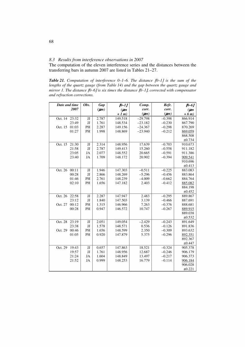
68

8.3 Results from interference observations in 2007

The computation of the eleven interference series and the distances between the transferring bars in autumn 2007 are listed in Tables 21–27.

Table 21. Computation of interference 0–1–6. The distance [0–1] is the sum of the

lengths of the quartz gauge (from Table 14) and the gap between the quartz gauge and

mirror 1. The distance [0–6] is six times the distance [0–1], corrected with compensator

and refraction corrections.

Date and time

2007

Obs. Gap

(µµµµm)

[[[[0–1]]]] (µµµµm

+ 1 m)

Comp.

corr.

(µµµµm)

Refr.

corr.

(µµµµm)

[[[[0–6]]]] (µµµµm

+ 6 m)

Oct. 14 23:32 JJ 2.787 149.518 –29.798 –0.398 866.914 23:49 JJ 1.761 148.534 –23.182 –0.230 867.790

Oct. 15 01:03 PH 2.287 149.156 –24.367 –0.298 870.269 01:27 PH 1.998 148.869 –23.940 –0.212 869.059

868.508 ±0.734

Oct. 15 21:30 JJ 2.314 148.956 17.639 –0.703 910.673 21:58 JJ 2.787 149.413 15.260 –0.558 911.182 23:05 JA 2.077 148.552 20.665 –0.591 911.386 23:40 JA 1.709 148.172 20.902 –0.394 909.541

910.696 ±0.413

Oct. 26 00:11 JJ 1.946 147.303 –0.511 –0.225 883.083 00:28 JJ 2.866 148.269 –5.296 –0.456 883.864 01:46 PH 2.761 148.239 –4.009 –0.662 884.764 02:10 PH 1.656 147.182 2.403 –0.412 885.082

884.198 ±0.452

Oct. 26 22:58 JJ 2.287 147.947 2.483 –0.295 889.867 23:12 JJ 1.840 147.503 3.139 –0.466 887.691

Oct. 27 00:12 PH 1.315 146.966 7.263 –0.376 888.681 00:28 PH 0.947 146.572 10.747 –0.267 889.915

889.038 ±0.532

Oct. 28 23:19 JJ 2.051 149.054 –2.429 –0.243 891.649 23:38 JJ 1.578 148.571 0.536 –0.126 891.836

Oct. 29 00:46 PH 1.656 148.599 2.350 –0.309 893.632 01:05 PH 0.920 147.879 5.375 –0.296 892.351

892.367 ±0.447

Oct. 29 19:43 JJ 0.657 147.863 18.521 –0.324 905.378 19:57 JJ 1.761 148.956 12.687 –0.246 906.179 21:24 JA 1.604 148.849 13.497 –0.217 906.373 21:52 JA 0.999 148.253 16.779 –0.114 906.184

906.028 ±0.221

69

Table 21 continued.

Date and time

2007

Obs. Gap

(µµµµm)

[[[[0–1]]]] (µµµµm

+ 1 m)

Comp.

corr.

(µµµµm)

Refr.

corr.

(µµµµm)

[[[[0–6]]]] (µµµµm

+ 6 m)

Nov. 6 20:53 JJ 1.972 145.879 –36.651 –0.168 838.453 21:25 JJ 2.761 146.756 –40.024 –0.134 840.378 22:53 PH 2.524 146.655 –38.809 –0.128 840.991 23:27 PH 3.865 148.056 –45.561 –0.250 842.526

840.587 ±0.843

Nov. 7 21:21 JJ 1.288 145.419 –31.835 –0.193 840.483 21:42 JJ 1.578 145.549 –32.529 –0.929 839.838 23:12 PH 2.182 146.070 –38.590 –0.364 837.466 23:38 PH 1.446 145.325 –33.535 –0.371 838.044

838.958 ±0.717

Nov. 8 19:08 JJ 3.339 147.723 –41.827 –0.225 844.287 19:29 JJ 1.394 145.849 –31.051 –0.192 843.851 20:54 PH 2.498 147.256 –36.544 –0.195 846.797 21:54 PH 1.315 146.231 –27.102 –0.136 850.146

846.270 ±1.446

Nov. 10 18:51 JJ 1.630 146.373 –20.902 –0.531 856.802 19:15 JJ 1.919 146.675 –21.220 –0.477 858.352 20:20 PH 1.078 145.863 –15.531 –0.249 859.397 20:52 PH 1.735 146.529 –20.196 –0.190 858.788

858.335 ±0.554

Nov. 11 21:55 JJ 2.603 146.830 –15.804 –1.005 864.173 22:20 JJ 3.023 147.301 –18.670 –1.199 863.934 23:40 PH 2.314 146.420 –13.815 –1.185 863.521

Nov. 12 00:12 PH 1.578 145.720 –9.597 –0.254 864.472 864.025 ±0.201

70

Table 22. Computation of interference 0–6–24. The distance [0–24] is four times the

distance [0–6] (from Table 21), corrected with compensator and refraction corrections.

Date and time

2007 4 × [[[[0–6]]]]

(µµµµm + 24 m)

Comp. corr.

(µµµµm)

Refr. corr.

(µµµµm)

[[[[0–24]]]] (µµµµm + 24 m)

Oct. 14 22:14 3 467.656 41.401 –0.745 3 508.312 Oct. 15 00:01 3 471.158 30.117 –1.171 3 500.104

00:23 3 481.075 30.149 0.287 3 511.511 01:40 3 476.237 21.194 –0.737 3 496.694

3 504.155 ±3.458

Oct. 15 20:57 3 642.693 –125.955 –0.874 3 515.864 22:10 3 644.728 –125.288 –1.860 3 517.580 22:25 3 645.545 –123.507 –1.821 3 520.217

Oct. 16 00:00 3 638.163 –120.916 –0.866 3 516.381 3 517.511 ±0.971

Oct. 25 23:26 3 532.333 –50.428 –1.307 3 480.598 Oct. 26 00:40 3 535.458 –51.996 –1.875 3 481.587

01:06 3 539.054 –52.295 –2.349 3 484.410 02:26 3 540.327 –56.319 –2.338 3 481.670

3 482.066 ±0.818

Oct. 26 22:34 3 559.468 –66.851 –0.520 3 492.097 23:24 3 550.762 –66.410 –1.220 3 483.132

Oct. 27 00:00 3 554.724 –66.900 –0.528 3 487.296 00:41 3 559.659 –66.166 –0.934 3 492.559

3 488.771 ±2.224

Oct. 28 22:53 3 566.597 –55.952 –0.420 3 510.225 23:52 3 567.345 –59.031 –0.720 3 507.594

Oct. 29 00:27 3 574.529 –60.831 –0.775 3 512.923 01:20 3 569.403 –59.904 –1.192 3 508.307

3 509.762 ±1.191

Oct. 29 19:18 3 621.512 –97.016 –0.866 3 523.630 20:07 3 624.715 –97.500 –0.541 3 526.674 20:37 3 625.492 –98.046 –1.090 3 526.356 22:08 3 624.735 –100.496 –1.445 3 522.794

3 524.863 ±0.971

Nov. 6 20:17 3 353.813 79.032 –1.037 3 431.808 21:35 3 361.512 80.873 –1.395 3 440.990 22:27 3 363.965 78.549 –1.121 3 441.393

Nov. 7 00:16 3 370.104 74.480 –1.226 3 443.358 3 439.387 ±2.579

71

Table 22 continued.

Date and time

2007 4 × [[[[0–6]]]]

(µµµµm + 24 m)

Comp. corr.

(µµµµm)

Refr. corr.

(µµµµm)

[[[[0–24]]]] (µµµµm + 24 m)

Nov. 7 20:45 3 361.933 105.626 –2.691 3 464.868 21:57 3 359.354 108.247 –2.992 3 464.609 22:49 3 349.864 115.730 –5.076 3 460.518 23:59 3 352.178 117.140 –1.570 3 467.748

3 464.436 ±1.487

Nov. 8 18:50 3 377.146 90.556 –0.657 3 467.045 19:39 3 375.403 87.108 –0.740 3 461.771 20:26 3 387.187 83.125 –0.596 3 469.716 22:14 3 400.582 71.089 –0.669 3 471.002

3 467.384 ±2.044

Nov. 10 18:25 3 427.209 35.884 –1.655 3 461.438 19:24 3 433.406 33.866 –1.699 3 465.573 20:01 3 437.589 32.930 –0.361 3 470.158 21:06 3 435.152 29.703 –0.615 3 464.240

3 465.352 ±1.819

Nov. 11 21:30 3 456.693 23.686 –0.631 3 479.748 22:31 3 455.737 23.517 –2.101 3 477.153 23:19 3 454.084 25.408 –1.814 3 477.678

Nov. 12 00:27 3 457.887 25.583 –3.267 3 480.203 3 478.695 ±0.752

72

Table 23. Computation of interference 0–24–72. The distance [0–72] is three times the

distance [0–24] (from Table 22), corrected with compensator and refraction corrections.

Date and time

2007 3 × [[[[0–24]]]]

(µµµµm + 72 m)

Comp. corr.

(µµµµm)

Refr. corr.

(µµµµm)

[[[[0–72]]]] (µµµµm + 72 m)

Oct. 14 22:01 10 512.466 34.004 2.559 10 549.029 Oct. 15 01:54 10 512.466 27.856 1.636 10 541.958

10 545.494 ±3.535

Oct. 15 20:46 10 552.532 –24.496 –3.043 10 524.993 Oct. 16 00:20 10 552.532 –17.518 2.076 10 537.090

10 531.042 ±6.049

Oct. 25 23:15 10 446.198 82.363 1.979 10 530.540 Oct. 26 02:39 10 446.198 80.329 –0.032 10 526.495

10 528.518 ±2.022

Oct. 26 22:24 10 466.314 64.161 2.283 10 532.758 Oct. 27 00:53 10 466.314 63.301 3.163 10 532.778

10 532.768 ±0.010

Oct. 28 22:37 10 529.286 31.461 1.852 10 562.599 Oct. 29 01:34 10 529.286 26.168 1.637 10 557.091

10 559.845 ±2.754

Oct. 29 19:08 10 574.590 –2.285 0.476 10 572.781 22:29 10 574.590 –0.363 0.391 10 574.618

10 573.700 ±0.918

Nov. 6 19:56 10 318.161 146.574 0.953 10 465.688 Nov. 7 00:20 10 318.161 146.286 1.262 10 465.709

10 465.699 ±0.011

Nov. 7 20:33 10 393.307 91.769 2.910 10 487.986 Nov. 8 00:11 10 393.307 103.858 1.576 10 498.741

10 493.363 ±5.377

Nov. 8 18:40 10 402.151 100.403 0.363 10 502.917 20:26 10 402.151 87.549 1.870 10 491.570

10 497.243 ±5.674

Nov. 10 18:15 10 396.057 108.904 0.485 10 505.446 21:17 10 396.057 107.235 2.118 10 505.410

10 505.428 ±0.018

Nov. 11 21:17 10 436.086 49.404 1.297 10 486.787 Nov. 12 00:39 10 436.086 50.124 1.506 10 487.716

10 487.252 ±0.464

73

Table 24. Computation of interference 0–72–216. The distance [0–216] is three times the

distance [0–72] (from Table 23), corrected with compensator and refraction corrections.

Date and time

2007 3 × [[[[0–72]]]]

(µµµµm + 216 m)

Comp. corr.

(µµµµm)

Refr. corr.

(µµµµm)

[[[[0–216]]]] (µµµµm + 216 m)

Oct. 14 21:42 31 636.481 41.656 –6.444 31 671.693 Oct. 15 02:14 31 636.481 41.118 –13.321 31 664.278

31 667.986 ±3.708

Oct. 15 20:22 31 593.126 –10.668 –10.863 31 571.595 Oct. 16 00:38 31 593.126 –18.521 –1.727 31 572.878

31 572.236 ±0.642

Oct. 25 22:58 31 585.553 –60.668 0.288 31 525.173 Oct. 26 02:57 31 585.553 –55.413 –11.951 31 518.189

31 521.681 ±3.492

Oct. 26 22:09 31 598.303 –33.993 0.176 31 564.486 Oct. 27 01:12 31 598.303 –42.591 2.119 31 557.831

31 561.158 ±3.328

Oct. 28 22:19 31 679.536 –80.139 –7.991 31 591.406 Oct. 29 01:55 31 679.536 –76.251 –15.283 31 588.002

31 589.704 ±1.702

Oct. 29 18:55 31 721.100 –88.501 –11.644 31 620.955 22:55 31 721.100 –77.427 –20.537 31 623.136

31 622.045 ±1.091

Nov. 6 19:36 31 397.097 51.959 –4.027 31 445.029 Nov. 7 00:48 31 397.097 60.096 –4.949 31 452.244

31 448.636 ±3.608

Nov. 7 20:13 31 480.090 –17.639 –6.055 31 456.396 Nov. 8 00:31 31 480.090 –15.036 –6.301 31 458.753

31 457.574 ±1.178

Nov. 8 18:26 31 491.729 –9.004 2.017 31 484.742 22:43 31 491.729 –12.589 –8.277 31 470.863

31 477.803 ±6.940

Nov. 10 17:58 31 516.283 –21.929 –1.485 31 492.869 21:31 31 516.283 –22.541 –0.233 31 493.509

31 493.189 ±0.320

Nov. 11 21:00 31 461.755 22.884 –6.556 31 478.083 Nov. 12 00:55 31 461.755 18.225 –6.810 31 473.170

31 475.626 ±2.457

74

Table 25. Computation of interference 0–216–432. The distance [0–432] is two times the

distance [0–216] (from Table 24), corrected with compensator and refraction

corrections.

Date and time

2007 2 × [[[[0–216]]]]

(µµµµm + 432 m)

Comp. corr.

(µµµµm)

Refr. corr.

(µµµµm)

[[[[0–432]]]] (µµµµm + 432 m)

Oct. 14 21:14 63 335.972 50.439 –9.026 63 377.385 Oct. 15 02:37 63 335.972 59.306 –13.611 63 381.667

63 379.526 ±2.141

Oct. 15 19:55 63 144.473 33.576 –22.031 63 156.018 Oct. 16 01:12 63 144.473 11.445 2.287 63 158.205

63 157.111 ±1.093

Oct. 25 22:37 63 043.362 65.368 –3.408 63 105.322 Oct. 26 03:32 63 043.362 80.982 –25.539 63 098.805

63 102.063 ±3.258

Oct. 26 21:08 63 122.316 30.453 –10.232 63 142.537 Oct. 27 01:53 63 122.316 28.001 –5.287 63 145.030

63 143.784 ±1.247

Oct. 28 21:54 63 179.408 32.194 –11.983 63 199.619 Oct. 29 02:21 63 179.408 33.855 –17.271 63 195.992

63 197.806 ±1.814

Oct. 29 18:26 63 244.091 –6.435 –23.623 63 214.033 23:44 63 244.091 9.878 –31.253 63 222.716

63 218.374 ±4.341

Nov. 6 19:11 62 897.273 85.276 –5.711 62 976.838 Nov. 7 01:12 62 897.273 96.956 –5.817 62 988.412

62 982.625 ±5.787

Nov. 7 19:43 62 915.149 119.071 –6.357 63 027.863 Nov. 8 18:05 62 955.606 126.660 –1.612 63 080.654

23:05 62 955.606 125.604 –0.020 63 081.190 63 080.922 ±0.268

Nov. 10 17:36 62 986.378 99.734 –8.221 63 077.891 21:58 62 986.378 91.566 –10.014 63 067.930

63 072.911 ±4.981

Nov. 11 18:57 62 951.252 95.410 –5.823 63 040.839 Nov. 12 01:16 62 951.252 95.552 –11.511 63 035.293

63 038.066 ±2.773

75

Table 26. Computation of interference 0–432–864. The distance [0–864] is two times the

distance [0–432] (from Table 25), corrected with compensator and refraction

corrections.

Date and time

2007 2 × [[[[0–432]]]]

(µµµµm + 864 m)

Comp. corr.

(µµµµm)

Refr. corr.

(µµµµm)

[[[[0–864]]]] (µµµµm + 864 m)

Oct. 26 21:08 126 287.567 80.207 31.731 126 399.505 Oct. 27 03:58 126 287.567 132.984 –8.374 126 412.177

126 405.841 ±6.336

Oct. 28 21:08 126 395.612 45.204 14.560 126 455.376 Oct. 29 03:07 126 395.612 42.141 –4.815 126 432.938

126 444.157 ±11.219

Oct. 29 17:35 126 436.749 22.354 33.982 126 493.085 Oct. 30 00:56 126 436.749 –4.758 46.327 126 478.318

126 485.701 ±7.384

Nov. 6 18:21 125 965.249 73.473 8.144 126 046.866 Nov. 7 18:40 126 055.726 107.849 –13.775 126 149.800 Nov. 8 17:30 126 161.844 80.442 1.661 126 243.947

23:40 126 161.844 74.214 3.841 126 239.899 126 241.923 ±2.024

Nov. 10 17:01 126 145.822 68.132 11.131 126 225.085 Nov. 11 18:16 126 076.133 98.077 –10.719 126 163.491 Nov. 12 01:48 126 076.133 78.992 –2.386 126 152.739

126 158.115 ±5.376

76

Table 27. Distances between transferring bars (mm) in 2007, using equal weights. For

the interference observations I (from Tables 21–26) the difference of transfer readings L

and the thickness of mirror 0, D0 = 19.985 mm, are added: Bν = Iν –Lν +L0 +D0. uB is the

experimental standard deviation of the mean ��.

2007 I6 L6 L0 B6 I24 L24 L0 B24

14–15 X 0.8685 20.0390 11.4225 12.237 3.5042 14.3145 11.4225 20.597 15–16 X 0.9107 20.0640 11.4285 12.260 3.5175 14.3305 11.4285 20.601 25–26 X 0.8842 20.0680 11.4265 12.228 3.4821 14.3385 11.4265 20.555 26–27 X 0.8890 20.0645 11.4270 12.237 3.4888 14.3390 11.4270 20.562 28–29 X 0.8924 20.0300 11.4210 12.268 3.5098 14.3270 11.4210 20.589 29–30 X 0.9060 20.0395 11.4220 12.274 3.5249 14.3395 11.4220 20.592

6–7 XI 0.8406 20.0505 11.4275 12.203 3.4394 14.3360 11.4275 20.516 7 XI 0.8390 20.0405 11.4285 12.212 3.4644 14.3530 11.4285 20.525 8 XI 0.8463 20.0435 11.4245 12.212 3.4674 14.3505 11.4245 20.526

10 XI 0.8583 20.0480 11.4245 12.220 3.4654 14.3470 11.4245 20.528 11–12 XI 0.8640 20.0595 11.4260 12.216 3.4787 14.3640 11.4260 20.526 �� 12.233 20.556

uB ±0.007 ±0.010 2007 I72 L72 L0 B72 I216 L216 L0 B216

14–15 X 10.5455 21.9840 11.4225 19.969 31.6680 11.0995 11.4225 51.976 15–16 X 10.5310 21.9990 11.4285 19.946 31.5722 11.1005 11.4285 51.885 25–26 X 10.5285 22.0355 11.4265 19.905 31.5217 11.0875 11.4265 51.846 26–27 X 10.5328 22.0285 11.4270 19.916 31.5612 11.1025 11.4270 51.871 28–29 X 10.5598 22.0275 11.4210 19.938 31.5897 11.0885 11.4210 51.907 29–30 X 10.5737 22.0380 11.4220 19.943 31.6220 11.1105 11.4220 51.919

6–7 XI 10.4657 22.0115 11.4275 19.867 31.4486 11.0810 11.4275 51.780 7 XI 10.4934 22.0305 11.4285 19.876 31.4576 11.0650 11.4285 51.806 8 XI 10.4972 22.0245 11.4245 19.882 31.4778 11.0600 11.4245 51.827

10 XI 10.5054 22.0325 11.4245 19.882 31.4932 11.0700 11.4245 51.833 11–12 XI 10.4873 22.0175 11.4260 19.881 31.4756 11.0715 11.4260 51.815 �� 19.910 51.860

uB ±0.010 ±0.017 2007 I432 L432 L0 B432 I864 L864 L0 B864

14–15 X 63.3795 14.8625 11.4225 79.925 – – – – 15–16 X 63.1571 14.8595 11.4285 79.711 – – – – 25–26 X 63.1021 14.8625 11.4265 79.651 – – – – 26–27 X 63.1438 14.8595 11.4270 79.696 126.4058 12.3285 11.4270 145.489 28–29 X 63.1978 14.8585 11.4210 79.745 126.4442 12.2985 11.4210 145.552 29–30 X 63.2184 14.8615 11.4220 79.764 126.4857 12.3020 11.4220 145.591

6–7 XI 62.9826 14.8625 11.4275 79.533 126.0469 12.3020 11.4275 * 145.157 7 XI 63.0279 14.8635 11.4285 * 79.578 126.1498 12.3050 11.4285 * 145.258 8 XI 63.0809 14.8600 11.4245 79.630 126.2419 12.3025 11.4245 145.349

10 XI 63.0729 14.8630 11.4245 79.619 126.2251 12.3020 11.4245 * 145.333 11–12 XI 63.0381 14.8600 11.4260 79.589 126.1581 12.2980 11.4260 145.271 �� 79.681 145.404

uB ±0.034 ±0.053 * with ½-weight

77

8.4 Final lengths

The distances between the transferring bars are corrected to the final lengths between the underground markers, as shown in Tables 28 and 29.

Table 28. Computation of baseline length in 2005.

0–24

24 m +

(mm)

0–72

72 m +

(mm)

0–216

216 m +

(mm)

0–432

432 m +

(mm)

Distance between transferring bars

(Table 20) 24.000 20.032 54.704 78.081

Projection correction (Table 11) +9.591 –4.191 +1.052 +22.310

Correction to the level of

underground marker 0 (Table 9)

–0.286

–0.853

–2.538

–4.998

Mirror coating correction

(Section 7.3) –0.000 –0.001 –0.002 –0.005

Mirror body correction

(Section 7.3) –0.071 –0.002 –0.010 –0.013

Air-pressure difference correction

(Section 7.4)

–0.000

–0.000

–0.004

–0.016

Nonparallelism correction

(Table 10) +0.000 +0.000 +0.001 +0.001

Final length 33.234 14.985 53.203 95.360

Table 29. Computation of baseline length in 2007.

0–24

24 m +

(mm)

0–72

72 m +

(mm)

0–216

216 m +

(mm)

0–432

432 m +

(mm)

0–864

864 m +

(mm)

Distance between transferring

bars (Table 27) 20.556 19.910 51.860 79.681 145.404

Projection correction (Table 12) +13.014 –4.109 +3.821 +20.638 –12.745

Correction to the level of

underground marker 0 (Table 9)

–0.281

–0.848

–2.538

–5.003

–9.725

Mirror coating correction

(Section 7.3)

–0.000

–0.001

–0.002

–0.005

–0.010

Mirror body correction

(Section 7.3)

–0.071

–0.002

–0.010

–0.013

–0.001

Air-pressure difference correction

(Section 7.4)

–0.000

–0.000

–0.004

–0.016

–0.062

Nonparallelism correction

(Table 10)

+0.000

+0.000

+0.001

+0.001

+0.003

Final length 33.218 14.950 53.128 95.283 122.864

78

9 Estimation of uncertainty of measurement

9.1 Combined uncertainty of the lengths between the underground markers

Since the principle of the Väisälä interference measurement method is essentially simple and straightforward, the list of components of uncertainty of measurement remains rather short. In practice, the performance is extremely laborious because measurements in unfavourable conditions are not possible at all. This self-protective mechanism is the main reason why the results and uncertainties are not practically affected by the measurement conditions (if a measurement succeeds). An evaluation of the combined uncertainty of the measurement for the lengths between the underground markers is presented in Tables 30 and 31.

The evaluation of standard uncertainty due to interference observations, transfer readings and projection measurements is based on statistical analysis, and experimental standard deviations of the means are used (Type A, according to GUM, BIPM 2008b). An evaluation of the other components (Type B) is based on calibration results for the absolute length of the quartz gauge and on previous knowledge of the thicknesses of the mirror coatings and on experience with the thermal behaviour of the quartz gauge.

For the absolute length of the quartz gauge, the estimated standard uncertainty ±35 nm is reasonable, based on the latest absolute calibrations and frequent comparisons. The estimate of uncertainty due to the temperature of the quartz gauge, ±20 nm/m, is equivalent to the determination of the temperature with ±0.05° standard uncertainty, which seems realistic. Tables 13 and 14 show that (with a few exceptions) the observed temperature t changes during one half-set with the quartz gauge in two positions, 0.1° or less. The estimate of uncertainty is valid only if the quartz gauge is properly stored and handled before and during the measurement.

Some dependence on temperature can be found both in the distances between the mirrors and between the transferring bars, especially for the shortest distances in both 2005 and 2007. The mechanism causing this is not clear. Most of this variation seems not to multiply. The variation is of the order of about 0.01 mm/°. The variation is at the same tens of micrometres level as what is often present in the projection measurements at 0. It is not possible to perform interference measurements in warm temperatures in order to examine the variation more thoroughly, but most calibrations utilizing the baseline are also performed in circumstances close to those which prevail during the interference measurements.

The different thicknesses of mirror coatings at mirrors 0 and 1 are difficult to determine, since the mirror surfaces are not perfectly flat. Therefore, the estimated standard uncertainty must be kept quite large. There is no reason to change the values that were determined for the measurements in Chengdu, China in 1998 (Jokela et al. 2000). The estimated standard uncertainty was first ±20 nm/m, but for the measurements in Gödöllı, Hungary in 1999 (Jokela et al.

79

2001) and later in Nummela it was doubled to ±40 nm/m. There have been no noteworthy changes (e.g., due to scuffing) in the mirrors and their coatings since 1998. The estimated standard uncertainty was increased just to be on the safe side, since the much smaller uncertainty that was previously achieved in the determinations of the thicknesses of mirror coatings has not been achieved in the latest determinations. Improving the method for determining the thickness of mirror coatings is one of the first challenges in decreasing the combined measurement uncertainty.

Table 30. Evaluation of the combined uncertainty of measurement in 2005 (µm).

0–24 0–72 0–216 0–432

Uncertainty uB due to interference observations and transfer readings 9 9 15 22

Uncertainty uP due to projection measurements 34 43 38 35

Uncertainty due to the absolute length of the quartz gauge 1 3 8 15

Uncertainty due to the temperature of the quartz gauge 0 1 4 9

Uncertainty due to the thicknesses of mirror coatings 1 3 9 17

Uncertainty due to the levellings 0 1 2 2

Combined standard uncertainty uc 35 44 43 48

Combined expanded uncertainty U=2uc 70 88 86 96

Table 31. Evaluation of the combined uncertainty of measurement in 2007 (µm).

0–24 0–72 0–216 0–432 0–864

Uncertainty uB due to interference observations and transfer readings 10 10 17 34 53

Uncertainty uP due to projection measurements 33 19 18 16 18

Uncertainty due to the absolute length of the quartz gauge 1 3 8 15 30

Uncertainty due to the temperature of the quartz gauge 0 1 4 9 17

Uncertainty due to the thicknesses of mirror coatings 1 3 9 17 34

Uncertainty due to the levellings 0 1 2 2 4

Combined standard uncertainty uc 34 22 28 45 74

Combined expanded uncertainty U=2uc 69 45 55 89 149

80

The uncertainty due to precise levellings is related to the geometrical reductions and evaluated on the grounds of the levelling results. This includes both levelling along the baseline and the levelling of instruments on the observation pillars. Smaller than 1 mm uncertainties in the levelled heights are fairly easy to obtain with calibrated instruments, which keeps the uncertainty of geometrical reductions at a micrometre level.

The combined standard uncertainty in Tables 30 and 31 has been computed according to GUM Sections 5 and 6 (BIPM 2008b) from the standard uncertainties of listed components. The combined expanded uncertainty is the combined standard uncertainty multiplied by the coverage factor k = 2.

9.2 Some supplementary analysis of uncertainty of measurement

In estimating the uncertainty of interference measurements, it has been customary to compute two uncertainty estimates. In addition to the one previously presented for the distances between the transferring bars, uB, another one for the distances between the mirror surfaces, uM, can be computed and compared to it. The former should theoretically be larger than the latter, since it includes the possible movements of observation pillars during the several weeks or months of measurements. It also includes the (very small) uncertainty of the transfer readings. Only the former is used in the final computation of combined uncertainty, whereas the latter is computed just for scrutiny. The computation method applied here is identical and thus comparable with the computations in the several previous publications on interference measurements.

In Tables 32 and 33, uncertainties uI for every interference observation stage (I = 72, 216, 432 or 864) are derived from experimental standard deviations of the means uI,i (from Tables 15–19 and 21–26) and number of observation nights ns with the formula �� � ��∑��,� � !⁄ .

Half nights in 2007 mean half (one-way) measurements, and nobs is the number of observations in one night. The combined uncertainties uI

acc are obtained from the uncertainties uI by using the formulas for the standard deviations of products and sums; in 2005:

0–72: #$�3 & 1.34� � �3.18� µm = 5 µm, 0–216: # $�9 & 1.34� � �3 & 3.18� � �6.53� µm = 17 µm, 0–432: # $�18 & 1.34� � �6 & 3.18� � �2 & 6.53� � �4.71� µm = 34 µm,

and in 2007: 0–72: # $�3 & 1.85� � �3.34� µm = 6 µm, 0–216: # $�9 & 1.85� � �3 & 3.34� � �3.17� µm = 20 µm, 0–432: # $�18 & 1.85� � �6 & 3.34� � �2 & 3.17� � �3.26� µm = 40 µm, 0–864: # $�36 & 1.85� � �12 & 3.34� � �4 & 3.17� � �2 & 3.26� � �7.12� µm = 79 µm.

81

In these combined uncertainties, the value u24 for 0–24, 1.34 µm in 2005 and 1.85 µm in 2007 is treated differently from the other values, since it includes a set of random errors, which do not affect the longer distances. These random errors are mostly related to working with the quartz gauge.

From the combined uncertainties uIacc in one observation series, the

uncertainties uM for the distances between the mirror surfaces after the entire measurement are estimated by dividing uI

acc by $ ! (Tables 32 and 33). The uncertainties uB for the distances between the transferring bars are computed in Tables 20 and 27 and used in the evaluation of combined uncertainty in Tables 30 and 31. As expected, for all distances uM are smaller than uB.

Table 32. Comparison of the standard uncertainties of the distances between the mirror

surfaces (uM) or between the transferring bars (uB) in 2005.

0–24 0–72 0–216 0–432 ns 7 7 7 7

nobs 4 2 2 2 uI (µm) ±1 ±3 ±7 ±5

uIacc (µm) ±1 ±5 ±17 ±34

uM (µm) ±0 ±2 ±6 ±13 uB (µm) ±9 ±9 ±15 ±22

Table 33. Comparison of the standard uncertainties of the distances between the mirror

surfaces (uM) or between the transferring bars (uB) in 2007.

0–24 0–72 0–216 0–432 0–864 ns 11 11 11 10 + ½ 5 + 3×½

nobs 4 2 2 2 (1) 2 (1) uI (µm) ±2 ±3 ±3 ±3 ±7

uIacc (µm) ±2 ±6 ±20 ±40 ±79

uM (µm) ±1 ±2 ±6 ±12 ±31 uB (µm) ±10 ±10 ±17 ±34 ±53

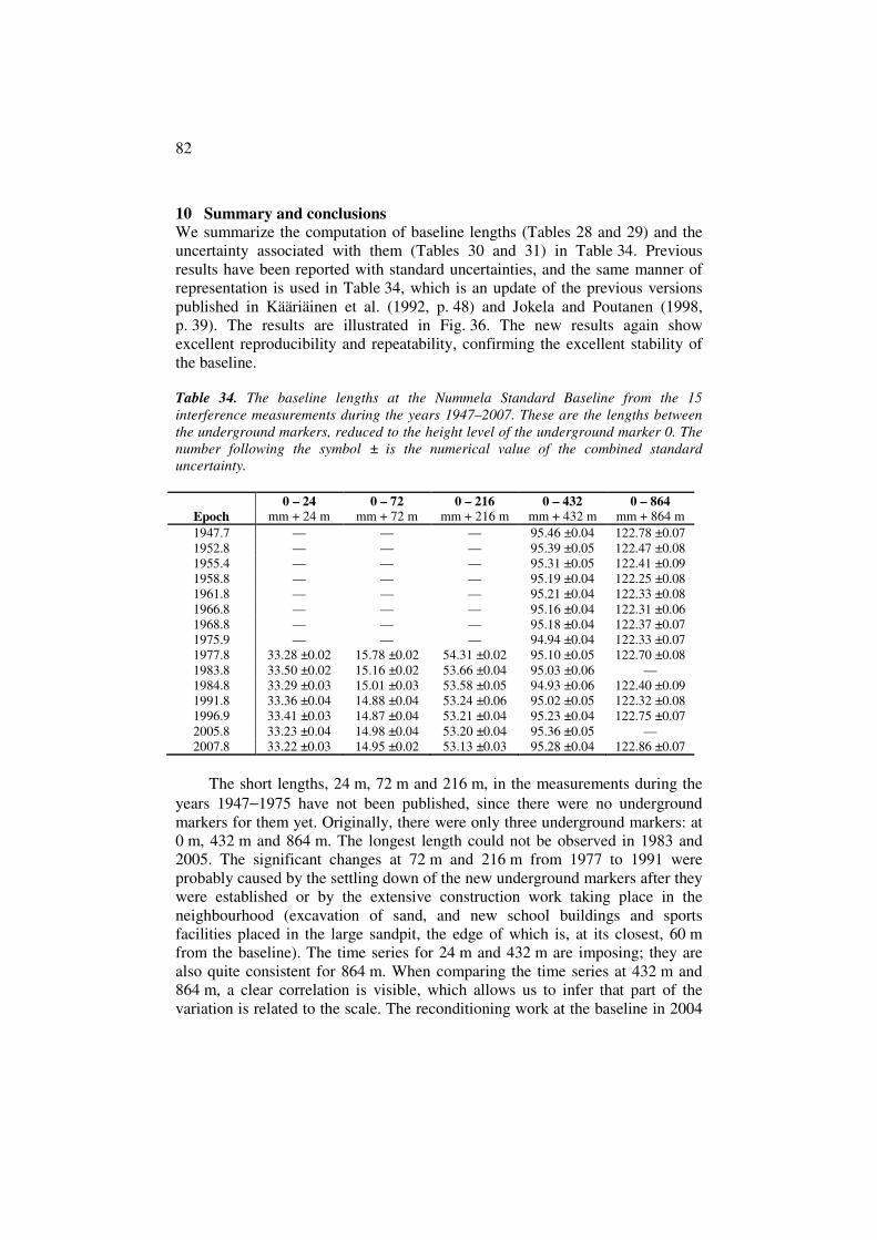
82

10 Summary and conclusions

We summarize the computation of baseline lengths (Tables 28 and 29) and the uncertainty associated with them (Tables 30 and 31) in Table 34. Previous results have been reported with standard uncertainties, and the same manner of representation is used in Table 34, which is an update of the previous versions published in Kääriäinen et al. (1992, p. 48) and Jokela and Poutanen (1998, p. 39). The results are illustrated in Fig. 36. The new results again show excellent reproducibility and repeatability, confirming the excellent stability of the baseline.

Table 34. The baseline lengths at the Nummela Standard Baseline from the 15

interference measurements during the years 1947–2007. These are the lengths between

the underground markers, reduced to the height level of the underground marker 0. The

number following the symbol ± is the numerical value of the combined standard

uncertainty.

0 – 24 0 – 72 0 – 216 0 – 432 0 – 864

Epoch mm + 24 m mm + 72 m mm + 216 m mm + 432 m mm + 864 m 1947.7 — — — 95.46 ±0.04 122.78 ±0.07 1952.8 — — — 95.39 ±0.05 122.47 ±0.08 1955.4 — — — 95.31 ±0.05 122.41 ±0.09 1958.8 — — — 95.19 ±0.04 122.25 ±0.08 1961.8 — — — 95.21 ±0.04 122.33 ±0.08 1966.8 — — — 95.16 ±0.04 122.31 ±0.06 1968.8 — — — 95.18 ±0.04 122.37 ±0.07 1975.9 — — — 94.94 ±0.04 122.33 ±0.07 1977.8 33.28 ±0.02 15.78 ±0.02 54.31 ±0.02 95.10 ±0.05 122.70 ±0.08 1983.8 33.50 ±0.02 15.16 ±0.02 53.66 ±0.04 95.03 ±0.06 — 1984.8 33.29 ±0.03 15.01 ±0.03 53.58 ±0.05 94.93 ±0.06 122.40 ±0.09 1991.8 33.36 ±0.04 14.88 ±0.04 53.24 ±0.06 95.02 ±0.05 122.32 ±0.08 1996.9 33.41 ±0.03 14.87 ±0.04 53.21 ±0.04 95.23 ±0.04 122.75 ±0.07 2005.8 33.23 ±0.04 14.98 ±0.04 53.20 ±0.04 95.36 ±0.05 — 2007.8 33.22 ±0.03 14.95 ±0.02 53.13 ±0.03 95.28 ±0.04 122.86 ±0.07

The short lengths, 24 m, 72 m and 216 m, in the measurements during the

years 1947−1975 have not been published, since there were no underground markers for them yet. Originally, there were only three underground markers: at 0 m, 432 m and 864 m. The longest length could not be observed in 1983 and 2005. The significant changes at 72 m and 216 m from 1977 to 1991 were probably caused by the settling down of the new underground markers after they were established or by the extensive construction work taking place in the neighbourhood (excavation of sand, and new school buildings and sports facilities placed in the large sandpit, the edge of which is, at its closest, 60 m from the baseline). The time series for 24 m and 432 m are imposing; they are also quite consistent for 864 m. When comparing the time series at 432 m and 864 m, a clear correlation is visible, which allows us to infer that part of the variation is related to the scale. The reconditioning work at the baseline in 2004

83

and 2007 seems to have been successful and did not disturb it, since all of the changes from 1996 to 2005 and 2007 are smaller than 0.2 mm.

Depending on the present and future activities at the baseline, the next re-measurement with interference measurements, supported with new absolute calibrations and comparisons of the quartz gauges, is necessary within the next 5–10 years. New innovations in absolute long-distance measurements are being developed, and the new results from interference measurements at the Nummela Standard Baseline can be used for validating or comparing new methods or instruments. So far, the Nummela Standard Baseline still remains the most accurate measurement standard for length measurements in field conditions.

Fig. 36. The results of the 15 interference measurements of the Nummela Standard

Baseline during the years 1947–2007.

32,5

33,0

33,5

34,0

1940 1960 1980 2000 2020

mm

+ 2

4 m

14,5

15,0

15,5

16,0

1940 1960 1980 2000 2020

mm

+ 7

2 m

53,0

53,5

54,0

54,5

1940 1960 1980 2000 2020

mm

+ 2

16

m

94,5

95,0

95,5

96,0

1940 1960 1980 2000 2020

mm

+ 4

32

m

122,0

122,5

123,0

123,5

1940 1960 1980 2000 2020

mm

+ 8

64

m

84

References

BIPM (2008a). International vocabulary of metrology – Basic and general concepts and associated terms (VIM). JCGM 200:2008. Joint Committee for Guides in Metrology. http://www.bipm.org/ BIPM (2008b). Evaluation of measurement data – Guide to the expression of uncertainty in measurement. JGCM 100:2008. Joint Committee for Guides in Metrology. http://www.bipm.org/ Honkasalo, T. (1950). Measuring of the 864 m-long Nummela standard base line with the Väisälä light interference comparator and some investigations into invar wires. Publ. Finn. Geod. Inst. no. 37. 88 pages. Jokela, J. (1994). The 1993 adjustment of the Finnish First-Order Terrestrial Triangulation. Publ. Finn. Geod. Inst. no. 119. 137 pages. Jokela, J., P. Häkli, J. Ahola, A. Būga and R. Putrimas (2009). On traceability of long distances. Proceedings of the XIX IMEKO World Congress Fundamental and Applied Metrology, Lisbon, Portugal, September 6–11, 2009, pp. 1882–1887, http://www.imeko2009.it.pt/Papers/FP_100.pdf (cited July 9th, 2010). Jokela, J., P. Häkli, R. Kugler, H. Skorpil, M. Matus and M Poutanen (2010). Calibration of the BEV Geodetic Baseline. Proceedings of the XXIV FIG International Congress 2010 ”Facing the Challenges – Building the Capacity”, Sydney, Australia, April 11–16, 2010. Available at FIG Surveyors Reference Library, http://www.fig.net/srl/ (cited July 9th, 2010), 15 p. Jokela, J. and M. Poutanen (1998). The Väisälä baselines in Finland. Publ. Finn. Geod. Inst. no. 127. 61 pages. Jokela, J., M. Poutanen, Zs. Németh and G. Virág (2001). Remeasurement of the Gödöllı Standard Baseline. Publ. Finn. Geod. Inst. no. 131. 37 pages. Jokela, J., M. Poutanen, J.Z. Zhao, W.L. Pei, Z.Y. Hu and S.S. Zhang (2000). The Chengdu Standard Baseline. Publ. Finn. Geod. Inst. no. 130. 46 pages. Kääriäinen, J. (1984). Baseline measurements with invar wires in Finland in 1958–1970. Publ. Finn. Geod. Inst. no. 100. 74 pages. Kääriäinen, J., R. Konttinen and M. Poutanen (1992). Interference measurements of the Nummela Standard Baseline in 1977, 1983, 1984 and 1991. Publ. Finn. Geod. Inst. no. 114. 78 pages.

85

Kiviniemi, A. (1970). Niinisalo calibration baseline. Publ. Finn. Geod. Inst. no. 69. 36 pages. Konttinen, R. (1994). Observation results. Geodimeter observations in 1971–72, 1974–80 and 1984–85. Publ. Finn. Geod. Inst. no. 117. 58 pages. Kukkamäki, T.J. (1933). Untersuchungen über die Meterendmasse aus geschmolzenem Quartz nach lichinterferometrischen Methoden. Uuden Auran osakeyhtiön kirjapaino, Turku. 83 pages. Kukkamäki, T.J. (1969). Ohio Standard Baseline. Annales Academiae Scientiarum Fennicae. Series A. III. 102. Suomalainen tiedeakatemia, Helsinki. 59 pages. Kukkamäki, T.J. (1978). Väisälä interference comparator. Publ. Finn. Geod. Inst. no. 87. 49 pages. Lassila, A., J. Jokela, M. Poutanen and J. Xu (2003). Absolute calibration of quartz bars of Väisälä interferometer by white light gauge block interferometer. Proc. XVII IMEKO World Congress, June 22-27, 2003, Dubrovnik, Croatia, p. 1886-1890. MIKES (2000). Certificates of Calibration, no. M-L 74, M-L 75, M-L 76, M-L 78. Niemi, A. (2001). Metrin vertaus. Manuscript for a manual for comparisons of quartz metres at Tuorla. Niemi, A. (2005). Metrikomparaattorin käyttö. Manuscript for a manual for the comparator of quartz metres at Tuorla. Parm, T. (1976). High precision traverse of Finland. Publ. Finn. Geod. Inst. no. 79. 108 pages. PTB (1996). Calibration certificate, Ref. No. 4.31-23912/95. Väisälä, Y. (1923). Die Anwendung der Lichtinterferenz zu Längenmessungen auf grösseren Distanzen. Publ. Finn. Geod. Inst., Nr 2. Väisälä, Y. and L. Oterma (1967). System of Quartzmetres and the Absolute Length of its Gauges. Metrologia, Vol. 3, No. 2, p. 37–41.

Suomen Geodeettisen laitoksen julkaisut:

Veröffentlichungen des Finnischen Geodätischen Institutes:

Publications of the Finnish Geodetic Institute:

1. Y. VÄISÄLÄ: Tafeln für geodätische Berechnungen nach den Erddimensionen von Hayford. Helsinki 1923. 30 S.

2. Y. VÄISÄLÄ: Die Anwendung der Lichtinterferenz zu Längenmessungen auf grösseren Distanzen. Helsinki 1923. 22 S.

3. ILMARI BONSDORFF, Y. LEINBERG, W. HEISKANEN: Die Beobachtungsergebnisse der südfinnischen Triangulation in den Jahren 1920-1923. Helsinki 1924. 235 S.

4. W. HEISKANEN: Untersuchungen über Schwerkraft und Isostasie. Helsinki 1924. 96 S. 1 Karte. 5. W. HEISKANEN: Schwerkraft und isostatische Kompensation in Norwegen. Helsinki 1926. 33 S. 1 Karte. 6. W. HEISKANEN: Die Erddimensionen nach den europäischen Gradmessungen. Helsinki 1926. 26 S. 7. ILMARI BONSDORFF, V.R. ÖLANDER, Y. LEINBERG: Die Beobachtungsergebnisse der südfinnischen

Triangulation in den Jahren 1924-1926. Helsinki 1927. 164 S. 1 Karte. 8. V.R. ÖLANDER: Ausgleichung einer Dreieckskette mit Laplaceschen Punkten. Helsinki 1927. 49 S. 1 Karte. 9. U. PESONEN: Relative Bestimmungen der Schwerkraft auf den Dreieckspunkten der südfinnischen

Triangulation in den Jahren 1924-1925. Helsinki 1927. 129 S. 10. ILMARI BONSDORFF: Das Theorem von Clairaut und die Massenverteilung im Erdinnern. Helsinki 1929.

10 S. 11. ILMARI BONSDORFF, V.R. ÖLANDER, W. HEISKANEN, U. PESONEN: Die Beobachtungsergebnisse der

Triangulationen in den Jahren 1926-1928. Helsinki 1929. 139 S. 1 Karte. 12. W. HEISKANEN: Über die Elliptizität des Erdäquators. Helsinki 1929. 18 S. 13. U. PESONEN: Relative Bestimmungen der Schwerkraft in Finnland in den Jahren 1926-1929. Helsinki 1930.

168 S. 1 Karte. 14. Y. VÄISÄLÄ: Anwendung der Lichtinterferenz bei Basismessungen. Helsinki 1930. 47 S. 15. M. FRANSSILA: Der Einfluss der den Pendel umgebenden Luft auf die Schwingungszeit beim

v. Sterneckschen Pendelapparat. Helsinki 1931. 23 S. 16. Y. LEINBERG: Ergebnisse der astronomischen Ortsbestimmungen auf den finnischen Dreieckspunkten.

Helsinki 1931. 162 S. 17. V.R. ÖLANDER: Über die Beziehung zwischen Lotabweichungen und Schwereanomalien sowie über das

Lotabweichungssystem in Süd-Finnland. Helsinki 1931. 23 S. 18. PENTTI KALAJA, UUNO PESONEN, V.R. ÖLANDER, Y. LEINBERG: Beobachtungsergebnisse. Helsinki 1933.

240 S. 1 Karte. 19. R.A. HIRVONEN: The continental undulations of the geoid. Helsinki 1934. 89 pages. 1 map. 20. ILMARI BONSDORFF: Die Länge der Versuchsbasis von Helsinki und Längenveränderungen der Invardrähte

634-637. Helsinki 1934. 41 S. 21. V.R. ÖLANDER: Zwei Ausgleichungen des grossen südfinnischen Dreieckskranzes. Helsinki 1935. 66 S.

1 Karte. 22. U. PESONEN, V.R. ÖLANDER: Beobachtungsergebnisse. Winkelmessungen in den Jahren 1932-1935. Helsinki

1936. 148 S. 1 Karte. 23. R.A. HIRVONEN: Relative Bestimmungen der Schwerkraft in Finnland in den Jahren 1931, 1933 und 1935.

Helsinki 1937. 151 S. 24. R.A. HIRVONEN: Bestimmung des Schwereunterschiedes Helsinki-Potsdam im Jahre 1935 und Katalog der

finnischen Schwerestationen. Helsinki 1937. 36 S. 1 Karte. 25. T.J. KUKKAMÄKI: Über die nivellitische Refraktion. Helsinki 1938. 48 S. 26. Finnisches Geodätisches Institut 1918-1938. Helsinki 1939. 126 S. 2 Karten. 27. T.J. KUKKAMÄKI: Formeln und Tabellen zur Berechnung der nivellitischen Refraktion. Helsinki 1939. 18 S. 28. T.J. KUKKAMÄKI: Verbesserung der horizontalen Winkelmessungen wegen der Seitenrefraktion. Helsinki

1939. 18 S. 29. ILMARI BONSDORFF: Ergebnisse der astronomischen Ortsbestimmungen im Jahre 1933. Helsinki 1939. 47 S. 30. T. HONKASALO: Relative Bestimmungen der Schwerkraft in Finnland im Jahre 1937. Helsinki 1941. 78 S. 31. PENTTI KALAJA: Die Grundlinienmessungen des Geodätischen Institutes in den Jahren 1933-1939 nebst

Untersuchungen über die Verwendung der Invardrähte. Helsinki 1942. 149 S. 32. U. PESONEN, V.R. ÖLANDER: Beobachtungsergebnisse. Winkelmessungen in den Jahren 1936-1940. Helsinki

1942. 165 S. 1 Karte.

33. PENTTI KALAJA: Astronomische Ortsbestimmungen in den Jahren 1935-1938. Helsinki 1944. 142 S. 34. V.R. ÖLANDER: Astronomische Azimutbestimmungen auf den Dreieckspunkten in den Jahren 1932-1938;

Lotabweichungen und Geoidhöhen. Helsinki 1944. 107 S. 1 Karte. 35. U. PESONEN: Beobachtungsergebnisse. Winkelmessungen in den Jahren 1940-1947. Helsinki 1948. 165 S.

1 Karte. 36. Professori Ilmari Bonsdorffille hänen 70-vuotispäivänään omistettu juhlajulkaisu. Publication dedicated to

Ilmari Bonsdorff on the occasion of his 70th anniversary. Helsinki 1949. 262 pages. 13 maps. 37. TAUNO HONKASALO: Measuring of the 864 m-long Nummela standard base line with the Väisälä light

interference comparator and some investigations into invar wires. Helsinki 1950. 88 pages. 38. V.R. ÖLANDER: On the geoid in the Baltic area and the orientation of the Baltic Ring. Helsinki 1950. 26

pages. 39. W. HEISKANEN: On the world geodetic system. Helsinki 1951. 25 pages. 40. R.A. HIRVONEN: The motions of Moon and Sun at the solar eclipse of 1947 May 20th. Helsinki 1951. 36

pages. 41. PENTTI KALAJA: Catalogue of star pairs for northern latitudes from 55° to 70°for astronomic determination of

latitudes by the Horrebow-Talcott method. Helsinki 1952. 191 pages. 42. ERKKI KÄÄRIÄINEN: On the recent uplift of the Earth's crust in Finland. Helsinki 1953. 106 pages. 1 map. 43. PENTTI KALAJA: Astronomische Ortsbestimmungen in den Jahren 1946-1948. Helsinki 1953. 146 S. 44. T.J. KUKKAMÄKI, R.A. HIRVONEN: The Finnish solar eclipse expeditions to the Gold Coast and Brazil 1947.

Helsinki 1954. 71 pages. 45. JORMA KORHONEN: Einige Untersuchungen über die Einwirkung der Abrundungsfehler bei Gross-

Ausgleichungen. Neu-Ausgleichung des südfinnischen Dreieckskranzes. Helsinki 1954. 138 S. 3 Karten. 46. Professori Weikko A. Heiskaselle hänen 60-vuotispäivänään omistettu juhlajulkaisu. Publication dedicated to

Weikko A. Heiskanen on the occasion of his 60th anniversary. Helsinki 1955. 214 pages. 47. Y. VÄISÄLÄ: Bemerkungen zur Methode der Basismessung mit Hilfe der Lichtinterferenz. Helsinki 1955.

12 S. 48. U. PESONEN, TAUNO HONKASALO: Beobachtungsergebnisse der finnischen Triangulationen in den Jahren

1947-1952. Helsinki 1957. 91 S. 49. PENTTI KALAJA: Die Zeiten von Sonnenschein, Dämmerung und Dunkelheit in verschiedenen Breiten.

Helsinki 1958. 63 S. 50. V.R. ÖLANDER: Astronomische Azimutbestimmungen auf den Dreieckspunkten in den Jahren 1938-1952.

Helsinki 1958. 90 S. 1 Karte. 51. JORMA KORHONEN, V.R. ÖLANDER, ERKKI HYTÖNEN: The results of the base extension nets of the Finnish

primary triangulation. Helsinki 1959. 57 pages. 5 appendices. 1 map. 52. V.R. ÖLANDER: Vergleichende Azimutbeobachtungen mit vier Instrumenten. Helsinki 1960. 48 pages. 53. Y. VÄISÄLÄ, L. OTERMA: Anwendung der astronomischen Triangulationsmethode. Helsinki 1960. 18 S. 54. V.R. ÖLANDER: Astronomical azimuth determinations on trigonometrical stations in the years 1955-1959.

Helsinki 1961. 15 pages. 55. TAUNO HONKASALO: Gravity survey of Finland in years 1945-1960. Helsinki 1962. 35 pages. 3 maps. 56. ERKKI HYTÖNEN: Beobachtungsergebnisse der finnischen Triangulationen in den Jahren 1953-1962. Helsinki

1963. 59 S. 57. ERKKI KÄÄRIÄINEN: Suomen toisen tarkkavaaituksen kiintopisteluettelo I. Bench mark list I of the Second

Levelling of Finland. Helsinki 1963. 164 pages. 2 maps. 58. ERKKI HYTÖNEN: Beobachtungsergebnisse der finnischen Triangulationen in den Jahren 1961-1962. Helsinki

1963. 32 S. 59. AIMO KIVINIEMI: The first order gravity net of Finland. Helsinki 1964. 45 pages. 60. V.R. ÖLANDER: General list of astronomical azimuths observed in 1920-1959 in the primary triangulation

net. Helsinki 1965. 47 pages. 1 map. 61. ERKKI KÄÄRIÄINEN: The second levelling of Finland in 1935-1955. Helsinki 1966. 313 pages. 1 map. 62. JORMA KORHONEN: Horizontal angles in the first order triangulation of Finland in 1920-1962. Helsinki 1966.

112 pages. 1 map. 63. ERKKI HYTÖNEN: Measuring of the refraction in the Second Levelling of Finland. Helsinki 1967. 18 pages. 64. JORMA KORHONEN: Coordinates of the stations in the first order triangulation of Finland. Helsinki 1967. 42

pages. 1 map. 65. Geodeettinen laitos - The Finnish Geodetic Institute 1918-1968. Helsinki 1969. 147 pages. 4 maps.

66. JUHANI KAKKURI: Errors in the reduction of photographic plates for the stellar triangulation. Helsinki 1969. 14 pages.

67. PENTTI KALAJA, V.R. ÖLANDER: Astronomical determinations of latitude and longitude in 1949-1958. Helsinki 1970. 242 pages. 1 map.

68. ERKKI KÄÄRIÄINEN: Astronomical determinations of latitude and longitude in 1954-1960. Helsinki 1970. 95 pages. 1 map.

69. AIMO KIVINIEMI: Niinisalo calibration base line. Helsinki 1970. 36 pages. 1 sketch appendix. 70. TEUVO PARM: Zero-corrections for tellurometers of the Finnish Geodetic Institute. Helsinki 1970. 18 pages. 71. ERKKI KÄÄRIÄINEN: Astronomical determinations of latitude and longitude in 1961-1966. Helsinki 1971.

102 pages. 1 map. 72. JUHANI KAKKURI: Plate reduction for the stellar triangulation. Helsinki 1971. 38 pages. 73. V.R. ÖLANDER: Reduction of astronomical latitudes and longitudes 1922-1948 into FK4 and CIO systems.

Helsinki 1972. 40 pages. 74. JUHANI KAKKURI AND KALEVI KALLIOMÄKI: Photoelectric time micrometer. Helsinki 1972. 53 pages. 75. ERKKI HYTÖNEN: Absolute gravity measurement with long wire pendulum. Helsinki 1972. 142 pages. 76. JUHANI KAKKURI: Stellar triangulation with balloon-borne beacons. Helsinki 1973. 48 pages. 77. JUSSI KÄÄRIÄINEN: Beobachtungsergebnisse der finnischen Winkelmessungen in den Jahren 1969-70.

Helsinki 1974. 40 S. 78. AIMO KIVINIEMI: High precision measurements for studying the secular variation in gravity in Finland.

Helsinki 1974. 64 pages. 79. TEUVO PARM: High precision traverse of Finland. Helsinki 1976. 64 pages. 80. R.A. HIRVONEN: Precise computation of the precession. Helsinki 1976. 25 pages. 81. MATTI OLLIKAINEN: Astronomical determinations of latitude and longitude in 1972-1975. Helsinki 1977. 90

pages. 1 map. 82. JUHANI KAKKURI AND JUSSI KÄÄRIÄINEN: The Second Levelling of Finland for the Aland archipelago.

Helsinki 1977. 55 pages. 83. MIKKO TAKALO: Suomen Toisen tarkkavaaituksen kiintopisteluettelo II. Bench mark list II of the Second

Levelling of Finland. Helsinki 1977. 150 sivua. 84. MATTI OLLIKAINEN: Astronomical azimuth determinations on triangulation stations in 1962-1970. Helsinki

1977. 47 pages. 1 map. 85. MARKKU HEIKKINEN: On the tide-generating forces. Helsinki 1978. 150 pages. 86. PEKKA LEHMUSKOSKI AND JAAKKO MÄKINEN: Gravity measurements on the ice of Bothnian Bay. Helsinki

1978. 27 pages. 87. T.J. KUKKAMÄKI: Väisälä interference comparator. Helsinki 1978. 49 pages. 88. JUSSI KÄÄRIÄINEN: Observing the Earth Tides with a long water-tube tiltmeter. Helsinki 1979. 74 pages. 89. Publication dedicated to T.J. Kukkamäki on the occasion of his 70th anniversary. Helsinki 1979. 184 pages. 90. B. DUCARME AND J. KÄÄRIÄINEN: The Finnish Tidal Gravity Registrations in Fennoscandia. Helsinki 1980.

43 pages. 91. AIMO KIVINIEMI: Gravity measurements in 1961-1978 and the results of the gravity survey of Finland in

1945-1978. Helsinki 1980. 18 pages. 3 maps. 92. LIISI OTERMA: Programme de latitude du tube zénithal visuel de l'observatoire Turku-Tuorla systéme

amélioré de 1976. Helsinki 1981. 18 pages. 93. JUHANI KAKKURI, AIMO KIVINIEMI AND RAIMO KONTTINEN: Contributions from the Finnish Geodetic

Institute to the Tectonic Plate Motion Studies in the Area between the Pamirs and Tien-Shan Mountains. Helsinki 1981. 34 pages.

94. JUSSI KÄÄRIÄINEN: Measurement of the Ekeberg baseline with invar wires. Helsinki 1981. 17 pages. 95. MATTI OLLIKAINEN: Astronomical determinations of latitude and longitude in 1976-1980. Helsinki 1982. 90

pages. 1 map. 96. RAIMO KONTTINEN: Observation results. Angle measurements in 1977-1978. Helsinki 1982. 29 pages. 97. G.P. ARNAUTOV, YE N. KALISH, A. KIVINIEMI, YU F. STUS, V.G. TARASIUK, S.N. SCHEGLOV: Determination

of absolute gravity values in Finland using laser ballistic gravimeter. Helsinki 1982. 18 pages. 98. LEENA MIKKOLA (EDITOR): Mean height map of Finland. Helsinki 1983. 3 pages. 1 map. 99. MIKKO TAKALO AND JAAKKO MÄKINEN: The Second Levelling of Finland for Lapland. Helsinki 1983. 144

pages. 100. JUSSI KÄÄRIÄINEN: Baseline Measurements with invar wires in Finland 1958-1970. Helsinki 1984. 78

pages.

101. RAIMO KONTTINEN: Plate motion studies in Central Asia. Helsinki 1985. 31 pages. 102. RAIMO KONTTINEN: Observation results. Angle measurements in 1979-1983. Helsinki 1985. 30 pages. 103. J. KAKKURI, T.J. KUKKAMÄKI, J.-J. LEVALLOIS ET H. MORITZ: Le 250e anniversaire de la mesure de l'arc du

meridien en Laponie. Helsinki 1986. 60 pages. 104. G. ASCH, T. JAHR, G. JENTZSCH, A. KIVINIEMI AND J. KÄÄRIÄINEN: Measurements of Gravity Tides along

the ''Blue Road Geotraverse'' in Fennoscandia. Helsinki 1987. 57 pages. 105. JUSSI KÄÄRIÄINEN, RAIMO KONTTINEN, LU QIANKUN AND DU ZONG YU: The Chang Yang Standard

Baseline. Helsinki 1986. 36 pages. 106. E.W. GRAFAREND, H. KREMERS, J. KAKKURI AND M. VERMEER: Adjusting the SW Finland Triangular

Network with the TAGNET 3-D operational geodesy software. Helsinki 1987. 60 pages. 107. MATTI OLLIKAINEN: Astronomical determinations of latitude and longitude in 1981-1983. Helsinki 1988.

37 pages. 108. MARKKU POUTANEN: Observation results. Angle measurements in 1967-1973. Helsinki 1988. 35 pages. 109. JUSSI KÄÄRIÄINEN, RAIMO KONTTINEN AND ZSUZSANNA NÉMETH: The Gödöllö Standard Baseline. Helsinki

1988. 66 pages. 110. JUSSI KÄÄRIÄINEN AND HANNU RUOTSALAINEN: Tilt measurements in the underground laboratory Lohja 2,

Finland, in 1977-1987. Helsinki 1989. 37 pages. 111. MIKKO TAKALO: Lisäyksiä ja korjauksia Suomen tarkkavaaitusten linjastoon 1977-1989. Helsinki 1991. 98

sivua. 112. RAIMO KONTTINEN: Observation results. Angle measurements in the Pudasjärvi loop in 1973-1976.

Helsinki 1991. 42 pages. 113. RAIMO KONTTINEN, JORMA JOKELA AND LI QUAN: The remeasurement of the Chang Yang Standard

Baseline. Helsinki 1991. 40 pages. 114. JUSSI KÄÄRIÄINEN, RAIMO KONTTINEN AND MARKKU POUTANEN: Interference measurements of the

Nummela Standard Baseline in 1977, 1983, 1984 and 1991. Helsinki 1992. 78 pages. 115. JUHANI KAKKURI (EDITOR): Geodesy and geophysics. Helsinki 1993. 200 pages. 116. JAAKKO MÄKINEN, HEIKKI VIRTANEN, QIU QI-XIAN AND GU LIANG-RONG: The Sino-Finnish absolute

gravity campaign in 1990. Helsinki 1993. 49 pages. 117. RAIMO KONTTINEN: Observation results. Geodimeter observations in 1971-72, 1974-80 and 1984-85.

Helsinki 1994. 58 pages. 118. RAIMO KONTTINEN: Observation results. Angle measurements in 1964-65, 1971, 1984 and 1986-87.

Helsinki 1994. 67 pages. 119. JORMA JOKELA: The 1993 adjustment of the Finnish First-Order Terrestrial Triangulation. Helsinki 1994.

137 pages. 120. MARKKU POUTANEN (EDITOR): Interference measurements of the Taoyuan Standard Baseline. Helsinki

1995. 35 pages. 121. JORMA JOKELA: Interference measurements of the Chang Yang Standard Baseline in 1994. Kirkkonummi

1996. 32 pages. 122. OLLI JAAKKOLA: Quality and automatic generalization of land cover data. Kirkkonummi 1996. 39 pages. 123. MATTI OLLIKAINEN: Determination of orthometric heights using GPS levelling. Kirkkonummi 1997. 143

pages. 124. TIINA KILPELÄINEN: Multiple Representation and Generalization of Geo-Databases for Topographic Maps.

Kirkkonummi 1997. 229 pages. 125. JUSSI KÄÄRIÄINEN AND JAAKKO MÄKINEN: The 1979-1996 gravity survey and the results of the gravity

survey of Finland 1945-1996. Kirkkonummi 1997. 24 pages. 1 map. 126. ZHITONG WANG: Geoid and crustal structure in Fennoscandia. Kirkkonummi 1998. 118 pages. 127. JORMA JOKELA AND MARKKU POUTANEN: The Väisälä baselines in Finland. Kirkkonummi 1998. 61 pages. 128. MARKKU POUTANEN: Sea surface topography and vertical datums using space geodetic techniques.

Kirkkonummi 2000. 158 pages 129. MATTI OLLIKAINEN, HANNU KOIVULA AND MARKKU POUTANEN: The Densification of the EUREF Network

in Finland. Kirkkonummi 2000. 61 pages. 130. JORMA JOKELA, MARKKU POUTANEN, ZHAO JINGZHAN, PEI WEILI, HU ZHENYUAN AND ZHANG SHENGSHU:

The Chengdu Standard Baseline. Kirkkonummi 2000. 46 pages. 131. JORMA JOKELA, MARKKU POUTANEN, ZSUZSANNA NÉMETH AND GÁBOR VIRÁG: Remeasurement of the

Gödöllö Standard Baseline. Kirkkonummi 2001. 37 pages.

132. ANDRES RÜDJA: Geodetic Datums, Reference Systems and Geodetic Networks in Estonia. Kirkkonummi 2004. 311 pages.

133. HEIKKI VIRTANEN: Studies of Earth Dynamics with the Superconducting Gravimeter. Kirkkonummi 2006. 130 pages.

134. JUHA OKSANEN: Digital elevation model error in terrain analysis. Kirkkonummi 2006. 142 pages. 2 maps. 135. MATTI OLLIKAINEN: The EUVN-DA GPS campaign in Finland. Kirkkonummi 2006. 42 pages. 136. ANNU-MAARIA NIVALA: Usability perspectives for the design of interactive maps. Kirkkonummi 2007. 157

pages. 137. XIAOWEI YU: Methods and techniques for forest change detection and growth estimation using airborne

laser scanning data. Kirkkonummi 2007. 132 pages. 138. LASSI LEHTO: Real-time content transformations in a WEB service-based delivery architecture for

geographic information. Kirkkonummi 2007. 150 pages. 139. PEKKA LEHMUSKOSKI, VEIKKO SAARANEN, MIKKO TAKALO AND PAAVO ROUHIAINEN: Suomen Kolmannen

tarkkavaaituksen kiintopisteluettelo. Bench Mark List of the Third Levelling of Finland. Kirkkonummi 2008. 220 pages.

140. EIJA HONKAVAARA: Calibrating digital photogrammetric airborne imaging systems using a test field. Kirkkonummi 2008. 139 pages.

141. MARKKU POUTANEN, EERO AHOKAS, YUWEI CHEN, JUHA OKSANEN, MARITA PORTIN, SARI RUUHELA, HELI

SUURMÄKI (EDITORS): Geodeettinen laitos – Geodetiska Institutet – Finnish Geodetic Institute 1918–2008. Kirkkonummi 2008. 173 pages.

142. MIKA KARJALAINEN: Multidimensional SAR Satellite Images – a Mapping Perspective. Kirkkonummi 2010. 132 pages.

143. MAARIA NORDMAN: Improving GPS time series for geodynamic studies. Kirkkonummi 2010. 116 pages. 144. JORMA JOKELA AND PASI HÄKLI: Interference measurements of the Nummela Standard Baseline in 2005 and

2007. Kirkkonummi 2010. 85 pages.