interest rates, irreversibility, and backward-bending...

Review of Economic Studies (2007) 74, 67–91 0034-6527/07/00030067$02.00c© 2007 The Review of Economic Studies Limited

Interest Rates, Irreversibility, andBackward-Bending Investment

RAJ CHETTY1

UC Berkeley and NBER

First version received February 2004; final version accepted April 2006 (Eds.)

This paper studies the effect of interest rates on investment in an environment where firms makeirreversible investments with uncertain pay-offs. In this setting, changes in the interest rate affect both thecost of capital and the cost of delaying investment to acquire information. These two forces combine togenerate an aggregate investment demand curve that is a backward-bending function of the interest rate.At low rates, increasing the interest rate raises investment by increasing the cost of delay.

How does an increase in interest rates affect capital investment by firms? The answer tothis question has important implications for monetary and fiscal policies. The neoclassical theoryof investment gives a simple answer: increasing the interest rate reduces investment by raisingthe cost of capital (Haavelmo, 1960; Jorgenson, 1963). This paper shows that the answer to thisquestion is different when firms make irreversible investments with uncertain pay-offs. In thisenvironment, investment is a backward-bending function of the interest rate.

To see the intuition, consider a pharmaceutical company deciding how quickly to proceedwith investments in operations to produce new drugs. The firm is uncertain about drugs that willbe successful and can acquire further information via R&D by delaying investment. The cost ofdelaying investment is that the firm cannot retire its outstanding debt as quickly, raising its interestexpenses. Now consider how an increase in the interest rate will affect the firm’s behaviour. Ahigher interest rate reduces the set of drugs that surpass the hurdle rate for investment, creatingthe standard cost of capital effect that acts to reduce the scale of investment. But a higher interestrate also makes the firm more eager to retire its debt quickly by investing immediately and earningprofits sooner. This second “timing effect” acts to raise current investment. I show that these twoopposing forces combine to generate a non-monotonic investment demand curve that is upwardsloping at low interest rates.

I analyse a dynamic model where a continuum of profit-maximizing firms make binaryinvestment decisions and can observe a noisy signal about the parameters that control pay-offsby postponing investment. The model builds on the large literature on irreversible investment andreal options (e.g. Arrow, 1968; Bertola and Caballero, 1994; Dixit and Pindyck, 1994; Abel andEberly, 1996). In the model analysed here, expected profits grow at a rate g > 0 when firms delayinvestment because the information acquired by delay reduces the probability of investing in anunsuccessful venture. Profits earned in subsequent periods are discounted at the interest rate, r .Therefore, firms invest immediately only if the expected profit from investment is positive and theexpected growth in profits from delaying (g) is less than the interest rate. The backward-bendingshape of the aggregate investment demand curve, I (r), arises from this optimality condition. Ifr is low, g is likely to exceed r, compelling many firms to delay investment rather than investing

1. This paper is based on my undergraduate thesis at Harvard.

67

68 REVIEW OF ECONOMIC STUDIES

in period 1. On the other hand, when r is high, the expected return to investment is negativefor many firms, deterring them from investing in period 1. Consequently, investment is maxim-ized at an intermediate r∗ > 0, and I (r) is upward sloping from 0 to r∗ and downward slopingabove r∗.

A useful analogy in understanding this result is to interpret investment as the decision to cuta growing tree. The optimal time to cut a tree growing at a rate g(t) that diminishes over time iswhen g(t) = r . When r is very low, trees that have already been planted are cut after a long time,reducing current investment. When r is very high, fewer trees are planted to begin with, becausethe return to investment is low, reducing the scale of investment. Hence, investment is low bothwhen r is low and high. This logic results in a backward-bending I (r) curve in a broad set ofmodels where firms value the option to delay.2

The backward-bending property of the investment demand curve is robust to several gener-alizations of the basic model. First, the result holds when each firm chooses a scale of investmentin each period. The aggregate economy in the extensive-margin model is isomorphic to a singlefirm making scale choices. Second, if firms have additional margins of choice beyond scale, suchas choices about the composition of investment, the backward-bending shape that arises fromlearning effects is reinforced. For instance, if construction is cheaper when firms take a longertime to build (as in Alchian, 1959), they have an incentive to switch to slower building tech-nologies when interest rates are low, reducing aggregate investment for reasons independent oflearning.

The main result also holds in an equilibrium model of investment with competitive firms.To analyse the effects of competition, I extend the basic model to allow output prices and profitrates to be determined endogenously by market-clearing and free-entry conditions. In this envir-onment, firms have a stronger incentive to invest early and beat the competition. However, iffirms can earn sufficiently high quasi-rents (producer surplus) from investment in the short run,the equilibrium level of investment remains a backward-bending function of r . Intuitively, aslong as the marginal firm values the option to delay in equilibrium—a condition that holds ifidentical competitors cannot enter and bid away all profits instantly—the interest rate continuesto affect both the cost of delay and the cost of capital, thereby generating two opposing forces oninvestment demand in equilibrium.

The relationship between I and r derived here is of interest for two reasons. First, severalstudies have documented the importance of irreversibilities and the option to delay in firm-levelinvestment behaviour (e.g. Caballero, Engel and Haltiwanger, 1995; Doms and Dunne, 1998;Caballero, 1999; Cooper and Haltiwanger, 2006). Analysing the relationship between interestrates and investment in such models is, therefore, important from the point of view of economictheory as well as macroeconomic policy. Second, the non-monotonic relationship is interestingfrom an empirical perspective, because several econometric studies have searched for a negativerelationship between exogenous changes in the interest rate and aggregate investment demandwithout success (see Chirinko, 1993a,b for a review). This paper proposes a model that couldexplain the lack of a clear, monotonic relationship between I and r , at least in certain high-risksectors of the economy where choices about timing of investment are important.

A natural question in this regard is whether the timing effects that generate the non-monotonic investment curve are empirically important. While empirical analysis is outside thescope of this paper, the learning structure of the model yields many predictions that could betested in future work. For example, the model predicts that an increase in r is more likely toincrease investment in sectors or times when the potential to learn is greater, that is, when signals

2. Capozza and Li (1994) and Jovanovic and Rousseau (2001, 2004) give related results on the effect of interestrates on land development and Initial Public Offerings (IPOs).

c© 2007 The Review of Economic Studies Limited

CHETTY INTEREST RATES AND BACKWARD-BENDING INVESTMENT 69

about future pay-offs are more informative and the variance of pay-offs is large. Examples thatsatisfy these conditions include start-ups or small businesses, especially in high-tech fields. Themodel also yields several additional testable predictions related to short-run vs. long-run changesin interest rates and investment and the effect of interest rates on observed profit rates.

The remainder of the paper is organized as follows. In the next section, I set up the basicfirm-level model, solve for optimal investment behaviour, and aggregate the model to derive aninvestment demand curve. The main backward-bending investment result is given in Section 2.Section 3 generalizes the result to richer environments, including competitive equilibrium. Sec-tion 4 derives testable implications of the model. The final section offers concluding remarks. Allproofs are given in the Appendix.

1. A MODEL OF INVESTMENT BY LEARNING FIRMS

I analyse a discrete-time learning model where firms making irreversible investment decisionsmaximize profits and are residual claimants in all states of the world. Since the analysis focuseson characterizing the shape of the investment demand curve, the interest rate is taken as exo-genous throughout the paper.

I make two simplifying assumptions in the basic model, which are subsequently relaxed inSection 3. First, I assume that firms only decide whether to invest or not (the scale of investmentis not flexible). Second, I ignore competitive forces by assuming that profit rates are fixed andunaffected by the behaviour of other firms in the economy. The basic model can be viewed asdescribing a firm that has a patent on an idea (e.g. a chemical compound) and is deciding whetherto market its innovation (e.g. a new drug) by building a factory.

1.1. Structure and assumptions

Suppose a manager is deciding whether to invest in a new plant that can be built at cost C .The revenues from this investment are uncertain because demand for the firm’s product is notknown. There are two states of the world: the low-demand state (µ = 0) and the high-demandstate (µ = 1).3 Let Rµ denote total revenue from the project in state µ, and assume R1 > R0. Toeliminate degenerate cases, assume that investment is unprofitable in the bad state ∀r > 0, thatis, R0 < C .

Investing in the plant allows the firm to start production in the next period, so revenue startsaccruing one period after the investment is made. The decision to invest is irreversible—once theplant is built, it cannot be sold at any price and the firm does not make any further decisions.4

Let λ0 = P(µ = 1) denote the manager’s prior belief that the project will succeed. He cangain information about the state µ by delaying his investment decision and observing a signalz, for example, by conducting research. In the low-demand state, the signal z is drawn from adistribution f (z); in the high-demand state, it is drawn from a distribution g(z):

µ = 0 ⇒ z ∼ f (z) and µ = 1 ⇒ z ∼ g(z).

By postponing his decision, the manager can update his estimate of the probability ofsuccess to λ1 = P(µ = 1 | z) after observing a realization of z and thereby make a more informed

3. The two-state assumption simplifies the exposition, but the results hold with a continuous state space.4. Complete irreversibility is not essential. If there were a non-zero cost to undoing an investment, as in Abel

and Eberly (1996), the firm would still be reluctant to commit resources to a venture of uncertain value. But if theinvestment decision were fully reversible and all money put in could be recovered, there would be no reason not to investimmediately, and the model would collapse to the neoclassical framework.



decision. The cost of this reduction in uncertainty is that a delayed investment yields revenuesone period later, which have lower present value. I defer consideration of additional costs ofdelay, such as the cost of performing research necessary to obtain the signal or the loss of profitsdue to competition until Section 3.

The firm’s investment opportunity is available for T periods. In the terminal period T , thefirm must decide either to invest immediately or reject the project. In all periods 1 ≤ t < T , thefirm chooses between investing immediately (i) or delaying its decision and learning (l). Letπt (µ) denote the net pay-off in period 1 in dollars from investing in period t in state µ:

πt (µ) = 1

(1+ r)t−1

{Rµ

1+ r−C

}. (1)

To simplify the discussion below, I focus on a two-period model (T = 2). However, all theresults are proved in the Appendix for general T , including the limiting case of T = ∞.

1.2. Optimal investment rule

The optimal action in each period can be computed using backwards induction. To reduce nota-tion, assume that the signal z is a scalar and that the likelihood ratio g(z)

f (z) is monotonically andcontinuously increasing in z.5 Let V (i) denote the expected value of investing in period 1 andV (l) the expected value of delay.

Lemma 1. In period 2, the firm invests iff z > z∗ where z∗ satisfies

g(z∗)f (z∗)

= 1−λ0

λ0

C − R0/(1+ r)

R1/(1+ r)−C. (2)

In period 1, the firm invests iff

V (i) = λ0

(R1

1+ r−C

)+ (1−λ0)

(R0

1+ r−C

)

> V (l) = 1

1+ r

{λ0β(z∗)

(R1

1+ r−C

)+ (1−λ0)α(z∗)

(R0

1+ r−C

)}, (3)

where β(z∗) ≡ ∫ ∞z∗ g(z)dz and α(z∗) ≡ ∫ ∞

z∗ f (z)dz.

The intuition for this result is as follows. In period 2, the firm chooses between investing orrejecting the project. The firm invests if the expected profit from investment is positive given theupdated value of P(µ = 1) after observing signal z. The firm therefore invests in period 2 if thelikelihood that the observed demand z came from the good distribution g is high, that is, if g(z)

f (z)

exceeds some threshold value. If g(z)f (z) is monotonic, there is a unique threshold z∗ determined

by the prior λ0 and the profit–loss ratio such that investment is optimal iff z > z∗, as shownin Figure 1. The cut-off z∗ is computed as in (2), so that the expected profit from investing inperiod 2 conditional on observing a signal z = z∗ that is 0. Intuitively, at the optimal threshold,the manager should be indifferent between investing and not investing in period 2. If he were not,there would either be a region of the signal state space where he is investing and earning negativeexpected profits or one where he is not investing and could have earned positive expected profits.

5. This monotonic likelihood ratio property holds for many distributions, including all one-parameter NaturalExponential Families.



Notes: Period 2 investment decision as a function of signal realization z. Optimal policy is alikelihood ratio test that results in a threshold rule: invest if z > z∗(λ0). Power of test(β(z∗)) is area under g(z) distribution to the right of z∗ and type 1 error rate (a(z∗)) iscorresponding area under f (z) distribution.

FIGURE 1

Period 2 investment decision

Note that the firm’s period 2 decision rule is formally equivalent to a likelihood ratio hypo-thesis test. The test has power β(z∗), and type 1 error rate α(z∗). In the limiting case of noiselesssignals, β(x) = 1 and α(x) = 0 for all x . Under this decision rule, the firm invests in period 2with probability β when µ = 1 and probability α when µ = 0.

In period 1, the firm chooses between investing or delaying and learning. The pay-off toinvesting is the expected profit in period 1, where the weight in the expectation is given by theprior belief, λ0. The pay-off to learning, V (l), is also a weighted average of profits in each state,but there are two changes in the formula. First, the relevant pay-off outcomes are π2 instead ofπ1—revenue is discounted more steeply, because it is earned one period later. Second, the weightsin the profit expression are multiplied by the factors β(z∗) and α(z∗). The term correspondingto the good state, π2(1), decreases by the weight β(z∗) < 1 because of the chance of rejectingthe project when it is profitable. The test’s benefit is that α(z∗) < 1, placing less weight on thenegative term corresponding to the bad state. In this model, the sole benefit of delaying investmentis to reduce the probability of undertaking an unprofitable venture.

The period 1 investment rule is closely linked to the results of more general real options andoptimal stopping models. To see this, let g denote the expected growth rate of profits by delaying,which is defined as the undiscounted expected profit in period 2 divided by the expected profit inperiod 1 (minus 1):

g = {λ0β(z∗)((R1/(1+ r))−C)+ (1−λ0)α(z∗)((R0/(1+ r))−C)}λ0((R1/(1+ r))−C)+ (1+λ0)((R0(1+ r))−C)

. (4)

Then we can rewrite the period 1 optimality condition for investment given in Lemma 1 as

V (i) > 0 and r > g. (5)

This condition shows that it is optimal to invest immediately if (a) the expected profit frominvestment is positive and (b) the growth rate of profits from delaying, g, is smaller than the



interest rate, r . If (b) is not satisfied, it is optimal to delay since doing so yields a higher expectedrate of return than the interest cost. This condition mirrors standard results on optimal tree-cuttingproblems. It is optimal to cut a growing tree when the rate of return on the best alternative (r ) ex-ceeds the rate at which the tree grows (g). In the present model, the act of investment is equivalentto the act of cutting a tree, and the tree “grows” over time as firms acquire information and havehigher expected profits.

The intuition embodied in (5) applies to a wide range of irreversible investment models(Dixit and Pindyck, 1994). Since the results below follow directly from this optimality condition,they hold in a general class of models and do not rely on the particular modelling details usedhere.

The two parts of equation (5) drive the two effects of interest rate changes on investment.The first part shows that a reduction in r makes individuals plant more trees (increasing the scaleof investment), because more projects have positive expected value. The second part shows thata reduction in r also causes investors to cut trees later (postpone investment), because it is morelikely that g > r . I show below that these two opposing forces combine to make investment anon-monotonic function of r .

1.3. Aggregation

To obtain a smooth aggregate investment demand curve, consider an economy populated by acontinuum of learning firms with heterogeneous prior probabilities of success (λ0’s). Assume thatthe density of λ0,dη(λ0) is continuous and places non-zero weight on all λ0 ∈ [0,1].6 Revenuesfrom investment in each state and the learning technology are identical across firms. Assumefor now that each firm’s profit realization is independent of other firms’ outcomes, so firms canignore the behaviour of other firms when making investment decisions.

Under these assumptions, each firm follows Lemma 1 in making investment decisions. Thisallows us to characterize the decisions of all firms in the economy by a single threshold value λ∗

0that determines who invests in period 1 and who does not:

Lemma 2. There is a unique λ∗0 at which the value of investing equals that of postponing.

In period 1, firms with λ0 < λ∗0 delay their investment decision. Firms with λ0 ≥ λ∗

0 invest inperiod 1.

Investment behaviour in the economy exhibits a simple pattern, as shown in Figure 2. Con-fident firms (λ0 high) do not want to forego profits by delaying and invest immediately. Theremaining firms, who are less certain about whether they have a profitable project, choose to waitand decide what to do in the next period based on the information they observe. The threshold λ∗

0thus determines the scale of investment in the economy.

It follows from Lemma 2 that aggregate period 1 investment is

I =1∫

λ∗0

Cdη(λ0). (6)

6. The assumption that all firms start their decision problem in period 1 is not restrictive, because the current beliefλ0 is a sufficient statistic for any previously acquired information. Firms that acquire information prior to period 1 simplyhave different values of λ0.



Notes: Value functions and period 1 investment behaviour as a function of prior λ0. V (l) isvalue of delay and V (i) is value of immediate investment. Firms with prior abovethreshold value λ∗

0 invest in period 1.

FIGURE 2

Investment behaviour in the economy

2. INTEREST RATES AND INVESTMENT DEMAND

The following proposition characterizes the relationship between aggregate investment demandand the interest rate.

Proposition 1. Investment demand is a backward-bending function of the interest rate.

(i) I (r = 0) = 0 and limr→0∂ I∂r (r) = +∞

(ii) r∗ ≡ argmaxr I (r) > 0 and r < r∗ ⇒ ∂ I∂r > 0 and r > r∗ ⇒ ∂ I

∂r ≤ 0.7

This proposition shows that I (r) always has an upward-sloping segment from r = 0 tor = r∗ > 0 followed by a downward-sloping segment thereafter. To see the intuition, first observethat if r = 0, no one invests in the first period. Firms certain of success (λ0 = 1) are indiffer-ent between postponing and investing today, and all firms with lower priors strictly prefer delay(Lemma 2). Hence, I (r = 0) = 0: there is no reason to forego the free information one getsby waiting and learning if r = 0. Increasing r from r = 0 raises the cost of learning by delay-ing and increases aggregate investment by making the most confident firms invest immediately.At the other extreme, if r > R1

C − 1, projects are unprofitable in both states for all firms, andhence no one invests. Since no firms invest when r is low or high, it follows that I (r) is non-monotonic.

To understand why the I (r) curve is always backward bending, consider a firm with priorλ0 such that investment in period 1 is optimal for some r > 0.8 Let us examine how the firm’spay-off to investment relative to delay, V (i ; λ0)− V (l; λ0), varies with respect to r . The expres-sion ∂{V (i)−V (l)}

∂r can be decomposed into net present value (NPV) ( ∂V (i)∂r ) and learning (− ∂V (l)

∂r )

7. More precisely, ∂ I∂r = 0 for r >

R1C −1, the uninteresting case in which the interest rate is so high that investing

is suboptimal even in the good state. Investment demand is strictly downward sloping ( ∂ I∂r < 0) for all r ∈ (r∗,

R1C −1).

8. Such firms exist: for λ0 = 1, V (i ; λ0) > V (l; λ0) ∀r > 0 ⇒ ∃λ′0 < 1 s.t. V (i,λ′

0) > V (l; λ′0) for some r > 0 by

continuity. Note that firms who never invest at any r do not affect the shape of I (r).



effects:∂{V (i)− V (l)}

∂r= NPV+ L , (7)

where

NPV = −1

(1+ r)2{λ0 R1 + (1−λ0)R0} < 0

L = λ0β(z∗){

2R1

(1+ r)3− C

(1+ r)2

}+ (1−λ0)α(z∗)

{2R0

(1+ r)3− C

(1+ r)2

}> 0. (8)

The NPV effect makes an increase in r reduce the value of immediate investment, as inneoclassical investment models. The learning effect arises because the value of delaying is alsoaffected by r . Via the L effect, a higher r reduces V (l), creating a force that counteracts theconventional effect by making immediate investment more attractive.

The magnitude of L(r) diminishes relative to the magnitude of NPV(r) as r gets larger.Hence, for any given λ0, there is exactly one value r at which NPV(r) = −L(r). This impliesthat for a given firm, V (i ; λ0) and V (l; λ0) intersect for at most two values of r , say rL(λ0)and rU (λ0). The firm-level investment demand curves thus all have the same form: invest iffrL(λ0) ≤ r ≤ rU (λ0), as shown in Figure 3(a). The source of the non-monotonicity with respectto r is that a small increase in r causes V (l) to fall more than V (i) at rL(λ0), increasing period 1investment by firm λ0. In contrast, an increase in r causes V (l) to fall less than V (i) at rU (λ0),reducing the level of investment by the same firm.

The cut-off rL(λ0) is decreasing in λ0, while rU (λ0) is increasing in λ0. More confidentfirms have a larger interval of interest rates for which immediate investment is optimal. At theextremes, investors with λ0 = 1 strictly prefer i for any r ∈ (0, R1

C − 1), whereas investors withλ0 = 0 prefer not to invest ∀r > 0. There is exactly one value λ′

0 such that rL(λ′0) = rU (λ′

0). Forthis firm, V (i ; λ0) and V (l; λ0) are tangent at r∗ = rL(λ′

0), as shown in Figure 3(b). The λ′0 firm

invests only if r = r∗.Summing the individual non-monotonic step functions horizontally generates a smooth ag-

gregate investment demand curve. Aggregate investment demand is a backward-bending functionof r because the firm-level investment demand curves are non-monotonic step functions that arenested within each other as λ0 falls, as shown in Figure 3(c). The slope of I (r) approaches +∞as r tends to 0 because the most confident investors have little to gain by learning and imme-diately jump into the market when a small cost of delay is introduced. I (r) is maximized at r∗because all firms who have λ0 > λ′

0 also invest at r∗ by Lemma 2.One concern with Proposition 1 is that the prediction that investment falls to 0 at low in-

terest rates is empirically implausible. This prediction is an artefact of the stylized nature of themodel. Two limitations of the model are important in this respect. First, in practice, some types ofinvestment—such as replacement of depreciating machines—involve virtually no learning. Thiscomponent of investment has a conventional downward-sloping relationship with r . In a modelthat allows for both non-learning and learning investment, total investment is positive at r = 0.Nonetheless, total investment remains upward sloping at low r because limr→0

∂ I∂r (r) = +∞ for

the learning component. Second, even within the learning component, there are other non-interestcosts to delay, such as research expenditures and loss of profits due to competition that are ig-nored in the model. I show in Section 3 that when these other costs are incorporated, I (r = 0) > 0,but I (r) remains backward bending provided that these costs are not too large.

Note that in contrast with investment demand, the value of the firm always rises as r falls,because both V (i) and V (l) rise when r falls. Lower interest rates essentially lead to more in-vestment in information rather than physical capital such as equipment and structures, ultimatelyyielding higher profit rates. If the measure of “investment” is broadened to include the value of



Notes: Firms compare V (l) and V (i) for each value of r (a, b), and compute their investmentdemands as functions of r (c). Summing these step functions horizontally yields I (r)

(d). Parameters used in simulation are the same as those in Figure 2.

FIGURE 3

The interest rate and period 1 investment

information, the conventional prediction that higher interest rates lower investment still holds.However, in so far as physical investment (as measured in balance sheets and national accounts)and information acquisition have different macroeconomic consequences, the non-monotoniceffect of r on physical investment is of interest.9

3. EXTENSIONS

3.1. Scale choice

In the baseline model, each firm had a limited choice set: invest $C in either period 1 or 2. Inpractice, firms have some flexibility over their scale of investment in each period. To incorporatesuch scale choice, consider a firm that can set its level of investment in periods 1 and 2, I1 and I2,at any positive value. The restriction that investment must be positive captures irreversibility.10

There are two states of the world (µ = 0,1), which differ in the price at which the output canbe sold (pµ). In state µ, an investment of I1 in period 1 generates revenue of pµF(I1) in period2. An investment of I2 in period 2 generates revenue of pµ[F(I1 + I2) − F(I1)] in period 3.

9. For example, if firms delay construction because r is low, building permits fall. In so far as building permits areviewed as an indicator of the economy’s strength, this change in behaviour has relevance for economic policy.

10. In this model, downward adjustment of the capital stock has infinite cost, but upward adjustment (throughadditional investment) is costless. If upward adjustment is costly as well, the optimal investment rule differs, but I1(r)remains non-monotonic.



The marginal return to investment is diminishing: F(I ) is concave. To eliminate degeneracies,assume that p0 F ′(0) < 1, so that investment in the bad state is always unprofitable.

The information revelation structure of the model is the same as in Section 2: a signal z isobserved at the end of period 1 and beliefs about µ are then updated. Let λ0 denote the ex anteprobability that µ = 1. We can now generalize Proposition 1:

Proposition 2. I1(r) is non-monotonic when firms choose scale:

I1(r = 0) = 0 and ∃r1 > r0 s.t. I (r1) > I (r0).

The proof of this result parallels that for the extensive-margin case. When r = 0, totalrevenue is pµF(I1 + I2). Since there is no cost to delay in this case, there is no reason to investimmediately. Firms therefore set I1(r = 0) = 0. Similarly, if r is sufficiently high, investment isunprofitable, and I1 is again 0. Hence, investment demand is a non-monotonic function of r .

To understand why introducing scale choice does not change the main result, consider thefollowing alternative model of scale choice. Suppose a firm has many projects in which it caninvest, some of which have higher probabilities of success than others. The firm must make abinary decision about each project, but can choose the total number of projects to take up. Asthe firm raises investment, it is forced to choose projects with lower probabilities of success,making its profits a concave function of investment, as in the continuous scale-choice model.Since each project decision is made independently, investment decisions are determined exactlyas in Lemma 2. Consequently, the total scale of investment by this firm, I f(r), has the same formas equation (6), the expression for aggregate investment in the original model where several smallfirms make investment decisions on different projects. Firms are divisible, so total investmentis identical if many small firms make decisions about one project each or one big firm makesinvestment decisions on several projects.

Since I f(r) has the same form as (6), it follows that it also has the same backward-bendingshape. This example shows that the original aggregate model with extensive-margin choices at themicroeconomic level effectively contained a scale choice in the aggregate. In this sense, the basicmodel already contained the scale choice (“plant fewer trees”) effect of increasing r . Modellingscale choice at the firm level instead of the aggregate level does not change the result.

3.2. Investment composition decisions

Firms can make many choices about projects beyond scale. For instance, they may choose tech-nologies for construction or speed of delivery to market. To see how these “investment compo-sition” decisions affect the shape of I (r), suppose firms can choose between two constructionmethods, A and B. Method A requires the use of expensive building materials and is fast (e.g.one year to build). Method B involves less real investment but is slower (e.g. two years to build).At r = 0, time is costless, so the firm will use only method B. When r is very high, time isprecious, and the firm will use only method A. For intermediate interest rates, the firm will use acombination of these two methods. Since method A involves more real investment than methodB, the composition effect, holding scale fixed, makes I (r) strictly upward sloping. As the scaleeffect dominates at high r—for sufficiently high r , it is best not to invest with any technology—I (r) is downward sloping for high r when scale is endogenous. However, composition effectslengthen the upward-sloping segment of I (r) and raise the investment-maximizing r∗ generatedby the basic model with only learning effects.

In the tree-cutting and planting analogy of Section 2, composition choices are the kinds oftrees one plants (oak or apple). Increases in the interest rate have three effects in this environment:



(1) plant fewer trees; (2) cut trees later; and (3) plant trees that mature later. Effects 2 and 3 actto make I (r) upward sloping at low interest rates. Generalizing the model to allow compositionchoices thus reinforces the main result and illustrates that learning is not the only reason thatfirms may reduce investment in response to an interest rate cut.

3.3. Competitive equilibrium

The analysis thus far has assumed that investors enjoy rents from investments and do not facecompetitive pressures. While patent and copyright protection limit competition in some cases, inpractice, most firms face some competition in the long run that bids away rents.

To model competition among learning firms, consider a market with a continuum of firmsthat have different product concepts (e.g. different pain relievers). Each firm makes a binarydecision to invest in a plant that costs C . Investment in period t yields revenues in periodt + 1. A firm that invests in period t ends up with either a good product that sells at price pt

in period t + 1 or a bad product that is worthless (sells for 0). Firms’ outcomes are independ-ent: the probability that any single firm succeeds is unrelated to the other firms’ behaviour andoutcomes.

Each firm enters period 1 with a prior probability of having a good product of λ0. As in thebasic model, there is a smooth distribution of λ0’s to capture heterogeneous expectations. Firmsthat delay investment receive independent signals about whether their products are good at theend of period 1, which are used to update beliefs. In the second period, firms choose betweeninvesting immediately or rejecting the project (delaying again is not possible).

The price pt is determined endogenously to equate cumulative supply with demand in equi-librium. Let It ∈ [0,1] denote aggregate investment in period t , defined as the measure of firmsthat invest in period t . Let I c

t denote cumulative investment up to and including period t . Theinverse-demand function for good products sold for the first time in period t is given by an ar-bitrary downward-sloping function p(I c

t ).11 This implies that the price of the product falls over

time (p1 > p2). To eliminate degenerate cases, assume thatp(I c

2 =0)

1+r > C andp(I c

2 =1)

1+r < C , so thatthere exist firms on the margin of investing in period 2.

To model free entry in the long run, assume that profits are bid to 0 after the first periodin which a particular product is sold. After this point, other firms can replicate the technology,forcing the original firm to sell at marginal cost. A firm that invests in period 1 thus has a chanceto earn money in period 2 only; firms that invest in period 2 can earn money in period 3 only. Theone-period lag captures adjustment costs, which prevent competitors from bidding away infra-marginal quasi-rents (short-run surplus) by selling an identical product instantly.12 The pharma-ceutical industry is a concrete example of this type of competitive structure: first-movers canearn large profits in the short run (e.g. Aspirin), while subsequent firms with slightly differentproducts can also earn temporary rents (Tylenol, Advil) until their profits are also bid away bygenerics who replicate the original products.

In this setting, the expected profit from immediate investment (i) and learning by delaying(l) for a firm with prior λ0 in period 1 is

V (i,λ0) = λ0 p1

1+ r−C

V (l,λ0) = 1

1+ r

{λ0β(z∗)

(p2

1+ r−C

)+ (1−λ0)α(z∗)(−C)

}.

11. This is equivalent to assuming that prices depend on the supply of good products instead of total investmentbecause the supply of good products is a monotonic function of I c

t .12. This model of competition parallels neoclassical competitive production theory, where producer surplus is

positive in the short run and falls to 0 in the long run.



An equilibrium is defined by two conditions: (1) markets clear in each period and (2) allfirms optimize—those with V (i,λ0) > V (l,λ0) at the market price vector (p1, p2) invest inperiod 1 and those who delay and have positive expected profits in period 2 invest in period2. The following lemma establishes existence and uniqueness of equilibrium in this model andcharacterizes investment behaviour in equilibrium.

Lemma 3. In period 1 equilibrium, there is a unique price vector (p1, p2) and thresholdλ∗

0 at which

V (i,λ∗0) = V (l,λ∗

0) > 0.

Firms with λ0 < λ∗0 delay their investment decision.

Firms with λ0 ≥ λ∗0 invest in period 1.

The key point of Lemma 3 is that the marginal investor in period 1 equilibrium earns strictlypositive expected profits from immediate investment. Unlike in the neoclassical model of com-petition, profits are not driven to 0 at the margin in the period 1 equilibrium. To understand thisresult, first consider period 2 decisions. Since there is no further option to delay, a firm investsin period 2 if its expected return to investment at the market-clearing price exceeds the cost ofinvestment. Consequently, there is a threshold value λ∗

1 such that only firms with updated prob-abilities of success λ1 > λ∗

1 invest in period 2. The marginal firm with belief λ∗1 earns zero profits

in equilibrium. But the infra-marginal firms who have higher λ1’s earn positive profits in expec-tation. These firms are able to earn temporary quasi-rents despite being in a competitive marketbecause they have a better technology (such as a better chemical compound or human capital)that cannot be instantly replicated by other firms.

Now turn to period 1 behaviour. There is some probability that the marginal investor inperiod 1 will be one of the infra-marginal investors in period 2. Hence the value of postponingmust be strictly positive for this indifferent firm. The reason that expected profits are not drivento 0 at the margin in the period 1 equilibrium is again heterogeneity in success probabilities.Other firms are free to enter the market and try to capture the positive rents, but they have lowerprobabilities of success than the indifferent firm and therefore can earn higher expected profitsby delaying.

Since the option value of delaying is positive for the marginal period 1 investor in equili-brium, changes in r continue to affect that firm’s behaviour via both an NPV and learning effect,as in the basic model. The existence of these two opposing forces suggests that period 1 invest-ment demand, I1(r), may be non-monotonic in competitive equilibrium. This result cannot beestablished using the same proof as in the basic model because there is now a non-interest cost towaiting, so I1(r = 0) > 0.13 Even at a zero interest rate, the most confident (highest λ0) firms willinvest immediately to take advantage of the high initial price they can extract. Nonetheless, onecan obtain a simple condition under which the investment demand curve in this model is upwardsloping at low r .

Proposition 3. Let λ∗0 and λ∗

1 denote the success probabilities of the marginal (indifferent)investors in periods 1 and 2, respectively. Then ∂ I1/∂r(r = 0) > 0 if at r = 0,

λ∗0β(λ∗

0) > λ∗1. (9)

13. However, at very high r , it remains the case that investment is suboptimal for all firms, so aggregate investmentfalls to 0 as r → ∞. Hence, I (r) must have a downward-sloping segment in the competitive model.



This condition requires that the marginal investor in period 1 have a significantly higher successprobability than the marginal investor in period 2. Since the marginal investor in period 2 earnszero profits in equilibrium, this condition guarantees that the marginal investor in period 1 cangain substantial rents by delaying and investing in period 2, since he is likely to be an infra-marginal investor in that period.

To understand why I (r) is non-monotonic when (9) is satisfied, consider two extremeexamples. First, suppose signals are perfect, so that β(λ∗

0) = 1. In this case, the distributionof λ1 is a degenerate two-point distribution, and if supply is sufficiently large, price is drivendown to p2 = C for those who invest in the second period. Since firms cannot earn any profitsif they delay investment, the option to delay is worthless. The model collapses into the conven-tional single-period model, where r has only a conventional cost-of-capital (scale) effect andI (r) is strictly downward sloping. Correspondingly (9) does not hold in this case because λ∗

1 = 1.This example illustrates that the “timing effect” of r can emerge only if delaying is a real optionthat has value in equilibrium. Condition (9) essentially guarantees that the option to delay hasvalue.

Now consider a second example, where signals are imperfect. Suppose the demand curvefor the good product is

pt = h(I ct )+ K

where K is a constant and ∂h/∂ I ct < 0 so that demand is downward sloping. Suppose the cost of

investment is

C = C0 + 1

2K .

In this example, K controls the variance of pay-offs: high K yields higher profits in the goodstate, but a bigger loss in the bad state. The following result establishes that (9) holds whenpay-off uncertainty is sufficiently high, implying that I (r) is upward sloping at low r :

Corollary to Proposition 3. For K sufficiently large, ∂ I/∂r(r = 0) > 0.

The mechanics underlying this result are straightforward. As K becomes large, the thresholdfor investment in period 2 approaches λ∗

1 = 12 because firms earn approximately the same amount

in the good state ( K2 ) as they lose in the bad state. In period 1, increased uncertainty makes delay

more attractive for each firm, raising the threshold for investment λ∗0. Therefore, as the amount of

uncertainty grows larger, λ∗0 and consequently β(λ∗

0) approach 1 while λ∗1 approaches 1

2 , so that(9) is eventually satisfied.

Intuitively, in a very risky environment, the incentive to delay and acquire information islarge; so only the most confident investors take advantage of high equilibrium prices in period 1.However, in period 2, when there is no further opportunity to learn, many lower-capability firmsare willing to take risky but positive NPV risks. This creates large infra-marginal rents in thesecond period for the marginal period 1 investor, who is confident of success. These large rentsbecome less valuable when interest rates rise, compelling the marginal firm to start investing im-mediately when r rises from r = 0, and raising aggregate investment in competitive equilibrium.

The model of competition analysed here is specialized, but the qualitative results can beextended to richer settings where entry dynamics are endogenous and prices fall gradually ascompetitors enter the market. The general point is that if the option to delay is sufficiently valu-able for the marginal investor in equilibrium (taking into account the potential loss of profitsfrom competitive forces, research costs, and other costs of delay), the investment demand curveis upward sloping at low r .



4. TESTABLE PREDICTIONS

This section presents a set of comparative statics that could be used to test the empirical relevanceof the model in future work. These predictions are derived in the basic model of Section 2 forsimplicity.

4.1. Potential to learn

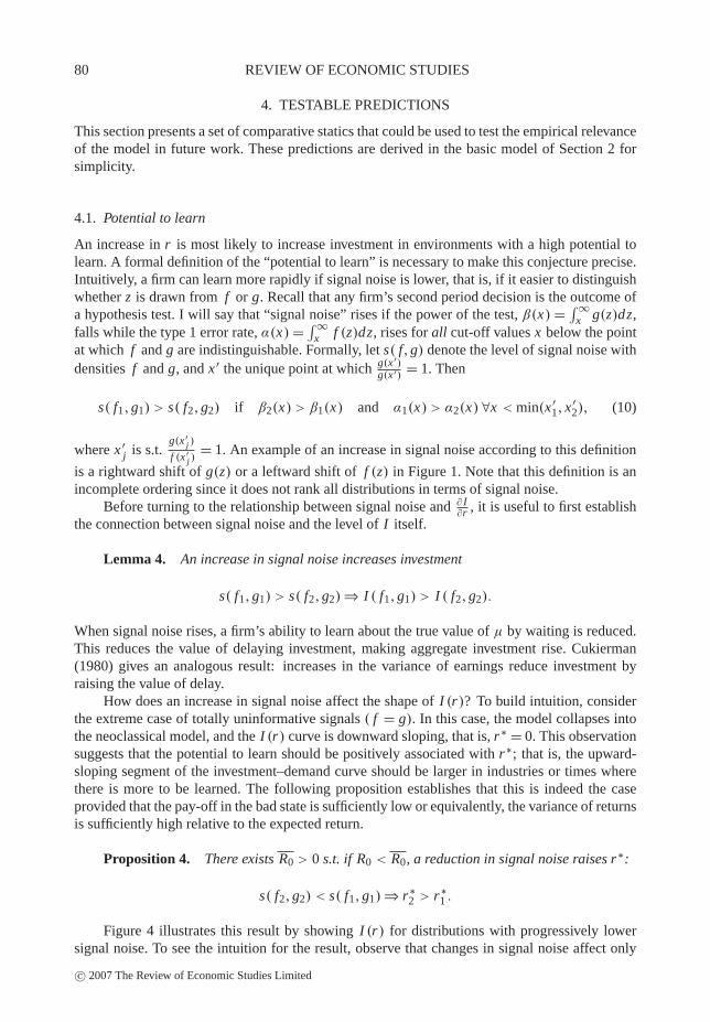
An increase in r is most likely to increase investment in environments with a high potential tolearn. A formal definition of the “potential to learn” is necessary to make this conjecture precise.Intuitively, a firm can learn more rapidly if signal noise is lower, that is, if it easier to distinguishwhether z is drawn from f or g. Recall that any firm’s second period decision is the outcome ofa hypothesis test. I will say that “signal noise” rises if the power of the test, β(x) = ∫ ∞

x g(z)dz,falls while the type 1 error rate, α(x) = ∫ ∞

x f (z)dz, rises for all cut-off values x below the pointat which f and g are indistinguishable. Formally, let s( f,g) denote the level of signal noise withdensities f and g, and x ′ the unique point at which g(x ′)

g(x ′) = 1. Then

s( f1,g1) > s( f2,g2) if β2(x) > β1(x) and α1(x) > α2(x) ∀x < min(x ′1, x ′

2), (10)

where x ′j is s.t.

g(x ′j )

f (x ′j )

= 1. An example of an increase in signal noise according to this definition

is a rightward shift of g(z) or a leftward shift of f (z) in Figure 1. Note that this definition is anincomplete ordering since it does not rank all distributions in terms of signal noise.

Before turning to the relationship between signal noise and ∂ I∂r , it is useful to first establish

the connection between signal noise and the level of I itself.

Lemma 4. An increase in signal noise increases investment

s( f1,g1) > s( f2,g2) ⇒ I ( f1,g1) > I ( f2,g2).

When signal noise rises, a firm’s ability to learn about the true value of µ by waiting is reduced.This reduces the value of delaying investment, making aggregate investment rise. Cukierman(1980) gives an analogous result: increases in the variance of earnings reduce investment byraising the value of delay.

How does an increase in signal noise affect the shape of I (r)? To build intuition, considerthe extreme case of totally uninformative signals ( f = g). In this case, the model collapses intothe neoclassical model, and the I (r) curve is downward sloping, that is, r∗ = 0. This observationsuggests that the potential to learn should be positively associated with r∗; that is, the upward-sloping segment of the investment–demand curve should be larger in industries or times wherethere is more to be learned. The following proposition establishes that this is indeed the caseprovided that the pay-off in the bad state is sufficiently low or equivalently, the variance of returnsis sufficiently high relative to the expected return.

Proposition 4. There exists R0 > 0 s.t. if R0 < R0, a reduction in signal noise raises r∗:

s( f2,g2) < s( f1,g1) ⇒ r∗2 > r∗

1 .

Figure 4 illustrates this result by showing I (r) for distributions with progressively lowersignal noise. To see the intuition for the result, observe that changes in signal noise affect only



Notes: This figure shows I (r) for four pairs of signal distributions f and g. The distributionsare normal with a mean of µ0 for f and µ1 for g and a standard deviation of 16. Otherparameters are the same as those in Figure 2.

FIGURE 4

Signal noise and I (r)

V (l), leaving V (i) unaffected for each firm. An increase in r is more likely to raise an aggregateinvestment if it tends to reduce V (l) more than V (i), making immediate investment preferable.When signal uncertainty is lowered, V (l) changes in two ways. First, firms have a higher prob-ability of investing in the good state in period 2 (β rises). Second, firms have a lower probabilityof investing in the bad state (α falls). The first effect makes expected period 2 profits more sensi-tive to the interest rate, since there is a higher probability of earning revenues in the good state.The second effect goes in the opposite direction, since there is a lower probability of earningrevenues in the bad state.

If R0 is small, the second effect is small in magnitude relative to the first, and so V (l) ismore sensitive to r overall. For instance when R0 = 0, an increase in r has no effect at all onrevenues in the bad state. Therefore, provided that R0 is low, an increase in r is more likely toreduce V (l) relative to V (i) for each firm and thereby raise aggregate investment when signaluncertainty is lower. The low R0 condition on the result requires that the variance of earnings behigh relative to the mean profit rate, which is essentially a requirement that information about thestate of demand is valuable.

4.2. Short run vs. long run

I now turn to the effects of changes in r on total investment over a longer horizon, taking intoaccount changes in investment behaviour beyond the current period. For this analysis, it is neces-sary to consider the T period formulation of the model instead of the two-period special case



discussed above. In this model, the firm has the option to delay investment in every period from1 to T −1.14

In the T -period model, total investment from period 1 to t is given by

I1,t =t∑

s=1

Is =1∫

λ∗0

Cdη(λ0)+t∑

n=2

λ∗0∫

0

P1(Is | λ0)Cdη(λ0) (11)

where P1(Is | λ0) is the probability that a firm with prior λ0 ends up investing in period s. Thenext proposition analyses the relationship between I1,t and r .

Proposition 5.

(i) I1,t (r) is a backward-bending function of r ∀t < T:

r∗1,t ≡ argmax

rI1,t (r) > 0 and r < r∗

1,t ⇒ ∂ I1,t

∂r> 0 and r > r∗

1,t ⇒ ∂ I1,t

∂r< 0

(ii) The upward-sloping portion of the I1,t (r) curve becomes smaller as t rises:

r∗1,t > r∗

1,t+1.

The first part of the proposition is driven by the same two effects that make the responseof investment demand in period 1 to a change in r non-monotonic. If r = 0, all the firms willpostpone their decision until T and I1,t (r = 0) = 0. Similarly, if r is large, I1,t = 0. Hence,investment over the first t periods is maximized at intermediate interest rates.

To understand the second result, observe that the growth in profits from delay diminishesover time because the marginal return to information falls as more knowledge is accumulated.When r falls, investors may delay investment for a few periods to acquire information, but even-tually acquire enough information that further delay is undesirable. Since reductions in r generatetemporary delays in investment, the conventional cost of capital effect starts to dominate at lowerlevels of r in the long run. Consequently, the investment-maximizing r∗

1,t falls with t .15

Proposition 5 implies that the long-run elasticity of investment demand is more negativethan the short-run elasticity of investment demand when firms learn over time. If the near-zeroexisting estimates of the short-run interest elasticity of investment demand are due to learningeffects, interest rate reductions from policies that stimulate savings could, nonetheless, increaseinvestment over a longer horizon.

4.3. Average profit rates

In the neoclassical model, a higher interest rate increases the average rate of return of investmentsthat are undertaken by driving out low NPV ventures. This result is also modified when firmslearn over time.

To analyse the average rate of return, we must identify the level of ex post profitable (µ = 1)and ex post unprofitable (µ = 0) investment by specifying how frequently a project that a managerexpects to succeed with probability λ0 actually does succeed. A natural benchmark is rational

14. See Lemma 1A in the Appendix for a characterization of optimal investment behaviour in the T -period model.15. Unlike learning effects, which die away in the long run as firms acquire perfect information, composition effects

may never subside. Hence, when composition effects are permitted (as in Section 3.2), the long-run investment demandcurve can have a substantial upward-sloping segment.



expectations: Pλ0 [µ = 1] = λ0. In this case, the average (net) profit rate among investments thatare undertaken in period 1 is given by:

ρ(r) =∫ 1λ∗

0λ0(R1 −C)+1(1−λ0)(R0 −C)dη(λ0)∫ 1

λ∗0Cdη(λ0)

. (12)

Proposition 6. The average profit rate ρ is a backward-bending function of theinterest rate:

r < r∗ ⇒ ∂ρ

∂r> 0 and r > r∗ ⇒ ∂ρ

∂r< 0.

As established in Proposition 1, when r < r∗, an increase in the interest rate draws the marginalinvestor with prior λ∗

0(r) into the period 1 pool of investors. This firm has the lowest probabilityof success among the set of firms who are investing. Consequently, it pulls down the average rateof return in the overall pool. Conversely, when r > r∗, an increase in r eliminates the marginalinvestor with prior λ∗

0(r), who has the lowest probability of success in the pool of investors,increasing the average rate of return. The average observed profit rate on current investment isthus a backward-bending function of r . Building on earlier results, an increase in the interest rateis more likely to lower the average observed rate of return when the potential to learn is greaterand in the short run relative to the long run.

4.4. Temporary interest rate and tax changes

I now discuss a few comparative statics for temporary interest rate changes. Formal statementsare omitted since these results are simple extensions of the preceding propositions.

First, consider the effect of an unanticipated temporary increase in the interest rate. Let r1t

denote the per-period interest rate between periods 1 and t < T . An unanticipated increase in r1t

(holding the interest rate fixed in all other periods) is more likely to reduce current investmentthan a permanent increase in r because one can take advantage of lower future costs of capital bydelaying investment. If the potential to learn is sufficiently high, I (r1t ) is backward bending, witha smaller upward-sloping segment than I (r). When the potential to learn is low, I (r1t ) is strictlydownward sloping. The longer the duration of an interest rate change, the less the incentive topostpone investment following a temporary increase, and the larger the range of parameters overwhich I (r1t ) is upward sloping.

Now consider the effect of a temporary anticipated change in the interest rate that beginsin period s > 1 and lasts until period t > s. An anticipated increase in rst is more likely to raisecurrent investment than a permanent change in r because one can take advantage of lower currentcosts of capital by investing immediately. In fact, if the change is anticipated sufficiently far inadvance, current investment may be a strictly upward-sloping function of rst . In contrast, futureinvestment falls when rst rises because of the inter-temporal substitution.

Together, these results indicate that the shape of the yield curve on bonds—which embodiesinvestors’ expectations of future interest rates—should have a significant effect on current andfuture investment. When the yield curve becomes steeper, current investment should rise relativeto subsequent investment.

A final set of predictions relates to the effect of tax changes. In the neoclassical model,taxes matter only through the user cost of capital. In irreversible investment models, both theuser cost and the discount rate matter, and different tax policies may affect these two quantitiesdifferently. For example, accelerated depreciation provisions change the user cost but not thediscount rate, since there is no additional incentive to delay from accelerated depreciation itself.



Hence, accelerated depreciation should unambiguously raise investment. In contrast, changes incapital income taxation affect equilibrium interest rates, thereby changing the discount rate anduser cost simultaneously, with potentially non-monotonic effects on investment.

5. CONCLUSION

This paper has explored the effect of interest rates on investment in an environment where firmsmaking irreversible investments learn over time. The main result is that at low rates, an increasein r increases investment demand by enlarging the set of projects for which r exceeds the returnto delay.

The empirical relevance of the model for explaining how interest rate changes affect aggre-gate investment depends on the extent to which firms re-time investments in response to changesin market conditions. There is some evidence that firms delay investment when faced with in-creased uncertainty, as predicted by irreversible investment models (e.g. Leahy and Whited, 1996;Bulan, Mayer and Somerville, 2004; Bloom, Bond and Reenen, 2006). There is also some evi-dence that cross-sectional variation in interest rates are related to the speed of real estate devel-opment (Capozza and Li, 2001), and time-series fluctuations in interest rates affect the timingof IPO decisions (Jovanovic and Rousseau, 2004). In future work, it would be interesting to testwhether exogenous interest rate changes affect the timing and profitability of irreversible invest-ments in high-risk industries.

APPENDIX

All proofs for the baseline case (Section 2) are given in a model with an arbitrary decision horizon T . The corres-ponding results discussed in the text are for the T = 2 case, unless otherwise noted. We begin by restating Lemma 1 (theoptimal investment rule when T = 2) for arbitrary T in Lemma 1A.

Lemma 1A (Optimal Investment Rule in the T period model). Let λt−1 denote the firm’s prior in period t. Inperiod T , the firm invests iff zT−1 > z∗

T−1 where z∗T−1 satisfies

g(z∗T )

f (z∗T )

= 1−λT−1

λT−1

−πT (0)

πT (1). (1)

In any period t < T , the firm invests iff Vt (i) > Vt (l):

Vt (i) = λt−1πt (1)+ (1−λt−1)πt (0) (2)

Vt (l) =T∑

s=t+1

λt−1 Pt (Is | µ = 1)πs (1)+ (1−λt−1)Pt (Is | µ = 0)πs (0) (3)

whereλt

1−λt= λ0

1−λ0

g(z1, . . . , zt )

f (z1, . . . , zt )= λ0

1−λ0

g(z1) · · ·g(zt )

f (z1) · · · f (zt )(4)

and ∀t > 0: z∗t (z1, . . . , zt−1) is uniquely defined by

Vt (i, z∗t ,λt−1) = Vt (l, z∗

t ,λt−1)

and

Pt (It+1 | µ = 1) =∞∫

z∗t

g(zt )dzt

Pt (It+1 | µ = 0) =∞∫

z∗t

f (zt )dzt



and ∀s ∈ {t +2,. . ., T }:

Pt (Is | µ = 1) =z∗t∫

−∞

z∗t+1∫

−∞·· ·

z∗s−2∫−∞

∞∫

z∗s−1

g(zs−1)dzg(zs−2)dz · · ·g(zt+1)dzg(zt )dz

Pt (Is | µ = 0) =z∗t∫

−∞

z∗t+1∫

−∞·· ·

z∗s−2∫−∞

∞∫

z∗s−1

f (zs−1)dz f (zs−2)dz · · · f (zt+1)dz f (zt )dz.

Proof of Lemma 1A. Period T. Bayes rule and the assumption that zt ⊥ zs for t �= s directly imply equation (4).In period T , the pay-off to investing VT (i) is computed using the updated belief λT (z) about the probability with whichµ = 1 occurs. The firm invests iff VT (i) > 0 ⇒ λT (z)

1−λT (z) >−πT (0)πT (1) . This results in the period T decision rule in (1) using

(4) and the assumption that g(z)f (z) is monotonically increasing.

Period T −1. The remainder of the proof is done by backward induction starting with period T −1, where the firmis faced with a two-period decision problem. First, note that VT−1(i) is computed simply by taking an expectation overthe πT−1 function. To compute VT−1(l), integrate the expected pay-off in period T over the prior density of z:

VT−1(l) =∞∫

−∞max(VT (d1),VT (i))dm(z) =

z∗∫−∞

VT (d1)+∞∫

z∗VT (i)dm(z) (5)

where dm(z) = λ0g(z)+ (1−λ0) f (z) is the unconditional density on z.

⇒ VT−1(l) = λ0πT (1)

∞∫

z∗TD −1

g(z)dz + (1−λ0)πT (0)

∞∫

z∗TD −1

f (z)dz. (6)

Next, I establish that the firm follows a threshold rule for investment in period T −1: ∃ unique z∗T−2(z1, . . . , zT−3)

defined by VT−1(i, z∗T−2,λT−3) = VT−1(l, z∗

T−2,λT−3) s.t. that investing is optimal iff zT−2 > z∗T−2. It is sufficient

to show that ∃ unique λ∗T−2 s.t. VT−1(i,λ∗

T−2) = VT−1(l,λ∗T−2) and that λT−2 > λ∗

T−2 makes investing optimal. Tosee that there is a unique λT−2, rewrite:

VT−1(i) = λT−2b + (1−λT−2)a

VT−1(l) = λT−2b′ + (1−λT−2)a′,

where a = πT−1(0), a′ = PT−1(IT | µ = 0)πT (0), b = πT−1(1), and b′ = PT−1(IT | µ = 1)πT (1).Note that VT−1(l,λT−1 = 0) = 0 > VT−1(i,λT−1 = 0). By assumption, ∃λT−1 s.t. VT−1(l,λT−1) ≤

VT−1(i,λT−1)

By the Intermediate Value Theorem, ∃λ∗T−2 s.t. VT−1(i,λ∗

T−2) = VT−1(l,λ∗T−2).

Since∂VT−1(l)∂λT−2

> 0, it follows that VT−1(l,λ∗T−2) > 0. Now observe that

∂{VT−1(i)− VT−1(l)}∂λT−2

∣∣∣∣λ∗

T−2

= b −a +a′ −b > 0

because Vs (i,λ∗T−2) = Vs (l,λ∗

T−2) ⇔ λ∗T−2b + (1−λ∗

T−2)a = λ∗T−2b′ + (1−λ∗

T−2)a′ > 0.Therefore, at any λ∗

T−2, we must have

∂{VT−1(i)− VT−1(l)}∂λT−2

∣∣∣∣λ∗

T−2

> 0,

which implies that λ∗T−2 is unique. Hence VT−1(i,λT−2) > VT−1(l,λT−2) iff λT−2 > λ∗

T−2.Induction. Finally, I show that when Vt+1(·) has the form in (2) and (3), Vt (·) also has the same form. Vt (i) is easily

computed. To compute Vt (l), recall that the firm invests in period t +1 iff zt > z∗t , where z∗

t has already been computed.



Therefore

Vt (l) =∞∫

z∗t

[λtπt+1(1)+ (1−λt )πt+1(0)][λt−1g(zt )+ (1−λt−1) f (zt )]dzt

+z∗t∫

−∞Vt+1(l,λt )[λt−1g(zt )+ (1−λt−1) f (zt )]dzt

=T∑

s=t+1

λt−1 Pt (Is | µ = 1)πs (1)+ (1−λt−1)Pt (Is | µ = 0)πs (0). (7)

Finally, arguments analogous to those given above establish that ∃ unique z∗t−1 s.t.

Vt−1(i, z∗t−1,λt−2) = Vs (l, z∗

t−1,λt−2)

and that if zt−1 > z∗t−1 the investor will invest in period t . This completes the induction. ‖

Proof of Lemma 2. The proof follows directly from the second step of Lemma 1A. In any period t , ∃ unique λ∗t−1

s.t. Vt (i,λ∗t−1) = Vt (l,λ∗

t−1) and that λt−1 > λ∗t−1 ⇔ Invest. Applying this to t = 1 gives the result. ‖

Proof of Lemma 3. In period 2, a firm invests if λ1 p21+r > C . Since ∂p2

∂ I c2

< 0, it follows that there is a unique cut-off

value λ∗1 and a corresponding price p2(I c

2 (λ∗1)) such that

λ∗1 p2(I c

2 (λ∗1))

1+ r= C. (8)

In equilibrium, all firms with λ1 > λ∗1 invest, all other firms stay out, and the market clears at the resulting price p2 by

construction. Therefore, for any firm with given prior λ0, there is a cut-off value z∗(λ0) such that the firm invests inperiod 1 iff z > z∗.

Now consider period 1 investment behaviour. Firms invest in period 1 if

V (i,λ0) = λ0 p1

1+ r−C (9)

> V (l,λ0) = λ0β(z∗(λ0))

[p2

(1+ r)2− C

1+ r

]+ (1−λ0)α(z∗(λ0))

[− C

1+ r

](10)

where α and β are defined as in the text. Note that V (l,λ0) is strictly positive in equilibrium if λ0 > 0. It follows fromLemma 2 that for a given price vector (p1, p2), there is a unique λ∗

0 such that firms with λ0 > λ∗0 invest in period 1 and

the remainder delay. Since ∂pt/∂ I ct < 0, ∂λ∗

0/∂p1 < 0, and ∂λ∗0/∂p2 > 0, there is a unique price vector (p1, p2) at which

all firms are optimizing and markets clear in both periods. Thus, equilibrium investment is characterized by a price vector(p1, p2) and a cut-off value λ∗

0 such that

V (i,λ∗0, p1) = V (l,λ∗

0, p1, p2) > 0. ‖ (11)

Proof of Lemma 4. Take any ( f1,g1), ( f2,g2) s.t. s( f1,g1) > s( f2,g2). For the firm with λ′0 = λ∗

0( f1,g1),

V1(l) =T∑

s=2

λ0 P1(Is | µ = 1)πs (1)+ (1−λ0)P1(Is | µ = 0)πs (0) (12)

V (i,λ′0) = λ′

0

{R1

1+ r−C

}+ (1−λ′

0)

{R0

1+ r−C

}. (13)

The shift from ( f1,g1) to ( f2,g2) only affects V (l,λ′0). It follows from the definition of a reduction in signal noise that

for any s, P1(Is | µ = 1) is higher under ( f2,g2) than under ( f1,g1), while P1(Is | µ = 0) is lower. Hence,

V (l,λ′0; f2,g2) > V (l,λ′

0; f1,g1) = V (i,λ′0). (14)



Lemma 2 implies that λ∗0( f2,g2) > λ′

0 = λ∗0( f1,g1). Since ∂ I

∂λ∗0

< 0, the result follows. ‖

Proof of Proposition 1.

(i) Equations (2) and (3) imply that in period 1

V (i) = λ0π1(1)+ (1−λ0)π1(0) (15)

V (l) =T∑

s=2

λ0 P1(Is | µ = 1)πs (1)+ (1−λ0)P1(Is | µ = 0)πs (0) (16)

where πt (µ) = Rµ

(1+r )t− C

(1+r)t−1 . Now suppose r = 0. Then

V (i) = λ0{R1 −C}+ (1−λ0)(R0 −C)

V1(l,λ0) = λ0{R1 −C}T∑

t=2

P1(It | µ = 1)+ (1−λ0){R0 −C}T∑

t=2

P1(It | µ = 0).

For λ0 = 1, the definitions in Lemma 2 imply that z∗t = ∞ for t < T and z∗

T = −∞ ⇒ ∑Tt=2 P1(It | µ = 1) = 1.

Therefore λ0 = 1 ⇒ V (i,λ0) = (π1 − δ) = V (l,λ0). Hence λ∗0(r = 0) = 1 ⇒ I (r = 0) = 0.

To establish that limr→0∂ I∂r (r) = +∞, note first that ∂ I

∂r = ∂ I∂λ∗

0× ∂λ∗

0∂r .

By the Implicit Function Theorem,

∂λ∗0

∂r= − ∂V (i ,λ0)/∂r − ∂V (l,λ0)/∂r

∂V (i ,λ0)/∂λ0 − ∂V (l,λ0)/∂λ0

∣∣∣∣λ∗

0

. (17)

Let∂λ∗

0∂r = N (r)

D(r) . It can be shown that N (r = 0) = C − R1 < 0 and D(r) > 0 ∀r > 0.

Since D(r = 0) = 0 and ∂ I∂λ∗

0= −λ∗

0dη(λ∗0) < 0 it follows that limr→0

∂ I∂r (r) = +∞.

(ii) Note that C < R1 ⇒ ∃r ′ s.t. R11+r ′ = C . Then

r ≥ r ′ ⇒ V (i,λ0) < 0 ∀λ0 ≤ 1 ⇒ λ∗0(r) = 1 ⇒ I (r) = 0.

Given that (i) I (0) = I (r ′) = 0, (ii) I (r) is continuous, and (iii) [0,r ′] is compact, it follows that I (r) has aninterior maximum r∗ ∈ (0,r ′).To prove uniqueness of r∗, recall

∂ I

∂r= ∂ I

∂λ∗0

× ∂λ∗0

∂r= ∂ I

∂λ∗0

N (r)

D(r). (18)

Since I is continuous and ∂V (i ,λ0)−∂V (l,λ0)∂λ0

(λ∗0) > 0 ∀r > 0, N (r) = 0 at any critical r . A sufficient condition

for r∗ to be unique is that N (r) has a unique root. I establish this by showing that N (r) = 0 ⇒ ∂N∂r (r) > 0.

Given that ∂V (l)−∂V (i)∂r (r∗) = 0 and V (l,λ∗

0(r∗)) = V (i,λ∗0(r∗)), it follows that

∂N

∂r(r∗,λ∗

0(r∗)) = 1

1+ r∗ ∂

[(1+ r)(∂V (l)− ∂V (i))

∂r

]/∂r = 1

1+ r∗ ∂[M(r)]/∂r (19)

where

M(r) = ∂((1+ r)V (l))(−∂((1+ r)V (i))

∂r(20)

= −λ0β(z∗)R1

(1+ r)2− (1−λ0)α(z∗)

R0

(1+ r)2+C,

and

β ≡T∑

t=2

P1(It | µ = 1)

(1+ r)t−1, α ≡

T∑t=2

P1(It | µ = 0)

(1+ r)t−1.



Differentiating (20) gives

∂[M(r)]/∂r = λ0β(z∗)2R1

(1+ r)3+ (1−λ0)α(z∗)

2R0

(1+ r)3− ∂β

∂r

R1

(1+ r)2− ∂α

∂r

R0

(1+ r)2. (21)

To sign (21), note that ∂α∂r (r∗) < 0 and ∂β

∂r (r∗) < 0. This is easiest to see when T = 2, where

∂β

∂r= − ∂z∗

∂rg(z∗),

∂α

∂r= − ∂z∗

∂rf (z∗).

Note that ∂z∗∂r > 0 because g(z∗)

f (z∗) = 1−λ0λ0

C−R0/(1+r)R1/(1+r)−C and ∂[ g(z)

f (z) ]/∂z > 0. Therefore ∂α∂r < 0 and ∂β

∂r < 0.

When T > 2, the final step can be established using ∂ P1(It |λ0)∂r (r∗) < 0 ∀t > 1, which follows from

∂2{V (l,λ0)−V (i,λ0)}∂λ0∂r < 0 (see proof of Proposition 4 below) and the definition of P1(It |λ0). Since ∂α

∂r < 0 and∂β∂r < 0, it follows that ∂M(r)/∂r(r∗) > 0 ⇒ ∂N (r)/∂r(r∗) > 0. ‖

Proof of Proposition 2. Define p = λ0 p1 + (1 − λ0)p0 as the expected price ex ante and note that p =∫ ∞z=−∞{λ1(z)p1 + (1−λ1(z))p0}dm(z) where dm(z) denotes the marginal distribution of z, as defined in the text.

In period 2, after observing z, the firm updates its beliefs to λ1(z) and chooses I2(z) to

max{λ1(z)p1 + (1−λ1(z))p0} F(I1 + I2)− F(I1)

(1+ r)2− I2(z)

1+ rs.t. I2 ≥ 0. (22)

Let I∗2 (z) denote the optimal level of period 2 investment as a function of z. At an interior optimum, optimal

investment I∗2 (z) satisfies:

F ′(I1 + I∗2 (z)){λ1(z)p1 + (1−λ1(z))p0} = 1+ r. (23)

When F ′(I1){λ1(z)p1 + (1−λ1(z))p0} < 1+ r , I∗2 (z) = 0.

The value function in period 2 is

V2(I1) =∞∫

z=−∞

[{λ1(z)p1 + (1−λ1(z))p0} F(I1 + I∗

2 (z))− F(I1)

(1+ r)2− I∗

2 (z)

1+ r

]dm(z). (24)

The value function in period 1 is:

V1 = pF(I1)

1+ r− I1 + V2(I1)

=∞∫

z=−∞[λ1(z)p1 + (1−λ1(z))p0]

[F(I1)

1+ r+ F(I1 + I2(z))− F(I1)

(1+ r)2

]− I2(z)

1+ r− I1dm(z).

(25)

Given the optimality condition for I∗2 (z), it follows that

∂V1(r = 0)

∂ I1=

∞∫z=−∞

[λ1(z)p1 + (1−λ1(z))p0][F ′(I1 + I∗2 (z))−1]dm(z) < 0

since for z sufficiently small, F ′(I1){λ1(z)p1 + (1−λ1(z))p0} < 1. Hence V1(r = 0) is maximized when I1(r = 0) = 0.It is easy to show that as r → ∞, I1 → 0 and that ∃r ′ > 0 s.t. I1(r ′) > 0. These observations, coupled with continuity

of I1(r), establish the result. ‖

Proof of Proposition 3. Observe that ∂ I1∂r = d I1

dλ∗0

dλ∗0

dr . The implicit function theorem implies

dλ∗0

dr= − dV (i,λ0)/dr −dV (l,λ0)/dr

dV (i,λ0)/dλ0 −dV (l,λ0)/dλ0= − N

D. (26)

At r = 0, the denominator of this expression is

D = p1 −β(λ∗0)p2 + (β(λ∗

0)−α(λ∗0))C.



Since β > α and p1 > p2, it follows that D > 0. The numerator is

N = − λ0 p1

(1+ r)2+ λ0dp1/dr

1+ r−

{λ0β

(−2

p2

(1+ r)3+ dp2/dr

(1+ r)2+ C

(1+ r)2

)+ (1−λ0)α

(C

(1+ r)2

)}. (27)

Using the fact that V (i,λ∗0) = V (l,λ∗

0), N simplifies at r = 0 to

N (r = 0)|p-fixed = λ∗0(r = 0)β(λ∗

0)p2 −C

if dpt/dr is 0.I now show that N (r = 0)|p-fixed �⇒ ∂ I

∂r (r = 0) > 0 using a proof by contradiction. Suppose that ∂ I1∂r (r = 0) < 0.

In this case, dp1/dr > dp2/dr > 0 because ∂ I c1/∂ I1 = 1 and ∂ I c

2/∂ I1 < 1 and ∂pt/∂ I ct < 0. It follows that N (r = 0) > 0

when p is variable. Since N > 0 and D > 0,dλ∗

0dr < 0, which implies ∂ I1

∂r (r = 0) > 0. But this contradicts the supposition.

Therefore ∂ I1∂r (r = 0) > 0 if N (r = 0)|p-fixed > 0.

Since λ∗1 p2 = C(1+ r) in period 2 equilibrium, N (r = 0)|p-fixed > 0 if

λ∗0β(λ∗

0)

λ∗1

> 1. Hence

λ∗0β(λ∗

0)

λ∗1

> 1 �⇒ ∂ I1

∂r(r = 0) > 0. ‖

Corollary to Proposition 3. At r = 0, the period 2 threshold for investment is characterized by the followingcondition:

λ∗1 = C0 + 1

2 K

h(I c2 )+ K

.

Since I c2 is bounded, it follows that

limK→∞λ∗

1 = 1

2.

I now establish that raising K lowers period 1 investment using a proof by contradiction. Consider the behaviour of themarginal period 1 firm, with λ0 = λ∗

0. At the original equilibrium, the marginal investor has

V (i,λ0) = λ0

(h(I c

1 )+ 1

2K −C0

)+ (1−λ0)

[−

(C0 + 1

2K

)](28)

= V (l,λ0) = λ0β(z∗(λ0))

[(h(I c

2 )+ K )−(

C0 + 1

2K

)]+ (1−λ0)α(z∗(λ0))

[−

(C0 + 1

2K

)]. (29)

Suppose that increasing K raises I1. This would require that dV (i,λ0)/dK > dV (l,λ0)/dK . Recall that ∂ I c1/∂ I1 = 1

and ∂ I c2/∂ I1 < 1. Hence, ∂h/∂ I c

t < 0 implies ∂V (i,λ0)/∂ I1 < ∂V (l,λ0)/∂ I1. In addition, observe that ∂V (i,λ0)/∂K <

∂V (l,λ0)/∂K because β > α. Consequently, both the direct effect of increasing K and the indirect effect of equilibriumprice changes lower V (i,λ0) relative to V (l,λ0) for the marginal investor. This makes the marginal firm drop out of theperiod 1 investment pool, lowering I1. But this contradicts the supposition. Therefore increasing K must strictly lowerI1. Hence, as K → ∞, λ∗

0 → 1, while implies β(λ∗0) → 1. Meanwhile λ∗

1 → 12 . It follows that (9) must hold as K → ∞,

as claimed. ‖

Proof of Proposition 4. Take any ( f1,g1) and ( f2,g2) s.t. s( f2,g2) < s( f1,g1). Let r∗1 and r∗

2 denote the

investment-maximizing values of r in each case, and let λ′0 = λ∗

0(r = r∗1 , f1,g1) and λ

′′0 = λ∗

0(r = r∗1 , f2,g2). By Lemma

4, λ′′0 > λ′

0.It can be shown that

∂2{V (l,λ0)− V (i,λ0)}∂λ0∂r

= ∂

{(R1

(1+ r)2− C

1+ r

)β(z∗)−

(R0

(1+ r)2− C

1+ r

)α(z∗)

−((

R1

1+ r−C

)−

(R0

1+ r−C

))}/∂r < 0.

Since∂V (l,λ′

0; f1,g1)

∂r = ∂V (i,λ′0; f1,g1)

∂r at r = r∗1 , it follows that

∂V (l,λ′′0 ; f1,g1)

∂r <∂V (i,λ′′

0 ; f1,g1)

∂r at r = r∗1 .



Using logic similar to that in Lemma 4, s( f2,g2) < s( f1,g1) ⇒ β2 > β1 and α2 < α1. Observe that

∂V (l)

∂r= −λ0β

{2R1

(1+ r)3− C

(1+ r)2

}− (1−λ0)α

{2R0

(1+ r)3− C

(1+ r)2

}.

If R0 < C/2, both terms become more negative when β rises and α falls; hence

∂V (l,λ′′0 ; f2,g2)

∂r<

∂V (l,λ′′0 ; f1,g1)

∂r<

∂V (i,λ′′0 ; f1,g1)

∂r= ∂V (i,λ′′

0 ; f2,g2)

∂r

⇒ ∂ I

∂r(r = r∗

2 ; f1,g1) = ∂ I

∂λ∗0

× ∂V (l,λ0)/∂r − ∂V (i ,λ0)/∂r

∂V (i ,λ0)/∂λ0 − ∂V (l, λ0)/∂λ0

∣∣∣∣λ′′

0

> 0.

Therefore R0 < C/2 ⇒ r∗1 > r∗

2 by Proposition 1. ‖

Proof of Proposition 5.

(i) For any t < T , r = 0 ⇒ λ∗0 = 1 and z∗

1 = z∗2 = . . . = z∗

t = ∞ by Lemma 1A.

Therefore I1,t (r = 0) = 0. As above, I1,t (r) = 0 for r > r ′ > 0 for r ′ s.t. R11+r ′ = C .

By the Intermediate Value Theorem, ∃r∗1,t that is a critical point and global maximum for I1,t .

Uniqueness of r∗1,t follows from an argument equivalent to that given in Proposition 1 to show that r < r∗

1,t ⇔∂ I1,t∂r > 0.

(ii) I will show that,∂ I1,t∂r (r) < 0 ⇒ ∂ I1,t+1

∂r (r) < 0, which establishes the result. Observe that

I1,t (r) =t∑

s=1

Is (r) =1∫

λ*0

C dη(λ0)+t∑

s=2

λ*0∫

0

P1(Is | λ0)C dη(λ0). (30)

Therefore

∂ I1,t

∂r= − ∂λ∗

0∂r

Cdη(λ∗0)

⎧⎨⎩1−

t∑s=2

1

(1+ r)s−1P1(Is | λ∗

0)

⎫⎬⎭+C

λ*0∫

0

⎡⎣ t∑

s=2

∂ P1(Is | λ0)

∂r

⎤⎦dη(λ0). (31)

Now suppose r > r∗, the investment-maximizing interest rate for period 1. Then∂λ∗

0∂r > 0 implies the first term is

negative in the expression above. To evaluate the sign of the second term, note that ∂ P1(It |λ0)∂r < 0 ∀λ0 < λ∗

0 when

r > r∗. This follows from ∂2{V (l,λ0)−V (i,λ0)}∂λ0∂r < 0 and the definition of P1(It | λ0). Since P1(It | λ0) > 0 ∀t > 1

and ∂ P1(It |λ0)∂r < 0 ∀t > 1, it follows by inspection that

∂ I1, t∂r (r) < 0 ⇒ ∂ I1,t+1

∂r (r) < 0. ‖

Proof of Proposition 6. Define ρ(r) = ∫ 1λ*

0λ0(R1 −C)+ (1−λ0)(R0 −C))dη(λ0)/

∫ 1λ*

0Cdη(λ0).

Note that

∂ρ/∂r =(

− ∂λ∗0

∂r

)Cdη(λ∗

0)

[∫ 1λ*

0Cdη(λ0)]2

A, (32)

where

A =1∫

λ*0

[λ∗0(R1 −C)+ (1−λ∗

0)(R0 −C)]− [λ0(R1 −C)+ (1−λ0)(R0 −C)]dη(λ0). (33)

Since∫ 1λ*

0(λ*

0 −λ0)dη(λ0) < 0, it follows that A < 0. Hence r < r∗ ⇒ ∂λ∗0

∂r < 0 ⇒ ∂ρ∂r < 0 and r > r∗ ⇒ ∂λ∗

0∂r >

0 ⇒ ∂ρ∂r > 0 ‖

Acknowledgements. I thank George Akerlof, Alan Auerbach, Nick Bloom, Gary Chamberlain, V. K. Chetty,Martin Feldstein, Ben Friedman, Jerry Green, Boyan Jovanovic, Anil Kashyap, Michael Schwarz, Arnold Zellner, twoanonymous referees, and the editor for very helpful comments and discussions. Funding from the National Bureau ofEconomic Research and National Science Foundation is gratefully acknowledged.



REFERENCESABEL, A. and EBERLY, J. (1996), “Optimal Investment with Costly Reversibility”, Review of Economic Studies, 63,

581–593.ALCHIAN, A. (1959), “Costs and Outputs”, in M. Abramotvitz (ed.) The Allocation of Economic Resources (Stanford,

CA: Stanford University Press) 160–172.ARROW, K. J. (1968), “Optimal Capital Policy with Irreversible Investment”, in J. N. Wolfe (ed.) Value, Capital and

Growth, Papers in Honour of Sir John Hicks (Chicago: Aldine) 1–19.BERTOLA, G. and CABALLERO, R. J. (1994), “Irreversibility and Aggregate Investment”, Review of Economic Studies,

61, 223–246.BLOOM, N., BOND, S. and REENEN, J. V. (2006), “Uncertainty and Investment Dynamics”, Review of Economic

Studies (forthcoming).BULAN, L., MAYER, C. and SOMERVILLE, T. (2004), “Irreversible Investment, Real Options, and Competition:

Evidence From Real Estate Development” (Mimeo, Columbia University).CABALLERO, R. J. (1999), “Aggregate Investment”, in J. P. Taylor and M. Woodford (eds.) Handbook of Macroeco-

nomics, Vol. 1B (Amsterdam: North-Holland) 813–862.CABALLERO, R. J., ENGEL, E. and HALTIWANGER, J. (1995), “Plant-Level Adjustment and Aggregate Investment

Dynamics”, Brookings Papers on Economic Activity: Macroeconomics, 1–54.CAPOZZA, D. and LI, Y. (1994), “The Intensity and Timing of Investment: The Case of Land”, American Economic

Review, 84, 889–904.CAPOZZA, D. and LI, Y. (2001), “Residential Investment and Interest Rates: An Empirical Test of Development as a

Real Option”, Real Estate Economics, 29, 503–519.CHIRINKO, R. (1993a), “Business Fixed Investment Spending: A Critical Survey of Modelling Strategies, Empirical

Results, and Policy Implications”, Journal of Economic Literature, 31, 1875–1911.CHIRINKO, R. (1993b) Econometric Models and Empirical Findings for Business Investment (New York: Basil

Blackwell).COOPER, R. W. and HALTIWANGER, J. C. (2006), “On the Nature of Capital Adjustment Costs”, Review of Economic

Studies, 73 (3), 611–633.CUKIERMAN, A. (1980), “The Effects of Uncertainty on Investment Under Risk Neutrality with Endogenous Informa-

tion”, Journal of Political Economy, 88 (3), 462–475.DIXIT, A. and PINDYCK, R. (1994) Investment Under Uncertainty (Princeton: Princeton University Press).DOMS, M. and DUNNE, T. (1998), “Capital Adjustment Patterns in Manufacturing Plants”, Review of Economic

Dynamics, 67, 117–145.HAAVELMO, T. (1960) A Study in the Theory of Investment (Chicago: Chicago University Press).JORGENSON, D. (1963), “Capital Theory and Investment Behavior”, American Economic Review Papers and Proceed-

ings, 53 (2), 247–259.JOVANOVIC, B. and ROUSSEAU, P. (2001), “Why Wait? A Century of Life before IPO”, American Economic Review

Papers and Proceedings, 91, 336–341.JOVANOVIC, B. and ROUSSEAU, P. (2004), “Interest Rates and Initial Public Offerings” (NBER Working Paper No.

10298, National Bureau of Economic Research).LEAHY, J. and WHITED, T. (1996), “The Effects of Uncertainty on Investment: Some Stylized Facts”, Journal of Money

Credit and Banking, 28, 64–83.


interest rates, irreversibility, and backward-bending...

Documents