interest rate volatility and monetary policy

Interest Rate Volatility and Monetary PolicyAuthor(s): Carl E. WalshSource: Journal of Money, Credit and Banking, Vol. 16, No. 2 (May, 1984), pp. 133-150Published by: Ohio State University PressStable URL: http://www.jstor.org/stable/1992540 .

Accessed: 05/06/2014 11:45

Your use of the JSTOR archive indicates your acceptance of the Terms & Conditions of Use, available at .http://www.jstor.org/page/info/about/policies/terms.jsp

.JSTOR is a not-for-profit service that helps scholars, researchers, and students discover, use, and build upon a wide range ofcontent in a trusted digital archive. We use information technology and tools to increase productivity and facilitate new formsof scholarship. For more information about JSTOR, please contact [email protected].

.

Ohio State University Press is collaborating with JSTOR to digitize, preserve and extend access to Journal ofMoney, Credit and Banking.

http://www.jstor.org

This content downloaded from 2.103.194.60 on Thu, 5 Jun 2014 11:45:25 AMAll use subject to JSTOR Terms and Conditions

http://www.jstor.org/action/showPublisher?publisherCode=ohiosup

http://www.jstor.org/stable/1992540?origin=JSTOR-pdf

http://www.jstor.org/page/info/about/policies/terms.jsp


CARL E. WALSH

Interest Rate Volatility and Monetary Policy

1. INTRODUCTION

IN OCTOBER 1979, the Federal Reserve.shifted from an interest-rate-oriented operating procedure to a reserves-oriented procedure. One expected result of such a policy shift was an increase in the short-run volatility of market interest rates, and this did occur. However, the increase in interest rate fluctuations was very large, probably much larger than was anticipated. According to a review of monetary control procedures carried out by the Federal Reserve staff (Tinsley et al. 1981), the standard deviation of monthly changes in the federal funds rate increased from 0.27 in the year prior to the policy shift to 2.4 in the year following the shift. Such a large increase suggests that the shift in operating procedures may have induced structural changes in the behavioral relationships which characterize the financial sector This paper investigates that possibility using a simple, rational expectations model. The model implies that a move to an aggre- gates policy induces shifts in the money demand equation which may tend to accentuate the subsequent rise in interest rate volatility. This result is derived by explicitly expressing the variance of interest rates as a function of the monetary policy rule, and then comparing rational expectations equilibria under alternative rules.

*I would like to thank members of the research department of the Federal Reserve Bank of Kansas City, participants in the 1983 Summer Institute of the National Bureau of Economic Itesearch Financial Markets and Monetary Economics program, Alan Blinder, David Germany, John Taylor, and Roger Waud for helpful comments. Part of this research was carried out while the author was a visiting scholar at the Federal Reserve Bank of Kansas City.

CARL E. WALSH is assistant professor of economics, Princeton University.

Journal of Money, Credit, and Banking, Vol. 16, No. 2 (May 1984) Copyright t 1984 by the Ohio State University Press



134 : MONEY, CREDIT, AND BANKING

The argument advanced in this paper is motivated by the following line of reasoning. Models of portfolio choice by risk averse asset holders imply that the demand for risky assets will depend upon the joint probability distribution of asset returns. In a mean-variance framework, for example, this implies that the demand for an asset will be a function of both the expected rates of return on all assets and the covariances among asset returns (Tobin 1958). If the monetary authority changes the way in which it adjusts the money supply in response to shocks to the economy, the covariances between the rate of inflation (the negative of the real return on money) and the returns on other assets will be affected. This will produce a shift in asset demand equations in general, and in the money demand function in particular.

The policy-induced change in the demand for money function is not simply a change in the intercept; interest and income elasticities change. Consequently, the old money demand function cannot be used to draw inferences about the variance of interest rates after a change in the operating procedure. This,- of course, is just another example of the Lucas policy evaluation critique (Lucas 1976).

In principle, one should consider the possible dependence of all the model's behavioral relationships on the policy rule chosen by the monetary authority. The present paper, however, focuses only on the potential dependency of the model's aggregate portfolio balance equation on the policy rule, taking the other equations to be policy invariant. The reason for this is empirical. After the Federal Reserve's change in its operating procedures, the volatility of interest rates over even very short observation periods (e.g., weekly) increased dramatically, so the financial sector would seem to be the most obvious area to examine for possible structural shifts. Shifts in aggregate demand and supply relationships seem less promising as an explanation for the observed rise in short-term interest rate volatility.

The money demand, or portfolio balance, equation in the model is derived from a simple, underlying model of portfolio choice. This derivation shows how the parameters of a standard money demand function are themselves functions of the stochastic properties of the interest rate and the rate of inflation. In the present model, the variance of the nominal price of bonds and the interest elasticity of the demand for money turn out to be the critical variables in solving for the rational expectations equilibrium. In such an equilibrium, the variance of bond prices upon which individuals base their portfolio choices, and which therefore determines the interest elasticity of money demand, must agree with the bond price variance that is implied by the assumption of market clearing. The requirement of market clearing, however, implies that the bond price movements, and hence the variance of bond prices, necessary to maintain money market equilibrium will depend on the interest elasticity of money demand.

After deriving the rational expectations equilibrium, the properties of the equilibrium are discussed and it is shown how the stochastic properties of the price of bonds are influenced by the monetary authority's policy rule. The model implies that a move by the monetary authority from a policy which had attempted to smooth bond price fluctuations to one which pays less attention to bond prices is likely to



CARL E. WALSH : 135

lead to a larger increase in bond price (and hence interest rate) volatility than would have been predicted by a model which assumed the money demand function to be policy invariant. Since the change in policy leads to greater bond price volatility, investors view bonds as riskier assets and they make smaller adjustments in their portfolios in response to changes in the expected rate of return from holding bonds. This, however, means that shocks to the money market will now require larger swings in the price of bonds to clear the market. Hence, in the new equilibrium, bond prices are more volatile than would have been predicted if the interest elasticities of the demands for bonds and money had been assumed to remain constant.

Previous models that have analyzed the effects of alternative monetary policy rules (Poole 1970, Sargent and Wallace 1975, Woglom 1979, McCallum 1981, McCallum and Hoehn 1983) have assumed a policy invariant structure. The present model suggests that such an assumption may be misleading. For example, it is shown that the volatility of the money supply could actually increase if the monetary authority decided to adjust the money supply less in response to a given bond price movement.

The basic model is specified in the next section and the portfolio balance equation is derived from an underlying portfolio choice model. The rational expectations solution is derived in section 3, while the properties of the solution are discussed in section 4. Section 4 also investigates the effects of ignoring the dependence of the parameters of the portfolio balance equation on the policy rule. Section 5 briefly considers the implications for optimal stabilization policy. Finally, section 6 provides a summary of the paper's results.

2. THE BASIC MODEL

There are four equations in the model to be studied: an aggregate supply function, an aggregate demand function, a portfolio balance equation, and a policy rule describing the actions of the monetary authority. Because the focus is on the potential dependence of the portfolio balance schedule on the monetary policy rule, the specifications chosen for the aggregate supply and demand functions are inten- tionally simple. The model structure is also chosen to be basically similar to other aggregate rational expectations models which have been used to evaluate alternative policy rules (e.g., Sargent and Wallace 1975, Woglom 1979, McCallum and Hoehn 1983).

The economy modeled produces a single, nondurable good with the use of labor input; there is, for simplicity, no capital. Workers and firms, based upon their knowledge of the equilibrium stochastic process describing the evolution of the price level, are assumed to negotiate contracts that fix the nominal wage on a period-by-period basis as in Fischer (1977). This nominal wage path would incorporate any predictable component of the price level, but it is assumed that the actual realizations of the unpredictable component of prices will produce variations in the actual real wage. Since money wages are fixed during each period, aggregate




demand disturbances will produce output fluctuations. If the stochastic process describing the equilibrium price level were to change, perhaps as a result of some change in the behavior of the monetary authority, new contracts would be written to reflect any new predictable component of prices.

If p, is the log of the price of output, aggregate supply will be a positive function of P. - .- lP., where 5X, is the expectation of the random variable x, conditional on the information available at s. Assuming aggregate supply is also subject to a serially uncorrelated random shock, the aggregate supply function will be written as

y,=y,+ (x(p,-t-lP.) + >,;(x>O, (1)

where y, is the log of output, y, is a deterministic trend (Y,+ 1 - y, = n), and >, is taken to be normally distributed with mean zero and variance CJb2.

To provide a consistent yet simple structure to the demand side of the economy, assume that an equal number of identical individuals are born eaeh period and live for two periods. An individual born at the beginning of period t supplies one unit of labor services during period t. During period t + 1, the individual is retired and simply consumes his or her total wealth. The lifetime utility of an individual born at time t is assumed to be given by u = U(C,) + E[V(W,+ 1)], where C, is period t consumption, W,+ 1 is wealth at the start of t + 1, and E[ ] is the expectations operator. Individuals will be assumed to be risk averse and further assumptions about the function V( ) will be made below.

There are two financial assets in the model, money and bonds. A basic assumption of this paper is that there exists uncertainty about the nominal rate of return on bonds because their maturity exceeds the planned holding period (in the present case, one period) of individual investors. Assuming, in the context of the present discrete time model, that there exists a nominal one-period bond would eliminate nominal return uncertainty. However, the view taken here is that when all non- money financial assets are aggregated into one asset called a bond, it is best to assume the holding period yield on this bond is viewed as uncertain by investors.

Because the focus in this paper is on structural shifts in the portfolio balance equation, it will simply be assumed that the aggregate consumption function at time t, equal to the wealth of individuals born at t - 1 plus the value of C, chosen to maximize lifetime utility by individuals born at t, results in aggregate demand being a function of the expected real return on bonds and current wealth. 1 If s, denotes the log of the nominal bond price (including any coupon payment), the expected real return is approximated by (,5,+ 1 - .P.+ 1) - (s, - p,). The expected real rate of interest requires expectations of both the future price level and the future price of bonds. Assuming aggregate demand can be approximated by a log-linear relationship yields

lThis assumption parallels that made in standard aggregate models in which savings and portfolio allocation decisions are taken to be made sequentially.



CARL E. WALSH : 137

Yr = 0 + I[(tSt+l-tPr+l) - (5, - p,)] + 2W, + u,' (2)

where w, is the log of wealth, u, is a random shock to demand, l 1 < 0, and 2 > °

The disturbance u, is taken to be normally distributed with mean zero and variance Cr2

The final equation modeling private sector behavior is a portfolio balance, or money demand, equation. In the next section it is shown that both the log of the price level and the log of the price of bonds are normally distributed. Hence, if the nominal rate of return on bonds and the rate of inflation are approximated by (s,+ l

- s,) and (P,+ 1 - p,), respectively, the returns to holding bonds and money will be completely characterized by the first and second moments of their real returns.

Assume then that the expected utility of next period wealth, EV(W,+ I) can be written as a function of EW,+ 1 and var W,+ 1.

EV(W,+1)-J(EW,+1,varW,+1) ( )

Define (x, as the fraction of wealth held in the form of money. Suppose rm,+ 1, to be specified below, is the real return yielded by money and rb,+ l = (s+ l - P.+ I) - (s, - p,) is the real rate of return on bonds. If individuals exhibit constant relative risk aversion, the optimal portfolio allocation is independent of W,. In this case, maximizing (3) is equivalent to maximizing

,zp,+ l -(112)pE,[rp,+ 1-,rp,+ 1]2, (3')

where rp,+ 1 is the return on the total portfolio, here approximated by rm,+ I(Xt +

rbt + 1 ( 1 - (X, ) . 2

Money holdings are assumed to lead to reductions in the transaction costs that individuals incur when engaging in consumption activities. The real return to mon-

ey consists, then, of a return in the form of transaction services yielded by money and a capital gains component resulting from price level changes. For simplicity, the transactions return is taken to be a constant plus a term proportional to the deviation of log real output from trend. In this case

rm.+ 1 = to + (Y.-Y)-(P.+ 1 -P.) . (4)

One could think of X as a function of the variance of individual expenditures within each period (see Santomero and Seater 1981).

2If r = W,+ I/W, is a function of a choice variable x, the first-order condition for the maximization of (3) is gI (8Erpl Ax)W, + J2(8 var rplAx)W,2 = O, or (8Erpl Ax) + ( J2W,/JI )(8 var rpl Ax) = O. If J2W,/JI is constant (constant relative risk aversion), this is the same first-order condition obtained by maximizing Erp - (1/2)pvarrp if p = -2J2W,/JI. This specification of the portfolio choice objective function is not crucial. If utility is a concave function of period t + 1 wealth, expected utility can be approximated by a second-order Taylor expansion around current wealth, producing a first-order condition for expected utility maximization, which leads to an equation similar to equation (6) in the text.




The expected real return on money is ,rm,+ l = TO + v(y, - y,) - (,p,+ l - p,), while its variance, conditional on the information available at time t, is crp, the conditional variance of p,+ 1.3 For bonds, ,rb,+ l = (,5,+ 1 - .P.+ I)-(5. - P.) while the conditional variance of rb,+l is C52 - 2fJ5p + fJp, where crSp is the conditional covariance between s,+ l and P,+ 1.

Maximizing (3') with respect to oC yields the following first-order condition:4

t Yr^) ( tSt+ 1 St) - p[SS20lm _ C2 + (JD | = O

Solving for the optimal portfolio share to hold in money gives

m - [T + p(ff2 _ a ) + T(yt _ yt) (tS,+ I St)] P 5 (6)

Equation (6) determines the share of real wealth to hold in the form of real money balances. It will prove convenient to make one further approximation in order to obtain a money demand function that is essentially identical to standard specifications in the rational expectations literature (e.g., McCallum 1980).5

Let m denote the average value °f atm (m will be derived below).

(x, -mO + m(m,-p,-wt),

where mO = mf 1 - ln m), and m, and w, are the logs of the nominal money supply and real wealth, respectively. Combining (6) and (7) yields the demand for money function:

m, - P, - SYo + SYl(Yt - Y.) + 2(tSt+l - St) + Wt W (8)

whereSyO _ [X0 + p(a52 CSp)]/pCs2M-mO/m, 1 - v/mpsr2 andSy = -l/mpsr2 Except for the trend correction and wealth terms, equation (8) is a standard log- linear money demand function in which the real demand for money depends positively on income and negatively on the expected nominal rate of return on bonds. Deriving (8) from an underlying portfolio choice model allows the coefficients in the money demand function to be interpreted in terms of the variance of the bond price, the covariance between the price level and the price of bonds, and the coefficient of relative risk aversion, p.

Monetary policy in this model will consist of open market operations. It follows that the total number of bonds held between the private sector and the monetary authority will be constant. If all capital gains (losses) on the monetary authority's

3That is, if E, represents the expectations operator conditional on the information available at time , a2 = E,(p,+ l - E,p,+ 1)2. Since the focus of this paper is not on the effects due to misperceptions of current shocks, it is assumed that y, is known to investors when they make their portfolio decisions.

4Since money and bonds are both liabilities of the government, OLm is constrained to lie between O and 1. It is assumed that this is not a binding constraint.

sThe approach utilized here to obtain an explicit asset demand equation parallels that used by Eaton and Tumovsky (1983).



CARL E. WALSH : 139

holdings of bonds are returned to the public as lump-sum transfers (taxes), the log of the real wealth of the public will be equal to (s, - p,) + b, where b is the log of the constant total number of bonds. Equation (8) then becomes

m,-P. = Alo + All(Yt-Y.) + 2(tSt+ 1 -S,) + (S,-pt) + b (9)

The model is closed by the addition of a policy rule to determine the nominal quantity of money. The general class of policy rules that are considered in this paper take the form

m, = 8, + al(St-s,) + Vt, (10)

where 8, is a deterministic component with 8,+i known to all economic agents for all i-0, and s, is the deterministic component of the bond price. Large (negative) values of bl correspond to a policy rule that attempts to stabilize the price of bonds around its deterministic path.6 A constant k percent growth rate rule would set bl = 0 and 8,+i-at+i-l = k. It is assumed that the monetary authority is unable to perfectly control m, with v, respresenting random deviations of m, from its targeted path. This purely nominal shock is assumed to be normally distributed with mean zero and variance (J2.

Since expectations will be taken to be equal to mathematical expectations conditional on available information, it is necessary to specify the exact information set used by individuals at time t. For simplicity, it will be assumed that individuals know the value of all current disturbances (e,, u,, and v,) before making their portfolio allocation decision. The monetary authority is not, however, allowed to react to the realized value of v,; this shock represents, from the policymaker's point of view, uncontrollable random noise in the policy rule. On the basis of the observed contemporaneous shocks, expectations about variables at t + 1 are formed. Individuals then allocate their portfolios between bonds and money and determine aggregate demand.

This particular information structure is not crucial for the role of monetary policy which will be discussed in this paper. This can be seen by noting the parallel with the analyses of prospective policy by Weiss (1980) and King (1982). Alternative monetary policy rules will lead to shifts in the portfolio balance equation and thus in the behavior of bond prices as long as asset demands depend upon the distribution of 5.+ l and p,+ l, while m,+ l depends upon some variable that is unobserved at the time the portfolio choice is made. The bond price 5,+ l and the disturbances >,+ l, u,+ l, and v,+ l are all such variables under the information structure assumed in this paper. If >,, u,, and v, are not observed when the portfolio allocation is made, then

6This is equivalent to attempting to offset deviations of the nominal rate of interest from its deterministic path. Since, for later simplicity, it will be assumed that >, and u, are observed at the beginning of period t, the policy rule could allow m, to respond to >, and u, directly without affecting the basic results of this paper. Equation (10) is chosen to represent policy since monetary authorities have often imple- mented policy by responding to interest rate movements.




letting mt+ 1 depend upon >,, ut, and vt will produce results similar to those of this paper. Because individuals pay St when they purchase bonds, and hence observe at least one piece of current information, it seemed unreasonable to assume they incorporate no current information into their forecasts °f St+ l andpt+ 1. One could assume that information on et, Ut, and vt is obtained only through observing St and therefore the realized values of these disturbances must be estimated on the basis of the observed value of st. This, however, leads to severe nonlinearities in solving for the equilibrium solution (see King 1982). The information structure that is used in this paper is thus a compromise; it allows perhaps for too much current information to be available in predicting future prices, but it leads to a relatively simple solution.

Finally, to complete the specification of the model, the three normally distributed stochastic shocks, st, Ut, and vt, will be assumed to be mutually uncorrelated.

3. THE MODEL SOLUTION

The model consisting of equations (1), (2), (9), and (10) will be solved by the method of undetermined coefficients. A trial solution is first hypothesized for st and Pt and then used to eliminate the expectational variables appearing in (1), (2), and (9) under the assumption of rational expectations. Solving then for st and Pt yields functions identical in form to the initial trial solution; equating coefficients in the two expressions for the endogenous prices produces values for the coefficients in the trial solution in terms of the basic parameters of the model. The resulting solutions give the values °f st and Pt, and hence their variances and covariance, as functions of the coefficients in the money demand equation. These coefficients in turn are functions Of Cs2, Sp, and a5p. The rational expectations equilibrium requires that the variances and covariance terms determining portfolio choice be equal to the values implied by market clearing.

To solve the model, first treat the SYi coefficients in (9) as if they were constants, as in standard aggregate models. The state of the economy is completely characterized by Yt,At, and the realized values of the shocks ,, ut, and v,. Trial solutions are hypothesized to take the form

p,=p,+ alet+ a2Ut+ a3Vt (11)

st = 5-, + ble, + b2U, + b3vt (12)

where p, and s, are functions of time only, and the ais and bis are as yet undetermined coefficients. Combining (11) and (12) with (1), (2), (9), and (10) yields the following equilibrium functions for p, and s,:

Pt = P. + [(pw1 + 2 + 81 - 1)6, + (1 - 2 - al)U, - V,]/0 (13)

St=St+ [lit-wltUt+ (t-)Vt]/0 0 (14)



CARL E. WALSH : 141

where o = 1 - 2 < 0 and 0 = ((x- )(1 -SY2-81) - tw1 > 0. The deterministic components are given by

s, = (1 + (w2/(1 -2))F)-l(8t/(l-2))-(o + b) S (I5)

where F is the forward operator (Fis, = s-,+i), and

pr= (1 -(l//)F)-l[yr/-ls-t+l/ + S-t]-(s° + 2b" (16)

For simplicity, let the deterministic component of the money supply follow a constant k percent growth path. Then 8,+ 1-8, = k and, since Y,+ 1 - y, = n,

S-t+l-S-t= k (17)

P+ 1 - p, = k - (nl2) (18)

The unconditional expected real return, (s+ 1 - P.+ 1) - (s, - p,), is equal to nil32

and s, - p, = (y, - o - 2b)l2 - 1n/y2 Equations (14)-(17) determine equilibrium prices, given the realized values of

the stochastic shocks and the parameters of the structural equations. In the previous section it was shown that the Syis depend on the stochastic behavior of s, and p,. Equations (13) and (14) demonstrate how the stochastic behavior of s, and p, depends on the Syis.

Since 1 = -TSY2S

0 = ((X - 13)(1 - 81) - Sy2((x - 13 (x13X), (19)

and (14) implies

crS2 = v2(l32cr>2 + (X2crU)^y2l02 + ((x- 13)2cr2/02 (20)

From section 2,

SY2 = -1 /mp(x52 , (21 )

where m can be expressed as 1 - (crSplcrS2) + (vO-k)/psr52 and is equal to the average fraction of wealth held in the form of money. For expositional convenience m will be treated as fixed; the implications of allowing m to change are discussed in the footnotes.

The variances and covariances that appear in the portfolio decision problem are investors' subjective estimates of the variances of s,+ l and p,+ l as well as their covariance. In a rational expectations equilibrium, these subjective estimates used by investors in determining their optimal portfolio must agree with the objective values implied by market clearing. This requires that equations (20) and (21) be




solved jointly for 52 and C52. The equilibrium value so obtained for 52 (and w l since 1 = -Tw2) can then be substituted into (13) and (14) to yield the rational expectations equilibrium expressions for Pt and St.

4. EQUILIBRIUM AND POLICY REGIME SHIFTS

The solution equations derived in the previous section show how the equilibrium bond price function depends on the policy rule parameter bl and the deterministic component of the money supply at. This section first discusses some general properties of the equilibrium and then analyzes the effect on ;52 Of a change in bI.

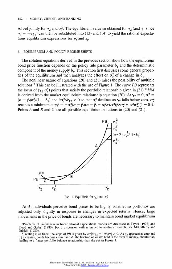
The nonlinear nature of equations (20) and (21) raises the possibility of multiple solutions.7 This can be illustrated with the use of Figure 1. The curve PB represents the locus of (^y2,¢52) points that satisfy the portfolio relationship given in (21).8 MM is derived from the market equilibrium relationship equation (20). At 52 = O, C52 =

((x - )crv2/(l - bI) and da5218^y2 > O so that C52 declines as 2 falls below zero. C52

reaches a minimum at 2* =-CV2(-)(-a-tT)/T2(T2ff62 + R2ff2U)( 1-81)-

Points A and B and C are all possible equilibrium solutions to (20) and (21).

PB 2 ,L 2,

/ / (a-,l9) (r2/(1-8 )

/T s" A /

M M PB B

r2 r2+ r2

FIG. 1. Equilibria for 2 and C2

At A individuals perceive bond prices to be highly volatile, so portfolios are adjusted only slightly in response to changes in expected returns. Hence, large movements in the price of bonds are necessary to maintain bond market equilibrium

7Problems of uniqueness in linear rational expectations models are discussed in Taylor (1977) and Flood and Garber (1980). For a discussion with reference to nonlinear models, see McCafferty and Driskill (1980).

8Treating m as fixed, the slope of PB is given by 8C521872 = l/mp; > 0. As 2 approaches zero and vs2 increases, bonds become riskier and m, the fraction of wealth held 1n the form of money, should rise, leading to a flatter portfolio balance relationship than the PB in Figure l.



CARL E. WALSH : 143

in the face of exogenous shocks. This validates investor beliefs about the volatility of bond prices. At C, investors perceive C2 to be small; 72 iS thus large in absolute value as large portfolio shifts are induced by changes in expected returns. This in turn implies that only small movements in (s,-s,) are necessary to maintain market equilibrium so that (72 will, in fact, turn out to be small. Point B represents an intermediate case that is also consistent with a rational expectations equilibrium.

A simple analysis of local stability suggests that PB must cross MM from below as 72 increases for the equilibrium to be stable. For example, in Figure 1, if individuals initially believe the variance of bond prices is C2', 72 will equal 72 and the actual variance of bond prices will be C2" < C2'. As this becomes perceived, 72

will fall, moving both 72 and C2 toward the equilibrium at point A. By a similar argument, it follows that B is an unstable equilibrium. If the economy were characterized by point B, any slight deviation away from B would move the economy toward either A or C.

Restricting the discussion to stable equilibria eliminates point B, but leaves both A and C as potential equilibria. However, there are two reasons to suggest that point A is the most relevant equilibrium point.9 First, from equation (20), along MM

d(X2 2T2(X2(J2 +(x2(r2)y2 + 2(R a RIXT) s, (22)

where the first term is negative, the second positive. Consider the relationship between 72 and C2 when y, and p, are held constant so that v, represents the only disturbance to the money market. In this case, 8C2/a^Y2 > 0. Hence, the possibility that 8C2/a^Y2 might be negative arises from the indirect effects on the money market of disturbances to aggregate demand or supply. Assuming direct effects dominate would imply that the relevant equilibrium is at a point such as A, where the slope of MM given by (22) is positive, rather than at C where MM is negatively sloped.

Second, the equilibrium at C would imply a relatively large negative value for 72.

Empirical evidence, though, suggests that the interest elasticity of the demand for money is quite small (see Goldfeld 1973). This also would indicate that point A is the most relevant equilibrium point. However, while stability analysis provides a rationale for eliminating point B, the model itself does not allow a choice to be made between A and C.

Equations (20) and (21) can be used to investigate the effects of a monetary policy regime shift, represented here by a change in 81. Assume initially that the economy is in an equilibrium10 characterized by a large, negative value of 81; the monetary authority attempts to offset deviations of s, from s, by engaging in open

9The possibility of an equilibrium point such as C is due to the wealth effect on money demand and the assumption that the policymakers respond to (s, - s,) and not directly to , or u,. In the absence of these two factors, it can be shown that the first term in (20) does not depend on 72. This, in turn, implies that 8as21872 > O everywhere along MM.

I°Equilibrium here means a pair of equations such as (13) and (14) for p, and s,. Prices will not be constant in equilibrium and will deviate from deterministic paths as a result of nonzero realizations of the random disturbances ,, u,, and v,.




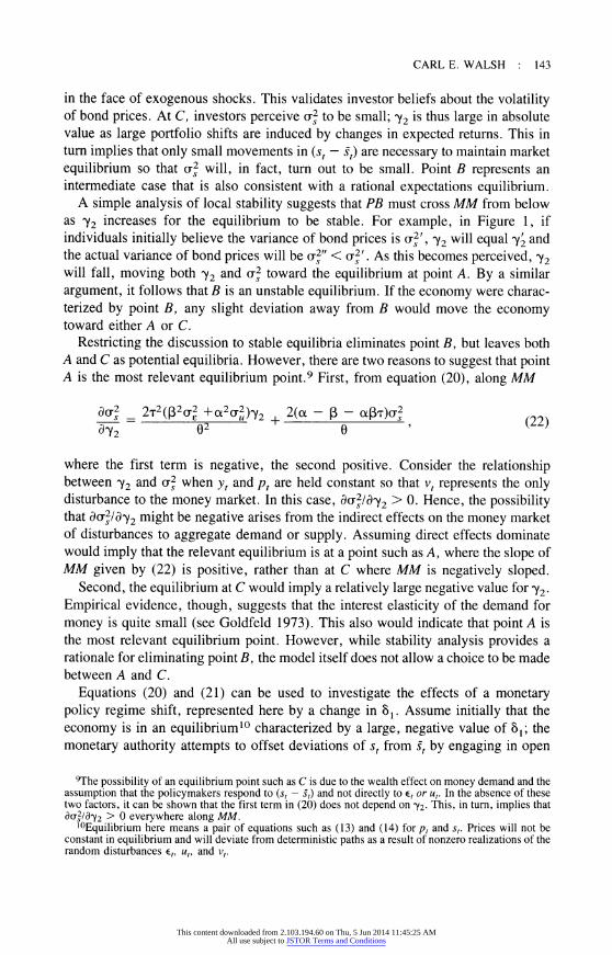
market operations. If bond prices rise above s,, mt is reduced in an attempt to put downward pressure on s,. Let the market equilibrium relationship between 2 and (752 be given by MM in Figure 2; equilibrium is at 72 and C52 (point A).

Suppose that the monetary authority now shifts to a policy associated with a smaller negative value for bl, say 81 with 81 < 81 < 0. From equation (20), for a given 72, 8C521881 = 2(a-) a52/0 > O SO that the new policy results in an upward shift in the MM schedule to MM' in Figure 2. Since the PB schedule given by equation (21 ) is not directly affected by bl, it does not shift. l l The new equilibrium

. .

1S at poznt B. T le policy change results in a new equilibrium in which bond prices are more volatile and the interest elasticity of the demand for money is lower. 12

PB 2 / s

,s,,2k (= a, av ,(I sI,

MM / / (a :)<rV/(I 81)

A - 2

s MM /

PB- --

r2 r-2 r2

FIG. 2. Effect of a Policy shift

Using (20) and (21), the rise in (J52 due to a small rise in 81 is given by

d(r521dbl = 2C4(a- )1(-7205)S (23)

here iv = (_<J2/) ) - 2(T2(l32(J2 + O.2CrU2)72/02 + ((X - ( - cxg8T)(T210) equals the slope of the PB schedule minus that of MM. The assumption of stability, which

requires PB to cut MM from below as PY2 °, implies that /\ > 0. Similarly,

dz21db = 2fr2((x-)10/ > O (24)

In the standard analysis of alternative monetary policy rules (e.g., Poole 1970, Friedman 1977, and McCallum and Hoehn 1983), a shift away from an interest rate

llIf the rise in a2 associated with the upward shift in MM tended to produce an increase in m, PB would shift to the right, reinforcing the effects discussed in the text.

l2If the initial equilibrium had been at a point such as C in Figure 1, the upward shift in MM induced by the policy change would similarly have resulted in a fall in the interest elasticity of the demand for money.



CARL E. WALSH : 145

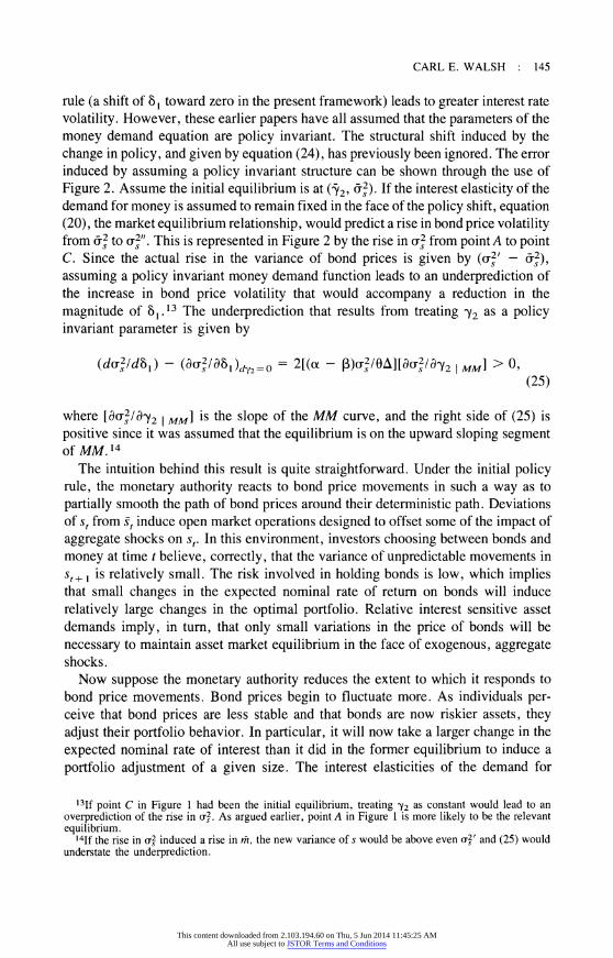
rule (a shift °f 8 1 toward zero in the present framework) leads to greater interest rate volatility. However, these earlier papers have all assumed that the parameters of the money demand equation are policy invariant. The structural shift induced by the change in policy, and given by equation (24), has previously been ignored. The error induced by assuming a policy invariant structure can be shown through the use of Figure 2. Assume the initial equilibrium is at (^Y2, CJ2) If the interest elasticity of the demand for money is assumed to remain fixed in the face of the policy shift, equation (20), the market equilibrium relationship, would predict a rise in bond price volatility from (T2 to cr2". This is represented in Figure 2 by the rise in a2 from pointA to point C. Since the actual rise in the variance of bond prices is given by (cr2' -(r2),

assuming a policy invariant money demand function leads to an underprediction of the increase in bond price volatility that would accompany a reduction in the magnitude of 81.13 The underprediction that results from treating zY2 as a policy invariant parameter is given by

(da51dbl) (acs/abl)dy2=o 2[(t )sl05][8Csl8w2 | MM] > ° (25)

where [8C2/8w2 g MM] iS the slope of the MM curve, and the right side of (25) is positive since it was assumed that the equilibrium is on the upward sloping segment of A8M. 14

The intuition behind this result is quite straightforward. Under the initial policy rule, the monetary authority reacts to bond price movements in such a way as to partially smooth the path of bond prices around their deterministic path. Deviations of s, from s, induce open market operations designed to offset some of the impact of aggregate shocks on s,. In this environment, investors choosing between bonds and money at time t believe, correctly, that the variance of unpredictable movements in 5.+1 is relatively small. The risk involved in holding bonds is low, which implies that small changes in the expected nominal rate of return on bonds will induce relatively large changes in the optimal portfolio. Relative interest sensitive asset demands imply, in turn, that only small variations in the price of bonds will be necessary to maintain asset market equilibrium in the face of exogenous, aggregate shocks.

Now suppose the monetary authority reduces the extent to which it responds to bond price movements. Bond prices begin to fluctuate more. As individuals perceive that bond prices are less stable and that bonds are now riskier assets, they adjust their portfolio behavior. In particular, it will now take a larger change in the expected nominal rate of interest than it did in the former equilibrium to induce a portfolio adjustment of a given size. The interest elasticities of the demand for

13If point C in Figure 1 had been the initial equilibrium, treating Y2 as constant would lead to an overprediction of the rise in a2. As argued earlier, point A in Figure 1 is more likely to be the relevant equilibrium.

14If the rise in 2 induced a rise in m, the new variance of s would be above even C2' and (25) would understate the underprediction.




money and the demand for bonds decline. With 72 now closer to zero, larger bond price movements are required to maintain asset market equilibrium. This implies that the policy shift will produce a larger rise in bond price volatility than would have been the case if there had been no induced structural shift.

One can also employ the model to examine the effect of a policy shift on the volatility of the nominal money supply. From equation (10),

Cm = ^ 12ff52 + Cv2 . (26)

Clearly, if the policy shift is described by a move from a nonzero 81 to 81 = °, am will fall. However, Poole (1982) has argued that after the Federal Reserve's Octo- ber 6, 1979, change in operating procedures, attention was still directed toward reducing interest rate fluctuations. Consider then not a change from a negative to a zero value for 81, but a small reduction in the absolute value of 81 when the initial policy involved a significant, negative 81. Ignoring the induced effect on 72,

(8Cm/88l)dv2=o = 281ff52(1 + 81(st - )/0) < O. (27)

This would be the standard result; if the monetary authority pays less attention to interest rates, the money supply should be less volatile. Recognizing the dependency of structure on policy, however, reveals that

damldbl = 2alaS2(l - al(cx - 13)s215t202\)

(8Cml88l)dy2=o + 2812[(cx - |3)C2/(0/\)][49C2/4905t ]

> (aam/ 88 1 )dy2 = o S (28)

where the inequality follows since from (25) the second term in (28) is positive. The structural shift reduces the fall in am which would be produced by a small movement in 8 1 toward zero. If 81 < ° and 7205 - 81 (t - )C52 > O, then damldb 1 > ° A movement away from an interest rate policy, in this case, actually leads to an increase in the variance of the nominal money supply. Even though m is adjusted less in response to any given movement in (s, - s,), the induced rise in the variance of (s, - s,) causes the nominal money supply to become more volatile.

The specific expressions derived in equations (25) and (28) depend, of course, on the particular formulation of the portfolio choice problem in section 2 used to interpret the parameters of the money demand function. However, the basic result is more general than might be suggested by a model that derives a money demand equation within an asset demand, rather than inventory theoretic, framework. As shown by Buiter and Armstrong (1978) and Niehans (1978), if interest rates are stochastic, a Baumol-Tobin inventory approach to the demand for money also implies that the interest elasticity of the demand for money is a function of the stochastic properties of the rate of interest. A shift in monetary policy that alters the



CARL E. WALSH : 147

behavior of interest rates will induce changes in the parameters characterizing money demand. Such parameter shifts, in turn, further affect the stochastic behavior of interest rates.

5. OPTIMAL POLICY

While the focus of this paper has been on the structural shifts induced by a change in the monetary authority's policy rule, the model can also be used to study the issue of optimal policy. This section looks briefly at the implications of the analysis for the choice of 81 if the monetary authority's objective is to minimize the variance of real output around trend.15

From (1 ) and (2) it follows that the unconditional expected values of Yt and (St+ 1

- Pt+ 1) will be independent of the monetary policy rule. Using ( 16), or (2), the average real rate of interest will be nl ,82. The average nominal rate of return, St + 1

s,, however, will be equal to k, the growth rate of the deterministic component of the money supply. In an equilibrium with y, = y,, the fraction of wealth held as money is constant. Since the number of bonds outstanding is also constant, bond prices must rise at the same rate as the money supply in order to maintain constant portfolio shares. As shown by ( 18), the aggregate price level rises at a constant rate less than k.

Because aggregate supply is assumed to depend on (p,-,_ IP.) and the monetary policy rule allows m, to respond to the contemporaneous price of bonds, the behavior of y,-y, will be influenced by the choice of 81. Using (1) and (13),

yt = yr + (1 -PY2-aI)(tut-Et)le-avtlO , (29)

where oY2 iS obtained as the solution to (20) and (21). The variance of Yt-Y-t, the deviation of real output from trend, is

(Jy2 = (1 -tY2-al)2(cx2Cr2 + 2C2)102 + Cx2f32fr2l>2 (30)

This variance is a function of the policy parameter 81 both directly and through the dependence °f PY2 on 81 * If wY2 iS treated as a constant, the value of 81 that minimizes ay2 iS given by

1 1 Y2 cx 13(Ct - |3)crV2/Tty2(cx2(T2 + 2fJ2) (31 )

This value is found by setting 8(xy218bl equal to zero, where the partial derivative notation signifies Y2 iS being held constant.

That is, optimal policy, given the policy rule (10), is examined. l6It is interesting to note that choosing 81 = 1 -Y2 automatically insulates y,-y, from aggregate

supply and demand shocks. In this case, (29) reduces to y,-y, + (mpcS2)v,. An increase in bond price volatility makes output more sensitive to nominal money supply shocks.




When it is recognized that 72 iS a function °f 81, the first-order condition for the minimization Of a2 with respect to 81 is

d,T2/dbl = 8fx2/ab1 + (da2l8^y2)(dty2ldbl) = ° (32)

At 81*, ACx2/a^Y2 =-2cx,(3Xa2/0 which is positive. From (24), da21dbl > O. There- fore, at 81*

da21dbl = (dC2l872)(d72ldal) > ° ( )

By the second-order condition for a minimum, 82C2/a82 > 0 at 81*. Hence, (32) and (33) taken together imply that, if 81** satisfies (32), 81* > 81**. Ignoring the dependence of 72 on 81 leads to a choice °f 81 that is too large. Since, from (23), da2ldbl > O, the choice of 81* by the monetary authority leads to more bond price volatility than would occur at the optimal 81**.

Another way of stating this result is the following: if the parameters of the portfolio balance equation are treated as policy invariant, the monetary authority will choose a value of 81 to minimize a2, which leads to more bond price volatility and less money supply volatilityl7 than would occur at the true optimum given by 81**

6 SUMMARY AND CONCLUSIONS

Using a fairly conventional rational expectations aggregate model, it has been shown how the coefficients in the portfolio balance, or money demand, equation are functions of the stochastic behavior of bond prices. Since the behavior of the price of bonds is itself dependent upon the monetary authority's actions, changes in policy result in shifts in the interest and income elasticities of the demand for money. Such structural shifts induce further changes in the equilibrium relationship between bond prices and the exogenous random disturbances in the model. The model suggests that a shift toward a policy that allows for greater fluctuations in the price of bonds, as, for example, occurs if the monetary authority changes from an interest rate to a reserve aggregate operating procedure, may result in a larger increase in bond price volatility than would have been predicted under the assumption of a constant structure. This is an example of the relevance of the Lucas policy evaluation critique to the problem of evaluating the implications of alternative monetary policy operating procedures.

The monetary policy rule plays an important role in affecting investor decisions because real returns are random. Consequently, to evaluate the relative real returns on bonds and money requires knowledge of how the money supply will be adjusted in the future to what are currently unobserved events. In the present model, returns

17This assumes da2 /dbl < O. See equation (28).



CARL E. WALSH ; 149

depend on future shocks to which monetary policy will respond. Similar results obtain if current shocks are imperfectly observed and the future money supply will be adjusted when current shocks become observable (see Weiss 1980 and King 1982).

Since Poole's classic paper (Poole 1970), it has been common to employ simple aggregate models to analyze the implications of alternative monetary policy Iules. These models assume that behavioral relationships are policy invariant. 18 Because the stochastic behavior of asset returns is likely to depend on the process governing the money supply, asset demand functions as normally specified will not satisfy this policy invariance assumption. A complete analysis of alternative monetary policy rules must allow for this dependence of stimcture on policy.

LITERATURE CITED

Aoki, Masanao, and Matthew B. Canzoneri. "Reduced Forms of Rational Expectations Models. " Quarterly Journal of Economics 93 (February 1979), 59-71.

Boonekamp, Clemens F. J. "Inflation, Hedging, and the Demand for Money." American Economic Review 68 (December 1978), 821-33.

Bryant, John, and Neil Wallace. "A Suggestion for Further Simplifying the Theory of Money." Staff Report 62, Federal Reserve Bank of Minneapolis, August 1980.

Buiter, Willem H., and Clive A. Armstrong. "A Didactic Note on the Transactions Demand for Money and Behavior Towards Risk." Journal of Money, Credit, and Banking 10 (November 1978), 529-38.

Eaton, Jonathan, and Stephen J. Turnovsky. "Exchange Risk, Political Risk, and Macro- economic Equilibrium." American Economic Review 73 (March 1983), 183-89.

Fair, Ray C. "Estimated Effects of the October 1979 Change in Monetary Policy on the 1980 Economy." Papers and Proceedings of the American Economic Association 71 (May 1981), 160-65.

Feige, Edgar L., and Robert McGee. "Has the Federal Reserve Shifted from a Policy of Interest Rate Targets to a Policy of Monetary Aggregate Targets?" Journal of Money, Credit, andBanking 11 (November 1979), 381-404.

Fischer, Stanley. "Long-Term Contracts, Rational Expectations, and the Optimal Money Supply Rule. " Journal of Political Economy 85 (February 1977), 191 -205.

Flood, Robert P., and Peter M. Garber. "Market Fundamentals versus Price Level Bubbles: The First Tests. " Journal of Political Economy 88 (August 1980), 745-70.

Friedman, Benjamin M. "The Inefficiency of Short-Run Monetary Targets and Monetary Policy." Brookings Papers on Economic Activity 2 (1977), 293-335.

Goldfeld, Stephen M. "The Demand for Money Revisited." Brookings Papers on Economic Activity 3 (1973), 577-638.

King, Robert G. "Monetary Policy and the Information Content of Prices." Journal of Political Economy 90 (April 1982), 247-79.

Klein, Benjamin M. "The Demand for Quality-Adjusted Cash Balances: Price Uncertainty in the U .S . Demand for Money Function. " Journal of Political Economy 85 (August 1977), 691-715.

l8Bryant and Wallace (1980) characterize this as the "starting from curves" approach to macroeconomics .




Lucas, Robert E., Jr. "Econometric Policy Evaluation: A Critique." In The Phillips Curve and Labor Markets, edited by Karl Brunner and Allan H. Meltzer, pp. 19-46. The Carnegie-Rochester Conferences Series, Vol. 1. Amsterdam: North-Holland, 1976.

. "Asset Prices in an Exchange Economy." Econometrica 46 (November 1978), 1429-45.

McCafferty, Stephen A., and Robert A. Driskill. "Problems of Existence and Uniqueness in Non-Linear Models of Rational Expectations. " Econometrica 48 (July 1980), 1313-17.

McCallum, Bennett T. "Rational Expectations and Macroeconomic Stabilization Policy: An Overview." Journal of Money, Credat, and Banking 12 (November 1980, pt. 2), 716-46.

. "Price Level Determinacy with an Interest Rate Policy Rule and Rational Expecta- tions." Journal of Monetary Economics 8 (November 1981), 319-29.

McCallum, Bennett T., and James G. Hoehn. "Instrument Choice for Money Stock Control with Contemporaneous and Lagged Reserve Requirements." Journal of Money, Credit, and Banking 15 (February 1983), 96-101.

McCallum, Bennett T., and John K. Whitaker. "The Effectiveness of Fiscal Feedback Rules and Automatic Stabilizers under Rational Expectations." Journal of Monetary Economics 5 (April 1979), 171-86.

Niehans, Jurg. The Theory of Money. Baltimore: Johns Hopkins University Press, 1978.

Poole, William. "Optimal Choice of Monetary Policy Instruments in a Simple Stochastic Macro Model." Quarterly Journal of Economics 84 (May 1970), 197-216.

. "Federal Reserve Operating Procedures: A Survey and Evaluation of the Historical Record since October 1979." Journal of Money, Credit, and Banking 14 (November 1982, pt. 2), 575-96.

Santomero, Anthony M., and John J. Seater. "Partial Adjustment in the Demand for Money: Theory and Empirics." American Economic Review 71 (September 1981), 566-78.

Sargent, Thomas J., and Neil Wallace. "'Rational' Expectations, the Optimal Monetary Instrument, and the Optimal Money Supply Rule." Journal of Political Economy 83 (April 1975), 241-54.

Taylor, John B. "Monetary Policy During a Transition to Rational Expectations." Journal of Political Economy 83 (October 1975), 1009-21.

. "Conditions for Unique Solutions in Stochastic Macroeconomic Models with Ra- tional Expectations." Econometrica 45 (September 1977), 1377-86.

Tinsley, Peter A., Peter von zur Muehlen, Warren Trepeta, and Gerhard Fries. "Money Market Impacts of Alternative Operating Procedures." In Federal Reserve Staff Study, New Monetary Control Procedures, Vol. 2. Washington, D.C.: Board of Governors of the Federal Reserve System, 1981.

Tobin, James. "Liquidity Preference as Behavior Towards Risk." Review of Economic Studies 25 (February 1958), 65-86.

Walsh, Carl E. "Asset Prices, Asset Stocks, and Rational Expectations." Journal of Mone- tary Economics 11 (May 1983), 337-49.

Weiss, Laurence. "The Role for Active Monetary Policy in a Rational Expectations Model." Journal of Political Economy 88 (April 1980), 221-33.

Woglom, Geoffrey. "Rational Expectations and Monetary Policy in a Simple Mac- roeconomic Model." Quarterly Journal of Economics 93 (February 1979), 91-105.



interest rate volatility and monetary policy

Documents