Interconnection Negotiations between Telecommunication

Networks and Universal Service Objectives

Vasiliki Skreta∗

University of Minnesota

skreta@econ.umn.edu

March 2004

Abstract

We study negotiations between Telecommunication Networks over access fees, that is, fees one net-

work has to pay to another one, whenever a customer of the former places a phone call to a customer

of the latter. We show that revenue generated from agreed access fees can alleviate the problem of

providing telecommunication services at reasonable prices at rural and other high cost areas. The model

consists of three interconnected networks - two located in the low cost area (urban area) and one located

in the high cost (rural area) - who negotiate pair-wise over access fees. If urban customers place high

value to being able to reach rural customers, then the rural network’s revenue from selling access will

be high enough so that it will become profitable given interconnection, even though it would be making

losses if it were not interconnected with the urban networks. The reason is that access fees allow market

participants to internalize some of the network externalities. The results are robust with respect to the

timing of the moves of the game and, more importantly, with respect to the degree of competition in

the urban market. The lessons apply to other industries that have the network structure, for instance

electricity, postal services and transportation.

∗This work is included in Chapter 3 of my doctoral thesis submitted to the Faculty of Arts and Sciences at the University of

Pittsburgh. I would like to thank Mark Armstrong, Jim Dana and Esther Gal-Or for very helpful comments and discussions.

I would also like to thank the Department of Management and Strategy, KGSM, Northwestern University for its warm

hospitality, the Andrew Mellon Pre-Doctoral Fellowship, the Faculty of Arts and Sciences at the University of Pittsburgh and

the TMR Network Contract ERBFMRXCT980203 for financial support. All remaining errors are of course mine. Preliminary

version.

1

1 Introduction

This paper addresses the issue of providing universal service in a deregulated network. Many industries

that have a network structure, for instance gas, electricity, telecommunications and postal services, exhibit

large cost discrepancies. The provision of the ‘same’ service may cost as much as ten times more in some

parts of the network than in others. When this is the case, it is profitable to operate only in some areas. In

most countries, till relatively recently, these industries were either state-owned monopolies or regulated by

the government. Under these ownership structures the government was able to cross-subsidize high-cost

with low-cost, profitable areas.1 Currently the markets for telecommunications services, gas and electricity

in the United States, and in other countries are undergoing major changes. Most of the firms operating

in these industries have been privatized and regulation is being replaced by competition. As many have

observed, see for instance Baumol (1999), direct cross-subsidies may be incompatible with competition and

deregulation.

The objective of this paper is to demonstrate how indirect cross-subsidization can take place in a dereg-

ulated environment. More specifically, we would like to identify market conditions that ensure universal

coverage of telecommunication services without government subsidies. Most of the analysis will be based

on the telecommunication industry, but a lot of the insights obtained carry over to other industries as well.

After the introduction of the Telecommunications Act of 1996 by the Congress, the market for local

and long distance service is opened to competition. The major technological breakthroughs in the telecom-

munication and other related industries changed the structure of the telecommunication markets. Due to

these technological advances the distinction between telecommunication and information services, such as

access to the information superhighways, became unclear. This created the need to change the institutions

that govern telecommunication markets in order to avoid creating distortions. According to the previous

arrangement the provision of local telephone services was delivered by local monopolies, the Regional Bell

Operating Companies, (RBOCs), which were subject to regulation. On the other hand, the markets for long

distance services and for internet access were open to competition. The Congress in order to accommodate

the technological advancements passed the Telecommunications Act of 1996 which opened all telecommu-

nication markets to competition. This Act contains a clause that states that advanced telecommunication

and information services must be available to all Americans at reasonable rates. This clause is included

into what the Federal Communication Commission, FCC, refers to as ‘universal service objectives,’ USOs.

The fact that there exist big cost discrepancies in providing telecommunication services in different

areas, has lead many to believe that deregulation will threaten universal service objectives. One would

1See Maria Maher (1999) for an empirical study which shows that there are economies of scale in the provision of access

to the local telecommunication network and that costs differ by geographical location.

2

expect that no firm will be willing to provide services in high cost areas, such as remote and sparsely

populated rural areas, whereas competition will prevail in densely populated and more profitable urban

areas. Under the previous arrangement the prices charged by the regulated RBOC reflected a cross sub-

sidy from urban to rural markets. This kind of direct cross subsidization is likely to be impossible in a

deregulated environment. The Congress realizing this problem asked the FCC to form a Federal-State

Joint Board to specify the services that should be included in the universal service objectives and ways to

financially support them, [16]. Similar documents have been prepared by Oftel, [25], in the UK and by the

European Commission, [15], among many others. The major priority of the universal service objectives

is the provision of advanced telecommunication and information services to rural customers at prices that

are comparable to the ones that urban customers pay.

The goal of this research is to show that this objective can be achieved without outside subsidies in

a deregulated2 market of telecommunication services. The reason is positive network externalities. The

value generated from serving a rural customer does not only include his willingness to pay for telephone

service, but also the utility that other customers enjoy from being able to reach him. If urban customers,

residential and businesses, like to place many phone calls in the rural market, then the urban networks

may find it profitable to subsidize the rural ones. Providing service to rural customers increases the profits

of a network serving an urban area, since urban customers can place more phone calls. Interconnection

enlarges the market and the benefit of having more customers connected accrues to all parts of the network.

Similar observations hold for other industries, for instance postal services. Delivering a letter to a relative

in a remote area generates surplus to the receiver as well as to the sender.

Our model consists of two different markets; a rural or high cost area and an urban or low cost area.

There is only one network operating in the rural market. In the urban market we consider three alternative

scenarios. First we look at the case there is only one urban network, (monopoly), and then we consider the

case of a competitive urban market, and finally the more realistic case, where there are two horizontally

differentiated urban networks. We assume that networks choose their prices non-cooperatively and they

bargain pairwise over the level of access fees. The outcome of negotiations is determined by the Nash-

Bargaining solution. We demonstrate that interconnection is a feature of the market that may support

universal service, even in a deregulated market.3 How? The rural network generates revenue by selling

services to rural customers AND by selling access to its facilities to the urban networks. Urban networks

pay an access fee to the rural network each time an urban customer places a call to a rural customer (and

the opposite). Under certain conditions net access revenue of a rural network can lead to positive profits,

even if this network would make losses if it were isolated (that is, in the case that there were no calls made

2For an excellent survey of the enormous literature on regulation see Armstrong and Sappington (2004).3 ‘Interconnection’ means that customers of one network can reach customers of the other network.

3

between urban and rural customers).

When we examine the case of horizontally differentiated urban networks, our model builds on Armstrong

(1998), Carter and Wright (1999), and Laffont, Rey and Tirole (1998a). These papers study, among others,

competition between telecommunication networks in a deregulated or partially regulated environment.

Their focus is on the determination of the price of telecommunications services and of the access fees that

each network pays to competing networks, when a customer of the former places a call to a customer

of the latter. We extend the basic model by studying the determination of access fees and prices in an

environment that consists of three interconnected networks. There is two-way access between all networks

and competition for customers between the networks located in the urban area. This model has the

advantage that it builds upon the standard network-interconnection model - which makes our analysis

directly comparable to the existing ones; the downside is that it does not allow for tractable analytical

results. We calculate the equilibrium prices and access fees in a parametrized example and show that in

many instances, even though the rural network would be making losses if it were not interconnected with

the urban networks, it will become profitable if there is interconnection. The urban network subsidizes

the rural network in the following way: whenever a rural customer places a call to an urban customer the

urban network charges a negative access fee to the rural network. This result is robust to different sequence

of moves of the game.

Our results demonstrate that if urban customers place a large enough fraction of their total demand for

calls to rural customers, then the rural network generates revenue from selling access that is high enough

to cover its losses from providing telecommunication services. If this is the case in some markets, then

there is no need to arrange for outside subsidies, since the market is viable on its own. One would think

that such an insight that is based on ‘voluntary’ cross subsidization, between the urban and the rural

market, would be vulnerable to the degree of competition in the urban market, the argument being that

competition erodes profits, and there is nothing left for ‘cross-subsidization.’ Our results suggest that this

is not true at least in the case where there is only one network serving the rural area, (which given large

fixed costs is probably the scenario that is most likely). Actually it is exactly the opposite. The monopoly

power of the rural network vis-a-vis urban networks that offer indistinguishable services, and hence have no

market power, makes it a very tough negotiator. When the rural network bargains with an urban network

over access fees, the rural network knows that if they fail to reach agreement, the urban network will suffer

a severe loss in market share, (in the extreme case we solved analytically it will be actually kicked out of

the market). The reason being that no urban customer would like to pay the same price for telephone

service and not being able to complete phone calls across markets, when he/she can buy service from some

other network that has interconnection with the rural market. On the other hand, the rural network does

not loose anything in the event that it fails to reach agreement with a particular urban network, since it

4

can still connect with the other urban networks who now serve all the market. This mechanism, that is

the effect of interconnection agreements on market shares, is also present in the case that urban networks

have some market power, but is less extreme. In those cases though there is different channel for potential

allowing sufficient subsidizations: the higher the market power the higher the profits of urban networks.

But higher market power also means higher bargaining power vis-a-vis the rural network, that is higher

market power in the urban market implies higher profits but also stronger bargaining position, whereas

low market power implies very low profits in the urban market but at the same time, very weak position in

the negotiations. In other words depending on the market power in the urban market there are different

mechanisms in place that work in favor of cross-subsidization. A weakness of the current analysis is that

our results are completely silent to whether prices will be comparable across markets. In the future we

plan to investigate the effect of cross-market price constraints, similar to the ones in [1], on the negotiated

access fees and on the equilibrium profits.

There has been some recent theoretical work that studies universal service objectives issues but with

different focus then the current project. Anton, Weide and Vettas (2002) develop a multi-market model

that consists of an oligopolistic urban market, entry auctions for rural service and cross market price

restrictions. They analyze how these restrictions affect pricing in the urban market and entry decisions

in the rural market. The assumed market structure does not consist of networks so there is no other

interconnection between the rural and the urban market. Laffont and Tirole (2000) in Chapter 6 discuss

Universal Service Obligations. They offer some institutional background and analyze ways to generate the

“right subsidies” by means of designing auction mechanisms that determine, among, others the structure of

the market, (auction mechanisms with endogenous market structure). Milgrom (1996) is the first to discuss

the application of mechanisms with endogenous market structure, developed by Dana and Spier (1994),

in Universal Service Obligations.4 Compared to the previous work, our focus is not how to generate the

right subsidies for USOs, but to demonstrate that outside intervention and subsidies may not be necessary.

Baumol (1999) and Armstrong (2001a), like this paper, are concerned with the issue of how competition

will affect USO’s. Both consider the stage of transition to competition, where there is an incumbent

network who faces potential entrants that may or may not bypass its facilities. The incumbent does not

need to buy access to the entrant’s facilities. The focus of those papers is to determine the access fees

paid to the incumbent by the entrant that generate efficient entry, and when bypass is possible, efficient

make-or-buy decisions for the entrant. Here we examine the case of mature competition where all networks

need to purchase necessary inputs from each other. The papers by Riordan (2000) and (2001) investigate

the economic rational for USO’s. In this paper we do not aim at exploring whether USO’s is indeed an

4See also Weller (1998).

5

appropriate objective, but we show that it can be achieved even in a deregulated environment.

2 Unit Demands

2.1 Monopoly in the Urban Market

2.1.1 The model

We will start by examining a very simple scenario. We consider a situation where there are two telecom-

munication networks, A and R. Network A operates in the low cost area (or urban area) . Network R

is located in the high cost area, the rural area. When a subscriber of A calls a subscriber of R, A has

to ‘buy’ access to R’s subscribers. In short, network i sells access to network j and the opposite. Hence

there is ‘two-way’ access without competition between network R and network i = A,B. In order for urban

customers to be able to terminate a call in the rural market, and the reverse, the urban and the rural

network must sign an interconnection agreement.

• Demand Structure in the Urban Market

We assume that

• consumers derive utility only from placing and not from receiving phone calls.

The utility of an urban consumer connected to network A is given by

U(pA) = v − pA.

In the rural market there is a single network called R. The net surplus for a rural customer from being

connected to the network is given by

U(pR) = v − pR.

We consider the case where demand for phone calls in both markets is fixed and equal to one. A rural

customer places a fraction rR of the total calls within the rural market and a fraction (1−rR) to the urbanmarket. Similarly, an urban customer places a fraction rU of the total calls within the urban market and a

fraction (1−rU ) to the rural market. A result of this assumption is that the demand of network A dependson whether it has signed an interconnection agreement with R.

In the case that A signs interconnection agreements with R, its demand is given by

dA(pA) =

(1 if v − pA ≥ 00 otherwise

,

6

where pA stands for the price charged by A in case it has signed an interconnection agreement with R. In

case of disagreement with R demand is given by

dDA (pDA ) =

(ru if v − pDA ≥ 00 otherwise

,

where pDA denotes the price charged by A in case it fails to sign an interconnection agreement with R.

Similarly, in case of agreement with A, the demand for the rural network is given by

dR(pR) =

(γ if v − pR ≥ 00 otherwise

,

where γ ∈ [0, 1] and pR stands for the price that the rural network charges in case of agreement with A.

Let pDR denote the price charged by the rural network in case of disagreement with A. In this event, the

demand of the rural network is given by

dDR(pDR) =

(γrR if v − pDR ≥ 00 otherwise

.

• Cost Structure and Profits

Now we specify the cost structure of the networks. Let5 coi denote the cost of originating a phone call

from network i, and cTi the cost of terminating a phone call at network i, i = A,R. Network i incurs a

fixed cost cFi of servicing a customer.

We use pi to denote the price set by network i and tAR , (tRA), to denote the access fee that the rural

network R, (A), pays to network A, (R), each time a subscriber of network R, (A), calls a subscriber of

network A, (R).

Remark: We will argue in a minute that networks will not charge different prices for phone calls completed

within the network and phone calls completed across networks.

Given this observation network A0s and R0s profits are given by

ΠA = pA − c0A − rUcTA − (1− rR)c

TA − (1− rU )tRA + (1− rR)γtAR − cFA

ΠR = γ(pR − c0R)− rRγcTR − (1− rU )c

TR − (1− rR)γtAR + (1− rU )tRA − cFR

Let

πA(p) =¡p− coA − cTA

¢, and

πR(p) =¡p− coR − cTR

¢,

5The cost structure is similar to the one in Armstrong (1998).

7

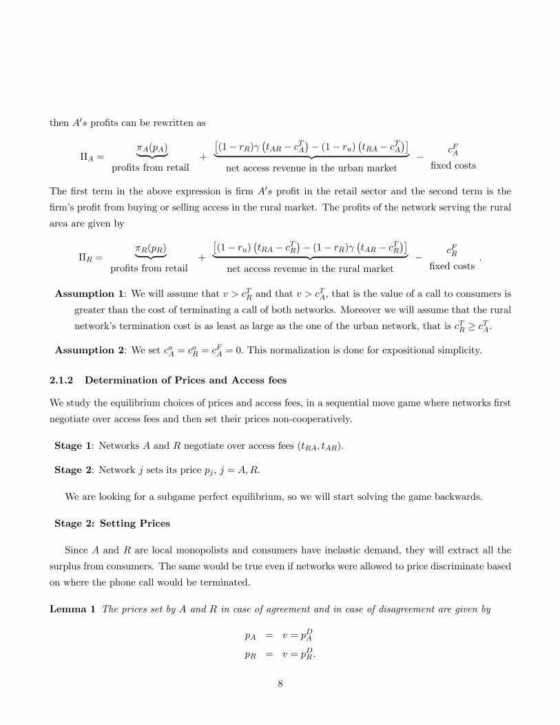
then A0s profits can be rewritten as

ΠA =πA(pA)| {z }

profits from retail+

£(1− rR)γ

¡tAR − cTA

¢− (1− ru)¡tRA − cTA

¢¤| {z }net access revenue in the urban market

− cFA

fixed costs

The first term in the above expression is firm A0s profit in the retail sector and the second term is the

firm’s profit from buying or selling access in the rural market. The profits of the network serving the rural

area are given by

ΠR =πR(pR)| {z }

profits from retail+

£(1− ru)

¡tRA − cTR

¢− (1− rR)γ¡tAR − cTR

¢¤| {z }net access revenue in the rural market

− cFR

fixed costs.

Assumption 1: We will assume that v > cTR and that v > cTA, that is the value of a call to consumers is

greater than the cost of terminating a call of both networks. Moreover we will assume that the rural

network’s termination cost is as least as large as the one of the urban network, that is cTR ≥ cTA.

Assumption 2: We set coA = coR = cFA = 0. This normalization is done for expositional simplicity.

2.1.2 Determination of Prices and Access fees

We study the equilibrium choices of prices and access fees, in a sequential move game where networks first

negotiate over access fees and then set their prices non-cooperatively.

Stage 1: Networks A and R negotiate over access fees (tRA, tAR).

Stage 2: Network j sets its price pj , j = A,R.

We are looking for a subgame perfect equilibrium, so we will start solving the game backwards.

Stage 2: Setting Prices

Since A and R are local monopolists and consumers have inelastic demand, they will extract all the

surplus from consumers. The same would be true even if networks were allowed to price discriminate based

on where the phone call would be terminated.

Lemma 1 The prices set by A and R in case of agreement and in case of disagreement are given by

pA = v = pDA

pR = v = pDR .

8

Proof: A and R face no competition. In this unit demand model the networks in both markets set a

price that extracts all consumer surplus, that is

pA = v = pDA

pR = v = pDR ,

where pj , j = A,R is network j0s price in case of agreement and pDj is j0s price in case of disagreement.

Stage 1: Negotiations

We examine the determination of access fees through free negotiations without regulation. Networks will

be assumed to negotiate pairwise over access fees. The outcome of negotiations is determined by the Nash

Bargaining Solution. The US Telecommunication Act of 1996 states that access fees should be negotiated

among networks subject to regulatory approval. In Europe interconnection agreements should be negotiated

within the framework of the European Law and the supervision of the National Regulatory Agencies. In

other countries, for instance in New Zealand, after the privatization of the national telecommunication

provider, there is no regulatory agency and networks should reach interconnection agreements that do not

violate the existing antitrust laws.

The Nash Bargaining solution is a cooperative solution concept, that allows for a parsimonious repre-

sentation of the conflicts of interests in a given negotiation. According to the Nash Bargaining Solution,

negotiating parties split the ‘gains from reaching an agreement’, equally among each other. For a discussion

of the application of the Nash Bargaining Solution to various bargaining problems and its relationship with

non-cooperative dynamic solution concepts see Binmore, Rubinstein and Wolinsky (1986).

The access fees should solve:

(tAR, tRA) ∈ argmax(ΠA −ΠDA )(ΠR −ΠDR). (1)

The payoffs that accrue to A and R respectively in case of agreement are given by

ΠA = (v − cTA)−RAR − [γ(1− rR)− (1− rU )]cTA

and

ΠR = γ(v − cTR)− cFR +RAR + [γ(1− rR)− (1− rU )]cTR

where

RAR = (1− rU )tRA − (1− rR)tARγ.

9

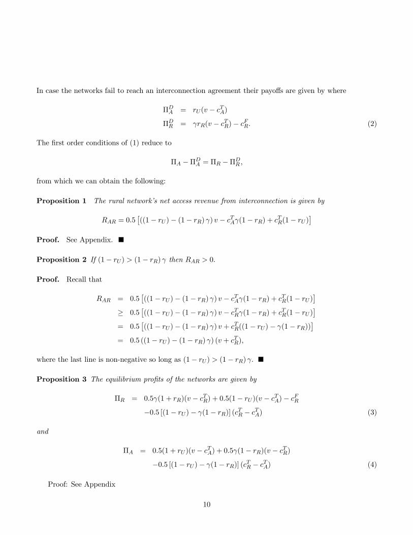
In case the networks fail to reach an interconnection agreement their payoffs are given by where

ΠDA = rU (v − cTA)

ΠDR = γrR(v − cTR)− cFR. (2)

The first order conditions of (1) reduce to

ΠA −ΠDA = ΠR −ΠDR ,

from which we can obtain the following:

Proposition 1 The rural network’s net access revenue from interconnection is given by

RAR = 0.5£((1− rU )− (1− rR) γ) v − cTAγ(1− rR) + cTR(1− rU )

¤Proof. See Appendix.

Proposition 2 If (1− rU ) > (1− rR) γ then RAR > 0.

Proof. Recall that

RAR = 0.5£((1− rU )− (1− rR) γ) v − cTAγ(1− rR) + cTR(1− rU )

¤≥ 0.5

£((1− rU )− (1− rR) γ) v − cTRγ(1− rR) + cTR(1− rU )

¤= 0.5

£((1− rU )− (1− rR) γ) v + cTR((1− rU)− γ(1− rR))

¤= 0.5 ((1− rU )− (1− rR) γ) (v + cTR),

where the last line is non-negative so long as (1− rU ) > (1− rR) γ.

Proposition 3 The equilibrium profits of the networks are given by

ΠR = 0.5γ(1 + rR)(v − cTR) + 0.5(1− rU )(v − cTA)− cFR

−0.5 [(1− rU )− γ(1− rR)] (cTR − cTA) (3)

and

ΠA = 0.5(1 + rU )(v − cTA) + 0.5γ(1− rR)(v − cTR)

−0.5 [(1− rU )− γ(1− rR)] (cTR − cTA) (4)

Proof: See Appendix

10

Remark 1 The rural network’s equilibrium profits will be non-negative provided that

0.5 (γ(1 + rR) + (1− rU )) v

≥ cFR + cTR (γrR + 0.5(1− rU )) + 0.5γ(1− rR)cTA

Remark 2 Both networks benefit from interconnection. From (2) and (3), (4) we obtain that

ΠR −ΠDR = 0.5γ(1− rR)(v − cTA) + 0.5(1− rU )(v − cTR) ≥ 0. (5)

For network A one can obtain

ΠA −ΠDA = 0.5(1− rU )(v − cTA) + 0.5(1− rU )(v − cTR) ≥ 0. (6)

From (5) and (6 we see that both networks benefit from interconnection.

We proceed to examine the effect of parameters on the equilibrium profits of the networks.

Proposition 4 The equilibrium profits of the rural network are (i) decreasing in rU and (ii) increasing in

rR if 0.5v+0.5cTA ≥ cTR. The urban network´s equilibrium profits are (i) increasing in rU and (ii) decreasing

in rR.

Proof. Partially differentiating with respect to the corresponding parameters we obtain

∂ΠR∂rU

= −v0.5− 0.5cTR < 0 since v > cTR

∂ΠR∂rR

= 0.5vγ − cTRγ + 0.5cTAγ ≥ 0

if 0.5v + 0.5cTA ≥ cTR.

and

∂ΠA∂rU

= 0.5v + 0.5cTR − cTA > 0 since v > cTR ≥ cTA

∂ΠA∂rR

= −0.5γv + 0.5γcTA < 0, since v > cTA.

The profits of the rural network are decreasing in rU , where rU stands for the fraction of urban phone

calls completed within the urban market. Also ΠR are increasing in rR so long as the termination costs

11

in the rural network, cTR are not too high. Finally as expected, ΠR is increasing in v and decreasing in cTR

and cFR, that is∂ΠR∂v

> 0,∂ΠR

∂cTR< 0, and

∂ΠR

∂cFR< 0.

Contrary to the rural network, the urban network’s profits are increasing in rU and decreasing in rR. We

will later establish that the qualitative results obtained in this very simple model match the ones we will

obtain when we study via simulations a more elaborate model that was based on the standard 2 - way

network interconnection model.

In this section we looked at a polar case where the urban network is a monopolist in the market. In

order to see whether the obtained results are robust to other market structures, we examine first the case

of a competitive urban market and then the case where networks have some market power.

2.2 Competitive Urban Market

2.2.1 The Model

We examine the scenario where two networks operating in the urban market, call them A and B offer

indistinguishable services. Consumers have inelastic demand for phone calls. We normalize the number of

phone calls demanded by consumers in the urban market to one. A fraction rU of these calls are completed

within the urban market and a fraction (1− rU) are directed to the rural market.

Assumption: Balanced calling pattern: A customer of A calls with equal probability a subscriber of

A and a subscriber of B.

Let s denote A0s market share in the urban market. Networks A and B charge different prices for calls

terminating in different networks. We use pi to denote the price charged by i for calls completed within i;

pji stands for the price charged by i for the calls completed in network j.

Consumer Preferences and Demand

In the urban market consumers may subscribe to just one network. We assume that rU is the fraction

of total phone calls completed within the urban market and (1− rU ) is the percentage of total phone calls

that are directed to the rural market. Consider a consumer subscribing to i, that her indirect utility

ψi(pi, pji , p

Ri ,m) = srU (v − pi) + (1− s)rU(v − pji ) + s(1− rU )(v − pRi ) +m, i, j ∈ {A,B}

where m represents the consumption of other goods. Note that in this model 1 denotes the aggregate

quantity of phone calls that the average subscriber of network i plans to make. Some of these phone calls

are completed within the urban market , whereas some are made to customers in the rural market.

12

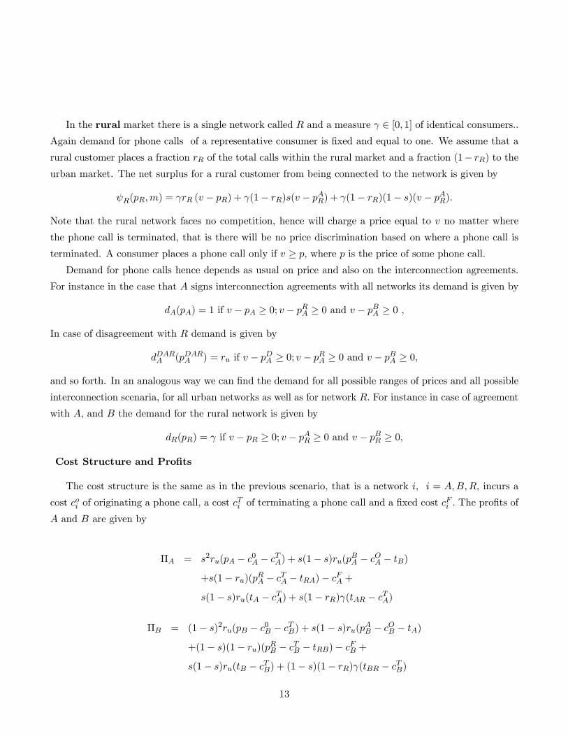
In the rural market there is a single network called R and a measure γ ∈ [0, 1] of identical consumers..Again demand for phone calls of a representative consumer is fixed and equal to one. We assume that a

rural customer places a fraction rR of the total calls within the rural market and a fraction (1− rR) to the

urban market. The net surplus for a rural customer from being connected to the network is given by

ψR(pR,m) = γrR (v − pR) + γ(1− rR)s(v − pAR) + γ(1− rR)(1− s)(v − pAR).

Note that the rural network faces no competition, hence will charge a price equal to v no matter where

the phone call is terminated, that is there will be no price discrimination based on where a phone call is

terminated. A consumer places a phone call only if v ≥ p, where p is the price of some phone call.

Demand for phone calls hence depends as usual on price and also on the interconnection agreements.

For instance in the case that A signs interconnection agreements with all networks its demand is given by

dA(pA) = 1 if v − pA ≥ 0; v − pRA ≥ 0 and v − pBA ≥ 0 ,

In case of disagreement with R demand is given by

dDARA (pDAR

A ) = ru if v − pDA ≥ 0; v − pRA ≥ 0 and v − pBA ≥ 0,

and so forth. In an analogous way we can find the demand for all possible ranges of prices and all possible

interconnection scenaria, for all urban networks as well as for network R. For instance in case of agreement

with A, and B the demand for the rural network is given by

dR(pR) = γ if v − pR ≥ 0; v − pAR ≥ 0 and v − pBR ≥ 0,

Cost Structure and Profits

The cost structure is the same as in the previous scenario, that is a network i, i = A,B,R, incurs a

cost coi of originating a phone call, a cost cTi of terminating a phone call and a fixed cost c

Fi . The profits of

A and B are given by

ΠA = s2ru(pA − c0A − cTA) + s(1− s)ru(pBA − cOA − tB)

+s(1− ru)(pRA − cTA − tRA)− cFA +

s(1− s)ru(tA − cTA) + s(1− rR)γ(tAR − cTA)

ΠB = (1− s)2ru(pB − c0B − cTB) + s(1− s)ru(pAB − cOB − tA)

+(1− s)(1− ru)(pRB − cTB − tRB)− cFB +

s(1− s)ru(tB − cTB) + (1− s)(1− rR)γ(tBR − cTB)

13

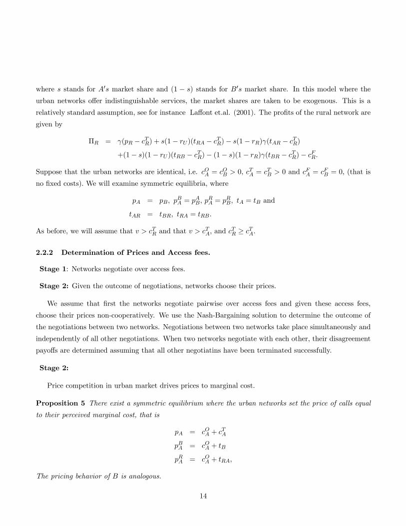
where s stands for A0s market share and (1 − s) stands for B0s market share. In this model where the

urban networks offer indistinguishable services, the market shares are taken to be exogenous. This is a

relatively standard assumption, see for instance Laffont et.al. (2001). The profits of the rural network are

given by

ΠR = γ(pR − cTR) + s(1− rU )(tRA − cTR)− s(1− rR)γ(tAR − cTR)

+(1− s)(1− rU )(tRB − cTR)− (1− s)(1− rR)γ(tBR − cTR)− cFR.

Suppose that the urban networks are identical, i.e. cOA = cOB > 0, cTA = cTB > 0 and cFA = cFB = 0, (that is

no fixed costs). We will examine symmetric equilibria, where

pA = pB, pBA = pAB, p

RA = pRB, tA = tB and

tAR = tBR, tRA = tRB.

As before, we will assume that v > cTR and that v > cTA, and cTR ≥ cTA.

2.2.2 Determination of Prices and Access fees.

Stage 1: Networks negotiate over access fees.

Stage 2: Given the outcome of negotiations, networks choose their prices.

We assume that first the networks negotiate pairwise over access fees and given these access fees,

choose their prices non-cooperatively. We use the Nash-Bargaining solution to determine the outcome of

the negotiations between two networks. Negotiations between two networks take place simultaneously and

independently of all other negotiations. When two networks negotiate with each other, their disagreement

payoffs are determined assuming that all other negotiatins have been terminated successfully.

Stage 2:

Price competition in urban market drives prices to marginal cost.

Proposition 5 There exist a symmetric equilibrium where the urban networks set the price of calls equal

to their perceived marginal cost, that is

pA = cOA + cTA

pBA = cOA + tB

pRA = cOA + tRA,

The pricing behavior of B is analogous.

14

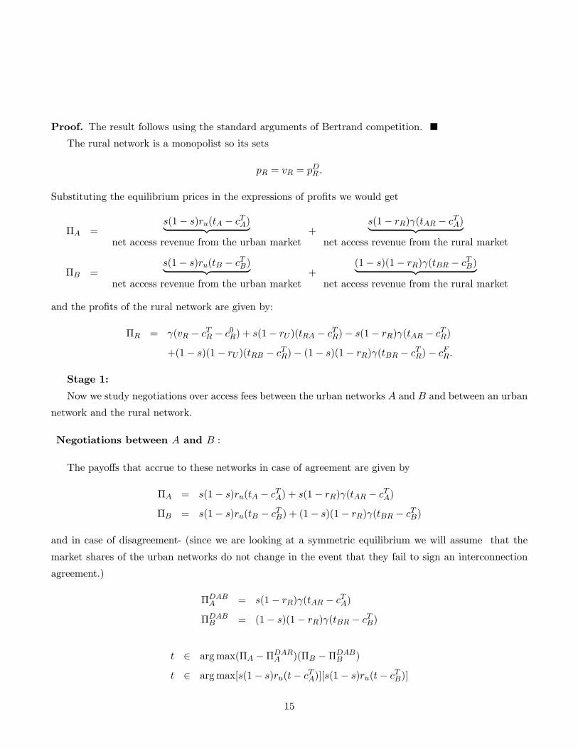
Proof. The result follows using the standard arguments of Bertrand competition.

The rural network is a monopolist so its sets

pR = vR = pDR .

Substituting the equilibrium prices in the expressions of profits we would get

ΠA =s(1− s)ru(tA − cTA)| {z }

net access revenue from the urban market+

s(1− rR)γ(tAR − cTA)| {z }net access revenue from the rural market

ΠB =s(1− s)ru(tB − cTB)| {z }

net access revenue from the urban market+

(1− s)(1− rR)γ(tBR − cTB)| {z }net access revenue from the rural market

and the profits of the rural network are given by:

ΠR = γ(vR − cTR − c0R) + s(1− rU )(tRA − cTR)− s(1− rR)γ(tAR − cTR)

+(1− s)(1− rU )(tRB − cTR)− (1− s)(1− rR)γ(tBR − cTR)− cFR.

Stage 1:

Now we study negotiations over access fees between the urban networks A and B and between an urban

network and the rural network.

Negotiations between A and B :

The payoffs that accrue to these networks in case of agreement are given by

ΠA = s(1− s)ru(tA − cTA) + s(1− rR)γ(tAR − cTA)

ΠB = s(1− s)ru(tB − cTB) + (1− s)(1− rR)γ(tBR − cTB)

and in case of disagreement- (since we are looking at a symmetric equilibrium we will assume that the

market shares of the urban networks do not change in the event that they fail to sign an interconnection

agreement.)

ΠDABA = s(1− rR)γ(tAR − cTA)

ΠDABB = (1− s)(1− rR)γ(tBR − cTB)

t ∈ argmax(ΠA −ΠDARA )(ΠB −ΠDAB

B )

t ∈ argmax[s(1− s)ru(t− cTA)][s(1− s)ru(t− cTB)]

15

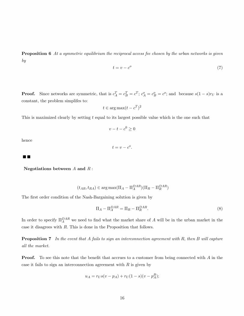
Proposition 6 At a symmetric equilibrium the reciprocal access fee chosen by the urban networks is given

by

t = v − co (7)

Proof. Since networks are symmetric, that is cTA = cTB = cT ; coA = coB = co; and because s(1− s)rU is a

constant, the problem simplifes to:

t ∈ argmax(t− cT )2

This is maximized clearly by setting t equal to its largest possible value which is the one such that

v − t− c0 ≥ 0

hence

t = v − co.

Negotiations between A and R :

(tAR, tRA) ∈ argmax(ΠA −ΠDARA )(ΠR −ΠDAR

R )

The first order condition of the Nash-Bargaining solution is given by

ΠA −ΠDARA = ΠR −ΠDAR

R . (8)

In order to specify ΠDARA we need to find what the market share of A will be in the urban market in the

case it disagrees with R. This is done in the Proposition that follows.

Proposition 7 In the event that A fails to sign an interconnection agreement with R, then B will capture

all the market.

Proof. To see this note that the benefit that accrues to a customer from being connected with A in the

case it fails to sign an interconnection agreement with R is given by

uA = rUs(v − pA) + rU (1− s)(v − pBA);

16

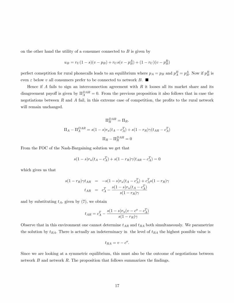
on the other hand the utility of a consumer connected to B is given by

uB = rU (1− s)(v − pB) + rUs(v − pAB) + (1− rU )(v − pRB)

perfect comeptition for rural phonecalls leads to an equilibrium where pA = pB and pBA = pAB. Now if pRB is

even ε below v all consumers prefer to be connected to network B.

Hence if A fails to sign an interconnection agreement with R it looses all its market share and its

disagreement payoff is given by ΠDARA = 0. From the previous proposition it also follows that in case the

negotiations between R and A fail, in this extreme case of competition, the profits to the rural network

will remain unchanged.

ΠDARR = ΠR.

ΠA −ΠDARA = s(1− s)ru(tA − cTA) + s(1− rR)γ(tAR − cTA)

ΠR −ΠDARR = 0

From the FOC of the Nash-Bargaining solution we get that

s(1− s)ru(tA − cTA) + s(1− rR)γ(tAR − cTA) = 0

which gives us that

s(1− rR)γtAR = −s(1− s)ru(tA − cTA) + cTAs(1− rR)γ

tAR = cTA −s(1− s)ru(tA − cTA)

s(1− rR)γ

and by substituting tA, given by (7), we obtain

tAR = cTA −s(1− s)ru(v − co − cTA)

s(1− rR)γ

Observe that in this environment one cannot determine tAR and tRA both simultaneously. We parametrize

the solution by tRA. There is actually an indeterminacy in the level of tRA the highest possible value is

tRA = v − co.

Since we are looking at a symmetric equilibrium, this must also be the outcome of negotiations between

network B and network R. The proposition that follows summarizes the findings.

17

Proposition 8 At a symmetric equilibrium, the access fee that the rural network pays to an urban network

is given by

tAR = tBR = cT − s(1− s)rU (v − co − cTA)

s(1− rR)γ

and the access fee that the urban network pays to an rural network is given by

tRA = tRB = v − co.

It is worth observing that the access fee that the rural network pays to an urban network in below the

cost of terminating the call. On the other hand the access fee that an urban network pays to the rural

network is equal to the value of the phone call minus the cost of originating the call. That is, via the

access fee the rural network can extract all the surplus - net of originating cost - that is generated from

interconnection. The reason for this is the extremely strong bargaining power that it has. This power

comes from the fact that R is the monopolist in selling access to rural customers. This together with the

fierce competition that the urban networks face, allows R to achieve extremely favorable interconnection

agreements.

Proposition 9 At a symmetric equilibrium, the profits of the networks are give by

ΠR = γ(vR − cTR − c0R) + (1− rU )(v − co − cTR) + s(1− s)ru(v − co − cT ) + (1− rR)γ¡cTR − cT

¢− cFR

ΠB = ΠA = 0.

Moreover the rural network’s profits are greater compared to the ones without interconnection.

Proof. Hence the rural network’s equilibrium profits are given by

ΠR = γ(vR − cTR − c0R) + (1− rU )(v − co − cTR)− (1− rR)γ

µcT − s(1− s)ru(v − co − cTA)

s(1− rR)γ− cTR

¶− cFR

= γ(vR − cTR − c0R) + (1− rU )(v − co − cTR) + (1− rR)γ

µs(1− s)ru(v − co − cTA)

s(1− rR)γ+ cTR − cT

¶− cFR

= γ(vR − cTR − c0R) + (1− rU )(v − co − cTR) + s(1− s)ru(v − co − cT ) + (1− rR)γ¡cTR − cT

¢− cFR

It is easy to see that the rural network’s profits without interconnection are

ΠNIR = γ(vR − cTR − c0R)− cFR.

Hence

ΠR −ΠNIR = (1− rU )(v − co − cTR) + (1− rR)γ

µs(1− s)ru(v − co − cTA)

s(1− rR)γ+ cTR − cT

¶> 0

since v > co + cTR and cTR > cT .

18

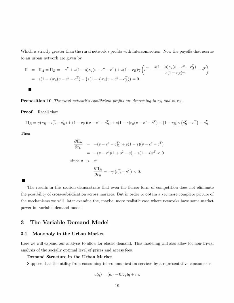
Which is strictly greater than the rural network’s profits with interconnection. Now the payoffs that accrue

to an urban network are given by

Π = ΠA = ΠB = −cF + s(1− s)ru(v − co − cT ) + s(1− rR)γ

µcT − s(1− s)ru(v − co − cTA)

s(1− rR)γ− cT

¶= s(1− s)ru(v − co − cT )− ¡s(1− s)ru(v − co − cTA)

¢= 0

Proposition 10 The rural network’s equilibrium profits are decreasing in rR and in rU .

Proof. Recall that

ΠR = γ(vR − cTR − c0R) + (1− rU )(v − co − cTR) + s(1− s)ru(v − co − cT ) + (1− rR)γ¡cTR − cT

¢− cFR

Then

∂ΠR∂rU

= −(v − co − cTR) + s(1− s)(v − co − cT )

= −(v − co)(1 + s2 − s)− s(1− s)cT < 0

since v > co

∂ΠR∂rR

= −γ ¡cTR − cT¢< 0.

The results in this section demonstrate that even the fiercer form of competition does not eliminate

the possibility of cross-subsidization across markets. But in order to obtain a yet more complete picture of

the mechanisms we will later examine the, maybe, more realistic case where networks have some market

power in variable demand model.

3 The Variable Demand Model

3.1 Monopoly in the Urban Market

Here we will expand our analysis to allow for elastic demand. This modeling will also allow for non-trivial

analysis of the socially optimal level of prices and access fees.

Demand Structure in the Urban Market

Suppose that the utility from consuming telecommunication services by a representative consumer is

u(q) = (aU − 0.5q)q +m.

19

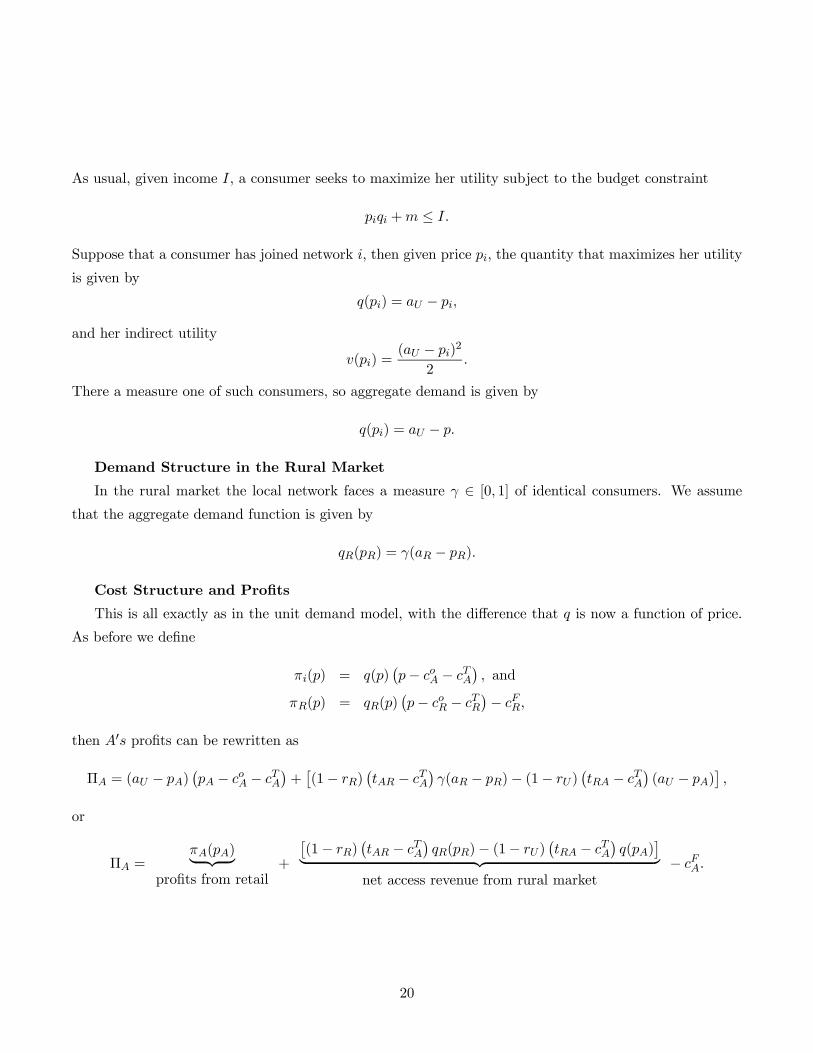
As usual, given income I, a consumer seeks to maximize her utility subject to the budget constraint

piqi +m ≤ I.

Suppose that a consumer has joined network i, then given price pi, the quantity that maximizes her utility

is given by

q(pi) = aU − pi,

and her indirect utility

v(pi) =(aU − pi)

2

2.

There a measure one of such consumers, so aggregate demand is given by

q(pi) = aU − p.

Demand Structure in the Rural Market

In the rural market the local network faces a measure γ ∈ [0, 1] of identical consumers. We assumethat the aggregate demand function is given by

qR(pR) = γ(aR − pR).

Cost Structure and Profits

This is all exactly as in the unit demand model, with the difference that q is now a function of price.

As before we define

πi(p) = q(p)¡p− coA − cTA

¢, and

πR(p) = qR(p)¡p− coR − cTR

¢− cFR,

then A0s profits can be rewritten as

ΠA = (aU − pA)¡pA − coA − cTA

¢+£(1− rR)

¡tAR − cTA

¢γ(aR − pR)− (1− rU )

¡tRA − cTA

¢(aU − pA)

¤,

or

ΠA =πA(pA)| {z }

profits from retail+

£(1− rR)

¡tAR − cTA

¢qR(pR)− (1− rU )

¡tRA − cTA

¢q(pA)

¤| {z }net access revenue from rural market

− cFA.

20

3.1.1 Ramsey Pricing

We would like to investigate what prices and access fees maximize welfare subject to the constraint that

none of the networks, that is the urban and the rural network, is running a loss. Let λ1 and λ2 denote the

Lagrangian multipliers associated with these constraints. Welfare is given by

W =

(aU − pA)2

2| {z }consumer surplus in urban market

+

γ(aR − pR)2

2| {z }consumer surplus in rural market

+(1 + λU )

¡πA(pA) +

£(1− rR)

¡tAR − cTA

¢γ(aR − pR)− (1− rU )

¡tRA − cTA

¢(aU − pA)

¤¢| {z }producer surplus in urban market

+(1 + λR)

¡πR(pR)− cFR +

£(1− rU )

¡tRA − cTR

¢(aU − pA)− (1− rR)

¡tAR − cTR

¢γ(aR − pR)

¤¢| {z }producer surplus in rural market

∂W

∂pU= −(aU − pA) + (1 + λU )

¡(aU − pA)−

¡pA − coA − cTA

¢+ (1− rU )

¡tRA − cTA

¢¢−(1 + λR)(1− rU )

¡tRA − cTR

¢= λU (aU − pA) + (1 + λU )

¡(1− rU )

¡tRA − cTA

¢− ¡pA − coA − cTA¢¢− (1 + λR)(1− rU )

¡tRA − cTR

¢= λUaU + (1 + λU)

¡(1− rU )

¡tRA − cTA

¢+ coA + cTA

¢− (1 + λR)(1− rU )¡tRA − cTR

¢− (1 + 2λU )pA = 0which gives

pA =λUaU + (1 + λU )

¡(1− rU )

¡tRA − cTA

¢+ coA + cTA

¢− (1 + λR)(1− rU )¡tRA − cTR

¢(1 + 2λU )

∂W

∂pR= −γ(aR − pR)− (1 + λU )(1− rR)

¡tAR − cTA

¢γ

+(1 + λR)¡γ(aR − pR)− γpR + γcoR + γcTR − cFR + (1− rR)

¡tAR − cTR

¢γ¢

= λRγ(aR − pR)− (1 + λU )(1− rR)¡tAR − cTA

¢γ + (1 + λR)

¡−γpR + γcoR + γcTR − cFR + (1− rR)¡tAR − cTR

¢γ

= λRγaR − (1 + λU )(1− rR)¡tAR − cTA

¢γ + (1 + λR)

¡γcoR + γcTR − cFR + (1− rR)

¡tAR − cTR

¢γ¢− (1 + 2λR)pR

pR =λRγaR − (1 + λU )(1− rR)

¡tAR − cTA

¢γ + (1 + λR)

¡γcoR + γcTR − cFR + (1− rR)

¡tAR − cTR

¢γ¢

(1 + 2λR)

Now let us look for the welfare maximizing access fees.

∂W

∂tAR= (1 + λU ) ((1− rR)γ(aR − pR))− (1 + λR) ((1− rR)γ(aR − pR))

∂W

∂tRA= −(1 + λU )(1− rU ) (aU − pA) + (1 + λR)(1− rU ) (aU − pA)

21

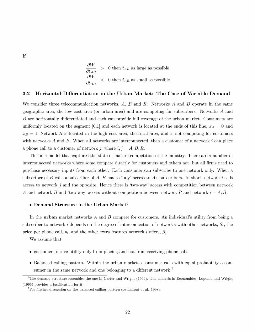
If

∂W

∂tAR> 0 then tAR as large as possible

∂W

∂tAR< 0 then tAR as small as possible

3.2 Horizontal Differentiation in the Urban Market: The Case of Variable Demand

We consider three telecommunication networks, A, B and R. Networks A and B operate in the same

geographic area, the low cost area (or urban area) and are competing for subscribers. Networks A and

B are horizontally differentiated and each can provide full coverage of the urban market. Consumers are

uniformly located on the segment [0,1] and each network is located at the ends of this line, xA = 0 and

xB = 1. Network R is located in the high cost area, the rural area, and is not competing for customers

with networks A and B. When all networks are interconnected, then a customer of a network i can place

a phone call to a customer of network j, where i, j = A,B,R.

This is a model that captures the state of mature competition of the industry. There are a number of

interconnected networks where some compete directly for customers and others not, but all firms need to

purchase necessary inputs from each other. Each consumer can subscribe to one network only. When a

subscriber of B calls a subscriber of A, B has to ‘buy’ access to A’s subscribers. In short, network i sells

access to network j and the opposite. Hence there is ‘two-way’ access with competition between network

A and network B and ‘two-way’ access without competition between network R and network i = A,B.

• Demand Structure in the Urban Market6

In the urban market networks A and B compete for customers. An individual’s utility from being a

subscriber to network i depends on the degree of interconnection of network i with other networks, Si, the

price per phone call, pi, and the other extra features network i offers, βi.

We assume that

• consumers derive utility only from placing and not from receiving phone calls

• Balanced calling pattern. Within the urban market a consumer calls with equal probability a con-sumer in the same network and one belonging to a different network.7

6The demand structure resembles the one in Carter and Wright (1999). The analysis in Economides, Lopomo and Wright

(1996) provides a justification for it.7For further discussion on the balanced calling pattern see Laffont et al. 1998a.

22

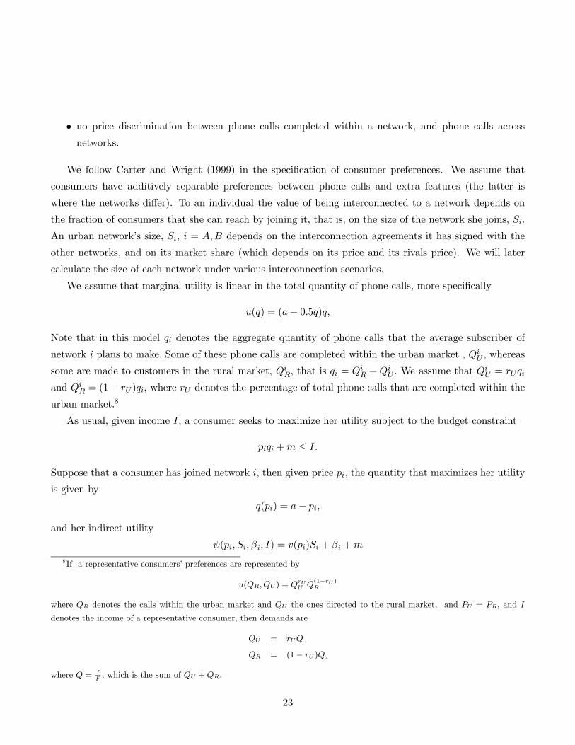
• no price discrimination between phone calls completed within a network, and phone calls acrossnetworks.

We follow Carter and Wright (1999) in the specification of consumer preferences. We assume that

consumers have additively separable preferences between phone calls and extra features (the latter is

where the networks differ). To an individual the value of being interconnected to a network depends on

the fraction of consumers that she can reach by joining it, that is, on the size of the network she joins, Si.

An urban network’s size, Si, i = A,B depends on the interconnection agreements it has signed with the

other networks, and on its market share (which depends on its price and its rivals price). We will later

calculate the size of each network under various interconnection scenarios.

We assume that marginal utility is linear in the total quantity of phone calls, more specifically

u(q) = (a− 0.5q)q,

Note that in this model qi denotes the aggregate quantity of phone calls that the average subscriber of

network i plans to make. Some of these phone calls are completed within the urban market , QiU , whereas

some are made to customers in the rural market, QiR, that is qi = Qi

R +QiU . We assume that Q

iU = rUqi

and QiR = (1− rU )qi, where rU denotes the percentage of total phone calls that are completed within the

urban market.8

As usual, given income I, a consumer seeks to maximize her utility subject to the budget constraint

piqi +m ≤ I.

Suppose that a consumer has joined network i, then given price pi, the quantity that maximizes her utility

is given by

q(pi) = a− pi,

and her indirect utility

ψ(pi, Si, βi, I) = v(pi)Si + βi +m

8 If a representative consumers’ preferences are represented by

u(QR, QU ) = QrUU Q

(1−rU )R

where QR denotes the calls within the urban market and QU the ones directed to the rural market, and PU = PR, and I

denotes the income of a representative consumer, then demands are

QU = rUQ

QR = (1− rU )Q,

where Q = IP, which is the sum of QU +QR.

23

where

v(pi) =(a− pi)

2

2;

m represents the consumption of other goods, βi stands for the extras associated with being connected to

network i, and Si is the degree of interconnection of network i, i = A,B.

• Demand Structure in the Rural Market

In the rural market the local network faces a unit measure of identical consumers.9 Since there is only

one network in the rural market, we will not model explicitly the utility that an individual enjoys by being

connected to the network. We will focus on the aggregate demand function, which we will assume for

simplicity that it is given by

qR(pR) = γ(a− pR),

where γ ∈ [0, 1] and qR(pR) denotes the aggregate quantity of phone calls that the average subscriber of

the rural network plans to make at price pR. The total quantity of phone calls equals the sum of calls

directed to urban customers, QRU , and calls directed to rural consumers, Q

RR, that is qR = QR

R +QRU . We

assume that QRU = (1− rR)qR and QR

R = rRqR, where rR is the fraction of total calls made by the average

rural customer that are completed within the rural market.

We now determine the size of network i, Si under different degrees of interconnection.

• Size of the networks

Table (1) contains the size of a network for different cases of interconnection agreements taking the

market shares of A and B as given. We use s to denote A0s market share in case all networks have signed

interconnection agreements, s1 is A0s share when negotiations between A and B fail, s2 is A0s market share

when negotiations between A and R fail, and finally s3 is A0s share when negotiations between B and R

fail. If A has signed interconnection agreements with B and R, then SA = 1, and a subscriber of network

A can reach a subscriber j irrespective of the network that j belongs. If it has signed an interconnection

agreement only with B then SA = rU , (the rural customers cannot be reached by a subscriber of A), and

finally if it has signed an interconnection agreement with R only, SA = rUs + (1 − rU ), where s denotes

A0s market share.

• Market shares when the urban networks are interconnected to each other: SA = SB = 1.

9Or alternatively, one representative consumer.

24

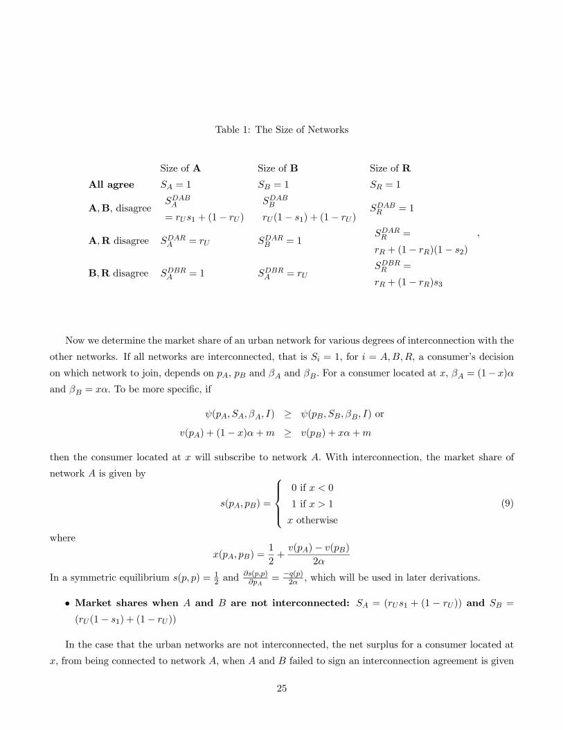
Table 1: The Size of Networks

Size of A Size of B Size of R

All agree SA = 1 SB = 1 SR = 1

A,B, disagreeSDABA

= rUs1 + (1− rU )

SDABB

rU(1− s1) + (1− rU )SDABR = 1

A,R disagree SDARA = rU SDAR

B = 1SDARR =

rR + (1− rR)(1− s2)

B,R disagree SDBRA = 1 SDBR

A = rUSDBRR =

rR + (1− rR)s3

,

Now we determine the market share of an urban network for various degrees of interconnection with the

other networks. If all networks are interconnected, that is Si = 1, for i = A,B,R, a consumer’s decision

on which network to join, depends on pA, pB and βA and βB. For a consumer located at x, βA = (1− x)α

and βB = xα. To be more specific, if

ψ(pA, SA, βA, I) ≥ ψ(pB, SB, βB, I) or

v(pA) + (1− x)α+m ≥ v(pB) + xα+m

then the consumer located at x will subscribe to network A. With interconnection, the market share of

network A is given by

s(pA, pB) =

0 if x < 0

1 if x > 1

x otherwise

(9)

where

x(pA, pB) =1

2+

v(pA)− v(pB)

2α

In a symmetric equilibrium s(p, p) = 12 and

∂s(p,p)∂pA

= −q(p)2α , which will be used in later derivations.

• Market shares when A and B are not interconnected: SA = (rUs1 + (1 − rU )) and SB =

(rU (1− s1) + (1− rU ))

In the case that the urban networks are not interconnected, the net surplus for a consumer located at

x, from being connected to network A, when A and B failed to sign an interconnection agreement is given

25

by

v(pA)(rUs1 + (1− rU )) + (1− x)α,

and the net surplus from being connected to network B is given by

v(pB)(rU (1− s1) + (1− rU )) + αx,

where s1 stands for network A0s market share, for the case that urban firms fail to reach an agreement,

and pi denotes the price of network i, i = A,B. With no interconnection between A and B, network A0s

market share is given by

s1 =

0 if x1 < 0

1 if x1 > 1

x1 otherwise

(10)

where

x1(pA, pB) =α− v(pB) + v(pA)(1− rU )

2α− (v(pA) + v(pB))rU. (11)

Network B0s market share is given by 1 − s1. In a symmetric equilibrium, pA = pB and s1 =12 and

∂s1(p,p)∂pA

= (a−p)(2−rU )4(α−v(p)) .

• Market shares when A and R are not interconnected: SA = rU and SB = 1

When A and R fail to sign an interconnection agreement, the net surplus for a consumer located at x,

is given by

v(pA)rU + (1− x)α+m,

and the net surplus from being connected to network B is given by

v(pB) + αx+m.

With no interconnection between A and R, network A0s market share is given by

s2 =

0 if x2 < 0

1 if x2 > 1

x2 otherwise

(12)

where

x2(pA, pB) =1

2+

v(pA)rU − v(pB)

2α. (13)

Network B0s market share is given by 1− s2.

26

• Market shares when B and R are not interconnected: SA = 1 and SB = rU

Using the, by now familiar, procedure, we get that with no interconnection between B and R, network

A0s market share is given by

s3 =

0 if x3 < 0

1 if x3 > 1

x3 otherwise

where

x3(pA, pB) =1

2+

v(pA)− v(pB)rU2α

. (14)

Network B0s market share is given by 1− s3.

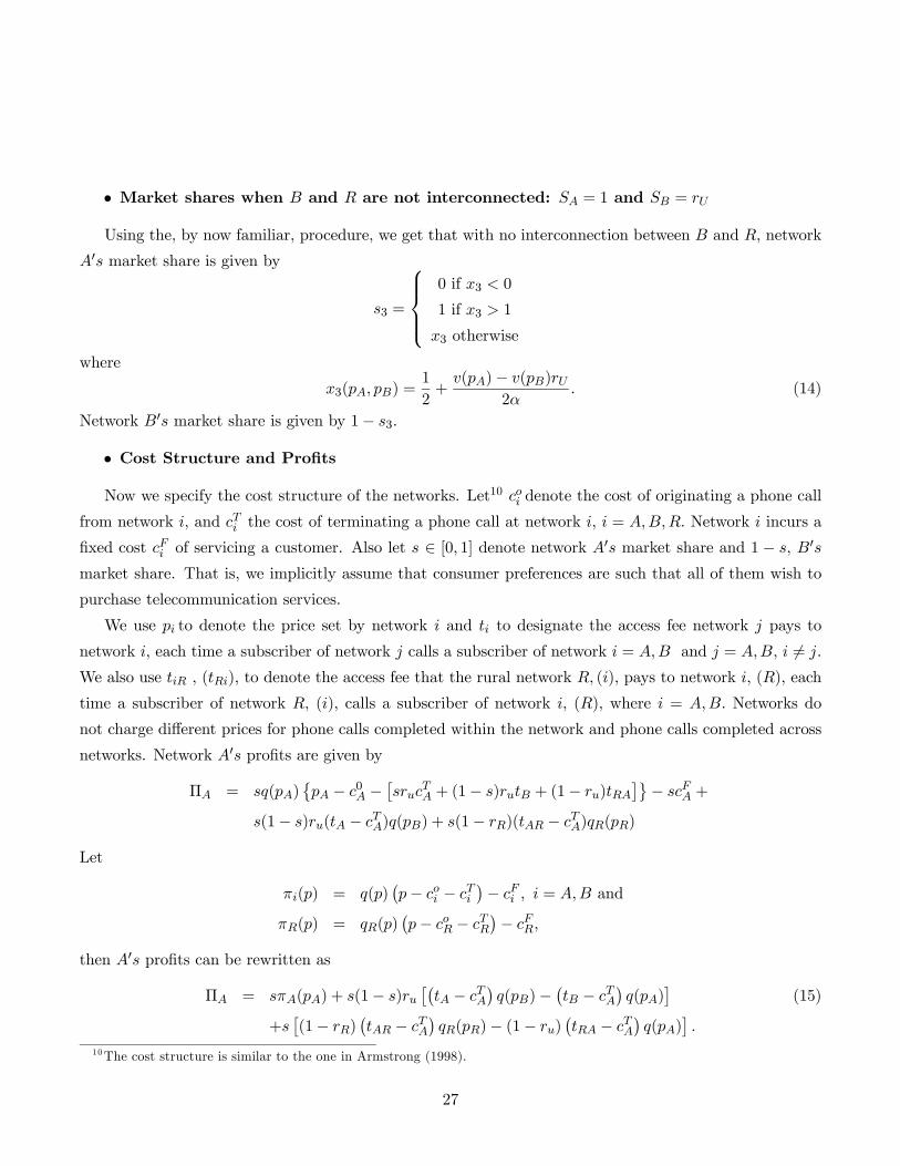
• Cost Structure and Profits

Now we specify the cost structure of the networks. Let10 coi denote the cost of originating a phone call

from network i, and cTi the cost of terminating a phone call at network i, i = A,B,R. Network i incurs a

fixed cost cFi of servicing a customer. Also let s ∈ [0, 1] denote network A0s market share and 1 − s, B0s

market share. That is, we implicitly assume that consumer preferences are such that all of them wish to

purchase telecommunication services.

We use pi to denote the price set by network i and ti to designate the access fee network j pays to

network i, each time a subscriber of network j calls a subscriber of network i = A,B and j = A,B, i 6= j.

We also use tiR , (tRi), to denote the access fee that the rural network R, (i), pays to network i, (R), each

time a subscriber of network R, (i), calls a subscriber of network i, (R), where i = A,B. Networks do

not charge different prices for phone calls completed within the network and phone calls completed across

networks. Network A0s profits are given by

ΠA = sq(pA)©pA − c0A −

£sruc

TA + (1− s)rutB + (1− ru)tRA

¤ª− scFA +

s(1− s)ru(tA − cTA)q(pB) + s(1− rR)(tAR − cTA)qR(pR)

Let

πi(p) = q(p)¡p− coi − cTi

¢− cFi , i = A,B and

πR(p) = qR(p)¡p− coR − cTR

¢− cFR,

then A0s profits can be rewritten as

ΠA = sπA(pA) + s(1− s)ru£¡tA − cTA

¢q(pB)−

¡tB − cTA

¢q(pA)

¤(15)

+s£(1− rR)

¡tAR − cTA

¢qR(pR)− (1− ru)

¡tRA − cTA

¢q(pA)

¤.

10The cost structure is similar to the one in Armstrong (1998).

27

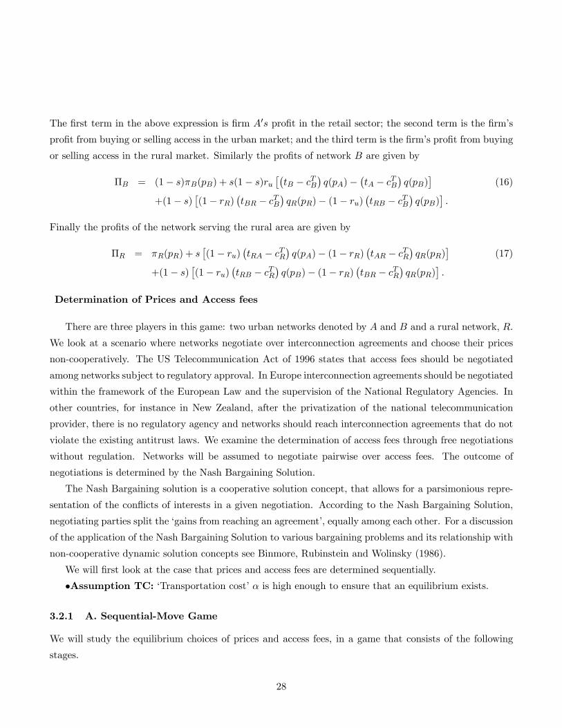
The first term in the above expression is firm A0s profit in the retail sector; the second term is the firm’s

profit from buying or selling access in the urban market; and the third term is the firm’s profit from buying

or selling access in the rural market. Similarly the profits of network B are given by

ΠB = (1− s)πB(pB) + s(1− s)ru£¡tB − cTB

¢q(pA)−

¡tA − cTB

¢q(pB)

¤(16)

+(1− s)£(1− rR)

¡tBR − cTB

¢qR(pR)− (1− ru)

¡tRB − cTB

¢q(pB)

¤.

Finally the profits of the network serving the rural area are given by

ΠR = πR(pR) + s£(1− ru)

¡tRA − cTR

¢q(pA)− (1− rR)

¡tAR − cTR

¢qR(pR)

¤(17)

+(1− s)£(1− ru)

¡tRB − cTR

¢q(pB)− (1− rR)

¡tBR − cTR

¢qR(pR)

¤.

Determination of Prices and Access fees

There are three players in this game: two urban networks denoted by A and B and a rural network, R.

We look at a scenario where networks negotiate over interconnection agreements and choose their prices

non-cooperatively. The US Telecommunication Act of 1996 states that access fees should be negotiated

among networks subject to regulatory approval. In Europe interconnection agreements should be negotiated

within the framework of the European Law and the supervision of the National Regulatory Agencies. In

other countries, for instance in New Zealand, after the privatization of the national telecommunication

provider, there is no regulatory agency and networks should reach interconnection agreements that do not

violate the existing antitrust laws. We examine the determination of access fees through free negotiations

without regulation. Networks will be assumed to negotiate pairwise over access fees. The outcome of

negotiations is determined by the Nash Bargaining Solution.

The Nash Bargaining solution is a cooperative solution concept, that allows for a parsimonious repre-

sentation of the conflicts of interests in a given negotiation. According to the Nash Bargaining Solution,

negotiating parties split the ‘gains from reaching an agreement’, equally among each other. For a discussion

of the application of the Nash Bargaining Solution to various bargaining problems and its relationship with

non-cooperative dynamic solution concepts see Binmore, Rubinstein and Wolinsky (1986).

We will first look at the case that prices and access fees are determined sequentially.

•Assumption TC: ‘Transportation cost’ α is high enough to ensure that an equilibrium exists.

3.2.1 A. Sequential-Move Game

We will study the equilibrium choices of prices and access fees, in a game that consists of the following

stages.

28

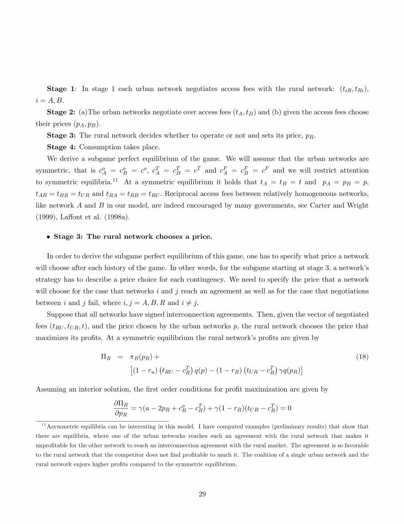
Stage 1: In stage 1 each urban network negotiates access fees with the rural network: (tiR, tRi),

i = A,B.

Stage 2: (a)The urban networks negotiate over access fees (tA, tB) and (b) given the access fees choose

their prices (pA, pB).

Stage 3: The rural network decides whether to operate or not and sets its price, pR.

Stage 4: Consumption takes place.

We derive a subgame perfect equilibrium of the game. We will assume that the urban networks are

symmetric, that is coA = coB = co, cTA = cTB = cT and cFA = cFB = cF and we will restrict attention

to symmetric equilibria.11 At a symmetric equilibrium it holds that tA = tB = t and pA = pB = p,

tAR = tBR = tUR and tRA = tRB = tRU . Reciprocal access fees between relatively homogeneous networks,

like network A and B in our model, are indeed encouraged by many governments, see Carter and Wright

(1999), Laffont et al. (1998a).

• Stage 3: The rural network chooses a price.

In order to derive the subgame perfect equilibrium of this game, one has to specify what price a network

will choose after each history of the game. In other words, for the subgame starting at stage 3, a network’s

strategy has to describe a price choice for each contingency. We need to specify the price that a network

will choose for the case that networks i and j reach an agreement as well as for the case that negotiations

between i and j fail, where i, j = A,B,R and i 6= j.

Suppose that all networks have signed interconnection agreements. Then, given the vector of negotiated

fees (tRU , tUR, t), and the price chosen by the urban networks p, the rural network chooses the price that

maximizes its profits. At a symmetric equilibrium the rural network’s profits are given by

ΠR = πR(pR) + (18)£(1− ru)

¡tRU − cTR

¢q(p)− (1− rR)

¡tUR − cTR

¢γq(pR)

¤Assuming an interior solution, the first order conditions for profit maximization are given by

∂ΠR∂pR

= γ(a− 2pR + coR − cTR) + γ(1− rR)(tUR − cTR) = 0

11Asymmetric equilibria can be interesting in this model. I have computed examples (preliminary results) that show that

there are equilibria, where one of the urban networks reaches such an agreement with the rural network that makes it

unprofitable for the other network to reach an interconnection agreement with the rural market. The agreement is so favorable

to the rural network that the competitor does not find profitable to much it. The coalition of a single urban network and the

rural network enjoys higher profits compared to the symmetric equilibrium.

29

which gives

pR =a+ coR + cTR + (tUR − cTR)(1− rR)

2.

Using this straightforward procedure one can determine the price that the urban network will charge in

different histories, when for instance negotiations between R and A fail.

• Stage 2: Urban Networks Choose Access Fees and Prices

Suppose that the urban networks have agreed on a reciprocal access fee t and the negotiations with the

rural network have already taken place. Given t and (tUR, tRU ), we derive a symmetric equilibrium of the

price game between network A and network B. Consider network A; its profits are given by (15). Let us

define RAR(pR, p) by

RAR(pR, p) = (1− rR)¡tUR − cT

¢qR(pR)− (1− ru)

¡tRU − cT

¢q(p).

This is A0s net revenue from selling access to R. Assume an interior solution. If pA is a profit maximizing

price then it satisfies

∂ΠA(p, p)

∂pA=

∂s(p, p)

∂pAπA(p) + s(p, p)

∂πA(p)

∂pA− s(1− s)ru(t− cT )

∂q(p)

∂pA

+∂s(p, p)

∂pARAR(pR, p) + s(p, p)

∂RAR(pR, p)

∂pA= 0.

Access Fees: From the analysis in Armstrong (1998), Carter and Wright (1999) and Laffont, Rey and

Tirole (1998a) we know that if an equilibrium exists, and access fees are required to be reciprocal, then

in a deregulated duopoly market, networks will choose access fees that support prices that maximize joint

profits. In our environment, where the urban networks are interconnected with the rural network, they

will choose access fees that support the price that maximizes joint profit.

Joint profit for networks A and B are given by

ΠA+B(p) = π(p) +RAR(pR, p)

and assuming an interior solution, the FOC for joint profit maximization is given by

∂π(p)

∂p+

∂RAR(pR, p)

∂p= 0. (19)

The price that maximizes joint profits is given by

p =a+ co + cT + (1− rU )(tRU − cT )

2. (20)

30

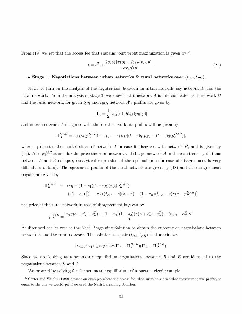
From (19) we get that the access fee that sustains joint profit maximization is given by12

t = cT +2q(p) [π(p) +RAR(pR, p)]

−αruq0(p) . (21)

• Stage 1: Negotiations between urban networks & rural networks over (tUR, tRU ).

Now, we turn on the analysis of the negotiations between an urban network, say network A, and the

rural network. From the analysis of stage 2, we know that if network A is interconnected with network B

and the rural network, for given tUR and tRU , network A0s profits are given by

ΠA =1

2[π(p) +RAR(pR, p)]

and in case network A disagrees with the rural network, its profits will be given by

ΠDARA = s1rUπ(p

DARA ) + s1(1− s1)rU [(t− c)q(pB)− (t− c)q(pDAR

A )],

where s1 denotes the market share of network A in case it disagrees with network R, and is given by

(11). Also pDARA stands for the price the rural network will charge network A in the case that negotiations

between A and R collapse, (analytical expression of the optimal price in case of disagreement is very

difficult to obtain). The agreement profits of the rural network are given by (18) and the disagreement

payoffs are given by

ΠDARR = (rR + (1− s1)(1− rR))πR(p

DARR )

+(1− s1)£(1− rU ) (tRU − c)(a− p)− (1− rR)(tUR − c)γ(a− pDAR

R )¤

the price of the rural network in case of disagreement is given by

pDARR =

rRγ(a+ coR + cTR) + (1− rR)(1− s2)(γ(a+ coR + cTR) + (tUR − cRT )γ)

2

As discussed earlier we use the Nash Bargaining Solution to obtain the outcome on negotiations between

network A and the rural network. The solution is a pair (tRA, tAR) that maximizes

(tAR, tRA) ∈ argmax(ΠA −ΠDARA )(ΠR −ΠDAR

R ).

Since we are looking at a symmetric equilibrium negotiations, between R and B are identical to the

negotiations between R and A.

We proceed by solving for the symmetric equilibrium of a parametrized example.12Carter and Wright (1999) present an example where the access fee that sustains a price that maximizes joins profits, is

equal to the one we would get if we used the Nash Bargaining Solution.

31

Table 2: Sequential-Moves: Symmetric Equilibrium: A

cFR = 9, rR = 0.5,

rU= 0.2

cFR = 9, rR = 0.5,

rU= 0.6

pA = pB 6.9058 6.4754

pR 6.1082 6.3392

pDARA = pDBR

B 6.5581 5.7383

pDARR = pDBR

R 6.3776 6.5550

tA = tB 5.3791 3.5657

ΠR 1.7032 −0.3580ΠDARR = ΠDBR

R −0.1954 −1.3257ΠA = ΠB 3.5381 5.4595

ΠDARA = ΠDBR

B 1.3801 4.4229

tRA = tRB 3.2645 3.3771

tAR = tBR −1.5672 −0.6431

cFR = 9, rR = 0.5,

rU= 0.9

6.1333

6.4870

5.4590

6.6663

3.4106

−2.1852−2.24097.0137

6.9580

3.6663

−0.0519

Suppose that

q(p) = 10− p

co = cT = 1, cF = 0, coR = cTR = 2

γ = 0.5, α = 50

As noted earlier we solve for a symmetric equilibrium, and we do not impose any cross market price

restrictions.

Discussion of the Results

Table 2 contains the equilibrium prices, access fees and profits that accrue to the three networks as we

increase rU . Recall that rU denotes the fraction of total calls made by urban customers that are completed

within the urban market. As rU increases, the less value the urban customers place in being interconnected

with the rural market. The equilibrium profits of the rural network decrease as rU increases. Later we will

verify analytically that this is also the case in alternative scenarios regarding the degree of competition

in the urban market. In the above example the profits that would accrue to the rural network if it were

not interconnected with the urban market, are given by πR = −4.5, when cFR = 9 and πR = −0.5, when

32

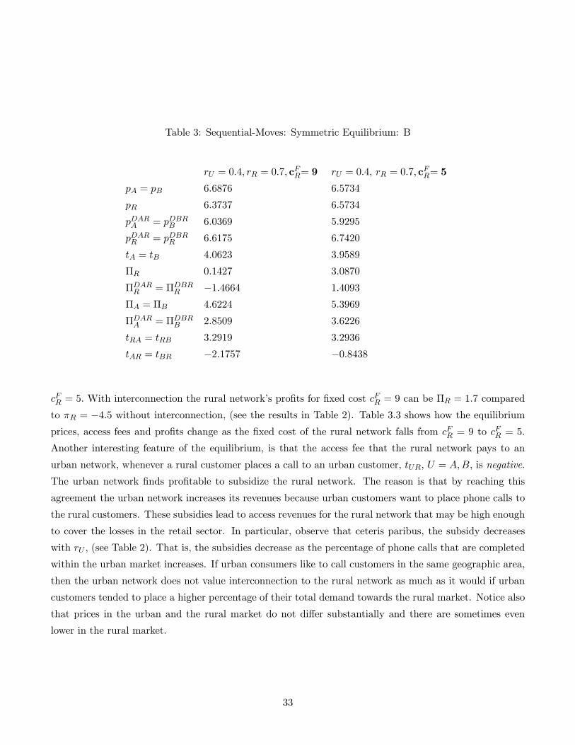
Table 3: Sequential-Moves: Symmetric Equilibrium: B

pA = pB

pR

pDARA = pDBR

B

pDARR = pDBR

R

tA = tB

ΠR

ΠDARR = ΠDBR

R

ΠA = ΠB

ΠDARA = ΠDBR

B

tRA = tRB

tAR = tBR

rU = 0.4, rR = 0.7, cFR= 9

6.6876

6.3737

6.0369

6.6175

4.0623

0.1427

−1.46644.6224

2.8509

3.2919

−2.1757

rU = 0.4, rR = 0.7, cFR= 5

6.5734

6.5734

5.9295

6.7420

3.9589

3.0870

1.4093

5.3969

3.6226

3.2936

−0.8438

cFR = 5. With interconnection the rural network’s profits for fixed cost cFR = 9 can be ΠR = 1.7 compared

to πR = −4.5 without interconnection, (see the results in Table 2). Table 3.3 shows how the equilibriumprices, access fees and profits change as the fixed cost of the rural network falls from cFR = 9 to cFR = 5.

Another interesting feature of the equilibrium, is that the access fee that the rural network pays to an

urban network, whenever a rural customer places a call to an urban customer, tUR, U = A,B, is negative.

The urban network finds profitable to subsidize the rural network. The reason is that by reaching this

agreement the urban network increases its revenues because urban customers want to place phone calls to

the rural customers. These subsidies lead to access revenues for the rural network that may be high enough

to cover the losses in the retail sector. In particular, observe that ceteris paribus, the subsidy decreases

with rU , (see Table 2). That is, the subsidies decrease as the percentage of phone calls that are completed

within the urban market increases. If urban consumers like to call customers in the same geographic area,

then the urban network does not value interconnection to the rural network as much as it would if urban

customers tended to place a higher percentage of their total demand towards the rural market. Notice also

that prices in the urban and the rural market do not differ substantially and there are sometimes even

lower in the rural market.

33

3.2.2 B. Simultaneous-Moves

We assume an interior solution and derive the first order conditions that optimal prices must satisfy. Taking

(pk, tA, tB, tAR, tRA, tBR, tRB) as given, k = A,B,R and k 6= i, network i chooses pi that solves

∂Πi∂pi

= 0 . (pi)

Simultaneously with choosing prices, networks negotiate pairwise in order to determine interconnection

access fees. In particular, network A negotiates with network B over tA and tB, and network R negotiates

with A and B over the determination of tAR, tRA and tBR and tRB. All negotiations take place simultane-

ously and independently from one another, in other words, we assume that the outcome of the negotiations

between R and A is not known to R and B when they bargain over (tBR, tRB).

• Negotiations between A and B over (tA, tB)

As noted earlier we will use the Nash Bargaining solution in order to determine the outcome of nego-

tiations between A and B. The Nash Solution to this bargaining situation is a pair (tA, tB) such that

(tA, tB) ∈ argmax(ΠA −ΠDABA )(ΠB −ΠDAB

B ), (22)

where ΠA and ΠB are given by (15) and (16) respectively. The disagreement payoffs of network A are

given by

ΠDABA = s1(rUs1 + (1− rU ))πA(pA) +

s1£(1− rR)

¡tAR − cTA

¢γq(pR)− (1− ru)

¡tRA − cTA

¢q(pA)

¤where s1 is given by (11). Similarly the disagreement payoffs of network B are given by

ΠDABB = (1− s1)(rU (1− s1) + (1− rU ))πB(pB) +

(1− s1)£(1− rR)

¡tBR − cTB

¢γq(pR)− (1− ru)

¡tRB − cTB

¢q(pB)

¤.

The first order conditions of the problem described in (22) reduce to

ΠA −ΠDABA −ΠB +ΠDAB

B = 0. (23)

• Negotiations between U and R over (tUR, tRU ), U = A,B

Networks A and R bargain over the determination of (tAR, tRA). Again, we use the Nash Solution to

determine the outcome of these negotiations. Hence

(tAR, tRA) ∈ argmax(ΠA −ΠDARA )(ΠR −ΠDAR

R ), (NAB)

34

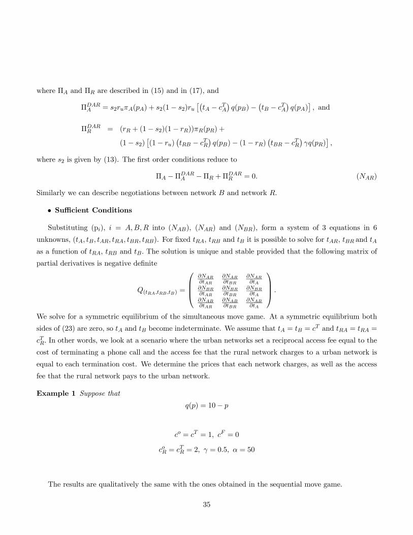
where ΠA and ΠR are described in (15) and in (17), and

ΠDARA = s2ruπA(pA) + s2(1− s2)ru

£¡tA − cTA

¢q(pB)−

¡tB − cTA

¢q(pA)

¤, and

ΠDARR = (rR + (1− s2)(1− rR))πR(pR) +

(1− s2)£(1− ru)

¡tRB − cTR

¢q(pB)− (1− rR)

¡tBR − cTR

¢γq(pR)

¤,

where s2 is given by (13). The first order conditions reduce to

ΠA −ΠDARA −ΠR +ΠDAR

R = 0. (NAR)

Similarly we can describe negotiations between network B and network R.

• Sufficient Conditions

Substituting (pi), i = A,B,R into (NAB), (NAR) and (NBR), form a system of 3 equations in 6

unknowns, (tA, tB, tAR, tRA, tBR, tRB). For fixed tRA, tRB and tB it is possible to solve for tAR, tBR and tA

as a function of tRA, tRB and tB. The solution is unique and stable provided that the following matrix of

partial derivatives is negative definite

Q(tRA,tRB ,tB) =

∂NAR∂tAR

∂NAR∂tBR

∂NAR∂tA

∂NBR∂tAR

∂NBR∂tBR

∂NBR∂tA

∂NAB∂tAR

∂NAB∂tBR

∂NAB∂tA

.

We solve for a symmetric equilibrium of the simultaneous move game. At a symmetric equilibrium both

sides of (23) are zero, so tA and tB become indeterminate. We assume that tA = tB = cT and tRA = tRA =

cTR. In other words, we look at a scenario where the urban networks set a reciprocal access fee equal to the

cost of terminating a phone call and the access fee that the rural network charges to a urban network is

equal to each termination cost. We determine the prices that each network charges, as well as the access

fee that the rural network pays to the urban network.

Example 1 Suppose that

q(p) = 10− p

co = cT = 1, cF = 0

coR = cTR = 2, γ = 0.5, α = 50

The results are qualitatively the same with the ones obtained in the sequential move game.

35

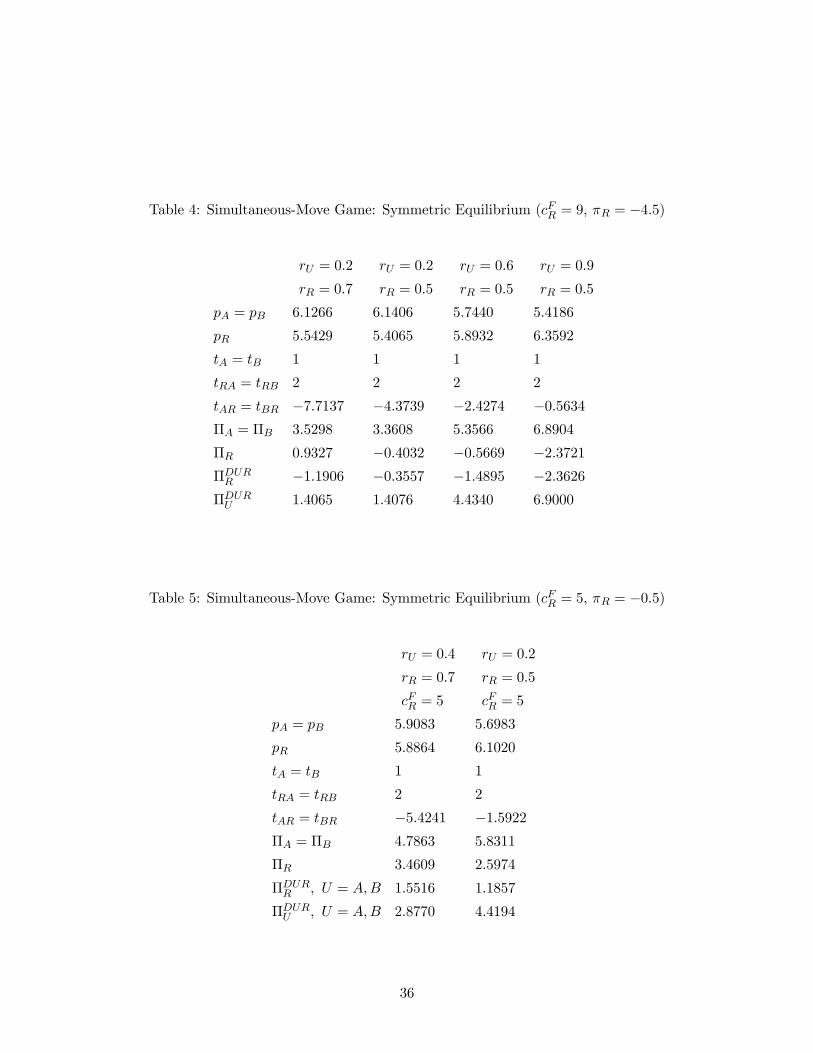
Table 4: Simultaneous-Move Game: Symmetric Equilibrium (cFR = 9, πR = −4.5)

rU = 0.2

rR = 0.7

rU = 0.2

rR = 0.5

rU = 0.6

rR = 0.5

rU = 0.9

rR = 0.5

pA = pB 6.1266 6.1406 5.7440 5.4186

pR 5.5429 5.4065 5.8932 6.3592

tA = tB 1 1 1 1

tRA = tRB 2 2 2 2

tAR = tBR −7.7137 −4.3739 −2.4274 −0.5634ΠA = ΠB 3.5298 3.3608 5.3566 6.8904

ΠR 0.9327 −0.4032 −0.5669 −2.3721ΠDURR −1.1906 −0.3557 −1.4895 −2.3626ΠDURU 1.4065 1.4076 4.4340 6.9000

Table 5: Simultaneous-Move Game: Symmetric Equilibrium (cFR = 5, πR = −0.5)

rU = 0.4

rR = 0.7

cFR = 5

rU = 0.2

rR = 0.5

cFR = 5

pA = pB 5.9083 5.6983

pR 5.8864 6.1020

tA = tB 1 1

tRA = tRB 2 2

tAR = tBR −5.4241 −1.5922ΠA = ΠB 4.7863 5.8311

ΠR 3.4609 2.5974

ΠDURR , U = A,B 1.5516 1.1857

ΠDURU , U = A,B 2.8770 4.4194

36

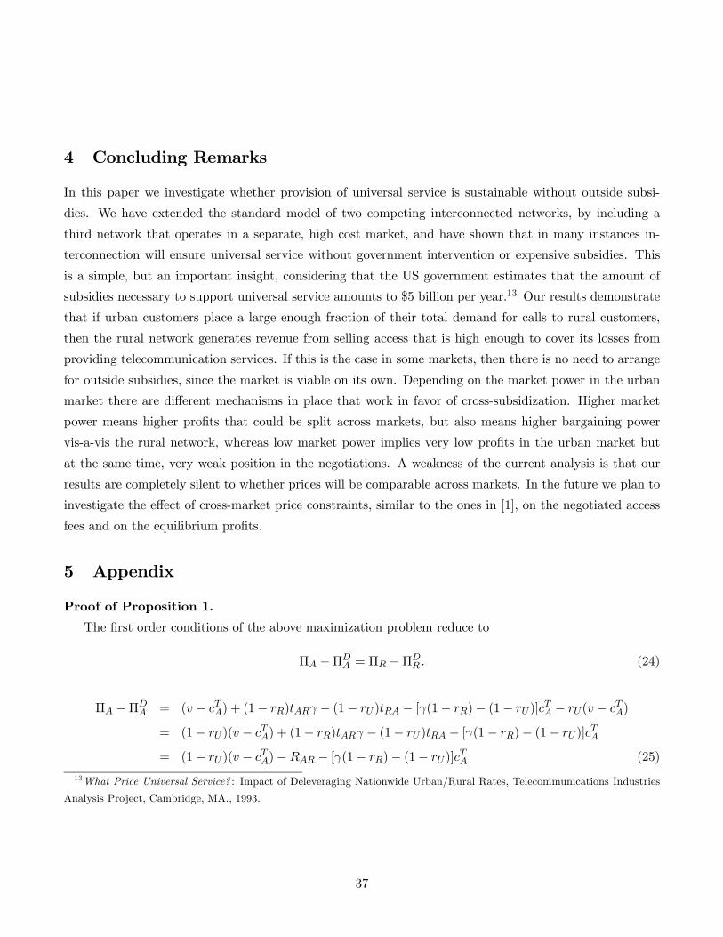
4 Concluding Remarks

In this paper we investigate whether provision of universal service is sustainable without outside subsi-

dies. We have extended the standard model of two competing interconnected networks, by including a

third network that operates in a separate, high cost market, and have shown that in many instances in-

terconnection will ensure universal service without government intervention or expensive subsidies. This

is a simple, but an important insight, considering that the US government estimates that the amount of

subsidies necessary to support universal service amounts to $5 billion per year.13 Our results demonstrate

that if urban customers place a large enough fraction of their total demand for calls to rural customers,

then the rural network generates revenue from selling access that is high enough to cover its losses from

providing telecommunication services. If this is the case in some markets, then there is no need to arrange

for outside subsidies, since the market is viable on its own. Depending on the market power in the urban

market there are different mechanisms in place that work in favor of cross-subsidization. Higher market

power means higher profits that could be split across markets, but also means higher bargaining power

vis-a-vis the rural network, whereas low market power implies very low profits in the urban market but

at the same time, very weak position in the negotiations. A weakness of the current analysis is that our

results are completely silent to whether prices will be comparable across markets. In the future we plan to

investigate the effect of cross-market price constraints, similar to the ones in [1], on the negotiated access

fees and on the equilibrium profits.

5 Appendix

Proof of Proposition 1.

The first order conditions of the above maximization problem reduce to

ΠA −ΠDA = ΠR −ΠDR . (24)

ΠA −ΠDA = (v − cTA) + (1− rR)tARγ − (1− rU )tRA − [γ(1− rR)− (1− rU )]cTA − rU (v − cTA)

= (1− rU )(v − cTA) + (1− rR)tARγ − (1− rU )tRA − [γ(1− rR)− (1− rU )]cTA

= (1− rU )(v − cTA)−RAR − [γ(1− rR)− (1− rU )]cTA (25)

13What Price Universal Service? : Impact of Deleveraging Nationwide Urban/Rural Rates, Telecommunications Industries

Analysis Project, Cambridge, MA., 1993.

37

ΠR −ΠDR = γ(v − cTR)− cFR − (1− rR)tARγ + (1− rU )tRA + [γ(1− rR)− (1− rU )]cTR − γrR(v − cTR)− cFR

= (1− rR) γ(v − cTR)− cFR − (1− rR)tARγ + (1− rU )tRA + [γ(1− rR)− (1− rU )]cTR

= (1− rR) γ(v − cTR) +RAR + [γ(1− rR)− (1− rU )]cTR (26)

Combining (24), (25), and (26) we obtain

(1− rU )(v − cTA)−RAR − [γ(1− rR)− (1− rU )]cTA = (1− rR) γ(v − cTR) +RAR + [γ(1− rR)− (1− rU )]c

TR

2RAR = (1− rU )(v − cTA)− (1− rR) γ(v − cTR)

−[γ(1− rR)− (1− rU)]cTA − [γ(1− rR)− (1− rU )]c

TR

2RAR = [(1− rU )− (1− rR) γ] v − cTA [(1− rU ) + γ(1− rR)− (1− rU )]

−cTR [− (1− rR) γ + γ(1− rR)− (1− rU )]

= [(1− rU )− (1− rR) γ] v − cTAγ(1− rR) + cTR(1− rU )

or

RAR = 0.5£((1− rU )− (1− rR) γ) v − cTAγ(1− rR) + cTR(1− rU )

¤.

Proof of Proposition 3.

Recall that

ΠR = γ(v − cTR)− cFR +RAR + [γ(1− rR)− (1− rU )]cTR,

then by substituting in RAR we get

ΠR = γ(v − cTR)− cFR + 0.5£((1− rU )− (1− rR) γ) v − cTAγ(1− rR) + cTR(1− rU )

¤+[γ(1− rR)− (1− rU )]c

TR − cFR

= (0.5 ((1− rU )− (1− rR) γ) + γ) v − 0.5γ(1− rR)cTA

+[γ(1− rR)− γ − (1− rU ) + 0.5(1− rU )]cTR − cFR

ΠR = (0.5(1− rU )− 0.5 (1− rR) γ + γ) v − 0.5γ(1− rR)cTA

+[γ(1− rR)− γ − (1− rU) + 0.5(1− rU )]cTR − cFR

= (0.5 ((1− rU ) + 0.5rRγ + 0.5γ)) v − 0.5γ(1− rR)cTA − [rRγ + 0.5(1− rU )]c

TR − cFR

= (0.5 ((1− rU ) + 0.5(1 + rR)γ)) v − 0.5γ(1− rR)cTA − [rRγ + 0.5(1− rU )]c

TR − cFR

Similarly by substituting in RAR in ΠA we get

38

ΠA = (v − cTA)− 0.5£((1− rU )− (1− rR) γ) v − cTAγ(1− rR) + cTR(1− rU )

¤−[γ(1− rR)− (1− rU )]c

TA

= [1− 0.5 ((1− rU )− (1− rR) γ)] v − cTA [γ(1− rR)− (1− rU ) + 1− 0.5γ(1− rR)]

−0.5cTR(1− rU )

= [0.5(1 + rU ) + (1− rR) γ] v − cTA [0.5γ(1− rR) + rU ]− 0.5cTR(1− rU )

Summary:

ΠA = [0.5(1 + rU ) + (1− rR) γ] v − cTA [0.5γ(1− rR) + rU ]− 0.5cTR(1− rU )

ΠR = (0.5 ((1− rU ) + 0.5(1 + rR)γ)) v − 0.5γ(1− rR)cTA − [rRγ + 0.5(1− rU )]c

TR − cFR,

which can be rewritten as

ΠR = 0.5γ(1 + rR)(v − cTR) + 0.5(1− rU )(v − cTA)− cFR

−0.5 [(1− rU )− γ(1− rR)] (cTR − cTA)

and

ΠA = 0.5(1 + rU )(v − cTA) + 0.5γ(1− rR)(v − cTR)

−0.5 [(1− rU )− γ(1− rR)] (cTR − cTA).

References

[1] Anton, J., J.H. Vander Weide and N. Vettas. (2002): “Entry Auctions and Strategic Behavior under

Cross-Market Price Constraints,” International Journal of Industrial Organization, Vol.20 (5), p. 611-

629.

[2] Armstrong, M. (1998): “Network Interconnection in Telecommunications,” Economic Journal, 108,

p. 545-564.

[3] Armstrong, M. (2001):“Access Pricing, Bypass and Universal Service,” American Economic Review,

91 (2), 297-301.

[4] Armstrong, M. (2002):“The Theory of Access Pricing and Interconnection,” Handbook of Telecommu-

nication Economics (North Holland), edited by Martin Cave, Sumit Majumdar and Ingo Voglesang.

39

[5] Armstrong, M., C. Doyle and J. Vickers. (1996): “The Access Pricing Problem: A Synthesis,” The

Journal of Industrial Economics, 44, p. 131-150.

[6] Armstrong, M. and D. Sappington (2004): “Recent Developmentas in the Theory of Regulation,”

forthcoming in The Handbook of Industrial Organization, edited by M. Armstrong and R. Porter,

Elsevier Science Publishers.

[7] Baumol, W. (1999): “Having Your Cake: How to Preserve Universal-Service Cross Subsidies While

Facilitating Competitive Entry,” Yale Journal of Regulation, 16(1), p. 1-18.

[8] Binmore, Ken, Ariel Rubinstein and Asher Wolinsky. (1986) “The Nash Bargaining Solution in Eco-

nomic Modelling,” Rand Journal of Economics, 17, 176-188.

[9] Carter, M. and J. Wright (1999): “Interconnection in Network Industries,” Review of Industrial Or-

ganization, 14:1-25.

[10] Carter, M. and J. Wright (2000): “Bargaining over Interconnection: The Clear-Telecom Dispute,”

Working Paper, Center for research in Network Economics and Communications, University of Auck-

land.

[11] Carter, M and J. Wright (2003): “Asymmetric Network Interconnection,” Review of Industrial Orga-

nization, 22, 27-46.

[12] Dana, J., and K. Spier. (1994): “Designing a Private Industry: Government Auctions with Endogenous

Market Structure,” Journal of Public Economics, 53, p. 127-147.

[13] Doganoglou, T. and Y. Tauman. (1999): “Network Competition and Access Charge Rules”, Mimeo,

SUNY at Stony Brook.

[14] Economides, N., Lopomo, G. and G. Woroch (1996): “Strategic Commitments and the Principle of

Reciprocity in Interconnection Pricing,” Discussion Paper No. EC-96-13. Stern School of Business,

New York University.

[15] European Commission. (1997): Universal Service for Telecommunications in the Perspective of a

Fully Liberalized Environment, hhtp://europa.eu.int/ISPO?infosoc/legreg/9673.html.

[16] Federal Communications Commission. Report to Congress, April 10, 1998.

[17] Gal-Or. E. (1999): “Transition to Competition in Local Telephone Markets”, Mimeo, University of

Pittsburgh.

40

[18] Jeon, D.-S., J.-J. Laffont, and J. Tirole (2004): “On the Receiver Pays Principle,” Rand Journal of

Economics, Winter 2004.

[19] Laffont, J.-J, S. Marcus, P. Rey and J. Tirole (2003): “Internet Interconnection and the Off-net-cost

Pricing Principle,” Rand Journal of Economics, Vol. 34, No. 2, p. 370-390.

[20] Laffont, J.-J. and J. Tirole (2000): Competition in Telecommunications. The MIT Press, Cambridge,

MA.

[21] Laffont, J.-J., P. Rey and Jean Tirole, (1998a): “Network Competition: I. Overview and Nondiscrim-

inatory Pricing,” Rand Journal of Economics, 29, p. 1-37.

[22] Laffont, J.-J., P. Rey and Jean Tirole, (1998b): “Network Competition: II. Price Discrimination,”

Rand Journal of Economics, 29, p. 38-56.

[23] Maher, M., (1999): “Access costs and entry in the local telecommunications network: a case for

de-averaged rates,” International Journal of Industrial Organization, 17, p. 593-609.

[24] Milgrom, P. (1996): “Procuring Universal Service: Putting Auction Theory to Work” Lecture at the

Royal Swedish Academy of Sciences, December 9.

[25] Oftel (1997). The Funding of Universal Service. http//www.oftel.gov.uk?cpnsumer/univers2/chap7.htm.

[26] Riordan, M. (2000): “An Economist’s Perspective on Residential Universal Service,” The Internet

Upheaval: Raising Questions, Seeking Answers in Communications Policy, MIT Press, edited by Ingo

Vogelsang and Benjamin M. Compaine.

[27] Riordan, M. (2002): “Universal Residential Telephone Service,” Handbook of Telecommunication Eco-

nomics (North Holland), edited by Martin Cave, Sumit Majumdar and Ingo Voglesang.

[28] Rosston, G. and B. Wimmer (2000): “From C to Shinning C: Competition and Cross-Subsidy in

Communications," Stanford Institute for Economic Policy Research, Discussion Paper , 00-21.

[29] Weller, D. (1998): “Auctions for Universal Service,” Presented at the twentieth bienneial conference

of the ITS, Stockholm, June 1998.

41