at SciVerse ScienceDirect

Atmospheric Environment 75 (2013) 321e328

Contents lists available

Atmospheric Environment

journal homepage: www.elsevier .com/locate/atmosenv

Intercomparison of the capabilities of simplified climate models toproject the effects of aviation CO2 on climate

Arezoo Khodayari a,*, Donald J. Wuebbles b, Seth C. Olsen b, Jan S. Fuglestvedt c,Terje Berntsen c, Marianne T. Lund c, Ian Waitz d, Philip Wolfe d, Piers M. Forster e,Malte Meinshausen f,g, David S. Lee h, Ling L. Lim h

aDepartment of Civil and Environmental Engineering, University of Illinois at Urbana-Champaign, Urbana, IL 61801, USAbDepartment of Atmospheric Sciences, University of Illinois at Urbana-Champaign, Urbana, IL 61801, USAcCICERO, Center for International Climate and Environmental Research, Oslo, P.O. Box 1129, Blindern, 0318 Oslo, NorwaydDepartment of Aeronautics and Astronautics, Massachusetts Institute of Technology, Cambridge, MA 02139, USAe School of Earth and Environment, University of Leeds, LS2 9JT, UKf Earth System Analysis, Potsdam Institute for Climate Impact Research (PIK), Potsdam, Germanyg School of Earth Sciences, The University of Melbourne, Victoria 3010, AustraliahDalton Research Institute, Manchester Metropolitan University, UK

h i g h l i g h t s

� We evaluated carbon cycle in six simple climate models.� We evaluated energy balance model in six simple climate models.� The appropriate carbon cycle for the use in simple climate models (SCMs) was suggested.� The appropriate energy balance model for the use in SCMs was suggested.

a r t i c l e i n f o

Article history:Received 8 October 2012Received in revised form23 March 2013Accepted 27 March 2013

Keywords:Climate changeSimple climate modelsCarbon cycleEnergy balance model

* Corresponding author. Tel.: þ1 217 979 3837.E-mail address: akhoday2@illinois.edu (A. Khoday

1352-2310/$ e see front matter � 2013 Elsevier Ltd.http://dx.doi.org/10.1016/j.atmosenv.2013.03.055

a b s t r a c t

This study evaluates the capabilities of the carbon cycle and energy balance treatments relative to theeffect of aviation CO2 emissions on climate in several existing simplified climate models (SCMs) that areeither being used or could be used for evaluating the effects of aviation on climate. Since these modelsare used in policy-related analyses, it is important that the capabilities of such models represent the stateof understanding of the science. We compare the Aviation Environmental Portfolio Management Tool(APMT) Impacts climate model, two models used at the Center for International Climate and Environ-mental Research-Oslo (CICERO-1 and CICERO-2), the Integrated Science Assessment Model (ISAM) modelas described in Jain et al. (1994), the simple Linear Climate response model (LinClim) and the Model forthe Assessment of Greenhouse-gas Induced Climate Change version 6 (MAGICC6). In this paper we selectscenarios to illustrate the behavior of the carbon cycle and energy balance models in these SCMs. Thisstudy is not intended to determine the absolute and likely range of the expected climate response inthese models but to highlight specific features in model representations of the carbon cycle and energybalance models that need to be carefully considered in studies of aviation effects on climate. These re-sults suggest that carbon cycle models that use linear impulse-response-functions (IRF) in combinationwith separate equations describing airesea and airebiosphere exchange of CO2 can account for thedominant nonlinearities in the climate system that would otherwise not have been captured with an IRFalone, and hence, produce a close representation of more complex carbon cycle models. Moreover, re-sults suggest that an energy balance model with a 2-box ocean sub-model and IRF tuned to reproducethe response of coupled Earth system models produces a close representation of the globally-averagedtemperature response of more complex energy balance models.

� 2013 Elsevier Ltd. All rights reserved.

ari).

All rights reserved.

A. Khodayari et al. / Atmospheric Environment 75 (2013) 321e328322

1. Introduction

Worldwide emissions of greenhouse gases (GHGs) and particlesfrom aviation are among the fastest growing sources of human-related forcings on climate (McCarthy, 2010). Aviation contributesto changes in climate forcing directly through emissions of gaseslike carbon dioxide (CO2), water vapor, and emissions of particlesand particle precursors (e.g., affecting soot and sulfates), indirectlythrough effects on ozone (O3) and methane (CH4) through emis-sions of nitrogen oxides (NOx), and through increased cloudinessfrom contrail formation and the particle emissions.

Lee et al. (2009) estimates that aviation contributed approxi-mately 3.5% (range 1.3%e10%) of the total anthropogenic radiativeforcing (RF) on climate for the year 2005 (relative to 1750),excluding the highly uncertain aviation-induced effects on cirrusclouds. CO2 forcing account for 50% (range 15%e200%) of this RFand as such, is a major component of aviation forcing. CoupledEarth system models (ESMs) are being used to project the climateeffects from natural and human-related emissions including avia-tion emissions. However, ESMs, while scientifically comprehensive,are computationally expensive, and therefore not ideal for the largenumber of simulations necessary to address questions of interest topolicymakers related to the effects of aviation on climate. As such,development of Simplified ClimateModels (SCMs) that can emulatethe global averaged results of the more comprehensive climatemodels on decade to century time scales is important to evaluatingpolicy options and tradeoffs. This would also imply the need forintercomparison studies to assess the behavior of such SCMs andthe quality of their projections. Such intercomparisons reported awide range of model responses to the same emission scenario dueto different parameterization of the climate response (e.g., vanVuuren et al., 2009; Warren et al., 2010). In SCMs, the climateresponse is either parameterized by calibrating a single impulse-response-function (IRF) to the results of more sophisticatedparent models, or by calibrating IRFs to dominant physical pro-cesses in the system and coupling them to form a nonlinear con-voluted system model (hereafter called “process specific IRFs”), orby explicitly solving for the dominant processes in the climatesystem. IRFs are modeled based on linear response theory and areused to reproduce the characteristics of the system response of thesophisticated parent models by assuming a linear response of thesystem to a perturbation from its equilibrium state. The linearresponse in this context means, once the IRF’s fit coefficients areobtained by calibrating to sophisticated parent models under aspecific perturbation, they are fixed regardless of how the back-ground concentration of atmospheric species or other atmosphericstates are changing. Previous studies suggest that while IRFs can beused as a surrogate for their parent models within a linear domain,such IRFs degrade in their skill if they are used beyond the lineardomain and outside of the original calibration space (Joos et al.,1996; 2001; Hooss et al., 2001; van Vuuren et al., 2009; Marten,2011). These studies suggest extending the applicability of theseIRFs to the nonlinear domain by explicitly treating the dominantnonlinearities in the climate system. Overall, these studies, as wellas other studies such as Thompson and Randerson (1999) and Liet al. (2009), while acknowledging the challenge, suggest the useof such IRFs is justified due to their simplicity. However, theysuggest that updating IRFs fit parameters based on more recentgenerations of ESMs and incorporating dominant nonlinearities inthe climate system will improve the skill of such models. Never-theless, these studies suggest that care must be taken whendescribing a nonlinear systemwith a single IRF. Most SCMs that arebeing used specifically for aviation studies use a single IRF todescribe the carbon cycle (for determining changes in atmosphericCO2 concentration from a given emissions scenario) as they assume

CO2 forcing from aviation is small enough that the system respondslinearly. In this paper we discuss the applicability of such as-sumptions for calculating the change in CO2 concentration inducedby aviation emissions.

The level of parameterization of key interactions is differentamong different SCMs (e.g., IPCC, 2007). The level of parameteri-zation is a design decision balancing run time, flexibility, andtransparency of physical processes versus model complexity andcomprehensiveness. In many SCMs, including the ones used in thisstudy, the parameterizationmethodology is basedonusing IRFs thathave different fit parameters so that the model can represent therange of results from the literature. In light of the importance ofSCMs for policy evaluation, the capabilities for representing thecarbon cycle and the energy balance model (used to calculate thetemperature change resulting froma change in radiative forcing) areintercompared in this study. Sixmodelswere selected for this study:the Aviation Environmental Portfolio Management Tool (APMT)model supported by the Federal Aviation Administration (FAA)Partnership for AiR Transportation Noise and Emissions Reduction(PARTNER program (Marais et al., 2008)), twomodels used at Centerfor International Climate and Environmental Research-Oslo (CIC-ERO-12-boxmodel (Berntsen and Fuglestvedt, 2008) and CICERO-2upwelling-diffusion energy model (Fuglesvedt and Berntsen,1999)), the Integrated Science Assessment Model (ISAM) model,the version which has 1-dimension atmosphere, ocean andbiosphere (Jain et al., 1994; Jain and Yang, 2005), the simple LinearClimate response (LinClim)model (Lim et al., 2006; Lee et al., 2009),and the Model for the Assessment of Greenhouse-gas InducedClimate Change version 6 (MAGICC6) (Meinshausen et al., 2011). Theselected SCMs have different methods for representing the carboncycle and the Earth’s energy balance. The complexity of the repre-sentations ranges from relatively simple (APMT, LinClim) to morecomplex (MAGICC6). Someof these SCMswere specifically designedto evaluate aviation impacts (APMT and LinClim); some weredesigned for the transportation sectors in general, including avia-tion (CICERO-1), while others were not and do not directly includeaviation (ISAM), or explicitly include aviation (CICERO-2 and MAG-ICC6).While the distinction of emission location is not important forCO2 since it is long-lived and well mixed in the atmosphere it isimportant for other aviation emissions, e.g., NOx, and its effectswhich are not considered in this work.

A series of three experiments were conducted to compare andevaluate the capabilities of the SCMs’ carbon cycle models. The firstevaluates the capability of the SCMs to reproduce background CO2concentrations by examining the SCM’s carbon cycle response tobounding IPCC Fourth Assessment Report (AR4) CO2 emissionsscenarios (IPCC, 2007). The second evaluates the relative impor-tance of different background emission scenarios on the calculationof aviation-induced CO2 concentrations by examining the SCM’scarbon cycle response to a constant year-2000 aviation emissionscenario under the different IPCC AR4 background? emission sce-narios. The final experiment evaluates the capability of SCMs toproject the aviation-induced changes in atmospheric CO2 byexamining the SCM’s carbon cycle response to selected backgroundand aviation emission scenarios. A second series of three experi-ments were conducted to compare and evaluate the capabilities ofthe SCMs energy balance models. The first examines the energybalance model responses to bounding IPCC AR4 total RF scenarios.The second evaluates the capability of SCMs to project the aviation-induced changes in temperature by examining the SCM’s energybalance model response to selected background and aviation RFscenarios. In the following discussion, Section 2 describes thegeneral structure of each SCM and its core components, Section 3presents the results of the study, and Section 4 summarizes thekey conclusions.

A. Khodayari et al. / Atmospheric Environment 75 (2013) 321e328 323

2. The models compared

All of the SCMs included in this study, except MAGICC6 andCICERO-2, calculate global-averaged quantities. MAGICC6 andCICERO-2 both have hemispheric resolution, MAGICC6 calculatesthe hemispheric land/ocean and globally averaged quantities andCICERO-2 calculates the hemispheric and globally averaged quan-tities. General descriptions of the carbon cycle and energy modelsare provided in this section, more detailed descriptions are pro-vided in the Supplementary materials.

2.1. Carbon cycle models

APMT, CICERO-1 and LinClim calculate the CO2 concentrationresulting from an emission perturbation by using IRFs. However,their IRFs are different as they were calibrated against differentparent carbon cycle model and/or under different emission sce-narios. ISAM has a complex nonlinear carbon cycle that explicitlytreats the CO2 exchange process within the carbon cycle andCICERO-2 uses interconnected process specific IRFs with explicittreatment of airsea and airbiosphere exchange of CO2 (Joos et al.,1996; Alfsen and Berntsen, 1999) that forms a nonlinear carboncycle. The ocean and biosphere IRFs in CICERO-2 express how theCO2 impulse decays within each reservoir. The CO2 partial pressurein each reservoir is calculated as a function of the carbon in thatreservoir and the CO2 partial pressure in each reservoir is related tothe CO2 partial pressure in atmosphere by explicitly solving for theatmosphereoceanbiosphere CO2mass transfer. Therefore, CICERO-2carbon cycle takes into account the nonlinearity in ocean chemistryand biosphere uptake at high CO2 partial pressures since it repre-sents the atmospheric change in CO2 as a function of total back-ground. Similarly, MAGICC6 uses a nonlinear carbon cyclecomposed of coupled process specific IRFs and is calibrated towardthe combined responses of 9 C4MIP carbon cycle models.

2.2. Energy balance models

APMT has primarily used the energy balance model developedby Shine et al. (2005) with the purpose of presenting the globaltemperature potential concept. The Shine et al. (2005) energybalance model assumes that atmosphere exchanges heat only witha slab ocean layer of about 100 m and does not consider the heattransport to the deep ocean. APMT has recently updated its energybalance model based on the results from this study and has nowadopted the CICERO-1 energy balance. CICERO-1 uses a 2-boxanalytical energy balance model composed of an isothermalatmosphere/ocean-mixed-layer box of 70 m and an isothermaldeep ocean box of 3000 m, and accounts for the heat transfer be-tween the layers (Berntsen and Fuglestvedt, 2008). CICERO2,MAGICC6 and ISAM all have multi-layer ocean sub-models andaccount for the heat transfer between the layers. CICERO-2 uses thehemispheric energy-balance-climate/upwelling-diffusion-oceanmodel developed by Schlesinger et al. (1992) to derive

Table 1Characteristic of each SCM sub-models.

Models Carbon cycle sub-model Energy balance su

APMT IRF 1-BoxCICERO-1 IRF 2-BoxCICERO-2 Nonlinear Process specific Hemispheric upwISAM Nonlinear Process specific Upwelling-diffusiLinClim IRF IRF tuned to ECHMAGICC6 Nonlinear Process specific Hemispheric upw

hemispheric and globally-averaged temperature changes. It isbased on the energy exchange between the atmosphere, oceanmixed-layer, and deep ocean. The mixed-layer thickness is set to70 m and the deep ocean is composed of 40 layers with a uniformthickness of 100 m. MAGICC6 has an upwelling-diffusion energymodel for each hemisphere. It has four atmospheric boxes withzero heat capacity, one over land and one over the oceans in eachhemisphere. The atmospheric boxes are coupled to the oceanmixed-layer in each hemisphere. The ocean sub-model iscomposed of a mixed-layer and 39 layers of deep ocean of the samethickness to the total depth of 5000m. ISAMuses an energy balancemodel that contains a vertically-integrated atmosphere box, amixed-layer ocean box, an advectiveediffusive deep ocean, and athin slab representing land thermal inertia. The isothermal mixed-layer depth is 70 m and is coupled to an advectiveediffusive deepocean composed of 19 layers of varying thickness (Harvey andSchneider, 1985), with higher resolution near the surface due tothe larger temperature gradient. The LinClim energy balance modelis an IRF based model that has been tuned to reproduce the CMIP32xCO2 (equilibrium doubling of CO2 experiment) behavior of theatmosphere-ocean general circulation model ECHAM5/MPI-OM(Roeckner et al., 2003). More detailed descriptions of SCMs en-ergy balance models are provided in the Supplementary materials.

Table 1 lists the main characteristics of each SCM sub-model. Allof the SCM simulations in this study were run using a single set ofparameters (two sets in the case of APMT). Some of the SCMs usedin this study (APMT and MAGICC6) are designed to produce a likelyrange of climate response. However, the intercomparison presentedhere is not intended to show an absolute or likely range of climateresponse, but only how each SCM compares to other SCMs on asimilar basis.

3. Results and discussion

3.1. Intercomparison of carbon cycle models

The carbon cycle is composed of a complex series of processesthrough which carbon is cycled through different parts of the Earthsystem. The carbon cycle is a nonlinear system due to nonlinearitiesin ocean and biosphere uptake of CO2. At high CO2 partial pressure(above 50% of preindustrial level (Alfsen and Berntsen, 1999; Jooset al., 1996)) ocean uptake of atmospheric CO2 decreases due tohigher oceanic dissolved CO2, and less CO2 is available to be mixeddown to the deep ocean by the thermohaline circulation.Biospheric carbon uptake from the increase in net primary pro-duction varies proportionally to the logarithm of the atmosphericCO2 partial pressure and the biosphere release of CO2 from het-erotrophic respiration varies with temperature. Due to the non-linearities in oceanic and biospheric uptake of CO2, aviation CO2effects over time are determined by calculating the effects of all thehuman-made sources including aviation (background scenario)and subtracting the effects of all the human-made sourcesexcluding aviation. In this case the calculation of the aviation

b-model Feedback between carbon cycleand energy balance sub-models

NoNo

elling-diffusion-ocean model Noon-ocean model YesAM5/MPI-OM 2xCO2 experiment Noelling-diffusion-ocean model Yes

A. Khodayari et al. / Atmospheric Environment 75 (2013) 321e328324

induced changes in CO2 concentration is affected by the non-linearities arising from to the growth of carbon emissions in thebackground scenario. Therefore, it is important for the carbon cyclemodels to accurately represent background CO2 concentrations.Fig. 1 shows the carbon cycle response of MAGICC6, CICERO-2,ISAM, and APMT to the IPCC A1FI and B1 SRES bounding CO2background emission scenarios relative to the IPCC AR4 mean andthe �1 standard deviation (SD) range of CO2 concentration pro-jections taken from IPCC AR4 (IPCC, 2007). The AR4 � 1 SD range ofCO2 concentration was emulated by calibrating the MAGICC modelversion 4.2 (Wigley and Raper, 2001) to a set of carbon cyclemodelsfrom the “C4MIP” project (hereafter called “�1 SD range of AR4 CO2concentrations”) (IPCC, 2007). LinClim and CICERO-1 results are notincluded in this figure as they do not treat background CO2 emis-sions. Their linear IRF carbon cycle models are applied only toaviation CO2 emissions; background CO2 emissions are notincluded in the calculations of the CO2 concentration.

The results indicate that all of the SCMs’ carbon cycle modelsexcept APMT’s produce comparable CO2 concentrations. However,the APMT response to the B1 emission scenario is about 20 ppmhigher than the average response from the other models and themean CO2 concentration reported in AR4. The APMT response tothe A1FI emission scenario is higher than that of the other modelsand of the mean IPCC up to 2050, and is lower than the othermodels after 2070, amounting to about 80 ppm lower response atyear 2100 compared with the averaged response of the othermodels. Moreover, results indicate that the projections of all of themodels but APMT fall within the �1 SD range of AR4 CO2 concen-tration projection; however, the APMT results fall outside theAR4 � 1 SD range for the majority of the simulated time horizon.The reason for such behavior is that APMT uses an IRF for its carboncycle. The APMT IRF, which is suitable for describing the CO2 per-turbations within the linear region, does not perform as welloutside this region (when the increase in atmospheric CO2 con-centration is approximately above 50% of the preindustrial level(e.g., Joos et al., 1996)). The results in Fig. 1 indicate that all SCMsthat use a nonlinear carbon cycle produce similar CO2 concentra-tions. Overall these results are in agreement with those of Warrenet al. (2010) who examined the responses of SCM carbon cyclemodels to SRES emissions scenarios. They found that carbon cyclemodels with nonlinear couplings performed better than thosebased on a simple IRF formulation.

Fig. 2 shows the carbon cycle response of the SCMs to constantannual aviation emissions of 654 Tg CO2 starting in 2000(Fuglestvedt et al., 2008) and continuing to 2100, under A1FI, A2,

Fig. 1. Simple climate model projections of CO2 concentration for the IPCC SRES A1FI and B1projections (IPCC, 2007) are also shown.

A1B and B1 IPCC background emission scenarios. The results showthat both APMT and CICERO-1 produce 4 and 3.8 ppm change inatmospheric CO2 concentration by 2100, respectively, while Lin-Clim produces about 4.8 ppm change in CO2 by 2100. This is simplydue to the fact that these SCMs have been tuned to different parentmodels and under different emission scenarios. For all othermodelsthe projection of CO2 concentration at 2100 varies from about 4.3 toabout 5.3 ppm. CICERO-2, MAGICC6 and ISAM all produce higheraviation-induced CO2 concentrations relative to APMT, CICERO-1and LinClim, and their projections of aviation-induced CO2 con-centration vary in proportion to the growth in the backgroundscenario. The larger the CO2 emission spread is over time in thebackground emission scenario, the higher the divergencewould be,since due to the nonlinearities in the carbon cycle, higher back-ground carbon emissions would further decrease the ocean andbiosphere uptake of additional CO2 emissions. The increase inspread over time shows the importance of the background scenarioon projections of aviation-induced CO2 concentration. CICERO-1and LinClim’s projection of aviation-induced CO2 concentration isindependent of the background emission scenarios as expectedsince they do not include the background CO2 emissions in theircalculations. This would be true for any carbon cycle model thatuses a simple IRF (i.e. CICERO-1, LinClim, APMT) since they cannotaccount for nonlinear changes in oceanic and biospheric carbonuptake as background carbon changes. Therefore, for carbon cyclesthat use simple IRFs, the projection of future CO2 concentration isindependent of the CO2 growth rate in the background emissionscenario. Results in Fig. 2 indicate that, even though CO2 emissionsfrom aviation are small compared to overall CO2 emissions, thesimple IRF carbon cycle models are still not appropriate to addressthe changes in future (wbeyond 50 years in future) CO2 concen-tration induced by aviation due to nonlinearities in ocean andbiosphere uptake of CO2 which depend on background CO2concentrations.

Results in Fig. 2 indicate that CICERO-2, MAGICC6 and ISAMproduce similar atmospheric CO2 concentrations, despite the dif-ferences in their carbon cycles, as they all account for the non-linearities in ocean chemistry and biosphere uptake at high CO2partial pressure. It is noted that some of the SCMs (i.e. MAGICC6 andISAM) consider the temperature feedback on carbon cycle (seeSupplementary materials); but for the time scale and projectedtemperature change considered in this comparison, the tempera-ture feedback due to incremental changes in aviation CO2 has anegligible effect on the results presented in this figure (at most 2.5%by 2100).

CO2 emission scenarios. The mean and �1 SD of the range of results from the IPCC AR4

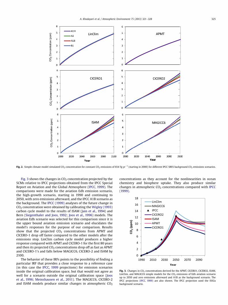
Fig. 2. Simple climate model simulated CO2 concentration for constant CO2 emissions of 654 Tg yr�1 (starting in 2000) for different IPCC SRES background CO2 emissions scenarios.

Fig. 3. Changes in CO2 concentrations derived for the APMT, CICERO1, CICERO2, ISAM,LinClim, and MAGICC6 simple models for the CO2 emissions of Edh aviation scenarioup to 2050 and zero emissions afterward and A1B as the background scenario. TheIPCC projections (IPCC, 1999) are also shown. The IPCC projection used the IS92abackground scenario.

A. Khodayari et al. / Atmospheric Environment 75 (2013) 321e328 325

Fig. 3 shows the changes in CO2 concentration projected by theSCMs relative to IPCC projections obtained from the IPCC SpecialReport on Aviation and the Global Atmosphere (IPCC, 1999). Thecomparisons were made for the aviation Edh emission scenario,the high-growth scenario, starting in 1990 and continuing to2050, with zero emissions afterward, and the IPCC A1B scenario asthe background. The IPCC (1999) analyses of the future change inCO2 concentration were obtained by calibrating the Wigley (1993)carbon cycle model to the results of ISAM (Jain et al., 1994) andBern (Siegenthaler and Joos, 1992; Joos et al., 1996) models. Theaviation Edh scenario was selected for this comparison since it isthe upper bound aviation emission scenario and elucidates themodel’s responses for the purpose of our comparison. Resultsshow that the projected CO2 concentrations from APMT andCICERO-1 drop off faster compared to the other models after theemissions stop. LinClim carbon cycle model produces a higherresponse compared with APMT and CICERO-1 for the first 80 yearsand then its projected CO2 concentrations drop off as fast as APMTand CICERO-1’s and falls below MAGICC6, CICERO-2 and ISAM by2100.

The behavior of these IRFs points to the possibility of finding aparticular IRF that provides a close response to a reference case(in this case the IPCC, 1999 projections) for emission scenariosinside the original calibration space, but that would not agree aswell for a scenario outside the original calibration space (Jooset al., 1996; Meinshausen et al., 2011). The MAGICC6, CICERO-2and ISAM models produce similar changes in atmospheric CO2

concentrations as they account for the nonlinearities in oceanchemistry and biosphere uptake. They also produce similarchanges in atmospheric CO2 concentrations compared with IPCC(1999).

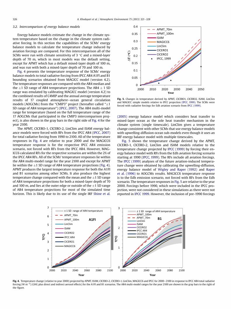
Fig. 5. Changes in temperature derived by APMT, CICERO1, CICERO2, ISAM, LinClimand MAGICC simple models relative to IPCC projection (IPCC, 1999). The SCMs wereforced with radiative forcings for Edh aviation scenario from IPCC (1999).

A. Khodayari et al. / Atmospheric Environment 75 (2013) 321e328326

3.2. Intercomparison of energy balance models

Energy balance models estimate the change in the climate sys-tem temperature based on the change in the climate system radi-ative forcing. In this section the capabilities of the SCMs’ energybalance models to calculate the temperature change induced byaviation forcings are compared. For this intercomparison all of theSCMs were run with climate sensitivity of 3 �C and a mixed-layerdepth of 70 m, which in most models was the default setting,except for APMT which has a default mixed-layer depth of 100 m,and was run with both a mixed-layer depth of 70 and 100 m.

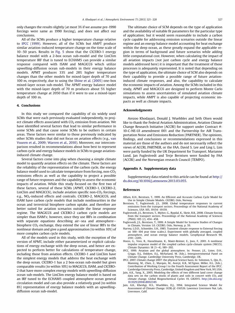
Fig. 4 presents the temperature response of the SCMs’ energybalancemodels to total radiative forcing from IPCC AR4 A1FI and B1bounding scenarios obtained from MAGICC model (version 4.2).The temperature responses are comparedwith the AR4median andthe �1 SD range of AR4 temperature projections. The AR4 � 1 SDrange was emulated by calibrating MAGICC model (version 4.2) tothe combined results of C4MIP and the annual average temperatureresults of 17 coupled atmosphereeocean general circulationmodels (AOGCMs) from the “CMIP3” project (hereafter called “�1SD range of AR4 temperature”) (IPCC, 2007). The AR4 multi-modelrange for temperature (based on the full temperature range of the17 AOGCMs that participated in the CMIP3 intercomparison proj-ect), is also shown in the gray bars in the right side of Fig. 4 for theyear 2100.

The APMT, CICERO-1, CICERO-2, LinClim and ISAM energy bal-ance models were forced with RFs from the IPCC AR4 (IPCC, 2007)for total radiative forcing from 1990 to 2100. All of the temperatureresponses in Fig. 4 are relative to year 2000 and the MAGICC6temperature response is for the respective IPCC AR4 emissionscenario, not forced with RFs from the IPCC AR4. However, MAG-ICC6 calculated RFs for the respective scenarios are within the 2% ofthe IPCC AR4 RFs. All of the SCMs’ temperature responses lie withinthe AR4 multi-model range for the year 2100 and except for APMTlie within the �1 SD range of AR4 temperature projections (Fig. 4).APMT produces the largest temperature response for both the A1FIand B1 scenarios among other SCMs. It also produce the highesttemperature change compared with the mean and the �1 SD rangeof AR4 temperature projections for both a mixed-layer depth of 70and 100 m, and lies at the outer edge or outside of the �1 SD rangeof AR4 temperature projections for most of the simulated timehorizon. This is likely due to its use of the single IRF Shine et al.

Fig. 4. Temperature change (relative to year 2000) projected by APMT, ISAM, CICERO-2, CICEforcing (W m�2) (GHG plus direct and indirect aerosol effects) for the A1FI and B1 scenarios.the figure.

(2005) energy balance model which considers heat transfer tomixed-layer ocean as the sole heat transfer mechanism in theclimate system (single timescale). LinClim gives a temperaturechange consistent with other SCMs that use energy balance modelswith upwelling-diffusion ocean sub-models even though it uses anIRF energy balance model with multiple timescales.

Fig. 5 shows the temperature change derived by the APMT,CICERO-1, CICERO-2, LinClim and ISAM models relative to thetemperature change projected by IPCC (1999) by forcing their en-ergy balance model with RFs from the Edh aviation forcing scenariostarting at 1990 (IPCC, 1999). The RFs include all aviation forcings.The IPCC (1999) analyses of the future aviation-induced tempera-ture change were obtained by calibrating the upwelling-diffusion,energy balance model of Wigley and Raper (1992) and Raperet al. (1996) to AOGCMs results. MAGICC6 temperature responseis to the Edh emission scenario, not forced with RFs from the Edhscenario. The temperature responses in Fig. 5 are relative to the year2000. Forcings before 1990, which were included in the IPCC pro-jection, were not considered in these simulations as there were notreported in IPCC 1999. However, the inclusion of pre-1990 forcings

RO-1, LinClim, MAGICC6 and IPCC for 2000e2100 in response to IPCC AR4 total radiativeThe AR4 multi-model ranges for the year 2100 are shown in the gray bars to the right of

A. Khodayari et al. / Atmospheric Environment 75 (2013) 321e328 327

only changes the results slightly (at most 3% if we assume pre-1990forcings were same as 1990 forcing), and does not affect ourconclusions.

All of the SCMs produce a higher temperature change relativeto IPCC (1999). However, all of the SCMs but AMPT producesimilar aviation-induced temperature change on the time scale of10e50 years. Results in Fig. 5 show that the CICERO-1 energybalance model with a 2-box ocean sub-model and the LinClimtemperature IRF that is tuned to ECHAM5 can provide a similarresponse compared with ISAM and MAGICC6 which utilizeupwelling-diffusion ocean sub-models in their energy balancemodels. APMT produces 33% and 28% higher temperaturechanges than the other models for mixed-layer depth of 70 and100 m, respectively, due to using the Shine et al. (2005) one-boxmixed-layer ocean sub-model. The APMT energy balance modelwith the mixed-layer depth of 70 m produces about 5% highertemperature change at 2050 than if it were to use a mixed-layerdepth of 100 m.

4. Conclusions

In this study we compared the capability of six widely usedSCMs that were each previously evaluated independently, to proj-ect climate effects associated with CO2 emission from aviation. Wehave identified several factors that lead to similar performance insome SCMs and that cause some SCMs to be outliers in certainareas. These factors were similar to those previously indicated byother SCMs studies that did not focus on aviation effects (e.g., vanVuuren et al., 2009; Warren et al., 2010). Moreover, our intercom-parison resulted in recommendations about how best to representcarbon cycle and energy balance models in SCMs to gauge aviation-induced climate change.

Several factors come into play when choosing a simple climatemodel to quantify aviation effects on the climate. These factors arethe reliability of the representation of the carbon cycle, the energybalancemodel used to calculate temperature from forcing, non-CO2emissions effects as well as the capability to project a possiblerange of future responses and the capability to assess the economicimpacts of aviation. While this study focused on the first two ofthese factors, several of these SCMs (APMT, CICERO-1, CICERO-2,LinClim and MAGICC6), include aviation specific non-CO2 forcings,e.g., NOx-induced effects and contrails. CICERO-2, MAGICC6, andISAM have carbon cycle models that include nonlinearities in theocean and terrestrial biosphere carbon uptake, and therefore arebetter suited for aviation scenarios outside the linear responseregime. The MAGICC6 and CICERO-2 carbon cycle models aresimpler than ISAM’s; however, since they use IRFs in combinationwith separate equations describing airesea and atmosphereebiosphere CO2 exchange, they extend the use of linear IRFs to thenonlinear domain and give a good approximation (towithin 10%) ofmore complex carbon cycle models.

All of the models used in this study, with the exception of theversion of APMT, include either parameterized or explicit calcula-tions of energy exchange with the deep ocean, and hence are ex-pected to perform better for calculations of temperature change,including those from aviation effects. CICERO-1 and LinClim havethe simplest energy models that address the heat exchange withthe deep ocean. CICERO-1 has a 2 box-ocean sub-model but givescomparable results (to within 10%) to MAGICC6, ISAM, and CICERO-2 that have more complex energy models with upwelling-diffusionocean sub-models. The LinClim energy balance model is based onan IRF tuned to the ECHAM5 coupled atmosphere ocean generalcirculation model and can also provide a relatively good (to within8%) representation of energy balance models with an upwelling-diffusion ocean sub-model.

The ultimate choice of SCM depends on the type of applicationand the availability of suitable fit parameters for the particular typeof application; but it would seem reasonable to include a carboncycle capable for addressing emission scenarios outside the linearregime and an energy balance model accounting for heat exchangewithin the deep ocean, as these greatly expand the applicable re-gion in terms of background and future scenarios while addinglittle computational cost. However, when calculating the impact ofall aviation impacts (not just carbon cycle and energy balancemodels addressed here) it is important that the treatment of thoseprocesses is adequately represented. It is noted that depending onthe type of application, the ultimate choice of SCM also depends ontheir capability to provide a possible range of future aviation-induced climate responses, and also, the capability to calculatethe economic impacts of aviation. Among the SCMs included in thisstudy, APMT and MAGICC6 are designed to perform Monte Carlosimulations to assess uncertainties of simulated aviation climateimpacts, while AMPT is also capable of projecting economic im-pacts as well as climate impacts.

Acknowledgments

Arezoo Khodayari, Donald J. Wuebbles and Seth Olsen wouldlike to thank the Federal Aviation Administration, Aviation ClimateChange Research Initiative (ACCRI) for support under Contract #:10-C-NE-UI amendment 001 and the Partnership for AiR Trans-portation Noise and Emissions Reduction (PARTNER). The opinions,findings, and conclusions or recommendations expressed in thismaterial are those of the authors and do not necessarily reflect theviews of ACCRI, PARTNER, or the FAA. David S. Lee and Ling L. Limwere partly funded by the UK Department for Transport. MarianneLund, Jan Fuglestvedt and Terje Berntsen were funded by FAA(ACCRI) and the Norwegian research Council (TEMPO).

Appendix A. Supplementary data

Supplementary data related to this article can be found at http://dx.doi.org/10.1016/j.atmosenv.2013.03.055.

References

Alfsen, K.H., Berntsen, T., 1999. An Efficient and Accurate Carbon Cycle Model forUse in Simple Climate Models. CICERO, Oslo, Norway.

Berntsen, T., Fuglestvedt, J.S., 2008. Global temperature responses to currentemissions from the transport sectors. Proceedings of the National Academy ofSciences, USA 105, 19154e19159.

Fuglestvedt, J.S., Berntsen, T., Myhre, G., Rypdal, K., Skeie, R.B., 2008. Climate forcingfrom the transport sectors. Proceedings of the National Academy of Sciences(PNAS) 105 (2), 454e458.

Fuglesvedt, J.S., Berntsen, T., 1999. A Simple Model for Scenario Studies of Changesin Climate, Version 1.0. CICERO, Oslo, Norway, p. 59.

Harvey, L.D.D., Schneider, S.H., 1985. Transient climate response to External forcingon 100e104 year time scales,1. Experiment with globally averaged, coupledatmosphere, and ocean energy balance models. Geophysical Research 90,2191e2205.

Hooss, G., Voss, R., Hasselmann, K., Maier-Reimer, E., Joos, F., 2001. A nonlinearimpulse response model of the coupled carbon cycle-climate system (NICCS).Climate Dynamics 18 (3e4), 189e202.

IPCC, 1999. Aviation and the global atmosphere. In: Penner, J.E., Lister, D.H.,Griggs, D.J., Dokken, D.J., McFarland, M. (Eds.), Intergovernmental Panel onClimate Change. Cambridge University Press, Cambridge, UK.

IPCC, 2007. Climate change 2007: the physical Science basis. In: Solomon, S., Qin, D.,Manning, M., Chen, Z., Marquis, M., Averyt, K.B., M.Tignor, Miller, H.L. (Eds.),Contribution of Working Group I to the Fourth Assessment Report of the IPCC.CambridgeUniversity Press, Cambridge, United KingdomandNewYork, NY, USA.

Jain, A.K., Yang, X., 2005. Modeling the effects of two different land cover changedata sets on the carbon stocks of plants and soils in concert with CO2 andclimate change. Global Biogeochemical Cycles 19, GB2015. http://dx.doi.org/10.1029/2004GB002349.

Jain, A.K., Kheshgi, H.S., Wuebbles, D.J., 1994. Integrated Science Model forAssessment of Climate Change. UCRL-JC-116526. Lawrence Livermore Nat. Lab,Livermore, Calif.

A. Khodayari et al. / Atmospheric Environment 75 (2013) 321e328328

Joos, F., Bruno, M., Fink, R., Stocker, T.F., Siegenthaler, U., LeQuéré, C., Sarmiento, J.L.,1996. An efficient and accurate representation of complex oceanic andbiospheric models for anthropogenic carbon uptake. Tellus 48B, 397e417.

Joos, F., Prentice, I.C., Sitch, S., Meyer, R., Hooss, G., Plattner, G.K., Gerber, S.,Hasselmann, K., 2001. Global warming feedbacks on terrestrial carbon uptakeunder the IPCC emission scenarios. Global Biogeochemical Cycles 15, 891e907.

Lee,D.S., Fahey,D.W., Forster, P.M.,Newton, P.J.,Wit,R.C.N., Lim, L.L.,Owen, B., Sausen, R.,2009. Aviation and global climate change in the 21st century. AtmosphericEnvironment 43, 3520e3537. http://dx.doi.org/10.1016/j.atmosenv.2009.04.024.

Li, S., Jarvis, A.J., Leedal, D., 2009. Are response function representations of theglobal carbon cycle ever interpretable? Tellus 61B, 361e371.

Lim, L.L., Lee, D.S., Sausen, R., Ponater, M., 2006. Quantifying the effects of aviationon radiative forcing and temperature with a climate response model. In: Pro-ceedings of an International Conference on Transport, Atmosphere and Climate(TAC). Office for Official Publications of the European Communities,Luxembourg, pp. 202e207.

Marais, K., Lukachko, S.P., Jun, M., Mahashabde, A., Waitz, I.A., 2008. Assessing theimpact of aviation on climate. Meteorologische Zeitschrift 17 (2), 157e172.

Marten, A.L., 2011. Transient Temperature Response Modeling in IAMs: the Effectsof Over Simplification on the SCC. Economics: Discussion Papers, No 2011-11.Kiel Institute for the World Economy. http://www.economics-ejournal.org/.

McCarthy, J., 2010. Aviation and climate change. In: Blumenthal, G. (Ed.), Aviationand Climate Change. Nova Science Publishers, Inc., USA.

Meinshausen, M., Raper, S.C.B., Wigley, T.M.L., 2011. Emulating coupled atmos-phereeocean and carbon cycle models with a simpler model, MAGICC6 e part1: model description and calibration. Atmospheric Chemistry and Physics 11,1417e1456. http://dx.doi.org/10.5194/acp-11-1417.

Raper, S.C.B., Wigley, T.M.L., Warrick, R.A., 1996. Global sea level rise: past andfuture. In: Milliman, J., Haq, B.U. (Eds.), Sea-level Rise and Coastal Subsidence:Causes, Consequences and Strategies. Kluwer Academic, pp. 11e45.

Roeckner, E., Baeuml, G., Bonventura, L., Brokopf, R., Esch, M., Giorgetta, M.,Hagemann, S., Kirchner, I., Kornblueh, L., Manzini, E., Rhodin, A., Schlese, U.,Schulzweida, U., Tompkins, A., 2003. The Atmospheric General CirculationModel ECHAM5. PART I: Model Description. Report 349. Max Planck Institutefor Meteorology, Hamburg, Germany.

Schlesinger, M.E., Jiang, X., Charlson, R.J., 1992. Implications of AnthropogenicAtmospheric Sulphate for the Sensitivity of the Climate System, ReprintedForm Climate Change and Energy Policy. American Institute of Physics, NewYork.

Shine, K.P., Fuglestvedt, J.S., Hailemariam, K., Stuber, N., 2005. Alternatives to theglobal warming potential for comparing climate impacts of emissions ofgreenhouse gases. Climatic Change 68 (3), 281e302. http://dx.doi.org/10.1007/s10584-005-1146-9.

Siegenthaler, U., Joos, F., 1992. Use of a simple model for studying oceanic tracerdistributions and the global carbon cycle. Tellus 44B, 186e207.

Thompson, M.V., Randerson, J.T., 1999. Impulse response functions of terrestrialcycle models: method and application. Global Change Biology 5, 371e394.

van Vuuren, D.P., Lowe, J., Stehfest, E., Gohar, L., Hof, A.F., Hope, C., Warren, R.,Meinshausen, M., Plattner, G.K., 2009. How well do integrated assessmentmodels simulate climate change? Climatic Change http://dx.doi.org/10.1007/s10584-009-9764-2.

Warren, R., Mastrandrea, M., Hope, C., Hof, A., 2010. Variation in the climaticresponse to SRES emissions scenarios in integrated assessment models. Cli-matic Change 102 (3), 671e685. http://dx.doi.org/10.1007/s10584-009-9769-x.

Wigley, T.M.L., 1993. Balancing the carbon budget: implications for projections offuture carbon dioxide concentration changes. Tellus 45B, 409e425.

Wigley, T.M.L., Raper, S.C.B., 1992. Implications for climate and sea level of revisedIPCC emissions scenarios. Nature 357, 293e300.

Wigley, T.M.L., Raper, S.C.B., 2001. Interpretation of high projections for global-mean warming. Science 293, 451e454.