interaction between beam control and rf feedback...

Interaction Between Beam Control and RF Feedback

Loops for High Q Cavities and Heavy Beam Loading

Superconducting Super Collider Laboratory

SSCL-Preprint-195 February 1993 Distribution Category: 414

L.K. Mestha C.M.Kwan K.S. Yeung

SSCL-Preprint-195

Interaction Between Beam Control and RF Feedback Loops for High Q Cavities and Heavy Beam Loading*

L.K. Mestha and C.M. Kwan

Superconducting Super Collider Laboratory t 2550 Beckleymeade Ave.

Dallas, TX 75237

K.S. Yeung

University of Texas Arlington, TX 76019

February 1993

·To be submitted to the "Particle Accelerators Journal."

tOperated by the Universities Research Association. Inc .• for the U.S. Department of Energy under Contract No. DE-AC35-89ER40486.

*

INTERACTION BETWEEN BEAM CONTROL AND RF FEEDBACK LOOPS FOR HIGH Q CAVITIES

AND HEAVY BEAM LOADING

L. K. MESTHA AND C.M. KWAN

Superconducting Super Collider Laboratory, * Dallas, Texas 75237

K.S. YEUNG

University of Texas, Arlington, Texas 76019

An open-loop state space model of all the major low-level rf feedback control

loops is derived. The model has control and state variables for fast-cycling machines

to apply modern multi variable feedback techniques. A condition is derived to know

when exactly we can cross the boundaries between time-varying and time-invariant

approaches for a fast-cycling machine like the Low Energy Booster (LEB). The

conditions are dependent on the Q of the cavity and the rate at which the frequency

changes with time. Apart from capturing the time-variant characteristics, the errors

in the magnetic field are accounted in the model to study the effects on

synchronization with the Medium Energy Booster (MEB). The control model is

useful to study the effects on beam control due to heavy beam loading at high

intensities, voltage transients just after injection especially due to time-varying

voltages, instability thresholds created by the cavity tuning feedback system, cross

coupling between feedback loops with and without direct rf feedback etc. As a

special case we have shown that the model agrees with the well known Pedersen

model derived for the CERN PS booster. As an application of the model we

undertook a detailed study of the cross coupling between the loops by considering all

of them at once for varying time, Q and beam intensities. A discussion of the method

to identify the coupling is shown. At the end a summary of the identified loop

interactions is presented.

Operated by Universities Research Association, Inc., for the U.S. Department of Energy under Contract No. DE-AC35-89ER40486.

1 INTRODUCTION

There are several feedback loops associated with the complete low-level rf system. There are

high-bandwidth cavity amplitude and phase loops and a low-bandwidth tuning loop all of them

local to the cavity. The radial loop, beam phase loop and synchronization loop are global to the

ring accelerating system. For high-Q rf cavities the high-bandwidth local phase loop and

amplitude loops may interact with the beam phase loop. It is a general practice in the

accelerator community to design these loops as though there is only one loop acting on the

machine in isolation and then collectively put them together to operate the machine with beam.

It may so happen that the control signal from the local cavity phase loop has a significant effect

on the beam phase which in effect may act against the function of the beam phase loop.

Similarly, the control from the cavity amplitude loop may effect the beam phase loop at some

frequencies below or above synchrotron frequencies. These effects are hard to see when all the

loops are combined. Also, the loop interactions may be dominant when a high-Q cavity system

is used to operate the machine at high intensities. Our aim in this paper is to show a method to

identify the loop interactions on a highly-coupled system like the Low Energy Booster

RF system and then, later in the paper, discuss the effects due to variable Q (by including direct

rf feedback) and variable beam intensities. Also, we discuss several methods to decouple the

loops so that eventually each loop can be designed as single loop.

To study a coupled system, a good mathematical model of the beam feedback system with

cavity dynamics is extremely useful. Otherwise, we have to rely on the measurement data on an

operating machine which becomes virtually difficult to acquire on a time-varying machine.

The complete analytical system model gives information such as the open-loop bandwidth,

gain and phase values at different frequencies for each loop. Especially, a state-space model is

better since the additional disturbance terms which are the functions of the cavity and machine

parameters can be observed and compensated in the loops. In the literature we see work related

to the development of a transfer function model by Pedersen 1 in the 1970s and subsequently by

other authors.2,3 We see that a control model for fast-cycling machines was not obtained to

integrate all the loops including the local phase loop planned for the Low Energy

2

Booster (LEB). In the initial stages of this paper an open-loop state-space model of the control

loops is derived. Our model has all control and state variables for fast-cycling machines to

apply modem multi variable feedback techniques. As a special case the model is compared with

Pedersen's model for a time-invariant machine. After deriving the model we show the

normalization techniques and then the coupled transfer characteristics with respect to

frequency at a given time during acceleration for conditions with direct rf feedback and then for

varying beam currents. The information will be useful to design a complete decoupled

low-level rf system.

2 DESCRIPTION OF THE LEB RF BEAM CONTROL LOOPS

Several feedback loops are associated with the complete low-level rfsystem. The goal of the

system is to be able to bunch the beam, accelerate and extract to the higher-energy machine. To

be able to do this a precise control of the frequency, phase, and amplitude of the gap voltage is

required. In Figure 1 we show the complete feedback loops associated with the LEB with two

cavities to represent the signal distribution. Loops can be divided based on their functions.

Loops local to each of the rf stations are called local cavity loops in this paper. Also, those loops

controlling the frequency of the drive rf signal by sensing the beam information are called

global loops.

2.1 Feedback Loops Local to Each Cavity

There are four feedback loops shown local to each cavity: a direct rf feedback loop, a cavity

tuning loop, a local phase loop, and a local amplitude loop. The direct rf feedback loop consists

of summing the processed gap voltage signal with the signal before the power amplifier as

shown in Figure 1. This loop has the effect to reduce the effective Q of the cavity. 1 The local

phase loop in essence consists of a phase detector (PD), a feedback controller, and a phase

shifter CPS). The phase detector measures the phase difference between the rf signal supplied

from the global frequency control unit and the measured gap voltage. The phase loop operates

by changing the phase of the generator current at the rf signal frequency driving the power

amplifier. It is included to maintain the cavity gap voltage at the phase set by the rf drive signal

3

from the global frequency control unit. The local amplitude loop changes the amplitude of the

generator current to maintain the error between the envelope of the gap voltage signal and the

reference voltage signal to within specification. Thus, the local amplitude loop maintains the

required amplitude on the gap voltage signal. Both amplitude and phase loops are particularly

more effective at high beam intensities. The open-loop bandwidths of these loops are important

and depend on the cavity and machine parameters. The cavity tuning loop, on the other hand, is

isolated from the amplitude and phase loops. It consists of a phase detector to measure the

phase difference due to tuning error. This signal is fed to the Tuning Bias Regulator (TBR)

through a controller driving the ferrite tuner to correct for the tuning error. The set point is

required to add a detuning profile after the beam is injected into the machine. It also helps for

arranging additional feedforward correction needed for the tuning loop. The tuning loop is

generally slow due to the cost involved in building fast tuners.

2.2 Feedback Loops Global to the Cavity

The global feedback loops have the special task of controlling the beam to capture and

accelerate while correcting for radial excursions due to field errors. The synchronization of the

beam bunches from the LEB to the MEB is another requirement. The global loops are: radial .

loop, beam phase loop, and synchronization loop. Interconnection of these loops is shown in

Figure 1. A stable frequency source such as the Direct Digital Synthesizer (DDS) is used for

producing a sinusoidal rf signal by way of reading frequency ramp values from a table. The

frequency ramp table is inexorable and needs corrections to minimize errors in beam orbit or

coherent beam oscillations around the synchronous phase. In the radial loop, the radial position

of the beam is compared to a preset steering reference signal to generate the radial error signal.

The radial error signal is processed and then the resulting signal adds or subtracts the frequency

ramp values to maintain the radial error to within the specifications. In the beam phase loop, the

beam position signal is compared directly from a wall-current monitor in the beam phase

detector. It is then processed to convert to the appropriate frequency shift through a feedback

controller. The frequency shift is added to the frequency ramp values. The synchronization

loop is configured depending on the approach needed. In the trip-plan scheme,4 the time

4

interval between the LEB and the target MEB markers is measured preferably using a . Time-to-Digital Converter (TDC) at the time the target MEB marker appears. The data is then

compared with a table and processed to generate the frequency shift to the ramp values. In this

way locking can be achieved to predetermined values so that the synchronism is guaranteed. In

addition to the loops we have described, there could be loops to damp the quadrupole

oscillations. Also, one-tum delay loops to correct the effects on cavities due to gaps in the

machine are commonly used in many accelerators. The global paraphase hardware, as shown

in Figure 1, is also used to maintain low effective gap voltage at the time of injection.

All the active loops are important for the operation of the machine. Their design is highly

complex and it becomes even more complicated when some of the loops are coupled. To ensure

global stability of the loops and also meet the specifications on gap voltage phase and

amplitude, it will be useful to know the coupling between them. The 'coupling' means: say for

example, the control of a local phase loop (phase shift of the rf drive signal in the local

rf station) affecting the beam phase error or vice versa. Such things are very hard to see unless a

complete system model is derived. Especially, a state-space model is better since the additional

disturbance terms which are the functions of the cavity and machine parameters can be

observed and compensated in the loops. We have, therefore, actively pursued a rigorous

mathematical approach in deriving the control model which is shown below.

3 GLOBAL AND LOCAL CONTROL MODEL

At first, a general control model to include all the feedback loops is derived by using an

equivalent circuit model for the cavity. Later, we show a simplified reduced order model in

analytical form. Comparisons are made with a special particle tracking code developed at the

Superconducting Super Collider Laboratory (SSCL) to test the validity of the model.

3.1 Cavity Control Model

Consider a parallel equivalent RLC circuit for the cavity (Figure 2). Then the following

differential equation can be written for the total gap voltage, v, with CJ)R as the resonant

frequency.

5

where

d v dv 2 ooR d R ooRV dR It 2 [ 3 Q ] d' -+20-+00 - ---(--)!vdt+-- ... 20Rdr dt R R dt ooRQ RQ dt dt

o = = Damping ratio

(1)

The terms within the square bracket have resulted during simplification of the RLC equivalent

circuit model due to time-varying frequency. For the parameters of the LEB, this term can be

ignored. Hence we use the following simplified model

v + 20v + oo~v ... 20Rit • (2)

The gap voltage, v, generator current ig and the beam current ib can be represented in terms of

their fundamental components as below

v (t) ifoodt

- Vle

ig (t) ifoodt

- Igle (3)

ib (t) ifoodt

.. Ible .

The amplitudes VI> IgI and Ibl respectively for the gap voltage, generator current and beam

current will be regarded as phasors in the analysis to follow. The term, ej f wdt, represents the

phase due to frequency of the driving rfpower which is time varying in fast-cycling machines.

Generally, for studies related to beam loading instabilities, the exponent term, eP»t, was used in

the literature.2 This representation is valid, when the frequency of the rf signal is not varying

with time to see significant differences in the stability of the feedback loops. However, for

studies related to global stability of the loops from injection, throughout acceleration and until

extraction we need to use a more accurate representation of the model since the frequency

6

begins to ramp at a considerably faster rate for the LEB. In Appendix A, we derive three simple . inequalities to show when actually the phase is represented with the exponent having the

integral term. One of the inequalities, ~ ~ cg;, is not satisfied for the LEB. Hence the

representation shown in Eq. (3) is more accurate for the LEB.

3.1.1 Cavity Voltage and P hase Model. The formulation of the voltage and current phasors

shown in Eq. (3) leads to an accurate control model which is different from that shown in the

literature2 due to the time-varying nature of the frequency. To determine the representation of

the amplitudes VI, Ig I and Ib I in Eq. (3) we need to identify the measurable signals and control

signals used for all the feedback loops around the cavity. Figure 3 shows the line diagram of the

loop interface points of Figure 1. The "controller" of Figure 3 can be modeled with a simple

gain or modeled with additionallinear/nonlinear dynamics. The measured quantities (without

any superscript) are shown symbolically pointing to the controller of each loop and the control

parameters are shown with a superscript 'c'. Also the direct rf feedback is represented with a

feedback gain of ~. By assuming the power amplifier as a high-bandwidth system with a pure

gain of Kg, we can rewrite the equation for the generator current as follows

, ig == (ig-Kdv)Kg , (4)

where ig is the rf signal derived after applying appropriate frequency, amplitude, and phase

correction from the local and global feedback loops. Substituting Eq. (4) into (1) we obtain

(5)

where

(6)

(7)

7

Whereas with direct-rf feedback the generator current becomes, ig = (HlKg )ig and the

steady-state generator current Ig = H(VIRKg) for the case without beam loading compensation.

R is the equivalent shunt resistance of one cavity and Kg is the equivalent gain of the power

amplifier driving one accelerating cavity. Clearly, the increase in the loop gain in the direct rf

feedback loop and the power amplifier gain have a direct effect in reducing the effective Q of

the cavity. The generator current, ig can be regarded as the rf signal which will be combined

with the direct rf feedback loop to generate the new rf signal driving the power amplifier. It

must be noted at this stage that with the presence of direct rf feedback the generator current, ig ,

at the summing point is increased by the factor H.

In Figure 4, a phasor diagram is shown to represent the relations among the currents and

voltages at a given time for the machine operating at below transition. Under steady-state

conditions the phase between the cavity gap voltage and the generator current is equal

to $ L-the loading phase angle (1) which is equal to the cavity impedance phase angle for no

beam. $z is the phase angle of the total current (generator current, ig + fundamental beam

current, I b) with respect to gap voltage. The phase b$v is the transient perturbation in the cavity

gap voltage acting as phase modulation over the steady-state voltage "ideal. A local phase loop

will maintain b<l>v to zero during normal operation. The phase modulation b<l>c is applied to the

steady-state generator current in the local phase loop to maintain b$v to zero. Since when the

beam comes on, the amplitude of the cavity voltage cbanges by b V, V = Videal + b V, by

modulating the amplitude of ig• b V is suppressed in the amplitude loop.

From Figure 3 it is clear that the generator current rf signal, ig , is phase and frequency

modulated by various feedback loops. Therefore, the dynamical representation of the

generator current, ig , is shown below in terms of the control parameters

(8)

Similarly, the fundamental of the beam current and the cavity gap voltage is represented as

follows

8

(9)

j (J( w + 6wc) dt + 6/j1)

v .. (V+()V)e . (10)

Where booc is the sum of all the frequency shifts in radians per second applied from the global

control loops as shown in Figure 3. Parameters of the tuning loop model will be included later.

The currents ig and lb are differentiated once with respect to time and the gap voltage is

differentiated twice with respect to time. The resulting derivatives of the current and voltage

phasors are substituted in the modified equivalent circuit Eq. (5) above. After some

simplification, real and imaginary parts are equated with those on the right-hand side. As a

result, the following two nonlinear equations are obtained:

where

11 - 20RKg { (ig + ()f) cos (ch + ()cpc - ()cp) -

. (Ig + ()f) (00 + ()ooc + ~L + ()r) sin (CPL + ()cpc - ()cpv) - s s - c· s . s s s

-Ibsin (()cpv + cp + ()cp ) + Ib (00 + ()oo -cp -()cp ) cos (()cpv + cp + ()cp ) },

12 - 20RKg { (ig + ()l) sin (CPL + ()cpc - ()cpv) + (13)

(Ig + ()f) (00 + ()ooc + ~L + ()~c) cos (CPL + ()cpc - ()cpv)

.; s s - c· s . s s s -Ibcos«()cpv+cp +()cp )-Ib(oo+()oo -cp -()cp ) sin «()cpv+ cp +()cp) },

-V .. V + {)V,

h - IblKg .

Equations (12) and (13) are second order and non-linear. They can be reduced to first-order

non-linear form by using the approximations shown below.

9

.. . - -V« 20HV

V6~v « 20H (00 + 60/) V and 20HV6~v

- .2 c - . V6cj> v« 2 (<.0 + 600 ) V6cj>v

2V6~v« 2 (<.0 + 600C) V

V(w+6ci/) «20H(00+600C )V .

The reduced order non-linear model becomes:

20HV - 2 (00 + 60{) V6~v + [ (<'oR + 6<'oR) 2 - (<.0 + 600c) 2J if .. 11 ,

c .; - . c -2 (<.0 + 600 ) V + 20HV6cj>v + 20H (<.0 + 6<.0 ) V - 12 .

(14)

(15)

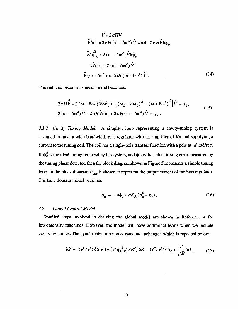
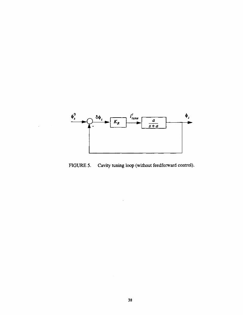
3.1.2 Cavity Tuning Model. A simplest loop representing a cavity-tuning system is

assumed to have a wide-bandwidth bias regulator with an amplifier of KR and supplying a

current to the tuning coil. The coil has a single-pole transfer function with a pole at 'a' rad/sec.

If ~ is the ideal tuning required by the system, and <Pz is the actual tuning error measured by

the tuning phase detector, then the block diagram shown in Figure 5 represents a simple tuning

loop. In the block diagram i~ne is shown to represent the output current of the bias regulator.

The time domain model becomes

(16)

3.2 Global Control Model

Detailed steps involved in deriving the global model are shown in Reference 4 for

low-intensity machines. However, the model will have additional terms when we include

cavity dynamics. The synchronization model remains unchanged which is repeated below.

(17)

10

Where 5S is the synchronization phase error, 5R is the average radial offset from the central

orbit, 5B is the magnetic field error from the ideal curve B, RS is the radius of the m/e, and V S is

the velocity of the synchronous particle. While deriving the model representing transverse

orbital deviations, the particle phase contains the nominal synchronous phase, phase

representing coherent dipole motion, O<j>s, and the phase shift O<j>v. The non-linear model is in

the form shown below

Where the coefficients A 1 and A 3 are defined later in Table I in this paper. Also the differential

equation for the synchrotron phase oscillations is modified by additional terms, which are the

derivatives of the phase shift and are shown below.

(19)

3.3 Linear State Space Model

Since most of the signals are small, we can derive a control model by linearizing Eqs. (15)

through (19). While linearizing Eq. (15) the following approximations are used.

cos (6cpc - 6cpv) - 1

sin (6cpc - 6cpv) - 6cpc - 6cpv

cos ( 6 cps + 6cp) - 1

.C 6<1> «w

.C

6cp - 0

11

(20)

The products of small quantities such as 6ooc6 V, 6 V6$v etc., are ignored. The tuning angle <Pz . is introduced 1 as below by assuming 600 R = 600c

(21)

From the vector diagram, under steady-state conditions the following equations hold good.

IgCOS(h - 10 (1 + Ysinq,S)

ibcosq,s .. Igsinq,L + lotanq,~

1 + Ysinq,s

VB 10 .. RK ;

g

(22)

Note that the direct rf feedback (term H) reduces the beam loading term, Y. After linearizing

Eq. (15) and substituting the approximations, we get the state space equations in the form

shown in Table I, which follows Appendix B.

4 MODEL VALIDATION TESTS

Once the model is constructed for the control system in hand, it is logical to test the model to

compare with some known quantities. Pedersen derived a transfer function model for some of

the fast loops for a non-time-varying machine. In Appendix B we show the derivation of the

Pedersen model from the equations shown in Table I as a special case to confirm the validity of

the matrices and satisfy Robinson's stability criteria. A more appropriate comparison is to use

the longitudinal particle tracking code and compare the states to those obtained by integrating

the model. In this way, we would have made the direct comparison of the model for the

time-varying conditions. The longitudinal tracking code was developed by us with a lumped

cavity which is represented in the form of an equivalent circuit. We show in Reference 5 the

description of the tracking code with the cavity model and special measurement techniques to

extract the beam phase.

12

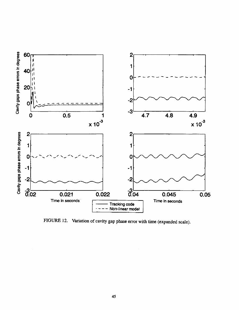
In Figures 6 through 12 the radial position, beam phase error, cavity amplitude error, and \

cavity phase errors are plotted against time for up to 50 milliseconds with all the loops opened.

The solid lines represent the simulated results using the longitudinal tracking code with a

discrete time of about 4000 units-per-one rf period. The dashed lines are obtained by using the

non-linear global and local models, Eqs. (15) to (19). To create synchrotron oscillations we

injected a particle with a lOMe V injection error from the Linac to the LEB and tracked a single

particle up to 50 ms. A cavity with a Q of 5000 was used. A linear model would not be practical

for large amplitude oscillations of over 40 degrees beam phase error, hence the comparison is

not shown. In conclusion, the model predicts the essential dynamics of the particle.

The cavity voltage error, 0 V, has very high initial transients when there is no feedback as

shown in Figure 11 for first 1 ms after injection. This transient has been identified to be due to

the high rate of change of voltage at the beginning, just after injection. In the state-space

equation of Table I we have shown terms such as C4 and C5. They are zero in Pedersen's model

due to no direct rf feedback term (H = 1) and no time varying terms (V = 0). The direct

rf feedback reduces the initial voltage transient on the gap, but is found to be insufficient. In

theory the amplitude and phase loops must be able to reduce the transient to zero, but this is

restricted by the overall stability limits and the cavity tuning conditions. Using the state-space

model and special compensation techniques we can control the voltage transients to within

specifications. Detailed study on this topic is a subject for another paper and will be pursued in

the future. In the discussion to follow special techniques are shown to investigate the

interaction between loops.

5 COUPLED TRANSFER FUNCTIONS

The linear state-space model is a good start to study the coupled transfer characteristics.

Since our control problem is multi-variable, at first we have to realize a state-space description

for a mUlti-input multi-output case. To proceed, let us consider the model of Table I in terms of

system matrix A and input matrix B as follows:

13

(23)

where :!represents the states and Hrepresents various control signals. The additional term 4is a

disturbance matrix with parameters shown in Table I. The disturbance matrix has important

concern with regard to controlling the beam for time-varying machines which will not be

discussed in this paper. For studying coupled transfer characteristics we ignore the disturbance

matrix.

Consider the output matrix l: defined such that it satisfies

(24)

where C is an identity matrix. The outputs are defined by the above equation.

Taking Laplace Transform of Eqs. (23) and (24), the following equation can be obtained

Yes) ... C (sl-A)-l/ly

-=Q(s)y. (25)

The matrix G(s) is an open-loop transfer matrix defined between the control inputs and the

outputs. It is given by

Q(s) - (26)

14

The components of the open loop transfer matrices G( s) are shown below in terms of the known

measured quantities and the control parameters. They are:

Gu (s) -Xl (s) L\S (s)

G21 (s) .. X 2 (s) L\R(s)

U I (s) L\pc (s) U I (s) L\pc (s)

Gl2 (s) .. Xl (s) L\S (s)

G22 (s) ... X 2 (s) L\R(s)

U2 (s) L\pc (s) U 2 (s) L\pc (s)

G13 (s) Xl (s) L\S (s)

G23 (s) .. X 2 (s) L\R(s)

= U3 (s) MC(s) U 3 (s) L\pc (s)

Gl4 (s) -Xl (s) L\S (s)

G24 (s) .. X 2 (s) L\R(s)

U4 (s) M(s) U4 (s) M(s)

GIS (s) ... Xl (s) L\S (s)

G25 (s) .. X 2 (s) L\R(s)

Us (s) L\cj/ (s) Us (s) L\cj/ (s)

G l6 (s) -Xl (s) L\S (s)

G26 (s) .. X 2 (s) L\R(s)

U6 (s) ~une (s) U6 (s) ~une (s)

15

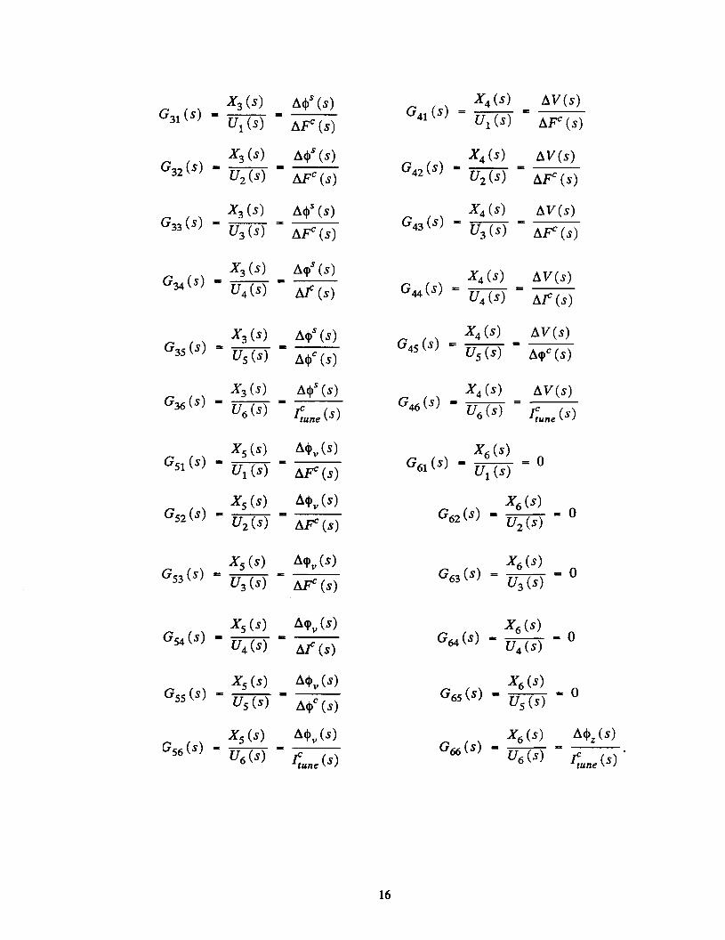
X3 (s) ~s (s) G 41 (s)

X4 (s) ~V(s) G31 (s) =

U1 (s) ~Fc (s) U1 (s) ~Fc (s)

G32 (s) -X3 (s) ~s (s)

G42 (s) -X4 (s) ~V(s)

U2 (s) - U2 (s) MC(s) ~Fc (s)

X3 (s) ~s (s) G43 (s) -

X 4 (s) ~V(s) G33 (s) ...

U3 (s) ~Fc (s) U3 (s) ~Fc (s)

G34 (s) -X3 (s) ~s (s) X4 (s) ~V(s)

G44 (S) = U4 (S) M(s) = U4 (s) ~~(s)

X3 (s) ~s (s) G4S (s) ...

X4 (s) ~V(s) G3S (s) ... - ...

Us (s) ~c (s) Us (s) ~c (s)

G36 (s) ... X3 (s) ~s (s)

G46 (S) ... X4 (S) ~V(S)

U6 (S) t;une (s) U6 (s) t:une (s)

GS1 (S) -Xs (s) ~v (S) X6 (S)

U1 (s) ~pc (S) G 61 (S) ... U 1 (s) = 0

GS2 (S) -Xs (S) ~v(s)

G62 (S) X6 (s)

- 0 - U2 (S) U2 (s) ~pc (s)

GS3 (s) ... Xs (s) ~v (s)

G63 (s) X6 (S)

... 0 = U3 (s) U3 (s) MC(s)

GS4 (s) -Xs (s) ~v (s)

G64 (s) X6 (s)

U4 (s) - - - 0 M(s) U4 (s)

GSS (S) -Xs (s) ~v (s)

G6S (s) X6 (s)

.. 0 Us (s) ~c (s) - Us (s)

Xs (s) ~v (s) G66 (s)

X6 (s) ~z (s) GS6 (s) - - -U6 (s) t;une (s) U6 (s) t;une (s)

16

Gain curves of Eq. (26) show the coupling between different inputs and outputs. For

example, to study the effect on beam phase, (Y3 = X3), due to the simultaneous modulations on

(1) the frequency, fJ:f = u3' (2) the amplitude of the rf signal, MC = u4' and (3) the phase of

the rf signal, fJ<t>c = us' we plot gains G33(S), G34(S) and G3S(S) with respect to frequency.

However, to compare the amplitude of the gains, first they have to be normalized to a certain

index. We show below how to normalize the gain matrix. After this, the actual plots of the gains

are shown with respect to the modulating frequency for different control signals.

To normalize the open-loop transfer matrix, we first normalize the states and the controls.

The normalized state matrix is given by

i .. diag {1/~~} ~

.. Tx -x- i = 1, 2, ... , 6, (27)

where Ix is the diagonal transformation matrix for unnormalized states. The elements xi are

the maximum values of the measured states in the state matrix, :!. Similarly, the normalized

control matrix is given by

y - diag {1/!.l~} !.l

- T u -u- i = 1, 2, ... , 6, (28)

where Iu is the diagonal transformation matrix for unnormalized control quantities. The

elements ui are the maximum values of the control quantities. After substituting Eqs. (27)

and (28) in Eqs. (23) and (24) and converting the resulting equation to frequency domain we

get a new equation shown below

- - - -1 - -Yes) .. c (sl-~) OIl (s)

- -.. Q(s)I!(s) , (29)

where

c .. cr1 - --x

The normalized gain matrix, (;(s), is now dimensionless.

17

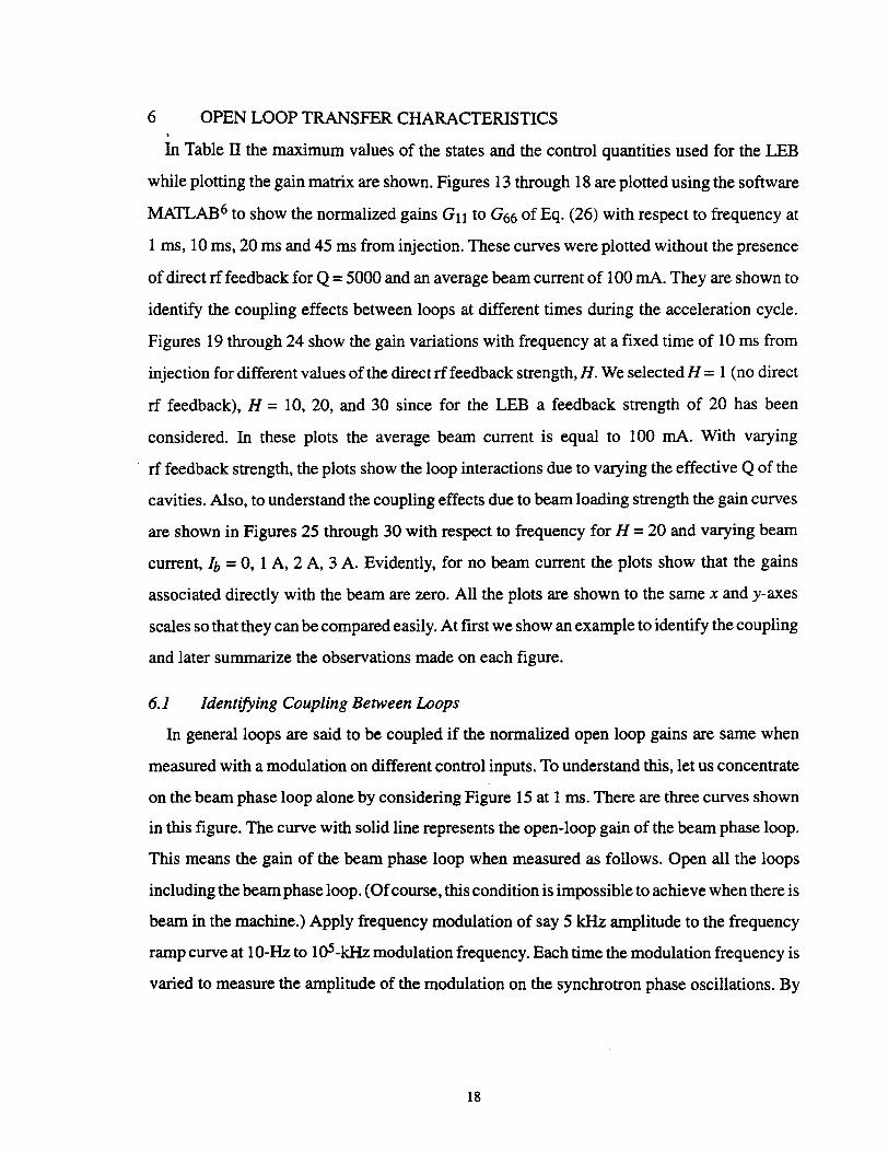
6 OPEN LOOP TRANSFER CHARACTERISTICS

In Table IT the maximum values of the states and the control quantities used for the LEB

while plotting the gain matrix are shown. Figures 13 through 18 are plotted using the software

MATLAB6 to show the normalized gains Gll to G66 of Eq. (26) with respect to frequency at

1 ms, 10 ms, 20 ms and 45 ms from injection. These curves were plotted without the presence

of direct rf feedback for Q = 5000 and an average beam current of 100 mAo They are shown to

identify the coupling effects between loops at different times during the acceleration cycle.

Figures 19 through 24 show the gain variations with frequency at a fixed time of 10 ms from

injection for different values of the direct rffeedback strength, H. We selected H = 1 (no direct

rf feedback), H = 10, 20, and 30 since for the LEB a feedback strength of 20 has been

considered. In these plots the average beam current is equal to 100 mAo With varying

rf feedback strength, the plots show the loop interactions due to varying the effective Q of the

cavities. Also, to understand the coupling effects due to beam loading strength the gain curves

are shown in Figures 25 through 30 with respect to frequency for H = 20 and varying beam

current, Ib = 0, 1 A, 2 A, 3 A. Evidently, for no beam current the plots show that the gains

associated directly with the beam are zero. All the plots are shown to the same x and y-axes

scales so that they can be compared easily. At first we show an example to identify the coupling

and later summarize the observations made on each figure.

6.1 Identifying Coupling Between Loops

In general loops are said to be coupled if the normalized open loop gains are same when

measured with a modulation on different control inputs. To understand this, let us concentrate

on the beam phase loop alone by considering Figure 15 at 1 ms. There are three curves shown

in this figure. The curve with solid line represents the open-loop gain of the beam phase loop.

This means the gain of the beam phase loop when measured as follows. Open all the loops

including the beam phase loop. (Of course, this condition is impossible to achieve when there is

beam in the machine.) Apply frequency modulation of say 5 kHz amplitude to the frequency

ramp curve at 10-Hz to lOS-kHz modulation frequency. Each time the modulation frequency is

varied to measure the amplitude of the modulation on the synchrotron phase oscillations. By

18

taking the ratio of the phase oscillation amplitude and the amplitude of the modulating ,

frequency and then normalizing by using the values shown in Table II a gain curve (G33) shown

by solid line can be obtained . As was anticipated, the curve has a peak at the synchrotron

frequency. Since the beam phase can also be affected by the amplitude and phase control on the

generator current (MC and OcpC) we need to plot the open loop gain curves for such cross

coupling. This can be done by opening all the loops and making a measurement on the beam

phase by applying a sine wave modulation on the amplitude and phase controls independently

between 10Hz to 105 kHz. The dashed line represents the open loop gain response (G34)

between the beam phase and the amplitude of the generator current. Similarly, the dash-dotted

line represents the open loop gain response (G35) between the beam phase and the phase of the

generator current.

The gain curve, G35, in Figure 15 at 1 ms is following the same amplitude as the gain curve,

G33, after 700 Hz up to 100 kHz with a peak at the synchrotron frequency. This means,

between 700 Hz and 100 kHz, the control from the beam phase loop is coupled to the local

phase loop. To make the beam phase loop operate independently of the local phase loop, they

have to be decoupled at the operating region of the beam phase loop; otherwise, they may

interact one another and ultimately cause unknown instabilities in the beam. Similarly the gain

curve, G34, intersects with the gain curve, G33, at approximately 10 kHz, meaning all three

loops are strongly coupled. Also, the figure (Figure 15 at 1 ms) shows the generator current

amplitude control has a stronger effect on the amplitude of the beam phase oscillations at

frequencies below 10kHz when compared to the amplitude of the frequency control in the

beam phase loop. Later in this section we show that a reduction in the Q of the cavity reduces

the coupling between the local amplitude loop and the beam phase loop. Whereas, the local

phase loop remains coupled to the beam phase loop even after reducing the cavity Q.

Figures 13 through 30 show that all the loops are coupled at the synchrotron frequency. At

frequencies below the synchrotron frequency we can identify coupling by taking a closer look

at individual gain plots. We present a brief summary of this below.

19

Figures 13 and 14: Synchronization and radial loops are not coupled to local amplitude and . phase loop controls below synchrotron frequencies. However, the synchronization loop has a

dominant effect on the radial position. Hence, to control the radial position when the

synchronization loop is closed from the time of injection in the LEB, a 'dead zone'

(programmable gain with radial position) may be needed in the radial loop controller. With the

dead zone, the radius can be allowed to move freely up to few millimeters around the central

orbit for synchronization. Figure 13 at 45 ms suggests an open-loop bandwidth of about

200 Hz which corresponds to a time constant of 5 ms. Therefore, ifthe synchronization loop is

closed at 45 ms, we have to achieve synchronization in less than 5 ms which demands a high

gain in this loop and consequently only a low or no gain in the radial loop could eliminate the

loop interactions.

Figures 13 and 15: The beam phase loop is coupled to the local phase loop in its operating

region. Also, by comparing the solid lines in Figures 13 and 15 at 45 ms we see that the

open-loop gain of the beam phase loop matches with that of the synchronization loop at 60 Hz.

From 60 Hz to 200 Hz the beam phase loop gain increases steeply and that of the

synchronization loop decreases to below unity. It means the coupling between the

synchronization loop and the beam phase loop is strong in this frequency band. If the

synchronization loop is arranged to operate after 45 ms, since it inevitably requires a

bandwidth of greater than 200 Hz to reach synchronism within 5 ms thereafter, the loop will

interact with the beam phase loop. Hence, by including a low-pass filter with a cutoff below

100Hz in the synchronization loop and by closing the loop much earlier than 45 ms,

interactions with beam phase loop can be greatly reduced. Alternatively, if the specifications

on the maximum synchrotron phase oscillations are relaxed to 6 degrees instead of3 degrees as

in Table II, the time required for synchronization can be reduced.

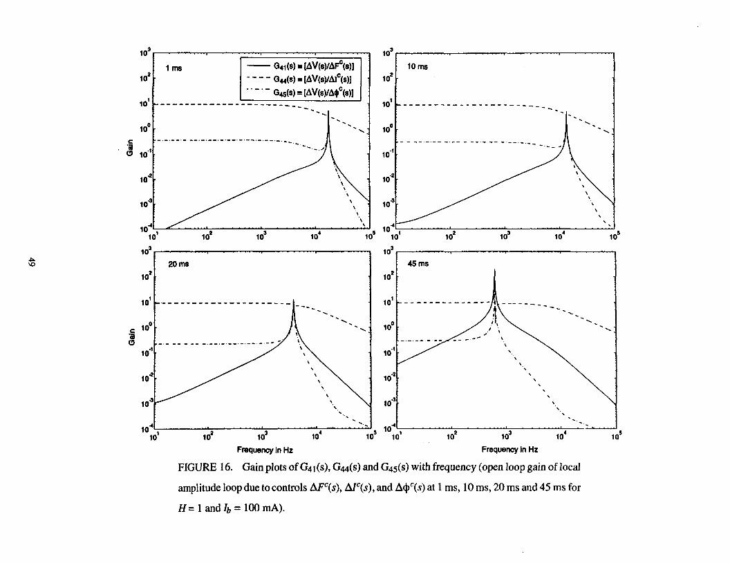
Figure 16: The global frequency control and the local phase loop control do not affect the

local amplitude loop except around synchrotron frequencies. The local amplitude loop has an

open loop bandwidth close to 100kHz.

20

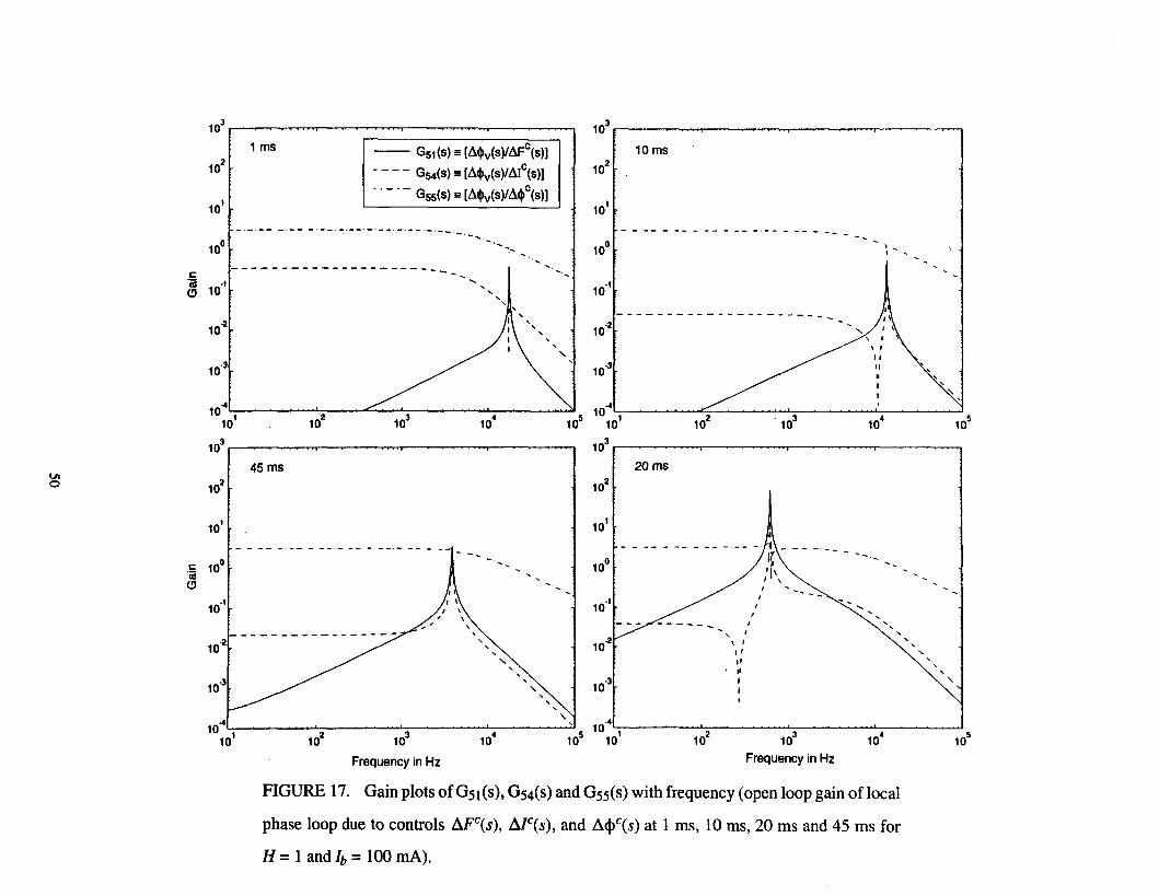
Figure 17: The global frequency control and the local amplitude loop control do not affect

the local phase loop except at synchrotron frequencies. The local phase loop has an open loop

bandwidth close to 100kHz.

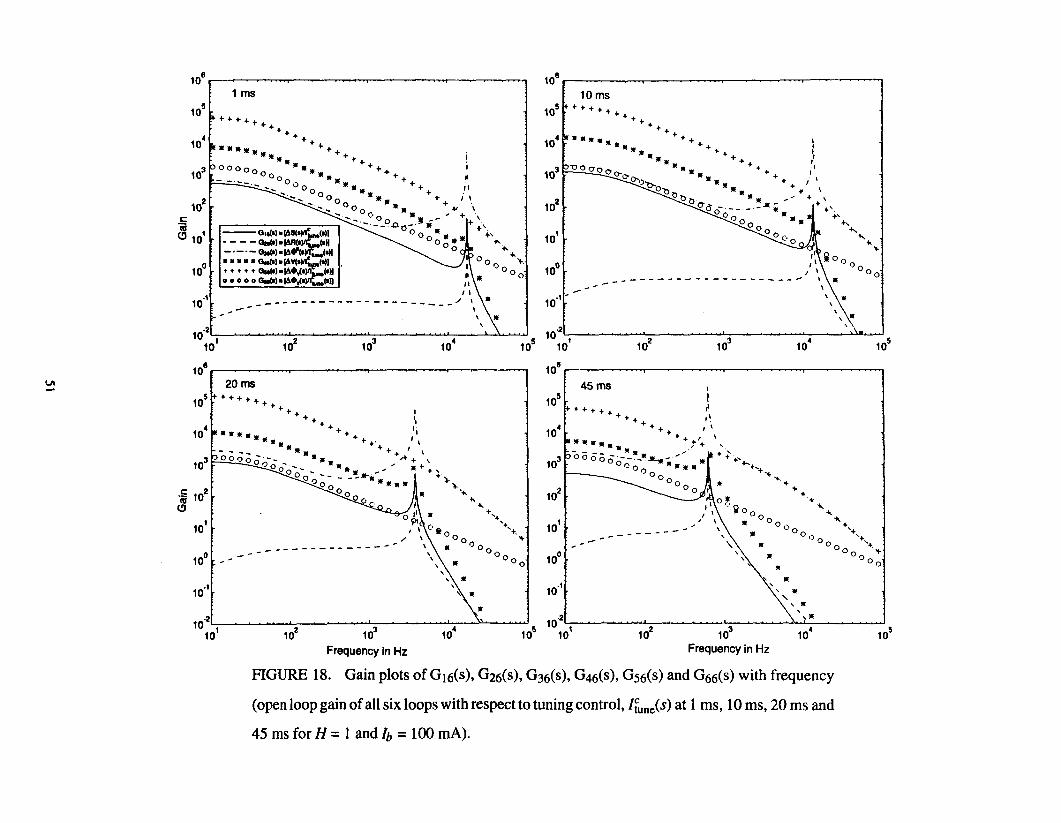
Figure 18 and 24: The tuning control, I~me' is affecting all the states including the

synchronization phase. These figures show that the cavity tuning system has to be good for the

LEB to work since all the loops are coupled to the tuning control.

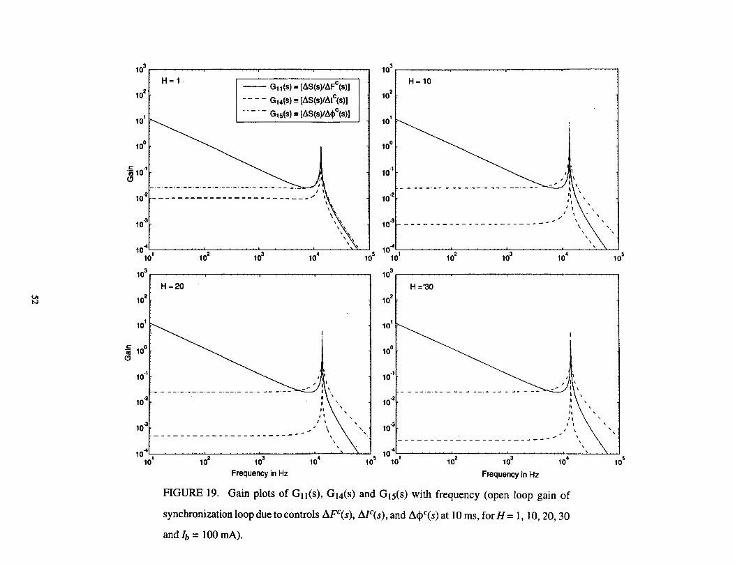
Figure 19: With the increase in the direct rf feedback, H > 1, the gain of the synchronization

loop with respect to generator current amplitude control is reduced.

Figure 20: With the increase in the direct rf feedback, H> 1, the gain of the radial loop with

respect to generator current amplitude control is reduced.

Figure 21: The beam phase loop is decoupled with the generator current amplitude control

for H = 10, 20 and 30 in its operating region around the synchrotron frequency. However, the

beam phase loop is not decoupled from the local phase loop control. One of the ways to

decouple them is by introducing a tracking band-stop filter in the local phase loop or operate it

at frequencies above the synchrotron frequency.

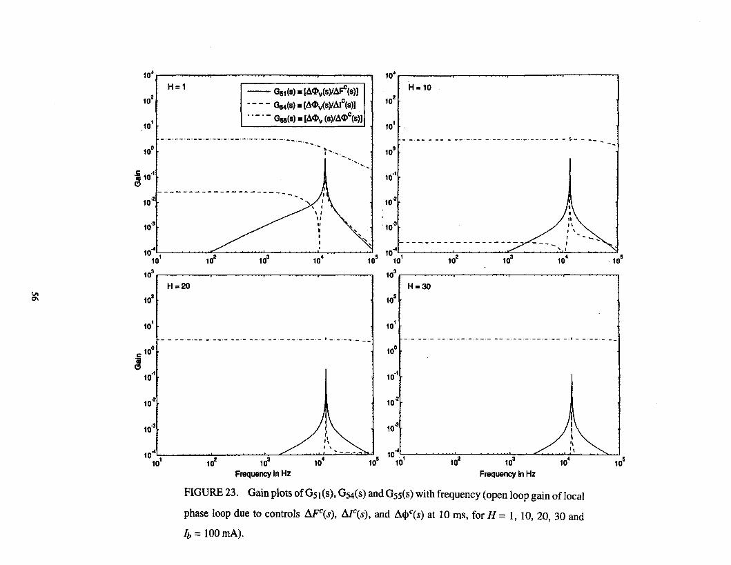
Figure 22 and 23: No significant change in the local amplitude and phase loops in the

presence of direct rf feedback.

Figures 25, 26 and 27: Increase in beam current is not significantly affecting the coupling of

the global loops with the local amplitude and phase loops.

Figure 28: The local amplitude loop is coupled strongly to the local phase loop control with

increase in beam loading.

Figure 29: The local amplitude control is coupled strongly to the local phase loop with

increase in beam loading.

21

7 CONCLUSIONS

A scientific study of the low-level rf feedback loops with rf cavity and beam dynamics for

the SSC Low Energy Booster showed clearly the interaction between all the loops. We see that

the fast and slow feedback loops are coupled at synchrotron frequencies. The synchronization

and radial loops are also coupled to one another but do not interact with the local amplitude and

phase control loops below synchrotron frequencies. Whereas the beam phase loop and the local

phase loop are coupled during the complete operating region of the beam phase loop. The

interactions between them are stronger even with a reduced Q of the cavity. One way to

decouple them is by operating the local phase loop above synchrotron frequencies or have a

tracking band-stop filter in the local phase loop. With a high Q cavity and increased beam

current the analysis showed that the local amplitude loop also has increased coupling to the

beam phase loop. Furthermore, the cavity tuning system interacts strongly with all the loops.

Hence, the tuning system must be good for other machine parameters to be under control.

The normalized open-loop gain plots drawn with respect to frequency for different control

inputs are useful to know the available bandwidth on each loop and then design appropriate

filter corner frequencies to decouple them. The method used in this paper is especially more

useful for fast-cycling synchrotrons. The decoupling can also be done by following some ofthe

techniques outlined in Reference 7 using the time varying state-space model derived in this

paper. Intuitively, the multivariable state-space control method should give better results since

all the loops are considered together while designing decoupling compensators. The results of

the systematic study on the decouplers will be reported in future.

ACKNOWLEDGEMENTS

The authors would like to thank Bob Webber for his continued encouragement to carry on

the work discussed in this paper. Also, the assistance given by G. Rees, Tai-Sen Wang and

N.K. Mahale in various technical discussions while developing the control model is gratefully

acknowledged.

22

REFERENCES . 1. F. Pedersen, "Beam Loading Effects in the CERN PS Booster," IEEE Transactions on

Nuclear Science, Vol. NS·22, No.3, June 1975.

2. Tai-Sen F. Wang, "Bunched-Beam Longitudinal Mode-Coupling and Robinson-Type

Instabilities," Particle Accelerator, Vol. 34, PP. 105-126, 1990.

3. S.R. Koscielniak and Tai-Sen F. Wang, "Compensation ofRF Transients During Injection

into the Collector Ring ofthe TRIUMF KAON Factory," Particle Accelerator Conference,

San-Francisco, May 6-9, 1991.

4. L.K Mestha, C.M. Kwan, and KS. Yeung, "Instabilities in Beam Control Feedback

Loops in Proton Synchrotrons," Accepted for publication in the Journal of Particle

Accelerators.

5. C.M. Kwan and L.K Mestha, "Simulation of Longitudinal Beam Dynamics With the

Inclusion ofRF Cavity," SSCL-617, March 1993.

6. MATLAB Reference Guide, The Math Works Inc., Natick, Mass. 01760, USA, August

1992.

7. J.M. Maciejowski, Multivariable Feedback Design, Addison-Wesley Publishing

Company, 1989.

APPENDIX A

A.i Condition for Time-Varying Approach

Solution of the second-order differential equation of the cavity for an appropriate generator

current will result into the gap voltage. For machines such as the LEB, the generator current is

driven by a variable frequency oscillator. For it to work, the gap voltage, v, must track the

voltage applied on the anode of the power amplifier. It is usual practice in the accelerator field

to represent the gap voltage and generator current as follows

23

VJwt v = e

(AI)

V· 00 By substituting I g = u;ut, a = 20., holding cavities on tune (00 R = (0) and sweeping the

frequency 00 between 'be x 47 MHz to 'be x 59.9 MHz, we must in principle obtain the gap

voltage v shown by Eq. (AI). Our simulation studies showed that the voltage was unable to

track Vinput as shown by curve with dashed line in Figure A.I. On the other hand if the generator

current was represented as

(A2)

there was good tracking as shown by curve with solid lines in Figure A.I. Small oscillations on

the curve with solid lines are due to the synchrotron frequency. With a reduced rate of change of

the accelerating frequency, 00, the tracking of the voltage was improved. This means the

modeling approach shown in Eq. (AI) is incorrect for machines like the LEB. Since the LEB

frequency is time varying we need to have a condition to know when exactly we can cross the

boundaries between time varying and time invariant approaches. Some simple equations are

derived below for the cavity parameter and accelerating frequency.

Substituting equations for v, v and v into Eq. (2), we obtain

(A3)

The right-hand side of Eq. (A3) can be written as,

(A4)

Since Vand U can be represented as phasors, we can write them as real and imaginary parts as

follows:

24

V= VR+jVI

U == UR + jUI (AS)

By substituting Eqs. (A4) and (AS) into (A3) and comparing the real and imaginary parts, the

following equation can be obtained in state space form

VR VR 0 0 0 1 0 00 00

VI 0 0 0 1 VI 00 00 0 +

VR a31 a32 a33 a34 VR 00 1 0 UR (A6)

VI a41 a42 a43 a44 VI 00 o 1 UI

where

2 ( . ) 2 a31 = -WR

+ W + wt a33 = -20 a43 = -a34

a32

- (2w+wt) +20(w+wt) a34 , ... 2(w+wt)

Equation (A6) is in the standard form

(A7)

If we assume that we have frozen the time then, det(sl - d.) = 0 is the characteristic equation.

It turns out that the characteristic equation is 4th order.

(A8)

25

where the coefficients of Eq. (A8) are given by

a2 - 4<1 + 4 (00 + oot)2 + 2 {wi - (00 + oot)2}

a1 = 40 (00 + oot)2 + 2 (00 + eM) (200 + rot) +

40 { wi - (00 + wt) 2} + 2 (00 + wt) {2w + wt + 20 (00 + wt) } 2 2

ao = [{ooi- (00+wt)2} + {2w+wt+20(00+wt)} ] . (A9)

When til = 0, the coefficients are independent of time. For simplicity we can assume that the

cavities are on tune, i.e., (O~ = (02. Now by comparing the coefficients ofEq. (A9) with those

for til = 0 we can obtain the following inequalities.

oot -« 1 00

o 1 wt 00 -»--+-00 2 002 002

o oot -»-00 00

(AW)

(A11)

(AI2)

If the inequalities presented above are satisfied, then the mathematical formulation shown in

Eq. (A I) is close to being a time invariant system. Hence, the loop models constructed based on

such an approach are accurate, even for fast-cycling machines. However, for the design

parameters of the LEB, inequality in Eq. (AI2) is violated. Hence the representation shown

by Eq. (AI) does not give accurate model. We, therefore, have to consider a more general

method as in Eq. (A2).

26

APPENDIXB

B.l Validity of Linear Model with Pedersen Model

The linear model shown in state space form of Table I can be compared to Pedersen's model}

by disabling the direct rf feedback (H = 1), the frequency control (OW C = 0), and allowing no

time variation to the cavity and beam parameters. Using the linearized version ofEq. (15) and

the tuning angle Eq. (21) and steady state Eq. (22) we get

. 0 oav - wb<j>v + owtan (<j>z) av =

~w { (I gcos<j>L - I bsin<j>S) b<j>v - I gcos<j>L b<j>c - I bsin<j>sb<j>s - sin<j>L bf}, (B 1) o

wav + 20b~v + 20wav -

~w { (Igsin<j>L - ibcos<j>S) b<j>v - Igsin<j>L b<j>c - Ibcos<j>sb<j>s - cos<j>L bf} , (B2) o

where av = OJ'.

While deriving the above equation we have assumed Kg = 1. Now by taking Laplace

Transform of Eqs. (B1) and (B2) and by assuming the Laplace parameter s ~ wtan(z} as in

Reference 1, we obtain

[

02 (tan<j>~ sin<j>s + cos<j>S) - OSCOS<j>S]

- -y 2 2 2 0

S + 20s + 0 (1 + tan <j> ) z

27

- a2y (tan<j>~sin<j>s + cos<j>S) + as (tan<j>~ - Ycos<j>S)

i + 2as + 0 2 (1 + tan \~)

iftan<j>~ (tan<j>~ - Ycos<j>S) + a (s + a) (1 + Ysin<j>S)

2 2 2 0 S + 2as + a (1 + tan <j> z )

(B3)

The sign of the transfer function connected with beam in Eq. (B3) is different since the

convention of o<t>s used in Eq. (B3) is arbitrary.

To derive the coupled transfer function with the tuning system, we rewrite Eq. (21) as

(B4)

where x = booR' a shift in resonant frequency.

Using Eq. (B4) and Eq. (22) in the linearized version ofEq. (15), and by ignoring the terms

associated with o<t>c and o<t>s we get

aav - oo()~v + aootan</>~av - aoo()</>v - oor

. 0 wav + o6cpv + owav - -owtancpz6CPv.

CB5)

Taking Laplace Transform of Eq. CB5) and assuming s ~ 00 tan{ <t>z) the following transfer

function models are derived

28

-atan<j>~ 2 2 2 0

S + 2as + a (1 + tan <j> z)

(B6) bel> (s)

v s + a

Xes) 2 2 2 0 S + 2as + a (1 + tan <j> z)

This shows our state space model meets the Robinson stability criteria for a time invariant case.

29

TABLE I: A linear state-space control model.

Xl au a l2 0 0 0 0 Xl

X2 0 a 22 a 23 a 24 a 23 0 X2

X3 0 - a 32 a 33 a 34 a 3S a 36 X3

X4 0 a 42 a 43 a 44 a 4S a 46 X4

Xs 0 a S2 a S3 a S4 ass a S6 Xs

X6 0 0 0 0 0 a 66 X6

00 0 0 0 0 ro dubB

00 0 0 0 0 0 d 2lbB

00 b33 b34 b3S 0 .S

U3 - + d31 bB + +

00 b43 b44 b4S 0 U4 C4 + d 4l bB

00 bS3 bS4 bss 0 Us Cs + dSlbB

00 0 0 0 b66 U6 C6

30

TABLE I: A linear state-space control model. (Continued)

Xl ... 6S

X2 .. 6R

X3 .. 6cpS

X4 .. 6V

.s/ S all "'"' v v

X5 .. 6cpv o

X6 .. CPz - cP z ... 6cpz

U1 - U2 - U3 - 60/ u

4 .. 6f

u5 = 6cpc

u6 ... i~une ( "'"' -KJiX6 when the loop is closed)

2 2nfrly T - S

a32 - RS

[1- oRKlb {-F21 cosCP +F22sincpS}]

a33 ... oRKlb W [F 21 sin cps + F 22 COS cpS]

o a34 - ow [F 21 tancp z + F 22H]

a35 - -oRKgw [F 21 (/gCOSCPL - jbsinCPS + igsinCPL) + F 22 (/gsinCPL - jbCOScps - igCOSCPL) ]

2 0 a36 ... F21 0wVsec cP z

o . b33 .. 1 + F21 (oVtancp z + oRKlgsinCPL) - F22 (oRKlgcosCPL - V - oVH)

b34 .. oRKlg(F21sinCPL-F22cosCPL)

b35 - oRKg {F21 (/gwcosCPL + igsinCPL) -F22 (igcosCPL - IgwsinCPL)}

31

a44 .. -000 [F u tancpOz + F 12H]

a45 = oRKg {Ig 00 (Fu cos<PL + F 12 sinCPL) - Ib (Fu sincps + F 12cosCPS) +

(F ui gsinCPL - F 12igcoscpL) }

2 ° a46 .. -F u 0(0 Vsec cP z

b44 = oRKiJ) [ - F u sin<PL + F 12cos<PL]

b45 - -oRKg[Igw(FllcosCPL +F12sin<PL) +ig(FusinCPL +F12 cos<PL)]

ass - -a35

aS6 ... -a36

bS3 - 1- b33

b54 - -b34

bS5 - -b35

a66 - -a

C4 " -Fuo(HV+wVtancpOz) -F1200(V+oHV) + FuoRKgoo (ibCOSCPs-Igsin<PL)

+ F120RKgw (- Ibsincps + IgcosCPL) + oRK/g (F 11 cosCPL + F 12sinCPL)

Cs = -F210(HV+wVtancp~) -F22w(V+oHV) +F210RKgw(Ibcos<Ps-IgsinCPL)

+ F220RKgw (- Ibsincps + IgcosCPL) + oRK!g (F21 cosCPL + F22sinCPL)

32

o .0 C6 ... - (a<j> z + <j> z)

F 11 = (oHV + oRKi bsin<j>S) I D

F 12 ... (wV + oRKibCOS<j>S) ID

33

F21 = -wiD

F22 ... oHID

TABLE II: Parameters used for normalization.

Xl = 5 m .xi = 0.01 m

x3 = 3° = 0.0524 rad xT = 8000 volts

x'5 = 3° = 0.0524 rad x'6 = 3° = 0.0524 rad

u'i = 5000 Hz = ui = u3 x~ = 5.7 X 10-4 Amp

Xs = 0.1576 rad

x'6 = 100 Amp

Kg = 700

R = 182 kQ

Q = 5000

<PL = 0

lb = 100 rnA

34

DDS-Direct Digital Synthesizer TDC-Time-to-Digital Converter PD-Phase Detector PS-Phase Shifter PA-Power Amplifier TBR-Tuning Bias Regulator

GLOBAL AMPLITUDE HARDWARE

FIGURE 1. RF beam control loops planned for the SSC Low Energy Booster.

35

R

FIGURE 2. Equivalent circuit of the Cavity.

36

Synchronization Loop

i f>S

Radial Loop

i f>R

Bias L.-_~ Regulator

t

v

FIGURE 3. Schematic loop diagram of Figure 1 showing control and measured quantities.

v

~--;===tJ"----J_--'-----. V ideal

FIGURE 4. Phasor diagram showing the relations between generator current, ig , beam

current, ib, and the gap voltage, v at a given time.

37

a s+a

FIGURE 5. Cavity tuning loop (without feedforward control).

38

Tracking code output Non-linear model output

e ~ 0.5 .5 r:::

I/)

! Q) E .5

~ 0 .(i;

8.

r::: 0 E I/) 0

~ -0.5 Q. a; -0 =0

a: as a:

-1~------------~------------~----~ o 0.02 0.04 0.02 0.04

Time in seconds Time in seconds

FIGURE 6. Variation of mean radial orbit with time for 10 Me V injection energy error

predicted using tracking code and the non-linear model.

39

-4 (a) 1 r-x_1_0_---'_--.-____ --.

-4 (b) 1 X 10

", \ 0.5 I

n,. " 'I ~ ,\ {I, ,

I I I , ,

I I e 0.5 ~ CD

~ 0[\ , I , I , I

, I , , I I

o I , , I , I , , ,

I , , , , ! -0) ~ -0.5 i II: " V I

-1L-------------------~ o 0.5 1 -1

4.7

(c) X 10-5

(/)

! CD E

5

0 I

d , I ,

I

p , \ , \ , I , I I I I

.5 c: .2 :t= (/)

I I I I I I , I ,

8. a; i -5 II:

, '

0.02

I , I , \ , \

0.021 Time in seconds

X 10-3 (d) X 10-5

5

, \ , \

I I \ ,

I I \ I

0.022

0

-5

0.04 -- Tracking code - - - - Non-linear model

I , , I , I I

I , I I , I I I , I I , I , , , , ,

V\' I

V\l V" V\

4.8

0.045 Time in seconds

(I, ,\ 1\

I I

, I , , I

, , I

, , , , , , , ,

VJ

4.9

X 10-3

0.05

FIGURE 7. Variation of mean radial orbit shift with time (expanded scale of Figure 6).

40

Tracking code output (8) 40..------.--------..---, (b Non-linear model output

>40~---------------~------------~~

I en Q)

"0

.5 Q)

1Q oJ: a.

-40~------~------~--~

o 0.02 0.04 Time in seconds

~ ! en Q) "0

.5 Q) UJ t'CI

oJ: a.

0.02 0.04 Time in seconds

FIGURE 8. Variation of particle phase with time for 10 Me V injection energy error

predicted using tracking code and the non-linear model.

41

(J) CD ! CI CD '0

.5 CD (J) as or; Q.

50.---------~--------~

o

I V

:~ -50~------------------~ o 0.5 1

X 10-3

o

-20

\

, ' , '

4.7

J

, , , , ,

, , I

I " , I I

J J

4.8 4.9

X 10-3

10~--------~------~

10 , , I I I I , I I

, ,. , ,

I ,

I \ I ,

I \ 0, \ I

I ,

I \ I I , I \ I ' , \ I , I \ \ \

-10

0.02 0.021 0.022 -w'04 0.045 0.05 Time in seconds

-- Tracking code Time in seconds

- - - - Non-linear model

FIGURE 9. Variation of particle phase with time (expanded scale of Figure 8).

42

Jg g .5 -CD CI

~ g CD 0 c: I!? .! I!?

CD

~ -(5 > a. as S2.

Tracking code output en X 10

4 Non-linear model output == 0 > .5 -0 CD CI as

~ CD 0 c:

-1 -1 I!? CD -I!?

CD -2 -2 CI

S 0 > a.

0 0.02 0.04 0 0.02 0.04 as CJ -Time in seconds Time in seconds

FIGURE 10. Variation of voltage error (gap voltage-reference voltage) with time predicted

using tracking code and the non-linear model.

43

-CD C> S g CD o c: ~

i CD C>

~ g c. eo

C!) - o

2000

1000

0

! -1000 C>

, , I , , ,

\

~ g ~ -2008,02

\ , , I ,

\ I I

I ,

0.5

,\ I I

\ \.

0.021

\ ,

Time in seconds

, I

\.

\ I I

1 X 10-3

0.022

o~~------~----~--~

-1000 , , -2000 '

-3000

-4000

, I , , , '

" I

J

, I , , , , I

I

-5000L------------~ 4.7 4.8 4.9

X 10-3

3OO0~------~--------~

2000

1000

-1000

0.045 0.05

-- Tracking code Time in seconds

- - - - Non-linear model

FIGURE 11. Variation of cavity gap voltage error with time (expanded scale of Figure 10).

44

U)

~ 60, C) _

~ II

.E 40 II e 11

~ 11

2~~------~----~-.

1

o ---'------.....---"--Q) 11 ~ 20,1 Q. 1

-1 \

o ~------------

o 0.5 1

X 10-3

_3L-~------~----~~

4.7 4.8 4.9

X 10-3 U)

m 2~--------~---------. 2~--------~-------. C) Q) "0

.E e e ... Q)

Q)

1

U)

1! -1 Q.

1

0.021 0.022 ~04 0.045 0.05 Time in seconds Time in seconds

-- Tracking code - - - - Non-linear model

FIGURE 12. Variation of cavity gap phase error with time (expanded scale).

45

1 ms -- Gll(S) = [~S(s)/~FC(S)] - - - - G14(S) = [~S(s)/~IC(S)J

10' .. - . - G15(S) = [~S(s)/~cj)C(s)]

-------------------------

10 ms

10'

I

" 10-2 --~----~~--~~--~~--~~--~~---_~-_-_~_/' '.

10-3

\

, , , ., "

10~~~--~~~------~----~~~~~~~ 10~L-~--~~--~~~~~~--~--~~'~~ 10' 10

2 10

3 10· 10! 101 102 103 10· 105

103 103 .-----~~.........---~~~..-~--~-.......,.--~~~...,

20ms 45ms

, , 10~L---~~~--~----~----~~--~~~~ 10~L---~~~~--~~~~----~~~~~~

101 102 103 10· 105 10' 102 103 10· 105

Frequency in Hz Frequency in Hz

FIGURE 13. Gain plots of Gll(S), GI4(S) and GI5(S) with frequency (open loop gain of

synchronization loop due to controls MC(s), MC(s), and ~<t>C(s) at 1 ms, 10 ms, 20 ms and

45 ms for H = 1 and Ib = 100 rnA).

103

102

10t

c: 10° 'iii C!)

10,t

10'2

10'3

... 10 t

10

103

-'" ....:I

102

lOt

c: 10° "iii

C!)

10,t

10'2

10'3

10'" 10

1

103

1 ms -- G22(S) 55 [~R(s)/~FC(s)) 10

2 10 ms

- - - - G24(S) 55 [~R(S)/~lc(s)] ' , - ,- G2S(S) 55 [~R(s)/~cjIc(s)l 10t

10°

10't

10'2

\~ '\ ' I

'I I I

10-3 ... '" ~ \ !I. .... '\. , ~ \ " , .... I \ . '" \ ,. ... " \ ~r\. " ,

..." /,'" \ ... ,. ",,,,/ '\ .:\.

... .... ... ...

10'" .... . .-- ..-f'" .... ... "

102

103

104

105 lOt 102

103

104

103

20ms 10

2 45ms

10t

100

10'1

10'2 ~ \

~ \' ~ ~ ,

/~ , ,

,~ ... ~ "" " , , ~~

10,3 ,~,,: ... , , ",,-:,/ ~ , , ... -;.~ .... ,

, , ,/ ,

" /, ,., 10-4 : -;. , :...'~ ,/ ,.,

102

103

104

105

101

102

103

104


FIGURE 14. Gain plots of G22( s), G24( s) and G2S( s) with frequency (open loop gain of radial

loop due to controls Il.FC(s), MC(s), and Il.<j>C(s) at 1 ms, 10 ms, 20 ms and 45 ms for H = 1 and

Ib = lOOmA).

105

105

1 ms -- G33(S) 5! [L\cIIS(S)/L\F

c(S))

- - - - G34(S) E [L\cIIS(s)/L\)c(S))

.. - . - G3S(s) E [L\cIIS(s)/L\cIIc(s))

10° ______________________ _

20ms

-------------------

I" ~ ,. ,

\

\

\

, ,

, , \

10 ms

10° - - - - - - - - - - - - - - - - - - - - - - - - -

- --'- -- -

, ,

, , \

"

10 ... L~~~ ......... _:__-~~"'"'"'_:::_--~"'"""7~~~-....J 10·4L-~-~ .......... _:__~~~"'"'"'_:::_---"""'_:_--~-....J 10' 102 103 10· 105 10' 10

2 10

3 10· 105


FIGURE 15. Gain plots ofG33(S), G34(S) and G3S(S) with frequency (open loop gain ofbearn

phase loop due to controls M'C(s) , MC(s), and ~C(s) at 1 rns, 10 rns, 20 rns and 45 rns for

H = 1 and Ib = 100 rnA).

103r-~~~~~~~==~======~======~ -- G41(S). [.1 V(s)/.1~(s)] 1 ms - - - - G .... (S). [.1V(s)/.1IC(s)]

"" -" - G45(S) II [.1V(s)/.1+C(s)]

10' -------------------- __

c -.-.-_.-._-.-.--.-.--.-. __ .-._-.- -"ii CJ 10"'

10-4~~~~~--~~--~--~~~--~~~ 10'

10'r---~~~--~~~~--~~~~~~~

20ms

10' .- - - - - - - - - - - - - - - - - - - - -

10° c 'ii CJ _.-. __ .- -- -. __ ._. __ ._._-_.--

10"'

10"

- --

, ,

\

'.

105 10-4~------~----~--~--~~~~----~ 1~ 1~ 1~ 10·

Frequency In Hz

10ms

10' - - - - - - - - - - - - - - - - - - - - __

- - -- - -- - -- - -- - -- - -- - -

--

\ , ,

10-4L---~--~~ ______ ~ __ ~ __ ~~~~~~ 10' 102 10' 10· 105

1~.---~~-r--~~~~----~~--~~~~

45ms

10"2 , , ,

10-3 ,

\ ,

10-4 10' 10

2 103 10· 105

Frequency In Hz

FIGURE 16. Gain plots ofG41(S), G44(S) and G45(S) with frequency (open loop gain oflocal

amplitude loop due to controls M'C(s), MC(s) , and L\C(s) at 1 ms, 10 ms, 20 ms and 45 ms for

H= 1 and1b = 100 rnA).

VI o

1 ms -- GS1(s) = [L1~(s)/L1Fc(S)] - - - - G54(S) E [L1c1lv(s)/L1IC(s))

.. - . - GSS(S) E [ L1c1lv(s)/L1c1lC(s»)

- .-. -- ._. - -.- --. -.--. _.- -. - .-- ._._-.........

--------------------- '. --" " " " " " " "

" "

10·4L-~_~_""'_:__--...c;;~_'_:~~~-......,...~-~ .......... 10' 10

2 10

3 10

4 10

5

103~~~~~--~~~~--~~~~~~~~

45ms

10'

" " " " " " "

" 10·4L-~-~ ........ _=__---......1..;:__-~~"'""7~-~--....... 10' 10

2 10

3 10

4 10

5

Frequency in Hz

10ms

- - -- - -- - -- - -- -.-- - -- - --

---------------------

10.3

10-4 10

1 10

2 . 103

103

102

10.3

20ms

I

- - -- - -- - -- - -- - , - - - _._-I{

" , , " II

" , , ,

I

I

It, , I ,

'- -

10-4 10' 10

3

Frequency in Hz

1 , , ,

, ,I

" " , , , , " "

" " " "


phase loop due to controls M'C(s), MC(s), and d<j>C(s) at 1 ms, 10 ms, 20 ms and 45 ms for

H = 1 and Ib = 100 rnA).

"

VI -

1 ms

"

10·' ------------------

10.2

101

108

20ms

----------- ---

10 ms +++++++

++++ ++

++ +-1-

-1-+ ++

+ + + +

+ -I ..

--------------------

\ " .. ., , I'

\

+ \ + ,

+. +,

\

+,. +~

\ .

< ...

10·2L:-~~-~........,~~~~.......J7_-~~~~-~~......,......J 105 10' 10

2 10

3 10

4 10

5

108r-______ ~~--------~~--~~--~~------~_,

45ms

101

---- • • • •

• • ,

" • , . ,

10·2L __ ~~~'"'-_~~_~---'--__ ~~~..J..-:--""';"--~~.....J 10·2L-~_~~~.L-_~_~~"""'_~~~~""""_._~_~~...J

1~ 1~ 1~ 1~ 1~ 1~ 1~ 1~ 1~ 1~ Frequency in Hz Frequency in Hz

FIGURE 18. Gain plots ofG16(S), G26(S), G36(S), G46(S), G56(S) and G66(S) with frequency

(open loop gain of all six loops with respect to tuning control, I~me(s) at 1 ms, 10 ms, 20 ms and

45 ms for H = 1 and Ib = 100 rnA).

H= 1 . -- Gll(S)!!! [6S(s)/6F

c(s))

- - - - GI4(S)!!! [6S(s)/6Ic(s))

10' .. - . - G1S(S)!!! [6S(s)/6c11c(s))

.~ 10" ~ I

II I I

10~ ----------------------- __ , I

, , , "

" '1\\ 10~·L---~--~~~--~~~~~~~----~~~

10' 102 103 104

105

103r-______ ~r_--~~~~--~~~--~~~~

H=20

10'

, ,

H = 10

10'

10.4

10' 102

103

103

H='30

102

10'

100

, 10~'L-----~--~--~~~~----~~~--~'~~~ 10~'L-----~~~----~~~--------~--~~~ 1~ 1~ 1~ 1~ 1~ 1~ 1~ 1~ 1~ 1~


FIGURE 19. Gain plots of GIl(S), G14(S) and G15(S) with frequency (open loop gain of

synchronization loop due to controls IlpC(s), A/C(s), and Il<l>C(s) at 10 ms, for H = 1, 10,20,30

and Ib = 100 rnA).

H .. 1 -- G22(S). [M(S)/A~(S)]

H= 10

- - - - G24(S). [AR(s)/Alc(S»

.. - . - G25(S). [M(s)/A,c(s»)

H .. 20 H=30

FIGURE 20. Gain plots ofG22(S), G24(S) and G25(S) with frequency (open loop gain of radial

loop due to controls IlPC(s), MC(s) , and Il<j>C(s) at 10 ms, for H = 1, 10, 20, 30 and

Ib = 100 rnA).

103

103

H == 1 H = 10 10

2 -- G33(S)!! [A<l>S(s)/AFC(s)) 102

- - - - G34(S) II [A<l>S(s)/AIC(s)) , \

10' .. - . - G3S(S) II [A<l>S(s)/A<l>C(s)) 10' ,I' I ' I ,

I I

10° , " 10° ------------------------- , " \ , , ' \ C / ,

/ 'iii / , 10" ------------------ -:; ~-C) 10" , \

\ ,

\ , , 10.2 10.2 \ ,

\ \

10.3 10.3

10" 10' 10

2 10

3 10

4 10

5 10"

10' 102

103 10· 10

5

103

103

VI H=20 H=30 ~

102

102

10' 101 , \

\ \ I ,

I I I

10° , I 10° , II

c: 1\

'\ 'iii C)

10.1 ' \ 10.1 I

\ , , \

10.2 \ 10.2 , , ,

- -- - -- , , , 10-3

, , 10.3

10'· 10

1 10

2 10

3 10· 105

10" 10

1 10

2 10

3 10· 105


FIGURE 21. Gain plots ofG33(S), G34(S) and G35(S) with frequency (open loop gain of beam

phase loop due to controls ilFC(s), ilJC(s), and ilCPC(s) at 10 ms, for H = 1, 10, 20, 30 and

Ib = IDOmA).

c ·i

H=1 -- G .. 1(S). [AV(s)lA~(S)) H= 10

- - - - G .... (S). [AV(s)lttr(S)]

.. - . - G045(S). [AV(s)lAcz,C(s))

10' - - - - - - - - - - - - - - - - - - - - -_ -- .. 10'

10° - - - - - - - - - - - - - - - - - - - - - - - - - -_. _.- _._. -_._.- -._. __ . -. __ .-.- -. -. --.

_._. __ ._._- - -_._.-_.- --.-.-- -.--10-2

10" \ ,

'. .. 10" 105 10'

10~~--~--~--~----~~----~~----~ 1~ 1~ 1~ 1~ 102 103

1~~--~~~--------r-~~---~--~~~ 103

H=30

102

10'

10° ---------------------------------

I' \

104

----

(!J ., 10

.a _._-_._. __ :_. __ .- -_._._- - --.- -- -.-10 .

10-3

. , I . ,. ,

--,.

10-2 _._. __ ._. __ ._. __ ._. __ .- -_.- -- _. __ ._.-_. .-.

10"

10~~------~~~----~----~~~----~ 10 .. L-------~~--~~~----~~~----~~ 10' 102 10

3 10

4 10

5 10' 10

2 10

3 10

4 10

5

Frequency In Hz Frequency In Hz

FIGURE 22. Gain plots ofG41(S), G44(S) and G4S(S) with frequency (open loop gain oflocal

amplitude loop due to controls Il.FC(s), MC(s), and ~<t>C(s) at to ms, for H = 1, to, 20, 30 and

Ib = 100 rnA).

10'

10-2

H=1 -- GS1(S). (a~v(s)/aF'(S)J c • - - - G54(S). (a~v(s)/& (S)J

•. - . - G55(S). (a~V (s)la~C(s)J

-.-. -_._. --. _. -_.- . __ ._. __ . -. --.-. --'- -......... t· ............

----------------------

H= 10

10'

- -.--.- -- - -- - -- - --.- -- _. __ .- -- - ',.- - -- --

10~ 10' 103 10· 10

5 tO~

to' 102

103

102

10'

103

H .. 20 H=30

102

10'

- - -- _._- -.--.- -_.- -_.- -_.- -_._. __ .- . _._. __ .- -- _. _______ . __ ._. __ . ____ . __ . ___ • ____ .4 ____ . __ _

10-2

FIGURE 23. Gain plots ofG51(S), G54(S) and G55(S) with frequency (open loop gain of local

phase loop due to controls MC(s) , A/C(s), and L\<j>C(s) at 10 ms, for H = 1, 10, 20, 30 and

Ib = 100 rnA).

10-2 10

1

V. 10·

....,J

105

10·

103

C ·iii (!J

102

101

10°

10.1

10.2

101

H= 1

-----------------------

H=20

- - -'. '. ,

\ I

,~ , ---------~-----------.

1H = 10 105 + .. + + + + ••

++++ +.

104 + + + +

+ + + + il + + + I,

103 + + I,

+ * + + ' .. '

H=30

3 1II111 ••• 10 ~----.: -."

-----------------

-. •• •• ·11. I

\ I I

•• • .,. -.. -----------~---------

"

+ ~, +"+ ....

, ,

..

103

Frequency In Hz

10·2.L-.~_~~ ...... ,.__~~~~L----~~...-.-~-~~ 10

5 10

1 10

2 10

3 10

4 10

5

Frequency In Hz

FIGURE 24. Oain plots of 016(S), 026(S), 036(S), 046(S), 056(S) and 066(S) with frequency

(open loop gain of all six loops with respectto tuning control, Ifune<s) at 10 ms for H = 1, 10,20,

30 and Ib = 100 rnA).

103

102

10'

10-2

Ib= 1A -- G11(S) e [~S(s)/~P:(s)] • - - - G'4(S)!II [~S(s)/~f(s)] .. - . - G'S(S)!II [~S(s)/~.C(s)]

---------------------, \

---'" \

, '. ,

103

102

10'

10-3

Ib=2A

------------------------,

-- \ ,

'. '.

, \

10~'L-------~---------~---~----~--~~~ 10~·L-------~~--~~~~------~--~~~ 10' 102 103 10' 105 10' 102 103 10' 105

1~~--~~~~--~~~---~~ __ ~ __ ~~~

\ , -------------------------- \

'. , , ,

10~L-------~~--~~~---------~--~~~ 10' 10

2 103 10' 105

Frequency In Hz

FIGURE 25. Gain plots of Gll(S), GI4(S) and GI5(S) with frequency (open loop gain of

synchronization loop due to controls MC(s), MC(s), and d<j>C(s) at 10 ms, for H = 20 and

Ib=1,2,3A).

103

102

101

10° C °ii o

Cl 1001

1002

10-3

10" 10

1

VI \0

Ib= 1A

102

103

-- G22(S). [.1A(s)/.1Fl(s)J

- - - - G24(S) a [.1A(s)/.1IC(S»

~=2A 10

2

o 0 - 0 - G25(S). [.1A(s)/.1,C(s)J 10

1

10°

1001

j , ,'. \ 10

02

.,." II ......... ~,I !:~"" .," .\ ..... , ,

10-3

~. , , I \ 10"

101

103

Frequency in Hz

~

~

102

103

FIGURE 26. Gain plots of G22( s), G24( s) and G2S( s) with frequency (open loop gain of radial

loop due to controls MC(s), MC(s), and ~<t>C(s) at 10 ms, for H = 20 and Ib = 1,2,3 A).

, \ , I '

103

102

10'

Ib = 2A

I , \ -- G33(S). [~~S{s)/~FC{s)] • - - - G34(S). [~~S(s)/AIC{s)] .. - . - G35(S). [~~S{s)/~~C(s)] I I ' 'I ' , I-_

, , I ,

~

" " , \

\

, , , , ,

10°

10·\

10.2

, 10-3 ,

105

10'" 10'

103

Frequency in Hz

102

, , , ,

I I ~

" " 1\ , \

FIGURE 27. Gain plots of G33( s), G34( s) and G35( s) with frequency (open loop gain of beam

phase loop due to controls MC(s), MC(s), and ~C(s) at 10 ms, for H = 20 and Ib = 1,2,3 A).

, , , , , , ,

103

Ib = OA -- G41(S) E [~V(s)/~FC(s)] 10

2 - - - - G44(S) E [~V(S)/~IC(s)1

10' .. _. - G4S(S) E [~V(s)/~Cl>C(s)]

~.

10 .. .."....-~~'"'""7~--'· .... ~·.........J.-::--~~~......,...-~~.....J

10' 102

103

104

105

1~r---~~~~~~~--~~~~~--~-,

103

Ib = 1A

102

101

10° I 1\ - - - - - - - - - - - - - - - - - - - - - - - - - -.... - \ - - - - -

~ I, 10·' - - - - - - - - - - - - - - - - - - - - - - - \

10.2

10.3

10" 10'

103

102

102

103

Ib = 3A

104

III

, I \ -~ I

------------------------ - - II '-,- - - --

I

105

10·4L-_~~'"'""7_-~""""-:--~~~--'-;--~~"""" 10·4,-:-_~~~_-~ ........ -:---~~""""'---:--~_~--...J 10' 102 103 10

4 10

5 10' 10

2 10

3 10

4 10

5

Frequency in Hz Frequency in Hz I


amplitude loop due to controls MC(s), MC(s) , and L\<pC(s) at 10 ms, for H = 20 and

Ib = 0, 1,2,3 A).

-- G51(S) E [~$v(S)/~Fc(s)l - - - - G54(S) E [~$v(s)/~lc(s)l .. - . - G55(S) E [~$V (s)/~$C(S)]

- - -- - -- - -- _._- - --.-.-- - -- - -- - -- -'-- - -

10·4L--~~~"""""",,-~~~"'-:c--~~""""'-:---~'-""""" 10

1 10

2 10

3 10

4 10

5

103r---~~_r~~~~~~~~~--~~~

- - __ . ___ . ______ . ___ . ___ . ___ - __ - 1.- _____ _

" " , , , ,

, , \,

"

--- --10·4L--~~~......&..;~~~~'"7-~~""""'-;--~~~""

101

102

103

104

105

Frequency In Hz

__________________________ i ______ _

10.2

10.3

10"" 10

1 10

2 10

3

103

Ib = 3A

102

10.3 - - - - - - - - - - - - - - - - -

-

I ,

, I I

" " ,\ , '~ ,

I , I

"

104

I I I , " " , , , ~ ,

-, I

-- -

105

\1

II Y

10""L----~~-£----~~~~----~~--~~~ 10

1 103 10

4 105

Frequency in Hz

FIGURE 29. Gain plotsofGSl(S), GS4(S) and Gss(s) with frequency (open loop gain of local

phase loop due to controls MC(s), MC(s), and ~C(s) at 10 ms, for H = 20 and

Ib = 0, 1, 2, 3 A).

c: 'iii CJ

c: 'iii CJ

10"

Ib= OA +++++

+++ ++

++ ++

++

iiiiili iii.

iliila

102 ilili

101

10°

10.1

--- G,.,s) .(6S'syf~,S)) - - - - G .. ,s) • (.1R,I)II '")) - . - . - G .. ,s) .(6t(I~")) ••••• o..,s) .(6V'"~")) + + + + + Gse'") .(~'")II '"))

+ + + 0 0 0 0 0 Goo,") • (6+.'")lIt:'")J ++

++ ++

++ i-+

++ ++

+i-iI •• ++ ilii

iii iI fir liIiili

wili! !i1l1~o

•

10'"

105

10·

103

102

101

10°

10.1 '- , ,

10·2L-~~~~"""":--__ ~~~~~~~-..-.I ____ ~..J 10'2L-~~~~""""::---_~_~_~_~~,-:-~~~~"'"

101

102

103

10· 105 101

102 103 104

105

108 10er-~----~~---~~~-~~----~~-~---,

105

10·

103

102

101

10°

10.1

---------------------

••••••• •• •• •• •• •• ••

-------------- -----

I I I

" i' \

, ,

FIGURE 30. Gain plots of GI6(S), G26(S), G36(S), G46(S), G56(S) and G66(S) with frequency

(open loop gain of all six loops with respect to tuning control, Ifunis) at 10 ms for H = 20 and

Ib = 0, 1, 2, 3 A).

, ,

,!g "0

7

6

> 5 .5 Q) C) as g 4 Q. as C)

~ ~ u

--- Tracking with ig = 1geJJIddt - - - - - Tracking with ig = IgeJOlI

Time in seconds

FIGURE A. I. Cavity gap voltage tracked using the representations ig = Igeflot and

ig = Igt! f wdr for the complete acceleration cycle of the LEB.

64

interaction between beam control and rf feedback...

Documents