interacting particle systems - avcr.czstaff.utia.cas.cz/swart/skripta.pdf · 4 contents preface...
TRANSCRIPT

Interacting Particle Systems
J.M. Swart
July 20, 2011

2

Contents
1 Construction of particle systems 71.1 Probability on Polish spaces . . . . . . . . . . . . . . . . . . . . . . 71.2 Markov chains . . . . . . . . . . . . . . . . . . . . . . . . . . . . . . 101.3 Feller processes . . . . . . . . . . . . . . . . . . . . . . . . . . . . . 121.4 Poisson point processes . . . . . . . . . . . . . . . . . . . . . . . . . 161.5 Poisson construction of Markov processes . . . . . . . . . . . . . . . 201.6 Poisson construction of particle systems . . . . . . . . . . . . . . . . 241.7 Generator construction of particle systems . . . . . . . . . . . . . . 29
2 The contact process 372.1 Definition of the model . . . . . . . . . . . . . . . . . . . . . . . . . 372.2 The survival probability . . . . . . . . . . . . . . . . . . . . . . . . 432.3 Extinction . . . . . . . . . . . . . . . . . . . . . . . . . . . . . . . . 462.4 Oriented percolation . . . . . . . . . . . . . . . . . . . . . . . . . . 472.5 Survival . . . . . . . . . . . . . . . . . . . . . . . . . . . . . . . . . 502.6 K-dependence . . . . . . . . . . . . . . . . . . . . . . . . . . . . . . 532.7 The upper invariant law . . . . . . . . . . . . . . . . . . . . . . . . 562.8 Ergodic behavior . . . . . . . . . . . . . . . . . . . . . . . . . . . . 592.9 Other topics . . . . . . . . . . . . . . . . . . . . . . . . . . . . . . . 65
3 The Ising model 673.1 Introduction . . . . . . . . . . . . . . . . . . . . . . . . . . . . . . . 673.2 Definition, construction, and ergodicity . . . . . . . . . . . . . . . . 683.3 Gibbs measures and finite systems . . . . . . . . . . . . . . . . . . . 733.4 The upper and lower invariant laws . . . . . . . . . . . . . . . . . . 783.5 The spontaneous magnetization . . . . . . . . . . . . . . . . . . . . 793.6 Existence of a phase transition . . . . . . . . . . . . . . . . . . . . . 843.7 Other topics . . . . . . . . . . . . . . . . . . . . . . . . . . . . . . . 88
4 Voter models 914.1 The basic voter model . . . . . . . . . . . . . . . . . . . . . . . . . 914.2 Coalescing ancestries . . . . . . . . . . . . . . . . . . . . . . . . . . 924.3 Duality . . . . . . . . . . . . . . . . . . . . . . . . . . . . . . . . . . 934.4 Clustering versus stability . . . . . . . . . . . . . . . . . . . . . . . 964.5 Selection and mutation . . . . . . . . . . . . . . . . . . . . . . . . . 974.6 Rebellious voter models . . . . . . . . . . . . . . . . . . . . . . . . 100
3

4 CONTENTS
Preface
Interacting particle systems, in the sense we will be using the word in these lec-ture notes, are countable systems of locally interacting Markov processes. Eachinteracting particle system is define on a lattice: a countable set with (usually)some concept of distance defined on it; the canonical choice is the d-dimensionalinteger lattice Zd. On each point in this lattice, there is situated a continuous-timeMarkov process with a finite state space (often even of cardinality two) whose jumprates depend on the states of the Markov processes on near-by sites. Interactingparticle systems are often used as extremely simplified ‘toy models’ for stochasticphenomena that involve a spatial structure.
Although the definition of an interacting particle system often looks very simple,and problems of existence and uniqueness have long been settled, it is often sur-prisingly difficult to prove anything nontrivial about its behavior. With a fewexceptions, explicit calculations tend not to be feasible, so one has to be satisfiedwith qualitative statements and some explicit bounds. Despite intensive researchfor over more than thirty years, some easy-to-formulate problems still remain openwhile the solution of others has required the development of nontrivial and com-plicated techniques.
Luckily, as a reward for all this, it turns out that despite their simple rules, inter-acting particle systems are often remarkably subtle models that capture the sortof phenomena one is interested in much better than might initially be expected.Thus, while it may seem outrageous to assume that “Plants of a certain type oc-cupy points in the square lattice Z2, live for an exponential time with mean one,and place seeds on unoccupied neighboring sites with rate λ” it turns out that mak-ing the model more realistic often does not change much in its overall behavior.Indeed, there is a general philosophy in the field, that is still unsufficiently under-stood, which says that interacting particle systems come in ‘universality classes’with the property that all models in one class have roughly the same behavior.
As a mathematical discipline, the subject of interacting particle systems is stillrelatively young. It started around 1970 with the work of R.L. Dobrushin andF. Spitzer,, with many other authors joining in during the next few years. By1975, general existence and uniqueness questions had been settled, four classicmodels had been introduced (the exclusion process, the stochastic Ising model,the voter model and the contact process), and elementary (and less elementary)properties of these models had been proved. In 1985, when Liggett’s published hisfamous book [Lig85], the subject had established itself as a mature field of study.Since then, it has continued to grow rapidly, to the point where it is impossibleto accurately capture the state of the art in a single book. Indeed, it would be
CONTENTS 5
possible to write a book on each of the four classic models mentioned above, whilemany new models have been introduced and studied.While interacting particle systems, in the narrow sense indicated above, have ap-parently not been the subject of mathematical study before 1970, the subject hasclose links to some problems that are considerably older. In particular, the Isingmodel (without time evolution) has been studied since 1925 while both the Isingmodel and the contact process have close connections to percolation, which hasbeen studied since the late 1950-ies. In recent years, more links between inter-acting particle systems and other, older subjects of mathematical research havebeen established, and the field continues to recieve new impulses not only fromthe applied, but also from the more theoretical side.

6 CONTENTS

Chapter 1
Construction of interactingparticle systems
In this section, we prove a general result on the construction, existence and unique-ness of interacting particle systems. As a preparation, we first review some neces-sary background theory about Markov processes and Poisson point sets. Proofs ofthese preliminary facts will mostly be omitted, although we sometimes give roughsketches of proofs when this is useful for developing intuition.
1.1 Probability on Polish spaces
By definition, a Polish space is a separable topological space E on which thereexists a complete metric generating the topology. Polish spaces are particularlynice for doing probability theory on. We equip a Polish space E standardly withthe Borel-σ-field B(E) generated by the open subsets of E. We let B(E) denotespace of bounded, real, B(E)-measurable functions on E. Polish spaces have nicereproducing properties; for example, if E is a Polish space and F is a closed oran open subset of E, then the space F is also Polish (in the embedded topology).Also, if E1, E2, . . . is a finite or countably infinite sequence of Polish spaces, thenthe product space E1×E2×· · · equipped with the product topology is again Polish,and the Borel-σ-field on the product space coincides with the product-σ-field ofthe Borel-σ-fields on the individual spaces.
Let E be a Polish space and letM1(E) be the space of probability measures on E,equipped with the topology of weak convergence. By definition, a set R ⊂M1(E)is tight if
∀ε > 0 ∃K ⊂ E s.t. K is compact and µ(E\K) ≤ ε ∀µ ∈ R.
7

8 CHAPTER 1. CONSTRUCTION OF PARTICLE SYSTEMS
A well-known result says that the closure of R is compact (i.e., R is ‘precompact’)as a subset ofM1(E) if and only ifR is tight. In particular, if (µn)n≥0 is a sequenceof probability measures on E then we say that such a sequence is tight if the setµn : n ≥ 0 ⊂ M1(E) is tight. Note that each tight sequence of probababilitymeasures has a weakly convergent subsequence. Recall that a cluster point of asequence is a limit of some subsequence of the sequence. We sometimes say ‘weakcluster point’ when we mean a ‘cluster point in the topology of weak convergence’.One often needs tightness because of the following simple fact.
Lemma 1.1 (Tightness and weak convergence) Let (µn)n≥0 be a tight se-quence of probability measures on a Polish space E and assume that (µn)n≥0 hasonly one weak cluster point µ. Then µn converges weakly to µ.
Note that if E is compact, then tightness comes for free, i.e., every sequence ofprobability measures on E is tight and M1(E) is itself a compact space.
Let E,F be Polish spaces. By definition, a probability kernel from E to F is afunction K : E × B(F )→ R such that
(i) K(x, · ) is a probability measure on F for each x ∈ E,
(ii) K( · , A) is a real measurable function on E for each A ∈ B(F ).
If K(x, dy) is a probability kernel on a Polish space E, then setting
Kf(x) :=
∫E
K(x, dy)f(y)(x ∈ E f ∈ B(E)
)defines a linear operator K : B(E)→ B(E). We sometimes use this notation alsoif f is not a bounded function, as long as the integral is well-defined for every x.If K,L are probability kernels on E, then we define the composition of K and Las
(KL)(x,A) :=
∫E
K(x, dy)L(y, A)(x ∈ E f ∈ B(E)
).
It is straightforward to check that this formula defines a probability kernel on E. IfK : B(E)→ B(E) and L : B(E)→ B(E) are the linear operators associated withthe probability kernels K(x, dy) and L(x, dy), then the linear operator associatedwith the composed kernel (KL)(x, dy) is just KL, the composition of the linearoperators K and L.
Proposition 1.2 (Decomposition of probability measures) Let E,F be Pol-ish spaces and let µ be a probability measure on E×F . Then there exist a (unique)

1.1. PROBABILITY ON POLISH SPACES 9
probability measure ν on E and a (in general not unique) probability kernel K fromE to F such that∫
fdµ =
∫E
ν(dx)
∫F
K(x, dy)f(x, y)(f ∈ B(E × F )
). (1.1)
If K,K ′ are probability kernels from E to F such that (1.1) holds, then there existsa set N ∈ B(E) with ν(N) = 0 such that K(x, · ) = K(x, · ) for all x ∈ E\N .Conversely, if ν is a probability measure on E and K is a probability kernel fromE to F , then formula (1.1) defines a unique probability measure on E × F .
Note that it follows obviously from (1.1) that
ν(A) = µ(A× F )(A ∈ B(E)
),
i.e., ν is the first marginal of the probability measure µ.
If X and Y are random variables, defined on some probability space (Ω,F ,P), andtaking values in E and F , respectively, then setting
µ(A) := P[(X, Y ) ∈ A](A ∈ B(E × F )
)defines a probability law on E × F which is called the joint law of X and Y . ByProposition 1.2, we may write µ in the form (1.1) for some probability law ν on Eand probability kernel K from E to F . We observe that
ν(A) = P[X ∈ A](A ∈ B(E)
),
i.e., ν is the law of X. We will often denote the law of X by P[X ∈ · ]. Moreover,we introduce the notation
P[Y ∈ A
∣∣X = x]
:= K(x,A)(x ∈ E, A ∈ B(F )
),
where K(x,A) is the probability kernel from E to F defined in terms of µ as in(1.1). Note that K(x,A) is defined uniquely for a.e. x with respect to the law ofX. We call P[Y ∈ · |X = x
]the conditional law of Y given X. Note that with
the notation we have just introduced, formula (1.1) takes the form
E[f(X, Y )] =
∫E
P[X ∈ dx]
∫F
P[Y ∈ dy
∣∣X = x]f(x, y). (1.2)
Closely related to this, one also defines
P[Y ∈ A
∣∣X] := K(X,A)(A ∈ B(F )
).

10 CHAPTER 1. CONSTRUCTION OF PARTICLE SYSTEMS
Note that this is the random variable (defined on the underlying probability space(Ω,F ,P)) obtained by plugging X into the function x 7→ K(x,A).
If f : F → R is a measurable function such that E[|f(Y )|] <∞, then we let
E[f(Y )
∣∣X = x]
:=
∫F
P[Y ∈ dy
∣∣X = x]f(y)
denote the conditional expectation of f(Y ) given X. Note that for fixed f and Y ,the map x 7→ E
[f(Y )
∣∣X = x]
is a measurable real function on E. Plugging Xinto this function yields a random variable which we denote by E[f(Y )|X]. Weobserve that for each g ∈ B(E), one has
E[g(X)E[f(Y )|X]
]=
∫E
P[X ∈ dx]g(x)E[f(Y )|X = x]
=
∫E
P[X ∈ dx]g(x)
∫F
P[Y ∈ dy|X = x]f(y)
=
∫E
P[X ∈ dx]
∫F
P[Y ∈ dy|X = x]g(x)f(y)
=
∫E×F
P[(X, Y ) ∈ d(x, y)]g(x)f(y) = E[g(X)f(Y )].
Moreover, since E[f(Y )|X] can be written as a function of X, it is easy to checkthat E[f(Y )|X] is measurable with respect to the σ-field generated by X. One maytake these properties as an alternative definition of E[f(Y )|X]. More generally, ifR is a real-valued random variable with E[|R|] < ∞, defined on some probabilityspace (Ω,F ,P), and G ⊂ F is a sub-σ-field, then there exists an a.s. (with respectto the underlying probability measure P) unique random variable E[R|G] such thatE[R|G] is G-measurable and
E[GE[R|G]
]= E[GR] ∀ bounded G-measurable G.
In the special case that R = f(Y ) and G is the σ-field generated by X one recoversE[f(Y )|X] = E[R|G].
1.2 Markov chains
Let E be a Polish space. By definition, a Markov chain with state space E is adiscrete-time stochastic process (Xk)k≥0 such that for all 0 ≤ l ≤ m ≤ n
P[(Xl, . . . , Xm) ∈ A, (Xm, . . . , Xn) ∈ B
∣∣Xm]
= P[(Xl, . . . , Xm) ∈ A|Xm] P(Xm, . . . , Xn) ∈ B
∣∣Xm] a.s.(1.3)
1.2. MARKOV CHAINS 11
for each A ∈ B(Em−l+1) and B ∈ B(En−m+1). In words, formula (1.3) says thatthe past and the future are conditionally independent given the present. A similardefinition applies to Markov chains (Xk)k∈I where I ⊂ Z is some interval (possiblyunbounded on either side). It can be shown that (1.3) is equivalent to the statementthat
P[Xk ∈ A
∣∣ (X0, . . . , Xk−1)]
= P[Xk ∈ A
∣∣Xk−1
]a.s. (1.4)
for each k ≥ 1 and A ∈ B(E). For any sequence (Xk)k≥0 of E-valued randomvariables, repeated application of (1.2) gives
E[f(X0, . . . , Xn)
]=
∫P[(X0, . . . , Xn−1) ∈ d(x0, . . . , xn−1)
]×∫
P[Xn ∈ dxn
∣∣ (X0, . . . , Xn−1) = (x0, . . . , xn−1)]f(x0, . . . , xn)
=
∫P[(X0, . . . , Xn−2) ∈ d(x0, . . . , xn−2)
]×∫
P[Xn−1 ∈ dxn−1
∣∣ (X0, . . . , Xn−2) = (x0, . . . , xn−2)]
×∫
P[Xn ∈ dxn
∣∣ (X0, . . . , Xn−1) = (x0, . . . , xn−1)]f(x0, . . . , xn)
=
∫P[X0 ∈ dx0
] ∫P[X1 ∈ dx1
∣∣X0 = x0
] ∫P[X2 ∈ dx2
∣∣ (X0, X1) = (x0, x1)]
× · · · ×∫
P[Xn ∈ dxn
∣∣ (X0, . . . , Xn−1) = (x0, . . . , xn−1)]f(x0, . . . , xn).
If (Xk)k≥0 is a Markov chain, then by (1.4) this simplifies to
E[f(X0, . . . , Xn)
]=
∫P[X0 ∈ dx0
] ∫P[X1 ∈ dx1
∣∣X0 = x0
]× · · · ×
∫P[Xn ∈ dxn
∣∣Xn−1 = xn−1
]f(x0, . . . , xn).
As this formula shows, the law of a Markov chain (Xk)k≥0 is uniquely determined byits initial law P[X0 ∈ · ] and its transition probabilities P
[Xn ∈ dxn
∣∣Xn−1 = xn−1
](k ≥ 1). By definition, a Markov chain is time-homogeneous if its transitition prob-abilities are the same in each time step, more precisely, if there exists a probabilitykernel P (x, dy) on E such that
P[Xn ∈ ·
∣∣Xn−1 = x]
= P (x, · ) for a.e. x w.r.t. P[Xn−1 ∈ · ],
which is equivalent to
P[Xn ∈ ·
∣∣Xn−1
]= P (Xn−1, · ) a.s. (1.5)

12 CHAPTER 1. CONSTRUCTION OF PARTICLE SYSTEMS
We will usually be interested in time-homogeneous Markov chains only. In fact,we will often fix a probability kernel P (x, dy) on E and then be interested in allpossible Markov chains with this transition kernel (and arbitrary initial law). Notethat we can combine (1.4) and (1.5) in a single condition: a sequence (Xk)k≥0 ofE-valued random variables is a Markov chain with transition kernel P (x, dy) (andarbitrary initial law) if and only if
P[Xk ∈ ·
∣∣ (X0, . . . , Xk−1)]
= P (Xk−1, · ) a.s. (k ≥ 1), (1.6)
which is equivalent to
E[f(Xk)
∣∣ (X0, . . . , Xk−1)]
= Pf(Xk−1) a.s.(k ≥ 1, f ∈ B(E)
), (1.7)
where P denotes the linear operator from B(E) to B(E) associated with the kernelP (x, dy)
If (Xk)k≥0 is a Markov chain with transition kernel P (x, dy), and we let P n de-note the n-fold composition of the kernel / linear operator P with itself, whereP 0(x, dy) := δx(dy) (the delta measure in x), then we may generalize (1.6) to
P[Xk+n ∈ ·
∣∣ (X0, . . . , Xk)]
= P n(Xk, · ) a.s. (k, n ≥ 0), (1.8)
which is equivalent to
E[f(Xk+n)
∣∣ (X0, . . . , Xk)]
= P nf(Xk) a.s.(k, n ≥ 0, f ∈ B(E)
). (1.9)
1.3 Feller processes
Let E be a compact metrizable space. Such spaces are always separable and com-plete in any metric that generates the topology; in particular, they are thereforePolish. Let C(E) denote the space of continuous real functions on E, equippedwith the supremumnorm
‖f‖ := supx∈E|f(x)| (f ∈ C(E)).
We let M1(E) denote the space of probability measures on E (equipped with thetopology of weak convergence). We note that C(E) is a separable Banach spaceand that M1(E) is a compact metrizable space.
By definition, a continuous transition probability on E is a collection (Pt(x, dy))t≥0
of probability kernels on E such that
(i) (x, t) 7→ Pt(x, · ) is a continuous map from E × [0,∞) into M1(E),
(ii)
∫E
Ps(x, dy)Pt(y, dz) = Ps+t(x, dz) and P0(x, · ) = δx (x ∈ E, s, t ≥ 0).

1.3. FELLER PROCESSES 13
Each continuous transition probability defines a semigroup (Pt)t≥0 by
Ptf(x) :=
∫E
Pt(x, dy)f(y)(f ∈ B(E)
). (1.10)
It follows from the continuity of the transition probability that the operators Ptmap the space C(E) into itself. Moreover, the collection of linear operators (Pt)t≥0
associated with a continuous transition probability satisfies
(i) limt→0 ‖Ptf − f‖ = 0 (f ∈ C(E)),
(ii) PsPtf = Ps+tf and P0f = f,
(iii) f ≥ 0 implies Ptf ≥ 0,
(iv) Pt1 = 1,
and conversely, each collection of linear operators Pt : C(E) → C(E) with theseproperties corresponds to a unique continuous transition probability on E. Sucha collection of linear operators Pt : C(E)→ C(E) is called a Feller semigroup.
By definition, the generator of a Feller semigroup is the operator
Gf := limt→0
t−1(Ptf − f),
which is defined only for functions f ∈ D(G), where
D(G) :=f ∈ C(E) : the limit lim
t→0t−1(Ptf − f) exists
.
Here, when we say that the limit exists, we mean the limit in the topology onC(E), which is defined by the supremumnorm ‖ · ‖.We say that an operator A on C(E) with domain D(A) satisfies the maximumprinciple if, whenever a function f ∈ D(A) assumes its maximum over E in apoint x ∈ E, we have Af(x) ≤ 0. We say that a linear operator A with domainD(A) acting on a Banach space V (in our example the space C(E) equipped withthe supremunorm) is closed if and only if its graph (f, Af) : f ∈ D(A) is a closedsubset of V × V . If the domain D(A) of a linear operator A is the whole Banachspace V , then A is closed if and only if A is bounded i.e., there exists a constantC < ∞ such that ‖Af‖ ≤ C‖f‖. Note that as a consequence, the domain of aclosed unbounded operator can never be the whole space V . By definition, a linearoperator A with domain D(A) on a Banach space V is closable if the closure of itsgraph (as a subset of V×V) is the graph of a linear operator A with domain D(A),called the closure of A. The following proposition collects some important factsabout Feller semigroups. Proofs of these facts can be found in [EK86, Sections 1.1,1.2 and 4.2].
14 CHAPTER 1. CONSTRUCTION OF PARTICLE SYSTEMS
Proposition 1.3 (Feller semigroups) A linear operator G on C(E) is the gen-erator of a Feller semigroup (Pt)t≥0 if and only if
(i) 1 ∈ D(G) and G1 = 0.
(ii) G satisfies the maximum principle.
(iii) D(G) is dense in C(E).
(iv) For every f ∈ D(G) there exists a continuously differentiable function t 7→ utfrom [0,∞) into C(E) such that u0 = f , ut ∈ D(G), and ∂
∂tut = Gut for each
t ≥ 0.
(v) G is closed.
Here, in point (iv), the differentiation with respect to t is in the Banach space C(E).If G is the generator of a Feller semigroup (Pt)t≥0 , then for each f ∈ D(G), thesolution u to the equation u0 = f , ut ∈ D(G), and ∂
∂tut = Gut (t ≥ 0) is in fact
unique and given by ut = Ptf . Moreover, for each t ≥ 0, the operator Pt is theclosure of (f, Ptf) : f ∈ D(G).
If in addition to the properties from Proposition 1.3, the operator G is bounded(or equivalently, D(G) = C(E)), then one has
Pt = eGt :=∞∑n=0
1
n!Gntn (t ≥ 0),
where the infinite sum converges absolutely in the operator norm, defined as‖A‖ := sup‖Af‖ : ‖f‖ ≤ 1. In many interesting cases, however, G will notbe bounded and hence not everywhere defined. In these cases, it us usually notfeasible to explicitly write down the full domain of the generator of a Feller semi-group. Instead, one often first defines a ‘pregenerator’ which is defined for a smallerclass of functions, and then constructs the ‘full generator’ by taking the closure ofthe pregenerator.
The next result, which is a version of the Hille-Yosida theorem, is often useful. Fora proof, we refer to Sections 1.1, 1.2 and 4.2, and in particular Theorem 4.2.2 of[EK86].
Theorem 1.4 (Hille-Yosida) A linear operator G on C(E) with domain D(G)is closable and its closure G is the generator of a Feller semigroup if and only if
(i) (1, 0) ∈ (f,Gf) : f ∈ D(G) (i.e., (1, 0) is in the closure of the graph of G).
1.3. FELLER PROCESSES 15
(ii) G satisfies the maximum principle.
(iii) D(G) is dense in C(E).
(iv) There exists an r ∈ (0,∞) and a dense subspace D ⊂ C(E) with the propertythat for every f ∈ D there exists a pr ∈ D(G) such that (r −G)pr = f .
If G is the generator of a Feller semigroup (Pt)t≥0, then for each r ∈ (0,∞), thespace (r−G)p : p ∈ D(G) is a dense linear subspace of C(E). For each f ∈ C(E),there is a unique pr ∈ D(G) such that (r −G)pr = f and this function is given bypr =
∫∞0e−rtPtf dt.
By definition, we let DE[0,∞) denote the space of all functions from [0,∞) to Ethat are right-continuous with left limits, i.e., DE[0,∞) is the space of functionsw : [0,∞)→ S such that
(i) limt↓s
wt = ws (s ≥ 0),
(ii) limt↑s
wt =: ws− exists (s > 0).
We call DE[0,∞) the space of cadlag functions from [0,∞) to E. (After theFrench continue a droit, limite a gauche.) It is possible to equip this space witha (rather natural) topology, called the Skorohod topology, such that DE[0,∞) isa Polish space and the Borel-σ-field on DE[0,∞) is generated by the coordinateprojections w 7→ wt (t ≥ 0); we will skip the details.By definition, we say that an E-valued stochastic process (Xt)t≥0 defined on someunderlying probability space (Ω,F ,P) has cadlag sample paths if for every ω ∈ Ω,the function t 7→ Xt(ω) is cadlag. We may view such a stochastic process as asingle random variable, taking values in the Polish space DE[0,∞). Now
P[(Xt)t≥0 ∈ A
] (A ∈ B(DS[0,∞))
)is a probability law on DE[0,∞) called the law of the process (Xt)t≥0. Since theBorel-σ-field on DE[0,∞) is generated by the coordinate projections, this law isuniquely determined by the finite dimensional distributions
P[(Xt1 , . . . , Xtn) ∈ A
](A ⊂ En).
We recall that a filtration is a collection (Ft)t≥0 of σ-fields such that s ≤ t impliesFs ⊂ Ft. If (Xt)t≥0 is a stochastic process, then the filtration generated by (Xt)t≥0
is defined asFt := σ
(Xs : 0 ≤ s ≤ t
)(t ≥ 0),

16 CHAPTER 1. CONSTRUCTION OF PARTICLE SYSTEMS
i.e., Ft is the σ-field generated by the random variables (Xs)0≤s≤t.By definition, a Feller process associated to a given Feller semigroup (Pt)t≥0 is astochastic process (Xt)t≥0 with values in E and cadlag sample paths, such that(compare (1.9))
E[f(Xt)
∣∣Fs] = Pt−sf(Xs) a.s.(s ≤ t, f ∈ C(E)
), (1.11)
where (Ft)t≥0 is the filtration generated by (Xt)t≥0. It can be shown that if (Pt)t≥0
is a Feller semigroup, then for each probability law µ on E there exists a unique(in law) Feller process associated to (Pt)t≥0 with initial law P[X0 ∈ · ] = µ. Fellerprocesses have many nice properties, such as the strong Markov property.
1.4 Poisson point processes
Let E be a Polish space. Recall that a sequence of finite measures µn convergesweakly to a limit µ, denoted as µn ⇒ µ, if and only if∫
fdµn −→n→∞
∫fdµ
(f ∈ Cb(E)
),
where Cb(E) denotes the space of bounded continuous real functions on E. Welet M(E) denote the space of finite measures on E, equipped with the topologyof weak convergence. It can be shown that M(E) is Polish and the Borel-σ-fieldB(M(E)) on M(E) coincides with the σ-field generated by the random variablesµ 7→ µ(A) with A ∈ B(E). We let
N (E) :=ν ∈M(E) : ∃n ≥ 0, x1, . . . , xn ∈ E s.t. ν =
n∑i=1
δxi
denote the space of all counting measures on E, i.e., all measures that can bewritten as a finite sum of delta-measures. Being a closed subset of M(E), thespace N (E) is again Polish.
For any counting measure ν ∈ N (E) and f ∈ B(E) we introduce the notation
f ν :=n∏i=1
f(xi) where ν =n∑i=1
δxi,
with f 0 := 1 (where 0 denotes the counting measure that is identically zero). Itis easy to see that f νf ν
′= f ν+ν′ . Let ν =
∑ni=1 δxi
be a counting measure, letφ ∈ B(E) satisfy 0 ≤ φ ≤ 1, and let χ1, . . . , χn be independent Bernoulli random
1.4. POISSON POINT PROCESSES 17
variables (i.e., random variables with values in 0, 1) with P[χi = 1] = φ(xi).Then the random counting measure
ν ′ :=n∑i=1
χiδxi
is called a φ-thinning of the counting measure ν. Note that
P[ν ′ = 0] =n∏i=1
P[χi = 0] = (1− φ)ν .
More generally, one has
E[(1− f)ν
′]= (1− fφ)ν
(f ∈ B(E), 0 ≤ f ≤ 1
). (1.12)
(Setting f = 1 here yields the previous formula.) To see this, note that if χ′1, . . . , χ′n
are Bernoulli random variables with P[χ′i = 1] = f(xi), independent of each otherand of the χi’s, and
ν ′′ :=n∑i=1
χ′iχiδxi,
then, since conditional on ν ′, the measure ν ′′ is distributed as an f -thinning of ν ′,one has
P[ν ′′ = 0
]= E
[(1− f)ν
′],
while on the other hand, since ν ′′ is an fφ-thinning of ν, one has P[ν ′′ = 0] =(1−fφ)ν . One can prove that (1.12) characterizes the law of the random countingmeasure ν ′ uniquely, and in fact suffices to check (1.12) for continuous f : E →[0, 1].
Proposition 1.5 (Poisson counting measure) Let E be a Polish space and letµ be a finite measure on E. Then there exists a random counting measure ν on Ewhose law is uniquely characterized by
E[(1− f)ν
]= e−
Rfdµ
(f ∈ B(E), 0 ≤ f ≤ 1
). (1.13)
If A1, . . . , An are disjoint measurable subsets of E, then ν(A1), . . . , ν(An) areindependent Poisson distributed random variables with mean E[ν(Ai)] = µ(Ai)(i = 1, . . . , n).

18 CHAPTER 1. CONSTRUCTION OF PARTICLE SYSTEMS
Proof (sketch) Let N be a Poisson distributed random variable with mean µ(E)and let X1, X2, . . . be i.i.d. random variables with law P[Xi ∈ · ] = µ(E)−1µ( · ),independent of N . Then one can check that the random counting measure
ν :=N∑i=1
δXi
has all the desired properties.
The random measure ν whose law is defined in Proposition 1.5 is called a Poissoncounting measure with intensity µ. In fact, to prove that a given random countingmeasure ν is a Poisson point measure with intensity µ, it suffices to check (1.13)for continuous f : E → [0, 1].
Proposition 1.6 (Poisson as limit of thinning) For n ≥ 1, let εn be a non-negative constants and let νn :=
∑Nn
i=1 δxn,ibe counting measures on some Polish
space E. Assume that εn → 0 and
µn := εn
Nn∑i=1
δxn,i=⇒n→∞
µ
for some finite measure µ. Let ν ′n be a thinning of νn with the constant function εn.Then the N (E)-valued random variables ν ′n converge weakly in law to a Poissonpoint measure with intensity µ.
Proof (sketch) For any f ∈ C(E) satisfying c ≤ f ≤ 1 for some c > 0, by (1.12),one has
E[(1− f)ν
′n]
= (1− εnf)νn = eR
log(1−εnf)dνn = eRε−1n log(1−εnf)dµn −→
n→∞e−
Rfdµ,
which (with some care) follows from the facts that ε−1n log(1 − εnf) → −f and
µn ⇒ µ. By approximation, one obtains (1.13) for all continuous funtions f : E →[0, 1], which suffices to prove that the ν ′n converge weakly in law to a Poisson pointmeasure with intensity µ.
Lemma 1.7 (Sum of independent Poisson counting measures) Let E be aPolish space and let ν1, ν2 be independent Poisson counting measures on E withintensities µ1, µ2, respectively. Then ν1 + ν2 is a Poisson counting measure withintensity µ1 + µ2.

1.4. POISSON POINT PROCESSES 19
Proof (sketch) One can straightforwardly check this from (1.13). Note thatthinnings have a similar property, so the statement is also rather obvious from ourapproximation of Poisson counting measures with thinnings.
Set
N1(E) :=ν ∈ N (E) : ν(x) ∈ 0, 1 ∀x ∈ E
.
Since N1(E) is an open subset of N (E), it is a Polish space. We can identifyelements of N1(E) with finite subsets of E; indeed, ν ∈ N1(E) if and only ifν =
∑x∈∆ δx for some finite ∆ ⊂ E. We skip the proof of the following lemma.
Lemma 1.8 (Poisson point set) Let µ be a finite measure on a Polish space Eand let ν be a Poisson counting measure with intensity µ. Then P[ν ∈ N1(E)] = 1if and only if µ is nonatomic, i.e., µ(x) = 0 for all x ∈ E.
If µ is a nonatomic measure on some Polish space, ν is a Poisson counting measurewith intensity µ, and ∆ is the random finite set associated with ν, then we call ∆a Poisson point set with intensity µ.
If E is a locally compact space and µ is a locally finite measure on E (i.e., ameasure such that µ(K) < ∞ for each compact K ⊂ E), then Poisson countingmeasures and Poisson point sets with intensity µ are defined analogously to thefinite measure case, where in (1.13), we now only allow functions f with compactsupport. We will in particular be interested in the case that E = [0,∞) and µ isa multiple of Lebesgue measure.
Lemma 1.9 (Exponential times) Let r > 0 be a constant and let (σk)k≥1 bei.i.d. exponentially distributed random variables with mean E[σk] = 1/r (k ≥ 1).Set τn :=
∑nk=1 σk (n ≥ 1). Then τn : n ≥ 1 is a Poisson point set on [0,∞)
with density r dt, where dt denotes Lebesgue measure.
Proof (sketch) Fix ε > 0 and set ν :=∑∞
i=1 δεi. Let ν ′ be a thinning of ν withthe constant function rε. Then it is not hard to see that the distances betweenconsecutive points in ν ′ are independent and geometrically distributed. Lettingε → 0, we observe that ν ′ converges to a Poisson point set with density r dt andthat the distances between consecutive points become exponentially distributed.
Exercise 1.10 Let µ be a finite measure on a Polish space E and let ν be aPoisson counting measure with intensity µ. Let A1, . . . , An be disjoint, measurablesubsets of E and define νi(B) := ν(B ∩ Ai) (B ∈ B(E)). Show that ν1, . . . νn areindependent.

20 CHAPTER 1. CONSTRUCTION OF PARTICLE SYSTEMS
1.5 Poisson construction of Markov processes
The interacting particle systems that we will consider in these lecture notes willbe Feller processes with state space 0, 1Zd
, which in the product topology isa compact metrizable space. We will construct these Feller processes using agraphical representation based on Poisson point sets. To prepare for this, in thepresent section, we will show how Feller processes with finite state spaces can beconstructed using Poisson point sets.Let S be a finite set. If µ is a probability measure on S and x ∈ S, then we writeµ(x) := µ(x) and likewise, if K(x,A) is a probability kernel on S, then we writeK(x, y) := K(x, y). Now probability kernels correspond to matrices and thecomposition of two kernels corresponds to the usual matrix product.Let (Pt)t≥0 be a continuous transition probability on S, or equivalently, a Fellersemigroup on C(S). Since S is finite, any function f : S → R is in fact continuousand there is no difference between B(S) and C(S). Likewise, any probability kernelon S is continuous. Thus, in this more simple context, a continuous transitionprobability on S is just a collection (Pt(x, y))t≥0 of probability kernels on S suchthat
(i) limt↓0
Pt(x, y) = P0(x, y) = δx(y) (x, y ∈ S),
(ii)∑y
Ps(x, y)Pt(y, z) = Ps+t(x, z) (s, t ≥ 0, x, z ∈ S).
We will also call the associated Feller semigroup of linear operators (Pt)t≥0 aMarkov semigroup. (Usually, this is a more general, and less precisely definedterm than Feller semigroup, since it does not entail any continuity assumptions,but in the present set-up of finite state spaces, continuity (in space) is not anissue.)More generally, any collection (At)t≥0 of linear operators on some finite-dimensio-nal linear space such that AsAt = As+t and limt↓0At = A0 = 1 (where 1 denotesthe identity operator) is called a linear semigroup. One can show that each suchlinear semigroup is of the form
At = eGt :=∞∑n=0
1
n!Gntn (t ≥ 0),
whereGf := lim
t↓0t−1(Atf − f
)is the generator of (At)t≥0.

1.5. POISSON CONSTRUCTION OF MARKOV PROCESSES 21
Proposition 1.11 (Markov generators) Let S be a finite set and let G be alinear operator on B(S). Then G is the generator of a Markov semigroup if andonly if there exist nonnegative constants r(x, y) (x, y ∈ S, x 6= y) such that
Gf(x) =∑y∈S
r(x, y)(f(y)− f(x)
) (x ∈ S, f ∈ B(S)
). (1.14)
Proof (sketch) Let G(x, y) be the matrix associated with G. Then
Ptf(x) = f(x) + t∑y
G(x, y)f(y) +O(t2) as t→ 0(x ∈ S, f ∈ B(S)
).
Now the condition that Ptf ≥ 0 for all f ≥ 0 implies that Gf(x) ≥ 0 wheneverf(x) = 0, hence G(x, y) ≥ 0 for each x 6= y. Moreover, the condition that Pt1 = 1implies that
1 = 1 + t∑y
G(x, y) +O(t2) as t→ 0 (x ∈ S),
which shows that∑
y G(x, y) = 0 for each x. Setting r(x, y) := G(x, y) for x 6= yand using the fact that G(x, x) = −
∑y 6=x r(x, y), we see that G can be cast in
the form (1.14). The fact that conversely, each generator of this form definesa Markov semigroup will follow from our explicit construction of the associatedMarkov process below.
We call r(x, y) the rate of jumps from x to y. By applying (1.14) and (1.15) tofunctions of the form f(x) := 1x=y, we see that if (Xx
t )t≥0 denotes the Markovprocess started in the initial law Xx
0 := 1, then
P[Xxt = y] = r(x, y)t+O(t2) as t→ 0 (x, y ∈ S, x 6= y).
This says that if we start the process in the state x, then for small t, the probabilitythat we jump from x to y somewhere in the interval (0, t) is tr(x, y) plus a termof order t2.Let S be a finite set, let (Xt)t≥0 be a stochastic process with values in S and let(Pt)t≥0 be a Markov semigroup on B(S). Then, specializing from our definitionof Feller processes, we say that (Xt)t≥0 is a (time-homogeneous, continuous-time)Markov process with semigroup (Pt)t≥0 if (Xt)t≥0 has cadlag sample paths and
E[f(Xt)
∣∣Fs] = Pt−sf(Xs) a.s.(0 ≤ s ≤ t, f ∈ B(S)
), (1.15)
where (Ft)t≥0 is the filtration generated by (Xt)t≥0. One can prove that for agiven Markov semigroup (Pt)t≥0 and probability law µ on S there exists a unique

22 CHAPTER 1. CONSTRUCTION OF PARTICLE SYSTEMS
(in distribution) Markov process (Xt)t≥0 with initial law P[X0 ∈ · ] = µ such that(1.15) holds.
We are now ready to state the first important theorem of this chapter, which tellsus how to construct finite-state Markov processes based on a collection of Poissonpoint processes. Let S be a finite set and let M be a finite or countably infiniteset whose elements are maps m : S → S. Let (rm)m∈M be nonnegative constantsand let ∆ be a Poisson point set on M× R = (m, t) : m ∈ M, t ∈ R withintensity rmdt, where dt denotes Lebesgue measure. Assume that∑
m∈M
rm <∞.
For s ≤ t, set ∆s,t := ∆ ∩ (M× (s, t]) and define random maps Ψ∆,s,t : S → S by
Ψ∆,s,t(x) := mn · · · m1(x)
where ∆s,t := (m1, t1), . . . , (mn, tn), t1 < · · · < tn,
with the convention that Ψ∆,s,t(x) = x if ∆s,t = ∅. Note that since t : (m, t) ∈ ∆is a Poisson point set on R with finite intensity
∑m∈M rm, the sets ∆s,t are a.s.
finite for each s ≤ t. It is easy to check that Ψ∆,t,u Ψ∆,s,t = Ψ∆,s,u (s ≤ t ≤ u).
Theorem 1.12 (Poisson construction of Markov process) Let X0 be an S-valued random variable, independent of ∆. Then
Xt := Ψ∆,0,t(X0) (t ≥ 0) (1.16)
defines a Markov process (Xt)t≥0 with generator
Gf(x) =∑m∈M
rm(f(m(x))− f(x)
) (x ∈ S, f ∈ B(S)
). (1.17)
It is not hard to see that each operator of the form (1.14) can be cast in the form(1.17) for some suitable finite collection M of maps m : S → S and nonnegativerates (rm)m∈M. Thus, Theorem 1.12 can be used to prove that each collection ofnonnegative rates (r(x, y))x 6=y defines a Markov semigroup and associated Markovprocess with generator given by (1.14). We note that while the rates (rm)m∈Mdetermine the rates (r(x, y))x 6=y uniquely, the inverse problem is far from unique,i.e., there are usually many different ways of writing the generator G of a Markovprocess in the form (1.17). Once we have chosen a particular way of writingG in the form (1.17), Theorem 1.12 provides us with a natural way of couplingprocesses started in different initial states. Indeed, using the same Poisson point

1.5. POISSON CONSTRUCTION OF MARKOV PROCESSES 23
set ∆, setting Xxt := Ψ∆,0,t(x) defines for each x ∈ S a Markov process (Xx
t )t≥0
with generator G started in the initial state Xx0 = x, and all these processes (for
different x) are in a natural way defined on one and the same underlying probabilityspace (i.e., they are coupled). Such couplings are very important in the theory ofinteracting particle systems.
Proof of Theorem 1.12 Since t : (m, t) ∈ ∆ is a Poisson point process on Rwith finite intensity
∑m∈M rm, and since X is constant between times in this set
and right-continuous at times in this set, it follows X has cadlag sample paths.(Note that not necessarily each time in t : (m, t) ∈ ∆ is a time when X jumps,since it may happen that the associated map m maps Xt− onto itself.)Next, we set
Pt(x, y) := P[Ψ∆,0,t(x) = y] (x, y ∈ S, t ≥ 0).
Let Gt be the σ-field generated by the random variables X0 and ∆0,t. Since(Xs)0≤s≤t is a function of X0 and ∆0,t, it follows that Ft ⊂ Gt. Now fix 0 ≤ s ≤ tand look at the conditional law
P[Xt ∈ · | Gs] = P[Xt ∈ · |X0,∆0,s].
Since X0 is independent of ∆ and since ∆ is a Poisson point process, we see that X0,∆0,s and ∆s,t are independent. Since ∆s,t is up to a time shift equally distributedwith ∆0,t−s, it follows that
P[Xt ∈ · | Gs] = P[Ψ∆,s,t(Xs) ∈ · |X0,∆0,s] = Pt−s(Xs, · ).
Since Fs ⊂ Gs, it follows that for any f ∈ B(S),
E[f(Xt) | Fs] = E[E[f(Xt) | Gs]
∣∣Fs] = E[Pt−sf(Xs) | Fs] = Pt−sf(Xs).
To finish the proof, we must show that (Pt)t≥0 is a Markov semigroup with gen-erator G given by (1.17). The fact that limt↓0 Pt(x, y) = P0(x, y) = δx(y) followsfrom the fact that P[∆0,t = ∅] → 1 as t ↓ 0. To see that PsPt = Ps+t, let Xx bethe process started in X0 = x. By what we have already proved,
Ps+tf(x) = E[f(Xxs+t)] = E
[E[f(Xx
s+t) | Fs]]
= E[Ptf(Xxs )] = PsPtf(Xx
0 ) = PsPtf(x).
To see that the generator G of (Pt)t≥0 is given by (1.17), we observe that
Ptf(x) = E[f(Xxt )] = f(x) + t
∑m∈M
rm(f(m(x))− f(x)
)+O(t2) as t ↓ 0,
24 CHAPTER 1. CONSTRUCTION OF PARTICLE SYSTEMS
which follows from the fact that P[|∆0,t| ≥ 2] = O(t2) while
P[∆0,t = (m, s) for some s ∈ (0, t)] = trm +O(t2).
1.6 Poisson construction of particle systems
Let S and Λ be a finite and countably infinite set, respectively. In what follows, wewill mainly be interested in the case that S = 0, 1 and Λ = Zd, the d-dimensionalinteger lattice. We let SΛ denote the space of all x = (x(i))i∈Λ with x(i) ∈ S forall i ∈ Λ, i.e., SΛ is the carthesian product of countably many copies of S, onefor each point i ∈ Λ. Note that we can view an element x ∈ SΛ as a functionthat assigns to each lattice point i ∈ Λ a value x(i) ∈ S. Recall that a sequencexn ∈ SΛ converges to a limit x in the product topology on SΛ if and only if xn → xpointwise, i.e., xn(i)→ x(i) for all i ∈ Λ. Since S is finite and therefore compact,Tychonoff’s theorem tells us that SΛ, equipped with the product topology, is acompact metrizable space.For any map m : SΛ → SΛ and x, y ∈ Λ, let
D(m) :=i ∈ Λ : ∃x ∈ SΛ s.t. m(x)(i) 6= x(i)
denote the set of lattice points whose values can possibly be changed by m. Letus say that a point j ∈ Λ is m-relevant for some i ∈ Λ if
∃x, y ∈ SΛ s.t. m(x)(i) 6= m(y)(i) and x(k) = y(k) ∀k 6= j,
i.e., changing the value of x in j may change the value of m(x) in i. We say thata map m : SΛ → SΛ is local if both D(m) and the sets (Ri(m))i∈D(m) defined by
Ri(m) :=j ∈ Λ : j is m-relevant for i
are all finite sets. Note that it is possible that D(m) is nonempty but Ri(m) = ∅for all i ∈ D(m).Let M be a countable set whose elements are local maps m : SΛ → SΛ, let(rm)m∈M be nonnegative constants, and let ∆ be a Poisson point set on M× Rwith intensity rmdt. In analogy with Theorem 1.12, we wish to give a Poissonconstruction of the SΛ-valued Markov process (Xt)t≥0 with formal generator
Gf(x) :=∑m∈M
rm(f(m(x))− f(x)
). (1.18)
1.6. POISSON CONSTRUCTION OF PARTICLE SYSTEMS 25
The difficulty is that we will typically have that∑
m∈M rm = ∞. As a result,t : (t,m) ∈ ∆ will be a dense subset of R, so it will no longer possible to orderthe elements of ∆0,t according to their times. Nevertheless, since our maps m arelocal, we can hope that under suitable assumptions on the rates, only finitely manypoints of ∆0,t are needed to determine the value Xt(i) of our process at a givenlattice point i ∈ Λ and time t ≥ 0.
To make this rigorous, we start by observing that for each i ∈ Λ, the sett ∈ R : ∃m ∈M s.t. i ∈ D(m), (m, t) ∈ ∆
is a Poisson point set with intensity
∑m∈M, D(m)3i rm. Therefore, provided that
K0 := supi
∑m∈MD(m)3i
rm <∞, (1.19)
each finite time interval contains only finitely many events that have the potentialto change the state of a given lattice point i. This does not automatically imply,however, that our process is well-defined, since events that happen at i mightdepend on events that happen at other sites at earlier times, and in this waya large and possibly infinite number of events and lattice points can potentiallyinfluence the state of a single lattice point at a given time.
With this in mind, we make the following definitions. By definition, by a path in Λwe will mean a pair of functions (γt−, γt) defined on some time interval [s, u] withs ≤ u and taking values in Λ, such that
limt↓t0 γt− = γt0(t0 ∈ [s, u)
),
limt↑t0 γt = γt0−(t0 ∈ (s, u]
).
(1.20)
Note that this definition allows for the case that γs− 6= γs; in this case, andonly in this case, knowing only the function t 7→ γt is not enough to deduce thefunction t 7→ γt−. We may identify a path, as we have just defined it, with the setγ ⊂ Λ× [0,∞) defined by
γ :=
(γt−, t) : t ∈ [s, u]∪
(γt, t) : t ∈ [s, u].
Note that both the functions γt and γt−, as well as the starting time s and finaltime u can be read off from the set γ.
26 CHAPTER 1. CONSTRUCTION OF PARTICLE SYSTEMS
For any i, j ∈ Λ and 0 ≤ s ≤ u, let us say that a path γ with starting time s andfinal time u is a path of influence from (i, s) to (j, u) if γs− = i, γu = j, and
(i) if γt− 6= γt for some t ∈ [s, u], then there exists some m ∈Msuch that (m, t) ∈ ∆, γt ∈ D(m) and γt− ∈ Rγt(m),
(ii) for each (m, t) ∈ ∆ with t ∈ [s, u] and γt ∈ D(m),one has γt− ∈ Rγt(m).
(1.21)
For any finite set A ⊂ Λ and 0 ≤ s ≤ u, we set
ζA,us :=i ∈ Λ : (i, s) A× u
, (1.22)
where (i, s) A × u denotes the presence of a path of influence from (i, s) tosome (j, u) ∈ A × u. Note that ζA,tt is the set of lattice points whose values attime zero are relevant for the state of the process in A at time t. The followinglemma will be the cornerstone of our Poisson construction of interacting particlesystems.
Lemma 1.13 (Exponential bound) Assume that the rates (rm)m∈M satisfy(1.19) and that
K := supi∈Λ
∑m∈MD(m)3i
rm(|Ri(m)| − 1
)<∞. (1.23)
Then, for each finite A ⊂ Λ, one has
E[|ζA,us |
]≤ |A|eK(u−s) (0 ≤ s ≤ u). (1.24)
Proof To simplify notation, we fix A and u and write ζs := ζA,us . Let Λn ⊂ Λ befinite sets such that Λn ↑ Λ. For n large enough such that A ⊂ Λn, let us write
ζns :=i ∈ Λ : (i, s) n A× u
,
where (i, s) n A× u denotes the presence of a path of influence from (i, s) toA× u that stays in Λn. We observe that since Λn ↑ Λ, we have
ζns ↑ ζs (0 ≤ s ≤ u).
Let Mn := m ∈M : D(m) ∩ Λn 6= ∅. For any A ⊂ Λn and m ∈Mn, set
Am := (A\D(m)) ∪⋃
i∈A∩D(m)
Ri(m).

1.6. POISSON CONSTRUCTION OF PARTICLE SYSTEMS 27
It follows from (1.19) that∑
m∈Mnrm <∞, hence Theorem 1.12 implies that the
process (ζnu−t)0≤t≤u is a Markov process taking values in the (finite) space of allsubsets of Λn, with generator
Gnf(A) :=∑m∈Mn
rm(f(Am)− f(A)
).
Let (P nt )t≥0 be the associated semigroup and let f denote the function f(A) := |A|.
ThenGnf(A) =
∑m∈Mn
rm(f(Am)− f(A)
)≤∑m∈Mn
rm
(|A\D(m)|+
∑i∈A∩D(m)
|Ri(m)| − |A|)
=∑m∈Mn
rm
( ∑i∈A∩D(m)
(|Ri(m)| − 1
))=∑i∈A
∑m∈Mn
D(m)3i
rm(|Ri(m)| − 1
)≤ K|A|.
It follows that
∂∂t
(e−KtP n
t f)
= −Ke−KtP nt f + e−KtP n
t Gf = e−KtP nt (Gf −Kf) ≤ 0
and therefore e−KtP nt f ≤ e−K0P n
0 f = f , which means that
E[|ζnu−t|
]≤ |A|eKt (0 ≤ t ≤ u). (1.25)
Letting n ↑ ∞ we arrive at (2.10).
Recall that ∆s,t := ∆ ∩ (M× (s, t]). The next lemma shows that under suitablesummability conditions on the rates, only finitely many Poisson events are relevantto determine the value of an interacting particle system at a given point in spaceand time.
Lemma 1.14 (Finitely many relevant events)Assume that the rates (rm)m∈Msatisfy (1.19) and that
K1 := supi∈Λ
∑m∈MD(m)3i
rm|Ri(m)| <∞. (1.26)
Then, almost surely, for each s ≤ u and i ∈ Λ, the set(m, t) ∈ ∆s,u : D(m)× t (i, u)
is finite.

28 CHAPTER 1. CONSTRUCTION OF PARTICLE SYSTEMS
Proof SetξA,us :=
⋃t∈[s,u]
ζA,ut
=i ∈ Λ : (i, s) ′ A× u
,
where ′ is defined in a similar ways as , except that we drop condition (ii) fromthe definition of a path of influence in (1.21). Lemma 1.13 does not automaticallyimply that |ξA,us | <∞ for all s ≤ u. However, applying the same method of proofto the Markov process (ξA,uu−t)t≥0, replacing (1.23) by the slightly stronger condition(1.26), we can derive an exponential bound for E[|ξA,us |], proving that ξA,us is a.s.finite for each finite A and s ≤ u. Since by (1.19), there are only finitely manyevents (m, t) ∈ ∆s,u such that D(m) ∩ ξA,us 6= ∅, our claim follows.
Remark Conditions (1.19) and (1.26) can be combined in the condition
supi∈Λ
∑m∈MD(m)3i
rm(|Ri(m)|+ 1
)<∞. (1.27)
In view of Lemma 1.14, for any 0 ≤ s ≤ u, we define maps Ψ∆,s,u : SΛ → SΛ by
Ψ∆,s,u(x)(i) := mn · · · m1(x)(i) (i ∈ Λ)
where (m1, t1), . . . , (mn, tn) =
(m, t) ∈ ∆s,u : D(m)× t (i, u),
t1 < · · · < tn.
We define probability kernels Pt(x, dy) on SΛ by
Pt(x, · ) := P[Ψ∆,0,t(x) ∈ ·
](x ∈ SΛ, t ≥ 0). (1.28)
Below is the main result of this chapter.
Theorem 1.15 (Poisson construction of particle systems)LetM be a count-able set whose elements are local maps m : SΛ → SΛ, let (rm)m∈M be nonnegativeconstants satisfying (1.27), and let ∆ be a Poisson point set on M× [0,∞) withintensity rmdt. Then (1.28) defines a Feller semigroup (Pt)t≥0 on SΛ. Moreover,if X0 is an SΛ-valued random variable, independent of ∆, then
Xt := Ψ∆,0,t(X0) (t ≥ 0) (1.29)
defines a Feller process with semigroup (Pt)t≥0.

1.7. GENERATOR CONSTRUCTION OF PARTICLE SYSTEMS 29
Proof We start by observing that the process (Xt)t≥0 defined in (1.29) has cadlagsample paths. Indeed, since we equip SΛ with the product topology, this is equiv-alent to the statement that t 7→ Xt(i) is cadlag for each i ∈ Λ. But this followsdirectly from the way we have defined Ψ∆,0,t and the fact that the set of eventsthat have the potential to change the state of a given lattice point i is a locallyfinite subset of [0,∞).As in the proof of Theorem 1.12, let Ft and Gt be the σ-fields generated by(Xs)0≤s≤t and X0,∆0,t, respectively. Then, exactly in the same way as in theproof of Theorem 1.12, we see that
E[f(Xt) | Fs] = Pt−sf(Xs)(0 ≤ s ≤ t, f ∈ B(SΛ)
).
Also, the proof that PsPt = Ps+t carries over without a change. Thus, to seethat (Pt)t≥0 is a Feller semigroup, it suffices to show that (x, t) 7→ Pt(x, · ) is acontinuous map from SΛ× [0,∞) toM1(SΛ). In order to do this, it is convenientto ue negative times (Note that we have defined ∆ to be a Poisson point processon M× R, but so far we have only used points (m, t) ∈ ∆ with t > 0.) Since thelaw of ∆ is invariant under translations of time, we have (compare (1.28))
Pt(x, · ) := P[Ψ∆,−t,0(x) ∈ ·
](x ∈ SΛ, t ≥ 0).
Therefore, in order to prove that Ptn(xn, · ) converges weakly to Pt(x, · ) as we let(xn, tn)→ (x, t), it suffices to prove that
Ψ∆,−tn,0(xn) −→n→∞
Ψ∆,−t,0(x) a.s.
as (xn, tn)→ (x, t). Since we equip SΛ with the product topology, we need to showthat
Ψ∆,−tn,0(xn)(i) −→n→∞
Ψ∆,−t,0(x)(i) a.s.
for each i ∈ Λ. By Lemma 1.14, there exists some ε > 0 such that there are nopoints in ∆−t−ε,−t+ε that are relevant for (i, 0), while by Lemma 1.13, ζ
i,0−t is a
finite set. Therefore, for all n large enough such that −tn ∈ (−t − ε,−t + ε) and
xn = x on ζi,0−t , one has Ψ∆,−tn,0(xn)(i) = Ψ∆,−t,0(x)(i), proving the desired a.s.
convergence.
1.7 Generator construction of particle systems
Although Theorem 1.15 gives us an explicit way how to construct the Feller semi-group associated with an interacting particle system, it does not tell us very much

30 CHAPTER 1. CONSTRUCTION OF PARTICLE SYSTEMS
about its generator. To fill this gap, we need a bit more theory. For any continuousfunction f : SΛ → R and i ∈ Λ, we define
δf(i) := sup|f(x)− f(y)| : x, y ∈ SΛ, x(j) = y(j) ∀j 6= i
.
Note that δf(i) measures how much f(x) can change if we change x only in thepoint i. We call δf the variation of f and we define a space of functions of‘summable variation’ by
Csum = Csum(SΛ) :=f ∈ C(SΛ) :
∑i
δf(i) <∞,
Cfin = Cfin(SΛ) :=f ∈ C(SΛ) : δf(i) = 0 for all but finitely many i
.
Exercise 1.16 Let us say that a function f : SΛ → R depends on finitely manycoordinates if there exists a finite set A ⊂ Λ and a function f ′ : SA → R such that
f((x(i))i∈Λ
)= f ′
((x(i))i∈F
) (x ∈ SΛ
).
Show that each function that depends on finitely many coordinates is continuous,that
Cfin(SΛ) =f ∈ C(SΛ) : f depends on finitely many coordinates
,
and that Cfin(SΛ) is a dense linear subspace of the Banach space C(SΛ) of allcontinuous real functions on SΛ, equipped with the supremumnorm.
Lemma 1.17 (Domain of pregenerator) Assume that the rates (rm)m∈M sat-isfy (1.19). Then, for each f ∈ Csum(SΛ),∑
m∈M
rm∣∣f(m(x))− f(x)| ≤ K0
∑i∈Λ
δf(i),
where K0 is the constant from (1.19). In particular, for each f ∈ Csum(SΛ), theright-hand side of (1.18) is absolutely summable and Gf is well-defined.
Proof This follows by writing∑m∈M
rm∣∣f(m(x))− f(x)| ≤
∑m∈M
rm∑
i∈D(m)
δf(i)
=∑i∈Λ
δf(i)∑m∈MD(m)3i
rm ≤ K0
∑i∈Λ
δf(i).
The following theorem is the main result of the present section.

1.7. GENERATOR CONSTRUCTION OF PARTICLE SYSTEMS 31
Theorem 1.18 (Generator construction of particle systems) Assume thatthe rates (rm)m∈M satisfy (1.27), let (Pt)t≥0 be the Feller semigroup defined in(1.28) and let G be the linear operator with domain D(G) := Csum defined by (1.18).Then G is are closeable and its closure G is the generator of (Pt)t≥0. Moreover,if G|Cfin
denotes the restriction of G to the smaller domain D(G|Cfin) := Cfin, then
G|Cfinis also closeable and G|Cfin
= G.
Remark Since D(G|Cfin) ⊂ D(G) and G is closeable, it is easy to see that G|Cfin
is
also closeable, D(G|Cfin) ⊂ D(G), and G|Cfin
f = Gf for all f ∈ D(G|Cfin). It is not
immediately obvious, however, that D(G|Cfin) = D(G). In general, if A is a closed
linear operator and D′ ⊂ D(A), then we say that D′ is a core for A if A|D′ = A.Then Theorem 1.18 says that Cfin is a core for G.
To prepare for the proof of Theorem 1.18 we need a few lemmas.
Lemma 1.19 (Generator on local functions) Under the asumptions of Theo-rem 1.18, one has limt↓0 t
−1(Ptf − f) = Gf for all f ∈ Cfin, where the limit existsin the topology on C(SΛ).
Proof Since f ∈ Cfin, there exists some finite A ⊂ Λ such that f depends onlyon the coordinates in A. Let ∆0,t(A) := (m, s) ∈ ∆0,t : D(m) ∩ A 6= ∅. Then|∆0,t(A)| is Poisson distributed with mean t
∑m∈M, D(m)∩A 6=∅, which is finite by
(1.19). Write
Ptf(x) = f(x)P[∆0,t(A) = ∅
]+
∑m∈M
D(m)∩A 6=∅
f(m(x)
)P[∆0,t(A) = (m, s) for some 0 < s ≤ t
]+E[f(Ψ∆,0,t(x)
) ∣∣ |∆0,t(A)| ≥ 2]P[|∆0,t(A)| ≥ 2
].
Since ∣∣E[f(Ψ∆,0,t(x)
) ∣∣ |∆0,t(A)| ≥ 2]∣∣ ≤ ‖f‖,
and since m(x) = x for all m ∈M with D(m) ∩ A = ∅, we can write
Ptf(x) = f(x) + t∑m∈M
rm(f(m(x))− f(x)
)+Rt(x),
where limt↓0 t−1‖Rt‖ = 0.
32 CHAPTER 1. CONSTRUCTION OF PARTICLE SYSTEMS
Lemma 1.20 (Approximation by local functions) Assume that the rates(rm)m∈M satisfy (1.19). Then for all f ∈ Csum there exist fn ∈ Cfin such that‖fn − f‖ → 0 and ‖Gfn −Gf‖ → 0.
Proof Choose finite Λn ↑ Λ, set Γn := Λ\Λn, fix z ∈ SΛ, and for each x ∈ SΛ
define xn → x by
xn(i) :=
x(i) if i ∈ Λn,z(i) if i ∈ Γn.
Fix f ∈ Csum and define fn(x) := f(xn) (x ∈ SΛ). Then fn depends only on thecoordinates in Λn, hence fn ∈ Cfin. We claim that for any x ∈ SΛ,
|f(xn)− f(x)| ≤∑i∈Γn
δf(i) (x ∈ SΛ, n ≥ 1)
To see this, let Γn := i1, i2, . . . and define (xkn)k=0,1,2,... with x0n = xn and xkn → x
as k →∞ by
xkn(i) :=
x(i) if i ∈ Λn ∪ i1, . . . , ik,z(i) if i ∈ Γn\i1, . . . , ik.
Then
|f(xn)− f(xkn)| ≤k∑l=1
|f(xl−1n )− f(xln)| ≤
k∑l=1
δf(il),
from which our claim follows by letting k → ∞, using the continuity of f . Sincef ∈ Csum, it follows that
‖fn − f‖ ≤∑i∈Γn
δf(i) −→n→∞
0.
Moreover, we observe that
|Gfn(x)−Gf(x)|=∣∣ ∑m∈M
rm(fn(m(x))− fn(x)
)−∑m∈M
rm(f(m(x))− f(x)
)∣∣≤∑m∈M
rm∣∣f(m(x)n)− f(xn)− f(m(x)) + f(x)
∣∣.(1.30)
On the one hand, we have∣∣f(m(x)n)− f(xn)− f(m(x)) + f(x)∣∣
≤∣∣f(m(x)n)− f(xn)
∣∣+∣∣f(m(x))− f(x)
∣∣ ≤ 2∑
i∈D(m)
δf(i),

1.7. GENERATOR CONSTRUCTION OF PARTICLE SYSTEMS 33
while on the other hand, we can estimate the same quantity as
≤∣∣f(m(x)n)− f(m(x))
∣∣+∣∣f(xn)− f(x)
∣∣ ≤ 2∑i∈Γn)
δf(i).
Let ∆ ⊂ Λ be finite. Inserting either of our two estimates into (1.30), dependingon whether D(m) ∩∆ 6= ∅ or not, we find that
‖Gfn −Gf‖≤ 2∑m∈M
D(m)∩∆ 6=∅
rm∑i∈Γn)
δf(i) + 2∑m∈M
D(m)∩∆=∅
rm∑
i∈D(m)
δf(i)
≤ 2K0|∆|∑i∈Γn)
δf(i) + 2∑i∈Λ
δf(i)∑m∈M
D(m)∩∆=∅D(m)3i
rm.
It follows that
lim supn→∞
‖Gfn −Gf‖ ≤ 2∑i∈Λ\∆
δf(i)∑m∈MD(m)3i
rm ≤ 2K0
∑i∈Λ\∆
δf(i).
Since ∆ is arbitrary, letting ∆ ↑ Λ, we see that lim supn ‖Gfn −Gf‖ = 0.
Lemma 1.21 (Functions of summable variation) Under the asumptions ofTheorem 1.18, one has∑
i∈Λ
δPtf(i) ≤ eKt∑i∈Λ
δf(i)(t ≥ 0, f ∈ Csum(SΛ)
),
where K is the constant from (1.23). In particular, for each t ≥ 0, Pt mapsCsum(SΛ) into itself.
Proof For each i ∈ Λ and x, y ∈ SΛ such that x(j) = y(j) for all j 6= i, we have
|Ptf(x)− Ptf(y)| =∣∣E[f(Ψ∆,0,t(x))]− E[f(Ψ∆,0,t(y))]
∣∣≤ E
[|f(Ψ∆,0,t(x))− f(Ψ∆,0,t(y))|
]≤ E
[∑j: Ψ∆,0,t(x)(j)6=Ψ∆,0,t(y)(j)δf(j)
]=∑j
P[Ψ∆,0,t(x)(j) 6= Ψ∆,0,t(y)(j)
]δf(j)
≤∑j
P[(i, 0) (j, t)
]δf(j).
34 CHAPTER 1. CONSTRUCTION OF PARTICLE SYSTEMS
By Lemma 1.13, it follows that∑i
δPtf(i) ≤∑ij
P[(i, 0) (j, t)
]δf(j) =
∑j
E[|ζj,t0 |
]δf(j) ≤ eKt
∑j
δf(j).
Proof of Theorem 1.18 Let H be the full generator of (Pt)t≥0 and let D(H)denote it domain. Then Lemma 1.19 shows that Cfin ⊂ D(H) and Gf = Hf forall f ∈ Cfin. By Lemma 1.20, it follows that Csum ⊂ D(H) and Gf = Hf for allf ∈ Csum.To see that G is closeable and its closure is the generator of a Feller semigroup,we check conditions (i)–(iv) of Theorem 1.4. It is easy to see that 1 ∈ Csum(SΛ)and G1 = 0. If f assumes its maximum in a point x ∈ SΛ, then each term on theright-hand side of (1.18) is nonpositive, hence Gf(x) ≤ 0. The fact that Csum(SΛ)is dense follows from Exercise 1.16 and the fact that Cfin(SΛ) ⊂ Csum(SΛ). Tocheck condition (iv), we will show that for each r > K, where K is the constantfrom (1.23), and for each f ∈ Cfin(SΛ), there exists a pr ∈ Csum(SΛ) such that(r −G)pr = f . Indeed, we will show that such a function is given by
pr :=
∫ ∞0
e−rtPtf dt.
Indeed, it follows from Theorem 1.4 that pr ∈ D(H) and (r −H)pr = f . Thus, itsuffices to show that pr ∈ Csum. To see this, note that if x(j) = y(j) for all j 6= i,then
|pr(x)− pr(y)| =∣∣∣ ∫ ∞
0
e−rtPtf(x) dt−∫ ∞
0
e−rtPtf(y)dt∣∣∣
≤∫ ∞
0
e−rt∣∣Ptf(x)− Ptf(y)
∣∣ dt ≤ ∫ ∞0
e−rtδPtf(i) dt,
and therefore, by Lemma 1.21,∑i
δp(i) ≤∫ ∞
0
e−rt∑i
δPtf(i) dt ≤(∑
i
δf(i)) ∫ ∞
0
e−rteKt dt <∞,
which proves that pr ∈ Csum. This completes the proof that G = H. ByLemma 1.20, we see that D(G|Cfin
) ⊃ Csum and therefore also G|Cfin= H.
We conclude this section with the following lemma, which is sometimes useful.
Lemma 1.22 (Differentiation of semigroup) Assume that the rates (rm)m∈Msatisfy (1.27), let (Pt)t≥0 be the Feller semigroup defined in (1.28) and let G bethe linear operator with domain D(G) := Csum(SΛ) defined by (1.18). Then, foreach f ∈ Csum(SΛ), t 7→ Ptf is a continuously differentiable function from [0,∞)to C(SΛ) satisfying P0f = f , Ptf ∈ Csum(SΛ), and ∂
∂tPtf = GPtf for each t ≥ 0.

1.7. GENERATOR CONSTRUCTION OF PARTICLE SYSTEMS 35
Proof This is a direct consequence of Proposition 1.3, Lemma 1.21, and Theo-rem 1.18. A direct proof based on our definition of (Pt)t≥0 (not using Hille-Yosidatheory) is also possible, but quite long and technical.
Remarks Theorem 1.18 is similar to Liggett’s [Lig85, Theorem I.3.9], but there arealso some differences. Liggett does not construct his interacting particle systemsusing Poisson point sets, but rather gives a direct proof that the closure of Ggenerates a Feller semigroup (Pt)t≥0, and then uses general theory to concludethat there exists a Feller process asociated with (Pt)t≥0. Also, Liggett allows forthe case that S is a (not necessarily finite) compact metrizable space and he doesnot write his generator in terms of local maps but in terms of ‘local transitionmeasures’ which satisfy conditions similar to (1.27).

36 CHAPTER 1. CONSTRUCTION OF PARTICLE SYSTEMS
Chapter 2
The contact process
In this chapter, we study the contact process. The contact process is one of themost basic and most intensively studied interacting particle systems. It was intro-duced in the mathematical literature by Harris in 1974 [Har74] and a few years laterindependently in the high-energy physics literature as the ‘reggeon spin model’.Many important questions about the behavior of the nearest-neighbour contactprocess on Zd were solved by Bezuidenhout and Grimmett in 1990–1991 (building,of course, on the work of many others) [BG90, BG91]. Physicists, not hindered bythe burden of rigorous proof, proceeded much faster. In fact, the only statementsabout the contact process that physicists consider nontrivial -concerning its crit-ical behavior in low dimensions- remain largely unproved by mathematicians upto date. The contact process continues to be the subject of intense study in themathematical literature. Questions about its critical behavior in high dimensionswere recently answered in [HS05]. In addition, all kind of variations on the origi-nal process such as contact processes in a random environment [Lig92, Rem08] orcontact processes on more general lattices (see [Lig99] as a general reference) haverecieved a lot of attention.
2.1 Definition of the model
Recall that
Zd :=i = (i1, . . . , id) : ik ∈ Z ∀k = 1, . . . , d
is the d-dimensional integer lattice. Points i ∈ Zd are often called sites. The(standard, nearest-neighbor) contact process on Zd with infection rate λ ≥ 0 is theFeller process in 0, 1Zd
whose generator is the closure of the operator G with
37

38 CHAPTER 2. THE CONTACT PROCESS
domain D(G) := Csum(0, 1Zd) defined by
Gf(x) :=λ∑i
1x(i)=0∑
j: |i−j|=1
x(j)(f(xi)− f(x)
)+∑i
1x(i)=1(f(xi)− f(x)
),
(2.1)
where for any x ∈ 0, 1Zdand i ∈ Zd, we define xi ∈ 0, 1Zd
by
xi(j) :=
1− x(j) if i = j,x(j) otherwise.
(2.2)
Note that (2.1) says that if at some time t the state of the process is x = (x(i))i∈Zd ∈0, 1Zd
, thenx(i) jumps:
0 7→ 1 with rate λ∑
j: |i−j|=1 x(j),
1 7→ 0 with rate 1.
Here, as in (2.1), the sum over j runs over all nearest neighbours of the site i, i.e.,all j ∈ Zd such that |i− j| = 1, where | · | denotes the usual euclidean distance.A common way of interpreting a contact process X = (Xt)t≥0 is to say that ateach site i ∈ Zd is situated an organism (for example, in d = 1 or d = 2 we canthink of trees along an infinite road or in an infinite orchard) that can be in twostates. If Xt(i) = 0, then we say that at time t the organism at site i is healthy,while if Xt(i) = 1, we say that it is infected (with some disease, or bug). Then thegenerator in (2.1) says that healthy organisms become infected with a rate that islambda times their number of infected neighbours, and infected trees get healthywith constant recovery rate 1.We wish to construct the process based on Poisson point sets as in Theorem 1.15.As a first step, we must write G in terms of local maps. Let
E :=
(i, j) : i, j ∈ Zd, |i− j| = 1
denote the set of all ordered nearest-neighbour pairs, and for each (i, j) ∈ E , letus define a map mij : 0, 1Zd → 0, 1Zd
by
(mijx)(k) :=
1 if k = j, x(i) = 1,
x(k) otherwise,
(i, j, k ∈ Zd, x ∈ 0, 1Zd)
.
Note that mij describes a potential infection from i to j, i.e., if the site i is infectedin the configuration x, then the site j will be infected in the configuration mij(x),
2.1. DEFINITION OF THE MODEL 39
regardless of whether it was infected in x or not. Likewise, for each i ∈ Zd, let usdefine pi : 0, 1Zd → 0, 1Zd
by
(pix)(j) :=
0 if j = i,
x(j) if j 6= i,
(i, j ∈ Zd, x ∈ 0, 1Zd)
.
Then pi describes a potential recovery of the site i, i.e., in the configuration pi(x),the site i is healthy, regardless of its state in the configuration x.In terms of these local maps, we may rewrite the generator G in (2.1) in the form
Gf(x) = λ∑
(i,j)∈E
(f(mij(x))− f(x)
)+∑i∈Zd
(f(pi(x))− f(x)
). (2.3)
(x ∈ 0, 1Zd). We can now apply Theorem 1.15 to give a Poisson construction of
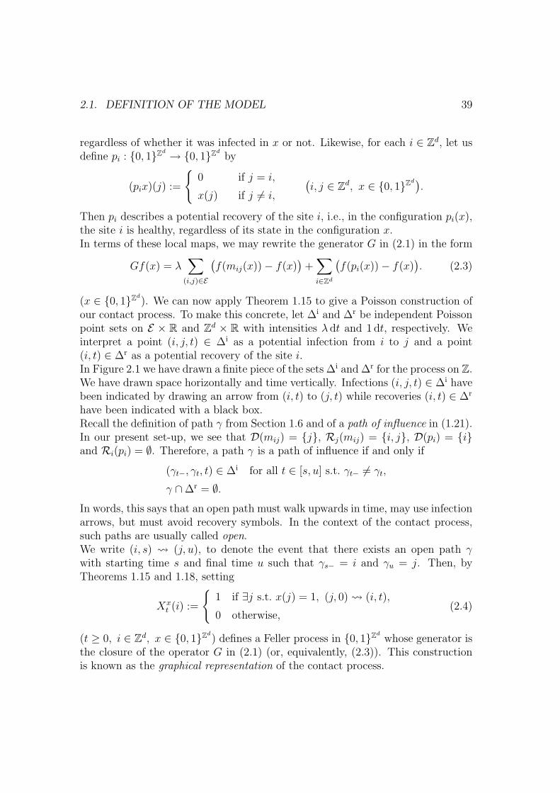
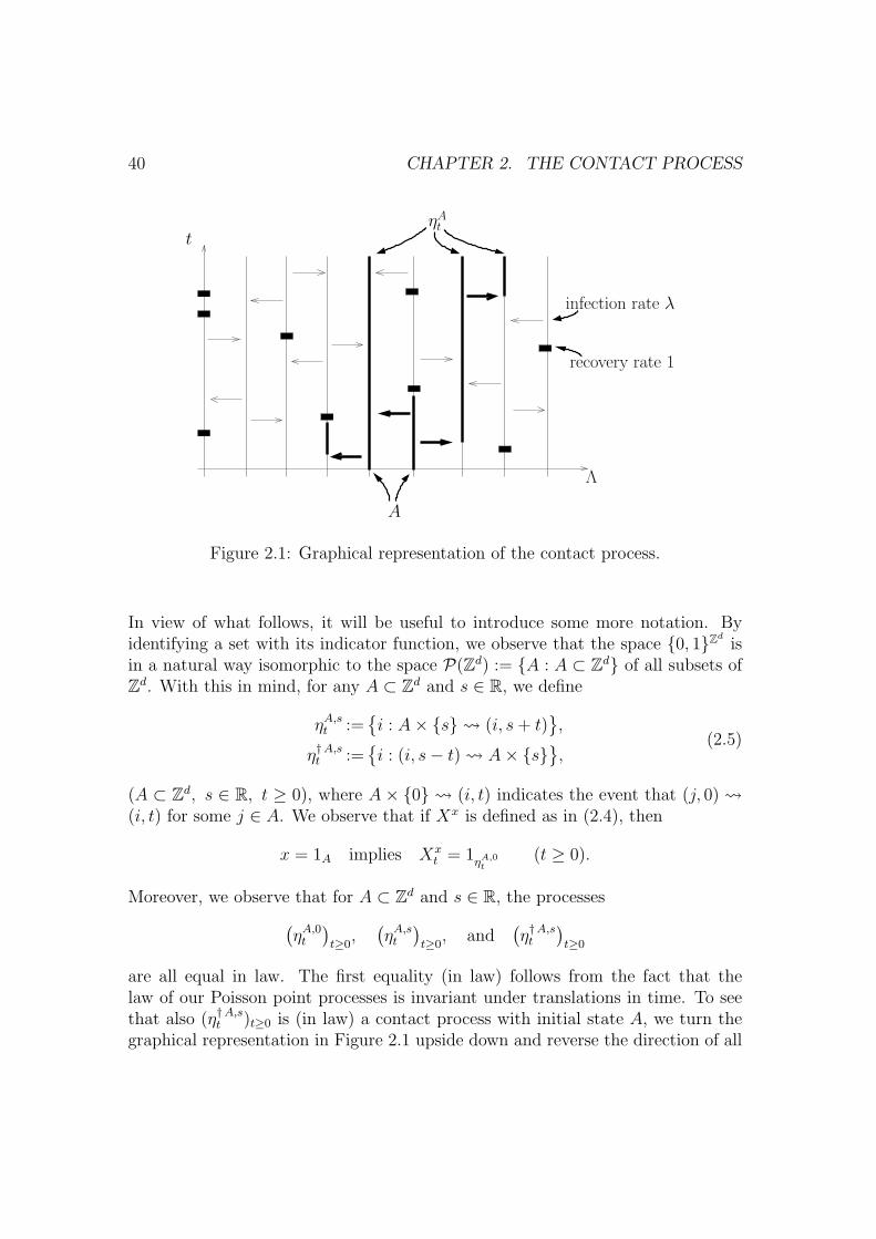
our contact process. To make this concrete, let ∆i and ∆r be independent Poissonpoint sets on E × R and Zd × R with intensities λ dt and 1 dt, respectively. Weinterpret a point (i, j, t) ∈ ∆i as a potential infection from i to j and a point(i, t) ∈ ∆r as a potential recovery of the site i.In Figure 2.1 we have drawn a finite piece of the sets ∆i and ∆r for the process on Z.We have drawn space horizontally and time vertically. Infections (i, j, t) ∈ ∆i havebeen indicated by drawing an arrow from (i, t) to (j, t) while recoveries (i, t) ∈ ∆r
have been indicated with a black box.Recall the definition of path γ from Section 1.6 and of a path of influence in (1.21).In our present set-up, we see that D(mij) = j, Rj(mij) = i, j, D(pi) = iand Ri(pi) = ∅. Therefore, a path γ is a path of influence if and only if
(γt−, γt, t) ∈ ∆i for all t ∈ [s, u] s.t. γt− 6= γt,
γ ∩∆r = ∅.
In words, this says that an open path must walk upwards in time, may use infectionarrows, but must avoid recovery symbols. In the context of the contact process,such paths are usually called open.We write (i, s) (j, u), to denote the event that there exists an open path γwith starting time s and final time u such that γs− = i and γu = j. Then, byTheorems 1.15 and 1.18, setting
Xxt (i) :=
1 if ∃j s.t. x(j) = 1, (j, 0) (i, t),
0 otherwise,(2.4)
(t ≥ 0, i ∈ Zd, x ∈ 0, 1Zd) defines a Feller process in 0, 1Zd
whose generator isthe closure of the operator G in (2.1) (or, equivalently, (2.3)). This constructionis known as the graphical representation of the contact process.
40 CHAPTER 2. THE CONTACT PROCESS
t
Λ
A
ηAt
infection rate λ
recovery rate 1
Figure 2.1: Graphical representation of the contact process.
In view of what follows, it will be useful to introduce some more notation. Byidentifying a set with its indicator function, we observe that the space 0, 1Zd
isin a natural way isomorphic to the space P(Zd) := A : A ⊂ Zd of all subsets ofZd. With this in mind, for any A ⊂ Zd and s ∈ R, we define
ηA,st :=i : A× s (i, s+ t)
,
η†A,st :=i : (i, s− t) A× s
,
(2.5)
(A ⊂ Zd, s ∈ R, t ≥ 0), where A× 0 (i, t) indicates the event that (j, 0) (i, t) for some j ∈ A. We observe that if Xx is defined as in (2.4), then
x = 1A implies Xxt = 1ηA,0
t(t ≥ 0).
Moreover, we observe that for A ⊂ Zd and s ∈ R, the processes(ηA,0t
)t≥0,(ηA,st
)t≥0, and
(η†A,st
)t≥0
are all equal in law. The first equality (in law) follows from the fact that thelaw of our Poisson point processes is invariant under translations in time. To seethat also (η†A,st )t≥0 is (in law) a contact process with initial state A, we turn thegraphical representation in Figure 2.1 upside down and reverse the direction of all

2.1. DEFINITION OF THE MODEL 41
arrows. The resulting picture is again Poisson, with the same rates as before, andwhat used to be an open path from (s, i) to (j, u) is now an open path from (j,−u)to (i,−s).To simplify notation, we write
ηAt := ηA,0t and η†At := η†A,0t (t ≥ 0).
We observe that for any t ≥ 0 and A,B ⊂ Zd,
P[ηA,0t ∩B 6= ∅
]= P
[A× 0 B × t
]= P
[A ∩ η†B,tt 6= ∅
].
This formula remains true if A and B are random sets, independent of the Poissonpoint processes of our graphical representation. This means that we have provedthe following result.
Lemma 2.1 (Duality) Let (ηt)t≥0 and (η†t )t≥0 be independent contact processeson Zd with infection rate λ. Then
P[ηt ∩ η†0 6= ∅
]= P
[η0 ∩ η†t 6= ∅
](t ≥ 0).
This result is especially useful in view of the following fact.
Lemma 2.2 (Distribution determining functions) Let µ, ν be probability lawson P(Zd) such that ∫
µ(dA)1A∩B 6=∅ =
∫ν(dA)1A∩B 6=∅
for all finite nonempty B ⊂ Zd. Then µ = ν.
Proof We start by recalling the Stone-Weierstrass theorem. Let E be a compactmetrizable set. By definition, a subset F of C(E) is an algebra if F is a linearspace, F contains the constant function 1, and f, g ∈ F implies fg ∈ F . We saythat F separates points if for every x, y ∈ E with x 6= y there exists an f ∈ F withf(x) 6= f(y). The Stone-Weierstrass theorem says that if subset F of C(E) is analgebra that separates points, then F is dense in C(E).Let F be the linear span of all functions of the form A 7→ 1A∩B=∅ with B a finitesubset of Zd. Since 1A∩∅=∅ = 1 and 1A∩B=∅1A∩B′=∅ = 1A∩(B∪B′)=∅ we seethat F is an algebra. Since for all A 6= A′ there is a finite B such that 1A∩B=∅ 6=1A′∩B=∅ we see that F separates points, hence by the Stone-Weierstrass theoremF is dense in C(P(Zd)).

42 CHAPTER 2. THE CONTACT PROCESS
It follows from our assumptions that∫µ(dA)1A∩B=∅ =
∫ν(dA)1A∩B=∅
for each finite B ⊂ Zd, hence∫µ(dA)f(A) =
∫ν(dA)f(A) for all f ∈ F and
therefore, since F is dense,∫µ(dA)f(A) =
∫ν(dA)f(A) for all f ∈ C(P(Zd)),
which implies µ = ν.
Exercise 2.3 For each unordered pair i, j of nearest neighbors (i.e., i, j ∈ Zd
such that |i− j| = 1), let us define a local map mij : 0, 1Zd → 0, 1Zdby
(mijx)(k) :=
1 if k ∈ i, j, maxx(i), x(j) = 1,
x(k) otherwise,
(i, j, k ∈ Zd, x ∈ 0, 1Zd). Note that this says that if (x(i), x(j)) = (0, 1) or
(1, 0), then mij changes this into (1, 1); otherwise nothing happens. Show that thegenerator of the contact process can be written in the form (compare (2.3))
Gf(x) = λ∑i,j
(f(mij(x))− f(x)
)+∑i∈Zd
(f(pi(x))− f(x)
), (2.6)
(x ∈ 0, 1Zd), where the sum now runs over all unordered nearest-neighbor pairs.
What kind of graphical representation results from writing the generator in theform (2.6)?
Exercise 2.4 Invent graphical representations for the interacting particle systemson Z with generators (compare (2.1))
G′f(x) =λ∑i∈Z
1x(i)=01x(i−1)+x(i+1)>0(f(xi)− f(x)
)+∑i∈Z
1x(i)=1(f(xi)− f(x)
)and
G′′f(x) =λ∑i∈Z
1x(i)=0(x(i− 1) + x(i+ 1)
)2(f(xi)− f(x)
)+∑i∈Z
1x(i)=1(f(xi)− f(x)
).
2.2. THE SURVIVAL PROBABILITY 43
1
θ(λ)
λcλ
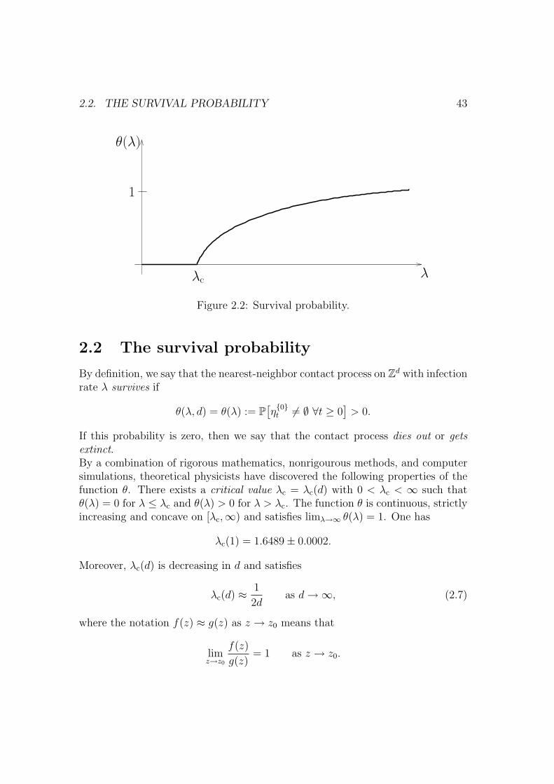
Figure 2.2: Survival probability.
2.2 The survival probability
By definition, we say that the nearest-neighbor contact process on Zd with infectionrate λ survives if
θ(λ, d) = θ(λ) := P[η0t 6= ∅ ∀t ≥ 0
]> 0.
If this probability is zero, then we say that the contact process dies out or getsextinct.By a combination of rigorous mathematics, nonrigourous methods, and computersimulations, theoretical physicists have discovered the following properties of thefunction θ. There exists a critical value λc = λc(d) with 0 < λc < ∞ such thatθ(λ) = 0 for λ ≤ λc and θ(λ) > 0 for λ > λc. The function θ is continuous, strictlyincreasing and concave on [λc,∞) and satisfies limλ→∞ θ(λ) = 1. One has
λc(1) = 1.6489± 0.0002.
Moreover, λc(d) is decreasing in d and satisfies
λc(d) ≈ 1
2das d→∞, (2.7)
where the notation f(z) ≈ g(z) as z → z0 means that
limz→z0
f(z)
g(z)= 1 as z → z0.
44 CHAPTER 2. THE CONTACT PROCESS
The behavior of θ near the critical point is very interesting. One has
θ(λ) ∼ (λ− λc)β as λ ↓ λc, (2.8)
where we write f(z) ∼ g(z) as z → z0 if
limz→z0
log(f(z))
log(g(z))= 1.
The constant β = β(d) is a critical exponent, approximately given by
β(1)∼= 0.276487,β(2)∼= 0.584,β(3)∼= 0.81,β(d) = 1 (d ≥ 4).
In dimensions d 6= 4, it is believed that (2.8) can be strengthened to θ(λ) ≈c(λ− λc)
β for some 0 < c <∞.Below, we will prove some of the easier properties of the function θ, such as mono-tonicity, the existence of a critical parameter λc, and the fact that θ is right-continuous everywhere and left-continuous everywhere except possibly at the crit-ical point λc. Proving that θ is left-continuous at λc, which by our previous remarksis equivalent to the statement that θ(λc) = 0, kept probabilists occupied for some15 years, untill Bezuidenhout and Grimmett proved this in their celebrated paper[BG90]. Quite recently, it has been proved that (2.8) holds with β = 1 if the dimen-sion d is sufficiently large. The critical behavior in dimensions d = 1, 2, 3 remainsvery much an unsolved problem. Physicists come to their prediction (2.8) using(nonrigorous) renormalization group arguments, where critical exponents can berelated to eigenvectors of linearized renormalization transformations near a fixedpoint. Mathematically, there are big problems even defining these renormalizationtransformations rigorously, let alone studying them.In dimension d = 1 it is known rigorously that 1.539 < λc < 1.943 [ZG88, Lig95].For bounds in higher dimensions (including a proof of (2.7)), see [Lig85]. As faras I know, nobody has any idea how to prove that θ is concave on [λc,∞).
Lemma 2.5 (Survival versus extinction) If the contact process survives, then
P[ηAt 6= ∅ ∀t ≥ 0
]> 0 (2.9)
for each finite nonempty A ⊂ Zd. If the contact process dies out, then this proba-bility is zero for each finite nonempty A ⊂ Zd.

2.2. THE SURVIVAL PROBABILITY 45
Proof Let A be finite and nonempty. For obvious reasons we also denote theprobability in (2.9) by
P[(A× 0) ∞
].
Now choose any i ∈ A. Then
P[(0, 0) ∞
]= P
[(i, 0) ∞
]≤ P
[(A× 0) ∞
]= P
[∃j ∈ A s.t. (j, 0) ∞
]≤∑j∈A
P[(j, 0) ∞
]= |A|P
[(0, 0) ∞
],
where we have used translation invariance and |A| denotes the number of elementsin A.
In this and the next section, we will prove the following result.
Theorem 2.6 (Critical infection rate) For each d ≥ 1 there exists a λc = λc(d)with 0 < λc < ∞ such that the nearest-neighbour contact process on Zd withinfection rate λ survives for λ > λc and dies out for λ < λc.
Note that this theorem says nothing about survival or extinction if λ = λc(d).
As a first step towards Theorem 2.6, we prove the following fact.
Lemma 2.7 (Monotone coupling) Let (ηt)t≥0 and (η′t)t≥0 be contact processeson Zd with infection rates 0 ≤ λ ≤ λ′ and deterministic initial states η0 = A andη′0 = A′ satisfying A ⊂ A′. Then (ηt)t≥0 and (η′t)t≥0 can be coupled such that
ηt ⊂ η′t (t ≥ 0).
In particular, survival of the contact process with infection rate λ implies survivalof the contact process with infection rate λ′.
Proof Let 0 ≤ λ ≤ λ′. Let ∆i and ∆i be independent Poisson point sets on E ×Rwith intensities λ dt and (λ′ − λ) dt, respectively, and let ∆r be a Poisson pointset on Zd × R with intensity 1 dt, independent of ∆i and ∆i. Then ∆i ∪ ∆i is aPoisson point set on E × R with intensity λ′ dt. We interpret points in ∆i and ∆i
as infection arrows and points in ∆r as recovery symbols. We let indicate thepresence of an open path that may use infection arrows from ∆i only and we write ′ to indicate the presence of an open path that may use infection arrows from∆i ∪ ∆i. Then
ηt = i : A× 0 (i, t) ⊂ i : A′ × 0 ′ (i, t) = η′t (t ≥ 0)
since A ⊂ A′ and the process (η′t)t≥0 has more arrows at its disposal.
46 CHAPTER 2. THE CONTACT PROCESS
2.3 Extinction
It follows from Lemma 2.7 that the function λ 7→ θ(λ) is nondecreasing and hence,for each d ≥ 1, there exists a 0 ≤ λc(d) ≤ ∞ such that the nearest-neighbourcontact process on Zd with infection rate λ survives for λ > λc and dies out forλ < λc. To prove Theorem 2.6, we must show that 0 < λc(d) < ∞. We start byproving a the lower bound on λc, which is easiest.
Lemma 2.8 (Exponential bound) For each finite A ⊂ Zd, one has
E[|ηAt |
]≤ |A|e(2dλ−1)t (t ≥ 0). (2.10)
Proof For the contact process, the constant K from (1.23) is given by K = 2dλ−1.Therefore, the statement is a direct consequence of Lemma 1.13.
Lemma 2.8 has the following consequence.
Corollary 2.9 (Lower bound on critical infection rate) The critical infec-tion rate of the nearest-neighbour contact process on Zd satisfies 1
2d≤ λc.
Proof By (2.10), for each λ < 12d
,
P[ηAt 6= ∅
]≤ E
[|ηAt |
]−→t→∞
0
for each finite A ⊂ Zd.
In order to finish the proof of Theorem 2.6 we need to show that λc < ∞. As apreparation for this, in the next section, we will start by studying a closely relatedproblem. Before we do this, we apply the techniques developed so far to prove thatthe function θ(λ, d) is nondecreasing and right-continuity. Left-continuity, except(possibly) in the critical point λc, will be proved in Proposition 2.22 below.
Proposition 2.10 (Monotonicty and right-continuity) The survival proba-bility θ(λ, d) is nondecreasing and right-continuous in λ, and nondecreasing in d.
Proof The fact that θ(λ, d) is nondecreasing in λ follows from Lemma 2.7. Thefact that θ(λ, d) is nondecreasing in d can be proved in a similar way, since ifd ≤ d′, then we may view Zd as a subset of Zd′ and observe that if there is an openpath that stays in Zd, then certainly there is an open path in Zd′ .To prove right continuity of θ(λ, d) in λ, we will improve the coupling used in theproof of Lemma 2.7 in such a way that we can define contact processes for anyvalue of the infection rate on the same probability space. To this aim, consider

2.4. ORIENTED PERCOLATION 47
the space E ×R× [0,∞) whose elements are triples ((i, j), t, κ) with (i, j) ∈ E and
t ∈ R, κ ≥ 0, and let ∆i
be a Poisson point set on this set with indensity dtdκ.Then, for each λ ≥ 0,
∆iλ :=
(((i, j), t
): ∃((i, j), t, κ
)∈ ∆
iwith κ ≤ λ
.
is a Poisson point sets on E × R with intensity λdt. Let ∆r be an independentPoisson point set on Zd×R with intensity dt and write λ to indicate the presenceof an open path in the graphical representations defined by (∆i
λ,∆r). Another way
of saying this is that a point ((i, j), t, κ) ∈ ∆i
indicates the presence of an arrowwhich has a value κ attached to it, and λ indicates the presence of a path thatmay use only arrows with values κ ≤ λ. Let λn ↓ λ∗. Then we claim that
limλn↓λ∗
θ(λn) = limλ↓λ∗
P[(0, 0) λ ∞] = P[(0, 0) λ ∞ ∀λ > λ∗]
!= P[(0, 0) λ∗ ∞] = θ(λ∗).
The equality!
= needs some explanation. It is obvious that (0, 0) λ∗ ∞ implies(0, 0) λ ∞ ∀λ > λ∗. On the other hand, if (0, 0) 6 λ∗ ∞ then by Lemma 2.8
I :=
(i, t) ∈ Zd × R : (0, 0) λ∗ (i, t)
is a compact subset of Zd ×R, such that each each infection ends somewhere in arecovery sign, and all infection arrows starting in I and ending somewhere outsideI have a value strictly larger than λ∗. Since there are only finitely many arrowswith values κ ∈ (λ∗, 2λ∗) starting in I and ending somewhere outside I, we knowthat there is some λ′ > λ∗ such that all arrows starting in I and ending somewhereoutside I have a value larger than λ′, i.e., we know that (0, 0) 6 λ′ ∞ for someλ′ > λ∗.
2.4 Oriented percolation
In order to prepare for the proof that the critical infection rate of the contactprocess is finite, in the present section, we will study oriented (or directed) bondpercolation on Zd. For i, j ∈ Zd, we write i ≤ j if i = (i1, . . . , id) and j =(j1, . . . , jd) satisfy ik ≤ jk for all k = 1, . . . , d. Let
A :=
(i, j) : i, j ∈ Zd, i ≤ j, |i− j| = 1.
We view Zd as an infinite directed graph, where elements (i, j) ∈ A representarrows (or directed bonds) between neighbouring sites. Note that all arrows point‘upwards’ in the sense of the natural order on Zd.

48 CHAPTER 2. THE CONTACT PROCESS
Now fix some percolation parameter p ∈ [0, 1] and let (ω(i,j))(i,j)∈A be a collectionof i.i.d. Bernoulli random variables with P[ω(i,j) = 1] = p. We say that there isan open path from a site i ∈ Zd to j ∈ Zd if there exist n ≥ 0 and a functionγ : 0, . . . , n → Zd such that
(γ(k − 1), γ(k)) ∈ A and ω(γ(k−1),γ(k)) = 1 (k = 1, . . . , n).
We denote the presence of an open path by . Note that open paths must walkupwards in the sense of the order on Zd. We write 0 ∞ to indicate the existenceof an infinite open path starting at the origin 0 ∈ Zd.
Theorem 2.11 (Critical percolation parameter) For oriented percolation indimensions d ≥ 2 there exists a critical parameter pc = pc(d) with 0 < pc < 1 suchthat P[0 ∞] = 0 for p < pc and P[0 ∞] > 0 for p > pc.
Proof The existence of a critical parameter pc ∈ [0, 1] follows from a monotonecoupling argument like the one we used in the proof of Lemma 2.7. To prove that0 < pc, let Nn denote the number of open paths of length n starting in 0. Sincethere are dn different upward paths of length n starting at the origin, and eachpath has probability pn to be open, we see that
E[ ∞∑n=1
Nn
]=∞∑n=1
dnpn <∞ (p < 1/d)
This shows that∑∞
n=1Nn <∞ a.s., hence P[0 ∞] = 0 if p < 1/d, and therefore
1
d≤ pc(d).
To prove that pc(d) < 1 for d ≥ 2 it suffices to consider the case d = 2, for we mayview Z2 as a subset of Zd (d ≥ 3) and then, if there is an open path that stays inZ2, then certainly there is an open path in Zd. (Note, by the way, that in d = 1one has P[0 ∞] = 0 for all p < 1 hence pc(1) = 1.)
We claim that
pc(2) ≤ 8
9. (2.11)
To prove this, we use a Peierls argument, named after R. Peierls who used a similarargument in 1936 for the Ising model [Pei36]. In Figure 2.3, we have drawn a pieceof Z2. Open arrows are drawn in black; closed arrows are not drawn. Sites i ∈ Z2
such that 0 i are indicated in black. These sites are called wet. Consider thedual lattice
Z2 := (n+ 12,m+ 1
2) : (n,m) ∈ Z2.

2.4. ORIENTED PERCOLATION 49
Figure 2.3: Peierls argument for oriented percolation.
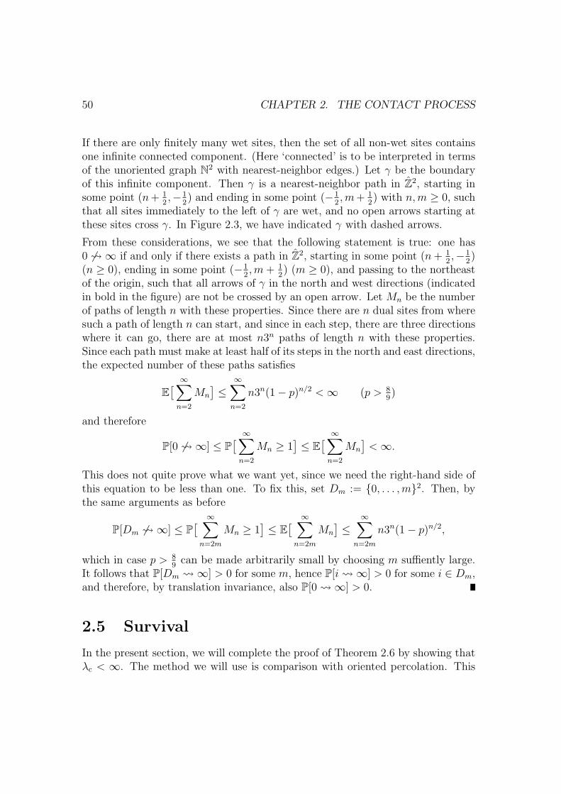
50 CHAPTER 2. THE CONTACT PROCESS
If there are only finitely many wet sites, then the set of all non-wet sites containsone infinite connected component. (Here ‘connected’ is to be interpreted in termsof the unoriented graph N2 with nearest-neighbor edges.) Let γ be the boundaryof this infinite component. Then γ is a nearest-neighbor path in Z2, starting insome point (n+ 1
2,−1
2) and ending in some point (−1
2,m+ 1
2) with n,m ≥ 0, such
that all sites immediately to the left of γ are wet, and no open arrows starting atthese sites cross γ. In Figure 2.3, we have indicated γ with dashed arrows.
From these considerations, we see that the following statement is true: one has0 6 ∞ if and only if there exists a path in Z2, starting in some point (n+ 1
2,−1
2)
(n ≥ 0), ending in some point (−12,m+ 1
2) (m ≥ 0), and passing to the northeast
of the origin, such that all arrows of γ in the north and west directions (indicatedin bold in the figure) are not be crossed by an open arrow. Let Mn be the numberof paths of length n with these properties. Since there are n dual sites from wheresuch a path of length n can start, and since in each step, there are three directionswhere it can go, there are at most n3n paths of length n with these properties.Since each path must make at least half of its steps in the north and east directions,the expected number of these paths satisfies
E[ ∞∑n=2
Mn
]≤
∞∑n=2
n3n(1− p)n/2 <∞ (p > 89)
and therefore
P[0 6 ∞] ≤ P[ ∞∑n=2
Mn ≥ 1]≤ E
[ ∞∑n=2
Mn
]<∞.
This does not quite prove what we want yet, since we need the right-hand side ofthis equation to be less than one. To fix this, set Dm := 0, . . . ,m2. Then, bythe same arguments as before
P[Dm 6 ∞] ≤ P[ ∞∑n=2m
Mn ≥ 1]≤ E
[ ∞∑n=2m
Mn
]≤
∞∑n=2m
n3n(1− p)n/2,
which in case p > 89
can be made arbitrarily small by choosing m suffiently large.It follows that P[Dm ∞] > 0 for some m, hence P[i ∞] > 0 for some i ∈ Dm,and therefore, by translation invariance, also P[0 ∞] > 0.
2.5 Survival
In the present section, we will complete the proof of Theorem 2.6 by showing thatλc < ∞. The method we will use is comparison with oriented percolation. This
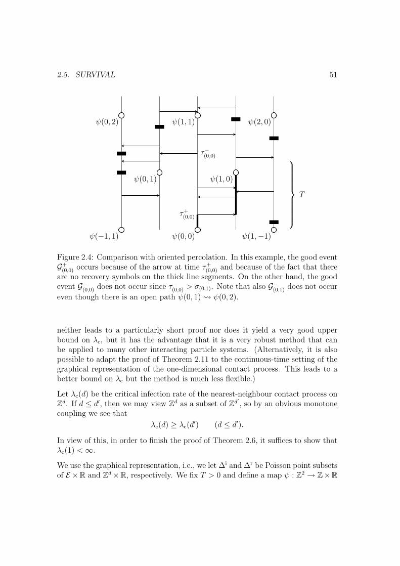
2.5. SURVIVAL 51
ψ(−1, 1) ψ(0, 0) ψ(1,−1)
ψ(0, 1) ψ(1, 0)
ψ(0, 2) ψ(1, 1) ψ(2, 0)
τ+(0,0)
τ−(0,0) T
Figure 2.4: Comparison with oriented percolation. In this example, the good eventG+
(0,0) occurs because of the arrow at time τ+(0,0) and because of the fact that there
are no recovery symbols on the thick line segments. On the other hand, the goodevent G−(0,0) does not occur since τ−(0,0) > σ(0,1). Note that also G−(0,1) does not occur
even though there is an open path ψ(0, 1) ψ(0, 2).
neither leads to a particularly short proof nor does it yield a very good upperbound on λc, but it has the advantage that it is a very robust method that canbe applied to many other interacting particle systems. (Alternatively, it is alsopossible to adapt the proof of Theorem 2.11 to the continuous-time setting of thegraphical representation of the one-dimensional contact process. This leads to abetter bound on λc but the method is much less flexible.)
Let λc(d) be the critical infection rate of the nearest-neighbour contact process onZd. If d ≤ d′, then we may view Zd as a subset of Zd′ , so by an obvious monotonecoupling we see that
λc(d) ≥ λc(d′) (d ≤ d′).
In view of this, in order to finish the proof of Theorem 2.6, it suffices to show thatλc(1) <∞.
We use the graphical representation, i.e., we let ∆i and ∆r be Poisson point subsetsof E ×R and Zd×R, respectively. We fix T > 0 and define a map ψ : Z2 → Z×R

52 CHAPTER 2. THE CONTACT PROCESS
byψ(i) =
(κi, σi
):=(i1 − i2, T (i1 + i2)
) (i = (i1, i2) ∈ Z2
).
Recall from the previous section the definition of the set A of arrows on Zd. Wewish to define a collection (ω(i,j))(i,j)∈A of Bernoulli random variables such that
ω(i,j) = 1 implies (κi, σi) (κj, σj)((i, j) ∈ A
).
For each i ∈ Z2 we let
τ−i := inft ≥ σi : (κi, κi − 1, t) ∈ ∆i,
τ+i := inf
t ≥ σi : (κi, κi + 1, t) ∈ ∆i,
denote the times of the first arrows out of i to the left and right, and we definethe ‘good events’
G−i :=τ−i < σi + T,
(κi × (σi, τ
−i ))∩∆r = ∅,(
κi − 1 × (τ−i , σi + T ))∩∆r = ∅
,
G+i :=
τ+i < σi + T,
(κi × (σi, τ
+i ))∩∆r = ∅,(
κi + 1 × (τ+i , σi + T )
)∩∆r = ∅
.
We observe that the event G±i implies that (κi, σi) (κi ± 1, σi + T ) via an openpath that stays in κi, κi ± 1. In view of this, we set
ω((i1, i2), (i1 + 1, i2)) := 1G+i,
ω((i1, i2), (i1, i2 + 1)) := 1G−i.
Then ω(i,j) = 1 implies the existence of an open path in the graphical representationfor the contact process from (κi, σi) to (κj, σj) (with (i, j) ∈ A), hence if we usethe random variables (ω(i,j))(i,j)∈A to define oriented percolation on Z2 in the usualway, then:
i j in the oriented percolation on Z2 defined by the random variables(ω(i,j))(i,j)∈A implies (κi, σi) (κi, σi) in the graphical representationfor the contact process.
We observe that
p := P[ω(i,j) = 1] = P(G±i ) = (1− e−λT )e−T((i, j) ∈ A
). (2.12)
For λ sufficiently large, by a suitable choice of T , we can make p as close to oneas we wish. We would like to conclude from this that P[(0, 0) ∞] > 0 for the
2.6. K-DEPENDENCE 53
oriented percolation defined by the ω(i,j)’s, and therefore also P[(0, 0) ∞] > 0for the contact process. Unfortunately, the random variables (ω(i,j))(i,j)∈A are notindependent, and therefore Theorem 2.11 is not applicable. To fix this problem,we need a bit more theory. In the next section, we will introduce the concept ofk-dependence. As will be clear from the definition there, the (ω(i,j))(i,j)∈A are k-dependent for some suitable k, so by applying Theorem 2.12 from the next sectionwe can estimate them from below by an independent collection of Bernoulli randomvariables (ω(i,j))(i,j)∈A whose succes probability p can be made arbitrarily close toone, so we are done.
2.6 K-dependence
By definition, for k ≥ 0, one says that a collection (Xi)i∈Zd of random variables,indexed by the integer square lattice, is k-dependent if for any A,B ⊂ Zd with
inf|i− j| : i ∈ A, j ∈ B > k,
the collections of random variables (Xi)i∈A and (Xj)j∈B are independent of eachother. Note that in particular, 0-dependence means independence.
The most important property associated with k-dependence is that a collection ofk-dependent Bernoulli random variables with success probability p can be stochas-tically estimated from below by a collection of independent Bernoulli random vari-ables with a success probability p that has the property that p→ 1 as p→ 1. It isa bit unfortunate that the term ‘k-dependence’ as it is standardly used explicity(and only) refers to random variables on Zd, while in fact, as the next theoremshows, for the property just mentioned the precise spatial structure is not veryimportant. The next theorem is taken from [Lig99, Thm B26], who in turn cites[LSS97].
Theorem 2.12 (K-dependence) Let Λ be a countable set and let p ∈ (0, 1),K < ∞. Assume that (χi)i∈Λ are Bernoulli random variables with P [χi = 1] ≥ p(i ∈ Λ), such that for each i ∈ Λ there exists a ∆i ⊂ Λ with i ∈ ∆i and |∆i| ≤ K,such that
χi is independent of (χj)j∈Λ\∆i.
Then it is possible to couple (χi)i∈Λ to a collection of independent Bernoulli randomvariables (χi)i∈Λ with
P [χi = 1] = p :=(1− (1− p)1/K
)2, (2.13)
in such a way that χi ≤ χi for all i ∈ Λ.

54 CHAPTER 2. THE CONTACT PROCESS
Proof of Theorem 2.12 Since we can always choose some arbitrary denumerationof Λ, we may assume that Λ = N. Our strategy will be as follows. We will choose0, 1-valued random variables (ψi)i∈Λ with P [ψi = 1] = r, independent of eachother and of the (χi)i∈N, and put
χ′i := ψiχi (i ∈ N). (2.14)
Note that the (χ′i)i∈N are a ‘thinned out’ version of the (χi)i∈N. In particular,χ′i ≤ χi (i ∈ N). We will show that for an appropriate choice of r,
P [χ′n = 1 |χ′0, . . . , χ′n−1] ≥ p (2.15)
for all n ≥ 0, and we will show that this implies that the (χ′i)i∈N can be coupledto independent (χi)i∈Λ as in (2.13) in such a way that χi ≤ χ′i ≤ χi (i ∈ N).We start with the latter claim. Imagine that (2.15) holds. Set
p′n(ε0, . . . , εn−1) := P [χ′n = 1 |χ′0 = ε0, . . . , χ′n−1 = εn−1] (2.16)
whenever P [χ′0 = ε0, . . . , χ′n−1 = εn−1] > 0. Let (Un)n∈N be independent, uniformly
distributed [0, 1]-valued random variables. Set
χn := 1Un < p (n ∈ N) (2.17)
and define inductively
χ′n := 1Un < p′n(χ′0, . . . , χ′n−1) (i ∈ N). (2.18)
ThenP [χ′n = εn, . . . , χ
′0 = ε0] = pn(ε0, . . . , εn−1) · · · p0. (2.19)
This shows that these new χ′n’s have the same distribution as the old ones, andthey are coupled to χi’s as in (2.13) in such a way that χi ≤ χ′i.What makes life complicated is that (2.15) does not always hold for the original(χi)i∈N, which is why we have to work with the thinned variables (χ′i)i∈N.1 Weobserve that
P [χ′n = 1 |χ′0 = ε0, . . . , χ′n−1 = εn−1] = rP [χn = 1 |χ′0 = ε0, . . . , χ
′n−1 = εn−1].
(2.20)
1Indeed, let (φn)n≥0 be independent 0, 1-valued random variables with P [φn = 1] =√p for
some p < 1, and put χn := φnφn+1. Then the (χn)n≥0 are 1-dependent with P [χn = 1] = p, butP [χn = 1|χn−1 = 0, χn−2 = 1] = 0.

2.6. K-DEPENDENCE 55
We will prove by induction that for an appropriate choice of r,
P [χn = 0 |χ′0 = ε0, . . . , χ′n−1 = εn−1] ≤ 1− r. (2.21)
Note that this is true for n = 0 provided that r ≤ p. Let us put
E0 := i ∈ ∆n : 0 ≤ i ≤ n− 1, εi = 0,E1 := i ∈ ∆n : 0 ≤ i ≤ n− 1, εi = 1,F := i 6∈ ∆n : 0 ≤ i ≤ n− 1.
(2.22)
Then
P [χn = 0 |χ′0 = ε0, . . . , χ′n−1 = εn−1]
= P[χn = 0
∣∣χ′i = 0 ∀i ∈ E0, χi = 1 = ψi ∀i ∈ E1, χ′i = εi ∀i ∈ F
]= P
[χn = 0
∣∣χ′i = 0 ∀i ∈ E0, χi = 1 ∀i ∈ E1, χ′i = εi ∀i ∈ F
]=P[χn = 0, χ′i = 0 ∀i ∈ E0, χi = 1 ∀i ∈ E1, χ
′i = εi ∀i ∈ F
]P[χ′i = 0 ∀i ∈ E0, χi = 1 ∀i ∈ E1, χ′i = εi ∀i ∈ F
]≤
P[χn = 0, χ′i = εi ∀i ∈ F
]P[ψi = 0 ∀i ∈ E0, χi = 1 ∀i ∈ E1, χ′i = εi ∀i ∈ F
]=
P[χn = 0
∣∣χ′i = εi ∀i ∈ F]
P[ψi = 0 ∀i ∈ E0, χi = 1 ∀i ∈ E1
∣∣χ′i = εi ∀i ∈ F]
≤ 1− p(1− r)|E0|P
[χi = 1 ∀i ∈ E1
∣∣χ′i = εi ∀i ∈ F] ≤ 1− p
(1− r)|E0| r|E1|,
(2.23)
where in the last step we have used K-dependence and the (nontrivial) fact that
P[χi = 1 ∀i ∈ E1
∣∣χ′i = εi ∀i ∈ F]≥ r|E1|. (2.24)
We claim that (2.24) is a consequence of the induction hypothesis (2.21). Indeed,we may assume that the induction hypothesis (2.21) holds regardless of the or-dering of the first n elements, so without loss of generality we may assume thatE1 = n−1, . . . ,m and F = m−1, . . . , 0, for some m. Then the left-hand sideof (2.24) may be written as
n−1∏k=m
P[χk = 1
∣∣χi = 1 ∀m ≤ i < k, χ′i = εi ∀0 ≤ i < m]
=n−1∏k=m
P[χk = 1
∣∣χ′i = 1 ∀m ≤ i < k, χ′i = εi ∀0 ≤ i < m]≥ rn−m.
(2.25)

56 CHAPTER 2. THE CONTACT PROCESS
If we assume moreover that r ≥ 12, then r|E1| ≥ (1 − r)|E1| and therefore the
right-hand side of (2.23) can be further estimated as
1− p(1− r)|E0| r|E1|
≤ 1− p(1− r)|∆n∩0,...,n−1| ≤
1− p(1− r)K−1
. (2.26)
We see that in order for our proof to work, we need 12≤ r ≤ p and
1− p(1− r)K−1
≤ 1− r. (2.27)
In particular, choosing r = 1− (1− p)1/K yields equality in (2.27). Having proved(2.21), we see by (2.20) that (2.15) holds provided that we put p := r2.
Exercise 2.13 Combine formulas (2.11), (2.12) and (2.13) to derive an explicitupper bound on the critical infection rate λc of the one-dimensional contact pro-cess.
2.7 The upper invariant law
For any Feller semigroup (Pt)t≥0 on C(E), where E is some compact metrizablespace, we say that a probability measure µ on E is an invariant law if∫
µ(dx)Pt(x, · ) = µ (t ≥ 0).
Note that this says that for the associated Feller process, P[X0 ∈ · ] = µ impliesP[Xt ∈ · ] = µ for each t ≥ 0. If µ is an invariant law, then it is possible toconstruct a stationary process (Xt)t∈R that is also defined for negative times, suchthat P[Xt ∈ · ] = µ for all t ∈ R and (Xt)t∈R is a Feller process associated with(Pt)t≥0, where we generalize (1.11) in the obvious way to negative times.
Using our graphical representation of the contact process, we define
ηt :=i ∈ Zd : −∞ (i, t)
(t ∈ R).
where −∞ (i, t) indicates the presence of an open path γ : (−∞, t]→ Zd. (Notethat so far, we have only defined paths with finite starting and ending times butthe definition of an (open) path can easily be extended to allow for infinite paths.)Using the independence of restrictions of Poisson point processes to disjoint partsof space, we see that
P[ηu ∈ ·
∣∣ (ηs)s≤t] = Pu−t(ηt, · ) a.s. (t ≤ u),

2.7. THE UPPER INVARIANT LAW 57
hence (ηt)t∈R is a stationary contact process and its law at any given time
ν := P[ηt ∈ ·
](t ∈ R)
is an invariant law of the contact process. We call ν the upper invariant law ofthe contact process (with given infection rate). As we will see in a moment, in acertain sense, it is the ‘largest’ invariant law of our process.
By definition, we say that a function f : 0, 1Zdis monotone if f(x) ≤ f(y) for
all x ≤ y.
Proposition 2.14 (Stochastic order) Let µ, ν be probability laws on 0, 1Zd.
Then the following statements are equivalent:
(i)∫µ(dx)f(x) ≤
∫ν(dx)f(x) ∀ monotone f ∈ C(0, 1Zd
),
(ii)∫µ(dx)f(x) ≤
∫ν(dx)f(x) ∀ monotone f ∈ B(0, 1Zd
),
(iii) It is possible to couple random variables X, Y with laws µ = P [X ∈ · ]and ν = P [Y ∈ · ] in such a way that X ≤ Y .
Proof The implications (iii)⇒(ii)⇒(i) are trivial. For the nontrivial implication(i)⇒(iii) (which we will never actually need to use), see [Lig85, Theorem II.2.4].
Remark The statements of Proposition 2.14 are not restricted to probability lawson 0, 1Zd
. Analogue statements hold for probability laws on R (equipped withthe usual order) or more generally Rn, as well as for other metric spaces on whichan order is defined that is somehow ‘compatible’ with the topology; see [Lig85,Theorem II.2.4].
If probability laws µ, ν on 0, 1Zdsatisfy the equivalent conditions (i)–(iii) from
Proposition 2.14, then we say that µ and ν are stochastically ordered and we write2
µ ≤ ν.
Lemma 2.15 (Upper invariant law) Let ν be the upper invariant law of thecontact process and let ν be any other invariant law. Then ν ≤ ν in the stochasticorder.
2This notation may look a bit confusing at first sight, since, if µ, ν are probability measureson any measurable space (Ω,F), then one might interpret µ ≤ ν in a pointwise sense, i.e., inthe sense that µ(A) ≤ ν(A) for all A ∈ F . In practice, this does not lead to confusion, sincepointwise inequality for probability measures is a very uninteresting property. Indeed, it is easyto check that probability measures µ, ν satisfy µ ≤ ν in a pointwise sense if and only if µ = ν.

58 CHAPTER 2. THE CONTACT PROCESS
Proof Let A be a random variable, taking values in P(Zd), with law P[A ∈ · ] = ν,and assume that A is independent of the Poisson point processes used in ourgraphical representation. Then, since ν is an invariant law, we have ν = P[ηAt ∈ · ]for all t ≥ 0. Since the random variables
(ηAt , ηt),
take values in the compact space P(Zd)2, their laws are automatically tight, hencewe can select a subsequence tn → ∞ such that the (ηAtn , ηtn) converge weakly inlaw to some limiting random variable (η1, η2), say, where η1 has the law ν, η2 hasthe law ν, and moreover
P[i ∈ η1, i /∈ η2] = limn→∞
P[i ∈ ηAtn , i 6∈ ηtn ] = limn→∞
P[i ∈ ηA,−tn0 , i 6∈ η0]
≤ limn→∞
P[Zd × −tn (i, 0), −∞ 6 (i, 0)] = 0 (i ∈ Zd),
where we have used that the events Zd × −tn (i, 0) decrease monotonicallyto the event −∞ (i, 0), hence the events Zd × −tn (i, 0), −∞ 6 (i, 0)decrease monotonically to the empty set. We conclude that η1 ⊂ η2 a.s., henceν ≤ ν in the stochastic order.
By definition, we say that a probability law µ on P(Zd) is nontrivial if
µ(∅) = 0,
i.e., if µ gives zero probability to the configuration in which all sites are healthy.
Lemma 2.16 (Survival and the upper invariant law) For the contact processon Zd with infection rate λ ≥ 0, the following statements are equivalent:
(i) The contact process survives, i.e., θ(λ, d) > 0.
(ii) The upper invariant law ν is nontrivial.
(iii) There exists a nontrivial invariant law.
Moreover, if the contact process dies out, then ν = δ∅.
Proof The implication (ii)⇒(iii) is trivial and (iii)⇒(ii) follows from Lemma 2.15.To see that (i) and (ii) are equivalent, we start by observing that by duality, foreach finite B ⊂ Zd∫
ν(dA)1A∩B 6=∅ = P[η0 ∩B 6= ∅]
= P[η†B,0t 6= ∅ ∀t ≥ 0] = P[ηBt 6= ∅ ∀t ≥ 0].(2.28)

2.8. ERGODIC BEHAVIOR 59
Note that by Lemma 2.2, this formula determines the law ν uniquely. In particular,we see that ν = δ∅ if the contact process dies out. On the other hand, if thecontact process survives, then ν 6= δ∅. This is not quite the same as saying that νis nontrivial, but at least it tells us that P[η0 6= ∅] > 0. We observe that
P[ηt 6= ∅
]= P
[ηt 6= ∅
∣∣ η0 6= ∅]P[η0 6= ∅
],
which by the stationarity of η implies that
P[ηt 6= ∅
∣∣ η0 6= ∅]
= 1 (t ≥ 0).
It follows that the conditioned law
ν( · |A : A 6= ∅)
is a nontrivial invariant law for the contact process, hence by the equivalence of(ii) and (iii), we must have that ν is nontrivial.
2.8 Ergodic behavior
We define translation operators Ti : P(Zd)→ P(Zd) by
Ti(A) := j + i : j ∈ A (i ∈ Zd).
Below, we will sometimes also use the notation
Ti(A) = i+ A.
We say that a probability law µ on P(Zd) is homogeneous or translation invariantif µ T−1
i = µ for all i ∈ Zd. A lot of work in the theory of interacting particlesystems is concerned with classifying all invariant laws of a given system, andproving that the system started from certain initial laws converges in law to acertain invariant law. In the context of interacting particle systems, invariant lawsare sometimes also called equilibria or equilibrium laws. If an interacting particlesystem has a unique invariant law, which is the limit law of the process started inany initial state, then it is often said that the system is ergodic.3
3This is not very good terminology since it may lead to confusion with another, more usualconcept of ergodicity. If (Xt)t∈R is a stationary process, for example an interacting particle systemin equilibrium, then by definition (Xt)t∈R is ergodic if the law of (Xt)t∈R gives probability zeroor one to all events that are invariant under time shifts. In fact, if a Markov process is ergodicas defined in the text above, then the corresponding stationary process is ergodic in the sensedefined here, but the converse does not hold in general.
60 CHAPTER 2. THE CONTACT PROCESS
The main aim of the present section is to prove the following result. It seems thisresult is due to Harris [Har76], who in particular seems to have invented the useof Holder’s inequality in the proof of Lemma 2.19. I believe an earlier version ofTheorem 2.17, for a somewhat more limited class of initial laws, was proved by aRussian mathematician, but I forgot who.
Theorem 2.17 (Convergence to upper invariant law) Let (ηt)t≥0 be a con-tact process started in a homogeneus nontrivial initial law P[η0 ∈ · ]. Then
P[ηt ∈ · ] =⇒t→∞
ν,
where ν is the upper invariant law.
We start with two preparatory lemmas.
Lemma 2.18 (Extinction versus unbounded growth) For each finite A ⊂Zd, one has
ηAt = ∅ for some t ≥ 0 or |ηAt | −→t→∞∞ a.s. (2.29)
Proof Define
ρ(A) := P[ηAt 6= ∅ ∀t ≥ 0
](A ⊂ Z2, |A| <∞).
It is not hard to see that for each N ≥ 0 there exists an ε > 0 such that
|A| ≤ N implies ρ(A) ≤ 1− ε. (2.30)
We first argue why it is plausible that this implies (2.29) and then give a rigorousproof. Imagine that |ηAt | 6→ ∞. Then, in view of (2.30), the process infinitely oftengets a chance of at least ε to die out, hence eventually it should die out.To make this rigorous, let
AA := ηAt 6= ∅ ∀t ≥ 0 (A ⊂ Z2, |A| <∞).
denote the event that the process (ηAt )t≥0 survives and let Ft be the σ-field gener-ated by the Poisson point processes used in our graphical representation till time t.Then
ρ(ηAt ) = P[AA∣∣Ft] −→
t→∞1AA
a.s., (2.31)
where we have used an elementary result from probability theory which says that ifFn is an increasing sequence of σ-fields and F∞ = σ(
⋃nFn), then limn P[A|Fn] =
P[A|F∞] a.s. for each measurable event A. (See [Loe63, § 29, Complement 10 (b)].)In view of (2.30), formula (2.31) implies (2.29).
2.8. ERGODIC BEHAVIOR 61
Lemma 2.19 (Nonzero intersection) Let (ηt)t≥0 be a contact process startedin a homogeneus nontrivial initial law P[η0 ∈ · ]. Then for each s, ε > 0 thereexists an N ≥ 1 such that for any subset A ⊂ Zd
|A| ≥ N implies P[A ∩ ηs 6= ∅
]≥ 1− ε.
Proof By duality (Lemma 2.1)
P[A ∩ ηs 6= ∅
]= P
[ηAs ∩ η0 6= ∅
]where η0 is independent of the graphical representation used to define ηAs . SetΛM := −M, . . . ,Md. It is not hard to see that each set A ⊂ Zd with |A| ≥ Ncontains a subset A′ ⊂ A with |A′| ≥ N/|ΛM | such that the sets
i+ ΛM : i ∈ A′
are disjoint, where as before we define i + ΛM := i + j : j ∈ ΛM. Write i+ΛM
to indicate the presence of an open path that stays in i+ ΛM and set
ηi (M)s :=
j ∈ Zd : (i, 0) i+ΛM
(j, s).
Then, using Holder’s inequality4 in the inequality marked with an exclamationmark, we have
P[ηAs ∩ η0 = ∅
]=
∫P[η0 ∈ dB]P
[ηAs ∩B = ∅
]≤∫
P[η0 ∈ dB]P[ ⋃i∈A′
ηi (M)s ∩B = ∅
]=
∫P[η0 ∈ dB]
∏i∈A′
P[ηi (M)s ∩B = ∅
]!
≤∏i∈A′
(∫P[η0 ∈ dB]P
[ηi (M)s ∩B = ∅
]|A′|)1/|A′|
=∏i∈A′
(∫P[η0 ∈ dB]P
[η0 (M)s ∩B = ∅
]|A′|)1/|A′|
=
∫P[η0 ∈ dB]P
[η0 (M)s ∩B = ∅
]|A′|,
where we have used the homogeneity of P[η0 ∈ · ] in the one but last equality. Ourarguments so far show that |A| ≥ N implies that
P[A ∩ ηs = ∅
]≤∫
P[η0 ∈ dB]P[η0 (M)s ∩B = ∅
]N/|ΛM | =: f(N,M).
4Recall that Holder’s inequality says that 1/p + 1/q = 1 implies ‖fg‖1 ≤ ‖f‖p‖g‖q, where‖f‖p := (
∫|f |pdµ)1/p. By induction, this gives ‖
∏ni=1 fi‖1 ≤
∏ni=1 ‖fi‖n.

62 CHAPTER 2. THE CONTACT PROCESS
Here, using the fact that
P[η0 (M)s ∩B = ∅
]< 1 if B ∩ ΛM 6= ∅,
we see that
limN↑∞
f(N,M) =
∫P[η0 ∈ dB]1B∩ΛM =∅ = P[η0 ∩ ΛM = ∅].
Since P[η0 ∈ · ] is nontrivial, we have moreover
limM↑∞
P[η0 ∩ ΛM = ∅] = P[η0 = ∅] = 0.
Thus, we have shown that
limM→∞
limN→∞
f(N,M) = 0.
By a diagonal argument, for each ε > 0 we can choose N and MN such thatf(N,MN) ≤ ε, proving our claim.
Exercise 2.20 Show by counterexample that the statement of Lemma 2.19 is falsefor s = 0.
Proof of Theorem 2.17 Since the space P(Zd) is compact, the laws of the ηtwith t ≥ 0 are tight, hence by Lemma 1.1 it suffices to prove that ν is the onlyweak cluster point. By Lemma 2.2 and formula (2.28), it suffices to show that
limt→∞
P[A ∩ ηt 6= ∅
]= P
[A ∩ η0 6= ∅
]= P
[ηAu 6= ∅ ∀u ≥ 0
]=: ρ(A)
for all finite A ⊂ Zd. By duality (Lemma 2.1), this is equivalent to showing that
limt→∞
P[ηAt−s ∩ ηs 6= ∅
]= ρ(A)
(A ⊂ Zd, |A| <∞
),
where (ηAt )t≥0 and (ηt)t≥0 are independent and s > 0 is some fixed constant. Foreach ε > 0, we can choose N as in Lemma 2.19, and write
P[ηAt ∩ ηs 6= ∅
]= P[ηAt ∩ ηs 6= ∅
∣∣ |ηAt | = 0]P[|ηAt | = 0
]+P[ηAt ∩ ηs 6= ∅
∣∣ 0 < |ηAt | < N]P[0 < |ηAt | < N
]+P[ηAt ∩ ηs 6= ∅
∣∣ |ηAt | ≥ N]P[|ηAt | ≥ N
].

2.8. ERGODIC BEHAVIOR 63
Here, by Lemma 2.18 and our choice of N ,
(i) P[ηAt ∩ ηs 6= ∅
∣∣ |ηAt | = 0]
= 0,
(ii) limt→∞
P[0 < |ηAt | < N
]= 0,
(iii) lim inft→∞
P[ηAt ∩ ηs 6= ∅
∣∣ |ηAt | ≥ N]≥ 1− ε,
(iv) limt→∞
P[|ηAt | ≥ N
]= ρ(A),
from which we conclude that
(1− ε)ρ(A) ≤ lim inft→∞
P[ηAt ∩ ηs 6= ∅
]≤ lim sup
t→∞P[ηAt ∩ ηs 6= ∅
]≤ ρ(A).
Since ε > 0 is arbitrary, our proof is complete.
Theorem 2.17 has a simple corollary.
Corollary 2.21 (Homogeneous invariant laws) All homogeneous invariantlaws of a contact process are convex combinations of δ∅ and ν.
Proof If the contact process dies out, then ν = δ∅ is the largest invariant lawwith respect to the stochastic order, hence δ∅ is the only invariant law and thestatement is trivially true. On the other hand, if the contact process survives,then ν is nontrivial (recall Lemma 2.16). Moreover, by Theorem 2.17, if µ is anontrivial homogeneous invariant law and (ηt)t≥0 is a contact process started inthe initial law µ, then
µ = P[ηt ∈ · ] =⇒t→∞
ν.
In particular, this should hold if µ is an invariant law, hence ν is the only nontrivialhomogeneous invariant law. We recall from the proof of Lemma 2.16 that if µ isany homogeneous invariant law, then we may write
µ = µ(∅)δ∅ +(1− µ(∅)
)µ( · |A : A 6= ∅)
where µ( · |A : A 6= ∅) is a nontrivial homogeneous invariant law. From this wesee that all homogeneous invariant laws are convex combinations of δ∅ and ν.
Recall from Proposition 2.10 that the function λ 7→ θ(λ) is right-continuous ev-erywhere. As an application of Theorem 2.17, we prove the following result.
Proposition 2.22 (Left-continuity) The function λ 7→ θ(λ) is left-continuouson (λc,∞).
64 CHAPTER 2. THE CONTACT PROCESS
We first prove two preparatory lemmas. Let Cfin(P(Zd)) denote the space of realfunctions on P(Zd) that depend on finitely many coordinates, as defined in Sec-tion 1.7.
Lemma 2.23 (Convergence of semigroups) Let (P λt )t≥0 be the Markov semi-
group of the contact process on Zd with infection rate λ. Then
‖P λnt f − P λ
t f‖ −→λn→λ
0(t, λ ≥ 0, f ∈ Cfin(0, 1Zd
)).
where ‖ · ‖ denotes the supremumnorm.
Proof We use the coupling from the proof of Proposition 2.10 and set
ηA,λt :=i : A× 0 λ (i, t)
.
Let f be a function that depends only on the coordinates in a finite set Λ ⊂ Zd.Let 0 ≤ λn → λ and choose some λ′ such that λn ≤ λ′ for all n. Let Γ be the
collection of all infection arrows ((i, j), t, κ) ∈ ∆i
that are used in some infectionpath along arrows with values κ ≤ λ′ starting at time zero and ending somewherein the finite set Λ. Then Γ contains all arrows that are relevant for deciding whichpoints belong to the set Λ∩ ηA,λt . Let Γλ denote the set of arrows in Γ that have avalue κ ≤ λ. Since Γ is a.s. finite (by Lemma 2.8), there a.s. exists some randomm such that Γλn = Γλ for all n ≥ m. It follows that
|P λnt f(A)− P λ
t f(A)| =∣∣E[f ′(Λ ∩ ηA,λn
t )− f ′(Λ ∩ ηA,λt )]∣∣
≤ 2‖f‖P[Γλn 6= Γλ] −→n→∞
0,
and this convergence is uniform in A, as claimed.
Lemma 2.24 (Convergence of invariant laws) Let νn, ν be probability laws onP(Zd) such that νn ⇒ ν and let 0 ≤ λn → λ. Assume that νn is an invariant lawfor the contact process with infection rate λn, for each n. Then ν is an invariantlaw for the contact process with infection rate λ.
Proof We introduce the notation
µf :=
∫µ(dx)f(x).
With this notation, if (Xt)t≥0 is a Markov process with Markov semigroup (Pt)t≥0,started in the initial law P[X0 ∈ · ] = µ, then
µPtf =
∫P[X0 ∈ dx]
∫Pt(x, dy)f(y) = E[f(Xt)].

2.9. OTHER TOPICS 65
We write
|νP λt f − νf | ≤ |νP λ
t f − νnP λt f |+ |νnP λ
t f − νnP λnt f |+ |νnP λn
t f − νnf |+ |νnf − νf |
where of course |νnP λnt f − νnf | = 0 since νn is an invariant law for the process
with infection rate λn. It follows from the Feller property of the contact process(which is a consequence of Theorem 1.15) that Pλt maps continuous functions intocontinuous functions, hence by our assumption that νn ⇒ ν we have
|νnP λt f − νP λ
t f | −→n→∞
0 and |νnf − νf | −→n→∞
0
for each f ∈ C(P(Zd)) and t ≥ 0. Assuming that moreover f ∈ Cfin(P(Zd)), wehave by Lemma 2.23 that
|νnP λt f − νnP λn
t f | ≤ ‖P λt f − P λn
t f‖ −→n→∞
0.
It follows thatνP λ
t f = νf(t ≥ 0, f ∈ Cfin(P(Zd))
),
hence ν is an invariant law for the contact process with infection rate λ.
Proof of Proposition 2.22 Let νλ denote the upper invariant law of the contactprocess with infection rate λ. Choose λc < λn ↑ λ. Since the space 0, 1Zd
iscompact, the measures νλn are tight. By Lemma 2.24, each weak cluster point ofthe νλn is a homogeneous invariant law of the contact process with infection rateλ. Since each νλn is the law of a process ηt as defined in Section 2.7, we see inthe same way as in the proof of Lemma 2.7 that the laws νλn are increasing inthe stochastic order, hence each weak cluster point of the νλn is nontrivial. ByCorollary 2.21, it follows that each weak cluster point must equal νλ, hence weconclude that
νλn =⇒n→∞
νλ.
Since by (2.28),
θ(λ) =
∫νλ(dA)10∈A,
this implies that θ(λn)→ θ(λ).
2.9 Other topics
Corollary 2.21 tells us that all homogeneous invariant laws of a contact process areconvex combinations of δ∅ and the upper invariant law. One may wonder if there

66 CHAPTER 2. THE CONTACT PROCESS
exist inhomogeneous invariant laws. The answer to this question is known to benegative. This follows from the following theorem, that strengthens Theorem 2.17quite a bit:
Theorem 2.25 (Complete convergence) The contact process started in anyinitial state satisfies
P[ηAt ∈ · ] =⇒t→∞
ρ(A)ν + (1− ρ(A))δ∅,
where ρ(A) := P[ηAt 6= ∅ ∀t ≥ 0
].
Complete convergence was proved first only for λ sufficiently large. In [BG90],this was extended to arbitrary λ ≥ 0. In fact, more is known: it is known that ifthe process survives, then the infected area grows approximately linear and has adeterministic limiting shape. This result is known as the shape theorem.The proof of complete convergence is quite a bit more involved than the proofof Theorem 2.17. To understand why this is so, it is useful to generalize a bitand consider contact processes on more general lattices, e.g., infinite graphs. Aslong as the graph has some sort of translation invariant structure, Theorem 2.17still holds (and the proof basically carries through without a change). However,complete convergence does not hold in this generality. In particular, for processeson trees, it is known that there exist two critical values λc < λ′c such that in theintermediate regime complete convergence does not hold and there exist inhomo-geneous invariant laws. The study of contact processes on more general lattices isquite a lively modern subject with several nice open problems.

Chapter 3
The Ising model
3.1 Introduction
In this chapter, we study the Ising model. The Ising model model has been intro-duced by E. Ising in 1925 [Isi25] as a simple model for a ferromagnetic material,based on the theory of Gibbs measures, which dated from the late nineteenth cen-tury when people like Boltzmann tried to find a microscopic basis for the lawsof thermodynamics that had been discovered earlier in that century. In his Phdthesis, Ising showed that the one-dimensional model that now bears his name doesnot exhibit a phase transition, and based on this he incorrectly concluded thatthe same is true in any dimension. In 1936, Peierls [Pei36] used his famous ar-gument (a variation on which we have already seen in Chapter 2) to prove thisconjecture wrong in dimensions two and more. In 1944, Onsager showed that thetwo-dimensional model can, in a certain sense, be solved explicitly [Ons44]. (Noexplicit solutions are known or believed to exist in dimensions three and more.)
The Ising model as such, it should be pointed out, is not an interating particlesystem. Rather, it is a certain probability law (Gibbs measure) on spin con-figurations, depending on a certain parameter related to the temperature of thesystem. It is possible, however, and physically meaningful, to construct interact-ing particle systems that have these Gibbs measures as invariant measures. Suchinteracting particle systems are called stochastic Ising models. The first one tocontruct stochastic Ising models was Glauber [Gla63]. The subject was taken upagain and studied more profoundly by Dobrushin in a series of papers starting with[Dob71]. Using the ‘interacting particle systems approach’, it is possible to givenice short proofs of certain properties of the Ising model. Conversely, the Isingmodel gives in a natural way rise to a number of interesting interacting particlesystems which have sufficiently many pleasant properties to make it possible to
67
68 CHAPTER 3. THE ISING MODEL
prove things about them, while on the other hand they are sufficiently ‘difficult’to be interesting.
3.2 Definition, construction, and ergodicity
For definiteness, we will introduce one stochastic Ising model, i.e., an interactingparticle system that has the Gibbs measures of the Ising model as its invariantlaw(s), that we will mostly focus on. As we will see later, there exist several waysto invent a dynamics for the Ising model, and many things that we will prove forour specific model are valid more generally.The model that we will mostly focus our attention on is the interacting particlesystem with the following description. At each site i ∈ Zd, there is an atom whichhas a property called spin which makes it act like a small magnet that can eitherpoint up, in which case we say the site i is in the state +1, or down, in whichcase we say the site i is in the state −1. Our stochastic Ising model is therefore aMarkov process (Xt)t≥0 with state space −1, 1Zd
. We will consider the followingdynamics: if the process is in a state x = (x(i))i∈Zd ∈ −1, 1Zd
, then
x(i) jumps:
−1 7→ 1 with rate e−βP
j: |i−j|=1 1x(j)=−1 ,
1 7→ −1 with rate e−βP
j: |i−j|=1 1x(j)=1 .
Here β > 0 is a parameter (loosely) called the inverse temperature. Indeed, in thephysical interpretation of the model, β = J/kT where T is the temperature, J isthe energy difference between aligned and unaligned neighboring spins, and k isBoltzmann’s constant. The motivation for our dynamics is roughly as follows: dueto the constant motion of atoms, spins tend to flip in a random way between the +1and −1 state. However, because of the magnetic interaction between neighboringatoms, neighboring spins like to be aligned (i.e., point in the same direction). Thisis expressed by making a spin less likely to flip when it has a lot of neighbors thatpoint in the same direction. This effect is stronger when β is large (i.e., when thetemperature is low). Note that (contrary to what we saw for the contact process)our dynamics treat the two values −1,+1 for the spins symmetrically.
In order to construct our process rigorously, we use a graphical representation. Wefirst write down the formal generator of our process, which is
Gf(x) :=∑i∈Zd
e−βP
j∈Ni1x(j)=x(i)
(f(xi)− f(x)
)(x ∈ −1, 1Zd
), (3.1)

3.2. DEFINITION, CONSTRUCTION, AND ERGODICITY 69
where in analogy with (2.2), we define xi by
xi(j) :=
−x(j) if i = j,x(j) otherwise,
andNi := j ∈ Zd : |i− j| = 1 (i ∈ Zd)
denotes the set of neighbors of a site i. To invent a graphical representation, weneed to rewrite our generator in terms of local maps. For each i ∈ Zd and subsetL ⊂ Ni, let us define the maps m−i,L,m
+i,L by
(m−i,Lx)(k) :=
−1 if k = i, x(j) = −1 ∀j ∈ L,x(k) otherwise,
(m+i,Lx)(k) :=
+1 if k = i, x(j) = +1 ∀j ∈ L,x(k) otherwise,
Then we may write our generator in the form
Gf(x) :=∑i∈Zd
∑L⊂Ni
p|L|(1− p)2d−|L|(f(m−i,Lx)− f(x))
+∑i∈Zd
∑L⊂Ni
p|L|(1− p)2d−|L|(f(m+i,Lx)− f(x)
),
wherep := 1− e−β.
To see why this is correct, note that according to our new formulation of thegenerator, the spin at site i flips from −1 to +1 at rate∑
L⊂Ni
p|L|(1− p)2d−|L|1x(j)=+1 ∀j∈L. (3.2)
Let L be a random subset of Ni such that independently for each neighbor j of i,one has P[j ∈ L] = p. Then the rate in (3.2) may be rewritten as
P[x(j) = +1 ∀j ∈ L] =∏
j∈Ni:x(j)=−1P[j /∈ L]
= (1− p)P
j∈Ni1x(j)=−1 = e−β
Pj∈Ni
1x(j)=−1 ,
as required. By symmetry, a similar argument holds for flips from +1 to −1.
Using these observations, we can define a graphical representation for our processas follows. Let H be the space of all triples of the form
(σ, i, L) with σ ∈ −,+, i ∈ Zd, L ⊂ Ni,

70 CHAPTER 3. THE ISING MODEL
+
−+
−
+−
−
−
−
+
+
−
Z
t(i, t)
Figure 3.1: Graphical representation of our stochastic Ising model.
and let ∆ be a Poisson point process on H × R with intensity p|L|(1 − p)2d−|L|dt.We interpret a point (σ, i, L, t) as saying that at time t, the state of of systemchanges according to the local map mσ
i,L. To draw this in a picture, for each point(σ, i, L, t) ∈ ∆, we draw a circle at the point (i, t) ∈ Zd × R with the sign s in it,and we draw arrows starting at each point j ∈ L and ending in i (see Figure 3.1).(Note that L may contain anything between zero and 2d elements.)
By Theorems 1.15 and 1.18, this graphical representation defines a Feller processwith values in −1,+1Zd
whose generator is the closure of the operator in (3.1).Recall the definition of path γ from Section 1.6 and of a path of influence in (1.21).We observe that D(m±i,L) = i and
Ri(m±i,L) =
L ∪ i if L 6= ∅,∅ if L = ∅.
Therefore, a path γ is a path of influence if and only if
(i) ∀t ∈ [s, u] with γt− 6= γt ∃(σ, i, L, t) ∈ ∆ s.t. γt− ∈ L, γt = i,
(ii) 6 ∃(σ, i, L, t) ∈ ∆ s.t. |L| = ∅, t ∈ [s, u], γt = i.
In our picture, this says that a path may use arrows but must avoid points (i, t),marked with an or ⊕ where no arrows come in. Note that at such points, the

3.2. DEFINITION, CONSTRUCTION, AND ERGODICITY 71
spin at site i flips to the state −1 or +1, regardless of the state of the system priorto time t. The constant K from (1.23) is given by
K = 2∑L⊂Ni
p|L|(1− p)2d−|L|(|L| − 1L=∅)
= 2(E[|L|]− P[L = ∅]
)= 2(2dp− (1− p)2d),
where as before L denotes a random subset of Ni such that P[j ∈ L] = p indepen-dently for all j ∈ Ni.Since K < 0 for β sufficiently small, we can draw an interesting conclusion.
Proposition 3.1 (Ergodicity for high temperature) Let β′ := supβ > 0 :2d(1− e−β)− e−2dβ < 0. Then, for each β < β′, our stochastic Ising model has aunique invariant measure ν and the process started from any initial law satisfies
P[Xt ∈ · ] =⇒t→∞
ν. (3.3)
Proof We observe that for each β < β′, the constant K from (1.23) is strictlynegative. Write
P[Xt ∈ · ] = P[Ψ∆,−t,0(X0) ∈ ·
],
where Ψ∆,s,t is defined as in Section 1.6. Define ζi,ts as in (1.22) and set
σ(i,t) := sups ≤ t : ζi,ts = ∅.
By Lemma 1.13 and the fact that K < ∞, we observe that −∞ < σ(i,t) for each
(i, t) ∈ Zd × R. Fix some arbitrary x ∈ −1,+1Zdand define a process (Yt)t∈R
with values in −1,+1Zdby
Yt(i) := Ψ∆,σ(i,t)−1,t(x)(i) (t ∈ R, i ∈ Zd).
Note that this definition does not depend on the choice of x since no path ofinfluence ending at (i, t) starts before time σ(i,t). Moreover, (Yt)t∈R is a stationarystochastic Ising model. Since
Ψ∆,−t,0(X0)(i) = Y0(i) ∀ − t < σ(i, 0),
we see that Ψ∆,−t,0(X0) converges pointwise to Y0 as t→∞ and therefore the lawof Xt converges weakly to the law of Y0.
Alternative proof of Proposition 3.1 (sketch) Since K < 0 for all β < β′, itfollows from Lemma 1.21 that
supxPtf(x)− inf
xPtf(x) =
∑i
δPtf(i) −→t→∞
0(f ∈ Csum(−1,+1Zd
)).

72 CHAPTER 3. THE ISING MODEL
++
−
+
+
−
Z
t(i, t)
Figure 3.2: Alternative graphical representation of our stochastic Ising model.
Since supx Ptf(x) (resp. infx Ptf(x)) is a nonincreasing (resp. nondecreasing) func-tion of t, it follows that for each f ∈ Csum(−1,+1Zd
), there exists a constant cfsuch that
Ptf(x) −→t→∞
cf(x ∈ −1,+1Zd)
.
Since the space −1,+1Zdis compact, for each tn →∞, by going to a subsequence
if necessary, we may assume that∫P[X0 ∈ dx]Ptn(x, · ) =⇒
n→∞ν
for some probability law ν. By what we have just proved,∫ν(dx)f(x) = cf
(f ∈ Csum(−1,+1Zd
)).
Since Csum(−1,+1Zd) is dense in C(−1,+1Zd
), it follows that all subsequentiallimits of the measures
∫P[X0 ∈ dx]Pt(x, · ) are equal, and independent of the law
of X0.
Exercise 3.2 (Alternative graphical representation) For each i ∈ Zd let usdefine the maps
(m−i x)(k) :=
−1 if k = i,x(k) otherwise,
(m+i x)(k) :=
+1 if k = i,x(k) otherwise,
3.3. GIBBS MEASURES AND FINITE SYSTEMS 73
Moreover, for each i ∈ Zd and nonempty subset L ⊂ Ni, let us define
(mi,Lx)(k) :=
−x(i) if k = i, x(j) 6= x(i) ∀j ∈ L,x(k) otherwise.
Then we may rewrite our generator in the form
Gf(x) := (1− p)2d∑i∈Zd
(f(m−i x) + f(m+
i x)− 2f(x))
+∑i∈Zd
∑∅6=L⊂Ni
p|L|(1− p)2d−|L|(f(mi,Lx)− f(x)).
Based on this, we may introduce an alternative graphical representation for ourstochastic Ising model (see Figure 3.2). Use this to improve Proposition 3.1 byproving ergodicity for a larger range of the parameter.
3.3 Gibbs measures and finite systems
Let Λ be some finite set and let H : −1,+1Λ → R be some function. Bydefinition, the Gibbs measure belonging to the Hamiltonian (or energy function)H and inverse temperature β is the probability measure on −1,+1Λ given by
µ(x) =1
Ze−βH(x) (
x ∈ −1,+1Λ), (3.4)
whereZ :=
∑x∈−1,+1Λ
e−βH(x) (3.5)
is a normalization constant, also called the partition sum. Note that if H,H ′ aretwo energy functions that differ only by a constant, then the associated Gibbsmeasures are the same. Indeed, if H(x) = H ′(x) + c and µ, µ′ are the associatedGibbs measures, then all probabilities in µ′ get an extra factor e−βc, but thisdisappears in the normalization. Indeed, we make the following simple observation.
Lemma 3.3 (Relative probabilities)(a) If Λ is a finite set and µ is the Gibbs measure on −1,+1Λ with HamiltonianH and inverse temperature β, then
µ(x′)µ(x)
= e−β(H(x′)−H(x)) (x, x′ ∈ −1,+1Λ
). (3.6)

74 CHAPTER 3. THE ISING MODEL
(b) Conversely, if µ is a measure on −1,+1Λ and
µ(xi)µ(x)
= e−β(H(xi)−H(x)) (i ∈ Λ, x ∈ −1,+1Λ
), (3.7)
then µ must be the Gibbs measure on −1,+1Λ associated with H and β.
Proof Part (a) is trivial. To prove part (b), we note that for each x, x′ ∈−1,+1Zd
we can find x0, . . . , xn such that x = x0, x′ = xn, and xk differs only inone point from xk−1 (k = 1, . . . , n). In view of this, (3.7) implies (3.6). Choosingsome arbitrary reference state x′, we see that (3.6) determines all probabilities upto an overall multiplicative constant, which follows from the normalization.
We need to introduce some notation. If S,R are disjoint sets, x ∈ −1,+1S, andy ∈ −1,+1R, then we define x&y ∈ −1,+1S∪R as (x&y)(i) := x(i) if i ∈ Sand (x&y)(i) := y(i) if i ∈ R. Now let Λ be a finite set, let H : −1,+1Λ → Rbe a function, and let µΛ,β be the Gibbs measure on −1,+1Λ with HamiltonianH and inverse temperature β. For each ∆ ⊂ Λ and y ∈ −1,+1Λ\∆, let H∆
y :−1,+1∆ → R be a function such that
H∆y (x) = H(x&y) + c∆
y
(x ∈ −1,+1∆
),
where c∆y is a constant that may depend on ∆ and y but not on x. Let µ∆,β
y be theGibbs measure on −1,+1∆ associated with H∆
y and β. (Note that this Gibbsmeasure is uniquely defined even though H∆
y is defined only up to a constant.) Wemake the following observations:
Lemma 3.4 (Conditional distributions)(a) If (X(i))i∈Λ is a random variable with law µΛ,β, then for each ∆ ⊂ Λ, theconditional law of X inside ∆ given its values outside ∆ is given by
P[(X(i))i∈∆ ∈ ·
∣∣ (X(i))i∈Λ\∆ = y]
= µ∆,βy . (3.8)
(b) Conversely, if (X(i))i∈Λ is a random variable with values in −1,+1Λ and(3.8) holds for each ∆ ⊂ Λ such that |∆| = 1, then the law of X must be equal toµΛ,β.
Proof We observe that
P[(X(i))i∈∆ = x′
∣∣ (X(i))i∈Λ\∆ = y]
P[(X(i))i∈∆ = x
∣∣ (X(i))i∈Λ\∆ = y]
=P[(X(i))i∈∆ = x′, (X(i))i∈Λ\∆ = y
]P[(X(i))i∈∆ = x, (X(i))i∈Λ\∆ = y
] =e−βH(x′&y)
e−βH(x&y)= e−β(Hy(x′)−Hy(x)).

3.3. GIBBS MEASURES AND FINITE SYSTEMS 75
In view of this, the statements follow from Lemma 3.3.
The fact that we would like to prove is that Gibbs measures associated with theHamiltonian 1
H(x) :=∑i,j∈B
1x(i)6=x(j) (3.9)
are reversible invariant measures for the stochastic Ising model constructed in theprevious section. A “slight” problem with this statement is that the sum in thisdefinition runs over the set
B :=i, j : i, j ∈ Zd, |i− j|
of all (unordered) nearest neighbor pairs in Zd. As a consequence, for most x, thesum in (3.9) is actually infinite. In addition, the set −1,+1Zd
is uncountable, soit is clear that we cannot define Gibbs measures on −1,+1Zd
in the same wayas we have done for finite lattices.
The solution to this problem is suggested by Lemma 3.4. Instead of looking atthe absolute probability of one particular configuration x (which will typically bezero), we will look at conditional probabilities of finding certain configurationsinside a finite set Λ ⊂ Zd, given what is outside.
To this aim, for each Λ ⊂ Zd, we define
∂Λ := i ∈ Zd\Λ : ∃j ∈ Λ s.t. |i− j| = 1
and let
BΛ :=i, j : i, j ∈ Λ, |i− j|
and ∂BΛ :=
(i, j) : i ∈ Λ, j ∈ ∂Λ, |i− j|
denote the set of nearest-neighbor edges inside Λ and pointing out of Λ, respec-tively. For each finite Λ ⊂ Zd, x ∈ −1,+1Λ and y ∈ −1,+1Zd\Λ, we define
HΛy (x) :=
∑i,j∈BΛ
1x(i)6=x(j) +∑
(i,j)∈∂BΛ
1x(i)6=y(j).
We let µΛ,βy denote the finite-volume Gibbs measure associated with Hy and β. We
call this the finite-volume Gibbs measure with boundary condition y.
1Here I deviate from the usual definition of the Hamiltonian for the Ising model, which is
H ′(x) := −∑i,j∈B
x(i)x(j) =∑i,j∈B
(21x(i)6=x(j) − 1).
We observe that H ′(x) = 2H(x) + c, where c := |B| is an irrelevant additive constant. In viewof this, what is β in these lecture notes, is 2β in most of the literature on the Ising model.
76 CHAPTER 3. THE ISING MODEL
Definition 3.5 (Infinite-volume Gibbs measures) We say that the law µ ofan −1,+1Zd
-valued random variable (X(i))i∈Zd is a Gibbs measure associatedwith the formal Hamiltonian (3.9) and inverse temperature β, if for each finiteΛ ⊂ Zd, one has
P[(X(i))i∈Λ ∈ ·
∣∣ (X(i))i∈Zd\Λ = y]
= µΛ,βy
for a.e. y w.r.t. µ.
We need to show that such infinite-volume Gibbs measures exist and are reversibleinvariant laws for the stochastic Ising model constructed in the previous section.
We first need some basic facts about Markov processes with finite state spaces. Let(Xt)t≥0 be a Markov process with finite state space S, Markov semigroup (Pt)t≥0,generator G and jump rates r(x, y) : x, y ∈ S, x 6= y. By definition, a Markovprocess with given jump rates r(x, y) : x, y ∈ S, x 6= y is irreducible if
∀S ′ ⊂ S with S ′ 6= ∅, S ∃x ∈ S ′, y /∈ S ′ such that r(x, y) > 0.
Proposition 3.6 (Ergodicity) Consider a Markov process on a finite state spaceS with jump rates r(x, y) : x, y ∈ S, x 6= y. If the jump rates are irreducible,then the Markov process has a unique invariant law µ and the process (Xt)t≥0
started in any initial law satisfies
P[Xt = x] −→t→∞
µ(x) (x ∈ S). (3.10)
We recall from (1.3) that the Markov property is symmetric with respect to timereversal. Thus, if (X1, . . . , Xn) is a (finite) Markov chain, then so is (Xn, . . . , X1);similar statements hold for continuous-time processes. However, if a Markov pro-cess is time-homogeneous, then the same need not be true for the time-reversedprocess. An exception are stationary Markov processes: reversing the time in astationary Markov process yields a stationary, hence time-homogeneous Markovprocess. The transition probabilities of this time-reversed process need not bethe same as those of the original process, however. This leads to the followingdefinition.
Definition 3.7 (Reversibility) Let S be a finite set and let (Pt)t≥0 be a Markovsemigroup on S. Then, by definition, we say that an invariant law µ of (Pt)t≥0 isreversible if the stationary process in with law P[Xt ∈ · ] = µ satisfies
P[(X−t)t∈R ∈ ·
]= P
[(Xt−)t∈R ∈ ·
]. (3.11)
3.3. GIBBS MEASURES AND FINITE SYSTEMS 77
Note that (X−t)t∈R has left-continuous sample paths, which is why we comparethis in (3.11) with (Xt−)t∈R, the left-continuous modification of (Xt)t∈R. We statethe following fact without proof.
Proposition 3.8 (Detailed balance) A probability law µ on a finite set S is areversible invariant law for a Markov process in S with jump rates r(x, y) : x, y ∈S, x 6= y if and only if
µ(x)r(x, y) = µ(y)r(y, x) (x, y ∈ S). (3.12)
Condition (3.12) is called detailed balance. Note that this says that in equilibrium,jumps from x to y happen with the same frequency as jumps from y to x.
We now apply these facts to study finite-volume Gibbs measures µΛ,βy with fixed
boundary conditions y. Our first result says that such finite-volume Gibbs mea-sures are reversible invariant laws for a suitable finite-volume version of our stochas-tic Ising model.
Proposition 3.9 (Gibbs reversible law) Let Λ ⊂ Zd be a finite set, let y ∈−1,+1Zd\Λ, and let (Xt)t≥0 be the finite state Markov process in −1,+1Λ thatjumps as
x 7→ xi with rate e−β(∑
j∈Ni∩Λ 1x(i)=x(j) +∑
j∈Ni∩∂Λ 1x(i)=y(j)).
Then the Gibbs measure µΛ,βy is a reversible invariant law for (Xt)t≥0. Moreover,
the process (Xt)t≥0 started from any initial law satisfies P [Xt ∈ · ] =⇒t→∞
µΛ,βy .
Proof We must check detailed balance (3.12). Fix i ∈ Λ and x ∈ −1,+1Λ\i,and define x−, x+ ∈ −1,+1Λ by
x−(j) :=
−1 if j = i,x(j) otherwise,
and x+(j) :=
+1 if j = i,x(j) otherwise.
We must check that
µΛ,βy (x−)r(x−, x+) = µΛ,β
y (x+)r(x+, x−), (3.13)
where r(x−, r+) and r(x+, x−) are the rates with which our process jumps fromx− to x+ and back, respectively. Let
n+ :=∑
j∈Ni∩Λ
1x(j)=+1 +∑
j∈Ni∩∂Λ
1y(j)=+1,
n− :=∑
j∈Ni∩Λ
1x(j)=−1 +∑
j∈Ni∩∂Λ
1y(j)=−1.
78 CHAPTER 3. THE ISING MODEL
ThenµΛ,βy (x+)µΛ,βy (x−)
=e−βn−
e−βn+=r(x−, x+)
r(x+, x−),
which implies (3.13). To check that the process (Xt)t≥0 is ergodic, it suffices tocheck irreducibility and apply Proposition 3.6.
3.4 The upper and lower invariant laws
We still need to show the existence of infinite-volume Gibbs measures, as well asthe fact that these are reversible invariant laws for our infinite-volume stochasticIsing model. We will concentrate on two special infinite-volume Gibbs measures,which are the upper and lower invariant laws of our stochastic Ising model.
Proposition 3.10 (Upper and lower invariant laws) Let (Xt)t≥0 be thestochastic Ising model from Section 3.2, started in the initial state X0(i) = +1for all i ∈ Zd. Then
P[Xt ∈ ·
]=⇒t→∞
ν,
where ν is an invariant law of the process with the property that if ν is any otherinvariant law, then ν ≤ ν in the stochastic order. Likewise, if (Xt)t≥0 is started inX0(i) = −1 for all i ∈ Zd, then
P[Xt ∈ ·
]=⇒t→∞
ν,
where ν is an invariant law of the process with the property that if ν is any otherinvariant law, then ν ≤ ν in the stochastic order.
Proof Our graphical representation shows that the Ising model is monotone, i.e.,if Xx and Xx′ are processes started in initial states such that x ≤ x′, then we cancouple Xx and Xx′ such that Xx
t ≤ Xx′t for all t ≥ 0. In terms of the semigroup
(Pt)t≥0 of our process, this says that if µ, µ′ are laws on −1,+1Zdsuch that
µ ≤ µ′ in the stochastic order, then µPt ≤ µ′Pt for all t ≥ 0. Applying this toµ = δ+1Pt−s and µ′ = δ+1, where +1 denotes the all plus configuration, we see thatδ+1Ps ≥ δ+1Pt−sPs = δ+1Pt for all 0 ≤ s ≤ t. This means that for each sequence oftimes tn ↑ ∞ we can couple the random variables Xtn such that the Xtn decreaseto some a.s. limit. It is not hard to see that this implies that P[Xt ∈ · ] convergesweakly to some limit law ν as t → ∞, and using this we can prove that ν is aninvariant law. (We skip the details.) The fact that ν is the largest invariant law
3.5. THE SPONTANEOUS MAGNETIZATION 79
in the stochastic order can be proved similar to the proof of Lemma 2.15. Bysymmetry, similar arguments apply to ν.
For each finite Λ ⊂ Zd, we let HΛ+(x) and µΛn,β
+ denote the Hamiltonian HΛy (x)
and finite-volume Gibbs measure, respectively, with boundary condition y givenby y(i) = +1 for all i ∈ Zd\Λ. We define HΛ
−(x) and µΛ,β− similarly, with minus
boundary conditions.
Proposition 3.11 (Limits of finite volume Gibbs measures) Let Λn ⊂ Zd
be finite sets such that Λn ↑ Zd. For each n, let XΛn = (XΛn(i))i∈Zd be a randomvariable such that X(i) = +1 for all i ∈ Zd\Λn and
P[(XΛn(i))i∈Λ ∈ ·
]= µΛn,β
+ . (3.14)
ThenP[(XΛn(i))i∈Zd ∈ ·
]=⇒n→∞
ν.
A similar statement holds for minus boundary conditions, in which case the limitis ν. Moreover, ν and ν are infinite-volume Gibbs measures in the sense of Defi-nition 3.5.
Proof Let (Xt)t≥0 be our infinite-volume stochastic Ising model started inX0 = +1and for each n, let (XΛn
t )t≥0 be a process such that XΛnt (i) = +1 for all i ∈ Zd\Λn
and t ≥ 0, while inside Λ, the process evolves as in Proposition 3.9, with plusboundary conditions and initial state XΛn
0 (i) = +1 for all i. Using the graphicalrepresentation, we see that we can couple our processes such thatXΛn
t ≥ XΛmt ≥ Xt
for all t ≥ 0 and n ≤ m. Taking the limit t → ∞ we see that the randomvariables XΛn from (3.14) can be coupled such that they decrease to an a.s. limit;in particular, this implies that their laws converge weakly to some limit ν. Byusing techniques similar to the proof of Lemma 2.24, we can prove that ν is aninvariant law for the infinite-volume stochastic Ising model, while our couplingshows that ν ≥ ν. Since ν is the largest invariant law, it follows that ν = ν. Thefact that ν and ν are infinite-volume Gibbs measures in the sense of Definition 3.5is obvious, since the approximating finite-volume Gibbs measures have the rightconditional distributions.
3.5 The spontaneous magnetization
Let ν be the upper invariant law of the Ising model. By definition, the quantity(which by translation invariance does not depend on i ∈ Zd)
m∗(β, d) = m∗(β) :=
∫ν(dx)x(i) (β ≥ 0)
80 CHAPTER 3. THE ISING MODEL
is called the spontaneous magnetization. By symmetry, we have∫ν(dx)x(i) = −m∗(β).
Since moreover ν ≤ ν, it follows that ν 6= ν if and only if m∗(β) > 0. Since ν andν are the lowest and highest invariant law in the stochastic order, this implies thatour stochastic Ising model has a unique invariant law if and only if m∗(β) = 0. Inthis and the next section, we will prove the following theorem.
Theorem 3.12 (Phase transition of the Ising model) The function m∗(β, d)is nondecreasing and right-continuous in β and nondecreasing in d. In dimensiond = 1 one has m∗(β) = 0 for all β ≥ 0. On the other hand, for all dimensionsd ≥ 2, there exists a critical value 0 < βc < ∞ such that m∗(β) = 0 for β < βc
and m∗(β) > 0 for β > βc.
In the present section, we will prove that β 7→ m∗(β, d) is nondecreasing and right-continuous and d 7→ m∗(β, d) is nondecreasing. In the next section, we will provethat βc =∞ in dimension d = 1 and βc <∞ in dimensions d ≥ 2.
At first, one might think that monotonicity of the spontaneous magnetization inβ and d can be proved by the same sort of monotonicity arguments that we haveused so far, by coupling Markov processes (in our case, stochastic Ising models)with different values of β in such a way that one process ‘stays above’ the other.It seems, however, that this idea does not work. Indeed, increasing β means thatspins ‘like more to be aligned’. Since our dynamics treat pluses and minuses ina symmetric way, this means that pluses are more favored near other pluses andminuses are more favored near minuses, an effect that can work both ways. Inview of this, we have to take a different approach. Our proof will be based onGriffiths’ inequalities. An alternative proof (not given here) uses a representationof our Gibbs measures in terms of the so-called random cluster model. It can beshown that the latter is monotone in β and d in the usual sense, leading to thedesired monotonicities for m∗(β, d).
Let Λ be a finite set, let P(Λ) denote the set of all subsets of Λ, and let P(Λ) 3A 7→ JA ∈ R be any function. For any A ∈ P(Λ) and x ∈ −1,+1Λ, we write
xA :=∏i∈A
x(i),
where x∅ := +1. We will be interested in Gibbs measures on −1,+1Λ of theform
µJ(x) :=1
ZJe∑
A⊂Λ JAxA ,

3.5. THE SPONTANEOUS MAGNETIZATION 81
where ZJ is the normalization constant (also known as partition sum)
ZJ :=∑x
e∑
A JAxA .
We start by observing that
(i) ∂∂JA
logZJ =
∫µJ(dx)xA,
(ii) ∂2
∂JA∂JBlogZJ =
∫µJ(dx)xAxB −
∫µJ(dx)xA
∫µJ(dx)xB.
(3.15)
To see this, just write
∂∂JA
logZJ =∂∂JA
ZJ
ZJ
and
∂2
∂JA∂JBlogZJ = ∂
∂JB
∂∂JA
ZJ
ZJ=ZJ
∂2
∂JA∂JBZJ − ( ∂
∂JAZJ)( ∂
∂JBZJ)
Z2J
,
where∂∂JA
ZJ = ∂∂JA
∑x
e∑
C JCxC =∑x
xAe∑
C JCxC
and∂2
∂JA∂JBZJ = ∂
∂JB
∑x
xAe∑
C JCxC =∑x
xAxBe∑
C JCxC .
Proposition 3.13 (Griffiths’ inequalities) Assume that JA ≥ 0 for all A ⊂ Λ.Then
(i) ∂∂JA
logZJ ≥ 0,
(ii) ∂2
∂JA∂JBlogZJ ≥ 0
for all A,B ⊂ Λ.
Proof We observe that
ZJ =∑x
e∑
A JAxA
=∑x
∞∑n=0
1
n!
(∑A
JAxA)n
=∞∑n=0
1
n!
∑A1
· · ·∑An
( n∏k=1
JAk
)∑x
n∏k=1
xAk.

82 CHAPTER 3. THE ISING MODEL
SincexAxB = xAMB,
where AMB denotes the symmetric difference of A and B, we see that
∑x
n∏k=1
xAk=∑x
xA1M···MAn =
2|Λ| if A1M · · ·MAn = ∅,0 otherwise.
Thus
ZJ = 2|Λ|∞∑n=0
1
n!
∑A1
· · ·∑An
1A1M···MAn=∅
n∏k=1
JAk.
Likewise
∂∂JA
logZJ =1
ZJ
∑x
xAe∑
C JCxC
=∞∑n=0
1
n!
∑A1
· · ·∑An
( n∏k=1
JAk
)xA∑x
n∏k=1
xAk
=1
ZJ2|Λ|
∞∑n=0
1
n!
∑A1
· · ·∑An
1AMA1M···MAn=∅
n∏k=1
JAk,
which is clearly nonnegative provided the JA ≥ 0 for all A. To prove also Griffiths’second inequality, we write, using (3.15),
∂2
∂JA∂JBlogZJ =
1
Z2J
(∑x
xAxBe∑
C JCxC)(∑
y
e∑
C JCyC)
− 1
Z2J
(∑x
xAe∑
C JCxC)(∑
y
yAe∑
C JCyC)
=1
Z2J
∑x,y
(xAxB − xAyB
)e∑
C JC(xC + yC).
Using the facts that yB = (xB)2yB = xB(xy)B and xAxB = xAMB, we may rewriteour formula as
∂2
∂JA∂JBlogZJ =
1
Z2J
∑x,y
xAMB
(1 + (xy)B
)e∑
C JCxC(1 + (xy)C
)=
1
Z2J
∑x,z
xAMB
(1 + zB
)e∑
C JCxC(1 + zC
)=
1
Z2J
∑z
(1 + zB
)∑x
xAMBe∑
C JzCxC ,
3.5. THE SPONTANEOUS MAGNETIZATION 83
where we have defined JzC :=(1 + zC
)JC . Since |zC | = 1, we have JzC ≥ 0 for all
z, hence by Griffiths’ first inequality∑x
xAMBe∑
C JzCxC ≥ 0
for each z ∈ −1,+1Λ. Summing over x we obtain Griffiths’ second inequality.
The monotonicity of the spontaneous magnetization in β follows from Proposi-tion 3.11 and the following simple consequence of Proposition 3.13.
Lemma 3.14 (Monotonicity of magnetization) For any finite set Λ ⊂ Zd
and i ∈ Λ, one has
∂∂β
∫µΛ,β
+ (dx)x(i) ≥ 0.
Proof We claim that µΛ,β+ = µJ for a suitable function J . Indeed, up to an
irrelevant additive constant, we may rewrite our Hamiltonian as
HΛ+(x) = −1
2
∑i,j∈BΛ
x(i)x(j)− 12
∑(i,j)∈∂BΛ
x(i).
In view of this, our finite volume Gibbs measures are generated by the function Jdefined by
Ji,j := 12β
if i, j ∈ Λ, |i− j| = 1,
Ji := 12β|j ∈ Zd\Λ : |i− j| = 1
and JA := 0 in all other cases. It is now clear that increasing β means increasingthe function J and hence, by Proposition 3.13, increasing
∫µJ(dx)x(i).
The monotonicity of m∗(β, d) in d is proved in a similar way. Indeed, if d ≤ d′,then we may view Zd as a subset of Zd′ . With positive boundary conditions, ifwe switch on the interaction between sites inside Zd and sites in Zd′\Zd, then byProposition 3.13 this will lead to a higher magnetization in any point in Zd.
We conclude this section with the following result.
Lemma 3.15 (Right-continuity) The spontaneous magnetization m∗(β) is aright-continuous function of β.

84 CHAPTER 3. THE ISING MODEL
Proof Let νβ denote the upper invariant law at inverse temperature β and letβn ↓ β. Using the compactness of our state space, going to a subsequence ifnecessary, we may assume that νβn ⇒ ν for some probability law ν. Just as inLemma 2.24, we can show that ν is an invariant law for the stochastic Ising modelwith inverse temperature β. Moreover, since β 7→ m∗(β) is nondecreasing, we musthave
limβn↓β
m∗(βn) =
∫ν(dx)x(0) ≥ m∗(β).
Since νβ is the largest invariant law w.r.t. the stochastic order, we must have∫ν(dx)x(0) ≤
∫νβ(dx)x(0) = m∗(β),
proving our claim.
3.6 Existence of a phase transition
We conclude this chapter with two of the oldest results in the field, namely, theresult by Ising on the nonexistence of a phase transition for his model in dimensiond = 1, and the result by Peierls on the existence of a phase transition in dimensionsd ≥ 2. We start with Ising’s result.
Lemma 3.16 (No phase transition in one dimension) In dimension d = 1,for each β ≥ 0, there exists a unique infinite-volume Gibbs measure µ associatedwith the formal Hamiltonian (3.9) and inverse temperature β. If X = (X(i))i∈Z isa random variable with law µ, then X is a stationary Markov chain with transitionprobabilities
P[X(i+ 1) 6= X(i)
∣∣X(i)]
=e−β
e−β + 1. (3.16)
Proof Let ν be the upper invariant law of the one-dimensional Ising model withinverse temperature β and let X = (X(i))i∈Z is a random variable with law ν. Weclaim that X is a Markov chain. By Proposition 3.11 it suffices to prove that forany finite interval Λn = −n, . . . , n, the finite-volume Gibbs measures µΛn,β
+ are
the laws of a finite Markov chain. Let XΛn be a random variable with law µΛn,β+ .
We need to show that for any −n ≤ k ≤ n, the random variables
(XΛn(i))−n≤i<k and (XΛn(i))k<i≤n
are conditionally independent given XΛn(k). But this follows from Lemma 3.4
and the structure of the finite-volume Gibbs measures µΛn\k,βy with y(i) = +1 for
i 6∈ Λn and y(k) = −1 or +1.

3.6. EXISTENCE OF A PHASE TRANSITION 85
Since (by Proposition 3.10) the upper invariant law is invariant under translationsand mirror images, the Markov chain X = (X(i))i∈Z is stationary and reversible.Set
p := P[X(i+ 1) = +1
∣∣X(i) = −1]
and q := P[X(i+ 1) = −1
∣∣X(i) = +1].
ThenP[X(i) = +1] =
p
p+ q.
From the fact that X is an infinite volume Gibbs measure for the Ising model, byLemma 3.3, we know that
P[X(i) = +1 |X(i− 1) = −1 = X(i+ 1)]
P[X(i) = −1 |X(i− 1) = −1 = X(i+ 1)]=e−2β
1.
Since
P[X(i− 1) = −1, X(i) = +1, X(i+ 1) = −1] =p
p+ qpq,
P[X(i− 1) = −1, X(i) = −1, X(i+ 1) = −1] =p
p+ q(1− p)2,
this leads to the equationpq
(1− p)2= e−2β.
Likewise, since
P[X(i) = +1 |X(i− 1) = −1, X(i+ 1) = +1]
P[X(i) = −1 |X(i− 1) = −1, X(i+ 1) = +1]=e−β
e−β
andP[X(i− 1) = −1, X(i) = +1, X(i+ 1) = +1] =
p
p+ qp(1− q),
P[X(i− 1) = −1, X(i) = −1, X(i+ 1) = +1] =p
p+ q(1− p)p,
we see that1− q1− p
=e−β
e−β,
hence p = q. By our previous equation this implies( p
1− p)2
= e−2β,
which in turn implies (3.16). It follows that E[X(i)] = p/(p + q) = 1/2, hencem∗(β, 1) = 0 for all β ≥ 0.
Since m∗(β, d) is nondecreasing in d, in order to prove the existence of a phasetransition in dimensions d ≥ 2, it suffices to treat the case d = 2.
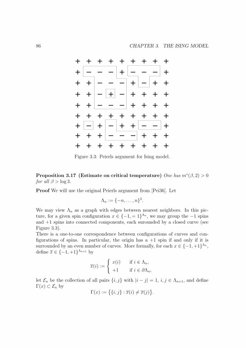
86 CHAPTER 3. THE ISING MODEL
++ + + + + + + +−+ − − + − − − +++ − − − + − + +++ − + − + + + +++ − − − + + + +++ + + + + + + +−+ + − + + − − +++ + − − − + + +++ + + + + + + +
Figure 3.3: Peierls argument for Ising model.
Proposition 3.17 (Estimate on critical temperature) One has m∗(β, 2) > 0for all β > log 3.
Proof We will use the original Peierls argument from [Pei36]. Let
Λn := −n, . . . , n2.
We may view Λn as a graph with edges between nearest neighbors. In this pic-ture, for a given spin configuration x ∈ −1,= 1Λn , we may group the −1 spinsand +1 spins into connected components, each surounded by a closed curve (seeFigure 3.3).There is a one-to-one correspondence between configurations of curves and con-figurations of spins. In particular, the origin has a +1 spin if and only if it issurrounded by an even number of curves. More formally, for each x ∈ −1,+1Λn ,define x ∈ −1,+1Λn+1 by
x(i) :=
x(i) if i ∈ Λn,
+1 if i ∈ ∂Λn,
let En be the collection of all pairs i, j with |i − j| = 1, i, j ∈ Λn+1, and defineΓ(x) ⊂ En by
Γ(x) :=i, j : x(i) 6= x(j)
.

3.6. EXISTENCE OF A PHASE TRANSITION 87
LetGn :=
Γ(x) : x ∈ −1,+1Λn
be the configuration of all ‘configurations of curves’. Then the probability of seeinga certain configuration of curves is given by
ρ(Γ) =1
Ze−β|Γ|,
where |Γ| is the total length of the curves in the configuration Γ and
Z :=∑Γ∈Gn
e−β|Γ|
is a normalization constant. Now let γ ⊂ E be a collection of nearest-neighboredges that form a closed curve (not a configuration of curves but just one singlecurve) surrounding the origin. We can ask what the probability is of seeing a con-figuration of curves in which this this particular curve is present. This probabilityis, of course,
1
Z
∑Γ∈Gn: γ⊂Γ
e−β|Γ|
=
∑Γ: γ⊂Γ e−β|Γ|∑
Γ e−β|Γ|
≤∑
Γ: γ⊂Γ e−β|Γ|∑Γ: γ⊂Γ e−β|Γ| +
∑Γ: γ∩Γ=∅ e−β|Γ|
=
∑Γ: γ⊂Γ e−β|Γ|∑
Γ: γ⊂Γ e−β|Γ| + eβ|γ|∑
Γ: γ⊂Γ e−β|Γ|=
e−β|γ|
e−β|γ| + 1≤ e−β|γ|.
Here we use that for every configuration of curves in which γ is present, thereis another configuration in which γ is completely removed, which is a factor eβ|γ|
more likely than the configuration in which γ is present. Since there are at mostk3k different curves γ of length k surrounding the origin, we find that the expectednumber of curves surrounding the origin can be estimated from above by
∞∑k=4
k3ke−kβ.
By choosing β sufficiently small, we can make this number as close to zero as wewish; in particular, this proves that (uniformly (!) in n)
∫µΛn,β
+ (dx)x(0) > 12
forβ sufficiently large.

88 CHAPTER 3. THE ISING MODEL
Unfortunately, this does not quite give the explicit bound we are after. If β > log 3,then we see that the expected number of curves surrounding the origin is finite(where, again, our estimate is uniform in n), but this is not enough to concludethat
∫µΛn,β
+ (dx)x(0) > 12, hence m∗(β) > 0.
To fix this problem, we use a trick. We fix some m ≤ n and look at the proportionof probabilities ∫
µΛn,β+ (dx)1x(i)=−1 ∀i∈Λm∫µΛn,β
+ (dx)1x(i)=+1 ∀i∈Λm.
We note that the event x(i) = −1 ∀i ∈ Λm occurs if and only if there areno contours inside Λm and there is an odd number of contours surroundig Λm.Likewise, the event x(i) = +1 ∀i ∈ Λm occurs if and only if there are nocontours inside Λm and there is an even number of contours surroundig Λm. Wecan estimate the proportion of the probabilities of these events by estimating theexpected number of contours surrounding Λm, conditional on the event that thereare no contours inside Λm. By the same arguments as above, this expectation canbe estimated by
∞∑k=4m
k3ke−kβ,
which in case β > log 3 can be made arbitrarily small by choosing m sufficientlylarge. Now, letting Λn ↑ ∞ while keeping m fixed, using Proposition 3.11, we seethat the upper invariant measure ν satisfies∫
ν(dx)1x(i)=−1 ∀i∈Λm∫ν(dx)1x(i)=+1 ∀i∈Λm
< 1
for some m. In particular, this shows that ν is not symmetric with respect to asimultaneous flip of all spins, hence ν 6= ν. As we have already seen, this impliesthat m∗(β) > 0.
3.7 Other topics
For the Ising model on d = 2, Onsager has shown [Ons44] that
βc = log(1 +√
2)
and
m∗(β, 2) =(1− sinh(β)−4
)1/8(β ≥ βc),

3.7. OTHER TOPICS 89
wheresinh(β) = 1
2
(eβ − e−β
)is the sinus hyperbolicus. Note that in light of this, the estimate βc ≤ log 3 arisingfrom Proposition 3.17 is not so bad! Onsager’s solution also implies that
m∗(β, 2) ∼ (β − βc)1/8 as β ↓ βc,
which shows that the critical exponent associated with the spontaneous mag-netrization is 1/8 in dimension d = 2. It is supposed that
m∗(β, 3) ∼ (β − βc)0.308 as β ↓ βc,
but there is no mathematical theory to explain this. (There is -nonrigorous- renor-malization group theory that sort of ‘explains’ this and even allows one to calculatethe critical exponent with some precision.) This critical exponent can actually bemeasured and has been experimentally observed for various magnetic systems andgasses near the critical point. Obviously, these physical systems are locally notvery similar to the (nearest-neighbor) Ising model, but it is believed (and up tosome level understood by renormalization group theory) that this critical exponentis universal and shared by a large number of different models.Similar to what we know for the contact process, one can prove that for theIsing model, all spatially homogeneous infinite volume Gibbs measures are convexcombinations of ν and ν. In dimension 2, these are in fact all infinite volume Gibbsmeasures, but, contrary to what we saw for the contact process, in dimensionsd ≥ 3 there exist infinite volume Gibbs measures for the Ising model that are nottranslation invariant.Generalizing from the Ising model, one may look at models where spins can takeq = 2, 3, . . . values, described by Gibbs measures with a Hamiltonian of the form(3.9). These models are called Potts models. An interesting feature of these modelsis that while the spontaneous magnetizationm∗(β) is (supposed to be) a continuousof β for the Ising model, it is known that the same is not always true for Pottsmodels. Ising and Potts models can be studied in a nice uniform framework usingthe random cluster model.

90 CHAPTER 3. THE ISING MODEL

Chapter 4
Voter models
4.1 The basic voter model
The standard, nearest-neighbor voter model on Zd is the Markov process withvalues in 0, 1Z defined by the generator
Gf(x) :=∑i
12d
∑j: |i−j|=1
1x(j)6=x(i)(f(xi)− f(x)
), (4.1)
where xi is defined as in (2.2) and the generator is first defined for functions inCsum(0, 1Zd
) and then by closure for a larger class of functions, as explained inChapter 1.
Note that there is no real parameter in (4.1) in which we could observe a phasetransition, comparable to the infection rate of the contact process or the inversetemperature of the Ising model. The only free parameter is the dimension d.Indeed, we will see that the behavior of the voter model depends on whether d ≤ 2or d > 2, where d = 2 is the ‘critical dimension’.
In the classical interpretation of the voter model, sites represent individuals andthe type Xt(i) of a site represents the political opinion held by individual i at timet. (The model was obviously invented in a country with a two-party system like,for example, the USA.) Then (4.1) says that people behave in a conformist way,i.e., they change their opinion at a rate proportional to the number of neighborsthat hold the other opinion. An equivalent way of describing this is to say thatat times of a rate one Poisson point process, an individual decides to update itsopinion by choosing one of its 2d neigbors at randon and adopting its opinion (withthe result that nothing happens if the newly adopted opinion is the same as the
91
92 CHAPTER 4. VOTER MODELS
original opinion). This description suggests a natural way to write (4.1) in termsof local maps, and hence a graphical representation. For each i, j ∈ Zd, let
mij(x)(k) :=
x(i) if k = j,x(k) otherwise.
(4.2)
Then we may rewrite (4.1) as
Gf(x) :=∑i
12d
∑j: |i−j|=1
(f(mij(x))− f(x)
). (4.3)
In a graphical representation, the local map mij is usually represented by an arrowfrom i to j. In a more serious interpretation, we may interpret the type Xt(i) ofa site at a given time as the genetic type of some organism living at this position.Then (4.3) says that organisms die at rate one and after their deaths are replacedby a descendant of one of their neighbors. Thus, the voter model can be used tomodel neutral evolution where the genetic type of an organism has no influence onits fitness. This is often a useful first step towards more complicated models wherethe fitness of types matters. Also, it is believed that large parts of the DNA ofmost organisms consist of ‘junk’ that has no influence on fitness but may still beinteresting in the study descendancy relations.
4.2 Coalescing ancestries
Imagine that for a given voter model, constructed with a graphical representationas described in the previous section, we want to know the type Xt(i) of a site i atsome time t > 0. Then we may look at the last time σ1 < t when an arrow ends ati and hence the site i possibly changed its type. If σ1 < 0, we are done; otherwise,we know that the organism at i was at time σ1 replaced by a descendant of theorganism at the neighboring site j where the arrow starts, so it suffices to followthis organism back in time till the last time σ2 < σ1 that an arrow ended there.Continuing this process, following arrows backwards whenever we meet one thatends at the site where we currently are, we see that for each (i, t) ∈ Zd × R we
can define a Zd-valued process (ξ(i,t)s )s≥0 such that ξ
(i,t)s is the position where the
(unique) ancestor of (i, t) lived at time t − s. In particular, following ancestorsback till time zero, we find that
Xt(i) = X0(ξ(i,t)t ) (i ∈ Zd, t ≥ 0). (4.4)
It is easy to see (compare Theorem 1.12) that (ξ(i,t)s )s≥0 is a random walk that jumps
with rate one to a uniformly chosen neighboring site. Moreover, two ‘ancestral’
4.3. DUALITY 93
random walks started at two different space-time points (i, t) and (i′, t′) behaveindependently as long as they are apart and coalesce (i.e., go together as one) assoon as they meet.
The coalescing random walks (ξ(i,t)s )s≥0 are often called lines of descent. They are
exactly the ‘paths of influence’ from Chapter 1. In view of this, it is easy to seethat the constant K from (1.23) is zero. Therefore, unlike for the contact processand Ising model, the value of this constant tells us nothing about ergodicity of theprocess. Indeed, since the constant configurations 0 and 1 are traps for the model,the delta measures δ0 and δ1 are always invariant measures so the invariant lawis never unique. In many ways, the voter model in any dimension is a ‘critical’model, i.e., it behaves in many ways similar to other models at their critical point.
Proposition 4.1 (Invariant laws in low dimensions) In dimensions d = 1, 2,all invariant laws of the voter model are convex combinations of the delta measuresδ0 and δ1 on the constant configurations 0 and 1.
Proof The voter model stared in any initial law satisfies
P[Xt(i) = Xt(j)] = P[X0(ξ(i,t)t ) = X0(ξ
(j,t)t )] ≥ P[ξ
(i,t)t = ξ
(j,t)t ]. (4.5)
We observe that(ξ
(i,t)s − ξ
(j,t)s
)s≥0
is a Markov process that everywhere outsidethe origin jumps with rate 2 to a uniformly chosen neighbor and when it reachesthe origin is trapped there. Since one-dimensional nearest-neighbor random walkis recurrent in dimensions d = 1, 2, it follows that the right-hand side of (4.5)tends to zero as t→∞. In particular, this means that any invariant law must beconcentrated on constant configurations. Since, on the other hand, δ0 and δ1 areinvariant laws for the voter model, this proves our claim.
4.3 Duality
Our next aim is to prove that in dimensions d > 2, there are invariant laws of thevoter model that are not convex combinations of δ0 and δ1. A convenient way todo this is to use duality.
We have already met the self-duality of the contact process (Lemma 2.1). Moregenerally, two continuous-time Markov processes X and Y with generators GX
and GY and state spaces S and T are called dual to each other, with respect to aduality function Ψ : S × T → R, if
E[Ψ(X0, Yt)] = E[Ψ(Xt, Y0)] (t ≥ 0), (4.6)
94 CHAPTER 4. VOTER MODELS
whenever X and Y are independent (with arbitrary initial laws). Since we canalways integrate over the initial laws, in order to check (4.6), it suffices to provethe statement for deterministic initial states, i.e., (4.6) is equivalent to
Ey[Ψ(x, Yt)] = Ex[Ψ(Xt, y)] (t ≥ 0, x ∈ S, y ∈ T ), (4.7)
where Ex (resp. Ey) denotes expectation with respect to the law of the process X(resp. Y ) started in X0 = x (resp. Y0 = y). If the state spaces S, T are finite, thena necessary and sufficient condition for (4.6) is that
GXΨ( · , y)(x) = GY Ψ(x, · )(y) (x ∈ S, y ∈ T ). (4.8)
This condition, plus some technical assumptions, is also often sufficient for pro-cesses with infinite state spaces, see e.g. [AS09a]. Note that the self-duality of thecontact process fits in this general scheme, where Ψ(A,B) = 1A∩B 6=∅.
Below, for any x, y ∈ 0, 1Zd, we write |x| :=
∑i x(i) and (xy)(i) := x(i)y(i).
Note that in this notation, the self-duality function of the contact process can berewritten as Ψ(x, y) = 1|xy|6=0. It turns out that the same duality function alsoyields a useful dual for the voter model.
Lemma 4.2 (Coalescent dual of the voter model) Let X be a voter modeland let Y be the Markov process with values in 0, 1Zd
and generator
Gcoalf(y) :=∑i
12d
∑j: |i−j|=1
(f(cij(y))− f(y)
), (4.9)
where
cij(y)(k) :=
0 if k = i,y(i) ∨ y(i) if k = j,y(k) otherwise.
(4.10)
Then
P[|XtY0| 6= 0
]= P
[|X0Yt| 6= 0
](t ≥ 0) (4.11)
whenever X and Y are independent.
Proof It suffices to prove the statement for deterministic initial states X0 = x andY0 = y. Set A := i : y(i) = 1. Then
Ys(i) := 1∃j ∈ A : ξ(j,t)s = i (s ≥ 0) (4.12)

4.3. DUALITY 95
defines a Markov process with generator as in (4.9). It follows that
P[|Xty| 6= 0
]= P[x(ξ
(i,t)t ) = 1 for some i ∈ A] = P
[|X0Yt| 6= 0
](t ≥ 0).
(4.13)
The voter model also has an annihilating dual.
Lemma 4.3 (Annihilating dual of the voter model) Let X be a voter modeland let Y be the Markov process with values in 0, 1Zd
and generator
Gannf(y) :=∑i
12d
∑j: |i−j|=1
(f(aij(y))− f(y)
), (4.14)
where
aij(y)(k) :=
0 if k = i,y(i) + y(j) mod(2) if k = j,y(k) otherwise.
(4.15)
ThenP[|XtY0| is odd
]= P
[|X0Yt| is odd
](t ≥ 0) (4.16)
whenever X and Y are independent and either X0 or Y0 are a.s. finite.
Proof As in the previous proof, set A := i : y(i) = 1. Now
Ys(i) := 1ξ(j,t)s = i for an odd number of j ∈ A (s ≥ 0) (4.17)
defines a Markov process with generator as in (4.14). It follows that
P[|Xty| is odd
]= P[x(ξ
(j,t)t ) = 1 for an odd number of j ∈ A]
= P[|X0Yt| is odd
](t ≥ 0).
(4.18)
Remark We may rewrite (4.11) as
E[0|XtY0|] = E[0|X0Yt|] (t ≥ 0) (4.19)
and (4.16) asE[(−1)|XtY0|] = E[(−1)|X0Yt|] (t ≥ 0). (4.20)
More generally, for many nearest-neighbor interacting particle systems, there existduals with respect to a duality function of the form Ψ(x, y) = η|xy|, where η is areal parameter; see [SL95, SL97, Sud00].

96 CHAPTER 4. VOTER MODELS
4.4 Clustering versus stability
In this section, we study the voter model started in product initial laws. Thus, wewill assume that the (X0(i))i∈Zd are i.i.d. with intensity P[X0(i) = 1] = θ ∈ [0, 1].
Theorem 4.4 (Process started in product law) Let X be a d-dimensionalvoter model started in product law with intensity 0 ≤ θ ≤ 1. Then
P[Xt ∈ · ] =⇒t→∞
νθ, (4.21)
where νθ is an invariant law of the process. If d = 1, 2, then
νθ = (1− θ)δ0 + θδ1. (4.22)
On the other hand, in dimensions d ≥ 3, for 0 < θ < 1 the measures νθ areconcentrated on configurations that are not constant.
In dimensions d = 1, 2, this theorem says that in any finite environment of theorigin, at sufficient large times, we see with high probability locally either theconstant configuration 0 or 1. This implies that in the system, there must be largeregions constant type, called clusters, of a size that grows in time. This behavioris called clustering.
On the other hand, in dimensions d > 2, it can be shown that the measures νθare concentrated on configurations in which the spatial intensity of ones (averagedover large blocks) is θ. This type of behavior is called stable behavior.
Proof of Theorem 4.4 We use duality with coalescing random walks. For eachy ∈ 0, 1Zd
with |y| < ∞, let Y y denote the process with generator as in (4.9).Since |Y y
t | is a nonincreasing function of time, the limit
Ny := limt→∞|Y yt | (4.23)
exists a.s. It follows that
P[|Xty| = 0
]= P
[|X0Y
yt | = 0
]= E
[(1− θ)|Y
yt |]−→t→∞
E[(1− θ)Ny]
. (4.24)
Since the space 0, 1Zdis compact, the laws P[Xt ∈ · ] are automatically tight, so
to prove convergence it suffices that all weak cluster points coincide. Therefore, byLemma 2.2 we see that P[Xt ∈ · ] converges weakly to a probability law νθ whichis uniquely characterized by∫
νθ(dx)1|xy|=0 = E[(1− θ)Ny]
(|y| <∞). (4.25)
4.5. SELECTION AND MUTATION 97
It follows from general arguments (which we now skip) that any long-time limitlaw of an interaction particle system must be an invariant law. In dimensionsd = 1, 2, one has Ny = 1 a.s., which implies that νθ = (1 − θ)δ0 + θδ1. On theother hand, in dimensions d > 2, by the transience of random walk, P[Ny ≥ 2] > 0for all |y| ≥ 2. In fact, it is not hard to see (again we skip the details) that bychoosing a configuration y in which all ones are sufficiently far from each other, foreach n ≥ 1 and ε > 0 we can find y with |y| = n and P[Ny = n] ≥ 1− ε. It followsthat νθ(0) ≤
∫νθ(dx)1|xy|=0 ≤ (1− ε)(1− θ)n + ε. Since n and ε are arbitrary,
if 0 < θ this proves that νθ gives zero probability to the constant configuration 0.By symmetry between the types, if θ < 1, then νθ gives moreover zero probabilityto the constant configuration 1.
Remark Let I denote the set of all invariant laws of the voter model. It is not hardto show that I is a compact, convex subset of the set of all probability measureson 0, 1Zd
. By definition, an element ν ∈ I is called extremal if it cannot bewritten as a nontrivial convex combination of other elements of I, i.e., there donot exist ν1, ν2 ∈ I with ν1 6= ν2 and 0 < p < 1 such that ν = pν1 + (1 − p)ν2.We let Ie denote the set of all extremal elements of I. Then it is known that forvoter models in dimensions d > 2, the measures νθ from (4.21) satisfy νθ ∈ Ie forall θ ∈ [0, 1].
4.5 Selection and mutation
In this section, we consider a generalization of the voter model with generator
Gf(x) := (1 + s)∑i
12d
∑j: |i−j|=1
1x(i)=0, x(j)=1(f(xi)− f(x)
)+∑i
12d
∑j: |i−j|=1
1x(i)=1, x(j)=0(f(xi)− f(x)
)+m
∑i
1x(i)=1(f(xi)− f(x)
),
(4.26)
where s,m ≥ 0 are constants. Note that this says that sites of type 0 adopt thetype 1 at a rate that is 1
2d(1 + s) times the number of neighbors of type 1, but
sites of type 1 adopt the type 0 at a rate that is only 12d
times the number ofneighbors of type 0. Thus, sites of type 1 invade other sites more easily than sitesof type 0, which we can interpret as saying that type 1 has a higher fitness thanthe other type. In addition, sites of type 1 spontaneously change into sites of type0, which models mutation. For example, we can imagine that organisms of type 1own a complex gene that gives them a selective advantage, while organisms of type

98 CHAPTER 4. VOTER MODELS
0 own a damaged, nonfunctional version of the same gene. We ignore mutationsthat spontaneously restore the functionality of a damaged gene. We call s and mthe selection and mutation rates, respectively.
In order to write the generator in (4.26) in terms of local maps, we define
sij(x)(k) :=
1 if k = j, x(i) = 1,x(k) otherwise,
(4.27)
and
pi(x)(k) :=
0 if k = i,x(k) otherwise.
(4.28)
ThenGf(x) =
∑i
12d
∑j: |i−j|=1
(f(mij(x))− f(x)
)+s∑i
12d
∑j: |i−j|=1
(f(sij(x))− f(x)
)+m
∑i
(f(pi(x))− f(x)
).
(4.29)
In the graphical representation, we represent the maps mij as before by an arrow(black, let us say) from i to j. Likewise, we represent the maps sij by red arrowsand the maps pi by a black box. Then black arrows indicate ‘invasion’ events wherethe type at the beginning of the arrow takes over the site at the tip of the arrow.Red arrows are similar, except that they can only be used for the invasion of type1. The black boxes indicate mutations where the type changes to 0 regardless ofwhat it was before.
It turns out that the coalescent dual of the voter model can be generalized to thepresent more general set-up. Let cij be defined as in (4.10) and define local mapsbij by
bij(y)(k) :=
y(i) ∨ y(j) if k = j,y(k) otherwise.
(4.30)
Lemma 4.5 (Branching-coalescent dual) Let X be a voter model with selec-tion and mutation, with generator as in (4.26), and let Y be the Markov processwith values in 0, 1Zd
and generator
Gcoalf(y) :=∑i
12d
∑j: |i−j|=1
(f(cij(y))− f(y)
)+s∑i
12d
∑j: |i−j|=1
(f(bij(y))− f(y)
)+m
∑i
(f(pi(y))− f(y)
).
(4.31)

4.5. SELECTION AND MUTATION 99
ThenP[|XtY0| 6= 0
]= P
[|X0Yt| 6= 0
](t ≥ 0) (4.32)
whenever X and Y are independent.
Proof When we try to follow lines of descent backwards in time as for the usualvoter model, we run into the difficulty that when we encounter the tip of a redarrow, we do not know which site is the true ancestor of our site. We do know,however, that if either the site at the beginning or at the tip of the arrow wasof type 1 before, then the site at the tip will be of type 1 afterwards. Thus, thesolution is to follow the ancestry of both sites backward in time. In this way,we arrive at a dual process consisting of coalescing random walks with additionalbranching events corresponding to the red arrows and deaths corresponding tomutations.
More formally, the proof goes as follows. It suffices to prove the statement fordeterministic initial states X0 = x and Y0 = y. Let us say that a path γ : [s, u]→Zd is open if it satisfies the following rules:
(i) If γt−1 6= γt, then there must be an arrow from (γt−, t) to (γt, t),
(ii) if at time t there is a black arrow from i to j and γt = j, then γt− = i,
(iii) there is no black box at (γt, t) for any t ∈ [s, u].(4.33)
Write (i, s) (j, u) if there is an open path γ : [s, t]→ Zd such that γs− = i andγu = j. Then
Ys(i) := 1∃j s.t. y(j) = 1, (i, t− s) (j, t) (4.34)
defines a Markov process with generator as in (4.31). Thus, (4.32) follows fromthe claim that
|XtY0| 6= 0 if and only if ∃i, j s.t. x(i) = 1, y(j) = 1, (i, 0) (j, t). (4.35)
Indeed, if there is an open path from (i, 0) to (j, t) with x(i) = 1, then it is easyto check that X must be one all along this path, hence in particular Xt(j) = 1.Conversely, if no such path exists, then all ‘potential ancestors’ of the site j attime t can be traced back to sites that were of type 0 at time zero or to mutationevents.
Both the voter model X with selection and mutation and its dual system Y ofrandom walks with coalescence, branching and deaths are very similar in theirbehavior to the contact process. If the mutation rate is too high, then the processesstarted in any finite initial state die out and the delta measure on the constant
100 CHAPTER 4. VOTER MODELS
zero configuration is the only invariant law. If the mutation rate is sufficientlylow (but s > 0), then the processes started in a finite initial state survives withpositive probability and there exists a nontrivial invariant law.
Exercise 4.6 Show that the standard voter model (s = m = 0) started in a finiteinitial state (i.e., |X0| < ∞ a.s.) dies out a.s. (i.e., P[∃t ≥ 0 s.t. Xt = 0] = 1).Hint: martingale convergence.
4.6 Rebellious voter models
In the biological interpretation of the voter model, let us imagine that the types0 and 1 represent two closely related species, which compete for space. We mayimagine that the cause of death of organisms of these species is often competitionwith organisms on neighboring sites, and that organisms experience more com-petition from other organisms of their own species than from those of the otherspecies. The explanation is that the species occupy slightly different ecologicalniches, hence each species has some resources not available to the other species,which reduces competition between different species. To model this effect, wedefine local maps
rijk(y)(l) :=
y(i) if l = j and y(j) = y(k),y(l) otherwise,
(4.36)
which says that if the organisms living at j and k are of the same type, then theorganism at j dies and is replaced by an organism of the type living at i. Then weare interested in the Markov process with generator
Gf(x) :=∑i
12d
∑j: |i−j|=1
(f(mij(x))− f(x)
)+2β
∑i
1(2d)2
∑j: |i−j|=1
∑k: |j−k|=1
(f(rijk(x))− f(x)
),
(4.37)
where 2β ≥ 0 is the extra death rate due to competition with organisms of the samespecies. Up to a trivial rescaling of time and renaming of parameters, this model isa special case of a model introduced in [NP99]. This and similar models have alsobeen studied in [SS08, SV10]. In the traditional interpretation of voter models,the model in (4.37) describes a population where individuals like to disagree withtheir neighbors. In view of this, a one-dimensional model similar to the one in(4.37) has been called the ‘rebellious voter model’ in [SS08].

4.6. REBELLIOUS VOTER MODELS 101
It turns out that the annihilating dual of the voter model can be generalized tothe present more general set-up. To see this, we start by noting that the generatorin (4.37) can be rewritten as
Gf(x) :=∑i
12d
∑j: |i−j|=1
(f(mij(x))− f(x)
)+β∑i
1(2d)2
∑j: |i−j|=1
∑k: |j−k|=1
(f(qijk(x))− f(x)
),
(4.38)
where qijk is the local map
qijk(x)(l) :=
x(i) + x(j) + x(k) mod(2) if l = j,x(l) otherwise,
(4.39)
which combines the effects of rijk and rkji. Let aij be defined as in (4.15) anddefine local maps tijk by
tijk(y)(l) :=
y(l) + y(j) mod(2) if l ∈ i, ky(l) otherwise.
(4.40)
Then we can prove the following result.
Lemma 4.7 (Double branching-annihilating dual) Let X be a ‘rebellious’voter model with generator as in (4.38), and let Y be the Markov process withvalues in 0, 1Zd
and generator
Gdbranf(y) :=∑i
12d
∑j: |i−j|=1
(f(aij(y))− f(y)
)+β∑i
1(2d)2
∑j: |i−j|=1
∑k: |j−k|=1
(f(tijk(y))− f(y)
).
(4.41)
P[|XtY0| is odd
]= P
[|X0Yt| is odd
](t ≥ 0) (4.42)
whenever X and Y are independent and either X0 or Y0 are a.s. finite.
Proof In the graphical representation, we denote the local map qijk by drawingtwo red arrows, starting at i and k, respectively, and both ending at j. Drawing theusual arrows of the voter model dynamics in black, we call a path γ : [s, u] → Zd
open if it satisfies the following rules:
(i) If γt−1 6= γt, then there must be an arrow from (γt−, t) to (γt, t),
(ii) if at time t there is a black arrow from i to j and γt = j, then γt− = i.(4.43)

102 CHAPTER 4. VOTER MODELS
It suffices to prove the statement of the lemma for deterministic initial statesX0 = x and Y0 = y. Set A := i : x(i) = 1 and B := i : y(i) = 1, fix t > 0 anddefine
Ys(i) := 1the number of open paths from (i, t− s) to B × t is odd (4.44)
(s ≥ 0). Then (Ys)s≥0 is a Markov process with generator as in (4.41). It followsthat
|Xty| is odd⇔ the number of open paths from A× 0 to B × t is odd
⇔ |xYt| is odd,
(4.45)
which proves (4.42).
Note that the process Y with generator a in (4.41) describes a system of annihilat-ing random walks, where in addition, with rate β, particles branch by producingtwo new particles on their neighboring sites, which immediately annihilate withany particles that may already be present on these sites. Note that since the num-ber of particles always increases or decreases by a multiple of 2, the process Y isparity preserving, i.e., if |y| is finite and odd (resp. even), then |Yt| is odd (resp.even) at all t ≥ 0. In view of this, the process started with an odd number ofparticles cannot die out. The following facts are known:
• The process X exhibits coexistence, i.e., there is an invariant law concen-trated on configurations that are not constant 0 or 1, if and only if theprocess Y , started with an even number of particles, survives with positiveprobability.
• In dimension d = 1, the process Y started in an even initial state dies outa.s. for any β ≥ 0.
• In dimensions d ≥ 2, and also for non-nearest neighbor processes in dimen-sion d = 1, if β is sufficiently large, then the process Y started in an eveninitial state survives with positive probability.
• In dimensions d ≥ 2, if β is sufficiently small, then the process Y started inan even initial state survives with positive probability.
The last statement, which has been proved in a series of rather long and technicalpapers by Cox and Perkins [CP05, CP06, CMP10], is supposed to be false for non-nearest neighbor processes in dimension d = 1, but here is no proof of this. Also,

4.6. REBELLIOUS VOTER MODELS 103
perhaps surprisingly, it is not known if survival of the even process Y is monotonein the branching rate β, hence in dimensions d ≥ 2 is is also not known if theeven process survives for intermediate values of β (although both statements arebelieved to be true). In general, the study of rebellious voter models and theirduals is made difficult by the fact that they are not monotonous.

104 CHAPTER 4. VOTER MODELS
Bibliography
[AS09a] S.R. Athreya and J.M. Swart. Branching-coalescing particle systems.Erratum. Prob. Theory Relat. Fields. 145(3-4), 639–640, 2009.
[BFM78] R.C. Brower, M.A. Furman and M. Moshe. Critical exponents for thereggeon quantum spin model. Phys. Lett. B 76, 213–219, 1978.
[BG90] C. Bezuidenhout and G. Grimmett. The critical contact process diesout. Ann. Probab. 18(4), 1462–1482, 1990.
[BG91] C. Bezuidenhout and G. Grimmett. Exponential decay for subcriti-cal contact and percolation processes. Ann. Probab. 19(3), 984–1009,1991.
[CMP10] J.T. Cox, M. Merle and E.A. Perkins. Coexistence in a two-dimen-sional Lotka-Volterra model. Electron. J. Probab. 15, paper No. 38,1190–1266, 2010.
[CP05] J.T. Cox and E.A. Perkins. Rescaled Lotka-Volterra models convergeto super-Brownian motion. Ann. Probab. 33(3), 904–947, 2005.
[CP06] J.T. Cox and E.A. Perkins. Survival and coexistence in stochasticspatial Lotka-Volterra models. Probab. Theory Relat. Fields 139(1/2),89–142, 2007.
[Dob71] R.L. Dobrushin. Markov processes with a large number of locallyinteracting components: existence of a limit process and its ergodicity.Problems Inform. Transmission 7, 149–164, 1971.
[Dur88] R. Durrett. Lecture notes on particle systems and percolation. Wads-worth & Brooks/Cole, Pacific Grove, 1988.
[EK86] S.N. Ethier and T.G. Kurtz. Markov Processes: Characterization andConvergence. John Wiley & Sons, New York, 1986.
105
106 BIBLIOGRAPHY
[Gla63] R.J. Glauber. Time-dependent statistics of the Ising model. J. Math.Phys. 4, 294–307, 1963.
[Har74] T.E. Harris. Contact interactions on a lattice. Ann. Probab. 2, 969–988, 1974.
[Har76] T.E. Harris. On a class of set-valued Markov processes. Ann. Probab.4, 175–194, 1976.
[HS05] R. van der Hofstad and A. Sakai. Critical points for spread-out self-avoiding walk, percolation and the contact process above the uppercritical dimensions. Probab. Theory Relat. Fields 132(3), 438–470,2005.
[Isi25] E. Ising. Beitrag zur Theorie des Ferromagnetismus. Zeitschrift furPhysik 31, 253–258, 1925.
[Lig85] T.M. Liggett. Interacting Particle Systems. Springer-Verlag, NewYork, 1985.
[Lig92] T.M. Liggett. The survival of one-dimensional contact processes inrandom environments. Ann. Probab. 20, 696-723, 1992.
[Lig95] T.M. Liggett. Improved upper bounds for the contact process criticalvalue. Ann. Probab. 23, 697–723, 1995.
[Lig99] T.M. Liggett. Stochastic interacting systems: contact, voter and ex-clusion processes. Springer-Verlag, Berlin, 1999.
[LSS97] T.M. Liggett, R.H. Schonmann and A.M. Stacey. Domination byproduct measures. Ann. Probab. 25(1), 71–95, 1997.
[Loe63] M. Loeve. Probability Theory, 3rd edition. Van Nostrand, Princeton,1963.
[NP99] C. Neuhauser and S.W. Pacala. An explicitly spatial version ofthe Lotka-Volterra model with interspecific competition. Ann. Appl.Probab. 9(4): 1226–1259, 1999.
[Ons44] L. Onsager. Crystal statistics, I. A two-dimensional model with anorder-disorder transition. Phys. Rev.65, 117–149, 1944.
[Pei36] R. Peierls. On Ising’s model of ferromagnetism. Proc. CamebridgePhilos. Soc. 36, 477-481, 1936.

BIBLIOGRAPHY 107
[Rem08] D. Remenik. The contact process in a dynamic random environment.Ann. Appl. Probab. 18(6), 2392-2420, 2008.
[SL95] A. Sudbury and P. Lloyd. Quantum operators in classical probabilitytheory. II: The concept of duality in interacting particle systems. Ann.Probab. 23(4), 1816–1830, 1995.
[SL97] A. Sudbury and P. Lloyd. Quantum operators in classical probabilitytheory. IV: Quasi-duality and thinnings of interacting particle systemsAnn. Probab. 25(1), 96–114, 1997.
[SS08] A. Sturm and J.M. Swart. Voter models with heterozygosity selection.Ann. Appl. Probab. 18(1), 59-99, 2008.
[Sud00] A. Sudbury. Dual families of interacting particle systems on graphs.J. Theor. Probab. 13(3), 695–716, 2000.
[SV10] J.M. Swart and K. Vrbensky. Numerical analysis of the rebelliousvoter model. J. Stat. Phys. 140(5), 873–899, 2010.
[ZG88] H. Ziezold and C. Grillenberger. On the critical infection rate of theone-dimensional basic contact process: numerical results. J. Appl.Prob. 25, 1–8, 1988.
Index
B(E), 7JA, 80Ti, 59ZJ , 81Cb(E), 16M(E), 16⇒, 16ηA,st , 40η†A,st , 40 , 39, 45Zd, 37Cfin, 30Csum, 30µPt, 64µf , 64µ ≤ ν, 57µJ , 80η, 56‖ · ‖, 12ρ, 60xi, 38, 69xA, 80B(E), 7C(E), 12Cfin(P(Zd)), 64M1(E), 12P(Zd), 40
algebraof functions, 41
balance
detailed, 77Bernoulli
random variable, 17Boltzmann
constant, 68Borel-σ-field, 7boundary conditions, 75bounded linear operator, 13
cadlag, 15closable
linear operator, 13closed
linear operator, 13closure
of linear operator, 13cluster point, 8clustering, 96coalescence, 93coexistence, 102complete convergence, 66contact process, 37
extinction, 43survival, 43
core of closed operator, 31counting measure, 16coupling, 22critical
exponent, 44infection rate, 43
descent, line of, 93
108

INDEX 109
detailed balance, 77directed percolation, 47distributions
finite dimensional, 15Dobrushin, 4dual
lattice, 48duality, 93
function, 93
energy function, 73equilibrium, 59ergodic
stationary process, 59ergodicity
of interacting particle system, 59extinction
of the contact process, 43
Fellerprocess, 16semigroup, 13
filtration, 15final
of a path, 25finite dimensional distributions, 15flip
spin, 68
generatorFeller semigroup, 13
Gibbs measure, 73graph
of an operator, 13graphical representation, 39
Holder’s inequality, 61Hamiltonian, 73healthy site, 38Hille-Yosida theorem, 14
homogeneous, 59
infected site, 38infection rate, 37initial law, 11, 16integer lattice, 37invasion, 98inverse temperature, 68, 73irreducible, 76Ising model
stochastic, 67Ising model, 67
jump rate, 21
k-dependence, 53kernel
probability, 8
latticeinteger, 37
Liggett, 4line of descent, 93local map, 24
magnetizationspontaneous, 80
marginal, 9Markov
chain, 10semigroup, 20
maximum principle, 13monotone
function, 57process, 78
mutation, 98
nearest neighbour, 38neighbour
nearest, 38neutral evolution, 92

110 INDEX
nonatomic, 19nontrivial
law, 58
open pathin contact process, 39oriented percolation, 48
oriented percolation, 47
partition sum, 73path
in a graphical representation, 25of influence, 26open
in contact process, 39oriented percolation, 48
Peierls argument, 48percolation
directed, 47oriented, 47parameter, 48
Poissoncounting measure, 18point set, 19
Polish space, 7Potts model, 89probability kernel, 8product topology, 24
rate, 21recovery, 38
recovery rate, 38renormalization group, 44reversibility, 76
sample pathscadlag, 15
selection, 98semigroup
Markov, 20
separates pointsclass of functions, 41
shape theorem, 66site, 37Skorohod topology, 15spin, 68spin flip, 68Spitzer, 4spontaneous magnetization, 80stability of voter model, 96starting time
of a path, 25state space, 10stochastic
Ising model, 67stochastic order, 57Stone-Weierstrass theorem, 41supremumnorm, 12survival
of the contact process, 43
temperatureinverse, 68, 73
thinning, 17tightness, 7time-homogeneous, 11transition
kernel, 12probability, 11
transition probabilitycontinuous, 12
translationinvariant, 59operator, 59
type, 91
weak convergence, 16wet
sites, 48