inter-district funding disparities and the limits of ... · pdf file1 | page inter-district...
TRANSCRIPT
1 | P a g e
Inter-district Funding Disparities and the Limits of Pursuing Teacher Equity through
Departmental Regulation
Bruce D. Baker*
Mark Weber
Graduate School of Education
Rutgers University
*Corresponding Author
DRAFT AS OF June 30, 2015

2 | P a g e
State School Finance Inequities and the Limits of Pursuing Teacher Equity through
Departmental Regulation
Abstract
New federal regulations (State Plans to Ensure Equitable Access to Excellent Educators)1
place increased pressure on states and local public school districts to improve their measurement
and reporting of gaps in teacher attributes across schools and the children they serve. The
regulations largely ignore within versus between district distinctions, leaving states to navigate
this terrain. The analyses herein evaluate the extent to which disparities in district and school
level spending measures are associated with disparities in district and school level teacher equity
measures, using data sources and measures cited in the department’s recent policy guidance to
states. Additionally, we ask whether inequality in “access to excellent educators” is greater in
states where school funding inequalities are greater. For larger districts only (>10 schools),
district spending variation explains an important, policy relevant share of school staffing
expenditures in 13 states (NH, NE, ND, VA, ME, NJ, RI, PA, CO, MT, MN, MA, ID). In many
states, including Illinois and New York, there exists a nearly 1:1 relationship between district
spending variation and school site spending variation. In California, Illinois, Louisiana, New
York, Ohio, Pennsylvania and Virginia, district spending is positively associated with
competitive salary differentials, average teacher salaries and numbers of certified staff per 100
pupils. And in each of these states, district poverty rates are negatively associated with
competitive salary differentials, average teacher salaries and numbers of certified staff per 100
pupils. As such, regulatory intervention without more substantive changes to state school finance
systems will likely achieve little.
1 https://www.federalregister.gov/articles/2014/11/10/2014-26456/agency-information-collection-activities-
comment-request-state-plan-to-ensure-equitable-access-to

3 | P a g e
Introduction
New federal regulations (State Plans to Ensure Equitable Access to Excellent Educators)2
place increased pressure on states and local public school districts to improve their measurement
and reporting of gaps in teacher attributes across schools and the children they serve, and
ultimately to mitigate revealed disparities. But, these regulations largely sidestep the extent to
which availability of financial resources might influence the distribution of teachers, pointing a
finger instead at “root causes” such as lack of effective leadership, lack of comprehensive human
capital strategies and otherwise ineffective and inefficient personnel policies.3 Failure to
emphasize the potential role of broader financial disparities as a root cause of inequitable access
to excellent educators, and thus failure to mitigate those disparities, may undermine the
administration’s goals.
Despite a lack of explicit attention to inter-district fiscal disparities as possible root
causes of inequitable access to excellent educators, the administration provides guidance on
measuring teacher equity using existing data sources and measures which either directly or
indirectly involve financial resources. While broadly referencing “inexperienced, unqualified, or
“out-of-field teachers” as a concern,4 the administration’s guidance also cites measures of
2 https://www.federalregister.gov/articles/2014/11/10/2014-26456/agency-information-collection-activities-
comment-request-state-plan-to-ensure-equitable-access-to 3 The recent state policy guidance document notes: “There are a number of possible root causes of equity gaps, including a lack of effective leadership, poor working
conditions, an insufficient supply of well-prepared educators, insufficient development and support for educators, lack of a comprehensive human capital strategy (such as an over-reliance on teachers hired after the school year has started), or insufficient or inequitable policies on teacher or principal salaries and compensation. These are offered as examples of root causes; an SEA should examine its own data carefully to determine the root causes of the equity gaps identified in its State.”
4 For example, ED guidance notes: “At a minimum, an SEA must identify equity gaps based on data from all public elementary and secondary schools
in the State on the rates at which students from low-income families and students of color are taught by inexperienced, unqualified, or out-of-field teachers (see question A-1).”

4 | P a g e
teacher salaries and cumulative school site spending on teacher compensation (as reported in the
recent CRDC collection).5
Coinciding with these new federal regulations are a series of legal challenges in states
including California and New York which claim that state statutes providing due process
protections and defining tenure status for teachers are a primary cause of deficiencies in teacher
qualifications, specifically in districts and schools within districts serving disadvantaged
minority populations (Black, 2016). Implicit in these legal challenges is an assumption that if
statutorily defined tenure status and due process requirements pertaining to teacher dismissal did
not exist, statewide disparities in teacher qualities between higher and lower poverty schools
(under the statutes in question) would be substantially mitigated. Like the federal regulations,
this approach fails entirely to consider that disparities in district financial resources may be
substantial determinants of statewide variations in teacher attributes.
As a basis by which inequality should be determined, the administration places
significant emphasis on variations in concentrations of children in poverty across schools. That
is, resources should be equitably distributed across children by their economic status.6 Just what
“equity” means under the circumstances is left to states to articulate in their proposals, but the
5 Specific measures and data referenced include: “For example, the Department encourages each SEA to carefully review the data submitted by its LEAs for the Civil
Rights Data Collection (CRDC), district level per-pupil expenditures the SEA has submitted to the National Center for Education Statistics (NCES) via the F-33 survey, as well as data that the SEA has submitted to EDFacts regarding classes that are taught by highly qualified teachers (HQT)4 in developing the State Plan, and any other high-quality, recent data that the SEA has that are relevant to the SEA’s State Plan. To assist in this review, the Department sent each SEA its own complete CRDC data file that has been augmented with selected information from other data sources (such as school-level enrollment by race and eligibility for free and reduced-price lunch).”
“Using data from the 2011–2012 school year, each Educator Equity Profile compares a State’s high-poverty and high-minority schools to its low-poverty and low-minority schools, respectively, on the: (1) percentage of teachers in their first year of teaching; (2) percentage of teachers without certification or licensure; (3) percentage of classes taught by teachers who are not HQT; (4) percentage of teachers absent more than 10 days; and (5) average teacher salary (adjusted for regional cost of living differences).”
6 The administration’s guidance defines an “equity gap” as follows: Equity gap: “an equity gap is the difference between the rate at which low-income students or students of color are
taught by excellent educators and the rate at which their peers are taught by excellent educators.”

5 | P a g e
language of the regulations suggests that, at the very least, children in high poverty settings
should not be subjected to fewer total resources or teachers with lesser qualifications – that there
should not be a negative correlation between poverty concentrations and resources.
A significant body of literature explains that in order to strive for more equitable student
outcomes, there in fact should be a positive – progressive – correlation between aggregate
resources allocated and factors such as child poverty concentrations, disability concentrations
and language barriers (Baker and Green, 2014). Baker, Sciarra and Farrie (2009, 2012, 2014)
evaluate the relationship between district poverty concentrations and state and local revenues,
controlling for other cost factors, to rate the relative equity of state school finance systems.
Center for American Progress (2015) proposed several suggestions for federal intervention to
improve inter-district fiscal equity, adopting the equity measures estimated by Baker, Sciarra and
Farrie(2015).7
Others have similarly evaluated funding disparities across schools within districts,
focusing on whether and to what extent school site budgets and related resources are targeted to
schools with higher concentrations of low income children (Ajwad 2006; Baker 2009a, 2012,
2014; Baker, Libby and Wiley, 2015; Chambers, Levin, and Shambaugh 2010; Levin et al.
2013). Baker (2012) simultaneously addresses variations across schools within districts, and
across schools between districts.
The Educator Equity regulations appear to speak to a goal of achieving statewide equity
across schools as the unit of analysis. That is, statewide, across schools, children in high poverty
school setting should not be subjected to less quantity or quality instructional resources than
children in lower poverty schools. The regulations largely ignore within versus between district
distinctions, leaving states to navigate this terrain. Inequities in available resources persist both 7 https://www.americanprogress.org/issues/education/report/2015/05/18/113397/a-fresh-look-at-school-funding/

6 | P a g e
across school districts and across schools within districts, and there exist important relationships
between the two. For example, if one district has far less total funding available than a
neighboring district, it stands to reason that the average resources in the schools in that district
will also be lower, even if there is variation among them within the district.
Organizational features of the public schooling system constrain what varies between
districts versus within districts. Total budgets, for example, are district level concerns. While
state aid formulas fund districts and help determine local tax policy, local property tax (and sales
tax in some cases) revenues are raised by districts. These local budgets support district
compensation structures, teacher contractual agreements including the structure of compensation,
restrictions on assignments, placements and related working conditions that vary across districts
as bargaining units, but not across schools within districts. As such, the competitiveness of a
salary guide is most likely not to vary across schools within any one district. Thus, when
considering root causes of disparities across schools, one must consider what factors can and do
vary only across districts and what others may also vary within them. It would be illogical, for
example, to attribute disparities across schools within districts to contractual constraints in
collective bargaining agreements that vary only between districts. As such, the “root causes” of
within versus between district disparities are likely much different.
Finally, but for a relatively small number of very large city or countywide school
districts, individual districts tend not to have high and low poverty schools, or high and low
minority concentration schools within their boundaries (Reardon and Owens, 2014). As such,
evaluating equity, as framed above, exclusively across schools within districts may provide
extremely limited information – reflecting, for example, only the variations in resources across

7 | P a g e
high to very high poverty schools in one district, and across low to very low poverty schools in
another, but ignoring entirely the disparities between the high and low poverty districts.
The analyses herein evaluate the extent to which disparities in district level spending
measures are associated with disparities in school level teacher equity measures, using data
sources and measures cited in the department’s recent policy guidance to states. Additionally, we
ask whether inequality in “access to excellent educators” is greater in states where school
funding inequalities are greater.
Related Literature
The U.S. Department of Education released a report in 2011, based on a 2008-09 data
collection similar to that used herein, in which the department characterized differences in
spending between higher and lower poverty schools within districts.8 The report was intended to
inform deliberations over comparability regulations in Title I of the Elementary and Secondary
Education Act. Comparability guidance, related to the distribution of Title I funding, focuses
exclusively on comparability of resources across schools within districts. The report found a
significant share of Title I schools within districts – those with relatively higher shares of low
income students – having fewer total resources (total salaries per pupil) than the average for their
district; however, it ignored entirely differences between the average level of resources available
in the districts of those Title I schools compared to surrounding districts. The report also ignored
whether and to what extent these differences might be explained by the distribution of children
with other needs, including children with disabilities.
The Title I comparability study follows a long line of studies of within-district resource
allocation produced mainly from the 1990s onward, including analyses of school site
8 http://www2.ed.gov/rschstat/eval/title-i/school-level-expenditures/school-level-expenditures.pdf
8 | P a g e
expenditures from financial data systems, school site personnel spending specifically, and in
some cases specific characteristics of teachers across schools. Studies conducted in the 1990s
found significant disparities in resources within districts (Burke, 1999, Steifel, Rubenstein &
Berne, 1998). Rubenstein, Schwartz, Stiefel, and Bal Hadj Amor (2007) confirm and expand on
earlier findings regarding the distribution of teachers by their qualifications across schools:
“Using detailed data on school resources and student and school characteristics in New York
City, Cleveland and Columbus, Ohio, we find that schools with higher percentages of poor
pupils often receive more money and have more teachers per pupil, but the teachers tend to be
less educated and less well paid, with a particularly consistent pattern in New York City
schools.”
Houck (2010) found similar patterns in Nashville, and Baker (2012) found similar
patterns in some Texas school districts. Baker (2012) found, for example, that school site
spending is relatively progressively distributed with respect to low income concentrations across
schools in Austin and Houston (and Fort Worth), but less so in Dallas. In Austin, these school
site spending differences translated to higher numbers of staff per pupil, but also higher shares of
inexperienced staff. Austin and Houston schools on average had marginally higher per pupil
spending than schools in surrounding, lower poverty districts, but this was not so for schools in
Dallas, constraining that district’s ability to reshuffle resources.
Ajwad (2006) also used data on Texas school level expenditures for elementary schools
to evaluate whether Texas school districts have targeted greater resources toward schools in
higher poverty neighborhoods. Using fixed effects expenditure functions, Ajwad shows that
Texas school districts, on average, target additional resources toward elementary schools in
higher poverty neighborhoods, using neighborhood resident population characteristics rather than

9 | P a g e
school enrollments. Ajwad finds that on average, the dollar differences in targeted funding are
relatively small, and does not disaggregate findings for specific large districts or their neighbors.
Baker, Libby and Wiley (2015) explore how within jurisdiction equity is affected by the
introduction of independently operated charter schools which induce uneven sorting of students
by their needs, and also introduce potential financial inequalities through more aggressive private
fundraising than is typical among individual district schools. Baker, Libby and Wiley (2015) find
specifically regarding New York City that many charter schools simultaneously serve relatively
low need student populations and raise substantial philanthropy to boost their spending, resulting
in a subset of higher spending, lower need schools and disrupting equity.
Baker and Welner (2009) explain that emphasis in the 1990s and 2000s on within district
resource variations, and interest in federal policy tools like Title I Comparability regulations
became somewhat of a distraction from the persistent between-district inequities of many state’s
education systems. A related body of largely non-peer reviewed, empirically problematic
literature emerged by the late 1990s through mid-2000s asserting that years of litigation and
attention to state school finance systems had largely resolved between district variations, leaving
as the primary source of inequity – local district budgeting and teacher assignment practices
(Baker and Welner, 2009).
Several recent reports have reaffirmed the extent of persistent poverty-related inequalities
across districts within states and have illustrated that during the recession, many of those
disparities worsened (Baker, Sciarra and Farrie, 2009, 2012, 2014; Baker and Corcoran, 2012;
Baker, 2014a, Baker, 2014b). Baker (2014) identifies several districts around the nation where
U.S. Census Bureau poverty rates are substantially higher (more than double) than those of

10 | P a g e
surrounding districts and where per pupil state and local revenue is substantially lower (<90%)
than in surrounding districts.
Teachers are inequitably distributed across districts as well. Findings from over a decade
ago and from more recent years confirm that variations in the attributes and qualifications of
teachers tend to vary as much, if not more, between districts than across schools within them
(Goldhaber, Lavery & Theobald, 2014; Lankdford, Loeb and Wyckoff, 2002). In one of the first
major studies kicking off the modern wave of “teacher equity” analyses, Lankford, Loeb and
Wyckoff evaluated the distribution of teacher attributes across schools and districts in New York
State using statewide administrative data. They found that “lesser-qualified teachers teach poor,
nonwhite students,” and that “Much of these differences are due to differences in average
characteristics of teachers across districts, not within urban districts; but differences among
schools within urban districts are important as well.” (Lankford, Loeb, Wyckoff, 2002, p. 47) In
more recent work, Goldhaber and colleagues explored the distribution of direct measures of
teacher “effect” on student outcomes, along with measures of teacher qualifications, using
administrative data on teachers in the State of Washington (Goldhaber, Lavery & Theobald,
2014). Specifically, Goldhaber and colleagues evaluated “teacher gaps” with respect to school
level concentrations of low income students (those qualifying for free or reduced priced lunch, or
FRL), and minority students. The authors note:
For example, the teacher quality gap for FRL students appears to be driven equally by
teacher sorting across districts and teacher sorting across schools within a district. On the
other hand, the teacher quality gap for URM (underrepresented minority) students
appears to be driven primarily by teacher sorting across districts; i.e., URM students are

11 | P a g e
much more likely to attend a district with a high percentage of novice teachers than non-
URM students.9
Washington State differs from New York State in that 1) there exists far less variation in total
available district resources across the state, reducing the potential for between district variation
(Baker, Sciarra, Farrie, 2015) and 2) districts operate under a statewide salary structure, also
reducing potential for between-district variation which might more severely disadvantage higher
need districts.10 Yet still, between-district variations in teacher characteristics with respect to
low-income concentrations were equal to or greater than within district variations, and between
district disparities with respect to minority concentrations were greater than within district
disparities.
Finally, a substantial body of literature has accumulated over the decades to validate the
conclusion that both teachers’ overall wages and relative wages affect the quality of those who
choose to enter the teaching profession, and whether they stay once they get in. For example,
Murnane and Olson (1989) found that salaries affect the decision to enter teaching and the
duration of the teaching career, while Figlio (1997, 2002) and Ferguson (1991) concluded that
higher salaries are associated with more qualified teachers. Research on the flip side of this issue
– evaluating spending constraints or reductions – reveals the potential harm to teaching quality
that flows from leveling down or reducing spending. For example, Figlio and Rueben (2001)
note that, “Using data from the National Center for Education Statistics we find that tax limits
systematically reduce the average quality of education majors, as well as new public school
teachers in states that have passed these limits.”
9 http://www.cedr.us/papers/working/CEDR%20WP%202014-4.pdf
10 http://www.k12.wa.us/LegisGov/SalaryAllocations.aspx

12 | P a g e
While several studies show that higher salaries relative to labor market norms can draw
higher quality candidates into teaching, the evidence also indicates that relative teacher salaries
across schools and districts may influence the distribution of teaching quality. For example,
Ondrich, Pas and Yinger (2008) “find that teachers in districts with higher salaries relative to
non-teaching salaries in the same county are less likely to leave teaching and that a teacher is less
likely to change districts when he or she teaches in a district near the top of the teacher salary
distribution in that county.” Similarly, and most closely related to the questions addressed herein,
Adamson and Darling-Hammond (2012) in an analysis of the distribution of teacher attributes
across California and New York school districts, found that “increases in teacher salaries are
associated with noticeable decreases in the proportions of teachers who are newly hired,
uncredentialed, or less well educated.” (p. 1)
Conceptual Model
The conceptual model here, illustrated in Figure 1, is simple. The assumption herein,
drawing on the literature cited above, is that financial resource availability is an important driver
of access to teaching resources. The level of funding available to local public school districts
plays a role in determining the level of specific school site spending on teacher related resources
in the aggregate, including the relative competitiveness of teacher compensation and, quite
possibly, resulting teacher qualifications. Further and central to the proposed investigation,
inequities in financial resources across local public school districts may, in part, be a root cause
of inequities in specific school site spending related to teaching, including competitiveness of
salaries and qualifications.

13 | P a g e
Figure 1 – Conceptual Model
Financial Resources Teaching Resources
District Spending School Site Instructional
Spending
Salaries Qualifications
The overall level of funding available in local public school districts determines both the
qualities and quantities of staffing, which is realized in the breadth of course offerings at the
secondary level and in class sizes. Local public school districts may leverage additional
resources to either hire more staff – leading to expanded programs and reduced class sizes – or
pay existing staff higher wages in the interest of recruiting and retaining more qualified staff.
Further, these two choices interact in important ways, as smaller classes and lower total student
loads create more desirable working conditions.
Research Questions
The empirical analyses that follow attempt to address two broad research questions:
1. How much variation in school site aggregate resources is explained by variation in
district resources, among districts at similar poverty concentrations and for schools
serving similar grade ranges and of similar size?
2. To what extent does variation in district level spending influence variation in specific
school site resources including a) total school site staffing expenditure, b) school site
instructional expenditure, c) competitiveness of school site teacher salaries, d)
average teacher salaries, and e) school staffing ratios?
3. Finally, to what extent does inter-district funding progressiveness explain statewide,
inter-school resource progressiveness?

14 | P a g e
Methods
The goal herein is to understand variations in resources across schools within and across
school districts. As such one must identify measures and construct appropriate models in order to
parse the equitable variations from the inequitable ones. Among other factors, when evaluating
resources across schools or districts, statewide or nationally, one must account for variations in
labor costs. A relatively simple method for addressing the purchasing power of the school dollar
is to compare school and district spending among districts and schools sharing the same labor
market. We use the labor market delineations adopted by Taylor and Fowler (2005) for
estimating the Education Comparable Wage Index. Instead of using the index itself, we re-
express both spending and poverty measures (because they similarly depend on invariant income
measures) for all districts and schools relative to (as a ratio to) the average of all districts and
schools sharing the same labor market. Other measures used to explain school level spending
variations include the shares of children with limited English language proficiency and shares of
children classified for special education services under the Individuals with Disabilities in
Education Act (IDEA) (Duncombe and Yinger, 2008). Table 1 identifies the various data sources
and measures used herein.
Grade range disparities in resources and disparities due to school total enrollment size
complicate equity analyses. In population dense metropolitan areas, the choice to subsidize small
schools at a higher rate is just that, a policy choice, and one that creates unnecessary inequity.
Nonetheless, we do choose to compare, herein, smaller schools to smaller schools and larger
ones to larger ones using school size dummy variables. To capture spending differences
associated with grade ranges served by schools, we use measures of the percent of students in a
school falling in certain grade ranges. Again, it is a policy choice, not necessarily an

15 | P a g e
uncontrollable cost that more or fewer funds are allocated to schools serving certain grade
ranges. But for simplicity herein, we choose to compare schools serving similar grade ranges and
leave for another day any critique of inequities induced by the choice to operate small schools
and organize schools in certain ways by grade ranges.

16 | P a g e
Table 1. Data and Measures
Measure Type Measure (Specification)
Data Source Notes / Construction Sample/Link
District Geographic Location
Labor Market Education Comparable Wage Index [1]
Based on Census Core Based Statistical Areas
District Universe
District Resource Current Spending per Pupil (ratio to labor market average)
Census Fiscal Survey [2] PPCSTOT District Universe
District Poverty Child Poverty Rate (ratio to labor market average)
Census Small Area Income and Poverty Estimates [3]
District Universe
School Resource Total Salaries per Pupil (ratio to labor market average)
“Equitable Access to Excellent Educators” [4]
TOT_SALARIES/ member11
School Universe
Instructional Salaries per Pupil (ratio to labor market average)
“Equitable Access to Excellent Educators” [4]
INST_SALARIES / member11
School Universe
Average Teacher Salary (ratio to labor market average)
“Equitable Access to Excellent Educators” [4]
AVG_TEACH_SALARY
School Universe
Certified Staff per 100 Pupils (ratio to labor market average)
“Equitable Access to Excellent Educators” [4]
FTE_CERT/ (member11/100)
School Universe
Salary Competitiveness Index
Based on Schools and Staffing Survey data [5]
Regression based (see methods below)
School Sample
School Covariates Enrollment Grade Distribution (%pk-5, %6-8, % 9-12)
NCES Common Core, Public School Universe [6]
School Universe
% IDEA Classified Special Education
“Equitable Access to Excellent Educators” [4]
( M_DIS_IDEA_7_ENROL + F_DIS_IDEA_7_ENROL)/( M_TOT_7_ENROL + F_TOT_7_ENROL)
School Universe
% Qualified for Free Lunch
Based on Schools and Staffing Survey data [5]
frelch/member School Universe
% ELL “Equitable Access to Excellent Educators” [4]
( M_LEP_7_ENROL + F_LEP_7_ENROL)/( M_TOT_7_ENROL + F_TOT_7_ENROL)
School Universe
[1] Updated version of NCES Education Comparable Wage Index, provided by Lori Taylor, Texas A&M University. http://bush.tamu.edu/research/faculty/taylor_CWI/ Documentation at: http://nces.ed.gov/pubsearch/pubsinfo.asp?pubid=2006321 [2] U.S. Census Fiscal Survey of Local Governments, Elementary and Secondary Education Finances: http://www.census.gov/govs/school/ [3] U.S. Census Bureau Small Area Income and Poverty Estimates. http://www.census.gov/did/www/saipe/data/schools/data/index.html [4] “Equitable Access to Excellent Educators” http://www2.ed.gov/programs/titleiparta/resources.html [5] Schools and Staffing Survey, National Center for Education Statistics, Restricted Use Data (License #XXXXX) http://nces.ed.gov/pubsearch/pubsinfo.asp?pubid=2014356 [6] Common Core of Data, Public School Universe, National Center for Education Statistics. http://nces.ed.gov/ccd/pubschuniv.asp
Like the previous Title I Comparability study conducted by the Department of Education,
our dependent measures of interest include the two major, aggregate school resource measures
collected in 2011-12: Total Salaries per Pupil and Instructional Salaries per Pupil. We also

17 | P a g e
explore two teacher compensation related measures and one teacher quantity measure. Relying
on the equity profiles data, we include a measure of “average teacher salary” and a measure of
the number of certified staff per 100 pupils. Our final measure is derived only for a sample of
schools in each state, based on modeled data from the NCES Schools and Staffing Survey. In all
cases, our school resource measures are expressed relative to all other schools in the same labor
market.
To construct the Salary Competitiveness Index, we use data from the National Center for
Education Statistics Schools and Staffing Survey (2011-12), which sampled approximately
50,000 teachers and is intended to achieve state representative samples. Our goal is to estimate
an index of the extent to which teacher salaries vary, from one school or district to the next, for
teachers of similar qualifications, under similar contracts and with similar jobs roles. We
estimate a regression model (ordinary least squares) of teachers’ salaries from teaching, as a
function of their job classification, contract days per year, degree level and years of experience,
with dummy variables for each labor market (within state) across the country.
Salary =f(Labor Market Fixed Effect, Job Classification, Contract Days, Degree Level,
Years of Experience)
This allows us to then predict each teacher’s salary, given their job and credentials, for each
labor market – or the expected salary for a teacher like them, in their labor market. The ratio of
each teacher’s actual salary to the expected salary is the competitiveness index for that teacher’s
salary.
Competitiveness Index = Actual Teacher Salary/Predicted Teacher Salary

18 | P a g e
The average salary competitiveness index for all teachers in the same school or district is then
the average salary competitiveness of teacher salaries under the negotiated agreement for any
given school or district.
Upon constructing our various school level resource indices, the next step is to estimate
both state by state and national models of the sensitivity of school site resource measures to
district level spending measures. Again, all resource and spending measures are relative to labor
market averages.
Exploring School Site Spending Variance Within and Between Districts
Our first goal is to understand the variance in total school site resources explained by
district characteristics and populations served, while controlling for school grade ranges served
and school size. This analysis involves only districts with at least 10 schools – those with
sufficient numbers of schools to display within district variation. Many school districts around
the country have no more than one or a few schools per grade level; in such cases, between-
district variations are between school variations. This fact is often lost in conversations about
“fixing” inequity by focusing on within district variation. Focusing on within-district, between-
school variation is of little value for those districts not large enough to have multiple schools
serving any particular grade level or range.
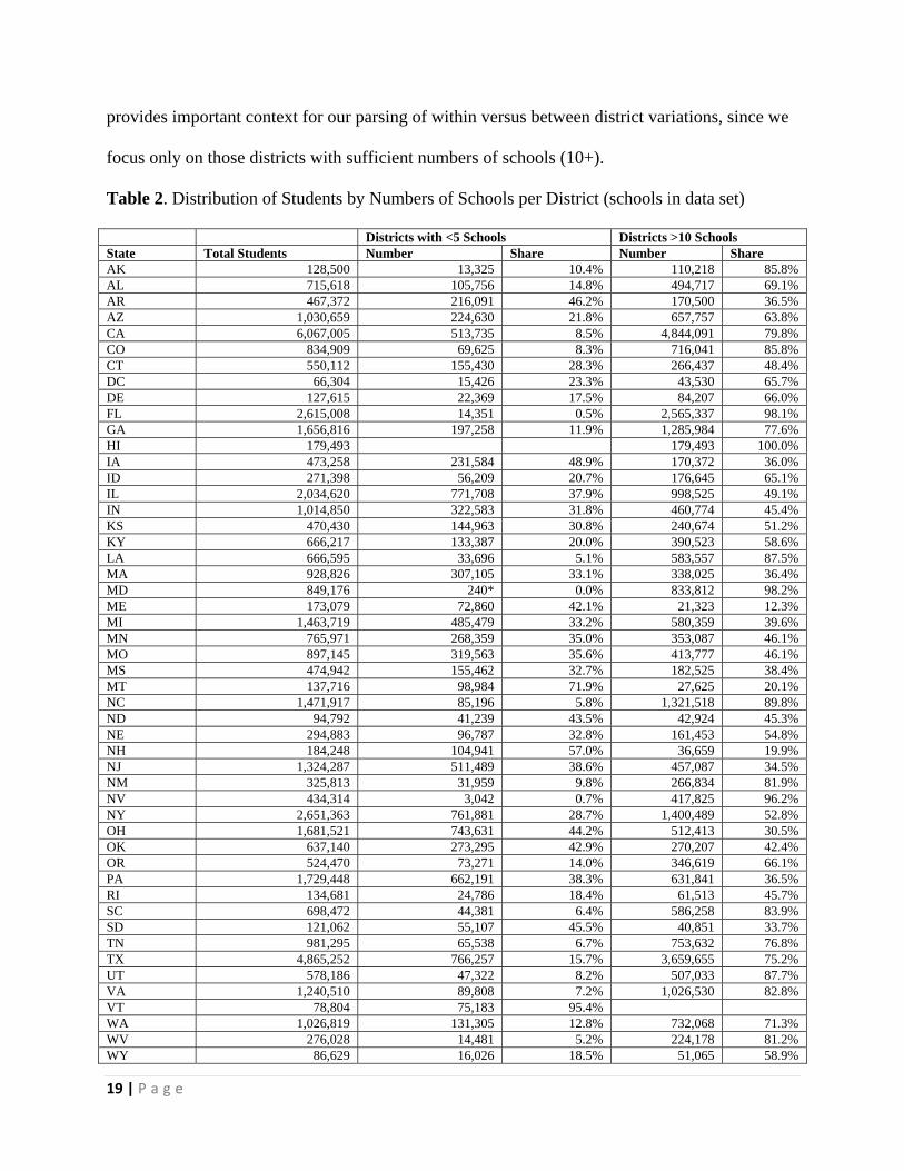
For example, Table 2 shows that 21 states have less than half of students attending
districts with 10 or more schools. Vermont has none. 15 states have more than 1/3 of their
students attending districts with fewer than 5 schools (meaning likely fewer than 3 at any grade
level, 3 elementary, 1 middle, 1 secondary, or single high school regional districts). Table 2
19 | P a g e
provides important context for our parsing of within versus between district variations, since we
focus only on those districts with sufficient numbers of schools (10+).
Table 2. Distribution of Students by Numbers of Schools per District (schools in data set)
Districts with <5 Schools Districts >10 Schools State Total Students Number Share Number Share AK 128,500 13,325 10.4% 110,218 85.8% AL 715,618 105,756 14.8% 494,717 69.1% AR 467,372 216,091 46.2% 170,500 36.5% AZ 1,030,659 224,630 21.8% 657,757 63.8% CA 6,067,005 513,735 8.5% 4,844,091 79.8% CO 834,909 69,625 8.3% 716,041 85.8% CT 550,112 155,430 28.3% 266,437 48.4% DC 66,304 15,426 23.3% 43,530 65.7% DE 127,615 22,369 17.5% 84,207 66.0% FL 2,615,008 14,351 0.5% 2,565,337 98.1% GA 1,656,816 197,258 11.9% 1,285,984 77.6% HI 179,493 179,493 100.0% IA 473,258 231,584 48.9% 170,372 36.0% ID 271,398 56,209 20.7% 176,645 65.1% IL 2,034,620 771,708 37.9% 998,525 49.1% IN 1,014,850 322,583 31.8% 460,774 45.4% KS 470,430 144,963 30.8% 240,674 51.2% KY 666,217 133,387 20.0% 390,523 58.6% LA 666,595 33,696 5.1% 583,557 87.5% MA 928,826 307,105 33.1% 338,025 36.4% MD 849,176 240* 0.0% 833,812 98.2% ME 173,079 72,860 42.1% 21,323 12.3% MI 1,463,719 485,479 33.2% 580,359 39.6% MN 765,971 268,359 35.0% 353,087 46.1% MO 897,145 319,563 35.6% 413,777 46.1% MS 474,942 155,462 32.7% 182,525 38.4% MT 137,716 98,984 71.9% 27,625 20.1% NC 1,471,917 85,196 5.8% 1,321,518 89.8% ND 94,792 41,239 43.5% 42,924 45.3% NE 294,883 96,787 32.8% 161,453 54.8% NH 184,248 104,941 57.0% 36,659 19.9% NJ 1,324,287 511,489 38.6% 457,087 34.5% NM 325,813 31,959 9.8% 266,834 81.9% NV 434,314 3,042 0.7% 417,825 96.2% NY 2,651,363 761,881 28.7% 1,400,489 52.8% OH 1,681,521 743,631 44.2% 512,413 30.5% OK 637,140 273,295 42.9% 270,207 42.4% OR 524,470 73,271 14.0% 346,619 66.1% PA 1,729,448 662,191 38.3% 631,841 36.5% RI 134,681 24,786 18.4% 61,513 45.7% SC 698,472 44,381 6.4% 586,258 83.9% SD 121,062 55,107 45.5% 40,851 33.7% TN 981,295 65,538 6.7% 753,632 76.8% TX 4,865,252 766,257 15.7% 3,659,655 75.2% UT 578,186 47,322 8.2% 507,033 87.7% VA 1,240,510 89,808 7.2% 1,026,530 82.8% VT 78,804 75,183 95.4% WA 1,026,819 131,305 12.8% 732,068 71.3% WV 276,028 14,481 5.2% 224,178 81.2% WY 86,629 16,026 18.5% 51,065 58.9%

20 | P a g e
*SEED School listed as independent of district governance
Our baseline model for each state characterizes the variance explained, across all schools
statewide, by school grade ranges served and school size alone. The intent here is to provide
baseline information regarding the variance in total salaries per pupil among schools serving
similar grade range distributions of similar student population size. Subsequent models can then
be compared against these baseline figures.
Total Salaries (ctr) = f(Grade Ranges Served, Student Population Size)
Next, we evaluate the extent that inter-district variations in current spending per pupil explain
additional variance in school site total salaries per pupil.
Total Salaries (ctr) = f(District Spending(ctr), Grade Ranges Served, Size)
Next, we replace the district spending measure with a district fixed effect (series of district
dummy variables) to explain all cross-district variations in school site spending associated with
district characteristics, including spending as well as unobserved differences between districts.
Total Salaries (ctr) = f (District Fixed Effect, Grade Ranges Served, Size)
To the extent that the district fixed effects models explain more variance in school site resources
than did the previous model, unobserved district characteristics are explaining differences in
school site spending, beyond that explained by district spending. Left behind in the residuals of
this model are between-school, within-district variations in school site spending. Comparisons
between the current spending and district fixed effects model provide insights into the extent that
these unobserved district characteristics influence school site spending.
We conclude this analysis by determining the extent that remaining within-district
disparities in total salary resources are explained by differences in student characteristics,

21 | P a g e
specifically low income concentrations, children with limited English language proficiency and
children with disabilities.
Total Salaries (ctr) = f (District Fixed Effect, School Needs, Grade Ranges Served, School
Size)
At this point, the residuals of the OLS regression include variations in school site resources that
are not explained by district characteristics, and not explained by differences in student needs
across schools. Notably, in most states in this analysis the only student need factor positively
associated with school site staffing expenditure is the percent of children with disabilities, but the
magnitude of this effect varies widely across states. Comparing variance explained between this
and the previous model reveals the extent to which within district spending variation is sensitive
to school level differences in student needs.
Estimating Sensitivity of School Resources to District Spending & Poverty
The next analysis explores the sensitivity of various school level resources to variations
in district level spending and district level rates of children from families in poverty. We estimate
models both state by state and nationally, with state fixed effect. Here, using all districts and
schools, our intent is to evaluate the extent to which school resources – including total salary
expenditures, instructional salary expenditures, competitiveness of salaries, average salaries and
staffing ratios – vary as a function of differences in district spending and district poverty rates:
School Resource(ctr) = f(District Spending(ctr), Poverty(ctr), Grade Ranges Served, School
Size, State)

22 | P a g e
Where each school resource measure is expressed relative to labor market averages, as are
district spending and poverty rates. Again, grade ranges served are expressed as the percentages
of students in grades pk-5 and grades 6-8. School size is expressed with two “small school”
dummy variables. As noted above, we first run state by state models and then run a nationwide
model with state fixed effects.
Estimating within State Fairness Indices
Our final analysis involves constructing “fairness” indices of school site resources with
respect to concentrations of low income children, and relating those school site fairness indices
to inter-district fairness indices. Fairness indices compare the resources available in a high
poverty district or school to the resources available in a low poverty school or district in the same
labor market. Fairness indices are expressed at the state level, and generated via regression
models. The first step is to estimate the following model for each resource measure.
Resource = f(State x Income Status, Grade Ranges Served, School Size)
Where, for each of our school level resource measures, we use school level concentrations of
children qualified for free lunch (<130% income threshold for poverty) as our measure of income
status, expressed for each school as a ratio to the labor market average. As with our resource
measures, this puts our poverty measures and thus poverty variation on a common scale across
states and labor markets. The underlying unit – the dollar – varies in value from one state or
labor market to the next, affecting the value of the school spending input, or the value of family
income similarly (Baker, Taylor, Levin, Chambers & Blankenship, 2013). For our district
spending per pupil, we use district level Census poverty rates as our measure of income status.

23 | P a g e
The second step is to generate predicted values for the resource measures at ends of the
poverty/income spectrum. Here, we generate predicted values for each resource measure at 0%
low income and at twice the labor market average. Our fairness ratio is then the ratio of resources
available at twice the labor market average low income concentration to 0% low income. We
then evaluate the correlations between district level fairness in the distribution of current
spending per pupil (interdistrict spending fairness), and our fairness indices for school level
resource measures. That is, we ask: to what extent is fairness of resources across schools
statewide correlated with fairness of district spending statewide?
Findings
This section begins with a decomposition of the variation in school site total staffing
expenditures per pupil. Next, we explore the sensitivity of several school site resource indicators
to variations in inter-district spending, both for each state and across all states. Finally, we
evaluate whether the overall “fairness” of distribution of school site resources is associated with
the overall “fairness” of distribution of district spending across states.
Explaining Statewide Variance in School Site Resources
Table 3 summarizes the variance in school site total salaries per pupil, explained first as a
function of school grade range and size alone, then including district spending per pupil, then
adding a district fixed effect, and finally including student population characteristics. Recall that
this analysis includes only those districts with at least 10 schools. Residual standard deviations
indicate the extent of variation left behind in our residuals, where the dependent measure was
expressed as a ratio to labor market averages such that .5 would indicate total salaries per pupil at
24 | P a g e
50% of labor market average, and 1.5 would indicate total salaries per pupil at 50% above labor
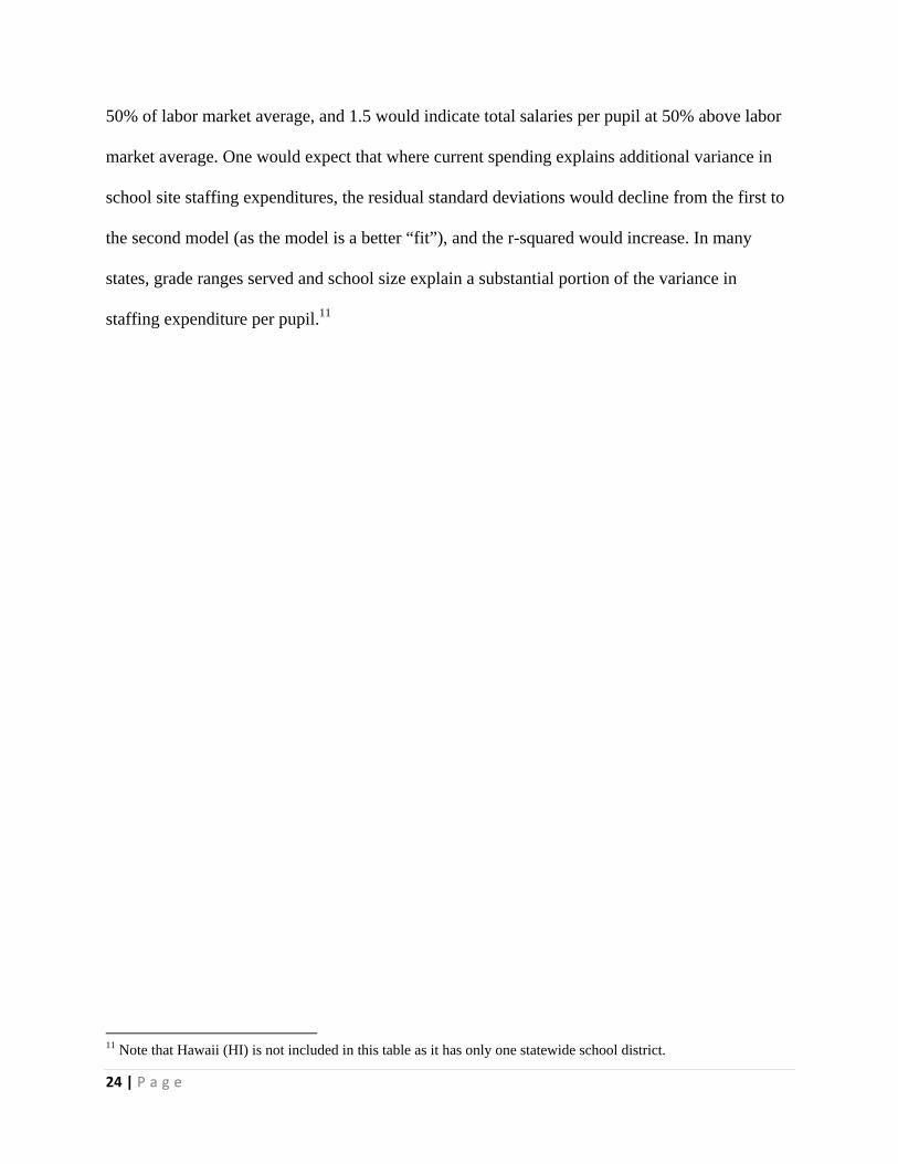
market average. One would expect that where current spending explains additional variance in
school site staffing expenditures, the residual standard deviations would decline from the first to
the second model (as the model is a better “fit”), and the r-squared would increase. In many
states, grade ranges served and school size explain a substantial portion of the variance in
staffing expenditure per pupil.11
11 Note that Hawaii (HI) is not included in this table as it has only one statewide school district.

25 | P a g e
Table 3. Decomposition of Variance in Total Salaries Per Pupil and Variance Explained by District Factors Includes only districts with greater than 10 schools
Conditioned on Grade Level
& School Size Only [1] Conditioned on
District Spending [2]
Conditioned on District Fixed Effect
[3]
Conditioned on District Fixed Effect & Student Needs [4]
State Residual SD R-squared Residual
SD R-
squared Residual
SD R-
squared Residual
SD R-
squared AK 0.265 38.3% 0.265 38.2% 0.253 47.8% 0.246 50.7% AL 0.217 33.4% 0.207 37.4% 0.171 51.3% 0.167 59.6% AR 0.200 39.0% 0.189 41.6% 0.155 60.2% 0.145 64.1% AZ 0.285 17.6% 0.288 17.7% 0.242 30.8% 0.229 35.3% CA 0.343 25.7% 0.339 32.0% 0.293 44.0% 0.293 44.1% CO 0.357 16.5% 0.323 27.4% 0.314 32.9% 0.312 36.3% CT 0.323 22.5% 0.312 23.8% 0.225 53.9% 0.222 54.9% DE 0.284 45.7% 0.282 46.4% 0.215 66.2% 0.115 91.3% FL 0.260 7.7% 0.260 7.8% 0.262 9.3% 0.243 23.4% GA 0.179 28.1% 0.171 32.3% 0.161 38.3% 0.157 41.7% IA 0.280 11.9% 0.249 24.0% 0.217 33.4% 0.181 64.6% ID 0.293 41.4% 0.200 57.6% 0.194 60.2% 0.188 63.6% IL 0.304 27.8% 0.283 31.5% 0.252 42.4% 0.234 52.0% IN 0.192 23.7% 0.185 25.9% 0.160 35.0% 0.159 34.9% KS 0.217 14.6% 0.217 14.8% 0.188 29.9% 0.181 37.4% KY 0.292 38.3% 0.288 40.7% 0.288 46.9% 0.281 50.6% LA 0.283 37.9% 0.279 38.4% 0.260 43.7% 0.244 51.2% MA 0.297 43.8% 0.257 54.1% 0.222 61.5% 0.188 72.4% MD 0.260 8.2% 0.262 8.7% 0.207 25.4% 0.210 30.1% ME 0.157 13.8% 0.137 48.1% 0.124 47.7% 0.125 61.8% MI 0.312 16.7% 0.300 19.5% 0.266 26.9% 0.239 51.0% MN 0.361 15.2% 0.393 31.8% 0.352 43.7% 0.341 45.1% MO 0.266 20.1% 0.262 20.4% 0.194 43.0% 0.196 43.0% MS 0.195 26.6% 0.194 27.1% 0.187 35.2% 0.173 54.3% MT 0.162 15.2% 0.149 32.0% 0.100 69.7% 0.097 70.2% NC 0.262 32.3% 0.262 32.4% 0.245 39.7% 0.236 46.8% ND 0.276 6.1% 0.254 15.9% 0.254 24.7% 0.254 23.4% NE 0.194 6.5% 0.178 18.5% 0.146 43.0% 0.132 50.9% NH 0.153 5.0% 0.119 33.9% 0.108 33.4% 0.093 42.2% NJ 0.271 19.8% 0.236 37.4% 0.199 50.0% 0.192 51.8% NM 0.250 22.3% 0.249 25.9% 0.220 34.0% 0.225 37.1% NV 0.247 38.0% 0.253 40.8% 0.264 45.0% 0.266 44.9% NY 0.298 12.2% 0.296 12.6% 0.267 23.9% 0.182 63.6% OH 0.274 21.1% 0.253 27.5% 0.204 39.1% 0.197 44.8% OK 0.279 31.9% 0.276 33.3% 0.194 61.8% 0.182 65.4% OR 0.199 12.2% 0.183 20.1% 0.168 32.3% 0.154 39.9% PA 0.239 17.8% 0.214 27.8% 0.156 50.2% 0.156 50.5% RI 0.265 21.4% 0.236 34.8% 0.217 44.2% 0.209 45.4% SC 0.205 16.5% 0.198 24.6% 0.178 33.6% 0.166 52.4% SD 0.189 21.6% 0.209 23.5% 0.202 22.1% 0.199 41.0% TN 0.247 29.9% 0.246 29.9% 0.249 34.0% 0.243 41.1% TX 0.246 34.3% 0.243 34.5% 0.211 41.4% 0.209 42.1% UT 0.489 24.9% 0.488 24.8% 0.474 29.2% 0.472 29.1% VA 0.274 5.5% 0.255 15.4% 0.180 52.8% 0.170 56.5% WA 0.228 7.9% 0.217 11.8% 0.184 21.7% 0.181 23.4% WV 0.270 15.4% 0.266 16.4% 0.223 33.1% 0.221 36.3% WY 0.219 47.1% 0.232 47.4% 0.234 49.2% 0.254 49.6% [1] Where school site total salaries per pupil are expressed as a function of a) school size, and b) school grade ranges served. [2] Where school site total salaries per pupil are expressed as a function of a) district current spending per pupil, b) school size, c) school
grade ranges served. Both district current spending and school total salaries per pupil are expressed as a ratio to the average for all districts or schools sharing the same labor market.

26 | P a g e
[3] Where school site total salaries per pupil are expressed as a function of a) district fixed effect [dummy variable], b) school size, c) school grade ranges served. Both district current spending and school total salaries per pupil are expressed as a ratio to the average for all districts or schools sharing the same labor market.
[4] with school level student need factors added to the district fixed effect model, including a) labor market centered % qualified for free lunch, b) percent on special education IEP under IDEA, and c) percent ELL.
The following scatterplots reveal the substantial changes that occur when only district
spending is included in the model, then district fixed effect is added, followed by school level
student needs. For states in the lower left corner of Figure 2, relatively little variance in school
site spending is explained by school structural characteristics (size and grade levels) and/or
district spending. District spending variation adds little to the explanation of school site spending
variation in Florida, for example. By contrast, including district spending in the model
appreciably increases its ability to explain the variations in school site spending in New
Hampshire, Nebraska, North Dakota and Virginia. Toward the mid-range of the figure, district
spending variation appears to explain a substantial additional amount of variation in school site
resources in Maine, New Jersey, Rhode Island, Pennsylvania, Colorado, Montana and
Minnesota. District spending variation also explains noticeable additional variation in
Massachusetts and Idaho, two states where school structural characteristics already explained
much of the variation in total salaries per pupil. For these states in particular, inter-district
spending disparities appear to substantively affect statewide inter-school spending disparities,
thus limiting the efficacy of within-district only equity solutions.

27 | P a g e
Figure 2. Additional Variance Explained by District Spending
Figure 3 reveals the additional variance explained by replacing the district spending
measure with a district fixed effect. As noted previously, the district fixed effect model evaluates
the extent to which any district characteristics explain statewide, inter-school disparities. This
might include some districts, on average, allocating significantly more or less to school site
spending. These differences may occur either by choice, or as a function of structural constraints
that vary across districts, such as shares of children with disabilities, or shares of funding
received from federal or other restricted revenue sources (see Baker, 2003). Still, very little
statewide variation in inter-school spending is explained in Florida. Whatever the unobserved
characteristics, district fixed effects explain substantial additional variation in school site
spending in Virginia, Connecticut, Montana, Nebraska, Missouri and Pennsylvania. That said, it
is difficult to know at this stage what share of that variation is within versus outside the control
of local school officials.
AKAL
AR
AZ
CA
CO
CT
DE
FL
GA
HI
IA
ID
IL
IN
KS
KYLA
MA
MD
ME
MI
MN
MO
MS
MT NC
ND
NE
NH
NJ
NM
NV
NY
OH
OK
OR
PA
RI
SCSD
TN
TX
UT
VA
WA
WV
WY
.1.2
.3.4
.5.6
Var
ianc
e E
xpla
ined
- D
istr
ict S
pend
ing
0 .1 .2 .3 .4 .5Variance Explained - Size & Grade Only

28 | P a g e
Figure 3. Additional Variance Explained by District Fixed Effect
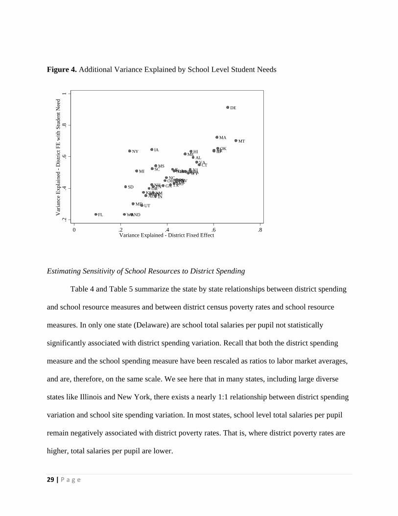
Figure 4 shows the effect if school level student population characteristics are included in
the model. We include this model to show the extent that the remaining within district variations
in staffing expenditure may be explained by school level cost factors, including the distribution
of special education programs and children. Like school size and grade configurations,
distributions of special education programs and children may be influenced by district policy
choices, though the aggregate numbers of children to be served districtwide may not be. Here we
see, for example, that including student characteristics changes substantially the amount of
variation in school site spending explained in New York State, where one third of the student
population attends a single district – New York City – but a district in which special education
population shares alone explains substantial variation in spending across schools (see Baker,
Libby & Wiley, 2015).
AKAL
AR
AZ
CA
CO
CT
DE
FL
GA
HI
IA
ID
IL
IN
KS
KYLA
MA
MD
ME
MI
MNMO
MS
MT
NC
ND
NE
NH
NJ
NM
NV
NY
OH
OK
OR
PA
RI
SC
SD
TN
TX
UT
VA
WA
WV
WY
0.2
.4.6
.8V
aria
nce
Exp
lain
ed -
Dis
tric
t Fix
ed E
ffec
t
.1 .2 .3 .4 .5 .6Variance Explained - District Spending
29 | P a g e
Figure 4. Additional Variance Explained by School Level Student Needs
Estimating Sensitivity of School Resources to District Spending
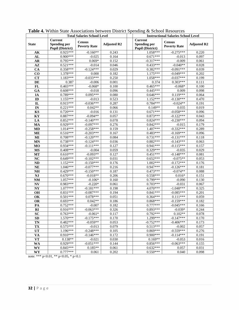
Table 4 and Table 5 summarize the state by state relationships between district spending
and school resource measures and between district census poverty rates and school resource
measures. In only one state (Delaware) are school total salaries per pupil not statistically
significantly associated with district spending variation. Recall that both the district spending
measure and the school spending measure have been rescaled as ratios to labor market averages,
and are, therefore, on the same scale. We see here that in many states, including large diverse
states like Illinois and New York, there exists a nearly 1:1 relationship between district spending
variation and school site spending variation. In most states, school level total salaries per pupil
remain negatively associated with district poverty rates. That is, where district poverty rates are
higher, total salaries per pupil are lower.
AK
AL
AR
AZ
CA
CO
CT
DE
FL
GA
HIIA ID
IL
INKS
KYLA
MA
MD
ME
MI
MNMO
MS
MT
NC
ND
NE
NH
NJ
NM
NV
NY
OH
OK
OR
PA
RI
SC
SD TN TX
UT
VA
WA
WV
WY
.2.4
.6.8
1V
aria
nce
Exp
lain
ed -
Dis
tric
t FE
with
Stu
dent
Nee
d
0 .2 .4 .6 .8Variance Explained - District Fixed Effect
30 | P a g e
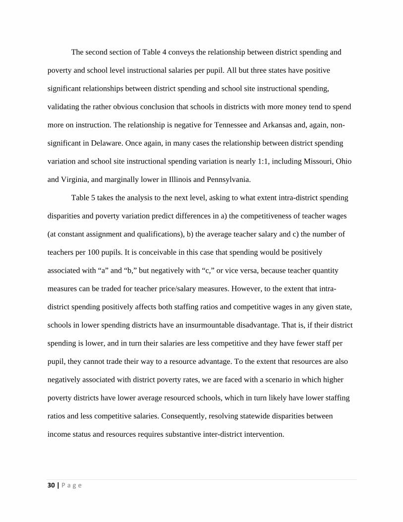
The second section of Table 4 conveys the relationship between district spending and
poverty and school level instructional salaries per pupil. All but three states have positive
significant relationships between district spending and school site instructional spending,
validating the rather obvious conclusion that schools in districts with more money tend to spend
more on instruction. The relationship is negative for Tennessee and Arkansas and, again, non-
significant in Delaware. Once again, in many cases the relationship between district spending
variation and school site instructional spending variation is nearly 1:1, including Missouri, Ohio
and Virginia, and marginally lower in Illinois and Pennsylvania.
Table 5 takes the analysis to the next level, asking to what extent intra-district spending
disparities and poverty variation predict differences in a) the competitiveness of teacher wages
(at constant assignment and qualifications), b) the average teacher salary and c) the number of
teachers per 100 pupils. It is conceivable in this case that spending would be positively
associated with “a” and “b,” but negatively with “c,” or vice versa, because teacher quantity
measures can be traded for teacher price/salary measures. However, to the extent that intra-
district spending positively affects both staffing ratios and competitive wages in any given state,
schools in lower spending districts have an insurmountable disadvantage. That is, if their district
spending is lower, and in turn their salaries are less competitive and they have fewer staff per
pupil, they cannot trade their way to a resource advantage. To the extent that resources are also
negatively associated with district poverty rates, we are faced with a scenario in which higher
poverty districts have lower average resourced schools, which in turn likely have lower staffing
ratios and less competitive salaries. Consequently, resolving statewide disparities between
income status and resources requires substantive inter-district intervention.

31 | P a g e
In California, Illinois, Louisiana, New York, Ohio, Pennsylvania and Virginia, district
spending is positively associated with competitive salary differentials, average teacher salaries
and numbers of certified staff per 100 pupils. And in each of these states, district poverty rates
are negatively associated with competitive salary differentials, average teacher salaries and
numbers of certified staff per 100 pupils (with significance minimally at p<.10). That is, for each
of these states, higher poverty and lower spending districts have, on average, less competitive
wages for teachers in schools, lower average salaries and fewer staff per pupil in their schools.
Overall, 18 states show positive significant relationships between competitive wage
indices and district spending levels (p<.05). Only 10 states do not have positive significant
relationships between average salaries and district spending levels and only one (Delaware) does
not show a positive significant relationship between staffing ratios and district spending levels.
That is, districts in states seem to most consistently be translating current spending into staffing
ratios, or quantities, and less so into wage differentials.
New Jersey shows a positive significant relationship between staffing ratios and district
poverty. That is, schools in higher poverty New Jersey districts have more advantageous staffing
ratios compared to schools in lower poverty districts. But, schools in higher poverty New Jersey
districts still face competitive wage and average salary deficiencies, on average.
32 | P a g e
Table 4. Within State Associations between District Spending & School Resources Total Salaries School Level Instructional Salaries School Level
State Current Spending per Pupil (District)
Census Poverty Rate
Adjusted R2
Current Spending per Pupil (District)
Census Poverty Rate
Adjusted R2
AK 0.925*** -0.160** 0.243 1.058*** -0.275*** 0.220 AL 0.900*** -0.025 0.164 0.671*** -0.013 0.097 AR 0.795*** 0.069* 0.152 -0.317*** -0.009 0.061 AZ 0.521*** -0.014 0.046 0.433*** -0.040** 0.028 CA 0.358*** -0.124*** 0.029 0.382*** -0.091*** 0.039 CO 1.378*** 0.000 0.182 1.175*** -0.049*** 0.202 CT 1.183*** -0.033*** 0.250 1.058*** -0.037*** 0.199 DE 0.387 -0.006 0.001 0.374 0.303*** 0.111 FL 0.465*** -0.068* 0.100 0.465*** -0.068* 0.100 GA 0.608*** -0.018 0.096 0.445*** 0.009 0.098 IA 0.789*** 0.095*** 0.080 0.646*** 0.119*** 0.064 ID 1.155*** -0.013 0.523 1.152*** -0.130*** 0.470 IL 0.915*** -0.036*** 0.287 0.784*** -0.024** 0.191 IN 0.221*** 0.042** 0.066 0.149** 0.035 0.019 KS 0.720*** -0.016 0.131 0.671*** -0.058*** 0.096 KY 0.887*** -0.094** 0.057 0.873*** -0.122*** 0.043 LA 0.852*** -0.140*** 0.078 0.824*** -0.230*** 0.094 MA 0.929*** -0.097*** 0.276 0.842*** -0.015 0.179 MD 1.014*** -0.258*** 0.159 1.407*** -0.332*** 0.289 ME 0.516*** -0.203*** 0.167 0.483*** -0.169*** 0.096 MI 0.708*** -0.120*** 0.084 0.731*** -0.131*** 0.118 MN 0.738*** -0.124*** 0.036 0.882*** -0.143*** 0.063 MO 0.934*** -0.111*** 0.127 0.941*** -0.115*** 0.157 MS 0.408*** -0.004 0.059 0.329*** -0.035 0.029 MT 0.610*** -0.093** 0.127 0.451*** -0.148*** 0.081 NC 0.649*** -0.102*** 0.031 0.652*** -0.075** 0.053 ND 1.152*** -0.150*** 0.176 1.002*** -0.172*** 0.176 NE 1.046*** -0.077*** 0.216 0.947*** -0.126*** 0.181 NH 0.429*** -0.150*** 0.187 0.473*** -0.074** 0.088 NJ 0.670*** -0.018** 0.206 0.558*** 0.016* 0.151 NM 1.057*** -0.106* 0.160 0.799*** -0.090 0.130 NV 0.983*** -0.220* 0.061 0.703*** -0.031 0.067 NY 1.077*** -0.181*** 0.198 4.070*** -1.048*** 0.325 OH 0.831*** -0.087*** 0.194 0.841*** -0.085*** 0.201 OK 0.501*** 0.078*** 0.051 0.364*** 0.111*** 0.059 OR 0.693*** 0.042** 0.186 0.868*** -0.159*** 0.182 PA 0.752*** -0.007 0.182 0.777*** -0.045*** 0.166 RI 0.916*** -0.063*** 0.326 0.893*** -0.039* 0.244 SC 0.763*** -0.061* 0.117 0.792*** 0.102** 0.078 SD 1.570*** -0.175*** 0.170 1.299*** -0.147*** 0.170 TN 0.482*** -0.059** 0.053 -0.752*** -0.406*** 0.173 TX 0.575*** -0.013 0.079 0.513*** -0.002 0.057 UT 1.196*** -0.248*** 0.105 0.869*** -0.559*** 0.276 VA 0.910*** -0.146*** 0.172 0.900*** -0.114*** 0.191 VT 0.138** -0.021 0.030 0.169** -0.053 0.016 WA 0.929*** -0.051*** 0.144 0.856*** -0.063*** 0.155 WV 0.845*** 0.185** 0.061 0.632*** 0.057 0.031 WY 0.777*** 0.061 0.202 0.550*** 0.040 0.098
note: *** p<0.01, ** p<0.05, * p<0.1

33 | P a g e
Table 5. Within State Associations between District Spending & School Resources (Cont’d) Salary Competitiveness Ratio Average Teacher Salary Certified Staff per 100 Pupils
State Current Spending per Pupil
Census Poverty Rate
Adjusted R2
Current Spending per Pupil
Census Poverty Rate
Adjusted R2
Current Spending per Pupil
Census Poverty Rate
Adjusted R2
AK 0.170** 0.010 0.032 0.035 -0.151*** 0.042 0.923*** -0.068 0.280 AL 0.208* -0.046 0.007 0.375*** 0.041*** 0.095 0.356*** -0.026 0.183 AR 0.217 -0.083 0.020 0.181*** 0.060*** 0.052 0.309*** -0.035 0.100 AZ 0.209* 0.026 0.106 0.135*** 0.043*** 0.081 0.545*** -0.016 0.116 CA 0.170*** -0.046** 0.069 0.035*** -0.100*** 0.047 0.291*** -0.028*** 0.029 CO 0.257** -0.006 0.069 0.331*** 0.005 0.055 0.683*** -0.106*** 0.107 CT 0.070 -0.005 -0.022 0.304*** -0.050*** 0.084 0.518*** -0.018** 0.168 DE 0.305*** -0.120** 0.162 -0.153 0.299*** 0.165 0.342102 -0.14917 0.025 FL 0.227 -0.042 -0.011 0.129*** -0.030*** 0.083 0.060 0.003 0.197 GA 0.071 -0.081** 0.053 0.150*** -0.074*** 0.029 0.481*** -0.041** 0.101 IA 0.186 -0.073 0.011 0.079 0.049*** 0.031 0.360*** -0.017 0.007 ID 0.209*** -0.036 0.038 0.361*** -0.103*** 0.300 0.625*** -0.004 0.320 IL 0.415*** -0.039* 0.344 0.491*** -0.021*** 0.242 0.380*** -0.069*** 0.125 IN 0.020 -0.009 0.000 0.007 -0.047*** 0.042 0.237*** 0.084*** 0.139 KS 0.251 -0.108*** 0.082 -0.139*** 0.044*** 0.068 0.942*** -0.084*** 0.140 KY 0.156* -0.006 0.004 0.193*** 0.012 0.035 0.513*** 0.001 0.052 LA 0.221** -0.113* 0.043 0.289*** -0.084*** 0.096 0.291*** -0.108*** 0.017 MA -0.030 -0.014 0.025 0.273*** -0.034*** 0.069 0.388*** -0.021* 0.055 MD 0.122 0.043 0.052 0.737*** -0.021** 0.117 0.416*** -0.155*** 0.098 ME 0.063 0.004 -0.033 0.337*** -0.057** 0.124 0.158*** -0.151*** 0.097 MI 0.089 -0.045** 0.015 0.130*** -0.064*** 0.034 0.479*** -0.029*** 0.114 MN 0.275*** -0.014 0.091 0.314*** -0.033*** 0.047 0.533*** -0.042* 0.059 MO 0.071 -0.055* 0.002 0.119*** -0.056*** 0.050 0.449*** -0.082 0.002 MS 0.038 -0.046 -0.025 0.076* -0.029 0.031 0.237*** 0.025 0.100 MT 0.357*** -0.145** 0.224 -0.114*** -0.110*** 0.073 0.690*** -0.028 0.160 NC -0.324 0.076 0.031 -0.039 -0.083*** 0.025 0.539*** 0.044 0.036 ND 0.231** -0.062* 0.022 -0.053 0.015 -0.002 0.971*** -0.024 0.201 NE -0.015 -0.103** 0.033 -0.156*** 0.165*** 0.099 1.211*** -0.261*** 0.185 NH 0.010 0.017 -0.040 0.163*** -0.020 0.042 0.289*** -0.010 0.087 NJ 0.214*** -0.021** 0.136 0.194*** -0.042*** 0.063 0.364*** 0.024*** 0.135 NM 0.016 0.035 0.004 0.148*** -0.001 0.042 0.673*** -0.098* 0.098 NV 0.182 0.109 0.119 0.138*** 0.069 0.096 0.463*** -0.136 0.088 NY 0.337*** -0.063*** 0.145 0.361*** -0.094*** 0.129 0.582*** -0.090*** 0.142 OH 0.249*** -0.048*** 0.115 0.314*** -0.064*** 0.095 0.396*** -0.026*** 0.076 OK 0.251 -0.066 -0.014 -0.036 -0.101*** 0.029 0.629*** -0.056*** 0.083 OR -0.060 0.077*** 0.053 0.100*** 0.037*** 0.036 0.617*** -0.048** 0.160 PA 0.287*** -0.035*** 0.144 0.230*** -0.044*** 0.088 0.919*** -0.169*** 0.358 RI 0.123* -0.019 0.041 0.159** -0.025** 0.028 0.630*** -0.060*** 0.201 SC 0.157 -0.135* 0.007 0.086** -0.088*** 0.031 0.384*** 0.053* 0.068 SD 0.557** 0.002 0.098 0.004 0.048 0.008 1.296*** -0.165*** 0.186 TN 0.414*** -0.100** 0.038 0.610*** -0.060*** 0.095 -0.357*** 0.005 0.055 TX -0.069 0.010 -0.003 0.106*** 0.002 0.022 0.432*** -0.056*** 0.055 UT 0.269** 0.006 0.047 0.154*** -0.030* 0.028 0.770*** -0.159*** 0.126 VA 0.256** -0.119*** 0.068 0.423*** -0.113*** 0.182 0.727*** -0.090*** 0.192 VT 0.241*** -0.131*** 0.348 0.068 0.045 0.041 WA 0.138* -0.027 0.006 0.279*** -0.067*** 0.034 0.710*** 0.015 0.188 WV -0.161 -0.029 -0.025 0.219** -0.069* 0.016 0.318*** 0.016 0.079 WY -0.126* -0.035 0.093 -0.056 -0.010 0.001 0.782*** 0.057 0.164
note: *** p<0.01, ** p<0.05, * p<0.1

34 | P a g e
Table 6 reveals the results of the national model with state fixed effects. As one might
expect, when the state level spending relationships above are aggregated, district spending
variation and district poverty rates continue to significantly predict school level variations in key
teacher resource measures. District spending variation is positively associated with the
competitiveness of teacher wages, average teacher salaries and overall staffing ratios. Also, on
average nationally, higher poverty districts tend to have less competitive salaries, lower average
salaries and lower staffing ratios, even at comparable per pupil spending.
The spending relationships here strongly suggest that teacher wage parity and staffing
ratio parity is highly unlikely in the absence of more equitable district level spending. Further,
even more progressive targeting of funding to higher poverty districts is likely required to offset
the regressive distribution of existing resources with respect to district poverty rates.
Table 6. National Model of School Site Resources & District Expenditures
Salary Competitiveness Index
Average Teacher Salary
Cert Staff per 100 Pupils
coef se coef se coef se District Ratio to Labor Market Mean Current Spending per Pupil 0.183*** 0.013 0.209*** 0.004 0.490*** 0.008 Census Poverty Rate -0.032*** 0.004 -0.045*** 0.001 -0.058*** 0.002 Grades Served % in Grade 6 to 8 0.021*** 0.005 -0.000 0.002 0.016*** 0.003 % in Grade 9 to 12 0.041*** 0.005 0.028*** 0.001 -0.044*** 0.002 Constant 0.737*** 0.017 0.831*** 0.006 0.579*** 0.011 Adjusted R2 0.167 0.046 0.049 note: *** p<0.01, ** p<0.05, * p<0.1
Evaluation of State Level Disparities
Finally, Figures 5 through 7 and Table 7 explore the relationships between statewide
progressiveness of district level funding and statewide progressiveness of school site resources.
Figure 5 shows that states where district spending per pupil is higher in higher poverty districts –
in other words, states where school funds are progressively distributed – tend to have higher

35 | P a g e
school level total salaries per pupil in schools serving more low income children. With the
exception of New York, Figure 6 shows a similarly strong relationship between district spending
progressiveness and statewide, school level instructional spending progressiveness. The New
York finding raises some question about the comparability of the measure of instructional
spending between New York City schools and schools statewide. With such a large number of
schools, and over 1/3 of all children enrolled in a single district, differences in reporting between
New York City and other districts statewide can result in seemingly illogical estimates. Again,
progressiveness of district level spending is strongly associated with statewide progressiveness
of school level teacher resources. Figure 7 reflects the same for the relationship between district-
level spending and school level staffing ratios. In states where district spending is progressive,
school level staffing ratios tend to be progressively distributed.
Figure 5. Progressiveness of District Resource & Total School Salaries by State
AK
AL
AR
AZ
CA
CO
CT
DC
DE
FL
GA
HIIA
ID
IL
IN
KS
KY
LA
MA
MD
MEMI
MN
MO
MS
MT
NC
ND
NE
NH
NJ
NM
NV
NY
OH
OKOR
PA
RI
SC
SD
TN
TX
UTVA
VT
WA
WV
WY
.81
1.2
1.4
1.6
Tot
al S
alar
ies
- H
igh-
Low
Pov
erty
Rat
io
1 1.5 2District Current Spending - High-Low Poverty Ratio

36 | P a g e
Figure 6. Progressiveness of District Resource & Instructional School Salaries by State
Figure 7. Progressiveness of District Resource & Staffing Ratios by State
Table 7 summarizes the cross-state correlations between each “fairness” measure. District
current spending fairness is positively, significantly correlated across states with a) total salaries
AK
AL
AR
AZCA
CO
CTDC
DE
FL
GAHI
IA
ID
IL
IN
KS
KY
LA
MA
MD
ME MI
MN
MO
MS
MT
NC
ND
NE
NH
NJ
NM
NV
NY
OH
OK
OR
PA RI
SC
SD
TN
TX
UT
VA
VT
WAWV
WY
.4.6
.81
1.2
1.4
Inst
ruct
iona
l Sal
arie
s -
Hig
h-L
ow P
over
ty R
atio
1 1.5 2District Current Spending - High-Low Poverty Ratio
AK
AL
AR
AZCA
CO
CTDC
DE
FL
GAHI
IA
ID
IL
IN
KS
KY
LA
MA
MD
ME MI
MN
MO
MS
MT
NC
ND
NE
NH
NJ
NM
NV
NY
OH
OK
OR
PA RI
SC
SD
TN
TX
UT
VA
VT
WAWV
WY
.4.6
.81
1.2
1.4
Cer
t Sta
ff p
er 1
00 P
upils
- H
igh-
Low
Pov
erty
Rat
io
1 1.5 2District Current Spending - High-Low Poverty Ratio
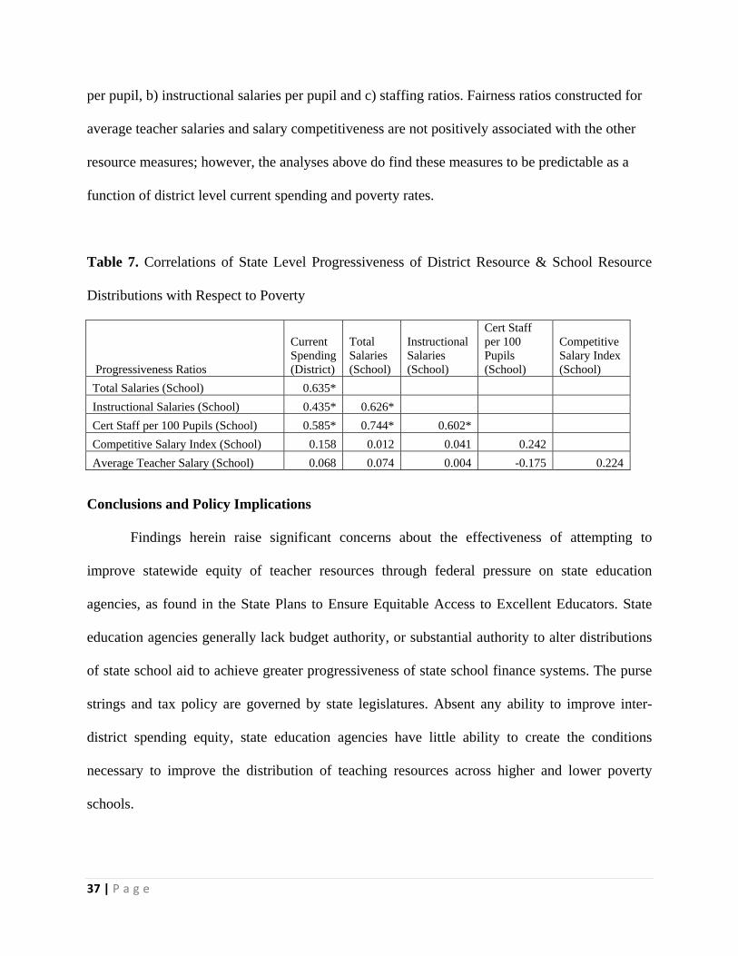
37 | P a g e
per pupil, b) instructional salaries per pupil and c) staffing ratios. Fairness ratios constructed for
average teacher salaries and salary competitiveness are not positively associated with the other
resource measures; however, the analyses above do find these measures to be predictable as a
function of district level current spending and poverty rates.
Table 7. Correlations of State Level Progressiveness of District Resource & School Resource
Distributions with Respect to Poverty
Progressiveness Ratios
Current Spending (District)
Total Salaries (School)
Instructional Salaries (School)
Cert Staff per 100 Pupils (School)
Competitive Salary Index (School)
Total Salaries (School) 0.635*
Instructional Salaries (School) 0.435* 0.626*
Cert Staff per 100 Pupils (School) 0.585* 0.744* 0.602*
Competitive Salary Index (School) 0.158 0.012 0.041 0.242
Average Teacher Salary (School) 0.068 0.074 0.004 -0.175 0.224
Conclusions and Policy Implications
Findings herein raise significant concerns about the effectiveness of attempting to
improve statewide equity of teacher resources through federal pressure on state education
agencies, as found in the State Plans to Ensure Equitable Access to Excellent Educators. State
education agencies generally lack budget authority, or substantial authority to alter distributions
of state school aid to achieve greater progressiveness of state school finance systems. The purse
strings and tax policy are governed by state legislatures. Absent any ability to improve inter-
district spending equity, state education agencies have little ability to create the conditions
necessary to improve the distribution of teaching resources across higher and lower poverty
schools.

38 | P a g e
In several large, heterogeneous states, including New York, Pennsylvania and Illinois,
districts serving more children in poverty have fewer total resources; their schools in turn have
fewer total resources, less competitive teacher compensation and less desirable staffing ratios. In
several states identified herein, district level variations in spending are significant determinants
of statewide inequity in school site resources. Thus, school site resource variation is unlikely to
be resolved by regulation, absent any correction to inter-district spending disparities. At best,
states may pressure districts to improve within-district disparities in aggregate and specific
teaching resources. While relevant and important, this policy objective misses the larger picture
of persistent disparities in total resources between local public school districts that are highly
socioeconomically and racially segregated (Baker, Sciarra & Farrie, 2015; Reardon & Owens,
2014).
Early evidence suggests that state education agency plans to comply with federal teacher
equity regulations are likely to be little more than window dressing. In the spring of 2015, we
began to see the first signs of how states intend to respond to new Federal regulations. For
example, in response to the new Federal regulations, the New York State Education Department
released a memo in April, 2015. In that memo, NYSED explained that their review of equity
profile data provided by ED revealed:
According to the USED published equity profile, the average teacher in a highest
poverty quartile school in New York earns $66,138 a year, compared to $87,161 for the
average teacher in the lowest poverty quartile schools. (These numbers are adjusted to
account for regional differences in the cost of living.) Information in the New York
profile also suggests that students in high poverty schools are nearly three times more

39 | P a g e
likely to have a first-year teacher, 22 times more likely to have an unlicensed teacher, and
11 times more likely to have a teacher who is not highly qualified.12
Despite mention of substantial salary disparities, NYSEDs proposals for improving the
distribution of teacher qualifications are paradoxically silent with respect to substantial funding
disparities that persist between the state’s higher and lower poverty school districts (Baker,
Sciarra, Farrie, 2015; Baker & Corcoran, 2012). In the portion of the memo addressing “root
causes” of disparities in qualifications, NYSED officials instead list “talent management
struggles” including: “Preparation, hiring and recruitment, professional development and growth,
selective retention, extending the reach of top talent to the most high-need students.” Indeed, the
department (NYSED) has little authority over the state school finance system that yields these
disparities.
The findings herein also raise questions regarding the validity of claims that state laws
regarding teacher tenure and due process protections are a significant cause of disparities in
teaching resources available across differing poverty and minority concentration settings. It
seems unlikely at best (or even entirely illogical) that contractual protections applied uniformly
across all local public school districts within a state could be a significant factor in creating these
disparities. Across schools and districts, student characteristics, working conditions and
resources vary, but due process requirements and tenure procedures do not. Findings herein
suggest that between district disparities in spending are a substantial determinant of total staffing
expenditures, instructional expenditures, average salaries and staffing ratios in schools. These
factors contribute to the relative competiveness of staff wages and working conditions. Coupled
12 http://www.regents.nysed.gov/meetings/2015Meetings/April/415p12hed2.pdf
40 | P a g e
with related studies showing that between-district variations in teacher qualifications are as great
or greater than within-district, cross-school variations, it seems far more likely that factors such
as spending, which vary significantly across districts, are the more likely culprits inducing
disparities in teacher attributes, and not state laws applied uniformly across districts. Findings
herein suggest as much, directly and consistently.
Put simply, the amount of funding available to any school district determines the amount
it can spend on its schools and, in turn, the combination of wage competitiveness and staffing
ratios the district can provide. Those with more can spend more; those without can’t. Where
inter-district inequities persist – especially where districts serving needier student populations
have substantially lower spending – so too will inequities in the various indicators suggested for
review by the U.S. Department of Education. Regulatory intervention without more substantive
changes to state school finance systems will likely achieve little. So too will legal challenges to
statutes and regulations which fail to correct inter-district disparities in available funding.
References Adamson, F., & Darling-Hammond, L. (2012) Funding disparities and the inequitable
distribution of teachers: Evaluating sources and solutions. Education Policy Analysis Archives, 20(37)
Retrieved [date], from http://epaa.asu.edu/ojs/article/view/1053 Ajwad, M.I. (2006) Is intra-jurisdictional resource allocation equitable? An analysis of campus
level spending data from Texas elementary schools. The Quarterly Review of Economics and Finance 46 (2006) 552-564
Andrews, M., Duncombe, W., Yinger, J. (2002). Revisiting economies of size in American education: Are we any closer to consensus? Economics of Education Review, 21, 245-262.
Baker, B. D. (2014) America’s Most Financially Disadvantaged Schools and How they Got That Way. Washington, DC. Center for American Progress. https://cdn.americanprogress.org/wp-content/uploads/2014/07/BakerSchoolDistricts.pdf
Baker, B. D. (2012). Rearranging Deck Chairs in Dallas: Contextual Constraints and Within-district Resource Allocation in Urban Texas School Districts. Journal of Education Finance, 37(3), 287-315.

41 | P a g e
Baker, B. D., Taylor, L., Levin, J., Chambers, J., & Blankenship, C. (2013). Adjusted Poverty Measures and the Distribution of Title I Aid: Does Title I Really Make the Rich States Richer?. Education Finance and Policy, 8(3), 394-417.
Baker, B. D., & Welner, K. G. (2010). Premature Celebrations: The Persistence of Inter-District Funding Disparities. education policy analysis archives, 18(9), n9.
Baker, B.D. (2009) Evaluating Marginal Costs with School Level Data: Implications for the Design of Weighted Student Allocation Formulas. Education Policy Analysis Archives 17 (3)
Baker, B. D., Sciarra, D. G., & Farrie, D. (2015). Is School Funding Fair? A National Report Card. Fourth Edition Education Law Center.
Baker, B. D., Sciarra, D. G., & Farrie, D. (2010). Is School Funding Fair? A National Report Card. Education Law Center.
Black, D. W. (2016). The Constitutional Challenge to Teacher Tenure. California Law Review, 104.
Burke, Sarah, M. 1999. “An Analysis of Resource Inequality at the State, District, and School Levels.” Journal of Education Finance, 24, 4, 435-458.
Chambers, J.G., Shambaugh, L., Levin, J., Muraki, M., Poland, L. (2008) A Tale of Two Cities: A Comparative Study of Student-Based Funding and School-Based Decision Making in San Francisco and Oakland Unified School Districts. American Institutes for Research. Palo Alto, CA.
Coley, R. J., & Baker, B. (2013). Poverty and education: Finding the way forward. Princeton, NJ: The ETS Center for Research on Human Capital and Education.
Downes, T. A. Figlio, D. N. (1999) Do Tax and Expenditure Limits Provide a Free Lunch? Evidence on the Link Between Limits and Public Sector Service Quality52 (1) 113-128
Duncombe, W., & Yinger, J. (2008). Measurement of cost differentials. Handbook of research in education finance and policy, 238-256.
Ronald Ferguson (1991) Paying for Public Education: New Evidence on How and Why Money Matters. Harvard Journal on Legislation. 28 (2) 465-498.
David N. Figlio (2002) Can Public Schools Buy Better-Qualified Teachers?” Industrial and Labor Relations Review 55, 686-699.
David N. Figlio (1997) Teacher Salaries and Teacher Quality. Economics Letters 55 267-271. Figlio, D.N., Rueben, K. (2001) Tax Limits and the Qualifications of New Teachers. Journal of
Public Economics. April, 49-71 Goldhaber, D., Lavery, L., Theobald, R. (2014) Uneven Playing Field? Assessing the Inequity of
Teacher Characteristics and Measured Performance across Students. Center for Education Data and Research. Bothel, WA. University of Washington at Bothel. http://www.cedr.us/papers/working/CEDR%20WP%202014-4.pdf
Houck, E. (2010) Teacher Quality and School Resegregation: A Resource Allocation Case Study. Leadership and Policy in Schools 9 (1) 49-77
42 | P a g e
Lankford, H., Loeb, S., & Wyckoff, J. (2002). Teacher sorting and the plight of urban schools: A descriptive analysis. Educational evaluation and policy analysis, 24(1), 37-62.
Loeb, S., Page, M. (2000) Examining the Link Between Teacher Wages and Student Outcomes: The Importance of Alternative Labor Market Opportunities and Non-Pecuniary Variation. Review of Economics and Statistics 82 (3) 393-408
Murnane, R.J., Olsen, R. (1989) The effects of salaries and opportunity costs on length of state in teaching. Evidence from Michigan. Review of Economics and Statistics 71 (2) 347-352
Ondrich, J., Pas, E., Yinger, J. (2008) The Determinants of Teacher Attrition in Upstate New York. Public Finance Review 36 (1) 112-144
Reardon, S. F., & Owens, A. (2014). 60 Years after Brown: Trends and consequences of school segregation. Annual Review of Sociology, 40, 199-218. Rebell, M.R., Baker, B.D. (2009) Assessing Success in School Finance Litigations. Education
Week Roza, M., Hawley-Miles, K. (2004) Understanding Student-based Budgeting as a Means to
Greater School Resource Equity. Center on Reinventing Public Education: University of Washington. Working Paper
Roza, M., Guin, K., Gross, B., Deburgomaster, S. (2007) Do districts fund schools fairly? Education Next. Fall, 68-73
Rubenstein, R., Schwartz, A.E., Stiefel, L., Bel Hadj Amor, Hella (2007) From districts to schools: The distribution of resources across schools in big city school districts. Economics of Education Review 26 (5) 532-545
Stiefel, L, Rubenstein, R., Berne, R. (1998) Intra-District Equity in Four Large Cities: Data, Methods and Results.” Journal of Education Finance 23, 4:447-467.
Taylor, Lori. 2004. “Adjusting for Geographic Variations in Teacher Compensation: Updating the Texas Cost-of-Education Index,” A report prepared for the Texas Legislature Joint Committee on Public School Finance, The Texas School Finance Project. Available at http://www.capitol.state.tx.us/ psf/reports.htm.
U.S. Department of Education, Office of Planning, Evaluation and Policy Development, Policy and Program Studies Service, Comparability of State and Local Expenditures Among Schools Within Districts: A Report From the Study of School-Level Expenditures, by Ruth Heuer and Stephanie Stullich, Washington, D.C., 2011.

43 | P a g e
Appendix A
Table A1
Ed Equity Files Public School Universe Data Coverage Estimate SASS Based Salary
Index Data Coverage
Estimate
State Schools Enrollment Schools Enrollment School Share
Enrollment Share Schools Enrollment
School Share
Enrollment Share
Alabama 1,296 715,618 1,343 731,725 96.5% 97.8% 152 95,862 11.3% 13.1% Alaska 482 128,500 509 131,166 94.7% 98.0% 82 21,807 16.1% 16.6% Arizona 1,833 1,030,659 2,046 1,078,249 89.6% 95.6% 131 128,453 6.4% 11.9% Arkansas 1,050 467,372 1,080 483,114 97.2% 96.7% 117 67,646 10.8% 14.0% California 9,365 6,067,005 9,893 6,202,862 94.7% 97.8% 424 478,478 4.3% 7.7% Colorado 1,757 834,909 1,810 853,669 97.1% 97.8% 122 75,369 6.7% 8.8% Connecticut 1,058 550,112 1,133 553,990 93.4% 99.3% 138 100,767 12.2% 18.2% Delaware 195 127,615 211 128,946 92.4% 99.0% 60 44,521 28.4% 34.5% District of Columbia 191 66,304 216 73,609 88.4% 90.1% 25 10,442 11.6% 14.2% Florida 3,646 2,615,008 3,920 2,668,113 93.0% 98.0% 230 245,162 5.9% 9.2% Georgia 2,253 1,656,816 2,321 1,685,016 97.1% 98.3% 140 114,695 6.0% 6.8% Hawaii 286 179,493 286 182,705 100.0% 98.2% 16 14,404 5.6% 7.9% Idaho 672 271,398 712 279,494 94.4% 97.1% 113 61,068 15.9% 21.8% Illinois 4,104 2,034,620 4,235 2,073,721 96.9% 98.1% 181 133,675 4.3% 6.4% Indiana 1,804 1,014,850 1,866 1,037,560 96.7% 97.8% 156 117,588 8.4% 11.3% Iowa 1,373 473,258 1,403 485,358 97.9% 97.5% 127 60,609 9.1% 12.5% Kansas 1,329 470,430 1,351 481,519 98.4% 97.7% 128 61,058 9.5% 12.7% Kentucky 1,341 666,217 1,409 681,643 95.2% 97.7% 160 87,674 11.4% 12.9% Louisiana 1,341 666,595 1,415 702,301 94.8% 94.9% 123 80,276 8.7% 11.4% Maine 614 173,079 579 178,989 106.0% 96.7% 85 36,990 14.7% 20.7% Maryland 1,383 849,176 1,422 854,295 97.3% 99.4% 68 53,273 4.8% 6.2% Massachusetts 1,770 928,826 1,829 953,369 96.8% 97.4% 120 87,012 6.6% 9.1% Michigan 3,257 1,463,719 3,514 1,533,660 92.7% 95.4% 235 140,751 6.7% 9.2% Minnesota 1,808 765,971 2,186 839,645 82.7% 91.2% 220 157,645 10.1% 18.8% Mississippi 868 474,942 899 490,619 96.6% 96.8% 94 60,788 10.5% 12.4% Missouri 2,200 897,145 2,269 916,300 97.0% 97.9% 189 109,795 8.3% 12.0% Montana 789 137,716 826 142,409 95.5% 96.7% 69 29,817 8.4% 20.9% Nebraska 988 294,883 1,009 301,296 97.9% 97.9% 136 67,891 13.5% 22.5% Nevada 616 434,314 642 439,128 96.0% 98.9% 100 109,804 15.6% 25.0% New Hampshire 464 184,248 476 191,012 97.5% 96.5% 47 37,709 9.9% 19.7% New Jersey 2,394 1,324,287 2,471 1,352,571 96.9% 97.9% 188 156,629 7.6% 11.6% New Mexico 797 325,813 855 335,236 93.2% 97.2% 111 69,658 13.0% 20.8% New York 4,513 2,651,363 4,647 2,702,503 97.1% 98.1% 154 115,900 3.3% 4.3% North Carolina 2,457 1,471,917 2,508 1,499,541 98.0% 98.2% 129 79,167 5.1% 5.3% North Dakota 492 94,792 476 97,534 103.4% 97.2% 109 41,848 22.9% 42.9%
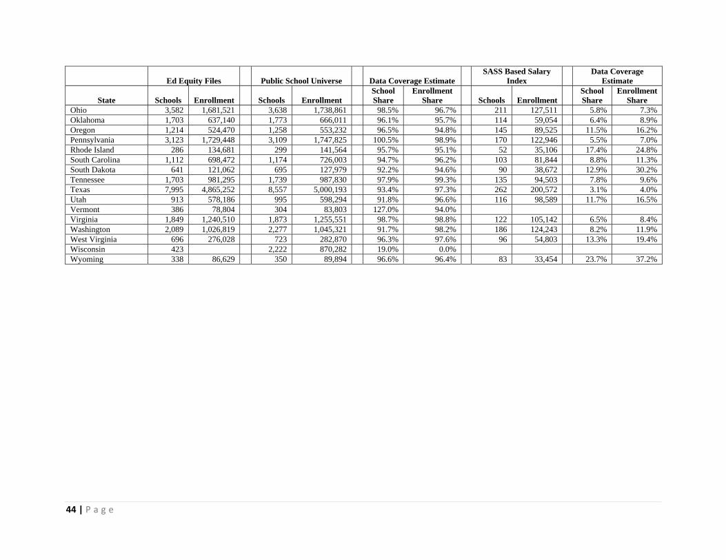
44 | P a g e
Ed Equity Files Public School Universe Data Coverage Estimate SASS Based Salary
Index Data Coverage
Estimate
State Schools Enrollment Schools Enrollment School Share
Enrollment Share Schools Enrollment
School Share
Enrollment Share
Ohio 3,582 1,681,521 3,638 1,738,861 98.5% 96.7% 211 127,511 5.8% 7.3% Oklahoma 1,703 637,140 1,773 666,011 96.1% 95.7% 114 59,054 6.4% 8.9% Oregon 1,214 524,470 1,258 553,232 96.5% 94.8% 145 89,525 11.5% 16.2% Pennsylvania 3,123 1,729,448 3,109 1,747,825 100.5% 98.9% 170 122,946 5.5% 7.0% Rhode Island 286 134,681 299 141,564 95.7% 95.1% 52 35,106 17.4% 24.8% South Carolina 1,112 698,472 1,174 726,003 94.7% 96.2% 103 81,844 8.8% 11.3% South Dakota 641 121,062 695 127,979 92.2% 94.6% 90 38,672 12.9% 30.2% Tennessee 1,703 981,295 1,739 987,830 97.9% 99.3% 135 94,503 7.8% 9.6% Texas 7,995 4,865,252 8,557 5,000,193 93.4% 97.3% 262 200,572 3.1% 4.0% Utah 913 578,186 995 598,294 91.8% 96.6% 116 98,589 11.7% 16.5% Vermont 386 78,804 304 83,803 127.0% 94.0% Virginia 1,849 1,240,510 1,873 1,255,551 98.7% 98.8% 122 105,142 6.5% 8.4% Washington 2,089 1,026,819 2,277 1,045,321 91.7% 98.2% 186 124,243 8.2% 11.9% West Virginia 696 276,028 723 282,870 96.3% 97.6% 96 54,803 13.3% 19.4% Wisconsin 423 2,222 870,282 19.0% 0.0% Wyoming 338 86,629 350 89,894 96.6% 96.4% 83 33,454 23.7% 37.2%