Intelligent Transformer MonitoringSystem Utilizing Neuro-Fuzzy

Technique Approach

Intelligent Substation Final Project Report

Power Systems Engineering Research Center

A National Science FoundationIndustry/University Cooperative Research Center

since 1996

PSERC

Power Systems Engineering Research Center

Intelligent Transformer Monitoring System Utilizing Neuro-Fuzzy Technique

Approach

Final Project Report

Intelligent Substation

Project Team

Rahmat Shoureshi, Project Leader Tim Norick

Ryan Swartzendruber

Colorado School of Mines

PSERC Publication 04-26

July 2004

Information about this project For information about this project contact: Rahmat Shoureshi, Ph.D. University of Denver Dean of School of Engineering and Computer Science 2050 E. Iliff Ave. Boettcher Center East, Rm. 227 Denver, CO 80208 Tel: 303-871-2621 Fax: 303-871-2716 Email: rshoures@du.edu Power Systems Engineering Research Center This is a project report from the Power Systems Engineering Research Center (PSERC). PSERC is a multi-university Center conducting research on challenges facing a restructuring electric power industry and educating the next generation of power engineers. More information about PSERC can be found at the Center’s website: http://www.pserc.org For additional information, contact: Power Systems Engineering Research Center Cornell University 428 Phillips Hall Ithaca, New York 14853 Phone: 607-255-5601 Fax: 607-255-8871 Notice Concerning Copyright Material PSERC members are given permission to copy without fee all or part of this publication for internal use if appropriate attribution is given to this document as the source material. This report is available for downloading from the PSERC website.

© 2004 Colorado School of Mines. All rights reserved.

Acknowledgements

The work described in this report was sponsored by the Power Systems Engineering

Research Center (PSERC). We express our appreciation for the support provided by PSERC’s

industrial members and by the National Science Foundation under a grant received under the

Industry/University Cooperative Research Center Program.

We would also like to express our sincere appreciation to the Western Area Power

Administration and its employees for their support of this project. The use of their substation for

testing of our module was essential to project success.

We would specifically like to thank John Work for his ongoing support and time throughout

our work on this project. We would never have been able to succeed in this project without his

help.

Executive Summary

Maintaining the health and reliability of the power substation has been a concern for many

years. For this reason, maintenance crews would periodically take transformers and circuit

breakers off-line, in order to assess whether the equipment is operating normally. With this

method, there are still catastrophic failures, not to mention much unneeded maintenance. With a

growing need for lower cost and more efficient diagnostic tools, the advent of on-line monitoring

and artificial intelligence analysis techniques have been applied to the electrical power

substation. This report details development of an advanced predictive maintenance and

diagnostic system that can be used to monitor the health of the transformer and other substation

equipment. Thus, maintenance can be performed on a needed rather than scheduled basis.

A portable, on-line diagnostic module is designed that is able to collect current, temperature,

and vibration data from non-invasive sensors, condition the signals appropriately, send the data

to the substation computer for storage, and then have the ability to remotely access the data for

analysis and health assessment. An artificial intelligent architecture utilizing neuro-fuzzy

techniques is used for non-linear system identification, output estimation, and fault detection.

Experimental results are presented from the application of the diagnostic module and neuro-

fuzzy system on three, single-phase 166 MVA transformers. The system has been successfully

able to identify the equipment dynamics, estimate the outputs, and detect a simulated thermal

fault, as well as distinguish between sensor and system failures. The foundation for a hybrid

neuro-fuzzy expert system is also detailed. The potential for transformer and substation

equipment health diagnosis and life expectancy prediction using this system is immense.

ii

Table of Contents 1. Introduction………….…………………………………………………..……………. 1 1.1 Motivation……………...…………………………………………………………... 1 1.2 Research Objective………………………………………………………………….2 1.3 Report Outline……………………………………………………………………… 3

2. Literature Review……………………………………………………………………...5 2.1 Diagnostic Hardware………………………………………………………………. 5 2.1.1 Dissolved Gas Analysis…………………………………………………...……5 2.1.2 Moisture Analysis………………………………………………………………8 2.1.3 Partial Discharge Monitoring…………………………………………………. 8 2.1.4 Temperature Monitoring……………………………………………………… 10 2.1.5 Vibration Monitoring…………………………………………………………. 11 2.1.6 Current Monitoring…………………………………………………………… 12 2.1.7 Bushing and CT Monitoring………………………………………………….. 12 2.1.8 LTC Monitoring………………………………………………………………. 13

2.2 Approaches to Fault Detection…………………………………………………….. 14 2.2.1 Fault Diagnosis Methods…………………………………………………...… 14 2.2.2 Analytic Models for Transformer Diagnostics……………………………….. 16 2.2.3 Artificial Intelligence Diagnosis of Transformers……………………………. 19

3. Neuro-fuzzy Fault Detection Engine………………………...…………………….… 24 3.1 Overview of Diagnostic Approach………………………………………………... 25 3.2 Non-linear System Identification………………………………………………….. 26 3.2.1 Background of Neural Networks for System Identification………………….. 27 3.2.2 Neural Network Architectures……………………………………………...… 30 3.2.3 TNFIN Architecture…………………………………………………………... 31 3.2.4 Hybrid Learning Algorithm…………………………………………………... 34

3.3 Neural-Based Non-linear Observer………………………………………………... 36 3.3.1 Observer Introduction and Background………………………………………. 36 3.3.2 Non-linear Observer Using Neural Network Dynamic Models……………… 38 3.3.2.1 Newton’s Methods…………………………………………………………... 41 3.3.2.2 Levenberg-Marquardt Method………………………………………………. 41

3.4 Fault Detection…………………………………………………………………….. 43 3.4.1 Background of Fault Detection Approaches………………………………….. 44 3.4.2 Observer Residual Generation………………………………………………... 45 3.4.3 Optimization Based Fault Detection Approach………………………………. 47 3.4.4 Non-linear System Fault Detection…………………………………………… 51

iii

Table of Contents (continued) 4. Design and Construction of the Monitoring System……………………………..…... 52 4.1 Sensor Node……………………………………………………………………….. 54 4.2 Signal Conditioning Node…………………………………………………………. 57 4.3 DAQ, Storage, and Transmittal Nodes……………………………………………. 59 4.4 Portable Experimental Module……………………………………………………. 60 4.5 Data Analysis Node……………………………………………………………….. 62 4.6 Interface Node……………………………………………………………………... 63 4.7 Field Implementation……………………………………………………………… 64

5. Foundation for Future Transformer Monitoring System…………………………...... 65 5.1 Background…....…………………………………………………………………... 65 5.2 Dissolved Gas Analysis Thresholds…………………………………………….…. 66 5.3 Moisture Analysis Limits………………………………………………………..… 67 5.4 Top Oil Temperature Thresholds………….…………..…………………………... 67 5.5 Vibration Levels………………………..………………………………………….. 69 5.6 Bushing Thermal Thresholds……………………………………………..……….. 69 5.7 LTC thermal Thresholds…………………………..………………………………. 70 5.8 Fusion into Expert System……………………………..………………………….. 71 5.9 Proposed Hybrid Diagnostic System…………..………………………………….. 72

6. Experimental Analysis……………………………………………………………….. 74 6.1 Off-line Fault Detection Analysis……………………………………………….… 74 6.2 Non-linear System Identification………………………………………………….. 75 6.3 Model Validation and Output Estimation…………………………………………. 89 6.4 Fault Detection…………………………………………………………………… 92 6.4.1 System Failure………………………………………………………………. 92 6.4.2 Sensor Failure……………………………………………………………….. 95

6.4.3 System and Sensor Failure…………………………………………………... 96 7. Conclusions and Future Work……………………………………………………… 99 7.1 Summary…………………………………………………………………………. 99 7.1.1 Diagnostic Hardware Module……………………………………………….. 99 7.1.2 Data Manipulation and Communication…………………………………….. 100 7.1.3 Non-linear System Identification and Fault Detection……………………… 100 7.1.4 Hybrid Neuro-fuzzy Expert System…………………………………………. 101

7.2 Future Work…………………………………………………………………….... 101 8. References……...………………………………………………………………….... 104

iv

Table of Figures . Figure 1.1: Typical large substation transformer……………………………………... 4 Figure 2.1: Various approaches to fault diagnosis…………………………………….... 15 Figure 2.2: Model-based monitoring scheme for transformer………………………….. 17 Figure 2.3: Comparison between white and black box diagnostics…………………….. 20 Figure 2.4: Strategy for combined fuzzy logic, expert system, and neural network…… 21 Figure 2.5: Fault Diagnosis method utilizing neural network moisture data…………… 23 Figure 3.1: Block diagram of diagnostic approach…………………………………...… 26 Figure 3.2: Process of system identification……………………………………………. 27 Figure 3.3: Architecture of the TNFIN.………………………………………………… 33 Figure 3.4: Block diagram for on-line observer with residual generation……………… 46 Figure 3.5: Comparison for degrees of observability………………………………...… 47 Figure 4.1: Comparison between distributed and centralized systems……………….… 53 Figure 4.2: Magnetic mount temperature sensor placed on test transformer…………… 55 Figure 4.3: Industrial accelerometer used to measure shell vibration………………….. 56 Figure 4.4: Current transformer used to monitor currents in coils, pumps, and fans…... 57 Figure 4.5: Two circuits used in implementation of signal conditioner………………... 59 Figure 4.6: Versalogic PC104 and DAQ card used for the storing and transmittal of Data…………………………………………………………………………. 60 Figure 4.7: Designed portable diagnostic module with PC104 and signal conditioner.... 61 Figure 4.8: Diagnostic module mounted inside transformer cabinet…………………… 61

v

Table of Figures (continued) Figure 4.9: Steps taken to transfer sensor data to PC with ANN……………………….. 62 Figure 4.10: Sample GUI interface on substation computer……………………………. 63 Figure 4.11: Three single-phase 166 MVA transformers used in experiment………….. 64 Figure 5.1: Block Diagram of Hybrid Diagnostic Approach…………………………… 74 Figure 6.1: Four membership functions of Transformer A’s top tank temperature input………………………………………………………………………... 76 Figure 6.2: Transformer A system input-top tank temperature………………………… 78 Figure 6.3: Transformer A system input-ambient temperature………………………… 78 Figure 6.4: Transformer A system input-primary current……………………………… 79 Figure 6.5: Transformer A system input-secondary current………………………….… 79 Figure 6.6: Transformer A system input-tertiary current…………………………….…. 80 Figure 6.7: Transformer A system input-fan and pump bank current #1…………….… 80 Figure 6.8: Transformer A system input-fan and pump bank current #2………………. 81 Figure 6.9: Transformer A system input-7th harmonic vibration……………………… 81 Figure 6.10: Transformer A system input-9th harmonic vibration………………….….. 82 Figure 6.11: Transformer A system output-main tank temperature…………………….. 82 Figure 6.12: Transformer A system output-3rd harmonic vibration………………….… 83 Figure 6.13: Transformer A system output-5th harmonic vibration……………………. 83 Figure 6.14: Transformer A TNFIN training versus actual-main tank temperature……. 85 Figure 6.15: Transformer A TNFIN training versus actual-3rd harmonic vibration…… 85

vi

Table of Figures (continued) Figure 6.16: Transformer A TNFIN training versus actual-5th harmonic vibration…… 86 Figure 6.17: Transformer B TNFIN training versus actual-main tank temperature……. 86 Figure 6.18: Transformer B TNFIN training versus actual-3rd harmonic vibration…… 87 Figure 6.19: Transformer B TNFIN training versus actual-5th harmonic vibration…… 87 Figure 6.20: Transformer C TNFIN training versus actual-main tank temperature……. 88 Figure 6.21: Transformer C TNFIN training versus actual-3rd harmonic vibration…… 88 Figure 6.22: Transformer C TNFIN training versus actual-5th harmonic vibration…… 89 Figure 6.23: Transformer A neural network validation……………………………….... 90 Figure 6.24: Transformer B neural network validation………………………………… 90 Figure 6.25: Transformer C neural network validation………………………………… 91 Figure 6.26: Recognition time for neural network training of transformer A………… 92 Figure 6.27: Result of fault detection for transformer A……………………………… 94 Figure 6.28: Result of fault detection for transformer B……………………………… 94 Figure 6.29: Result of fault detection for transformer C……………………………… 95 Figure 6.30: V1 sensor failure, detection and isolation of sensor failure……………... 97 Figure 6.31: Detection and isolation and system and sensor failure………………….. 98

vii

List of Tables Table 2.1: Key gases for DGA and their fault type……………………………………… 6 Table 5.1: Concentration (ppm) for dissolved key gases……………………………….. 67 Table 5.2: Warning categories for top oil temperature…………………………………. 68 Table 5.3: Warning categories for top oil temperature above reference………………... 68 Table 5.4: Warning categories for shell vibration readings…………………………….. 69 Table 6.1: Input output measurements used for transformer models…………………… 77 Table 6.2: Summary of training results for three transformers (A-C)………………….. 84

viii

1. Introduction This introductory chapter describes the importance of this research topic, its impact, and the

goals and objectives of the project. A short outline for the rest of the report is also provided.

1.1 Motivation In recent years, increased emphasis has been placed on power reliability. In particular, major

changes in the utility industry, primarily caused by restructuring and re-regulation, have caused

increased interest in more economical and reliable methods to generate and transmit power. The

health of equipment constituting the substation is critical to assuring that the supply of power can

meet the demand. As has been seen recently in California and more dramatically in the recent

blackout in the northeast, the United States is already beginning to reach a point where the

transmission and distribution system cannot handle the instantaneous demanded power load.

The equipment making up the foundation of a substation, primarily circuit breakers and

transformers, are expensive, as is the cost of power interruptions. The savings that would be

accrued from the prevention of failures in substation equipment would be in the millions of

dollars (Cournoyer, 1999). In the past, most maintenance of large substation transformers was

done based on a pre-determined schedule. Maintenance crews would inspect a transformer at set

intervals based on its past age and performance history. As can be expected, this leads to many

catastrophic failures of improperly diagnosed transformers and the over inspection of other

healthy transformers. Because of the cost of scheduled and unscheduled maintenance, especially

at remote sites, the utility industry had begun investing in instrumentation and monitoring of

substation equipment. On-line transformer diagnostics is the key to greatly reducing the cost and

increasing the reliability of providing the needed electrical energy to a growing society. In this

report, the on-line monitoring and health diagnostics of transformers is investigated.

Transformers are the most expensive piece of equipment in the substation and; therefore,

preventing transformer failures is critical. Transformers are continuing to become larger and

1

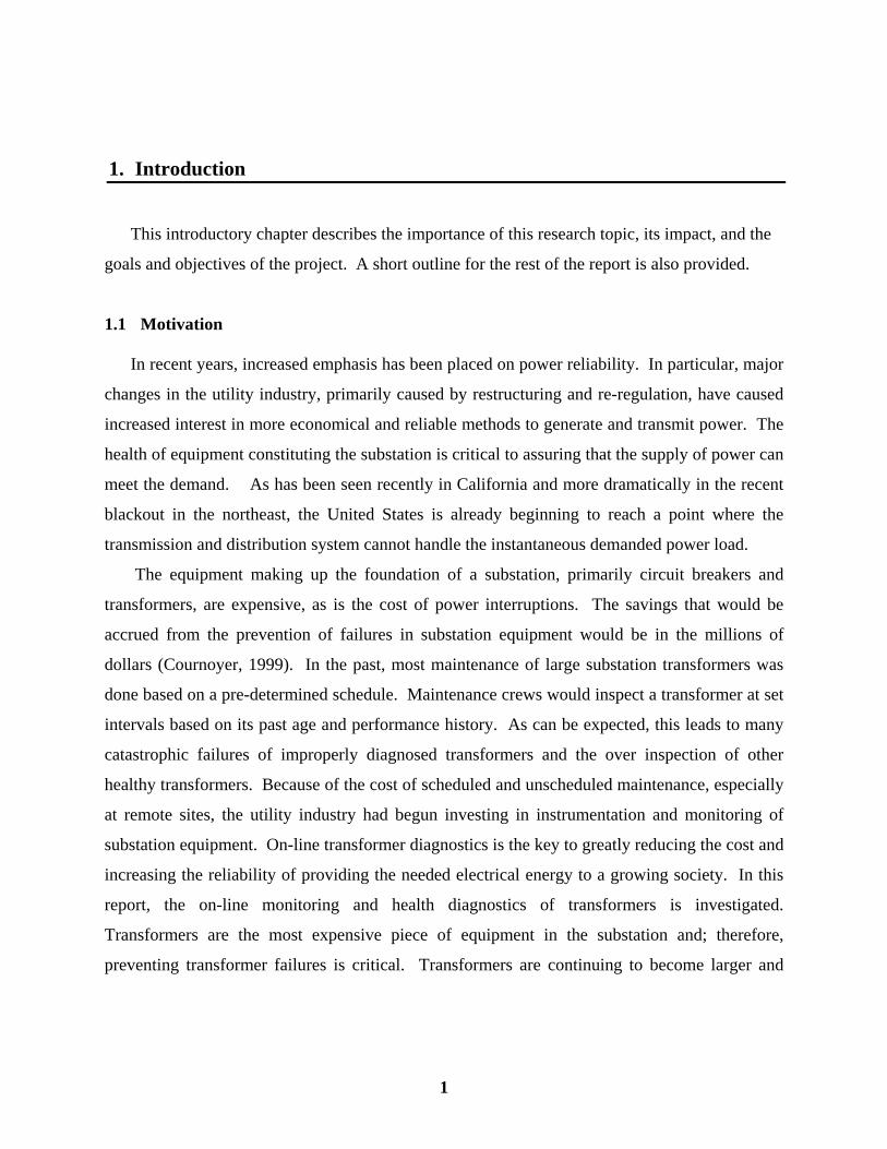
larger with some handling over 1000 MVA (see Figure 1.1). For this reason, assuring power

reliability entails the proper running of these transformers.

1.2 Research Objective The main objective of this research is to develop the foundation of an intelligent substation in

terms of self-diagnostic, self-data analysis and self-informing equipment. While the fundamental

and analytical techniques for an intelligent substation are presented, the results are implemented

on real-life transformers for an actual substation. The purpose of this research is to develop a

sample diagnostic system that outlines the sensors needed and the analytical software used to

extract information about the health of the large substation transformer from this sensor data.

This system needs to be able to collect and manipulate the data from the sensors, send it to the

substation host computer, and then be able to remotely access from a maintenance computer that

can perform the automatic fault detection. The goal is then to use the neuro-fuzzy system to

identify equipment dynamics through training to a sample data set. It will then be shown how

the system can detect failures and distinguish between system failures and sensor failures. This

diagnostic system would be implemented on a set of large 166 MVA transformers. A large set of

sample data will be collected that can be used as a baseline for future expansion of the diagnostic

system to multiple substations. In addition, the foundation for an expert system developed based

on the latest transformer expertise will be described that can complement the neuro-fuzzy

diagnostic system. This foundation sorts through the many different possible sensor thresholds

that could be used in an expert system and details the most used and accepted thresholds.

The on-line monitoring of transformers or other substation equipment is only part of what is

needed for fault detection. The sensors merely provide massive quantities of real time data.

Thus, a mechanism is needed for analyzing this data and providing useful diagnostic information

about the health of the equipment. The analysis can be as simple as placing certain limits and

thresholds on the range of sensor measurements. This is a simple method that can prove helpful

for certain conditions. However, when the system that is being monitored is more complex and

2

exhibits non-linear dynamic behavior, as a transformer does, simple threshold analysis is not

sufficient. In this case, more sophisticated methods should be employed. This is because

dynamic systems have changing relationships between the system variables that characterize

both normal and faulted states. For example, a certain temperature rise may be a sign of

impending failure in a new transformer but not in an older one. The problem then becomes how

to symbolize these changing relationships in a practical and reliable way.

As systems become more complex and interconnected, it becomes difficult to maintain

them. Components wear and fail, or operating conditions change, causing performance

degradation. To meet this challenge, fault detection and isolation strategies have been developed

over the past decades to enable automatic detection of faulty conditions, so that measures can be

taken before the failure becomes catastrophic. In the case of large power transformers (see

Figure 1.1), a catastrophic failure costs millions of dollars. Thus, there is a real need to be able

to monitor these transformers and set alarms if there are any impending failures. This should be

done with the minimum number of sensors, while still providing reliable diagnostic information.

This research attempts to accomplish the goal of an affordable and reliable system that can easily

be installed to monitor large transformers. Results form this research can be expanded to circuit

breakers, a complete substation, and a transmission and distribution system.

1.3 Report Outline

This report will begin with an extensive review of the current techniques and diagnostic

hardware that are being used for transformer monitoring. There will also be a comprehensive

review of the different types of analytical methods that have been developed over the years and

how they can be used to provide diagnostic information from large volumes of data. In addition

to analytical methods, common artificial intelligence techniques for transformer diagnostics will

be discussed. These topics will be overviewed in Chapter 2. Chapter 3 describes the neuro-

fuzzy network that is used to analyze and extract diagnostic information from the data collected

by the diagnostic module of Chapter 4. In Chapter 3, the ability of the neural network to act as a

3

non-linear system identifier, an output observer, and a fault detector is illustrated. Chapter 4

gives a detailed description of the diagnostic module that was designed for this research.

Figure 1.1: Typical large substation transformer A rule-base of thresholds for the different types of sensors used in transformer diagnostics,

including those sensors not implemented in the diagnostic system of Chapter 4, is formed in

Chapter 5. These thresholds are derived from the latest expert experience with transformer

diagnostics and can later be used in the implementation of an expert system. Chapter 6 gives the

experimental analysis from the application of the diagnostic module and analytical neuro-fuzzy

system. The optimal location of sensors and determination of the appropriate inputs and outputs

for the analytical system are given in this chapter and applied to the field data to illustrate the

proper functioning of the diagnostic system. Finally, a summary of the results from this report,

the future work planned for this research, and conclusions are provided in Chapter 7.

4

2. Literature Review The area of substation diagnostics, and in particular transformer diagnostics, has become

increasingly important in recent years with more and more strain being placed on the

transmission and distribution (T & D) system. A key component for the reliability of a T & D

system is the transformer. Much effort has been made in recent years to formulate techniques to

diagnose the health of transformers. The work presented in this thesis centers around three major

areas of study in transformer diagnostics. These three main areas can be divided into diagnostic

hardware and what failures they indicate, expert system with a rule-base of if-then statements for

different types of failures, and artificial intelligence that can be used as a system identifier, non-

linear observer, and fault detector. The predominant literature on these three areas is discussed

in this chapter and in Chapter 5.

2.1 Diagnostic Hardware

In recent years, many new devices have been developed to help in providing information that

can be used in diagnosing the health of transformers. There are many key measurements that can

help in indicating if a transformer is healthy or not. These measurements include the water in

oil, combustible gas in oil, temperature, gas pressure, insulation properties, partial discharge,

acoustic signatures, motor current profiles, bushing leakage current detection, moisture in

insulation, spectral content of shell vibration, and load current and voltage (Farquharson, 2000).

The above quantities can all help in detection of many different types of failures. An explanation

of the quantities, what they infer about the health of a transformer, and the common hardware

used to obtain the above quantities is given below.

2.1.1 Dissolved Gas Analysis Dissolved gas analysis has become a very popular technique for monitoring the overall health

of a transformer. As various faults develop, it is known that different gases are generated. By

5

taking samples of the mineral oil inside a transformer, one can determine what gases are present

and their concentration levels. Work has been done to theoretically connect the gaseous

hydrocarbon formation with the thermodynamic equilibrium (Halstead, 1973). Work by

Haltstead indicated that the hydrocarbon gases with the fastest rate of evolution would be

methane, ethane, ethylene, and acetylene. Halstead’s work further proved that there is a

relationship between fault temperature and the composition of the gases dissolved in the oil.

Much effort has been made into creating a diagnosis criteria for the types and amounts of gases

that are present in the oil (Zhang et al., 1996).

Some studies have focused on key gases and what faults they can be used to identify (Griffin,

1988). A summary of the relationship between fault types and the key gases is given in Table

2.1.

Table 2.1: Key gases for DGA and their fault type

Key Gas Chemical

Symbol

Fault Type

Hydrogen H2 Corona Carbon Monoxide and

Carbon Dioxide CO CO2

Cellulose insulation Breakdown

Methane and Ethane

CH4 C2H6

Low temperature Oil breakdown

Acetylene C2H2 Arcing Ethylene C2H4 High temperature oil breakdown

In the case of key gas analysis, a fault condition is indicated when there is excessive

generation of any of these gases. For this to be effective, much expert experience is still needed.

As an alternative, research has been done in the area of the ratios between different gases. In this

method, the ratio between the concentrations of different dissolved gases is used for the fault

diagnosis. For example, acetylene concentrations that exceed the ethylene concentrations

indicate that extensive arcing is occurring in the transformer, since arcing produces acetylene

(Ward, 2001a). Extensive arcing is a sign of insulation degradation and possible failure in the

6

transformer. Likewise, there are many other ratios that can be used. The problem with ratio

analysis is the knowledge base that is required to properly diagnose a transformer from the ratio

of its dissolved gases must be very large and complex (Zhang et al., 1996).

In addition to key gas analysis and ratio methods, researchers have developed a formula for

the equivalent gas content in the oil, which weights the amount of hydrogen, carbon monoxide,

acetylene, and ethylene present in the oil to produce a single number. This number can then be

used to identify abnormal conditions when comparing it to some pre-determined threshold value.

A set of standards for limits on these gases has been created and will be discussed in more detail

in the rule-base section of Chapter 5. The trends in the gases is often more important than the

absolute concentrations and many dissolved gas sensors have a trending algorithm that will put

more emphasis on abrupt changes in concentrations, especially in the key gases such as

acetylene.

Several different dissolved gas sensors have been created. The most commonly used on-line

dissolved gas analyzer is the Hydran by GE-Syprotec. It detects six of the major dissolved gases

present in the oil. In addition, it is programmed with a trending algorithm for assistance with

transformer diagnostics. The Hydran detects the hydrogen, carbon monoxide, acetylene, and

ethylene content in the oil. It connects directly to the load tap changer and provides daily values

and trending information (Reason, 1995). Besides the Hydran, Severon makes a TrueGas on-line

analyzer as does Morgan Shaffer. Morgan Shaffer’s online analyzer also monitors the water

content in the oil, which we shall discuss next. Advanced Optical Controls, Inc has developed a

more complicated gas analyzer. Advanced sensor monitors the actual concentration of six gases

using near infrared spectroscopy. Samples can be taken every half hour and an associated

microprocessor can store data for up to two months. It should be noted that the aforementioned

types of sensors and monitoring systems cost several thousand dollars each, with prices ranging

from a little over $6000 to nearly $17000 (Reason, 1996).

7

2.1.2 Moisture Analysis In addition to gas in the oil, it is an accepted fact that the presence of water is not healthy for

power transformers. Water in the oil indicates paper aging, since the cellulose insulation used in

power transformers is known to produce water when it degrades (Ward, 2001b). Water and

oxygen in the mineral oil further increases the rate at which the insulation will degrade. This

means that a high concentration of water in the oil not only indicates that the insulation has been

degrading but it will degrade more quickly in the future due to increased presence of water in the

oil. Water in the oil is also a sign that the mineral oil itself is deteriorating. When the mineral

oil deteriorates, the dielectric constant of the oil decreases. Reduction of the dielectric constant

can lead to a flashover and consequential failure of the transformer.

The relationship between the oil in the mineral oil and the insulation paper is a complex

equilibrium. Water is constantly moving from the oil to the insulation and vise-versa. The

migration of water inside the transformer is a very complicated process (Ward, 2001b). Work

has been done using a fuzzy-logic identification tool to detect the water-in-paper activity. This

tool then takes into account the moisture available for transfer to the oil. On-line measurements

of the water saturation in the oil, top and bottom oil temperatures, and load are used to determine

this activity (Davydov, 1998).

As with the dissolved gas analyzer, several companies make on-line moisture sensors that

give measurements of the amount of water present in the oil. One of the most commonly used is

the Aquaoil by GE-Syprotec. Other companies also have moisture-in-oil analyzers, such as

Doble’s Domino. These moisture-in-oil sensors cost around $5000 each.

2.1.3 Partial Discharge Monitoring Though moisture and dissolved gas analysis is helpful in detecting many types of failures that

can occur in a transformer, the measurement of partial discharges is probably the most effective

method to detect pending failure in the electrical system (Ward, 2001b). As the electrical

insulation in a transformer begins to degrade and breakdown, there are localized discharges

8

within the electrical insulation. Every discharge deteriorates the insulation material by the

impact of high-energy electrons, thus causing chemical reactions. During these discharges, ultra-

high frequency waves are emitted. Most incipient dielectric failures will generate numerous

partial discharges before the catastrophic electrical failure. Partial discharges may occur only

right before failure but may also be present for years before any type of failure. A high

occurrence of partial discharges can indicate voids, cracking, contamination, or abnormal

electrical stress in the insulation (Ward, 2001b). Because of the importance that partial discharge

measurements have in diagnosing potential catastrophic failures in a transformer, it is critical that

partial discharge measurements be able to be made in the field.

At first, techniques to be able to detect partial discharges were few and far between. Luckily,

because of the ultra-high frequency (UHF) waves produced during partial discharge, sensors

have been developed that use UHF couplers to detect frequencies from 300-1500 MHz. Scottish

Power and Strathclyde University first developed these types of sensors (Judd, 2000). In

addition to UHF sensors, the UHF waves produced by the partial discharge produce pressure

waves that are transmitted through the oil medium. Piezoelectric sensors can be used to detect

these waves. These sensors can be placed on the outside of the tank to detect the acoustic wave

impinging on the tank or in it, and the oil itself. The problem with placing it in the oil is that the

sensor than becomes invasive. The external and internal partial discharge sensors both cost

about $2000 each.

The advantage of partial discharge sensors is the ability to detect the actual location of

insulation deterioration, unlike with dissolved gas sensors. By placing several partial discharge

sensors around the transformer tank, it becomes possible to pinpoint the exact location of the

discharges (Reason, 1995). Most often the deterioration occurs on the first several coils of the

high side voltage of the transformer. The one disadvantage to partial discharge sensors is that

they are greatly affected by the electromagnetic interference in the substation environment.

Therefore, signal processing techniques are often used to improve the signal to noise ratio in

order to make the measurements effective (Bengtsson, 1997).

9

Another on-line partial discharge detection technique that involves a fiber optic sensor has

been developed recently at Virginia Polytechnic Institute and State University.

In this technique, a laser diode transmits light into a fiber optic coupler that has the light

propagate across an air gap inside a self-contained diaphragm, lined with reflective gold. The

reflected light combines with the small, reflected wave inside the fiber optic coupler to produce

an interference pattern that differs as the air gap changes. In this way, the acoustic waves

produced by partial discharges can be detected (Wang, 2000).

2.1.4 Temperature Monitoring One of the simplest and most effective ways to monitor a transformer externally is through

temperature sensors. Abnormal temperature readings almost always indicate some type of

failure in a transformer. For this reason, it has become common practice to monitor the hot spot,

main tank, and bottom tank temperatures on the shell of a transformer.

It is known that as a transformer begins to heat up, the winding insulation begins to

deteriorate and the dielectric constant of the mineral oil begins to degrade. Likewise, as the

transformer heats, insulation deteriorates at even a faster rate. As the next section describes,

monitoring the temperature of the load tap changer (LTC) is critical in determining if a LTC

would fail. In addition to the LTC, abnormal temperatures in the bushings, pumps, and fans can

all be signs of impending failures.

Recently, thermography has been used more widely for detecting temperature abnormalities

in transformers. In this technique, an infrared gun is taken to the field and used to detect

temperature gradients on external surfaces of the transformer. Infrared guns make it easy to

detect whether a bushing or fan bank is overheating and needs to be replaced. The method is

also useful in determining whether a load tap changer (LTC) is operating properly (this will be

discussed more in the section on LTC monitoring). Thermography is effective for checking

many different transformers quickly to see if there is any outstanding problem (Kirtley, 1996).

10

However, thermography is not conducive to on-line measurements and; therefore, is prone to

miss failures that may be developing between the periods when the transformers are checked.

In order to make on-line monitoring possible, thermocouples are placed externally on the

transformer and provide real-time data on the temperature at various locations on the

transformer. In many applications, temperature sensors have been placed externally on

transformers in order to estimate the internal state of the transformer. These temperature

readings can be used to determine whether the transformer windings and oil are overheating or

running at abnormally high temperatures. High main tank temperatures have been known to

indicate oil deterioration, insulation degradation, and water formation (Kirtley, 1996).

The state of the art currently in thermal detection comes in the form of transformer models.

Mathematical models have been used to accurately predict oil and winding temperature for

varying conditions, using exclusively external thermal detectors. The parameters for these

models include main tank temperature, hot spot temperature, and ambient temperature. The

IEEE had developed a model, but did not properly account for changes in the ambient

temperature and thus set off alarms when there was no fault. In the past several years,

researchers at MIT have developed a model that accurately predicts the thermal state of a

transformer (Lesieutre, 1997). Here at CSM, we have also developed a thermal model, which

used extended Kalman filters and adaptive Hopfield networks in order to develop an observer

that could estimate the state of the transformer from a few temperature measurements. The

Kalman filter and Hopfield networks were used to calculate various parameters, which could be

used to estimate the state of the transformer and determine whether it was in a failure mode

(Ottele, 1999).

2.1.5 Vibration Monitoring The diagnostic methods described thus far have all dealt with trying to detect a failure in the

electrical subsystem of the transformer, namely the electrical insulation around the coils. There

has also been research carried out in regards to mechanical malfunctions in a transformer. The

11

cellulose insulation on the coils of the transformer shrinks with aging. The shrinkage causes a

loosening in the clamping pressure. If the coils are not retightened, the decreased pressure can

often lead to a short-circuit between turns (Berler et al., 2000). Short circuits often can lead to

the catastrophic failure of the transformer and thus must be monitored closely. Studies of

transformer breakdowns have shown that between 70 and 80% of failures are caused by a short

circuit between turns in the transformer.

2.1.6 Current Monitoring Though not part of the new diagnostic tools that have been developed recently, monitoring

the currents on the primary, secondary, and tertiary coils has been done for quite a while. In

addition, monitoring the current being drawn by the fans and pumps can also indicate when there

might be a failure in these accessory units. Monitoring these currents may often be an easier and

cheaper alternative than thermography or other types of thermal monitoring. It is important to

monitor the appropriate functioning of the cooling system. Should a fan bank fail and not be

detected and corrected, the increased temperature in the transformer will greatly increase the

deterioration in the transformer insulation and thus greatly reduce the life of the transformer.

Furthermore, monitoring the currents on the primary, secondary, and tertiary coils can often

indicate if there is an imbalance in the transformer that might indicate a developing problem or

impending failure (Farquharson, 2000).

2.1.7 Bushing and CT Monitoring

Though the breakdown of the insulation can cause catastrophic failure in a transformer, the

life of a transformer is predominantly shortened by the deterioration of its accessories. These

accessories include the bushings, load tap changers (LTC), and cooling system. Nearly 50% of

defects are from these accessories, while only 20% are from the failure of the insulation system

(Sokolov et al., 2001). More notably, 70% of transformers have revealed problems with the

bushings. Therefore, one can realize the value in monitoring the health of the bushings.

12

Similar to the insulation around the transformer coils, there is also layers of foil and oil-

impregnated insulation that surround the transformer bushings and current transformers (CTs).

There is a small amount of charging current that flows when the system is running. Changes in

this charging current can indicate degradation in the insulation. As the insulation degrades,

carbon deposits can short circuit some of the layers and increase the stress on the remaining

layers. This leads to a decrease in the capacitance and the charging current increases.

Eventually, the remaining layers of insulation cannot take the strain and the system fails, often

catastrophically (Reason, 1995). Some of the causes of bushing failures include changing

dielectric properties with age, oil leaks, design or manufacturing flaws, or the presence of

moisture (Traub, 2001). Sensors have now been created to monitor the health of bushings.

Transformer bushings have a finite life, but these on-line sensors can inform the utility company

when a bushing may be ready to fail. The InsAlert monitoring probe from Square D Co. and the

Intelligent Diagnostic Device (IDD) for bushings and current transformers from Doble have the

ability to detect abnormalities and possible failure conditions in the bushings and CTs. These

sensors cost around $3300 to monitor three bushings, but have been shown to work effectively.

2.1.8 LTC Monitoring Similar to the monitoring of bushings and CTs, the health of the load tap changer (LTC) has

also been emphasized. Overheated LTCs can result from many different phenomena. These

causes include coking, misalignment, and loss of spring pressure. Though the contact

temperature cannot easily be measured directly, the overheating will generally result in an

increase in the LTC oil temperature. Therefore, wear in an LTC can be detected by monitoring

the temperature differential between the oil of the load tap changer and the oil of the main tank.

By monitoring the LTC temperature closely, the flashover between the contacts can be avoided,

which usually results in a short circuit of the regulating winding and subsequent failure of the

transformer.

13

J.W. Harley, now a part of GE, has developed a temperature differential monitor for this

purpose. Many similar sensors have now been developed based on this principle (Reason, 1995).

Monitoring of transformers has spread to different techniques and hardware that try to monitor

the health of the electrical (insulation) portion of the transformer, which can lead to catastrophic

failures, but has also spread to the transformer accessories (bushings, CTs, LTC, pumps, and

fans) which account for 46.2% of transformer defects (Sokolov et al., 2001). In addition to the

accessory and electrical monitoring of the transformer, several methods for detecting mechanical

failures, such as the loosening of the clamping pressure on the coils, has also been researched

and developed recently. The monitoring system described later in this report utilizes some of the

hardware monitors described above and forms a rule-base for warnings on some of the other

sensors not present in our diagnostic system.

2.2 Approaches to Fault Detection In order to avoid the knowledge requirement of an expert system, much research has been

done on data analysis through more analytical and artificial intelligence techniques. In these

methods, models or artificial learning techniques are used to try to identify the transformer

dynamics and detect failures from this identification. Many different methods have been tried,

some with more success than others. In the following sections, analytic and artificial intelligence

techniques will be described in more detail. First, a comparison of the different types of fault

diagnosis methods will be given.

2.2.1 Fault Diagnosis Methods Fault diagnosis is a concept that has been studied and utilized extensively. In both the

medical and engineering fields, researchers have been trying to determine when a system,

biological or otherwise, would fail. Many different methods for detection of an impending

failure in a system have been developed. These methods can be classified into two broad

categories. One is the knowledge-based approach. The expert system described in Chapter 5 is

14

based on human knowledge of transformers. From the human knowledge, rules are formed and

decisions are made based on the rules. This is one type of knowledge-based diagnosis. The

knowledge-based approach can also utilize artificial intelligence. Namely, by using artificial

intelligence techniques, rules can be generated automatically and decisions would be made. The

other broad categorization is the analytic model-based approach to fault detection. In this case,

linear or nonlinear system theory is used to develop system models. The model can represent

electrical, mechanical, thermal, or hybrid dynamics that take place in the system. These analytic

models attempt to represent the system by mathematical expressions. From these models, fault

detection may be achieved analytically by comparing the model’s reconstructed and estimated

measurements with the actual behavior of the system, depicted by available sensor

measurements. If analytic evaluation of the residuals is not suitable, fault detection may be made

by an expert system based on heuristic rules. In this case, the final fault decision will be made

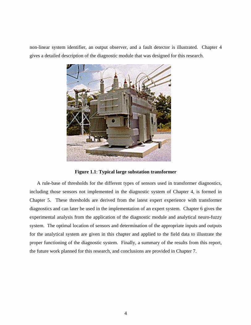
by the human operator, as might be the case with the knowledge-based approach as well. Figure

2.1 is a block diagram showing the steps that are taken for both the knowledge-based and

analytic model-based approaches.

Figure 2.1: Various approaches to fault diagnosis

15

2.2.2 Analytic Models for Transformer Diagnostics In the beginning, most attempts in transformer diagnostics focused on analytic models. As

mentioned in the previous section, analytic models attempt to represent the system through

mathematical equations. Depending on the complexity of the system and the desired model

accuracy, both linear and nonlinear models have been developed. These models attempt to use

physical principals to model a system. In the case of transformers, nonlinear models are needed

in order to describe the inherent complexities of the system.

Model-based monitoring of transformers was introduced by MIT researchers (Hagman, et.

al., 1996). It has subsequently been implemented on several transformers around the United

States. In this model-based monitoring, actual measurements are compared with predictions

based on operating conditions and ambient temperatures to provide a better assessment of the

actual transformer condition. A schematic of the idea behind model-based monitoring is given in

Figure 2.2. Parameter estimates for the model of the transformer system are calculated given a

set of inputs and outputs. Once the model is developed, residuals are generated between the

model outputs and the actual outputs. These residuals are put into an adaptive mechanism that

recalculates the system parameters. The parameter estimation allows the diagnostic system to

tune itself to each given transformer. Rapid deviation of model parameters indicates a

developing fault. Slow changes in the parameters may only signify a slow developing fault or

normal aging. Through trending of the parameter changes for a properly operating transformer,

it also becomes possible to make life expectancy predictions (Hagman, et al., 1996).

For transformers, many different types of models have been developed to try to identify the

system and detect failures. The transformer system is very complex. It contains thermal,

mechanical, electrical, and fluid systems. Though most effort was made at linear models of the

transformer systems, it quickly became evident that non-linear models provided for more

accurate system identification (Archer et al., 1994). Using these models, it has become possible

to detect faults by noticing abrupt and slowly developing changes in the model parameters. The

16

added complexity that non-linearity introduces to system modeling renders it impractical in most

cases.

Figure 2.2: Model-based monitoring scheme for transformer

The most common models that have been experimented with are thermal models. The IEEE

had developed a model for the top oil temperature rise above ambient temperature. As later

researchers found, the IEEE model did not accurately account for changes in the ambient

temperature that may occur. Subsequently, research was done at MIT to find a replacement for

the MIT model. They developed a top oil model that incorporated ambient temperature

variations to provide a system that was suitable for on-line monitoring and diagnostics (Lesieutre

et al., 1997). In addition, the system used top oil temperature measurements in coordination with

dissolved gas content to form an adaptive and intelligent monitoring system, utilizing thermal

modeling (Kirtley et al., 1996).

Much like the system developed at MIT, Ottele presented a thermal model of the transformer

using a physical based mathematical approach. An electrical circuit modeled the transformer,

where capacitors and resistors represented the different thermal masses and thermal

conductivities, respectively. The challenge was to determine the proper value for these critical

transformer parameters. Ottele used both a Hopfield based adaptive observer and a modified

17

extended Kalman filter to solve for the unknown states and parameters. The Hopfield network

would give the least squares solution, while the Kalman filter would give a linear approximation

based on Newton’s method. In both cases, the solution resulted in the values for the unknown

states and parameters of the system. Large state variations indicated failures or developing

failures (Ottele, 1999).

For protection against overloading, transformer thermal models have also been developed,

which use two exponential equations and non-linear time constants determined from transformer

data (Zocholl & Guzman, 1999). These models are used to predict top-oil rise over ambient

temperature, hottest-spot conductor over top-oil temperature, and hottest-spot winding

temperature given a specific load. This allows the utility to predict the damage that can be done

from running a transformer at a given load but also can be used to detect failures when there is a

discrepancy between predicted temperatures and the actual measured temperatures.

Many models have been formed that combine temperature measurements with current,

voltage, and other transformer measurements. Meliopoulos proposed a monitoring system that

would estimate the transformer hot spot temperature, the loss of life (LOL), and the transformer

coil integrity. State estimation methods were used, such as Cholesky factorization, to provide

accurate estimates using oil, tank, and ambient temperatures in addition to the voltages and

currents on all the phases as well as the LTC position (Meliopoulos, 2001).

In addition to the thermal models, many mechanical, electrical, and even fluid models have

been developed for the transformer. On the mechanical side, a mathematical model has been

derived to express the mechanical stresses due to forces on the transformer windings. This

model provides critical information on the possible damage that is caused from radial short-

circuit forces and gives an assessment of the possibility that a catastrophic fault from a winding

short circuit could occur (Weselucha, 1995). Likewise, diagnostics of the electrical system have

been developed using the transfer function method. Though the method uses ratios of the

transformers electrical voltages and currents, the method actually detects defects in the

mechanical system. The transfer function method is a quotient of the Fourier transformed input

and output signals. These quotients are used to model the system electrically, and through

18

comparison with previous fingerprints, can detect developing defects (Christian et al., 1999). In

addition to the mechanical and electrical modeling strategies, fluid models have been developed

for the transformer oil and its gas content. For bubbles to form, they must press against the

surrounding liquid (i.e. mineral oil). The formation of bubbles inside the transformer is critical

because the causes of bubbles are all linked to developing failures in the transformer.

Supersaturation of the oil by gas, decomposition of the cellulose insulation, and vaporization of

water in the oil all produce bubbles. The model indicates the temperature levels at which the

bubbles form and thus allows for warnings when the temperature reaches the levels indicated by

the model (McNutt et al., 1995). Finally, chemical models of the transformer insulation have

also been developed. The insulation model uses degree of polymerization and tensile strength of

the insulation to make fairly accurate estimations of the aging and life expectancy of the

insulation (Pansuwan et al., 2000).

The thermal models and many of the others given above are based in the time domain. In the

past few years, subspace-based identification of power transformer models have been formed

from frequency response data (Ackay et al., 1999). In this study, transformers are identified

through the use of a subspace-based algorithm in coordination with non-linear least squares

technique. The identified transformers have a dynamic range of 1 MHz and still produce

accurate models. In this method, mathematical frequency-based models are formed from which

equivalent circuits can be derived to match the frequency response of the model. The resulting

models are usually higher order but can be reduced through model reduction and still produce

highly accurate mathematical representations of the system.

2.2.3 Artificial Intelligence Diagnosis of Transformers There are several different techniques for fault detection and diagnostics. The knowledge

required for the fault detection engine varies greatly with the technique used. The modeling

techniques described above require significant knowledge about the system. The physics behind

the operation of the device (i.e the transformer) has to be derived. This type of modeling is

known as white box modeling. For the model to be successful, there must be information

19

available about the inner workings of the system. On the other side of the spectrum, there is

black box modeling. Black box modeling does not require knowledge of the inner workings of

the system. Artificial intelligence is the prime example of the black box model. The artificial

intelligence trains itself to the system and provides diagnostic information based on a set of

inputs and outputs. The actual mapping that the artificial intelligence develops or how this

relationship relates to any physical principles is usually not defined. For the user, the inner

working of the fault detector is not important, rather only the output of the fault detector is of

interest. Figure 2.3 illustrates the difference between white box and black box monitoring.

Figure 2.3: Comparison between white and black box diagnostics

As noted earlier, the non-linearity of transformers makes it exceedingly difficult to create

white box models that provide a high level of accuracy. In addition, the many subsystems

(thermal, mechanical, electrical, fluid) present in a transformer make the system modeling very

complex. It is not feasible to determine the physical principles that inter-relate the subsystems

and accurately formulate a model system. For this reason, black box modeling, centered around

various artificial intelligence techniques, have become more popular for transformer diagnostics

(Jota et al.,1998). In this case, the artificial intelligence can solely be used or a hybrid of

knowledge-based and artificial intelligence techniques can be used (gray box diagnosis).

The most common forms of artificial intelligence used for transformer diagnosis are neural

networks and fuzzy logic. Petri nets and genetic algorithms have also been tried but with less

20

success. An overview of some of the artificial intelligence techniques that have been developed

for transformer diagnostics is discussed below.

Due to the complexity of the numerous phenomena, it is difficult to formulate a precise

relationship relating the different contributing factors. This uncertainty naturally lends itself to

fuzzy set theory. For this reason, most black box and gray box diagnostic techniques have used

fuzzy logic to some extent. Xu et al. developed a transformer diagnostic system that utilized

both an expert system and a neural network to detect failures in a transformer. The knowledge of

the expert system has many uncertainties, and therefore fuzzy logic is employed. In this case,

the neural network employs sampled learning to complement the knowledge-based diagnosis of

the expert system. The two techniques are integrated by comparing the expert system conclusion

with the neural network reasoning using a consultative mechanism (Xu et al., 1997). A block

diagram for this type of hybrid system is given in Figure 2.4.

Figure 2.4: Strategy for combined fuzzy logic, expert system, and neural network

Much like Xu, Gao and Yan also developed a comprehensive system that included fuzzy logic,

expert system, and an artificial neural network to detect faults in the insulation system. In this

21

case, fuzzy logic is implemented in coordination with the neural network. The output of the

neural network is numerical values between 0 and 1, which are placed in membership functions

based on a set of fuzzy rules (Gao & Yan, 2002).

The combination of an expert system with neuro-fuzzy techniques is not the only diagnostic

tool used in transformer systems. An integration of an artificial neural network and an expert

system has been developed for power equipment diagnosis. The system uses the neural network

to form implicit diagnostic rules and has the added benefit of logic regression analysis for fault

location (Wang et al., 2000). In addition, work has been done in predicting the moisture content

in the transformer oil using a neuro-fuzzy system, similar to the one presented and tested later in

this thesis. This method trains the network to the moisture content and then compares expected

and predicted values of the moisture content to detect failures (Roizman & Davydov, 2000). The

strategy for this diagnostic system is given in Figure 2.5.

Though many methods have employed some combination of fuzzy logic, artificial neural

networks, and expert systems, this is not always the case. A highly accurate two-step artificial

neural network has been used for transformer fault diagnosis using dissolved gas data. In this

system, two neural networks are used. One is used to classify the major fault types, while the

other determines if the cellulose insulation is involved (Zhang et al., 1996). In addition, a DGA

based diagnostic system has been developed that employs a single neural network that is trained

with an improved back propagation algorithm utilizing data pre-treating for higher accuracy

(Yanming & Zhang, 2000).

Fuzzy logic has also been used to diagnose the health of a transformer and foresee any

developing failures. Fuzzy logic has been used to smooth out some of the problems that can

appear when using the cut and dry rules of expert system knowledge. By forming fuzzy

membership functions for the different measurements (gases, generation rates, electric current,

temperature), it is possible to overlap the individual membership functions into one large fuzzy

matrix that can be used for diagnosis (Denghua, 2000). A fuzzy logic diagnostic system has also

been developed for the transformer that utilizes evolutionary programming and different shaped

22

membership functions to get a more accurate fuzzy diagnostic system. This is formulated as a

mixed-integer combinatorial optimization problem (Huang et al., 1997).

Figure 2.5: Fault diagnosis method utilizing neural network on moisture data

Another artificial intelligence based approach utilizes a genetic algorithm in coordination

with an artificial neural network. One of the weaknesses of the artificial neural network

approach is the tendency to find only a local minimum in its training due to improper initial

value. In this case, the genetic algorithm is used to optimize the initial value and thus increase

the accuracy of the neural network training (Wen et al., 1997). Likewise, genetic algorithms

have been used in the training of a fuzzy controller that forms diagnostic rules based on

dissolved gas data. In this case, the fuzziness helps define diagnostic operating conditions and

the genetic algorithm decreases the amount of rules needed (Szczepaniak, 2001).

In addition to genetic algorithms, Petri nets have found some applications in transformer

diagnostics. The type of system affects how the Petri net operates and fails and what can be

diagnosed from the failure of the net. One method is to construct redundant Petri net

embeddings, which can then be used to identify place or transition failures. A transition failure

models a failure in the hardware performing a certain transition (in a discrete event system),

since no tokens are deposited to their appropriate output places or none are removed from the

input places. The first is a failure of the post conditions; the second is a failure of the

23

preconditions. A place failure, on the other hand, corrupts the number of tokens in a single place

(Hadjicostis, 2000). Coloured Petri net (CPN) models have the added benefit that the tokens are

distinguishable. These can be used even more effectively to diagnose a complex system. The

structure of the Petri net is a graph describing the structure of a discrete event system and the

dynamics of the system is described by the execution of the Petri net (Szucs et. al., 1998). The

Petri net in essence models the whole system, both the system states and error states. Once the

Petri net model is formed, a reachability tree starting from the initial state can be formed.

In Petri net diagnostic systems, predictive learning is also possible. In this case, the

diagnostic system archives all events measured online. If an unmodeled event or state occurs,

the Petri net adds the description to the system. It might be possible to apply these techniques to

transformer diagnostics. However, the transformers lack of discrete event makes the problem

more difficult. A fast and accurate transformer diagnostic system has been developed in China.

The Petri net operation matrix is used for knowledge representation and inference. From this

matrix, a relationship between the fault warning and the fault itself can be formulated (Wang and

Ji, 2002).

3. Neuro-fuzzy Fault Detection Engine In Chapter 2, many different diagnostic techniques were described. Analytical models can be

used to describe dynamics of the transformer system. However, it can be realized that modeling

of the entire transformer system, in order to accurately diagnose failures, is not feasible. For this

reason, artificial intelligent techniques are employed to detect developing faults in transformers.

As described in Chapter 2, the combination of neural networks and fuzzy logic is common in

transformer diagnostic systems. The neuro-fuzzy engine proposed in this thesis utilizes neural

network and fuzzy logic for the purpose of non-linear system identification, output observation,

and fault detection. This neuro-fuzzy system has been implemented and tested by the research

team in their prior investigation related to the development of an Intelligent Substation, and has

24

been found to successfully detect failures in such non-linear thermofluid systems as refrigerators

and distribution transformers.

The description of the neuro-fuzzy system used in this research is given below. A

mathematical description of the inner workings of the system and how the final fault detection

decision is made is also described. The work described here is part of the effort of the research

team headed by Dr. Shoureshi and his graduate students, Hu (2000) and Fretheim (2000).

3.1 Overview of Diagnostic Approach

The diagnostic approach developed by the research team can be divided into several parts.

First, relevant, diagnostic data must be collected from sensors. From this set of data,

measurements are chosen to be either inputs or outputs. The neuro-fuzzy network then receives

the data and performs several tasks. Non-linear system identification is the first step performed

by the network. Through training, the neuro-fuzzy network identifies the non-linear system

dynamics, so that future estimations can be made. Once trained, the network can serve as an

output observer. The trained network processes data and estimates the output. These estimates

can then be compared to the measured outputs to form residuals. The final step is to analyze the

residuals produced by the neural network in order to detect faults. The assessment of the

transformer health and any need for maintenance can be established. A block diagram of this

approach is shown in Figure 3.1.

25

Figure 3.1: Block diagram of diagnostic approach

The following sections describe the architecture of the neuro-fuzzy network used in the research

and give the mathematical foundation for the non-linear system identification, output

observation, and fault detection.

3.2 Non-linear System Identification This section focuses on the theoretical basis for non-linear system identification, which is

applied to the transformer. The purpose of system identification is rather simple. Through

observing the system, a model is formed that attempts to duplicate the behavior of the system.

As the size and complexity of the system increases, it becomes more difficult to develop

26

analytical models. The more accurate the model the smaller the error will be between the model

estimates and the actual outputs. A block diagram of the operation of a system identification

technique is depicted in Figure 3.2.

Figure 3.2: Process of system identification

In the case of the transformer, simple analytical models often cannot accurately portray its

dynamics. Therefore, neural networks are commonly used for non-linear system identification of

transformers. A summary of previous research related to non-linear system identification using

neural networks is discussed below.

3.2.1 Background of Neural Networks for System Identification As mentioned in Chapter 2, one alternative to complex analytical modeling is system

identification through other means, such as artificial intelligence (Ljung, 1999). In more general

terms, system identification is the name given to the various methods which use input output data

to develop dynamic models for a system.

Until about the mid-1980s, non-linear models of systems were primarily derived empirically

or from first principles. If these analytic models were too complex to derive, a linear

approximation could be made through input output data, or nonlinear systems could be linearized

around an operating point. For example, the extended Kalman filter uses a linearization around a

certain point to try to approximate the non-linear behavior. By applying techniques based on

complex variables, linear algebra, and ordinary differential equations, complex systems could be

identified.

27

Despite the growing expertise and experience that had been formed in the area of linear

system theory, non-linear system identification was still a relatively new topic. Few people had

focused their attention on non-linear system identification. In the case of non-linear systems,

stability, system behavior, and robustness had to be analyzed differently for each case. There

were no general rules that could be applied as in the case of linear systems. In the 1980’s with

the introduction of neural networks, non-linear system identification received much more

attention. A neural network is meant to operate like a human brain. Just as the human mind

makes decisions based on past learning experiences, a neural network produces outputs by

processing a set of inputs based on past learning. Narendra and Parthasarathy (1990) published

the first, feasible neural-based method for non-linear system identification. Two categories of

neural networks have been considered for this application: 1) multilayer neural networks and 2)

recurrent networks. Multilayer neural networks represent static non-linear maps, while recurrent

networks represent non-linear dynamic feedback systems. Using back propagation techniques for

training, non-linear system identification was found to be feasible through neural networks.

Neural networks were first used to identify process dynamics in nuclear power plant

components (Parlos and Atiya, 1991; Parlos et al., 1994). A recurrent multilayer perceptron

network is used, where the architecture is a mix between feedforward and feedback. In the

nuclear power plant case, the network is compared to an analytic white box model derived from

physical principles. The results of the neural network compared well with the analytic model

and showed that for this specific application, neural networks can succeed in non-linear system

identification. Though it is not clear whether the recurrent feature in the neural network

improved the results, most subsequent research is aimed at these recurrent networks.

Qin and McAvoy (1992) compare recurrent networks versus feedforward networks and batch

learning versus pattern learning. Four neural network learning algorithms are used in their

experiments. The results show that the recurrent network is more robust to noise but has a more

complicated training routine. The same experimental result is achieved by an independent

experiment (Nerrand et al., 1994), where a discussion of training recurrent neural networks for

process modeling is described. The ultimate decision on the type of training that should be

28

employed for non-linear system identification should be based on the noise involved in the

process. Batch learning is appropriate for white noise or noiseless systems.

For systems where the noise varies or is not deterministic, many different methods have been

developed for training. Das and Olurotimi (1998a; 1998b) discuss how to train recurrent neural

networks with noise present. There are many different architectures and training algorithms to

choose from and careful effort should be taken in picking the algorithm appropriate for the

system at hand.

The question is often posed as to whether a recurrent network is worth the added complexity.

A recurrent network does add many more connections than a feedforward/feedback architecture.

It has been proven that a recurrent network can serve as a universal approximator of an arbitrary

non-linear mapping, provided a few conditions are met, whereas the same cannot be said of the

feedforward/feedback networks (Chen and Chen, 1995).

The training algorithm of both multi-layer feedforward neural networks (MNN) and recurrent

neural networks (RNN) are usually based on a back propagation (BP) algorithm, as were the first

neural networks used for non-linear system identification (Rummelhart et al., 1986). The BP

algorithm for MNN’s are better understood than RNN’s (Das and Olurotimi, 1998a). As such,

there has been much more success in using MNN’s for non-linear system identification, pattern

recognition, controls, and signal processing than there has been using RNN’s. Over the years,

many improvements have been made on the standard BP algorithm, such that it would have a

faster convergence. Despite the improvements, the major disadvantage of BP based neural

networks is the slow convergence and the susceptibility to falling in a local minimum.

In order to try to compensate for the problem of slow training, radial basis function neural

networks (RBFNN’s) (V.T. and Shin, 1994), which can approximate any static non-linear

function to some desired accuracy (Haykin, 1994), was introduced. In most cases, the RBFNN

has faster training, since it does not use a BP algorithm. However, the training can often result in

an ill-conditioned least mean squared (LMS) problem. In addition, the memory requirements can

get extremely large when dealing with larger data sets. In general, RBFNN has two major

disadvantages: computational complexity, and lack of spatial varying resolution (Suykens and

29

Vandewalle, 1998). Despite these problems, RBFNN has been found to be effective for non-

linear system identification as discussed by Juditsky et al. (1995).

The above forms of non-linear system identification only use neural network architectures.

As noted in Chapter 2, it has become common to incorporate fuzzy logic with neural networks.

Much like neural networks, fuzzy logic can also be used to form models for non-linear systems

based on input output data (Suykens and Vandewalle, 1998). A structure that holds increased

potential for fuzzy modeling is the Takagi-Sugeno (TG) system. This system combines an

artificial neural network with fuzzy logic to create a neuro-fuzzy system for non-linear system

identification. This hybrid system is known as a Tsukamoto-Type Neural Fuzzy Inference

Network (TNFIN), which is an extension to the TS fuzzy system (Hu et al., 2000). It is this

form of black box modeling that is used in the present research for system identification and fault

detection. This technique displays a fast and accurate training and has compared well with the

MNN’s and RBFNN’s in previous studies (Fretheim, 2000).

3.2.2 Neural Network Architectures As shown in the preceding section, there are many different types of neural network

architectures that can be used for non-linear system identification. They all have their strengths

and weaknesses. When choosing the appropriate algorithm, there are two properties that are

crucial. First, the training algorithm should be fast and the parameters space must not be too

large that the architecture cannot be implemented in a real-time scenario. Fretheim (2000) did a

study of the different types of neural network architectures, including MLPNN, RBFNN, and

TNFIN. Through experimental studies with a refrigerator diagnostics and distribution

transformer systems, it was found the MLPNN is well understood but has the tendency to fall

into local minima. The RBFNN performed comparatively with the TNFIN with respect to

accuracy. However, the RBFNN requires nearly three times as many parameters as the TNFIN.

This is computationally expensive and undesirable for the purposes of non-linear system

identification for the transformer. Due to the results with the small distribution transformer, the

TNFIN is used for this research, where a larger transformer is being identified.

30

The TNFIN was developed and first implemented by Zhi Hu (2000). The TNFIN was

originally implemented as a load forecaster but was later applied to non-linear system

identification (Fretheim, 2000). Experience with non-linear systems has shown that the TNFIN

does not have the tendency to fall into local minima as is the case for the MLPNN. The training

algorithm for the TNFIN has also been improved to make it comparable with the RBFNN. With

this fast training capability of the TNFIN, non-linear system identification became possible. To

better understand the TNFIN architecture and how it can be used for system identification, an

overview of the TNFIN is given below.

3.2.3 TNFIN Architecture

TNFIN is a multi-layer feedforward neural network. The number of layers in the TNFIN is

held constant at 4. The TNFIN can handle any number of inputs and outputs, which makes it

applicable for many different systems. The architecture used in this research is a slight variation

of the original network presented by Hu et al. (2000), which had five layers.

A schematic of the general architecture of the TNFIN is presented in Figure 3.3. The figure is

shown for the case of two inputs and two outputs. The network can be adjusted for any number

of inputs and outputs. The equations and constraints given below are for the two input, two

output case. The parameters that are adapted during training show up in the functions of layers 1

and 3.

Layer 1: This is the fuzzification layer. Each node of the first layer gives a membership degree

of a linguistic value. For a network with N inputs, the first layer places each input into a fuzzy

set. The total number of nodes in this layer is equal to the number of inputs (N) times the

number of membership functions in the fuzzy set. The kth node in this layer performs the

following operation:

)(1iAk xO

ijµ= (3.1)

where

jik +−= )1(*2 )21,21( ≤≤≤≤ ji

31

ix is the ith input variable, and is the jth linguistic value associated with the input ijA

variable . Thus, denotes a membership function related to and specifies the degree of

belonging to .

ix1kO ix ix

ijAijAµ is chosen as a bell-shaped function without an exponential parameter.

There must be at least as many membership functions as there are inputs to the TNFIN.

Figure 3.3: Architecture of the TNFIN

32

Once the number of membership functions has been decided for layer 1, the network structure

for all the remaining layers is established as well, and layer 1 becomes:

])[(1

1)(2

1

ij

ijiiAk

baxxO

ij −+

== µ (3.2)

where

jik +−= )1(*2 )21,21( ≤≤≤≤ ji

and the set of parameters associated with the jth membership function of the ith input

variable is referred to as antecedent parameters and is used to adjust the shape of the membership

functions in layer 1. Since there is both a and b parameters, the number of adjustable parameters

is twice the number of membership functions.

, ijij ba

Layer 2: Layer 2 serves as the normalization layer. The weighted outputs from the nodes of

layer 1 are normalized. The total number of nodes in layer 2 is equal to the number of nodes in

layer 1. The output is simply given by:

1

12

kk

kk O

OO

Σ= )21( Nk ≤≤ (3.3)

Layer 3: Once the inputs have been fuzzified and normalized, they must once again be

defuzzified. Therefore, layer 3 serves as the defuzzification layer. The total number of nodes in

this layer is equal to the number of nodes in layer 1 times the number of outputs. Each node

from Layer 2 expand into two (number of outputs) same type nodes in layer 3, which contain two

types of functions, either a monotonically increasing or monotonically decreasing function.

Tsukamoto-type fuzzy reasoning (Tsukamoto, 1979) is used for fuzzification.

Thus, the defuzzified values for the output of this layer are specified as follows:

33

⎪⎪

⎩

⎪⎪

⎨

⎧

=−+

=−−

=

even k if)11(

odd k if)11(

22

22

3

kklklk

kklklk

m

OdcO

OdcO

O (3.4)

where

2) l 1 4, k (1 1 1)-(k * 2 m ≤≤≤≤+=

Layer 4: The fourth and final layer in the network architecture is the summation layer. It sums

the outputs of layer three together into an output. There are as many nodes in this layer as there

are outputs. There is only one connection between each node in layer 3 and a node in the output

layer. The output of this layer is simply:

(3.5) ∑ +−=k

lkl OO 3)1*(2

4

3.2.4 Hybrid Learning Algorithm

Training of the TNFIN network is done with a hybrid learning algorithm that incorporates

both error minimization and supervised learning. Hu (2000) provides a detailed description of

the training algorithm used for the TNFIN. A few of the unique parts of the training algorithm

are discussed here.

As noted above, the training of the network is done using supervised learning and error

minimization. When p is the number of training sets and l is the number of inputs, training is

performed by:

24,

*,,

24,

*,

)(21

)(21min

lplplp

plp

llp

OTEand

OTE

−=

−= ∑∑ (3.6)

34

where E is the mean squared error between the training and the output, O4p,l is the lth output of

the network for the pth training set, and T*p,l is the measured target.

The parameters c, d in layer three are updated using a LMS algorithm. The following steps

are performed during each complete iteration of the TNFIN training algorithm:

Step 0:

Initialize parameters a, b to a predefined value, and set parameters c, d equal to zero.

Step 1:

Calculate the consequent parameters c, d using LMS algorithm.

Step 2:

Calculate a range of learning rates to use.

Step 3:

Use GD (gradient descent) algorithm to minimize the output with respect to a, b, followed by

LMS algorithm to calculate the respective c, d. For all the learning rates calculated in step 2,

repeat starting from the minimum after step 1.

Step 4:

The final parameters to be used for the network are chosen from the minimum of step 3. If the

value is not small enough, further training may be done by repeating steps 2 and 3.

Due to the linear relationship between the parameters in layer three and the error E, the

training of the consequent parameters through the LMS algorithm is fast. In addition,

the GD approach, that adjusts the antecedent parameters with different learning rates from the

same starting point, helps to avoid falling into a local minima.

Training of this network was used for a small 10kVA transformer that was anticipated to

simulate a larger transformer, similar to the ones used in this research (Fretheim, 2000). It was

found that large data sets were necessary to capture the full dynamics of the transformer system.

When these larger sets of input output data were used, the TNFIN trained quickly and with a

small error of less than .05 (normalized). It is found that the problems of slow convergence and

local minima were avoided. With the positive results from the small transformer already

35

documented, it was the natural choice to use the TNFIN for system identification on the larger

transformers used in the present research.

3.3 Neural-Based Non-linear Observer In addition to system identification, the neural network will also serve as an output observer.

This observer problem can be defined as a solution to a set of non-linear equations, and solved

using non-linear least mean squares (LMS), the same method used in the training of the neural

network. Newton’s algorithm and Levenberg-Marquardt’s method, two well known LMS

techniques, are considered. This neural-based observer will serve as the foundation for the fault

detection approach of the next section.

3.3.1 Observer Introduction and Background The goal of an observer is to provide an estimate of the state of a dynamic system using only

input output data. Work in attempting to find the solution to a state estimator for a linear, time

invariant system first began in the mid 1960s (Luenberger, 1963). To understand the

mathematical basis of an observer, first consider the n-dimensional linear time invariant system:

)()1()1()1()1(

kCxkykBukAxkx

=++++=+

(3.7)

where A,B, and C are respectively n × n , n × p , and q × n matrixes, is the state

vector, is the system input, and is the system output. If we are given the

measurements [y(k) y(k -1) · · · y(k -l)], and the inputs

nRkx ∈)(pRku ∈)( qRky ∈)(

[u(k) u(k - 1) · · · u(k - l)], the problem for the observer is to find an estimate of the state

trajectory , where indicates an estimate of the true )]()1(),([ lkxkxkx −−∧∧∧

L (.)∧

x

states x(·).

36

After success of observer designs with linear, time invariant systems, widespread work has

been devoted to expand the observer design to time-varying linear systems, and to non-linear

systems. Due to their lesser amount of complexity, most effort has focused on linearizable

systems (Baumann and Rugh, 1986). Stable observers have also been developed using quadratic

Lyaponov functions (Thau, 1973). In addition, there has also been some success using Hopfield

neural networks for state observers (Chu et al., 1989; Chu and Shoureshi, 1994). Likewise,

Kalman-type and Luenberger observers have also been extended to incorporate the non-linear

systems in continuous time (Gauthier et al., 1993; Deza et al., 1992).

Non-linear observer design is still an active research topic. Methods are currently being

developed to try to apply to broad classes of non-linear systems. Michalska and Mayne (1995)

have proposed an optimized moving horizon observer, while Grizzle and Moraal (1995) derived

an approach to solving systems of non-linear equations applicable to a wider class of non-linear

observer design. The observer problem can also be analyzed by solving a set of differential

algebraic equations (Nikoukhah, 1998).

In finding an observer, it is not always necessary to have a system model, as utilized in the

case of linear observers. Using a neural network to train itself to estimate the states from input

output data, it is possible to create an observer that uses only input data (Levin and Narendra,

1996). For this to work, however, the dynamic system trajectory must be limited. This is

feasible for control systems where one knows the outputs and inputs that are available.

For the purposes of diagnostics, state observers may also be used. Observers used for fault

detection are quite similar to those used for state estimations. The main difference is there is no

need for a comprehensive knowledge of the state space in diagnostic applications of observers.

For diagnostics, an output observer is used to help determine changing relationships between

signals so that an output value may be estimated. This estimated value can then be used to

determine any developing abnormalities or dramatic changes in the system.

In fault detection, the difficulty is associated with determining which sensor measurements to

use as inputs and outputs of the system. In the case of the diagnostic module designed in this

research, the current, temperature, and vibration data must be used to train the network. The goal

37

is to choose inputs and outputs chosen that would cover the range of normal operating

conditions. The key for fault detection is that the observer be able to detect changing dynamics.

In this section, a new analytic technique for output observer design for non-linear systems is

described where the intended application is fault detection. Instead of identifying the inverse

mapping directly, a neural network will be used to determine the forward dynamics of the

system. The observer then uses the identified model to estimate unknown outputs from known

outputs and inputs. The neural network is only used to represent the system dynamics and thus

the observer can be used to solve for different outputs depending on the available inputs. The

inputs and outputs to the observer are not fixed and, therefore, there is a greater flexibility.

Later in this chapter, it will be shown that this flexibility is a requirement for a new fault

detection approach. The TNFIN network discussed earlier is used to model the system.

However, any neural network architecture can be used for the observer design that is described

below.

3.3.2 Nonlinear Observer Using Neural Network Dynamic Models

The class of systems to be considered can be described by:

))(),(()(

))(),(()1(kukxgky

kukxfkx=

=+

where x ∈ Rn, u ∈ Rm, y ∈ Rp.

An alternative representation for the system is as a predictor equation of the following form:

),...,,,,...,,(

)1(......

)1()1(

2121

2

1

mp

n

uuuyyyF

ky

kyky

=

⎥⎥⎥⎥⎥⎥

⎦

⎤

⎢⎢⎢⎢⎢⎢

⎣

⎡

+

++

(3.8)

38

where:

)(),...,1(),(

)(),...,1(),(

ilkukukuu

jlkykykyy

iiij

jjjj

−−=

−−=∆

∆

The model representation given by (3.8) has been discussed in (Shoureshi et al., 2000). The

identification of a non-linear system involves training the neural network to approximate the

mapping described by equation (3.8). The spaces defining the input and output sequences of the

system are represented by U ∈ Rr, Y ∈ Rp, and Yin ∈ Rq, where

⎟⎟⎠

⎞⎜⎜⎝

⎛=

⎟⎟⎠

⎞⎜⎜⎝

⎛=

−−−−−−=

=

−−

−−−−=

∆

∆

∆

∆

∆

in

delayin

Tppdelay

Tp

Tmmm

YU

Z

kYkY

kY

plkykylkykylkykykY

kykykykY

mlkukuku

lkukukulkukukukU

)()(

)(

)](),...,1(),...,2(),...,1(),1(),...,1([)(

)](),...,(),([)(

)](),...,1(),(

),...,2(),...,1(),(),1(),...,1(),([)(

2211

21

222111

Let be a neural network representing the mapping given by Equation (3.8). pqrf RZNN →+:

Let )())1(),1((: lkYlkUlkYNN infl +→−+−+

Let one output be measurable for all time k. iy

Let where and ]1[ pC ×=∆

1=iC 0=jC where ij ≠

A sequence of l observations can be described by the following set of equations:

39

(3.9)

⎥⎥⎥⎥⎥⎥

⎦

⎤

⎢⎢⎢⎢⎢⎢

⎣

⎡

−+−+∗=+

++∗=+∗=+

))1(),1(()(......

))1(),1(()2())(),(()1(

2

1

lkUlkYNNClky

kUkYNNCkykUkYNNCky

infli

infi

infi

where the term selects out only the measurable output, which will later be compared with

the actual output in the LMS algorithm.

*C

Due to the forward prediction of the , the only unknown in equation (3.9) is the vector

. If there exists a unique solution to this set of equations for some value of l, it is stated

that the system is output observable, and the vector can be recovered through a non-linear

LMS algorithm.

fNN

)(kYin

)(kYin

The existence of the solution to Equation (3.9) is guaranteed if the output observability

condition is satisfied. For a non-linear system, the concept of output observability becomes a

function of the system trajectory, and hence, the existence of a solution to Equation (3.9) changes

with time. Even if a solution exists, finding the inverse of the non-linear LMS problem can in

many cases result in an ill conditioned solution. This is undesirable because any small

disturbances or modeling errors can create large changes in the estimation of the unknown

outputs.

An alternative approach to the non-linear neural network observer is to directly identify the

inverse mapping using an artificial neural network (Shoureshi et al., 2001). The disadvantage of

this approach is that all physical insight into the system dynamics is lost. Through identifying

the system, any output can be considered the known measurement. This is extremely helpful in

fault detection, where the dynamic model is used as a basis for fault detection.

40

3.3.2.1 Newton’s Method

Newton’s method (Shoureshi et al., 2001) was implemented to solve the set of Equation (3.9)

as a root finding problem, and was implemented on a system with very little noise, and small

modeling errors.

The algorithm converged quickly and reached a solution by selecting the best estimate of the

output value and updating the value according to a standard algorithm.

In reality, the algorithm is terminated when the solution converges, or a fixed number of

iterations have passed and the solution is not found. When no noise is present and the system

has been accurately modeled, the algorithm worked suitably. However, noise in the system, or a

poor initial guess had a tendency to make the algorithm diverge. The Levenberg-Marquard

algorithm is found to be a more robust solution to the problem.

3.3.2.2 Levenberg-Marquardt Method

As a general nonlinear least squares equation solver, the Levenberg-Marquard algorithm

(Shoureshi et al., 2001) has demonstrated good performance. The algorithm will always take a

step in a descent direction and will not diverge as in the case of Newton’s method when noise

was present. The challenge is estimating a good initial state, when an acceptable local minimum

or global minimum is desired. To be preferable over Newton’s method, the observer must

converge even in the presence of noise. By solving Equation (3.9) without regularization and

then adding a regularization term, the observer becomes more robust in the presence of

disturbances.

Let

Tinfmminfinfin UYNNCyUYNNCyUYNNCyYR )],ˆ(),...,,ˆ(),,ˆ([)ˆ( 2211 ∗−∗−∗−= ∗∗∗

∆

minimize ∑=

==m

iiniin

Tinin YrYRYRYf

1

2)ˆ(21)ˆ()ˆ(

21)ˆ( (3.10)

41

where is nonlinear in and )ˆ(, inYRqm > inY

qin RY ∈ˆ

),ˆ()ˆ( UYNNCyYr infiiini ∗−= ∗

where is the observed value and is estimated by the model. ∗iy ),ˆ( UYNN infi

If a solution exists, the global minimum = 0. However, modeling errors and noisy

measurements will often result in a solution greater than 0. Let be the estimate of as a

starting point. The recursive update of then becomes:

inY )(kYin

inY

)ˆ()ˆ(])ˆ()ˆ([ˆˆ 1in

Tincin

Tinin YRYJIYJYJYY −

+ +−= µ (3.11)

where 0=cµ if and 21 ||)ˆ()ˆ())ˆ()ˆ((|| in

Tinin

Tinc YRYJYJYJ −≥δ 0>cµ otherwise.

Here, cδ can change from one iteration to another, and will adjust the step size, , for

the next iteration. The solution to the minimization problem (3.10) represents the following

mapping:

+= YYinˆˆ

)()](),...,1(),(),(),...,2(),1([ kYlkUkUkUlkykyky inlii →+++++ ∗∗∗ (3.12)

When there are noisy conditions present and the solution is poorly output observable, small

deviations in can cause large deviations in the estimate of . ∗iy inY

It is possible to stabilize the solution even around poorly observable regions by adding a

regularization term:

Let where and ]1[ pD ×=∆

0=iD 1=jD where ij ≠ ,

42

and i is the measured output

Let ))1(),1((ˆ1 −−∗=

∆∗∗ kUkYNNDY inf

Let , where α is a weighting factor. )ˆ)(ˆ())(ˆ( ∗∗∆

−= YkYkYG inin α

Here, ) represents the regularization term. Now, the minimization problem )(ˆ( kYG in

becomes:

)])ˆ(),ˆ([)]ˆ(),ˆ(([minimize2

)( ininininin YGYRYGYRYf = (3.13)

The observer problem with an inverse mapping now becomes a forward predictor by adding

n term. When the observer problem is ill-conditioned (i.e he Jacobian of

)ˆ()ˆ( inT

in YRYR is not full rank or poorly conditioned), there are some terms of inY that don’t have

a unique solution or are sensitive to noise in the data. When this problem occurs, the

regularization term becomes dominant in the minimization alg

1ˆ T

a regularizatio . t

orithm for the terms of that are

ausing problems, and the forward prediction is used instead.

tecting abnormalities in a

on-linear system. The benefits of this approach are described below.

inY

c

3.4 Fault Detection In section 3.2, it was described how the TNFIN neural network can be used to identify a non-

linear system, in the case of this research a transformer. The system is identified using just

inputs and outputs to the system. In the previous section, the analytic background for a neural

based observer was discussed. Once again, the TNFIN architecture was used by the observer to

produce output estimates. From this observer design, a new fault detection approach can now be

utilized. This new fault detection approach for non-linear systems is discussed in this section.

The result of the new approach is a practical and general method of de

n

43

3.4.1 Background of Fault Detection Approaches

For fault detection to occur, there must be the presence of constraints or redundancies that

define normal operating conditions. In the analytic methods of redundancies, an observer, which

contains a model of the system, is used to generate a residual. This residual is the difference

between the observer estimate and the actual output, as given by some sensor measurement. In

the ideal case, a non-fault condition would be indicated by a residual that is zero, while the

presence of a non-zero residual would indicate a fault. However, the model of the system is not

perfect, and as such, there will be some uncertainties present that will cause a residual to exist

even under normal operating conditions. For this reason, some accommodations must be made

and boundaries must be set for determining normal operating conditions. Many robust fault

diagnostic methods have centered around this topic. Some have attempted to represent both the

faults and model uncertainty as inputs and then try to decouple the residuals produced by faults

and those produced by uncertainties in the model. In other approaches, the probability of a given

set of outputs actually being produced by a system given knowledge about the noise,

disturbances, and model error is determined. If the probability shows the data set is highly

unlikely, the model is invalidated. If the model is representative of a normally operating system,

then a fault has occurred when the residual becomes larger.

Using the results that have been achieved, based on the TNFIN, to identify and observe a

small scale (10kVA) transformer system, a different approach can be derived for robust fault

detection using neural networks (Fretheim, 2000). This fault detection method can be applied to

a wide variety of non-linear systems. Work has been done in the past using neural networks for

fault detection. In most of these scenarios though, the neural network is used for pattern

recognition (Ficola et al., 1997). For this type of fault detection, the measured system outputs are

actually the inputs to the neural network, and the fault classification or fault parameters are the

outputs. In other schemes, neural networks are used to implement an observer that changes the

parameters to approximate the maximum likelihood estimate (Alessandri and Parisini, 1997).

Neural networks have even been applied to observers that can solve for inputs and predict

forward (Krishnaswami et. al., 1994). The fault detection method proposed here uses the neural

44

network for the purposes of modeling the dynamics of the transformer. A dead-beat observer is

then implemented by solving a set of non-linear equations. Using this method, it becomes

possible to introduce constraints into the system, which can improve the accuracy of the fault

detection.

3.4.2 Observer Residual Generation

The observer design from Section 3.2 can now be used for generating residuals. By using

this observer, a fault detection approach can be implemented. The details of this approach are

given below. Figure 3.4 shows a simple block diagram for the implementation of the output

observer. One should notice that there are two residuals in the diagram: )(1 kε is due to the

uncertainty in the observer model, while )(2 kε is the difference between the estimated output and

the actual output. For the purposes of the transformer fault detection, the output observer must

be implemented on-line. For this implementation, the following are defined as: ∆

=)(ku system input(s)

∆

=)(* ky measured output, and input to observer

∆

=)(* ky any measured output, could be equal )(* ky but does not have to be.

∆

=)(ˆ * ky l Observer estimate of )( nkyl −

The term is shifted since in the real time scenario past values of the outputs are

being calculated.

)(ˆ nkyl −

45

Figure 3.4: Block diagram for on-line observer with residual generation

There are two different ways to detect changes in the system dynamics.

||))(),1(()(||min)( 1)(1 kynkuFkYkresidual lnln

kyl

−+−= −+

∆

ε (3.14)

)()(ˆ)( *2 kykykresidual −=

∆

ε (3.15)

Residual )(1 kε is the minimum achieved through training of the neural network. A large

value indicates that an accurate value of could not be determined by the observer.

Therefore, the observed outputs have difficulty in identifying dynamics of the system. This

residual can be used to measure whether if there is a significant change in the dynamics. Output

observability, noise and disturbances in the system, modeling errors also can contribute to the

size of

)(kyl

)(1 kε . Residual )(2 kε is a measurement of the difference between measured and

estimated values produced by the observer.

To understand the observability property of the system, consider two different functions, f1

and f2. These two functions both minimize the first equation in (3.14), but occur on different

points on the system trajectory. The system of f1 is poorly observable, while system f2 at the

current trajectory is considerably more observable. As illustrated by Figure 3.5, the minimum

of f2 is much more pronounced than the minimum of f1. The two residuals, )(1 kε and )(2 kε ,

respond differently to a poorly observable system.

46

For a poorly observable system, small changes in the data can cause large changes in

, but the error

*y

)(ˆ kyl )(1 kε will not increase significantly. Thus, )(1 kε is robust in regards to

disturbances in . With this advantage, there is also the disadvantage that )(ˆ kyl )(1 kε is not as

sensitive to changes in system dynamics. The exact opposite is true for the residual, )(2 kε .

Small changes in data can cause large changes in . A small change in the data can

cause relatively large

*y )(ˆ kyl

)(2 kε . In either case, the ability to use either residual )(1 kε or

residual )(2 kε to detect a fault is decreased as the system becomes less observable. For poorly

observable systems, )(1 kε might not detect a real fault, where )(2 kε could produce a false alarm.

Due to this fact, the fault detection approach used in this research combines the properties of

both the residuals to be able to increase sensitivity and robustness. The following section

describes the approach used for this research.

Figure 3.5: Comparison for degrees of observability

3.4.3 Optimization Based Fault Detection Approach Since a solution to the minimization problem of Equation (3.14) has already been

determined, the algorithm can be adjusted by taking into account previously known information,

such as available measurements, noise level of the sensors used, parameter bounds, etc. By

47

using this additional information, the reliability of the fault detection approach, as well as its

applicability to other systems, is greatly enhanced.

Equation (3.14) is a solution to a deadbeat observer problem. As noted earlier, ideally (i.e.

neural network mapping is an accurate representation of a system and there is no noise or

disturbances present), a no-fault condition would exist when the solution to Equation (3.14) is

equal to zero. In reality, there is inevitably going to be modeling errors, noise, and disturbances.

Therefore, the solution to the minimization problem of Equation (3.14) will never be zero.

Modifications must then be made to incorporate the uncertainties in the system. Thus, a no-fault

condition can be said to exist when:

ε<−+− −+ Wlnlnn

kykynkuFkY

l

||))(),1(()(||min 1)( (3.16)

where Wxxx W '|||| = . The goal now becomes to identify appropriate values for the parameters

W and ε . For this purpose, a data set different from the data used for the system identification is

used to represent the normal system behavior. Here W is a weighting matrix for x, and ε is set

as an upper bound on the error during a no fault operation. In this way, W can weight the more

important outputs. If the minimum of the solution to Equation (3.16) is less ε , there is strong

evidence that the system is operating normally. Information about the type of sensor

measurements used can determine an appropriate W. If the level of noise and the scaling of the

data is approximately the same, then an identity matrix may be used for W. For example, if the

scaling is different from one measurement to another, then W can be used to compensate for this

effect in the minimization of Equation (3.16). When an identity matrix is used for W, it is

assumed that the measurements are independent; hence, the non-diagonal terms are zero. There

could be cases that correlation may exist between different sensor measurements, which would

result in off diagonal terms in the matrix W. However, trying to determine the value of these

terms can be extremely difficult, especially for non-linear systems.

48

A new output sequence can now be tested for possible faults by determining if Equation

(3.16) is satisfied for the chosen values of W and ε . and )(),( kykY ln )1(1 −+−+ nku nl in

Equation (3.16) are now based on values from the data sequence to be tested. If the minimum is

less than ε , there is strong evidence of a no fault condition.

The minimization problem described by Equation (3.16) is generally exceedingly flexible.

Not all the terms in need to be used, nor do all terms in )(kY n )1(1 −+−+ nku nl , need to be

unknown.

)(kyl

Given a vector x of length r, and a finite set of integers M = i1, i2, i3, · · · , , si

rik ≤ and k = 1, 2, 3, · · · , s, let be the projection operator such that Mp

⎥⎥⎥⎥⎥⎥

⎦

⎤

⎢⎢⎢⎢⎢⎢

⎣

⎡

=

is

i

i

i

M

x

xxx

xpM

3

2

1

*

From , another projection operator can be defined as: Mp

⎥⎥⎥⎥

⎦

⎤

⎢⎢⎢⎢

⎣

⎡

=∆

M

M

M

zM

p

pp

L

M

L

L

00

000

π

where is a diagonal matrix of size [(r*z)×(r* z)]. For a collection of several measurements of

x, where = [x(k) x(k -

1) · · ·x(k - z)], then

zMπ

zx

)]'()()()()1(

)1()1()1()()()()([)(*

321

321321

zkxzkxzkxzkxkx

kxkxkxkxkxkxkxkx

isiiiis

iiiisiiizzM

−−−−−

−−−=

LL

LLπ

49

Using this operator, it is possible to select particular inputs or outputs from the vectors

or , etc. )1(1 −+−+ nku nl )(kyl

The minimization for fault detection now becomes:

Wlnlnn

Inn

Iyu

kynkuFkYl

yUnl

uU

||))(),1(()(||min 1,1

−+− −+−+ππ

ππ (3.17)

Through this procedure, a subset of the prediction equations in the set l is chosen for

evaluation. Meanwhile, the variables that are “known” in index sets Ku and Ky are fixed and the

variables that are unknown in sets Uu and Uy are calculated. Some of the variables collected in

or may be inputs, which are known, or outputs for which measurements

are (or are almost) noise free. When trying to detect faults, it may be necessary to test for sensor

failures by removing the data from a particular sensor. This fault detection approach easily

allows for identification of sensor failures.

)1(1 −+−+ nku nl )(kyl

Additional information may also be available about and ,

even if accurate measurements are not available. For example, the sensors may have a known

noise level with a magnitude bound of η, or there may be some bounds on the acceptable values

for other variables. This information can be expressed as a known set , for which the

unknown variables are known to lie:

)1(11 −+−+−+ nku nl

nlUu

π )(1 kulnl

U y

−+π

Ω

Ω∈−+−+−+ )(),1(1

1 kynku llUnl

nlU yu

ππ For this case, the resulting problem is a constrained minimization, where:

Wlnlnn

Inn

Iyu

kynkuFkYnl

yUnl

uU

||))(),1(()(||min 1, 11

−+− −+Ω∈−+−+

ππππ

(3.18)

The power of this fault detection approach depends on the constraints imposed by the

minimization problem in Equation (3.18), and, the observability properties of Equation (3.14),

which was discussed earlier. The constraints placed on the minimization problem by Ω have a

different impact on an ill-conditioned system as opposed to a well-conditioned system. For both

50

cases, improves the ability to detect changing dynamics in the system. In the case of a well-

defined minimum (i.e. well conditioned), the constraints result in a large increase in the residual

Ω

1ε and a greater detectability of a fault. In the case of a less defined minimum (i.e. ill

conditioned), the residual 1ε also increases but to a smaller degree. Therefore, the ability to

detect a fault does not increase as greatly as for the well-conditioned system. Looking at Figure

3.5 and placing a constraint on the system that places the minimization problem to the left of the

absolute minimum on the f1 and f2 curves illustrates this fact.

3.4.4 Non-linear System Fault Detection Some approaches to fault detection implement an observer and then compare the estimated

values directly to the measured values (Krobicz, 1997; Marcu and Mirea, 1997). The

disadvantage to this approach is when one attempts to isolate the fault. The number of observers

needed quickly becomes extremely high. This problem can be avoided by using a multiple

model approach for fault isolation (Frank and Ding, 1997). To do this, the observer must be

made invariant to a particular type of fault. In the case of sensors or actuators, this can be

achieved by removing the dependence of the prediction on the variable in question. For

optimization based fault detection, an index set of unknowns can be augmented to include the

variable. A new observer has to be created for each set of variables for which the fault detection

approach needs to be invariant. As one can see, this process becomes a considerable task when

the number of sensors is large.

The structure of each individual observer also changes depending on the signals chosen.

Once an observer has been identified, the structure is fixed. This will affect the accuracy of the

observer when an input is changed or absent. From simple system theory, it is known that a

system trajectory is affected by the states. To define a particular system, the number of outputs

and delays needed is dependent on the observability of the system. For non-linear systems, the

observability is dependant on the current operating position and the input. For regions of low

observability, the terms that are needed may increase. Since the number of equations in the set l

51

in the optimization based approach is variable, this does not pose a significant problem. The

optimization based method is flexible to the number of input terms in the observer.

One of the added benefits of using a forward approach for fault detection is the ability to

incorporate analytical and gray-box models in to the system. The neural network can be used to

identify the unknown part of the dynamics, while an analytical model can represent the other part

of the system. A system that can use gray box modeling can be shown by:

)()())(),(()()()1(

kCxkykykxkBukAxkx

=++=+ β

(3.19)

Here the matrices A, B, C are known and could be the result of an analytic model,

the function β(·) could be estimated using a neural network approach. For this system, simply

finding the inverse model would eliminate the benefit of the information gained from the

analytical model that had been developed for the system.

The above mathematical architectures will be used in coordination with the diagnostic

module formed in the next chapter to form a complete diagnostic system. As seen from this

chapter, the mathematics behind the non-linear system identification and fault detection posed in

this chapter can be applied to a wide variety of systems, not simply the transformer diagnostic

discussed in this thesis.

4. Design and Construction of Monitoring System With the neuro-fuzzy software developed for the non-linear system identification, using the

TNFIN neural network, the research progress has focused on field implementation and

acquisition of the actual field data. First, an experimental prototype was required that could be

used to test several large power transformers.

This prototype includes a sensor package, a DAQ system, and a computer, which stores the

data that is then sent to a host computer in our research lab that simulates a remote diagnostic

52

configuration, as foreseen for the implementation and application of the proposed monitoring

system. The host computer runs the TNFIN neural network. In order for the full potential of the

TNFIN to be realized, it must receive large volumes of data from several transformers, which

have operated under normal conditions, as well as under various failure conditions. Through

training of the network by data received from a transformer that has failed, the predictive power

of the neural network can then be used to anticipate and prevent similar failures on other

transformers in the future. The experimental data obtained and analyzed in this thesis may not

be sufficient for establishing a baseline for transformers that may be used in diagnosing many

different transformers in the future.

In order to produce the needed experimental results and ultimately develop a diagnostic

system that could be used for transformers, it is necessary to develop a decentralized monitoring

system that breaks down the substation into different zones to be analyzed separately and then

interconnected. The idea behind a distributed system is that instead of one central processor

there would be different data processing units, called nodes, which are typically connected across

a shared network line (Linder & Dalassandro, 2000). In this project, there are several different

nodes that will be used to increase the reliability and reduce the apparent complexity at any one

node, as compared to the centralized monitoring scheme.

Figure 4.1: Comparison between distributed and centralized systems

53

The Intelligent Substation project will have essentially five different nodes. These nodes will

be the sensors, signal conditioning, DAQ and storage, data analysis, and user interface nodes. A

comparison of the distributed system to a single node system is shown in Figure 4.1. The

purpose of the different nodes, their functions, and how they will be interconnected are presented

in the following sections.

4.1 Sensor Node The system begins with the simplest node in its distributed architecture. In order to monitor

any machine, there needs to be a device to convert the physical operation of the machine to data

that can be analyzed. There are a wide variety of sensors that can be placed on transformers and

provide subsequent information on the health of the transformer. As detailed in Chapter 2, these

include temperature, current, moisture, vibration, dissolved gas, acoustic, partial discharge, and

dissolved gas sensors. In addition, there are sensors that can be used to monitor the proper

functioning of many of the transformer accessories. In determining the sensors to be used in our

system, it was necessary that the sensors be non-invasive, easily portable, and provide

information that can be used to properly diagnose the health of a transformer. Using these

qualifications, it was determined that moisture, dissolved gas, and partial discharge sensors

would not be ideal. First, they are not easily transported from one transformer to the next.

Likewise, the data obtained by the most common moisture and dissolved gas sensors are run

through a trending program, usually in the lab, and the accessibility to the raw data is limited.

As for the partial discharge sensors, they are invasive and thus not suitable for plans of a portable

system. Lastly, the necessity for these sensors is diminished since the other sensors we will be

using may be good indicators of the same types of failures.

To complete this task, a set of sensors will be placed externally on the transformer to monitor

temperature (magnetic mount thermocouples), current (CTs), and vibration (accelerometers). In

determining the specific sensors to be used in the experimental setup and as the basis for the

substation diagnostics module, it was necessary that the sensor be able to withstand the harsh

conditions in the substation (i.e. weather and electromagnetic interference). In addition, the

54

sensors needed to be easy to install on a transformer so that the system could be portable. Many

different companies and sensors were researched. The sensors finally chosen for the design of

the experiment are described below.

To measure the temperature, magnetic mount thermocouples specifically designed for the

power substation were chosen. The sensors are made by Substation Automation Solutions, a

sub-division of General Electric Canada, Inc. and output 4-20mA. The magnet slides onto the

shell of the transformer. A thin film of thermal compound coating used on the magnet increases

the response and accuracy of the sensor. The temperature sensor comes with 40 ft. of cable,

which is more than sufficient for taking measurements from the shell of the transformer and

allows for easy installation by substation personnel. In the preliminary experiment, three of

these sensors were placed on the shell of the transformer. They were placed on the shell of the

transformer so as to provide information about the top and middle oil temperatures, as well as the

ambient temperature. The sensors do require a +24V power supply, which was incorporated into

the experimental prototype. A picture of a magnetic mount thermocouple placed on one of the

test transformers is shown in Figure 4.2.

55

Figure 4.2: Magnetic mount temperature sensor placed on test transformer In order to measure the low frequency vibrations on the shell of the transformer,

accelerometers were needed that could magnetically mount to the shell of the transformer. These

accelerometers have to withstand an industrial environment and be able to monitor low

frequencies (i.e. 240-600 Hz). The accelerometers have a voltage output but come with a

twisted shielded pair cable to help eliminate the electromagnetic noise present at the substation.

The sensors chosen are made by PCB Piezotronics, an IMI division, and have a good resolution

(100µg) (see Figure 4.3). A 1” flat magnet can be purchased to magnetically mount

accelerometers to the transformer. For a three single-phase experimental setup, three

accelerometers were used, one per transformer. These sensors require a constant current power

supply for proper operation. A 24V power supply is connected in series with a constant current

diode (2-20 mA) across the leads of the accelerometer. A capacitor (22µF) is then used to

eliminate the DC bias voltage.

Figure 4.3: Industrial accelerometer used to measure shell vibration

The current transformers (CTs) are used to measure the currents of the primary, secondary,

tertiary, as well as the currents in the pumps and fans. These sensors need to be easy to install

and reliable. For this purpose, Magnelab, Inc. was chosen as the manufacturer of the CT to use

in the module. For the currents to be monitored by the system, a turns ratio of 100:1 was needed

56

in order that the output would be accepted by the DAQ card after passing through the signal

conditioner. As with any current transformer, these sensors output a current that is at the same

frequency as that measured but at 100th the magnitude. The sensors will be contained in the

transformer cabinet and therefore do not need to withstand the weather elements or need

extensive length of wire. For a three single-phase setup, 15 current transformers will be needed,

while only 11 current transformers will be needed for a three-phase setup. Likewise, the

Magnelab current transformers are split-core CTs, so they can easily be snapped around

the appropriate leads in the transformer cabinet. Figure 4.4 shows the current transformers from

Magnelab that are used in the diagnostic module.

Figure 4.4: Current transformer used to monitor currents in coils, pumps, and fans

4.2 Signal Conditioning Node Due to the current output of all the sensors, circuitry is needed to convert the current signals

into voltage signals in the range that can be accepted by the data acquisition system (DAQ). The

signal conditioning card is used to perform these required conversions. Due to the unique

number and different types of output (i.e. DC current for the temperature and AC current for the

CTs), an in-house signal conditioner was designed for the specific sensors used in the diagnostic

system. Channels 7 through 16 of the signal conditioner consist of simple resistor in parallel

57

with a capacitor (Figure 4.5a). These channels convert all the 4-20 mA direct current output

sensors to a 0-10V output. The capacitor serves to filter out high frequency noise that may be

present. A 470Ω resistor and 10µF capacitor is used for all the non-accelerometer channels. For

the accelerometer channels, a smaller capacitor needs to be used so that the frequencies that we

desire are not filtered out. Therefore, for channel 10 and 11, a 100nF capacitor is used. For the

current transformer channels (channels 1-6), a more complex circuit is needed since the input is

an AC current. In this circuit (see Figure 4.5b), the output from the CT is input into the inverting

output of an operational amplifier. The operational amplifier has negative feedback with a 1kΩ

potentiometer in parallel with two diodes. The non-inverting input of the amplifier is tied to

ground. The output of this amplifier is a half-waved rectified signal with a peak voltage that is

determined by the potentiometer resistance. This output is then input into the standard low-pass

active filter to produce a DC output. This output will not be as complete as the half-wave

rectified peak given the time constants required to filter out a 60 Hz signal and still have

insignificant ripple voltage. There is also the voltage drop due to the two diodes. Both

operational amplifiers, shown in Figure 4.5b, are powered by +/-12V.

The present design is for a three single-phase setup. Some minor alterations would have to

be made for a three-phase setup. Once the circuit was designed, an outside board manufacturer,

Advanced Circuits, was contracted to perform the actual cutting of the boards. This provides for

more reliable circuits that make the soldering required for populating of the components much

simpler. Advanced Circuits’ boards have solder mask that prevent damage to the circuitry while

soldering.

58

Figure 4.5: Two circuits used in implementation of signal conditioner

4.3 DAQ, Storage, and Transmittal Nodes

Once the physical operation of the machine has been obtained and conditioned, it is then sent

to the next node of the system, which is the data acquisition node (DAQ). A DAQ card receives

the voltage data and sends it to an embedded processing unit. In our research, we have utilized a

PC104 for processing. The PC104 and DAQ chosen for the diagnostic module are both

manufactured by Versalogic, Inc. and, therefore, are easily compatible (see Figure 4.6). The

PC104 is in charge of receiving, processing, storing, and transmitting the data. Software

modules, written in C, determine the sampling rate and number of samples to be received from

each channel (i.e. each sensor). The PC104 then performs data processing on the outputs of the

sensors, namely it takes the FFT of the vibration data, and converts the voltages to useful

temperatures and currents that can be displayed to the user. Finally, the PC104 can then store up

to 8 MB of data and transmit the data to a computer for analysis, using another software module

that specifies how often data should be transmitted, in what size files, etc.

59

Figure 4.6: Versalogic PC104 and DAQ card used for the storing and transmittal of data 4.4 Portable Experimental Module In order to fulfill the requirement of easy installation and portability, the hardware described

in the previous three sections had to be integrated into a single module that could be placed in the

transformer cabinet. Many designs were considered before the final module was completed.

The module consists of the signal conditioning card with easy screw terminal access for the

sensor inputs, the DAQ card, the PC104 processor, a AC-DC power supply, and a RS232 to

single mode fiber optic converter, which is required to transmit the data from the PC104 to the

computer located in the substation house. All of these components were mounted onto a metal

plate. Magnets were placed on the back of this plate, which allows the entire hardware of the

diagnostic module to be mounted inside the transformer cabinet. This design serves to protect

the module from the elements and has the added benefit that there is a heater in the cabinet that

runs during the winter. The diagnostic module provides for easy installation and maintenance.

The system also can easily be removed from one transformer and placed on another. This

portability is particularly useful for the experimental purposes, as it allows for collection of data

from multiple transformers. As described later, the effectiveness of the data analysis is heavily

dependant on the amount of data collected and the different failure and operating modes that are

60

observed. Figures 4.7 and 4.8 show the diagnostic module that was designed and how it is easily

mounted in the transformer cabinet.

Figure 4.7: Designed portable diagnostic module with PC104 and signal conditioner

F transformer cabinet

igure 4.8: Diagnostic module mounted inside

61

ata Analysis Node

The most important node in the distributed system is the data analysis node. This node

neuro-fuzzy

Figure 4.9: Steps taken to transfer sensor data to PC with ANN For the purposes of the experimental setup, there was the needed addition of communication

4.5 D

processes all the data that is transmitted by the PC104 into useful diagnostic information that can

be used to detect failures and make assessments regarding the health of the transformer. The

substation computer is connected to the PC104 via fiber optic cable in order to reduce the

electromagnetic interference that is extensively present in a substation environment.

For the experimental setup used in this thesis, the data analysis node will use the

engine described in Chapter 3. The function of the neuro-fuzzy network was implemented in

MATLAB for experimental purposes. However, the code for the neuro-fuzzy network was also

implemented in C, for implementation in all PCs at any substation. Figure 4.9 shows the steps

that are taken to go from DAQ through the PC104 and on to the artificial neural network (ANN)

located on the PC in the substation house.

DAQ GUI

SerialComms

Data ServerFile I/O

ANN

between the substation computer and the computer in our research lab, which hosts the neural

network. A dial-up modem downloaded the data from the field and transferred it to the host

62

computer. RealVNC was utilized to be able to access the substation computer’s desktop from

the lab, so needed adjustments and corrections could be made remotely.

4.6 Interface Node To fully realize the benefits of the proposed distributed diagnostic system, each major

equipment in the substation, e.g. transformers and circuit breakers, will be equipped with the

TNFIN non-linear observer and failure detector. Once the neural network has analyzed the data,

potential failures are detected and the health of the equipment estimated, there is still one more

node in the distributed system. The useful warnings and

Figure 4.10: Sample GUI interface on substation computer

health diagnosis must be sent to a graphical user interface (GUI) to be displayed to the user

(maintenance crew of the substation), so that they can take the appropriate action based on the

output of the neural network. By using the distributed architecture, large volumes of sensor data

can be converted into a small amount of easy to understand information about the health of the

63

equipment. A sample of the GUI that we have already developed showing the temperature,

current, and frequency information obtained from the sensors is shown in Figure 4.10.

4.7 Field Implementation For the experimental setup, a location was needed to test large power transformers. During

the feasibility analysis of this concept, small 10 kVA distribution transformers were used.

Though this verified the feasibility of the proposed techniques and provided useful, the

distributed system described above needed to be installed on large transformers if the system was

to be validated for substation diagnostics. For the purpose of the experiment, three single-phase,

166 MVA transformers at the Ault Substation from Western Area Power Administration

(WAPA) in northern Colorado were

Figure 4.11: Three single-phase 166 MVA transformers used in experiment

used (see Figure 4.11). These three transformers served as the test bed for the experiment.

Three prototypes of the portable diagnostic module described in the earlier sections of this

chapter were assembled and used to monitor these three transformers. The neuro-fuzzy network

analyzed the data obtained from the Ault transformers, and the experimental results are discussed

64

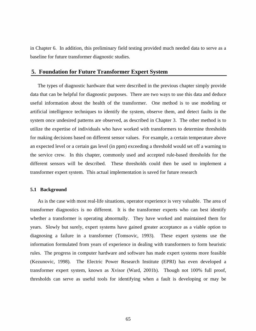
in Chapter 6. In addition, this preliminary field testing provided much needed data to serve as a

baseline for future transformer diagnostic studies.

5. Foundation for Future Transformer Expert System The types of diagnostic hardware that were described in the previous chapter simply provide

data that can be helpful for diagnostic purposes. There are two ways to use this data and deduce

useful information about the health of the transformer. One method is to use modeling or

artificial intelligence techniques to identify the system, observe them, and detect faults in the

system once undesired patterns are observed, as described in Chapter 3. The other method is to

utilize the expertise of individuals who have worked with transformers to determine thresholds

for making decisions based on different sensor values. For example, a certain temperature above

an expected level or a certain gas level (in ppm) exceeding a threshold would set off a warning to

the service crew. In this chapter, commonly used and accepted rule-based thresholds for the

different sensors will be described. These thresholds could then be used to implement a

transformer expert system. This actual implementation is saved for future research

5.1 Background As is the case with most real-life situations, operator experience is very valuable. The area of

transformer diagnostics is no different. It is the transformer experts who can best identify

whether a transformer is operating abnormally. They have worked and maintained them for

years. Slowly but surely, expert systems have gained greater acceptance as a viable option to

diagnosing a failure in a transformer (Tomsovic, 1993). These expert systems use the

information formulated from years of experience in dealing with transformers to form heuristic

rules. The progress in computer hardware and software has made expert systems more feasible

(Kezunovic, 1998). The Electric Power Research Institute (EPRI) has even developed a

transformer expert system, known as Xvisor (Ward, 2001b). Though not 100% full proof,

thresholds can serve as useful tools for identifying when a fault is developing or may be

65

imminent. Thresholds have been formed for almost all types of sensors used in transformer

diagnostics. The most commonly accepted thresholds are given below.

5.2 Dissolved Gas Analysis Thresholds As was noted in Section 2.1.1, there are several different key gases that can be used as

indicators for the development of potential failures starting in a transformer. These gases

include, but are not limited to, hydrogen, methane, ethane, acetylene, ethylene, ethane, carbon

dioxide, and carbon monoxide. Through much experience in the field, various gases have been

determined to indicate the different operating conditions. These conditions range from normal

operating conditions to severe ones. Table 5.1 (Traub, 2001) shows the limits for the key gas

concentrations in parts per million (ppm). The table is divided into four alarm levels. Normal

indicates acceptable concentration for normal operating conditions. Moderate indicates higher

than normal concentrations and suggests that some analysis should be done. High indicates a

high level of decomposition and that numerous tests should be run on the oil to establish a trend

of gas generation. From this trend, gas ratio analysis (mentioned in Section 2.1.1) can be applied

for diagnosis. Finally, severe indicates the transformer has excessive decomposition and further

operation could result in the failure of the transformer.

As described in Section 2.1.1, often the ratio of gases and the trend in gas generation is more

important than the absolute concentrations of any given gas. For example, limits have been

formed on the hydrogen content in the oil. These limits are used to indicate insulation

deterioration. Unlike the absolute limits given in Table 5.1, these limits also take into account

the rate of generation of a specific gas ratio. For hydrogen, a warning is given when there is an

increasing trend after 200 ppm of hydrogen is present and while the hydrogen to methane ratio is

5:1 or greater. This high ratio indicates partial discharge and substantiates the hydrogen contents

indication of insulation deterioration. One can see 200 ppm of hydrogen is only a moderate

condition in Table 5.1; however, when in coordination with the high ratio, it causes a concern.

66

Table 5.1: Concentration (ppm) for dissolved key gases

Danger Level

Hydroge

n

Methan

e

Acetylen

e

Ethylen

e

Ethan

e

Carbon Monoxid

e

Carbo

n Dioxide

Normal 100 120 35 50 65 350 2500 Moderat

e 101 to 700

121 to 400

36 to 50 51 to 100

66 to 100

351 to 570

2500 to 4000

High 701 to 1800

401 to 1000

51 to 80 101 to 200

101 to 150

571 to 1400

4001 to 10000

Severe >1800 >1000 >80 >200 >150 >1400 >10000

5.3 Moisture Analysis Limits Just as the dissolved gas in the oil can indicate insulation deterioration, the moisture in the oil

can prove to be just as helpful. A common limit on the moisture content in the oil has been

15ppm. The amount of oil is also dependant of the primary voltage rating of the transformer and

the temperature. For this reason, different limits have been placed based on the voltage. For less

than 345kV at 75°C, 20ppm is the limit on the moisture in the oil. On the other hand, for 345 kV

or higher at 75°C, the limit is only 10ppm. This limit criterion for moisture content is almost

universally used to indicate insulation deterioration, oil leaks, and overheating of the

transformer.

5.4 Top Oil Temperature Thresholds Thresholds and limits are most commonly used with temperature measurements, especially

of the top oil. Main tank, top oil, bottom oil, and hot spot temperatures are all common

temperature measurements that are taken. Overheating is a sure sign of insulation and oil

deterioration. Experts commonly use a green, yellow, red system to indicate the condition of the

transformer. Green indicates normal operating conditions. Yellow indicates reason for further

analysis to be performed. Red indicates impending failure if the transformer remains in

67

operation. Table 5.2 shows the limit criteria for the top oil temperature and the related

categorization.

Table 5.2: Warning categories for top oil temperature

Warning Level Temperature Range

Green T<90°C Yellow 90°C<T<100°C

Red T>100°C

Many times instead of an absolute value for a temperature limit, temperatures above a

reference are used to determine when a transformer is in danger of failing. The normal

temperature reference is determined by the age and type of transformer being monitored. In this

case, the warning categories used differ from the levels given in Table 5.2. The temperature

categories for oil temperature above a reference is given in Table 5.3.

Table 5.3: Warning categories for top oil temperature above reference

Warning Category Temperature above Reference

Minor T<10°C Intermediate 10°C<T<29°C

Serious 30°C<T<50°C Critical T>50°C

68

5.5 Vibration Levels Though not as commonly used, various warning levels have also been developed for

vibration readings. While the frequency spectra of the vibration often proves more valuable,

excessive vibrations on the shell of a transformer can often be an indication of some malfunction

of the transformer. The pumps or fans may no longer be operating properly. The coils or

magnetic core may have been jarred loose. All of these malfunctions may ultimately lead to a

transformer failure. For this reason, the magnitude of the vibration on the shell of the

transformer can be an indicator of a failing transformer or one that needs to be examined or

serviced. Table 5.4 provides the warning levels that have been formed for vibration

measurements in order to warn of problems with the transformer.

Table 5.4: Warning categories for shell vibration readings

Warning Category Vibration Reading (in/s)

Minor 0.10<V<0.25 Intermediate 0.25<V<0.50

Serious 0.50<V<1.00 Critical V>1.00

5.6 Bushing Thermal Thresholds As noted in Section 2.1.7, the temperature of transformer bushings increases dramatically

before they fail. Unlike the case with LTCs, bushing temperatures are often compared with the

other bushings’ temperatures rather than the main tank temperature. In the case of bushings,

there are essentially two operating conditions. One, the bushing are operating normally. Two,

bushings need to be investigated for leaks, loss of seal or bad connections. The common criteria

used is the temperature differential between bushings. If one bushing’s temperature is greater

than the other two by 5°C or more, the bushing should be investigated.

69

Many bushing sensors also measure oil level in addition to temperature. In this case, an oil

level below a minimum threshold indicates that the bushing should be investigated. The

manufacturer determines the minimum oil level for proper operation.

5.7 LTC Thermal Thresholds Similar to bushing monitoring, the temperature differential between the load tap changer

(LTC) and the main tank temperature is a reliable indicator of an impending failure in the LTC

as well. As with the main tank, thresholds can be placed on the degree of temperature

differential in order to get an idea of the severity of the problem.

In the case of LTCs, the procedure and thresholds used varies with the type of load tap

changers. Through much experience in the field with Westinghouse and Federal Pacific UTT-A

and UTT-B LTCs, it has been found that if the temperature differential between the main tank

and the LTC is less than 15°C, the LTC is operating normally. When the temperature differential

rises above 15°C, measures should be taken to investigate the health of the LTC, using

knowledge of the highest and lowest tap settings in the past 60 days. It is important to consider

the abruptness of the rise in the temperature differential. If the LTC has not passed through

neutral since last reset, the contacts should be wiped and DGA monitoring should be performed.

If this is not the case and the slope to the temperature differential over the past few days is

greater than zero, a severe condition exists and the LTC should be taken offline and inspected

internally to determine the problem. For Waukesha type LTCs, the procedure and tests are the

same except for the temperature differential indicating a possible problem is 5°C instead of

15°C. Series of other if/then statements have been formed for other types of LTCs as well but

shall not be discussed here.

The above thresholds and levels for different transformer diagnostic sensors have been

developed based on the knowledge and best judgment of experts in the field. These limits are by

no means a guarantee. A transformer may fail when all indicators point to normal. Likewise, a

transformer may be able to operate properly for years after a warning has been given. In

70

addition, expert systems have the drawback that they require a wide knowledge base for

diagnosis. Often, this knowledge base is not sufficient to translate the appropriate rules. The

expert system knowledge base can never be perfect (Xu, 1997). For this reason, people have

sought alternate ways to diagnose a transform using sensor data.

5.8 Fusion into Expert System The various thresholds described above do not qualify as an expert system in themselves. In

creating the expert system, a series of IF/THEN statements must serve to connect the various

sensor measurements. For example, it is known that a rise in the acetylene concentration with

respect to the ethylene concentration indicates arcing occurring in the transformer. Arcing will

also cause a rise in the top oil temperature. To validate the arcing hypothesis, the temperature

over reference measurement should also be checked. There is always the possibility of sensor

failure, which could set off a warning but not be indicative of a developing failure.

The goal of monitoring substation equipment is to prevent catastrophic failures, but also

eliminate unnecessary maintenance. By creating an expert system, the idea is to prevent

incorrect diagnosis by coordinating the thresholds from several different, but related,

measurements. Through this coordination, incorrect warnings based on one threshold can be

validated using other measurements as well. Below is an example of coordinated statements

incorporated into an expert system in order to detect transformer overheating.

IF (Temperature Above Reference) > 20°C THEN IF (Fan Bank Current) > 0.5 A THEN IF (Ethylene Concentration) > 100 ppm THEN IF (Moisture Concentration) > 15 ppm THEN Transformer Overheating, Take 0ff-line to Service ELSE Check DGA and Moisture Analyzer for Proper Functioning ELSE

71

Check Thermocouple Sensor ELSE Fan Bank not Operating Properly, Have Serviced ELSE Transformers Operating Normally

From the example, it can be observed how several sensor measurements and their respective

thresholds are utilized to make a diagnosis. First, the temperature sensor is checked to see if

there is any overheating. If there is an abnormal reading, the current to the fan banks are

checked. If the fans are running, the ethylene, which indicates high temperature oil deterioration,

is checked to make sure the level is high. If the ethylene level is above normal, the moisture in

the oil is checked. If at any point, a sensor does not confirm the diagnosis of a previous sensor;

the proper functioning of the sensor is checked. In this piecewise method, it is possible to

deduce if a failure is occurring or if sensors are simply malfunctioning.

In many cases, all the sensor measurements may not be available. It is not necessary to have

numerous sensors indicating the same information. The chances of two different sensors failing

at the same time and producing an incorrect warning signal is highly improbable. It should be

noted that the sensor order to be used is dependent on the type of failure being detected. To

detect an arcing failure, the ratio of acetylene to ethylene should probably be the predominant

measurement.

Every expert system that is created will consist of numerous set of IF/THEN possibilities like

the one given above. The design of each expert system will be different depending on the sensor

measurements available and the type of failures being detected. The key to a successful expert

system is to utilize all knowledge known about the system and to provide for checks in the

system, so that no one measurement is used to diagnose the health of the equipment.

5.9 Proposed Hybrid Diagnostic System In the previous section, the method for creating an expert system from common sensor

thresholds was discussed. There are many problems with simply using an expert system to

72

diagnose the health of a transformer. There are still many types of failures for which thresholds

have not been established. There are also many failures that are only indicated by a particular

sensor measurement. Therefore, there is no way to validate the expert system diagnosis with

another sensor measurement. In Chapter 3, an artificial intelligent technique for transformer

diagnostics was described. This neuro-fuzzy fault detector creates its own rule-base using

simply input-output data. However, the system would need a database detailing all types of

faults to provide full-proof diagnosis. There is always need for additional information to

incorporate into its “neurons.”

The shortcomings to both the expert system and the neuro-fuzzy network can be overcome

by creating a diagnostic system that combines the two techniques. The neuro-fuzzy network can

set alarms when the system begins to behave abnormally. At the same time, the expert system

thresholds can be applied to determine what may be the failure responsible for this abnormality.

Likewise, a warning detected by the expert can be used to indicate when the neural network may

be lacking experience. In this way, the expert system can highlight events where the neuro-fuzzy

network needs to be trained. Much like the expert system, this hybrid diagnostic system would

use the two techniques to combine the best of human and artificial intelligence. A block diagram

of this approach is shown in Figure 5.1.

The full potential of this hybrid diagnostic system will not be achieved until the neuro-fuzzy

network has witnessed many different failures and a more complete human knowledge base is

formed for the various failure modes. Due to the lack of dissolved gas or moisture analyzers in

the diagnostic module designed in this thesis, only the foundation for a hybrid diagnostic system

is given here. The experimental results for the neuro-fuzzy fault detector are presented in the

next chapter.

73

Figure 5.1: Block diagram of hybrid diagnostic approach

6. Experimental Analysis As mentioned in Chapter 4, the monitoring system designed and developed in this research is

being tested on three single-phase 166 MVA transformers at WAPA’s Ault substation located in

northern Colorado. This chapter focuses on the result of applying the neuro-fuzzy fault detection

engine to analyze the data that is obtained by the diagnostic monitoring system of Chapter 4. A

detailed look into the results of the system identification, output estimation, and fault detection

for the three transformers is given in this chapter.

6.1 Off-line Fault Detection Analysis As described in Chapter 4, the diagnostic module designed for monitoring transformers is

able to collect, manipulate, and send temperature, current, and vibration data to the substation

computer. Then a dial-up modem can be used to acquire the data for off-line data analysis by the

neuro-fuzzy fault detection engine. For the purposes of experimental analysis, this off-line

74

method is used as opposed to the on-line method. It is also possible to use the monitoring system

in coordination with the fault detector for on-line analysis. In this case, the MATLAB or C

coding for the system can be installed on the substation computer to analyze the data as it is

collected and transmitted by the diagnostic module.

The neural network must be trained to the system before the on-line fault detection can be

performed. For the experimental analysis done in this research, the data from the diagnostic

module was collected for several weeks before it was transferred to the computer at Colorado

School of Mines. The neuro-fuzzy engine implemented in MATLAB could then analyze the

data. In the preliminary stages, different sensors were used as the inputs and outputs to

determine which configuration yielded the best system identification and observation. Off-line

monitoring was utilized for this reason.

6.2 Non-linear System Identification

Once the data had been collected and transferred to the computer at Mines for analysis by the

neural network, the problem then became determining which sensor measurements should be

used as inputs and outputs for system identification. The robustness of the system identification

can vary greatly depending on the number and type of measurements used. The ability of the

neural network to locate the global minimum is very sensitive. For this reason, many different

combinations of sensor inputs and outputs were tried. The different combinations had a

relatively large effect on the mean squared error of the training. The natural choice was to make

the transformer currents (primary, secondary, and tertiary) as well as the pump and fan bank

currents inputs to the system. In addition to these current measurements, the ambient

temperature and top tank temperature were used as inputs. The ambient temperature provided

information to the external conditions, while the top tank temperature provided a measure of

transformer operation. The main tank temperature was the temperature output. Due to the

importance of the lower odd harmonics in determining coil loosening as mentioned in Chapter 2,

these frequencies were also used as inputs and outputs. The seventh and ninth harmonics were

75

used as inputs, while the third and fifth harmonics were the outputs. This combination provided

the best results for the training sets.

Table 6.1 gives a list of the sensor measurements used for system identification given the

transformer data provided by the diagnostic module. The model structure for the chosen set of

input and output measurements is given in Equation (6.1).

Table 6.1: Input output measurements used for transformer models

Sensor Measurement Point Type T1 Main Tank Temperature Output 1 V1 Vibration of Third Harmonic Output 2 V2 Vibration of Fifth Harmonic Output 3 T2 Top Tank Temperature Input 1 TA Ambient Temperature Input 2 C1 Primary Current Input 3 C2 Secondary Current Input 4 C3 Tertiary Current Input 5

CP1 Fan and Pump Bank Current #1 Input 6 CP2 Fan and Pump Bank Current #2 Input 7 V3 Vibration of Seventh Harmonic Input 8 V4 Vibration of Ninth Harmonic Input 9

))(),(),(),(),(),(),(),(),(),(),(),(()1()1()1(

43213212211

2

1

1

kukukukukukukukukukykykyFkykyky

VVCPCPCCCTATVVT

V

V

T

=⎥⎥⎥

⎦

⎤

⎢⎢⎢

⎣

⎡

+++

(6.1)

For all three transformers, data collected over the same nine-day period was used to train the

neural network. Though shorter periods of time can be used for training, it was found that a

nine-day period provided a more accurate identification of the system that was more robust. As

mentioned in Chapter 3, varying numbers of membership functions can be used during the

training and simulation of the TNFIN neural network. A greater number of membership

functions will provide a higher accuracy; however, the training time and the memory

requirements increase significantly as the number of membership functions increases. One can

76

think of the membership functions as linguistic values, such as low, medium, high. If there are

six membership functions, this means there are 6 fuzzy sets for each input. The neural network

determines the degree that each input belongs in each set. The amount of membership functions

to use is best determined through trial trainings. For the training of all three transformers used in

this experiment, four membership functions per input were used. Through experimentation with

up to 12 membership functions per input, the improvement in accuracy was not significant

enough to justify the use of more than four membership functions, especially given the added

memory that is required. The shape of the four membership functions for the top tank

temperature (input 1) for the training of Transformer A is given in Figure 6.1. The membership

functions are bell-shaped and slightly overlap, as is to be expected. Figures 6.1-6.12 show the

inputs and outputs that were used for the training of Transformer A.

0.57 0.58 0.59 0.6 0.61 0.62 0.63 0.640

0.2

0.4

0.6

0.8

1

Membership Functions for Top Tank Temperature Input of Transformer A

Normailized Input

Mem

bers

hip

Deg

ree

Figure 6.1: Four membership functions of Transformer A’s top tank temperature input

77

0 2000 4000 6000 8000 10000

0.58

0.59

0.6

0.61

0.62

Transformer A System Input (Top Tank Temperature)

Time (min.)

Nor

mal

ized

Dat

a

Figure 6.2: Transformer A system input-top tank temperature

0 2000 4000 6000 8000 100000.54

0.55

0.56

0.57

0.58

0.59

0.6

0.61

0.62Transformer A System Input (Ambient Temperature)

Time (min.)

Nor

mal

ized

Dat

a

Figure 6.3: Transformer A system input-ambient temperature

78

0 2000 4000 6000 8000 100000.1

0.15

0.2

0.25

0.3

0.35

0.4

0.45Transformer A System Input (Primary Current)

Time (min.)

Nor

mal

ized

Dat

a

Figure 6.4: Transformer A System Input-Primary Current

0 2000 4000 6000 8000 100000.1

0.2

0.3

0.4

0.5

0.6

0.7

0.8Transformer A System Input (Secondary Current)

Time (min.)

Nor

mal

ized

Dat

a

Figure 6.5: Transformer A system input-secondary current

79

0 2000 4000 6000 8000 100000

0.1

0.2

0.3

0.4

0.5

Transformer A System Input (Tertiary Current)

Time (min.)

Nor

mal

ized

Dat

a

Figure 6.6: Transformer A system input-tertiary current

0 2000 4000 6000 8000 100000.8

0.82

0.84

0.86

0.88

0.9

0.92

0.94

0.96

0.98

1

Time (min.)

Nor

mal

ized

Dat

a

Transformer A System Input (Fan and Pump Bank Current #1)

Figure 6.7: Transformer A system input-fan and pump bank current #1

80

0 2000 4000 6000 8000 10000

0.64

0.66

0.68

0.7

0.72

0.74

0.76

0.78

0.8

Transformer A System Input (Fan and Pump Bank Current #2)

Time (min.)

Nor

mal

ized

Dat

a

Figure 6.8: Transformer A system input-fan and pump bank current #2

0 2000 4000 6000 8000 100000.1

0.2

0.3

0.4

0.5

0.6

0.7

0.8Transformer A System Input (7th Harmonic Vibration)

Time (min.)

Nor

mal

ized

Dat

a

Figure 6.9: Transformer A system input-7th harmonic vibration

81

0 2000 4000 6000 8000 100000

0.1

0.2

0.3

0.4

0.5

0.6

Transformer A System Input (9th Harmonic Vibration)

Time (min.)

Nor

mal

ized

Dat

a

Figure 6.10: Transformer A system input-9th harmonic vibration

0 2000 4000 6000 8000 10000

0.575

0.58

0.585

0.59

0.595

0.6

0.605

0.61

0.615

0.62

Transformer A System Output (Main Tank Temperature)

Time (min.)

Nor

mal

ized

Dat

a

Figure 6.11: Transformer A system output-main tank temperature

82

0 2000 4000 6000 8000 100000

0.1

0.2

0.3

0.4

0.5

0.6

0.7Transformer A System Output (3rd Harmonic Vibration)

Time (min.)

Nor

mal

ized

Dat

a

Figure 6.12: Transformer A system output-3rd harmonic vibration

0 2000 4000 6000 8000 100000.3

0.4

0.5

0.6

0.7

0.8

0.9

1Transformer A System Output (5th Harmonic Vibration)

Time (min.)

Nor

mal

ized

Dat

a

Figure 6.13: Transformer A system output-5th harmonic vibration

83

From the above graphs, one notices that the inputs and outputs have all been normalized.

This was done by finding the maximum value of any given input or output and dividing that

input or output by a number about 50% larger than the maximum. This assures that the inputs

and outputs will never have a value greater than 1. This is necessary because the TNFIN only

accepts inputs and outputs between 0 and 1. The same normalization factor was used for training

and simulation so that the parameters (a,b,c,d) determined during training would be appropriate

for simulation as well.

The results of the TNFIN training are shown in Figure 6.14-6.22. The network did a fairly

good job of training. The mean squared error was around .001 for all three phases. Given the

noise present in the system and variation in the measurements, this error is more than acceptable

for training purposes. The network struggled with identification for the vibration outputs but

provided accurate temperature identification. Table 6.2 gives a summary of the training results

for the three transformers.

Table 6.2: Summary of training results for three transformers (A-C)

Transformer A Transformer B Transformer C

Number of Inputs 9 9 9 Number of Outputs 3 3 3

Number TNFIN Nodes 183 183 183 Sample Size 11256 10753 11256

Mean Squared Error (MSE) .0022 .0012 .00091 Training Time 99.593 95.036 96.028

84

0 2000 4000 6000 8000 10000

0.58

0.59

0.6

0.61

0.62

0.63

Transformer A TNFIN Training versus Actual (Main Tank Temperature)

Time (min.)

Nor

mal

ized

Dat

aActualEstimate

Figure 6.14: Transformer A TNFIN training versus actual-main tank temperature

0 2000 4000 6000 8000 100000

0.1

0.2

0.3

0.4

0.5

0.6

Transformer A TNFIN Training versus Actual (3rd Harmonic Vibration)

Time (min.)

Nor

mal

ized

Dat

a

ActualEstimate

Figure 6.15: Transformer A TNFIN training versus actual-3rd harmonic vibration

85

0 2000 4000 6000 8000 100000.3

0.4

0.5

0.6

0.7

0.8

0.9

1Transformer A TNFIN Training versus Actual (5th Harmonic Vibration)

Time (min.)

Nor

mal

ized

Dat

aActualEstimate

Figure 6.16: Transformer A TNFIN training versus actual-5th harmonic vibration

0 2000 4000 6000 8000 100000.57

0.58

0.59

0.6

0.61

0.62

0.63Transformer B TNFIN Training versus Actual (Main Tank Temperature)

Time (min.)

Nor

mal

ized

Dat

a

ActualEstimate

Figure 6.17: Transformer B TNFIN training versus actual-main tank temperature

86

0 2000 4000 6000 8000 100000

0.05

0.1

0.15

0.2

0.25

0.3

0.35

0.4

0.45Transformer B TNFIN Training versus Actual (3rd Harmonic Vibration)

Time (min.)

Nor

mal

ized

Dat

aActualEstimate

Figure 6.18: Transformer B TNFIN training versus actual-3rd harmonic vibration

0 2000 4000 6000 8000 100000.1

0.2

0.3

0.4

0.5

0.6

0.7

0.8

0.9Transformer B TNFIN Training versus Actual (5th Harmonic Vibration)

Time (min.)

Nor

mal

ized

Dat

a

ActualEstimate

Figure 6.19: Transformer B TNFIN training versus actual-5th harmonic vibration

87

0 2000 4000 6000 8000 100000.585

0.59

0.595

0.6

0.605

0.61

0.615

0.62

0.625

0.63

Transformer C TNFIN Training versus Actual (Main Tank Temperature)

Time (min.)

Nor

mal

ized

Dat

aActualEstimate

Figure 6.20: Transformer C TNFIN training versus actual-main tank temperature

0 2000 4000 6000 8000 100000.2

0.3

0.4

0.5

0.6

0.7

0.8

0.9

1

Transformer C TNFIN Training versus Actual (3rd Harmonic Vibration)

Time (min.)

Nor

mal

ized

Dat

a

ActualEstimate

Figure 6.21: Transformer C TNFIN training versus actual-3rd harmonic vibration

88

0 2000 4000 6000 8000 100000

0.1

0.2

0.3

0.4

0.5

0.6

0.7Transformer C TNFIN Training versus Actual (5th Harmonic Vibration)

Time (min.)

Nor

mal

ized

Dat

aActualEstimate

Figure 6.22: Transformer C TNFIN training versus actual-5th harmonic vibration

6.3 Model Validation and Output Estimation Once the neural network has formed a model based on a training set, the robustness of this

model must be validated using sample data not contained within the training set. Often times,

the neural network may struggle to give accurate estimates of the system outputs during sample

simulations. Therefore, another 9-day data set was used to validate the neural network training.

The neural network was found to be fairly robust for the temperature estimates with the error

lying below 0.01 (equivalent to several degrees Celsius). The network struggled more with the

vibration estimates. Here, the error between actual and estimate are as high as 0.3 at times. This

is less alarming given the normalization factor for the vibration was twenty times less than for

the temperature. A plot of the error in validation for the three outputs is given in Figures 6.23-

6.25.

89

0 1000 2000 3000 4000 5000 6000 7000

-0.01

0

0.01E

rror

Tranformer A Validation Data

Main Tank Temperature

0 1000 2000 3000 4000 5000 6000 7000-0.5

0

0.5

Err

or

3rd Harmonic Vibration

0 1000 2000 3000 4000 5000 6000 7000-0.5

0

0.5

Err

or

Time (min.)

5th Harmonic Vibration

Figure 6.23: Transformer A neural network validation

0 1000 2000 3000 4000 5000 6000 7000

-0.01

0

0.01

Err

or

Tranformer B Validation Data

Main Tank Temperature

0 1000 2000 3000 4000 5000 6000 7000-0.5

0

0.5

Err

or

3rd Harmonic Vibration

0 1000 2000 3000 4000 5000 6000 7000-0.5

0

0.5

Err

or

Time (min.)

5th Harmonic Vibration

Figure 6.24: Transformer B neural network validation

90

0 1000 2000 3000 4000 5000 6000 7000-0.01

0

0.01E

rror

Tranformer C Validation Data

Main Tank Temperature

0 1000 2000 3000 4000 5000 6000 7000-0.5

0

0.5

Err

or

3rd Harmonic Vibration

0 1000 2000 3000 4000 5000 6000 7000-0.5

0

0.5

Err

or

Time (min.)

5th Harmonic Vibration

Figure 6.25: Transformer C neural network validation

One must also be aware that the starting point of the neural network can greatly affect the

robustness and observability of the outputs. The neural network will often struggle for a period

of time before it recognizes a point with which it is familiar. For this reason, it is recommended

to overlap the beginning of the sample set with a portion of the training set. However, even

when doing this, it will sometimes take the network a period of time before it produces accurate

estimates. An example of the recognition time of the neural network is given in Figure 6.26. It

took the trained neural network of Transformer A until the 6000th minute before it produced

accurate estimates. One should note that this can occur during short periods of time, and that the

fault detection engine should not send out a warning unless the error stays above a threshold for

a sustained time.

91

0 2000 4000 6000 8000 10000 12000

0.57

0.58

0.59

0.6

0.61

0.62

0.63

Time (min.)

Nor

mal

ized

Out

put

Recognition Time For Transformer A

ActualEstimate

Figure 6.26: Recognition time for neural network training of transformer A

6.4 Fault Detection As illustrated in Chapter 3, non-linear system identification and output estimation are the two

preliminary steps toward fault detection. Now that the non-linear system dynamics have been

identified and proven to give robust estimates of the outputs (in particular the temperature), the

desired goal of fault detection can be achieved. There are two different types of failures that can

occur and be detected by the neuro-fuzzy system. These are actual system failures and hardware

(i.e. sensor) failures. The successful detection of these two types of failures is discussed in the

next two sections.

6.4.1 System Failure As might be expected, witnessing an actual fault to occur over a six month period for a

transformer, whose average life is around 40 years, is not highly probable. During this research,

the statistics held true and no transformer fault was witnessed on any of the three transformers

92

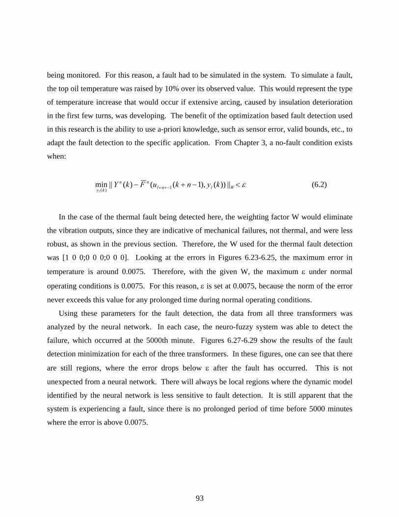
being monitored. For this reason, a fault had to be simulated in the system. To simulate a fault,

the top oil temperature was raised by 10% over its observed value. This would represent the type

of temperature increase that would occur if extensive arcing, caused by insulation deterioration

in the first few turns, was developing. The benefit of the optimization based fault detection used

in this research is the ability to use a-priori knowledge, such as sensor error, valid bounds, etc., to

adapt the fault detection to the specific application. From Chapter 3, a no-fault condition exists

when:

ε<−+− −++ Wlnlnn

kykynkuFkY

l

||))(),1(()(||min 1)( (6.2)

In the case of the thermal fault being detected here, the weighting factor W would eliminate

the vibration outputs, since they are indicative of mechanical failures, not thermal, and were less

robust, as shown in the previous section. Therefore, the W used for the thermal fault detection

was [1 0 0;0 0 0;0 0 0]. Looking at the errors in Figures 6.23-6.25, the maximum error in

temperature is around 0.0075. Therefore, with the given W, the maximum ε under normal

operating conditions is 0.0075. For this reason, ε is set at 0.0075, because the norm of the error

never exceeds this value for any prolonged time during normal operating conditions.

Using these parameters for the fault detection, the data from all three transformers was

analyzed by the neural network. In each case, the neuro-fuzzy system was able to detect the

failure, which occurred at the 5000th minute. Figures 6.27-6.29 show the results of the fault

detection minimization for each of the three transformers. In these figures, one can see that there

are still regions, where the error drops below ε after the fault has occurred. This is not

unexpected from a neural network. There will always be local regions where the dynamic model

identified by the neural network is less sensitive to fault detection. It is still apparent that the

system is experiencing a fault, since there is no prolonged period of time before 5000 minutes

where the error is above 0.0075.

93

Figure 6.27: Result of fault detection for transformer A

Figure 6.28: Result of fault detection for transformer B

94

Figure 6.29: Result of fault detection for transformer C

The weighting, W, that is placed on the various outputs when determining the error

minimization will be dependant on the fault being detected. A mechanical fault would place

more emphasis on the vibration outputs instead of the temperature output, as illustrated in this

example.

6.4.2 Sensor Failure

In the previous section, it was seen how a change in the dynamics can be detected using the

TNFIN network. This change can be caused by a developing failure in the system, as simulated

in the last section, or by a faulty sensor. In order to prevent errant diagnosis of a transformer’s

health, additional processing is required. A faulty sensor can be detected and isolated by using

only some of the outputs when performing the optimized fault detection. In other words, it is

assumed that there is no knowledge about one of the outputs. By removing one output sensor at

a time, it can be determined if the detected change is caused by a sensor or is actually indicative

of a developing fault in the system.

95

The method for detecting a sensor failure is best illustrated by an example. The sample data

from Transformer C is used. All three outputs are used in the error minimization; however, the

temperature measurement is weighted ten times more to compensate for the difference in

normalization factor. At time (t = 5000), the first vibration sensor fails and begins to produce

inaccurate outputs. This failure is induced by eliminating the lowest frequency output of the

accelerometer, thus simulating an accelerometer that can no longer detect low frequencies.

When all sensors are considered, it is seen that a fault has occurred, since the error exceeds ε.

The top-left graph of Figure 6.30 illustrates this fact. One by one a sensor is ignored. A fault is

still detected in every case, as shown in Figure 6.30, except when sensor V1 is removed.

Therefore, V1 must be a faulty sensor. A more detailed and processing intensive procedure can

be utilized to determine an input sensor fault. In this case, the neural network must be retrained

to identify the system with one less input and then the same procedure is followed, removing one

input sensor at a time. This method may not work for inputs that are critical to accurate system

identification.

6.4.3 System and Sensor Failure There is always the possibility that a sensor may fail at the same time that the system is

experiencing a failure. Sometimes a system failure may cause a sensor failure. It is desired that

the fault detector be able to detect and isolate both failures. If the failures occur at a different

times with the sensor occurring first, it is easy to see how the TNFIN fault detector could detect

both faults. By using the approach of the previous section, one could see there would be a

shorter period of failure when the faulty sensor was removed, thus indicating that both a sensor

and system failure had occurred but at different times. The problem becomes detecting both

failures when they occur simultaneously. As an example, the system and sensor faults that were

simulated in the past two sections now occur at nearly the same time. Since a thermal fault is

being detected, more weight is placed on the temperature output just as in the previous section.

96

0 2000 4000 6000 80000

0.01

0.02

0.03

0.04

0.05

Err

orNo Sensor Removed

0 2000 4000 6000 80000

0.01

0.02

0.03

0.04

0.05

Err

or

T1 Sensor Removed

0 2000 4000 6000 80000

0.01

0.02

0.03

0.04

0.05

Time (min.)

Err

or

V1 Sensor Removed

0 2000 4000 6000 80000

0.01

0.02

0.03

0.04

0.05

Time (min.)

Err

or

V2 Sensor Removed

Figure 6.30: V1 sensor failure, detection and isolation of sensor failure

Figure 6.31 shows the results of removing the sensors one at a time and seeing if the faults

are still detected. Here, a problem is detected. There are obviously some spikes that are created

by the sensor failure at around 6000 minutes. In all three graphs, there is a short period of time

where a fault is detected and ε is exceeded, namely at around 5000 minutes. However, much of

the information about the system failure has been lost. It is difficult to distinguish if a system

failure has occurred or simply a sensor failure. This is one area where the TNFIN fault detector

lacks. It is difficult to distinguish between residuals caused by system failures and those caused

by sensor failures, if they occur at the same time.

97

0 2000 4000 6000 80000

0.01

0.02

0.03

0.04

0.05E

rror

No Sensor Removed

0 2000 4000 6000 80000

0.01

0.02

0.03

0.04

0.05

Err

or

T1 Sensor Removed

0 2000 4000 6000 80000

0.01

0.02

0.03

0.04

0.05

Time (min.)

Err

or

V1 Sensor Removed

0 2000 4000 6000 80000

0.01

0.02

0.03

0.04

0.05

Time (min.)

Err

or

V2 Sensor Removed

Figure 6.31: Detection and isolation and system and sensor failure

In summary, using the neuro-fuzzy system described in Chapter 3, the non-linear transformer

dynamics were identified. Robust output estimates could then be made, which allowed for

optimized fault detection. The fault detection method could distinguish between system and

sensor failures. The fault detection capability can be improved by training with larger data sets,

in order to capture more of the system dynamics and thus form a better model. Actual

transformer faults must be witnessed before full validation of the fault detection engine can be

verified.

98

7. Conclusions and Future Work 7.1 Summary Much important advancement was reached from the research described in this report. A

transformer diagnostic system that could be implemented on large scale, field-level equipment

was developed and tested. The neuro-fuzzy fault detection engine developed and validated on a

small 10kVA distribution transformer was implemented on three large substation transformers.

Through this field implementation, valuable information was gained about the diagnostic module

needed for monitoring and how the neuro-fuzzy system can be utilized to provide the maximum

fault detecting capability. The major contributions of this research are summarized in the

following sections.

7.1.1 Diagnostic Hardware Module

• A diagnostic module was designed and three prototypes were manufactured. This

diagnostic module included the non-invasive sensors that have been found to indicate

developing faults in transformers. The system also included its own power supply, signal

conditioner, DAQ card, and PC104 to process the data from the sensors. The module was

also equipped with a RS232 to fiber converter to send the data in the noisy substation

environment

• The diagnostic module is magnetically mounted to the inside of the transformer cabinet,

making the system easily installable and portable. The diagnostic module could be

completely installed on a transformer in less than an hour once the AC power connection

has been established.

• The three diagnostic module prototypes were placed on three single-phase transformers at

the Ault substation. They were placed in the harsh environment starting in the summer

99

months and continuing into the winter. The modules successfully collected data during

these varying weather conditions proving their durability.

7.1.2 Data Manipulation and Communication • The appropriate software was written in C for both the PC104 located on the diagnostic

module and the computer located inside the substation house. The PC104 converted the

temperature and current data to their appropriate values and performed an FFT on the

accelerometer data.

• Data was sent from the PC104 to the substation computer at one-minute intervals. The

substation computer saved the data as strings in date marked files. A GUI was placed on

the substation computer to allow maintenance personnel to see the sensor outputs and the

FFTs.

• Substation computer connected through modem to CSM computer. The modem did not

sacrifice substation security, but allowed for easy access to data. The installation of

RealVNC allowed for remote control over the system through the substation desktop.

7.1.3 Non-linear System Identification and Fault Detection • System identification and fault detection was applied to three large 166 MVA

transformers at the Ault substation using the data obtained from the diagnostic module

designed in this research. Using current, ambient and top tank temperatures, and certain

frequencies as inputs, the main tank temperature as well as certain vibration frequencies

were predicted using the TNFIN. The experiments showed that the temperature

dynamics could be accurately identified using the TNFIN. The TNFIN struggled more

with the vibration dynamics but still provided decent estimates of the highly varying

outputs.

• After identifying the system through training, the TNFIN was used to estimate the

outputs for a validation data set. The estimates could then be compared with the actual

100

sensor measurements. The neural network was found to be relatively robust. However,

the neural networks estimates were highly sensitive to starting positions and could result

in large errors due to poor output observability.

• Fault detection was successfully achieved on the transformer by simulating a thermal

fault in the system, which would be representative of internal insulation deterioration.

• The ability of the neuro-fuzzy fault detection engine to distinguish between sensor fault

and system fault was also successfully documented through setting the outputs of one

sensor to zero, simulating a malfunctioning sensor condition. By eliminating the

knowledge of one output sensor at a time, the location of the faulty sensor was found.

7.1.4 Foundation for Hybrid Neuro-fuzzy Expert System

• The framework and preliminary rule-base for a hybrid neuro-fuzzy expert system was

presented. The system would combine the most accepted sensor threshold levels with the

neuro-fuzzy fault detection engine of this research to provide a reliable transformer health

diagnosis. The final architecture of the system will have to be adjusted as the neuro-

fuzzy system increases its knowledge base through witnessing and experiencing a variety

of failures.

7.2 Future Work The research presented in this research focused on validation and implementation of the

neuro-fuzzy fault detection engine on large substation transformers. This validation was

accomplished through the design of a diagnostic module, which could non-invasively collect

data that has been shown to provide diagnostic information about the health of transformers.

This data was then transferred to the neuro-fuzzy detection engine via a modem. From this point

in the research, there are several areas for possible future work. The major areas of study are

given below.

101

• This research focused on the implementation of the diagnostic module on three single-

phase transformers of the same age and type. However, in order for the neural network to

provide more accurate identification for many different types of transformers, a larger

database with data from many different models and years of operation is required. For

this reason, one area of possible future research is to implement the system described in

this thesis on many more transformers. Through this, it is hoped that the system will

actually witness different failures and be able to train itself to different types of behavior,

normal and abnormal.

• The work of this thesis focused on transformer diagnostics. However, the diagnostic

module and fault detection system can easily be expanded to include circuit breakers and

other substation equipment. This research could focus on using the diagnostic system

presented in this thesis for fault diagnosis of all substation equipment. This would

ultimately lead to the final goal of an intelligent substation.

• Research has focused on diagnostics at the individual substation level. Work can be done

to integrate the diagnostics and health information of several substations together into one

network. By doing so, the neuro-fizzy system could see more types of failures and train

itself to different health conditions. In addition, the network would be able to provide

information to the utility about the health of the grid and what areas may be aging and

need replacement. The network could send out warnings when one substation is having

problems so that other substations could compensate.

• The experimental results obtained in this research only used the neural network for non-

linear system identification and fault detection. Future work could utilize the output

observer by training with measurements of the dissolved gas content in the oil and then

estimating this after training is complete. It is known that DGA data provides valuable

diagnostic information; however, on-line DGA analyzers are expensive. By training with

the DGA data and then using the observer once the network is trained, it is possible to

102

achieve both accurate diagnostic capability as well as a more economically feasible

diagnostic system.

• The foundation for a hybrid neuro-fuzzy expert system was presented in this report. The

most valuable and accepted sensor thresholds were detailed. The implementation of

these thresholds into an expert system that could be combined with the neural-fuzzy fault

detection engine for more accurate fault detection is a major area for future research

endeavors.

• The diagnostic module designed in this research still required a fiber optic connection to

the substation house in order to transfer the data. This limits the portability and increases

the work needed for installation. An area of future research could focus on the

development of hardware and signal processing module that would utilize wireless

communication.

• Finally, there is also a great amount of work that can be done in the area of pattern

recognition of faults and life expectancy. Once a large database of data has been

collected from several different transformers and different types of faults have been

witnessed, it will be possible to try to classify behaviors and how they relate to

impending failures. In the long term, the pattern classification could lead to life

expectancy predictions for the transformer.

Transformer and substation diagnostics is an expanding field of study. The diagnostic

module and fault detection system presented in this thesis can be altered and expanded to provide

more and more valuable information on the health of substation equipment. The potential of this

system is vast and with further investigation, the concept of an Intelligent Substation can be

realized.

103

8. References Akcay, H., Islam, S., and Ninness, Brett. 1999. Subspace-based Identification of Power

Transformer Models from Frequency Response Data. IEEE Transactions on Instrumentation and Measurement, 48(3), pp. 700-704.

Alessandri, A. and Parisini, T. 1997. Direct Model-based Fault Diagnosis Using Neural Filters

Pages 343-348 of: Proceedings of the IFAC Conference on Fault Detection, Supervision and Safety for Technical Processes.

Archer, W.E., Deveney, M.F., and Nagel, R.L. 1994. Non-linear Transformer Modeling and

Simulation. Midwest Symposium on Circuits and Systems, 1, pp. 665-669. Baumann, W.T. and Rugh, W.J. 1986. Feedback Control of Nonlinear Systems by Extended

Linearization. IEEE Transactions on Automatic Control, AC(31), pp. 40-46. Bengtsson, T., Kols, S., and Jonsson, B. 1997. Transformer PD Diagnosis Using Acoustic

Emission Technique. Page 115 of: Proceedings of ISH-97. Montreal, Canada, 4. Berler, Z., Golubev, A., Rusov, V., Tsvetkov, V., and Patterson, C. 2000. Vibro-Acoustic

Method of Transformer Clamping Pressure Monitoring. Pages 263-266 of: Conference record of IEEE International Symposium on Electrical Insulation. Anaheim, CA.

Chen, T. and Chen, H. 1991. Universal Approximation to Nonlinear Operators by

Neural Networks with Arbitrary Activation Functions and Its Application to Dynamical Systems. IEEE Transactions on Neural Networks, 2(2), pp. 302-309.

Christian, J., Feser, K., Sundermann, U., and Leibfried, T. 1999. Diagnostics of Power

Transformers by Using the Transfer Function Method. In: Proceedings of the 11th International Symposium on High Voltage Engineering. London, United Kingdom.

Chu R., Shoureshi, R., and Tenorio, M. 1989. Neural Networks for System Identification. In:

Proceedings of the American Control Conference. American Automatic Control Council Chu, R. and Shoureshi, R. 1994. Simultaneous Parameter Identification and State Estimation

Using Neural Networks. In: Proceedings of the 10th IFAC Symposium System Identification, IFAC.

104

Cournoyer, J.S., Little, A.D., and Newton, C. 1999. A Market View of Substation On-line Monitoring. In: Proceedings of the EPRI- Substation Equipment Diagnostics Conference.

Das, S. and Olurotimi, O. 1998. Noise Recurrent Neural Networks: The Continuous-time Case.

IEEE Transactions on Neural Networks, 9(5), pp. 913-936. Das, S. and Olurotimi, O. 1998. Noise Recurrent Neural Networks: The Discrete-time case.

IEEE Transactions on Neural Networks, 9(5), pp. 937-946. Davydov, V. 1998. Evaluation of Water Content in Transformer Insulation Systems. In:

Proceedings of Substation Equipment Diagnostics Conference VI. TR-11131. Denghua, M. 2000. A New Fuzzy Information Optimization Processing Technique for

Monitoring the Transformer. Measurements and Applications of Dielectric Materials. Conference Publication #473, pp.192-195.

Deza, F., Busvelle, E., Gauthier, J.P. and Rakotopara, D. 1992. High Gain Estimation for

Nonlinear Dynamic Systems. Systems and Control Letters, 18(4), pp. 295-299. Farquharson, R. 2000. Integrated Substation Control and equipment Monitoring and

Diagnostics-An Overview. In: Proceedings of the CEPSI 2000 Conference. Manila, Philippines.

Ficola, A.,Cava, M.L., and Magnino, F. 1997. An Approach to Fault Detection for Nonlinear

Dynamic Systems Using Neural Networks. Pages 355-360 of: Proceedings of the IFAC Conference on Fault Detection, Supervision and Safety for Technical Processes.

Frank, P.M. and Ding, X. 1997. Survey of Robust Residual Generation and Evaluation Methods

in Observer-based Fault Detection Methods. Journal of Process Controls, 7(6), pp. 403-424.

Fretheim, T. 2000. Fault Detection and Non-linear Output Observer Designs Using Neural

Network Models. Ph.D. thesis, Colorado School of Mines, Engineering Department. Gao, N. and Yan, Z. 2002. New Approach on Comprehensive Diagnosis of Insulation Faults in

Power Transformer. In: Proceedings of the 2002 IEEE International Symposium on Electrical Insulation. Boston, MA.

Gauthier, J.P., Hammouri, H., and Othman, S. 1992. A Simple Observer for Nonlinear

Applications to Bioreactors. IEEE Transactions on Automatic Control, 37, pp. 875-880.

105

Griffin, P.J. 1988. Criteria for Interpretation of Data for Dissolved Gases in Oil Transformers

(A Review). Electrical Insulating Oils, STP998. American Society for Testing and Materials, Philadelphia, pp 89-106.

Hadjicostis, C.N. and Verghese, G.C. 2000. Power System Monitoring Using Petri Net

Embeddings. IEEE Proceedings C: Generation, Transmission and Distribution, 147(5), pp. 299-303.

Hagman, W.H., Kirtley Jr., J.L., Lesieutre, B.C., Boyd, M.J., Warren, E.P., Chou, H.P., and

Tabors, R.D. 1996. Model-based Monitoring of Transformers. Massachusetts Institute of Technology, Laboratory for Electromagnetic and Electronic Systems. http://power.mit.edu/transformer/paper.html, (Jan.).

Halstead, W.D. 1973. A Thermodynamic Assessment of the Formation of Gaseous

Hydrocarbons in Faulty Transformers. Journal of the Institute of Petroleum, 59, pp. 239-241.

Haykin, S. 1994. Neural Networks a Comprehensive Foundation. New York: Macmillian

College Publishing Company. Hu, Z., Shoureshi, R., Torgerson, D., and Work, J. 2000. Tsukamoto-type Neural Fuzzy

Inference Network. In: Proceedings of the American Control Conference. Huang, Y., Chang, H., and Huang, C. 1997. Developing a New Transformer Fault Diagnosis

System through Evolutionary Fuzzy Logic. IEEE Transactions on Power Delivery, 12(2), pp. 761-767.

Jota, Patricia, Islam, R.S., Syed, M., Wu, Tony, and Ledwich, G. 1998. Class of Hybrid

Intelligent System for Fault Diagnosis in Electric Power Systems. Neuro-computing, 23(1-3), pp.207-224.

Judd, M.D., Pryor, B.M., Farish, O., Pearson, J.S., and Breckenridge, T. 2000. Power

Transformer Monitoring Using UHF Sensors. IEEE International Symposium on Electrical Insulation. Anaheim, CA.

Juditsky, A., Hjarmarsson, H., Benvenist, A., Deylon, B., Ljung, L., Sjoberg, J., and Zhang, Q.

1995. Nonlinear Black-box Models in System Identification: Unified Overview. Automatica, 31(12), pp. 1691-1724.

106

Kezunovic, M., Sanz, A., and Gonzales Sabato, M.V. 1998. Use of Intelligent Systems within Substations. Electra, 181(Dec.), pp. 93-111.

Kirtley Jr., J.L., Hagman, W.H., Lesieutre, B.C., Boyd, M.J., Warren, E.P., Chou, H.P., and

Tabors, R.D. 1996. Monitoring the Health of Transformers. IEEE Computer Applications of Power, 63, pp.18-23.

Krishnaswami, V., Luh, G.C., and Rizzoni, G. 1994. Fault Detection and Diagnosis. Pages

2001-2005 of: Proceedings of the American Control Conference. Krobicz, J. 1997. Neural Networks and Their Application in Fault Detection in IC Engines

Using Nonlinear Parity Equations. In: Proceedings of the IFAC Conference on Fault Detection, Supervision and Safety for Technical Processes.

Lesieutre, B.C., Hagman, W.H., and Kirtley Jr., J.L. 1997. Improved Transformer Top Oil

Temperature Model for Use in an On-line Monitoring and Diagnostic System. IEEE Transactions on Power Delivery, 12(1), pp. 249-256.

Levin, A.U. and Narendra, K. 1996. Control of Nonlinear Dynamic Systems Using Neural

Networks-Part II: Observability, Identification, and Control. IEEE Transactions on Neural Networks, 7(1), pp. 30-42.

Linder, D.M and Dalessandro, D.D. 2000. Design of a Distributed Object-Oriented Control

System for a Reduced Scale Chilled Water System. Machinery Research and Development Directorate Technical Report NSWCCD-82-2000/00.

Ljung, L. 1999. System Identification: Theory for the User, Second edn. New Jersey: Prentice

Hall. Luenberger, D.G. 1963. Observing the state of a linear system. IEEE Transactions of Military

Electronics. Marcu, T. and Mirea, L. 1997. Robust Detection and Isolation of Process Faults Using Neural

Networks. IEEE Control Systems Magazine, 68(Oct.), pp. 72-74. McNutt, W.J., Rouse, T.O., and Kaufmann, G.H. 1995. Mathematical Modeling of Bubble

Evolution in Transformers. IEEE Transactions on Power Apparatus and Systems, PAS-104(2), pp. 477-487.

107

Meliopoulos, A.P.S. 2001. State Estimation Methods Applied to Transformer Monitoring. Pages 419-423 of: Proceedings of the IEEE Power Engineering Society Transmission and Distribution Conference, 1. Vancouver, BC, Canada.

Michalska, H. and Mayne, D.Q. 1995. Moving Horizon Observers and Observer-based Control.

IEEE Transactions on Automatic Control, 40(June), pp. 995-1006. Morall, P.E. and Grizzle, J.W. 1995. Observer Design for Nonlinear Systems with Discrete-

time Measurements. IEEE Transactions on Neural Networks, 1(1), pp. 4-27. Narendra, K.S. and Parthasarathy, K. 1990. Identification and Control of Dynamical Systems

Using Neural Networks. IEEE Transactions on Neural Networks, 1(1), pp. 4-27. Nerrand, O., Roussel-Ragaot, P., Urbani, D., Personaz, L., and Dryfuss, G. 1994. Training

Recurrent Neural Networks: Why and How? An Illustration in Dynamical Process Modeling. IEEE Trans. Neural Networks, 5(2), pp. 178-184.

Nikoukkah, R. 1998. A New Methodology for Observer Design and Implementation. IEEE

Transactions on Automatic Control, 43(2), pp. 229-234. Ottele, S.A. 1999. Parameter Estimator and Observer Design for Power Transformer

Diagnostics. M.Phil. thesis, Colorado School of Mines, Engineering Department. Pansuwan, S., Sen, P.K., and Nelson, J.P. 2000. Overloading, Loss-of-life and Assessment of

Remaining Life Expectancy of Oil-cooled Transformers. Pages 143-149 of: Proceedings of American Power Conference, 62.

Parlos, A.G. and Atiya, A.F. 1991. Nonlinear Identification of Process Dynamics Using Neural

Networks. Nuclear Technology, 97, pp. 79-96. Parlos, A.G., Chong, K.T., and Atiya, A.F. 1994. Application of the Recurrent Multiplayer

Perceptron in Modeling Complex Process Dynamics. IEEE Transactions on Neural Networks, 5(2), pp. 255-266.

Qin, S., Su, H. and McAvoy, T.J. 1992. Comparison of Four Neural Net Learning Methods for

Dynamic System Identification. IEEE Transactions on Neural Networks, 3(1), pp. 122-130.

Reason, J. 1995. On-line Transformer Monitoring. Electrical World, Oct., pp 19-26.

108

Roizman, O. and Davydov, V. 2000. Neuro-fuzzy Algorithms for Power Transformer Diagnostics. In: Proceedings of the International Conference on Power System Technology, 2000. Perth, WA, Australia.

Rummelhart, D.E., Hinton, G.E., and Williams, R.J. 1991. Learning Representation by

Backpropagation Errors. Nature, 323, pp. 225-229. Shoureshi, S., Fretheim, T., Vincent, T., Torgerson, D., and Work, J. 2000. General Approach

to Non-linear Output Observer Design Using Neural Network Models. In: Proceedings of the American Control Conference.

Shoureshi, R., Fretheim, T., and Vincent, T. 2001. Optimization Based Fault Detection for

Nonlinear Systems,” In: Proceedings of the American Control Conference. Sokolov, V., Bulgakova, V., and Berler, Z. 2001. Assessment of Power Transformer Insulation

Condition. Pages 605-613 of: Proceedings Electrical Insulation Conference and Electrical Manufacturing & Coil Winding Conference, 2001.

Suykens, J.A. and Vandewalle, J. 1998. Nonlinear Modeling: Advanced Black Box Techniques,

First edn. Boston: Kluwer. Szczepaniak, P.S. 2001. Fuzzy and Genetic Approach to Diagnosis of Power Transformers.

Pages 417-422 of: Proceedings volume from the 4th IFAC Symposium on Fault Detection, Supervision, and Safety for Technical Processes 2000, vol. 2.

Szucs, A., Gerzson, M., and Hangos, K.M. 1998. An Intelligent Diagnostic System Based on

Petri Nets. Computers and Chemical Engineering, 22(9), pp. 1335-1344. Tomsovic, K. 1993. Performance Evaluation of a Transformer Condition Monitoring System.

In: Proceedings of the 1993 CIGRE Symposium on Diagnostic and Maintenance Techniques. Berlin, Germany.

Thau, F.E. 1973. Observing the State of Nonlinear Dynamic Systems. International Journal of

Control, 17, pp. 471-479. Traub, T. 2001. Integrated Monitoring and Diagnostics: Maintenance Ranking and Diagnostics

Algorithms for Transformers. EPRI Tech. Rep. #100195. Tsukamoto, Y. 1979. An Approach to Fuzzy Reasoning Model. Advances in Fuzzy Set Theory

and Application. Amsterdam, North-Holland.

109

V.T., S.E., and Shin, Y.C. 1994. Radial Basis Function Neural Network for Approximation and Estimation of Nonlinear Stochastic Dynamic Systems. IEEE Transactions on Neural Networks, 5(40), pp. 594-603.

Wang, A., Liu, Y., and Duncan, P. 2000. Optical Fiber Acoustic Sensors for Inside-Transformer

On-line Detection of Partial Discharges. EPRI Internal Report. Wang, J. and Ji, Y. 2002. Application of Petri Nets in Transformer Fault Diagnosis. Power

System Technology, 26(8), pp. 21-24. Wang, Z., Liu, Y., Wang, N., Guo, T., Huang, F.T.C., and Griffin, P.J. 2000. Artificial

Intelligence in Power Equipment Fault Diagnosis. In: Proceedings of the International Conference on Power System Technology, 2000. Perth, WA, Australia.

Ward, B. 2001a. Reports of Liason Representatives. IEEE/PES Transformers Committee

Meeting. Amsterdam, The Netherlands. Ward. B. 2001b. A survey of New Techniques in Insulation Monitoring of Power Transformers.

IEEE Electrical Insulation Magazine, 17(3), pp 16-23. Wen, X., Dazhong, W., Zecun, Z., and Heng, C. 1997. Application of Artificial Neural Network

Combined by Genetic Algorithm in Fault Diagnosis of Power Transformer. Proceedings of the CSEE, 17(2), pp.109-112.

Weselucha, Z. 1995. Mathematical Model of Mechanical Stresses due to Radial Short-Circuit

Forces of the Transformer Windings. In: Proceedings of the Chinese International Conference of Electrical Machines. Hangzhou, China.

Xu, W., Wang, D., Zhou, Z., and Chen, H. 1997. Fault Diagnosis of Power Transformers:

Application of Fuzzy Set Theory, Expert Systems, and Artificial Neural Networks. IEEE Proceedings of Science, Measurement, and Technology, 144(1), pp. 39-44.

Yanming, T. and Zheng, Q. 2000. DGA Based Insulation Diagnosis of Power Transformer via

ANN. Pages 133-136 of: Proceedings of the 6th International Conference on Properties and Applications of Dielectric Materials, 2000. vol. 1.

Zhang, Y., Ding, X., Liu, Y., and Griffin, P.J. 1996. An Artificial Neural Network Approach to

Transformer Fault Diagnosis. IEEE Transactions on Power Delivery, 11(4), pp.1836-1841.

110

Zocholl, S.E, and Guzman, A. 1999. Thermal Models in Power System Protection. In: Proceedings of the 26th Annual Western Protective Relay Conference. Spokane, Washington.

111