SHRP-H-333

Intelligent and LocalizedWeather Prediction

Elmar R. ReiterDavid K. Doyle

Luiz Teixeira

WELS Research Corporation4760 Walnut Street, Suite 200

Boulder, Colorado 80301

Strategic Highway Research Program- National Research Council

Washington, DC 1993

SHRP-H-333ISBN #: 309-05269-6Contract ID018

Program Manager: Don M. HarriottProject Manager: L. David MinskProduction Editor: Marsha Barrett

Program Area Secretary: Ann Saccornano

Revised December 1992

key words:computer programsexpert systemsmathematical models

meteorologyroad weather information systemweather forecasting

Strategic Highway Research ProgramNational Academy of Sciences2101 Constitution Avenue N.W.

Washington, DC 20418

(202) 334-3774

The publication of this report does not necessarily indicate approval or endorsement of the findings,opinions, conclusions, or recommendations either inferred or specifically expressed herein by the NationalAcademy of Sciences, the United States Government, or the American Association of State Highway andTransportation Officials or its member states.

© 1993 WELS Research Corporation. All rights reserved.

The National Academy of Sciences, the American Association of State Highway and Transportation Officials,its member states, and the United States Government have an irrevocable, royalty-free, non-exclusive licensethroughout the world to reproduce, disseminate, publish, sell, prepare derivative works or otherwise utilize,including the right to authorize others to do so, all portions of this work first produced in conjunction withthe Strategic Highway Research Program.

1.SM/NAP/193

Acknowledgments

The research described herein was supported by the Strategic Highway ResearchProgram (SHRP). SHRP is a unit of the National Research Council that was authorizedby section 128 of the Surface Transportation and Uniform Relocation Assistance Act of198%

The authors acknowledge additional support from the Colorado Department ofTransportation under Contract DOH-351, Study No. 40.01 during the development andtesting of the current system. Some basic research work concerning the dynamics ofblizzards in the Rocky Mountain region was funded by the U.S. Air Force Office ofScientific Research, Boiling Air Force Base, Washington D.C., under Grant No. AFOSRF49620-89-C-0036 to Colorado State University, Ft. Collins, CO. Matching funds wereprovided by WELS Research Corporation, and NWS data were provided by ZephyrInformation Services, Inc., Westborough, MA.

o..

111

Contents

Acknowledgments .................................................. iii

Abstract ..................................................... 1

1 Executive Summary ................................................ 3

2 Proposed Tasks ................................................... 7

3 System Design and Operation ....................................... 133.1 Technological Innovations ...................................... 133.2 System Details .............................................. 153.3 Operational Procedures ........................................ 29

4 Field Testing Results ............................................. 594.1 General ................................................... 594.2 Result Verification ........................................... 59

4.3 Statistical Summary of Results ................................... 614.4 Historic Case Sequence ........................................ 67

5 Outlook .................................................... 93

Appendix A Roadweather Pro (Release 1.01) (Beta Test Version) ............ 95

Appendix B Figures .............................................. 105

V

Abstract

This report provides details of the design of a 24-hour weather prediction system forsnow and ice control operations in road maintenance. The system accounts for detailedterrain effects on weather. Output is provided either in terms of weather maps at 3-hourintervals for meteorological users, or in terms of easy to read icons indicating rain, snow,temperature and wind conditions, laid on top of terrain and road network displays. Theseicons can be shown as time-lapsed sequences. Graphs of forecasts at specific locationscan be manipulated by the user through simple mouse point-and-click actions, thusallowing forecast updates based upon local observations. The system has been testedextensively during the winter of 1991/92 and has performed excellently, providing detailsthat go beyond those issued by the National Weather Service.

1Executive Summary

This report concludes Phase 2 of a two-year effort to design, develop, and test a localarea weather prediction system specifically geared towards providing decision support forhighway maintenance operations. Of particular interest were forecasts of precipitationamounts as influenced by complex terrains, temperatures, and wind conditions. Suchpredictions can usually be obtained from the National Weather Service (NWS) only ingeneral, "generic" terms without providing the quantitative details in location, timing, andintensity needed for decisionmaking in road maintenance work.

To make such a system applicable to highway operations WELS developed RoadweatherPro, a local area weather forecasting system which produces forecasts on small,affordable computers. The development of the system on a PC platform had but onepurpose in mind--facilitate the distribution of the forecasts to the lowest level ofoperations where immediate, operational decisions have to be made. The system wasalso designed to function operationally in real time, meaning that predictions had to beready soon after input data were received. And last but not least, the systemincorporated a user-friendly graphical user interface so that complex weather informationcould be presented to highway operations personnel as intuitive graphic overlayssuperimposed over the terrain and road networks within the state and over their areas ofoperations.

As the system completed initial design and development in the fall of 1991, it wasactivated to accept live sensor data from the National Weather Service, and put its localarea weather forecasting models into play. Throughout the winter of 1991, the modelsproduced forecasts for 25 snow events, some of which lasted for three days. By anymeasure, the models produced extremely accurate and timely forecasts. With theforecasting models validated the system is now ready for full deployment throughout theState of Colorado, and other snow states.

Chapter 2. Proposed Tasks

Chapter 2 of this report describes the hardware and software configuration used inRoadweather Pro. Access to NWS satellite sensor data is through a 6-ft satellite antennadish. The microwave signal from the antenna is digitized in a data reception unit by

Wegener Communications of Atlanta, Georgia, supplied by Zephyr Weather InformationServices. All data manipulation needed in the course of the numerical weatherprediction is processed by a WELS-developed Satellite Data Pre-Processor on a 486/25MHz or 486/33 MHz computer system. Typically, data from NWS radiosonde andsurface weather observations made at 5 a.m. or 5 p.m. MST are received by 8 a.m. or 8p.m. Forecast products can be made available by 9:30 a.m. or 9:30 p.m.

In order to produce and show the interaction between detailed terrain and weather,WELS restructured data from a geographic information system (GIS) into an object-oriented format which allows quick access to elevation, slope and azimuth angle datawithin user-selectable ranges of values.

Chapter 3. System Design and Operations

Chapter 3 provides a detailed overview of system design and operation. The systemfinally evolved into a central weather forecasting center located at Boulder, Colorado.The center, which is called WELS Weather Central (WWC), accessed NWS sensor data,ran the models, and produced the forecasts. After completion, the forecasts weredistributed via modem and statewide area network to users located at CDOT's

Maintenance Section 1 in Greeley, Colorado, and the Senior Maintenance Supervisor atBoulder.

The major components of the fully developed Roadweather Pro system are:

WELS Weather Central

(486/33 PC)• Satellite Data Pre-Processor

• Portable Interactive Weather Prediction System (PIWPS)- local area weatherforecasting system.

User Sites

(386/20 PC)

• Graphical User Interface (GUI) resident on the user's PC to display the terrain, roadnetworks, and weather forecasts emanating from PIWPS.

• Expert Weather Advisor which is also resident on the user's PC to enable highwaymaintenance operators to rapidly and readily correct forecasts based on localobservations, and to plan for future weather scenarios.

Technological Breakthroughs. To put such a system through the design anddevelopment stages, several technological breakthroughs had to be achieved. First of all,numerical prediction models which customarily ran on Cray or Cyber supercomputershad to be restructured and simplified--without unacceptable losses in reliability--to run ondesktop PCs. Raw data received from NWS via satellite communication link had to bedecoded, checked for errors, and formatted efficiently on a small computer to be

4

acceptable for the numerical prediction model in real time. The prediction module hadto yield results allowing for details in terrain, without excessive use of computer time.Forecast results had to be made available with much higher time resolution than thecustomary 12-hour intervals of NWS products. The display of these forecast results hadto be addressed to highway maintenance operators. This meant that details of terrain,road networks and weather had to be shown simultaneously on the computer screen.The weather development in the course of a day also had to be capable of being viewedas time-lapsed displays. And to further facilitate the use of the interrelated weather andterrain displays there had to be a capability of "zooming in" from statewide displays tospecific maintenance management areas.

Portable Interactive Weather Prediction System (PIWPS). This chapter also contains adetailed account of the software modules integrated into PIWPS, which is the core of thenumerical weather prediction procedure.

Graphical User Interface (GUI). The GUI developed by WELS and running underWindows 3.0 or 3.1 receives detailed attention in Chapter 3, with several screen samplesshown. This GUI translates complex weather forecasts into user-friendly graphicoverlays which are superimposed over the road network and terrain of the state anduser's area of responsibility. The GUI allows the user to choose between a number ofdisplay modes. First of all, from a pull-down menu a mouse click will load theappropriate geographic and weather data from hard disk into RAM (random accessmemory). Once this data transfer is accomplished, displays flash to the screeninstantaneously. The user can choose to show a statewide, district-wide, or smaller area,depending on the available databases.

A simple mouse choice from a pull-down menu lets the user superimpose road networksand state boundaries over the terrain display. By similar, simple menu choices, rain,snow, temperatures, and wind can be superimposed over terrain and roads, eitherindividually or together. Weather characteristics are presented as icons (rectangles)which change color and/or shading, depending on the numerical values of displayedparameters. Each parameter display can be "toggled on" or "off' at will to suit the user.Precipitation can be viewed as 3-hourly increments, or as cumulative sums out to 24hours. Choosing "Play" from a pull-down menu, the 3-hourly weather patterns will cycleautomatically through a 24-hour prediction as a time-lapsed display.

Expert Weather Advisor. This artificial-intelligence-based expert system is the object-oriented user-interactive part of Roadweather Pro which allows manipulation of forecastsby the user through insertion of locally available sensor data or observations. With thissoftware program forecast results for specific locations can be called to the computerscreen in the form of graphs showing the time history of precipitation, temperature andwind conditions. Consulting fly-up menus, the user can choose a conversion factor thattranslates liquid water-equivalent precipitation (delivered by the numerical weatherforecast) into snow depth, depending on atmospheric and ground temperatures, or on theuser's own experience. Displayed forecasts can be altered to adjust for timing andintensity of predicted phenomena. The user will be prompted to carry out suchadjustments using locally available data either from roadway sensors or from human

observers. Simple mouse point-and-click actions will insert new data values and upgradethe forecast for the remainder of the prediction period. These upgrades are saved inmemory and can be recalled for further adjustments. However, they can also be used inthe form of a "what-if' planning scenario which can be abandoned after appropriateresults have been viewed. The user can fall back on the original forecast. The ExpertWeather Advisor will also display the results of repeated plowing actions at user-specifiedtimes, giving indications for optimum spacing of such operations.

A detailed description of operational procedures is contained in Chapter 3.3. It recountsstep by step what must be done to proceed from data reception to the finished forecastproducts.

Chapter 4. Field Testing Results

Chapter 4 examines the operational results obtained during the past winter in 25 snowstorm events. In addition to the summaries and details of each snow event, the chapteralso describes the test methodology WELS formulated for the tests and an overall reviewand analysis of the forecasts conducted by WELS Weather Central. Highlighted are testresults which showed that WELS' forecasts never varied by more than 1 in. of snowobservations reported by NWS observers. Temperature was normally forecasted ingreater accuracy and detail than the NWS; wind and intensity were forecasted in muchgreater detail; the onset of storms was forecasted within 30 minutes to two hours of the

actual initiation of the storm, and the forecasts provided greater detail in defining thegeographical location and distribution of the storm. The accuracy, timeliness, and detailof the forecasts add up to a greater knowledge of the environment by highwaymaintenance operators which should translate into more cost-effective operations byCDOT.

Chapter 5. Outlook

Chapter 5 presents a brief outlook for full system implementation and operation.

2

Proposed Tasks

Phase 2 Design Tasks

Under Phase 2 of SHRP-IDEA Contract 018 the general design work of a localized,"intelligent" weather prediction system carried out under Phase 1 was targeted forcompletion and field testing under operational conditions. Throughout the developmentand testing processes WELS worked closely with personnel from the ColoradoDepartment of Transportation. This interaction resulted in several major revisions in thesystem design.

Notably, the original concept of deploying data reception facilities together with thenumerical weather prediction model in the field was abandoned, because "highwayengineers did not want to become meteorologists on top of their current duties."

The current system design allows transmission of weather forecast results from WELSWeather Central to field locations. At these locations software is installed which displaysdetailed weather forecast results in the form of maps, and also lets the user interact withforecasts by supplying observational data generated locally through simple mouse "point-and-click" actions.

The original map displays of meteorological parameters were also changed drastically.The current graphical user interface (GUI) exhibits meteorological parameters as easy tounderstand "icons". Variables, such as temperature, rain, snow, moisture, and wind can beoverlaid over detailed terrain and road network images in any combination chosen by theuser through simple mouse "clicks" on pull-down menus.

Precursor Tasks

Our original Phase 2 research proposal listed several tasks which had to be completedbefore the weather prediction system could be readied for deployment and operationaltesting. These tasks, as listed below, had been completed successfully by fall of 1991.Task completion was demonstrated to SHRP personnel during a site visit in Boulder.

• Porting of the numerical weather prediction model from an HP 9000/500computer system to a 486 PC. The HP system for which the original FORTRANcode was developed proved to be too slow to qualify for real-time, operationaluse. Two model components had to be ported:

A limited-area forecasting model (LFM) with approximately 96 kmhorizontal grid point resolution, covering roughly the area of thecontiguous United States;

A nested grid model with 24 km horizontal grid point spacing, covering anarea somewhat larger than the State of Colorado.

• FORTRAN code for both model components had to be optimized to run on the486-type PC in "protected" mode. (Further details are given in the subsequentsection.) Such optimization provided us with a capability of producing 24-hourforecasts in less than 1 hour computer time.

• Decoding and error checking software had to be ported from the HP to the486 PC.

• Graphical analysis programs producing weather maps, terrain, and road displayshad to be ported from the HP to the PC system.

System Configuration

The WELS-designed intelligent and localized weather prediction system calledRoadweather Pro consists of four main parts:

• A data reception, decoding, and analysis facility;

• A mesoscale numerical prediction model, the Portable Interactive WeatherPrediction System (PIWPS);

• A Graphical User Interface (GUI) designed to display PIWPS forecasts as graphicoverlays on digitized Colorado terrain;

• A graphics-based, user-interactive model (Expert Weather Advisor) designed todisplay received observations. The Expert Weather Advisor makes use of object-oriented intelligence 1.

1Reiter, E.R., 1991: "Hybrid modeling in meteorological applications. Part I: Concepts and approaches."

Meteorology and Atmospheric Physics, Vol. 46, pp. 77 - 90.

Hardware Configuration

The project-related hardware at WELS Weather Central consists of the following items:

• A 6-ft diameter satellite dish and antenna for the reception of microwave signalstransmitted via communications satellite carrying meteorological observationaldata. The antenna was installed on the roof of our office building by WavelengthInc. of Denver, Colorado.

• A data reception unit by Wegener Communications of Atlanta, GA, supplied byZephyr Weather Information Service. This unit contains computer boards whichtranslate the microwave signals into digital output.

• An AST Premium 486/25 computer with 10 Mbyte RAM and a 150 Mbyte harddisk drive. This computer was used by WELS for operational weather predictionduring the past winter season. Another computer (Austin 486/33E with 12 MbyteRAM and 1 Gbyte hard disk) was used for software development.

• A MultiModem MT932ECB, running QModem software, supplied by theColorado Department of Transportation to transmit forecast results to field officesin Greeley and Boulder.

• An AMT Accel-535 24-pin dot-matrix printer for hard-copy production of weathermaps.

Software

The following software packages have been installed and were used under the currentsystem design:

• WATCOM FORTRAN with required Pharlap DOS Extender is used to run thenumerical prediction model components in "protected mode" i.e. in RAM above1 Mbyte memory. This software configuration essentially eliminates the memoryrestriction of 640 Kbyte imposed by DOS and allows it to run large programsaccessing large databases.

• MS FORTRAN, running under MS-DOS, is used for the decoding and graphicsprograms.

• Microsoft Windows 3.1 is used to control all other software packages which do notuse the Pharlap memory management. Since Windows has become an industrystandard, WELS decided to design the graphical user interface (GUI) of theinteractive modules of its weather prediction system to conform to Windowsstandards.

• PROLOG 3.3 for Windows, by the Prolog Development Center, Atlanta, GA, isthe main language for the object-oriented GUI design. This language controls thebehavior of "meteorological" and "geographic pixer' objects, their display on thecomputer screen, and their response to user-prompted actions. (More about theseissues will be discussed in Section 3.) PROLOG 3.3 also interacts with theWindows programming language which is based on "C". This interaction allowsthe programmer to define the behavior of windows and their child objects, usingPROLOG rather than "C".

• The Resource Workshop by Borland International allows rapid prototyping ofmenus, buttons, text boxes, etc., and the construction of "resource files" (*.RC and*.RES files) which are linked to the main PROLOG programs, thus providing theinterface between messages controlling the behavior of windows and their childobjects, and messages prompting computational procedures specified in thePROLOG program and activated by mouse point-and-click actions.

• Qmodem software allows transmission of forecast results to modem-connectedfield stations, and data receptions from modem-equipped vendors.

• Show Partner F/X software has been used to "grab" pixel-based screen images inthe DOS environment containing weather maps produced by the WELS numericalprediction model (the Portable Interactive Weather Prediction Model, PIWPS).Files generated by Show Partner are suffixed by *.GX2, but can be converted to*.PCX files which is a widely used format for pixel-based image files. Thissoftware package was used to transmit weather predictions in the form of weathermaps to field stations for the sole purpose of viewing forecast results. Thesetransmission procedures have become obsolete with the development of theWindows-based GUI. Show Partner still provides useful support in preparingcomputerized "slide shows" for demonstration purposes, and for the production ofcolor prints using the *.PCX file structure.

• PKWARE Inc. software, which is in the public domain, was used to pack ("zip")the image files before modem transmission, and to unpack ("unzip") them afterreception at field stations. Condensing the files before modem transmissionreduces the transmission time by more than a factor of two.

• HiJaak software by Inset Systems Inc. allows the capturing of image screensproduced under Windows rather than DOS. HiJaak produces *.PCX files whichcan be used by editing and printing software. Conversion to *.GX2 files and theuse of Show Partner permits the composition of slide shows.

• PB Paintbrush by ZSoft Inc. edits *.PCX files from above described proceduresfor reproduction on a Howtek Pixelmaster color printer. Printing facilities weremade available to WELS by Objective: Inc.

• Central Point Anti-Virus software is used as part of WELS quality control to scanhard and floppy disks for virus infections.

10

• Microsoft Word for Windows Version 4 is used for the preparation of this report.File copies formatted as WordPerfect 5.1 files were generated using Word forWindows software.

Databases

Roadweather Pro requires the following data:

• North American radiosonde and surface observations received from "synoptic"observation times (i.e. taken at 0000 and 1200 G.M.D.). These data are collectedroutinely by the National Weather Service (NWS) and disseminated to a smallnumber of vendors, such as Zephyr Weather Information Service. Withappropriate hardware and software (as described above) these raw observationaldata can be received from such vendors under a subscription agreement. Usuallydata transmission is completed 3 hours after the aforementioned synopticobservation times. Thus, the numerical model can be initialized with

observational data by 8 a.m. or 8 p.m.M.S.T.

We noticed that heavy snowfall occurring during the data reception periods maycover the lower half of the satellite antenna with a layer of snow. Such snowcover interferes with microwave signal reception, causing garbled or missing datastreams, hence a deficiency in information from which the numerical predictionmodel can be initialized. To overcome this problem, several actions can be taken:

0 Personnel can hand-sweep the antenna with a broom whenever snowaccumulation occurs.

© An electric blower unit can be installed to prevent snow fromsettling on the antenna.

0 The antenna can be heated by a battery of infrared lamps to meltsnow before it accumulates in the satellite dish.

0 A larger antenna dish can be installed to provide sufficient signalstrength even with partial obscurance by snow.

Our current funding level prevented us from testing any of these options. The second orthird options would be our preferential choices.

• Running the numerical prediction model, and displaying the forecast results in theWindows environment under Roadweather Pro requires access to a geographicdatabase with terrain elevations available from grid points spaced 30 arc seconds(ca. 1 km) apart. Such data are available over the United States from the U.S.Geological Survey. As will be discussed below, these geographic data are

11

reformatted into an object-oriented geographical information system for easyaccess and interactive display processing.

• A road network database contained in CORIS (Colorado Roadway InformationSystem) and structured according to ARCINFO is used to display Federal andState highways together with topographic and weather information.

Roadweather Pro can be run over any locations with sufficient meteorological datacoverage and terrain information as specified above. Road network information is notessential to the execution of the forecast procedures, but is needed for highwaymaintenance applications of weather predictions.

System Integration

We will elaborate further in Section 3 on the various system components and their rolein the overall system design. A major concern from the start of this project two yearsago was the integration of these components into a shamelessly functioning, user friendlysystem which can provide weather and ancillary information for highway maintenanceoperations with heretofore unattainable speed, detail, and reliability. Furthermore, thisinformation needed to be available at locations where tactical maintenance planning wascarried out and had to cope with ever-changing environmental conditions.

WELS has succeeded in developing an operational prototype of such an integratedsystem. This prototype has performed well during an extended test period which captured25 snowstorm events passing over Colorado. In the course of these real-time,operational tests we also noted that the WELS prediction system handled very well thesevere precipitation events which led to extensive and devastating flooding in Texas andCalifornia.

12

3System Design and Operation

3.1. Technological Innovations

The development of the WELS weather prediction system brought about several majortechnological innovations. Only through these innovations is it possible to run anobjective numerical weather prediction system operationally, in real time, on a relativelyinexpensive, high-end PC, and to allow the forecast results to be modified interactivelyby user input.

3.1.1. Data Reception, Selection and Decoding

Based on market research, WELS has the only PC-based system which receives in realtime and operationally the "raw" radiosonde and surface observational data asdisseminated by the National Weather Service, decodes these data into ASCII-formatted,alpha-numerical information, and selects automatically those data groups which aregermane to the initialization of the numerical prediction model.

An objective analysis program has been implemented which produces displays in theform of weather maps of observed meteorological variables (such as wind, temperature,pressure, humidity, precipitation) and of derived fields (such as vorticity, temperatureadvection, moisture flux convergence, etc.).

3.1.2. System Architecture

The system architecture of the WELS weather prediction system for the first timerealizes at reasonable hardware costs the goal of distributed weather prediction, i.e.numerical weather forecasting carried out at field sites rather than at a central, nationalfacility. The concept of "distributed" versus "centralized" weather prediction invites userinput of locally generated observational data for the purpose of forecast improvements.Distributed weather prediction also allows for the first time seamless, computerizedintegration of weather forecasts into tactical decision making processes.

13

3.1.3. Numerical Forecasting

The numerical weather prediction model underlying the WELS system is a derivative ofthe well-renowned Anthes model, a forerunner of the highly successful NCAR/Penn-State mesoscale prediction model widely used as a research tool. The WELS systemintroduced Significant innovations in the treatment of terrain details and in the way ahigh-resolution nested grid domain interacts with a lower resolution limited-areaforecasting model. These changes inherent in the WELS system were geared towardshigh-speed performance on relatively small computers, such as high-end PCs, makingreal-time, operational use of such models possible.

3.1.4. Geographic Information System (GIS)

The WELS weather prediction system is, to the best of our knowledge, the first PC-basedsystem which is directly linked to a geographic information system (GIS). This systemdoes not use the customary "flat file" structure of topographic information in which, forinstance, elevation values for grid points within the area contained in the file have to beread sequentially. The GIS employed by WELS structures the information in the formof "smart geographic pixel objects." Each of these objects contains designated attributesof X- and Y-locations in terms of longitude and latitude, elevation in feet, slope angle,azimuth angle, etc. (Other attributes are not implemented, but could contain informationon soil and vegetation conditions, etc.). This rather large database is structured in theform of "B+ trees": Certain index keys are defined (e.g. X-, Y-locations, elevation,slope, azimuth). Within each key the values occurring in the database are sorted inascending order. (E.g. all elevation values within the area domain to be depicted on thescreen are sorted from 0 to 16,000.) A small database is constructed for each sorted key,containing the value (e.g. elevation at one grid point) and a reference number by whichthe full record can be found in the main database. Using such a sorted binary treestructure makes it possible to retrieve values quickly according to user-specified criteria.For instance, the user can choose to bring to the screen elevation values between 5,200and 7,300 ft.

Weather information extracted from the numerical modeling results is structured intosimilar "smart geographic pixels." Thus, the WELS system is able to consider and displayinteractions between terrain and weather.

Road network data received from the Colorado Department of Transportation can alsobe segmented into "smart pixel objects," if one wishes to paint small road segments asthey fall under the influence of individual geographic and weather pixels. For currentapplications the road network is not segmented in this manner, as it is displayed only toprovide location guidance on the computerized map display.

3.1.5. Graphical User Interface (GUI)

The WELS system uses Microsoft Windows 3.1 to provide a graphical user interface.Terrain, road network and weather information are displayed in movable and adjustable

14

windows. All actions required by the user, such as loading data from databases, choosingappropriate limits for values to be displayed, selecting the weather variables to be shownon the screen, etc., are carried out by simple mouse point-and-click actions involving fly-up menus and buttons. Once the required geographic and weather databases are loadedfrom hard disk into RAM, displays can be cycled through almost instantaneously. Thiscapability provides the option to view changing weather conditions as a time-lapsed,animated display.

3.2. System Details

3.2.1. The Numerical Prediction System

3.2.1.1. The Basic Meteorological System

The capability of receiving a stream of raw weather data from the GTS (GlobalTelecommunication System), access to data decoding and analysis procedures, and theability of quickly displaying the results in the form of weather charts are the primaryrequirements for an automated meteorological system.

One of our design goals was to have such a system running on a PC. In order toovercome the memory restrictions of the MS-DOS operating system, and keeping systemportability in mind, most of the system had to be designed "from scratch," usingFORTRAN 77 and following rigid rules for time and memory optimization 2'3. It alsohad to be designed to be fully user-interactive and highly portable between differentcomputer systems.

In order to achieve these, a customized FORTRAN library containing a number ofsubroutines for analysis, diagnosis, interactive user interface and basic meteorologicaldisplay capabilities was coded 4. Only basic graphic routines, such as device drivers, lineand character drawing, are required from the host computer, in addition to a FORTRAN77 compiler. Such portability characteristics were fully tested when the original DOS-based package was ported without difficulties to a UNIX environment and, after furtherdevelopments, back to a DOS environment.

The present operational system is configured as follows: Under the directory "C:\WELS"there is a list of eight subdirectories identified by four-character labels whichmnemonically indicate their contents. No subdirectories exist beyond this level. Some ofthe directories listed below are not used by the Basic Meteorological System, but are

2Roache, P.J., 1982: Computational fluid dynamics. Hermosa Publishers, 446 pp.

aTeixeira, L., 1987: Recursos numericos uteis na optimizatiom de modelos iterativos. Technical Report ECA-17/87, Instituto de Atividades Espaciais, Sao Jose dos Campos, 12225, SP, Brazil.

4Teixeira, L., and R.L. Guedes, 1989: Bibliotecas FORTRAN para analise, diagnostico e apresentacao grafica

de campos meteorologicos. Technical Report ECA-09/89, Instituto de Atividades Expeciais, Sao Jose dosCampos, 12225, SP, Brazil.

15

mentioned in anticipation of the discussion in Chapter 3.2.1.2. The content of eachdirectory can be summarized as follows:

UTIL - batch programs;TEMP - temporary storage;MAPS - terrain elevation, continental and political boundaries, list of

synoptic stations, road network files, etc.;EXEC - executable, setup, and some batch files;RAWD - raw weather data as received from the communication

satellite;UDCO - weather data files generated by the decoding program;GRID - gridded files for geographic and weather data;RSLT - forecast results (not part of the Basic Meteorological System).

The whole system is composed of five main programs as depicted in Fig. 3.1. Two ofthem are classified as "support" programs and are used only in the event thatmodifications are required in the maps or in synoptic station databases. The others are"operational" components of the system. In this figure, all program names are in boldface and framed with thicker-border rectangles, while input/output files and outputcharts are labeled with normal face fonts and framed with rounded-corner rectangles.

A list of these programs, their function within the system, their input file requirements,generated outputs and location of the input and output files in the file system is givenbelow. Note that not all file names mentioned in the following description are shown inFig. 3.1 to avoid clutter. All executable and setup files are expected to reside in"C:\WELS\EXEC" directory.

3.2.1.1.1. Support Programs

CABM - (Conversion ASCII to Binary for Maps)Objective: Conversion of all continental and political boundary files fromASCII to binary code and vice versa.

Input and/or output files "CC?" and "PP?", represented in Fig. 3.1 by "CPASCII", contain the ASCII coded information for the continental andpolitical boundaries, respectively. Their binary counterparts, represented by"CP Bin" are "C?" and "P?". The wild card "?" represents the earth octantcounting eastward from Greenwich such as 1 north, 2 south, 3 next north, 4next south, etc. (see Footnote 4). All files involved are located in"C:\WELS\MAPS".

HSHT (HASH Table)Objective: This program generates hash indexes for the synoptic station list,which help to speed up the decoding procedure applied to raw data.

Input: By default the program requires the file "SyNA" containing a list ofsynoptic stations for North America (prepared from file AFDICT.NA - Air

16

Weather Service Master Station Catalog). It will accept any other filename upon user request. (Such files may contain observation stationlocations within a special network.) Input files are expected in"C:\WELS\MAPS".

Output: Four output files are generated. Files "IPOINT" and "ICOLS"contain hash indexes and collision indicators (flagging seemingly identicalstations with the same symbolic number), respectively. File "SYD" containsa new list of synoptic stations to be used during the search process. File"SYM" relates to stations that report METAR information and are notused in the current system configuration. All files are expected to be inthe directory "C:\WELS\MAPS".

3.2.1.1.2. Operational Programs

GTS - (Represented by RCPT in Fig. 3.1).Objective: The main function of this module is to read from the computerserial port #1 and store the raw data coming through that port in pertinentfiles.

Input: A satellite dish antenna continuously receives raw data from ZephyrWeather Information Service, Inc., via communication satellite. These dataare funneled through a receiver and converter hardware box that willtransform the incoming microwave signal into ASCII coded data. ThisASCII coded stream of data is then accessible by GTS through the com-puter serial port #1.

Output: Four files will be available daily. The file name convention is:"MMDD-HH.RAW" where MM and DD are the two-digit representationof month and day. The HH following the hyphen represents the GMTsynoptic hour and the suffix ".RAW" indicates the nature of the filecontents. These files will be stored in the directory "C:\WELS\RAWD".

DECO - (Decoding program)Objective: This program accesses the raw data files received by the pro-gram above, selects the meteorological messages of interest, strips the datafor inconsistent coding and decodes the messages. In the presentconfiguration only surface data reported as SYNOP, and upper air data asTEMP are decoded.

Input: One of the "MMDD-HH.RAW" files described above (output fromthe GTS program) and all output files from the HSHT program previouslydescribed. Also required as input is a setup file, by default named"DECO.SET', that contains required geographic information for thecreation of output files suitable for subsequent display. Such a setup filecan be created interactively by selecting the appropriate options while

17

running DECO, and can be called as default in the subsequent execution ofthe program (see Chapter 3.3).

Temporary files: Several temporary files placed under "C:\WELS\RAWD"and "C:\WELSkUDCO", are used in the process of screening the raw datafor pertinent information. In the directory "C:\WELS\RAWD" the files"TMPS" and "TMPT" are created to hold temporary information from theSYNOP and TEMP codes. In "C:\WELS\UDCO", temporary files"MTSY", '"l"rxx", "FTrYY" and "FTTZZ" are created to hold diversephases of the decoding process,

Output: Several output files, listed below, for surface and upper air dataare made available and are stored automatically in the directory

"C:\WELSkUDCO".

Surface files (?? represents 00, 06, 12 or 18 synoptic hour):PM?? -Sea Level PressurePS?? -Surface Level Pressure

PP? ? -PrecipitationVT?? -Surface WindTA?? -Surface Air TemperatureTD?? -Surface Air Dew Point

QS?? -Surface Specific Humidity

Upper Air files (LLL represents standard upper air levels, such as 850, 700mb, etc.):

PN??.LLL -Geopotential at level LLLVT??.LLL -Wind at level LLL

TA??.LLL -Air Temperature at level LLLTD??.LLL -Air Dew Point at level LLL

QU??.LLL -Specific Humidity at level LLL

ANLZ - (Analysis program)Objective: The function of this program is to display meteorological chartswith or without political map background on a variety of devices. Basicallytwo run modes are available and can be selected during execution:

- A research mode, represented by an (R) in figure 3.1, guides the userthrough a wealth of options allowing the creation of data files on the fly orthe selection of pre-existing files, such as the ones generated by theprogram DECO. The data can be displayed on the computer screen orrouted to a plotter or printer in a variety of ways such as: with or withoutbase maps, with different isolines spacing and degrees of smoothing, withor without plotting the original data, etc.

- An operational mode, represented by an (O) in figure 3.1, displays on thescreen or routes to a plotter or printer, a series of pre-defined surface and

18

upper air charts with pre-set characteristics. The following charts areavailable in the current, operational version:

At Surface:

Sea Level Pressure / WindAir TemperatureTemperature DepressionMoisture DivergenceTemperature AdvectionVorticity

At 850, 700 and 500Geopotential / Wind / Station indicatorsAir TemperatureTemperature DepressionTemperature AdvectionVorticity AdvectionMoisture Divergence

Input: In the research mode the program requires as data source for dis-play either a file created on the fly by the user or a pre-existing one uponrequest. The default location for these files is the "C:\WELS\UDCO"directory, but the user can instruct the program to access a differentdirectory. In the operational mode, the data sources for display are theoutput files generated by the program DECO and previously stored in the"C:\WELS\UDCO" directory.

In addition to the files to display, the program also requires input data ofcontinental and political boundaries, contained in the files "C?" and "P?"previously described.

Output: Under the research mode the user has the option to create filesinteractively, containing the information to be displ_tyed. Under theoperational mode the setup file can be created. In terms of graphic output,several devices such as CGA, EGA or VGA monitors, HP compatibleplotters and Epson compatible printers can be addressed.

3.2.1.2. Weather and Geographic Data Systems

To describe the chart presented in Fig. 3.2, we divide the system into individualsubsystems, each one having a particular well-defined function:

The Basic Subsystem handles the data reception, decoding, analysis, and depiction ofupper air and surface meteorological charts, as described above. The Geographic

19

Subsystem processes, as the name indicates, geographic data. In the currentimplementation the following data are processed:

terrain elevation,elevation variance,slope and azimuth angles, androad network and state boundaries.

Customized geographic files required by both the Prognostic and the Integrated GUISubsystems are the output from this subsystem.

The Prognostic Subsystem gathers files previously created by the Basic and GeographicSubsystems, generates all required input grids for the prognostic program, processes theforecast, depicts the forecast charts and generates customized weather files for theIntegrated GUI Subsystem.

The Integrated GUI Subsystem combines the customized files from the Geographic andPrognostic Subsystems for processing in a Graphic User Interface (GUI) that allows theuser to selectively display several combinations of graphically presented data.

All "executable" and "setup" files are expected to reside in the directory"C:\WELSkEXEC".

3.2.1.2.1. The Basic Subsystem

A detailed description of this subsystem was given in the preceding Chapter "BasicMeteorological System." Here its interaction with other subsystems is described.

3.2.1.2.2. The Geographic Subsystem

Geographic data files are available from several sources, e.g. the U.S. Geological Survey,in a wide variety of formats. A dynamic interface was required between such "foreign"files and the standard files acceptable by the subsystem. "Dynamic" means that specificuser choices of geographic areas to be displayed need to be accommodated in a highlyflexible manner.

The subsystem is composed of four main programs: two for the "dynamic" interface, onefor ASCII-to-binary file translation, and one encompassing the customized geographicfile builder. These programs should be considered as support programs. Once a userdefines the area of interest and the geographic file for that particular area is generated,there is no further need to run this subsystem. Only the resulting files will be used.

A list of the programs, their functions in the system, input file requirements, generatedoutputs and the location of the input and output files in the file system is given asfollows:

20

Support Programs

SMLF (Small Files Generator)Objective: The function of this program function is to split "huge" files (10to 15 Mbyte each) containing geographic elevation with 30" resolution intoeasy to handle "small" files (4 degrees of longitude per 1 degree of latitude- 300 Kbyte each) that can be easily processed in a personal computer. Anadditional advantage of the "small file" concept is processing speed. Onlyfiles that contain geographic location coincident with user requirements areconsidered for further processing.

Input: As mentioned above, "SMLF" uses files of 10 to 15 Mbyte in size asinput. Original processing was done in a UNIX environment using largestorage media and virtual memory. Only the resulting "small files" wereported back to the PC environment. In the UNIX environment these inputfiles were stored under the directory "?\USER\WELS\MAPS".

Output: The output files ported from the UNIX environment were loadedin "F:\WELS\MAPS". The file nomenclature, used by the "USEF" programto identify the geographic area contained in each individual file is:"HHXXYYY" where HH is replaced by NN for the Northern Hemisphere,and by SS for the Southern Hemisphere, XX denotes the latitude of the"upper" border of the "box" contained in the file, and YYY indicates thelongitude of the left border file (longitude is counted eastward fromGreenwich in a 360 degree circle). The "small" files available in the presentsystem cover most of the western United States east of the Mississippiriver.

CABE (ASCII-to-Binary Converter)Objective: Conversion of the terrain elevation data contained in the abovedescribed "small" files from ASCII-to-binary coded files. This conversionleads to a reduction in storage requirements by approximately 60%, fromthe original 302 Kbyte to 116 Kbyte, which translates into more than 24Mbyte of saved storage space when all 130 existing "small" files are loadedon disk. Unfortunately, in the current system configuration, the ASCII filesare still required by the Prognostic Subsystem because of binaryincompatibilities between the real mode MS FORTRAN and the protectedmode Watcom FORTRAN under which some of the Prognostic Subsystemprograms are running.

Input: The input files are the ASCII coded ones named "HHXXYYY" anddescribed above as output from the SMLF program. They must be placedin a directory "?:\WELS\MAPS" where ? denotes the hard drive used forinput (which need not necessarily be drive C).

Output: The files generated by this module are binary coded and are alsonamed "HHXXYYY". The program will not proceed unless input and

21

output drivers are chosen by the user to be different. Once thisrequirement is satisfied, the conversion program will run and the outputwill be placed in the directory "?:\WELS\MAPS", where the "?" denotesthe output hard drive designation.

CNVR - (Subsystem Standard Format Converter)Objective: Conversion of the road network files from their original formatinto the standard format recognized by the subsystem. In the currentconfiguration the CORIS format used by the Colorado Department ofTransportation was translated by a version of the "CNVR" program named"CDOT".

Input: The input is an ASCII or a binary file containing the highwaynetwork information in a certain format and, by default, is expected to befound in the directory "C:\WELS\MAPS".

Output: The output is an ASCII coded file named "??Roads" that will bestored in the default directory "C:\WELS\MAPS". The default for the wildcard "??" is NA (North America), but a more meaningful designator suchas CO to represent the state of Colorado can be used, either by rejectingthe default or by renaming it afterwards. Be aware that the onlymodification allowed in this file name is the two-character designator.

USEF - (User Customized File Generator)Objective: This program assembles a customized geographic file, putstogether at user request terrain elevation, road network and state boundaryinformation. The user will be required to enter several parameters, such asthe maximum and minimum values of latitude and longitude of the area ofinterest, resolution of the geographic information in terms of EGAreference pixels (the current system requires 6 by 5 pixels), etc. Interactivequeries are self explanatory, and in most of the cases the default is to beaccepted.

Input: Input files for this program are the "small" elevation files describedabove, the "??Roads" for the road network, "??Bound" for boundaries and"??Cities" for a list of cities. Files "??Bound" and "??Cities" are hard-coded

in the present application. City names are not yet transmitted to the GUISubsystem because they were found to clutter the display screen. The wildcard "??" represents the two-character designator described above for theoutput section of CNVR. All input files are expected to be in the directory"C:\WELS\MAPS".

Output: The output for this program is, as mentioned above, a filecontaining all the geographic information requested by the user. This fileis now ready to be assimilated by the Integrated GUI Subsystem. It isnamed "??.USR" where "??" represent the same two letter designator

22

described above for the input files. This file will also reside in"C:\WELS\MAPS".

3.2.1.2.3. The Prognostic Subsystem

As most of the system, the Prognostic Subsystem was designed following a modularapproach. This design identified three major processing tasks which are depicted infigure 3.2 as vertically stacked "layers."

The first of these layers is composed of "GRDW", "GRDS" and "GRDZ". Thethree-letter initial GRD stands for "grid" and identifies the grid generator programs.They are responsible for the pre-processing of the geographic (Z), sea surfacetemperature (S) and weather (W) grids required by the prognostic model. Programs"GRDZ" and "GRDS" are considered support programs, but "GRDW" is needed foroperational execution.

The second layer contains the heart of the subsystem. It contains the weatherforecasting model, represented in figure 3.2 by "PROG & NEST". This module is a majorcomponent of the system as it currently operates.

The last layer was designed with three post-processor modules. Programs "CRTS" and"CRTN" are the prognostic counterparts of the "ANLZ". The program "CSTM" is aninterface between the "Prognostic" program and the Integrated GUI Subsystems. Allprograms in this layer are used during present operations.

A list of the programs, their function in the system, input file requirements, generatedoutputs and the location of the input and output files in the file system follows.

Support Programs

GRDZ - (Grid Generator for Geographic Information)Objective: Every single program in this subsystem and beyond is dependenton this module. Here the grid structure, dimension, location and resolutionfor both the coarse and the nested grid are completely defined. All therequired data for each individual grid point, such as latitude and longitude,map factor, Coriolis parameter, terrain elevation, slope, azimuth andelevation variance are also computed by this module.

Input: The first source of data for this module is the file "TOPO-10.MIN",resident in directory "C:\WELS\MAPS". This file contains terrain elevationdata covering the continental United States from latitude 55 N to 20 N andfrom longitude 230 E to 295 E, with a 10 arc-minute resolution. Each gridpoint on the coarse grid receives its elevation value by interpolation fromthese 10-minute data.

23

The second set of files required by "GRDZ" is comprised of the "small"files "NNXXYYY", previously described as output from "SMLF" under theGeographic Subsystem. These files, as mentioned earlier, contain elevationdata in a much finer resolution of thirty arc seconds and are used tocompute terrain elevation and variance for each individual grid point in themodel's "nested" grid.

The last file required is a setup file named by default setting as"GRDZ.SET" and resident, as all "*.SET" files, in the "C:\WELS\EXEC"directory. This file can be generated interactively by "GRDZ" following theuser selection of < K> KEYBOARD when prompt for SETUP INPUTSOURCE. Basically the "GRDZ.SET" file contains

the grid dimensions,left and right grid boundaries in degrees of longitude east,the desired map projection index (0 for Mercator, 1 for Lambert),latitude of the northern boundary (if Mercator) or latitude of thegrid center (if Lambert),latitude (if Mercator) or latitude north and south (if Lambert) ofthe intercept of the plane of projection and the earth's surface,a "Y" or "N" entry indicating the request for computation of the"nest" grid,first guesses for the left and right nested grid boundaries in degreesof longitude east (if "Y" for nest grid), andfirst guesses for the north and south nested grid boundaries indegrees of latitude (if "Y" for nest grid).

The "first guess" mentioned above is required because the program adjuststhe nested grid boundaries to make sure all coarse grid points within thenested grid area have counterpart nested nodes.

Output: Two files are the result of this program. The first one is named"GridZZ" and contains all the information related to the coarse grid. Theother, called "NestZZ", contains similar information for the nested grid.Both files are generated under the directory "C:\WELS\GRID".

GRDS (Grid Generator for Sea Surface Temperature)Objective: The function of this program is to create twelve monthly gridsfor sea surface temperature (SST), following the geographic definitions forthe coarse grids contained in "GridZZ".

Input File: As suggested above, one of the input requirements for thismodule is the file "GridZZ" encountered in "C:\WELS\GRID" directory.In addition, the program looks for twelve monthly files containing SST datain a form of a list of point values of latitude, longitude and SST. Thesefiles, named "SST??", with ?? being a two digits representation of themonth, are stored in "C:\WELS\MAPS".

24

Output Files: The output files are named "SSTG??" and are automaticallysaved under the directory "C:\WELS\GRID".

Operational Programs

GRDW (Grid Generator for Weather)Objective: The function of this program is to create a series of upper airgrids containing weather information, following the geographic definitionsfor the coarse grids contained in "GridZZ".

Input: As suggested above, one of the input requirements for this module isthe file "GridZZ" encountered in "C:\WELS\GRID" directory. In addition,the program will search for several weather files in "C:\WELS\UDCO".These files were the output results from "DECO" and were describedbefore.

Output: The output file, called "Grid00", contains all the weather gridsrequired to run the forecast model and is automatically saved under thedirectory "C:\WELS\GRID".

PROG & NEST - (Prognostic Model including Nest Grid)Objective: This module will gather information from the Basic andGeographic Subsystems through the first layer of the Prognostic Subsystemdescribed above and will interactively perform 481 time step solutions ofthe primitive equations of fluid dynamics in order to obtain a 24 hourweather forecast s. The actual command to execute this module is "NEST'.

Input: This module requires five files to run. All required geographicinformation is supplied by files "GridZZ" and "NestZZ". The SST isobtained from "SST??" and weather grids from "Grid00". These files werediscussed earlier.

In addition to the grid files, a "*.SET' may also be used in the operationalmode to avoid the repetitive task of option selection. The file is named bydefault "NEST.SET' and is expected to be found in the "C:\WELS\EXEC"directory. This file is generated interactively by "NEST' following the userselection of <K> KEYBOARD when prompted for SETUP INPUTSOURCE. Basically, the "NEST.SET' file contains options for dataassimilation from the 1000 hPa surface (always set to 'T', meaning the 1000hPa data will not be used), numeric boundary condition options (1 fixed, 0time-variant), input and output file-name default, toggles on and off outputof a particular parameter and, finally, set output intervals for the coarsegrid, nested grid and the GUI oriented results, including their default

5Tucker, D.F., and E.R. Reiter, 1988: Modeling heavy precipitation in complex terrain. Meteorol. andAtmos. Phys., 39, 119-131.

25

names. Caution is advised if modifications are done to this setup filebecause incompatibilities with subsequent programs may arise.

Output: The results of the forecast process are six files meant to bepresented in graphical displays. They are named "RZPLT', "ROPLT',"RPPLT', "RNPLT', "RGPLT' and "RTIME". The first character "R"stands for "result." The second character indicates the type of data: Z(terrain elevation), O (observation), P (coarse grid prognoses), N (nest gridprognoses). The PLT that follows stands for plots. TIME in the last fileindicates that the contents are temporal variations of some parameters. Allfiles are created and expected to be in the directory "C:\WELSkRSLT'.

CRTS - (Coarse Grid Weather Charts)Objective: This module is responsible for the presentation of several chartsand graphic displays involved and/or generated during the forecast processfor the coarse grid of the model. The presentation can be done either onthe computer screen or routed to a HP-compatible plotter or Epson-compatible printer.

Input: The required input files for this module are: "GRDZZ" found in"C:\WELS\GRIDS", all the "C?" and "P?" files stored in"C:\WELSkMAPS", and the result files "RZPLT', "ROPLT", "RPPL'I" and"RTIME" expected to be in "C:\WELSkRSLT'.

Output: The program offers a menu with four output options, which can beselected by typing an appropriate character. They are:

1) charts containing the terrain topography, slope, or azimuth;2) the observed meteorological data fields used to initialize the

model arrays;3) the resulting forecast fields; or4) a series of graphs depicting the temporal variation of model

parameters in the center of the lower sigma level of themodel.

CRTN (Nested Grid Weather Charts)Objective: This module is responsible for the presentation of several chartsgenerated during the forecast process for the nested grid part of the model.The presentation can be made either on the computer screen or can berouted to an HP-compatible plotter or Epson-compatible printer.

Input - The required input files for this module are: "NESTZZ" found in"C:\WELSkGRID", all the "C?" and "P?" files stored in "C:\WELS\MAPS"and "RNPLT' expected to be in "C:\WELS\RSLT'.

Output: The program offers a selectable (by typing) menu with two outputoptions. They are:

26

1) a chart containing the terrain topography, or2) the resulting forecast fields for the nested grid.

CSTM (Customized Weather File Generator)Objective: The function of this module is to assemble a customizedweather file compatible with the customized geographic data file "??.USR"discussed earlier as the output from the USEF.

Input: Three input files are required by this program. File "RGPLT", fromthe prognostic run, contains the nested grid results for wind, airtemperature and dew point depression for the lowest sigma level of themodel for each 3-hour interval during the 24-hour run. The nextrequirement is "NestZZ", which contains all the data for the correctinterpretation of the "RGPLT' contents. Finally, "??.USR" from theGeographic Subsystem is needed as the supplier of data required to createa geography-compatible weather file.

Output: The results from this module are nine files named ??.N??. Thefirst wild card "??" represents the two-character designator, describedbefore during the discussion of the CNVR output. The second "??"represents the model time in hours, represented by two digits, starting at 00for the model initialization fields, up to 24 forecast fields. Note that infigure 3.2 these files are represented by the generic "??.NST" label. This isa mask file, used by CSTM to query the user. Internally, the two-character"ST" ending the file name will be replaced by the two-digit model timesteps.

3.2.1.2.4. The Integrated GUI Subsystem

Up to this point most of the programs described were written in FORTRAN, with theunique exception of the data reception program GTS coded in PROLOG. The GUIsubsystem is totally coded in PROLOG.

There are advantages and disadvantages in using PROLOG for the GUI. PROLOG is ahigh-level, fifth generation language set apart from the traditional procedural approachof Basic, FORTRAN or C familiar to most programmers. The declarative nature ofPROLOG needs to be gotten used to. This perceived disadvantage, at the same time,turns into a decided advantage: As a declarative, rule-based language, PROLOG isideally suited for demanding database applications, such as the development ofknowledge bases, expert systems, natural language interfaces and management systems.It has a very powerful, built-in database management capability. Such databases storedata items in chains, rather than individually, so that related items can be storedtogether. In addition, it incorporates a "B+ trees" data structure that allows for very

27

quick data retrieval 6. The Integrated GUI Subsystem is making extensive and successfuluse of this database tool, as will be shown below.

Another positive aspect of PROLOG is the ease of implementation of rule-basedconcepts that will be extremely useful for future artificial intelligence-based expansionsof the system. With such implementations the user will be able to interact with thepredicted weather fields by imposing corrective measures at certain points or areas, andby selecting rules by which the program will try to distribute the prescribed corrections inspace and time.

As coded in the present version, there are three modules: "DBGIS" and "DBWlS" are thegeographic and weather database generators, and "WGIS" is the actual Integrated GUI.Modules "DBWlS" and "WGIS" are part of the operational path, while "DBGIS" is asupport program.

Future versions of this subsystem will integrate those three modules into a single one,named Weather plus Geography GUI as depicted in Figure 3.2. Such integration willsave computer time. As a three-module system, both weather and geographic databasesare created in memory, then copied onto files by the database generators, and copiedback from the files to memory by the "WGIS". Such arrangement was convenient duringthe development stage of the system. Under operational conditions an integratedmodule will be more efficient.

A list of the programs, their function in the system, input file requirements, generatedoutputs and the location of the input and output files in the file system follows.

Support Programs

DBGIS (Geographic Database Generator)Objective: This program reads data from a sequential geographic, ASCII-coded file and simultaneously creates efficient PROLOG databases whichuse B+ trees as retrieval technique and operate from a fast XMS(Extended) or EMS (Expanded) memory.

Input: The ASCII file required by this module is the "??.USR", created byUSEF mentioned earlier.

Output: Three database files are generated by this module. Allinformation related to the "geographic pixels," such as: X and Y (locationof the upper-left corner of the geographic pixel), terrain elevation, slopeand azimuth, plus three storage areas for elevation-, slope- and azimuth-related B+ trees are saved in the "??.GEO" database. A fourth B + tree,indexed by X and Y is saved in a companion database named "??.XgY".

6Prolog Development Center, 1986, 1992: PDC PROLOG user's guide, 503 pp. PDC PROLOG referenceguide, 478 pp. Prolog Development Center, Copenhagen, Denmark.

28

Another database, "??.RDS", is used to store road network, stateboundaries and eventually city information.

Operational Program

DBWlS - (Weather Database Generator)Objective: This program is the weather counterpart of the previouslydescribed DBGIS. Here ASCII files containing weather information areread in a sequential fashion and PROLOG databases are created.

Input: The input requirements for this module are the nine ASCII files"??.N??" created by CSTM discussed earlier.

Output: Two database files are generated by this module. The first, named"??.WTR", contains all information related to the "weather pixels" (X andY pixel locations of the upper-left corner of a weather pixel, windcomponents, air temperature, dew point depression, 3-hour rainaccumulation, 3-hour snow accumulation, and total accumulation of waterliquid equivalent after each 3-hour time step). A second companiondatabase named "??.XgY" contains a B+ tree indexed by X and Ylocations.

WGIS (Integrated Weather + Geography GUI)Objective: The main goal of this module is to integrate into a single,graphical, user-friendly interface all geographic and meteorologicalinformation required for a particular application. The user is empowered toeasily maneuver through the computer screen, selecting at will any desiredcombination of information.

Input: Input for WGIS are three geographic ("??.GEO", "??.XgY","??.RDS") and two weather ("??.WTR", "??.XwY") databases describedunder the discussion of DBGIS and DBWIS.

Output: The product of this last module is a menu-driven, interactivegraphic user interface controlled by mouse point-and-click actions andrunning under the Windows 3.0 or 3.1 environment.

3.3. Operational Procedures

The procedures outlined below describe the operational use of the WELS system underits current setup. It should be emphasized that the system, while it was underdevelopment, needed a good deal of flexibility to accommodate research needs as well.This fact is reflected in the many user choices that are required during the initializationsteps of the system. Most of these steps will be eliminated in a "turnkey" system design,thus providing a more or less uninterrupted flow of the program with only a few check

29

points to assure smooth functioning of the prediction model under a sufficiently densestream of observational data.

3.3.1. Data Reception

At WELS Weather Central procedures have been established which facilitate thepreparation of weather forecasts following the steps outlined in Section 3.2.

When the computer used for data reception is booted up (either by powering it up or bypressing simultaneously < CONTR> <ALT> <DEL>), a batch program automaticallysets the system to data reception mode. In this mode, the computer receives data fromthe Wegener Communications reception unit and stores them in files under the directory

\WELS\RAWD

The clock in this computer is set to Greenwich time. Under operational conditions thecomputer is running constantly, and so is a backup unit in case the primary unit shouldfail. Data reception is activated every six hours, at 0000, 0600, 1200, 1800 and 2400GMT.

Reception is enabled at each of these times for a period of three hours. Data receivedduring these time slots is sent to files which are automatically labeled as MMDD-HH.RAW, where MM indicates the month, DD the day, and HH the starting time ofreception. These values are provided automatically by the computer clock.

Under this "robotic" data reception procedure the computer system can run unattended.(As was mentioned in Section 2.1.5, snow accumulation on the satellite antenna dish canlead to a deterioration of the microwave signal, hence to a loss of data. Under inclementwinter weather the dish will have to be kept free of snow.)

Each of the raw data files contains approximately 1.7 Mbyte of information. Thus, oneday's data reception requires hard-disk storage space of approximately 7 Mbyte. With asufficiently large hard disk, data from several days can be stored. Presently the system isconfigured so that if disk space becomes insufficient because old files have not beendeleted by the user, data reception stops. Old files are not over-written automatically.Therefore, the user should clear out old files after forecasts have been preparedsuccessfully: While in the \WELS\RAWD directory, type

del *.*

to get rid of all old data files. Then re-boot to prepare the computer for reception ofnew data.

3O

3.3. 2. Data Decoding

To take the computer out of data reception mode one has to interrupt the batch processduring boot-up by typing

<CONTR > <C>

until the screen exhibits the DOS prompt

C:\>

To check if observational data have been received properly, change from the rootdirectory by typing

cd \WELS\RAWD <ENTER >

and then

DIR < ENTER >.

The files listed after this command should be named according to the above describedconvention and should contain significantlymore than 1 Mbyte of data, especially for themain synoptic observation times of 0000 and 1200 GMT when radiosonde and surfaceobservations are essential for the running of the numerical prediction model. Aftersatisfactory reception of the 0000 or 1200 GMT data the decoding process can begin.While in the directory \WELS\RAWD type

DECO

to activate the decoding program.

Anticipating future research and development needs, the decoding, analysis, gridgeneration and forecasting modules of PIWPS contain a number of options which areexhibited on the computer screen, prompting the user for appropriate input. In "turnkey"operational systems these queries for option choices can be eliminated to simplifyprocedures.

Under the present setup the user is first asked for the input source of data:

<K > KEYBOARD <F > FILE

The query is answered by typing

F <ENTER >

since the required data reside in the aforementioned files. (The keyboard optionprovides the capability of entering data for special studies via keyboard.)

31

Next, the user is asked to choose from the starting file Options

< Y > KEEP DEFAULT < N > NEW FILE

Type

Y < ENTER >

to have the suggested default files generated by the program

C:\WELS\EXEC\DCUS.SET

which sets up the forecast region for the United States. Other options, not appropriatefor operational use, would let the user specify other regions by latitude and longitude forwhich the received data should be analyzed.

The user is now prompted to enter sequentially the MONTH (01 to 12), DAY (01 to31), YEAR (00 to 99), and HOUR (00 or 06 or 12 or 18) by which the data files to bedecoded can be identified. The user input has to conform to the file names which havebeen generated automatically by the computer clock, as described above. As anexample, the user may supply the values 03 for the month (March), 07 for the day, 92 forthe year, and 12 for the 1200 GMT observation time. In this case the computer confirmsthe choice by displaying:

DEFAULT FOR RAW DATA TO DECODE IS C:\WELS\RAWD\0307-12.RAW

which is the name of the file that had been generated during automatic data receptionand is now being decoded.

The decoding process takes approximately 2 to 3 minutes. From the vast amount of datareceived it searches for only those data which are needed to initialize the numericalprediction model. While the program is running the screen displays a rather longsequence of files generated by the decoding procedure. Meteorological variables (actualtemperature, dew point temperature, specific humidity, wind, and geopotential height) ata number of constant pressure surfaces (100, 200, 300, 500, 700, and 850 rob) are storedin separate files, identified by appropriate file names.

..... DONE .....

signals the end of the decoding process.

At WELS Weather Central raw data are received simultaneously on a second, backupcomputer (a 286 AT clone). Should the main system fail, raw data can be retrieved fromthis computer. Such data could be accessed directly by other computers if a LAN (LocalArea Network) were installed. Lacking such a facility, data would have to be transferredbetween computers by floppy disk. Since the raw data files are too large to fit on onedisk, they have to be compressed first.

32

Compression and decompression programs are available on a floppy disk, to be insertedinto drive A. They are found in a directory

A:\UTIL

When in this directory, type

pack a MMDD-HH < ENTER >

where MM stands for month (01 to 12), DD for day (01 to 31) and HH for hour (00, 06,12, or 18). The packing program automatically adds the suffix .RAW to the appropriatedata file. The user is prompted to insert a new, formatted disk into drive A. After< ENTER > the packed file is transferred from the hard disk C to the floppy disk in A.If data from more than one observation time need to be transferred to the main

computer, the procedure has to be repeated, one observation period at a time.

Note: Only one observation time (e.g 0000 or 1200 GMT) can be handled by thedecoding, analysis, and forecasting programs in the main computer. Therefore, data formore than one observation time extracted from the receiving computer should beretained on floppy disks until the main computer is ready to handle them.

In this manner, WELS Research Corporation has retained on floppy disks the raw datafor all snowstorm cases investigated during the past winter season. There were 25 suchcases, some of them lasting for several days (see Section 4). We, thus, have accumulateda sizable archive of meteorological data which can be used in future studies.

When the main computer is ready to receive data from the auxiliary unit, the floppy diskcontaining compression and decompression programs is inserted in drive A of the maincomputer. The decompression program is found in the directory

A:\UTIL

and is activated by typing

inst a MMDD-HH < ENTER >

when in that directory. MM, DD and HH values have to be identical to those providedin the compression procedure described above.

The user is now prompted to insert the disk containing the compressed data into driveA. Upon < ENTER > the decompression process writes the raw data to appropriatefiles. The decoding program can now proceed as described earlier in this Section.

33

3.3.3. Data Analysis

When in the directory C:\WELS\RAWD, type

ANLZ < ENTER >

to activate the data analysis program. This program interpolates observational data fromirregularly spaced radiosonde and surface observation stations, stored in files generatedduring the decoding process, to regularly spaced grid points. It then generates contourlines (iso-lines) for a number of meteorological variables, as well as wind vectors at eachgrid point location. The analysis results can be displayed on the computer screen asoverlays over a map of the United States with political boundaries. The results can alsobe directed to a printer or plotter.

First, the user has to enter an appropriate choice number:

< 0 > TO QUIT

< 1 > TO RESEARCH MODE (ANALYSIS)< 2 > TO OPERATIONAL MODE (DIAGNOSTICS >

Typing

<2> <ENTER>

sets the program up for operational use. Under these conditions the analyses producedby the program are used mainly for diagnostic purposes:

to check if sufficient data have been received to produce a reasonableforecast;

- to see if any coding or transmission errors produce awkward andinconsistent "bulls eyes" in the analyzed data.

If the latter were the case, an experienced user can access the original, decoded datafiles and change the offending numerical values. The analysis program can then be runagain, based on these altered files.

Next the user is prompted to enter month, day, year, and hour in the familiar mannerdescribed earlier. A question concerning the DIRECTORY FOR INPUT (UDCOSUGGESTED) should be answered by typing

udco < ENTER >

34

After these entries, a choice has to be made from a variety of display and printeroptions:

PC > > < 0 > CRT < 1> DOT-MTX-PRT < 2 > LSR-JETHP7585 < 3 > WITH A3 < 4 > WITH A4HP7550 < 5 > WITH A3 < 6 > WITH A4HP > > < 7 > CRT < 8 > HP-2397 < 9 > 7550

< 999 > TO ESCAPE

Selecting

0 <ENTER>

requests a choice of graphics card options:

< 0 > CGA B/W< 1 > EGA 16 COLORS< 2 > VGA 16 COLORS< 999 > TO ESCAPE

Our present system requires choice <2 >.

Under operational conditions there should be no need to save the files for deferredplotting. Hence, the next question pertaining to this issue should be answered with< N > for "No."

Contour lines drawn by the analysis program use a spline function. The user is given achoice to determine the degree of smoothing such a function should exercise inconnecting data points. The query

..... SMOOTHING (SUGGESTION 2, MAX 20) .....< 0 > NONE < + INT > (+ TENSION >- > -SMOOTH)

asks the user to provide a value for the "tension" of the spline function that "stretches" aline between unevenly spaced data points 7. The simple example of Fig. 3.3 shows howthese data points determine the position of the iso-line of value "10" as it winds throughan array of grid point data. If option "0" is chosen, no smoothing takes place and theline would appear as shown in Fig. 3.3. In this case, the next question will not be asked.If a relatively large number (< 20) is chosen, the line between data points will bestretched tautly, i.e. with high tension, again producing a jagged line. The user is advisedto choose a value of 2 for optimal results.

7see e.g.B. Carnahan, H.A. Luther, and J.O. Wilkes, 1969: "Applied numerical methods." JohnWiley &

Sons, Inc., New York, 604 pp.

35

The query

SMOOTH CONTOUR POINTS FACTOR (1 TO 10)

requires input on the number of "dummy" data points to be inserted between thoseconstituting the line (as for instance shown in Fig. 3.3). A relatively high number (e.g.10) will provide the smoothest appearance of the line.

After this last query the program proceeds to calculate the meteorological variablevalues, such as sea level pressure, air temperature, dew point temperature depression,etc., for the coordinate positions I and J of all grid points used in the analysis program,using observational values from all stations whose data were captured by the receptionunit. The total number of these stations is exhibited on the screen, e.g. as

# = 229.

Data analysis will proceed, even if very few stations (as few as 7 over an area the size ofthe United States) had reported. (To run the numerical prediction model, a muchhigher density of reporting stations is required. See below.)

The program computes a number of derived fields of interest to a meteorologist, such asvorticity, vorticity advection, temperature advection, moisture divergence, etc.The final message

..... ATTENTION, CHARTS OUTPUT .....

..... READY TO DISPLAY GRAPHICS .....

__ Press < ENTER > when ready to continue .....

alerts the user to turn on the printer if a hard-copy output option had been chosenearlier. If the output was directed to the CRT, < ENTER > will set in motion thesequential display of all the calculated data fields. Scalar values (such as temperature,dew point depression, etc.) are shown as contour lines superimposed upon a politicalmap of the United States with continental and state boundaries. Winds are shown as"arrows" originating at each grid point and "flying" with the wind, their length beingproportional to wind speed. The wind speed scale is shown near the bottom of the CRTas the length of an arrow labelled with the maximum wind speed encountered within themap boundaries.

Maps displaying upper air wind and geopotential height observations at constant pressuresurfaces also show the position of reporting stations. (In non-operational use surfacemaps, such as sea-level pressure maps, could be forced to exhibit the vast number ofreporting surface stations.)

The professional user will view these map displays in order to find out

(1) if observations from stations which might influence the weather patterns inthe area of interest, e.g. Colorado, have not been received or have been

36

lost during the decoding process. If such were the case, the resultingnumerical forecasts cannot be deemed reliable;

(2) if "unreasonable" contour patterns (e.g. the appearance of "bull's eyes")suggest faulty observations, miscoded or misinterpreted data. Fortunately,such pattern inconsistencies appear rather infrequently after intensivedebugging of the decoding program. In the rare event of questionable dataquality, the user can access the decoded data files and alter data valuesaccording to experience. This procedure requires considerable expertiseand is not recommended under operational conditions. Even if aquestionable station report enters into the analysis program, the smoothinginvolved in the translation of station values to grid point values tends toblunt the effect of such errors on forecasts.

Professional meteorologists will find the displays of derived quantities, such as vorticityadvection, moisture flux convergence, etc. veryhelpful in understanding the predictedweather developments.

3. 3. 4. Prediction Model Initialization

As involved as the above described steps may sound, a user with minimal practice willcomplete them in less then 10 minutes. (Foregoing the analysis part explained in Section3.3.3 will save approximately 5 minutes of this time.) Setting up the numerical predictionprocess is equally quick. At the C:\WELS\RAWD> prompt, typing

GRDW < ENTER >

activates the process by which meteorological variable values are generated on the gridused in the numerical prediction process. This grid is not necessarily identical to the oneused to depict the analyses of data described before. It is determined by the size of thedomain to be covered by the forecast and by the number of grid points allowed in the X-and Y-directions. (These parameters were set earlier by the program GRIDZ, seeSection 3.2, which interacts with the geographical database.) The domain of the analysisgrid is larger than that of the forecast grid, because observed meteorological conditionsoutside the forecast area are needed to determine conditions at the lateral boundaries ofthe forecast area.

Under the present system configuration concerned with weather prediction for Coloradothe forecast domain extends from the East Pacific off the U.S. West coast to the

Alleghenies, and from southern Canada to northern Mexico (see Fig. 3.4). The file inwhich these grid characteristics are stored is named "GRIDZZ" in the directoryC:\WELS\GRID. For operational use, the query

..... FILE FOR GRID CHARACTERISTICS .....

DEFAULT FOR GEOGRAPHIC PARAMETERS IS C:\WELS\GRID\GRIDZZ< Y > KEEP DEFAULT < N > NEW FILE

37

should be answered with

Y < ENTER >

The query

..... FILE TO RECEIVE WEATHER GRIDS .....

DEFAULT FOR WEATHER GRIDS IS C:\WELS\GRIDkGRID00< Y > KEEP DEFAULT < N > NEW FILE

should also be answered with

Y < ENTER >.

Next, the user is asked to provide input for month, day, year, an hour of starting time ofthe prognostic model. The keyboard input to these questions has to conform exactly tothe answers given earlier to similar queries, so that the appropriately named files can befound.

The next question relates to options regarding the origin of soil temperatures needed inthe prediction model calculations:

..... OPTION F/UNDER GROUND TEMPERATURE .....< 0 > FROM A FLAT 320-DEG (BAD OPTION)< 1> FROM LAST MODEL OUTPUT

<2> FROM SURFACE OBS (DECO)< 3 > FROM (TMAX + TMIN)/2 (ADP ONLY)

Option "0" assumes a uniform initial ground temperature of 320 deg Kelvin. This optionshould not be used in the prediction of winter weather conditions. Option "1" would usethe output from prediction model runs of the previous day, if such output had beensaved in appropriate files.

Option "2" is used in the current setup. It accesses the 6-hourly surface observationsreceived via satellite and processed by the DECO program described earlier. (The datareception window is "opened" at 00, 06, 12, and 18 hour GMT for 3 hours each time toreceive data. During the next 3 hours these data are processed to extract surfacetemperature and precipitation observations.) The six-hourly surface air temperatureobservations near the ground are then averaged over a 24-hour period to give anestimate of the ground (soil) surface temperature.

Option "3" estimates soil surface temperatures from the daily maximum and minimumtemperatures reported in historic "ADP" data files as, for instance, received from NOAAor NCAR. This option has been used by us to study the predictability of historicblizzards.

38

After Option "2" is entered, the program processes the four data files containing 6-hourlytemperature observations. The next query relates to

..... OPTION FOR PRECIPITATION .....

< 0 > FROM A FLAT 0 MM (BAD OPTION)< 1 > FROM LAST MODEL OUTPUT

<2> FROM SURFACE OBS (DECO)< 3 > FROM PP24 REPORT (ADP ONLY)

As before, Option 0 is a gross simplification, assuming that there was no precipitationanywhere in the forecast domain during the 24 hours prior to the present predictionperiod. Option 1 would access a file in which predicted precipitation from the previousday had been stored, if such had been the case.

The current setup requires Option 2, which accesses the 6-hourly decoded observationaldata from which precipitation amounts have been accumulated tO yield 24-hour totals.

Option "3" would find 24-hour precipitation totals from ADP data files received fromNOAA or NCAR to study historic cases.

After choosing

2 < ENTER >

the program starts processing the precipitation values obtained from the program DECOand then generates all other meteorological data fields required by the numericalprediction model. As each data file is accessed, a report such as

# = 330

is issued on the screen, showing the user how many reporting stations provided inputdata. If the number of reporting upper air stations falls below 80, one "beep" alerts theuser to that fact, and program execution stops. Two beeps signal fewer than 40 stations,and three beeps fewer than 20 stations transmitted data. The user can override this alertby pressing

< ENTER >

and program execution resumes. In the case of dew point data from stratospheric levels,low numbers of reporting stations are the rule rather than the exception. Also, thenumber of stations reporting observations at 850 mb may fall below 80 over the UnitedStates, because in the Rocky Mountain region this pressure level tends to be locatedfictitiously under ground, hence has no actual observations. Under normal conditionsobservational data from the lower troposphere should be available from close to 90stations over the region used in the present model setup. As has been mentioned before,lacking observations may adversely influence forecast quality. Execution of the analysisprogram discussed earlier will provide important indications concerning lacking data.

39

The message

..... DONE .....

signals the completion of data processing into the grid format needed for the numericalprediction model.

3. 3. 5. Numerical Prediction

At the DOS prompt, type

NEST < ENTER >

to activate the numerical forecasting procedure. From the initial weather conditionsprovided at 0000 or 1200 GMT in the gridded data format derived above, and from theboundary conditions as specified by the underlying terrain, this procedure integrates asystem of hydrodynamic, thermodynamic and continuity differential equations to arrive at"future" weather conditions every three minutes, out to 24 hours.

First, the user is asked to give the

NUMBER OF GRID POINTS IN X (1 to 70)

then the

NUMBER OF GRID POINTS IN Y (1 to 42).

Under current operational conditions, the number of X-direction grid points has to be =45, the number of Y-direction grid points = 35. Entering different numbers causesincompatibilities with earlier decisions of grid generation (program, GRDZ).

The numerical predictions are carried out on six vertically stacked surfaces, the lowest600 m above the terrain and "warping" with the shape of the terrain. The top of theatmosphere is assumed at the 60-mb level and no longer "warps" with the terrain.Because observational data come from constant pressure surfaces (such as 850 mb, 700mb, 500 mb, etc.) which do not coincide with the "terrain-following" surfaces of theprediction model, the vertically stacked data set at each grid point location derived fromobservations has to be translated to the six levels used by the computational model. Theuser is given choices of interpolation methods used in the transposition of these data:

..... VERTICAL INTERPOLATION OPTIONS< 0 > LAGRANGE WITHOUT SURFACE OBS< 1 > LAGRANGE WITH SURFACE OBS<2 > SPLINE WITH SURFACE OBS

40

Under current operational conditions the user should pick Option "0". The remainingtwo options have been used by us during a number of development experiments.

The length of the forecast period is determined by the number of forecasting steps askedfor in the next query:

..... ENTER # OF STEPS (121,241,361,481) .....

A 24-hour forecast requires 481 3-minute forecasting steps. The shorter intervalsprovided in this option had been used under test conditions.

Present operational conditions do not permit other step options, nor do they allowgeneration of forecasts beyond a 24-hour period. The 24-hour restriction is mainlyimposed by our assumption of "fixed" lateral boundary conditions: Observed weatherconditions interpolated along the lateral boundaries of the forecast domain shown in Fig.3.4 are assumed to remain constant during the 24-hour forecast period. This assumptionis factually wrong, but is necessitated by the fact that we do not know, without usingsomeone else's predictions, how the weather will develop along these boundaries. Thisassumption will impact severely on the quality of forecasts beyond 24 hours. (In futuredevelopments we plan to use the National Weather Service's 24-and 48-hour predictionsfrom the previous day to estimate weather changes along the lateral boundaries of ourmodel. Such predictions will also contain errors, but hopefully smaller ones than causedby the imposition of "fixed" conditions. These predictions are not received by ourpresent data reception and decoding setup.)

The next query asks for the source of the prognostic setup:

..... PROG SETUP SOURCE .....< K > KEYBOARD < F > FILE

which is to be answered by

F <ENTER>.

The setup preserved in the appropriate file specifies that output from the nested gridmodel over Colorado should be saved every 6 hours for the production of weather maps,using analysis procedures identical to the ones described before. Output is saved everythree hours, however, to be channelled to the Graphics User Interface (GUI) runningunder Windows 3.1. It is this output which can be viewed and manipulated by the user inthe field under the latest development status of the WELS prediction model.

The keyboard option provided above would allow changes in the frequency of forecastdata preservation. Data could, for instance, be saved every hour. Such increasedfrequency would, however, generate problems with memory capacity and with the menuspresently provided by the GUI.

41

The next query asks for

! ..... DEFAULT FOR SETUP FILE IS C:\WELS\EXEC\NEST.SET .....< Y > KEEP DEFAULT < N > NEW FILE

Operationally we recommend to answer

Y < ENTER>

thereby keeping the default settings by which the nested grid model is run. This modelproduces output of temperature and wind conditions 600 m above terrain andprecipitation at the surface over a domain slightly larger than, and centered on, the Stateof Colorado at 3- or 6-hour time intervals as explained above.

The final query

..... OPTION FOR DEFAULT QUESTIONING .....<Y> YES <N> NO

should be answered with

N < ENTER >

since we already accepted the default settings we do not wish to waste time being askedabout them.

After this last keyboard input the prediction model automatically runs its course. On a486/25 Mhz computer it takes a little less than one hour to complete the operation, on a486/33 Mhz machine the required time is proportionally shorter. While the model isrunning a table is scrolled on the screen showing the number of the current time stepbeing processed, the time in minutes of this step, and values of kinetic, potential, andtotal energies computed for the whole model domain. (To the experienced user thebehavior of these values with time gives indications of the "stability" of the model in thelong run, and on the effects of gravity waves shortly after the model is turned on.)

As the program runs, it automatically generates files in which 3-hourly values ofparameters, such as temperature, wind, humidity as difference between actual and dewpoint temperatures, and precipitation are saved for certain city locations (file nameRCOST contained in the directory C:\WELS\RSLT). The RCOST file is accessed bythe user interactive Roadweather Pro programs which display forecast histories at thesespecific city locations and permit alterations of the forecast precipitation andtemperatures by inserting user-supplied observational data. At the same time, files aregenerated which contain such forecast histories at 3-hourly time steps for each grid pointof the nested grid (ca. 24 km horizontal resolution) overlying Colorado. These files areused by the GUI. The procedures involved in using these files will be described later.

42

3.3.6. Display of Maps.

Before the development of the user-interactive GUI running under Windows 3.1, forecastdata were delivered to users in Greeley and Boulder, CO, in the form of automaticallyanalyzed weather maps. Although this form of data delivery was not considered ideal, itwas essential to the testing of forecast quality and timeliness. Here we describe the stepsinvolved in the preparation of CRT and hard-copy outputs.Hard copies were used in the earliest stages of data transmission. They were sent byFAX to Greeley. Weather maps were also posted on a display board in the WELSoffices. Predictions were compared continuously with actual weather developmentobserved in the Boulder/Denver area. Frequent telephone conversations with ColoradoDepartment of Transportation personnel in Greeley provided a good overview ofdeveloping weather situations in the northeastern part of the State.

The following, brief description outlines the steps in the now obsolete data transmissionto field stations.

At the DOS prompt type

CRTN < ENTER >

to activate the program module which produces mapped forecast output.

From the options

< 0 > TO QUIT< 1> TO CRTZZN (NESTED GRID TOPOGRAPHY)<2> TO CRTFRN (NESTED GRID PROGNOSES)

the operational user picks

2 < ENTER >

Option 1 would display on the CRT (or print out in hard copy) the topographicelevations used in the nested grid model over Colorado.

Next comes the selection of plotting devices:

..... PLO'Iq'ING DEVICE SELECTIONPC > > < 0 > CRT < 1 > DOT-MTX-PRT < 2 > LSR-JETHP7585 < 3 > WITH A3 < 4 > WITH A4HP7550 < 5 > WITH A3 < 6 > WITH A4HP > > <7> CRT <8>HP-2397 <9>7550

< 999 > TO ESCAPE

43

To display maps on the computer screen, the user picks

0 < ENTER >.

Under this option the user chooses from

..... GRAPHIC CARD SELECTION .....

< 0 > CGA B/W< 1 > EGA 16 COLORS< 2 > VGA 16 COLORS< 999 > TO ESCAPE.

Else, for hard-copy printout one of the printer and/or paper format options is chosen.In our present, operational setup we would pick

1 < ENTER >

to direct the output to our dot-matrix printer. Under this printing option a choice has tobe made among communication ports:

..... PORT SELECTION .....

<0> LPT1/LPT2<1> COM1< 2 > COM2< 999 > TO ESCAPE

Our operational setup requires

0 <ENTER>.

Further, the user has to make a

..... PRINTER TYPE SELECTION .....< 0> IBM PROPRINTER< 1 > EPSON MX< 2 > EPSON JX< 999 > TO ESCAPE

Our printer emulates

2 < ENTER >.

From here on the hard copy option uses the same queries as the CRT display option,namely

..... ISOLINE SMOOTHING (SUGGESTION 2)....< 0 > NONE < + INT> (+ TENSION, - SMOOTH) ?

44

which has been described earlier as adjusting the "tension" in the spline function whichconnects data points (see Fig. 3.3), and

..... EXTRA POINTS (1 NO SMOOTHING, 10 MAXIMUM) .....

for which we recommend at least a value of 2, preferably of 10 as input choice.

Next, the user is asked for the

..... DEFAULT FOR GEOGRAPHIC PARAMETERS IS C:\WELS\GRID\NESTZZY > KEEP DEFAULT < N > NEW FILE

Our operational setup requires the response

Y <ENTER>.

The question

..... DEFAULT FOR NESTED GRID PROG. PLOTS IS C:\WELS\RSLT\RNPLT< Y > KEEP DEFAULT < N > NEW FILE

should also be answered with

Y < ENTER >

The user can now select from various fields to be plotted by answering each of thefollowing questions by either Y or N:

..... DO YOU WANT PLOTS OF WIND FIELDS?<Y> YES <N> NO..... TEMPERATURE FIELDS?<Y> YES <N> NO..... 6 HR LARGE SCALE PRECIPITATION?<Y> YES <N> NO.... 6 HR CONVECTIVE SCALE PRECIPITATION?<Y> YES <N> NO..... 24 HR TOTAL PRECIPITATION?<Y> YES <N> NO

The final question

..... SAVE FILES FOR DEFERRED PLOTTING .....<Y> YES <N> NO

should be answered with

N <ENTER>.

45

The program now computes iso-lines. By pressing < ENTER > at the signalledcompletion of these computations, maps are displayed on the screen. Their sequencecan be shown by repeatedly pressing < ENTER >.

Since our present setup plots winds and temperatures on the same map, answering eitherone of the first two queries will produce such a plot. "Large scale precipitation" isproduced by vertical motions and moisture condensation in saturated air computed fromthe meteorological fields represented by the grid point values. "ConLaserJetVENUSHPLASEII.PRS grid point spacing of the model. Winter blizzards usually areportrayed completely by "large scale" precipitation only, because they are relativelywidespread phenomena. As spring approaches, such precipitation events may haveembedded thunderstorm or heavy shower activity, which comes to light in the"convective" precipitation calculations. In the choices presented above, 6-hourlyaccumulations of precipitation are presented. The 24-hour total precipitation combinesthe "large scale" and "convective" parts of each 6-hour period and sums them up to reacha final 24-hour total.

Providing 6 hour time steps in these display modes was occasioned by the fact thattransmission of graphical weather maps to Greeley via a relatively slow, 2400 baudmodem took considerable time. (The maps listed above usually took about 20 minutes totransmit.) With the new display configuration running under Windows 3.1 data files canbe transmitted much quicker, hence will allow displays at 3-hourly forecast intervals.With the installation of 9600 baud modems the data access time decreases to only a few

minutes. For a larger number of end users feeding from the same data source a fileserver and network (e.g. Novell) arrangement has been proposed to the ColoradoDepartment of Transportation.

The procedures described above pertain to the output display from the nested gridmodel which covers an area somewhat larger than the State of Colorado (Fig. 3.5). (Thedomain of these model calculations can be moved to, and customized for, practically anyarea of the United States where terrain and weather data can be made available.) Thisarea has a horizontal grid resolution of approximately 24 km and is "nested" within amuch larger area, roughly the size of the contiguous United States (Fig. 3.4), in whichthe grid resolution is approximately 96 km. It is in this larger area that meteorologicalconditions are forecast for 3-minute time intervals, using a limited-area forecastingmodel (LFM). As discussed earlier, within the nested grid the effects of detailed terrainare estimated. Since forecasts are produced for most of the United States, they can alsobe displayed, by running the program

CRTS

at the DOS prompt. We were surprised to see how well this LFM predicted the heavyprecipitation events of last winter in Texas and California which led to widespread anddevastating flooding in these regions. Encouraged by these findings we have teamedwith a hydrological engineering company to propose the development of a "hybrid"meteorological-hydrological prediction model for flood warning and control purposes.

46

Running CRTS brings up the query

< 0 > TO QUIT

< 1 > TO CRTZSL (TOPOG./AZIM./ELEVAT.)< 2 > TO CRTOBS (PROG. INPUT GRIDS)< 3 > TO CRTFRC (PROG PROGNOSES GRIDS)< 4 > TO CRTIME (PROG TIME VARIATIONS)

Option "1" displays topographic data (elevation, azimuth angles) in map form. Option "2"allows the user to view the meteorological data fields used to initialize the model. Thesefields have already been converted to grid point values, hence may differ from the onesdescribed earlier in the "analysis" program which were based on observational data.

3 < ENTER >

is the option to be chosen under operational conditions. Option "4" can display thetemporal variation of a number of parameters (geopotential height, temperature,moisture, wind etc.) for a grid point near the center of the forecast area in terms ofdepartures from the 24-hour averages of these parameters at that point. This optionproved to be useful during the "shake down" period of the WELS prediction model tocheck on possible erratic behavior of forecast conditions.

Having made the proper choice, the user is led through queries regarding output devices,graphics cards or printer options, degree of spline function smoothing and default fileoptions very similar to those described earlier.One additional query

..... HIGHEST LEVEL TO PLOT 1,....6(LOWER) .....

prompts the user to specify the volume of data to be displayed. Choosing

6 < ENTER >

will provide maps for the 850-rob level, together with precipitation at the surface.Choosing the smallest number, "1", will cause all pressure levels and their associatedmaps to be plotted or displayed. Such an option choice would consume considerablecomputer time.

It takes only on the order of 5 minutes to produce CRT output of weather maps, afterthe numerical model has run its course. It may take up to 20 minutes to produce hard-copy printout on our dot-matrix printer.

47

3.3. 7. Communication with Field Stations

As soon as PIWPS was running operationally (end of October, 1991) forecast resultswere communicated by telephone to key personnel of the Colorado Department ofTransportation in Greeley (Maintenance District 1). Recipients of this information wereMr. Mike Anderson and Steve Carlson. Next, a facsimile transmission link wasestablished which allowed us to transmit hard-copy maps in black and white. Togetherwith explanations provided via telephone, this was the mode of operation until the Stateof Colorado provided us with a dedicated telephone line and a modem link. It was thedetails of predicted precipitation distribution evident on the FAX maps, and their lack ofcolor differentiation that prompted CDOT personnel to press for the establishment of amore sophisticated communication link.

Going through State bureaucratic channels for telephone and modem installationsrequired considerable time. Finally, by the end of January 1992 these installations wereoperational. Communications software and procedures had to be developed and installedin Greeley. This was done during the last week in January. Similar software wasinstalled in the Research Division of the Colorado Department of Transportation inDenver on Monday, 3 February, to be ready for a "live" demonstration to CDOTpersonnel on Tuesday, February 4. With the cooperation of a snowstorm on February 3,this demonstration was very successful. On February 13 the interactive part ofRoadweather Pro (discussed in Section 3.3.8) was installed in Greeley and personnelwere trained in the use and interpretation of PIWPS-generated map displays and in thehandling of Roadweather Pro.

On February 18 similar installation and training work was performed at the BoulderForeman/Supervisor station.

To prepare weather map presentations for transmission to these outlying field stations,we used Show Partner F/X software. This software runs under DOS and allows thecapture of graphics screens generated in a DOS environment. (This software does notwork under Windows and had to be replaced by HiJaak distributed by Inset Systems.)Show Partner's screen-grabbing program can be installed as one of the menu optionsprovided by F/X. It is a TSR (terminate and stay resident) program, i.e. it is accessibleby pressing

<CONT> <ALT> <->

even when other programs are running, provided that there is enough real-mode memoryleft in RAM. (The <-> in the above referred key combination has to be entered fromthe numerical key pad.).

After installation of F/X the user runs CRTN in the fashion described before. As eachmap to be transmitted to field stations is displayed on the screen,

<CONT> <ALT> <->

48

is pressed. This action brings up a prompt requesting file name and path information.(In our operational setting we use C:\WELS\RSLT as the storage directory of thesefiles.) After this information is entered and confirmed, the screen contents aretransferred to the specified file with a suffix *.GX2. This suffix indicates the format inwhich color pixel contents is stored in memory. (F/X also provides software translatingbetween *.GX2 and *.PCX files, the latter being a format preferred by many colorprinters.)

The individual files thus generated are rather voluminous, containing between 25 and 40Kbytes each. If 12 such files were transmitted, we would have to send approximately 400Kbyte at a transmission rate of 2400 baud, or bits per second. Since one byte contains 8bits, it would take approximately 22 minutes to accomplish this transmission task. UsingPKZIP software to compress these files before transmission, and decompress them afterreception in Greeley, the transmission time requirements were approximately halved.("Zipping" and "unzipping" these files takes less than one minute.)

Under this operational mode WELS Weather Central operated for the rest of the winterseason until the end of March 1992.

With the development of a new graphical user interface (GUI) which runs underMicrosoft Windows 3.0 or 3.1 it will no longer be necessary to transmit lengthy graphicsfiles. Instead, all graphics display software requiring Windows will be resident oncomputers at field stations. WELS only needs to transmit one data file per 24-hourforecast period, containing gridded forecasts for the nested grid domain (e.g. the State ofColorado). Data will be collected for 3-hour intervals rather than the 6-hour intervalsdictated by the low transmission rate in the above described setup.

The Colorado Department of Transportation requires display data only for precipitation,temperature, humidity and winds near the surface. Hence, no upper-air forecasts needto be delivered to field sites. The data file containing the required information, in ourpresent setup named RGPLT, has approximately 690 Kbyte of ASCII-type information.The transmission will not use ASCII but binary format, cutting the file sizes by morethan 50 percent to about 230 Kbyte. File compression "zipping" will bring the size downto 100 to 150 Kbyte. At 2400 baud the transmission time will be on the order of lessthan 8 minutes. A 9600-baud modem on dedicated, "clean" telephone lines is expectedto cut transmission time to less than two minutes.

Even without investment into a file server and networking hardware/software, one dozenusers could be accommodated with only minor delays.

Under the present setup, the operator in Greeley or in the Boulder Foreman's officeonly has to type

DIAL < ENTER >

to activate the modem connection to the WELS Weather Central, receive anddecompress the data and start the screen display of weather maps. If the computer is

49

used for other tasks which require interruption of the weather display, the user onlyneeds to type

VIEW < ENTER >

at the DOS prompt, and the map display will resume.

With the installation of the Windows version of Roadweather Pro we intend to explorean arrangement whereby the computers at field stations are set to modem "receive"mode during anticipated data transmission "windows". WELS would then initiate thecalling sequence and transmit the forecast data. An automated calling cycle for allhooked-up field stations could be established. Under such an arrangement one wouldavoid the possibility of users requesting data but meeting a "busy" signal on the modemline.

3.3.8. Expert Weather Advisor

There will never be such a thing as an absolutely accurate numerical weather forecast.The reasons for this pessimism lie in the facts that

(1) spacing between radiosonde observations is on the order of 300 miles overwell-monitored continental regions. There is a dearth of observations overthe oceans and in developing countries;

(2) observations are made twice a day.

Even if all meteorological parameters were measured everywhere all the time(consuming a multiple of the global gross economic product, with the total global workforce committed to meteorology)

(3) we have an incomplete understanding of atmospheric physics, and theinteraction between the atmosphere and the underlying (continental oroceanic) boundary;

(4) these physical processes have to be truncated into tractable computationalapproaches.

All these shortcomings impact on numerical prediction model accuracy.

Presently lacking in professional weather prediction is a capability to alter forecastsproduced by numerical models quickly by user-generated input of local observations.The concept of "hybrid" modeling developed at WELS 8 and using object-orientedapproaches to weather prediction addresses this serious flaw. Briefly, under this conceptweather phenomena such as blizzards or thunderstorms are treated as objects whichfollow certain rules of behavior. These rules, or constraints, are based on conditions

8Reiter, E.R., 1991, see footnote 1.

50

which are either delivered from the output of a numerical prediction model or can besupplied by user input.

Under the current operational setup, "snowstorms" or "blizzards" are dealt with as objectsexisting at specific locations (e.g. a location to be picked from a menu). In futureplanned developments it will be possible to change the behavior of a snowstorm not onlyat that specific location chosen by the user, but to effect appropriate changes atneighboring locations which have similar terrain and weather conditions.

Software for user-interactive manipulation of predicted weather has been installed inGreeley, Denver, and Boulder. The written instructions attached in Appendix A havebeen provided to users.

The prototype version of Expert Weather Advisor has been coded in PROLOG and runsunder DOS and has not yet been transferred to Windows. Such a transfer is planned forthe near future. The program allows mouse point-and-click access to menus. Thesemenus provide choices of user interaction to change forecasts of precipitation andtemperature, based upon certain factual inputs. First of all, the liquid-water precipitationamounts provided by PIWPS and stored in the file C:\WELSkRSLTkRCOST have to beinterpreted in terms of accumulating snow depth. The conversion of liquid water tosnow has no hard scientific basis, but is based on "rules" developed in concert with theColorado state climatologist and observations analyzed by WELS. These rules havebeen inserted into the Expert Weather Advisor as an embedded expert system.Basically, the conversion factor increases with decreasing temperatures. However, it alsodepends on the state of the ground: deeply frozen soil will accumulate more snow thanthawed ground. Accumulation depends on additional factors which are difficult toaccount for. Compaction by wind and snow drift formation may cause large localdepartures from any estimates provided by the user's input choice.

User's choices are prompted in the screen shown in Fig. 3.6. The diagram on the screenreflects the conversion algorithms presently contained in the expert system. The useralso has the option of choosing a constant factor which is selected by clicking the mouseat an appropriate Y-coordinate level on the screen. This Y-position is interpreted as theconversion factor value given along the ordinate. If the mouse is clicked at values < 1.0a "beep" alerts the user that an inappropriate choice was attempted. Another choice willhave to be made.

From a menu of locations the user chooses by mouse click the one of interest (in thepresent example "Boulder"). This action brings up a time history of snow (blue)temperature (purple) and wind forecasts (green arrows for 600 m level, yellow forestimated near-surface conditions). Clicking the mouse reveals a menu from whichcertain corrective actions can be chosen which will modify the forecast. These actions,again, call on embedded expert systems.

As an example, Fig. 3.7 shows a forecast for Boulder, together with the pop-up menuthat allows correction of that forecast. Click "Adjust SNOW fcst", and from the nextmenu "Timing" (Fig. 3.8). (The example is provided by the March 8, 1992 severe

51

blizzard, in which precipitation in the Boulder area, indeed, was delayed until about 2p.m. as opposed to the original forecast.)

In Fig. 3.9 we re-ran the Boulder scenario, recalling "the last SNOW action". In thisblizzard event, by about 9 p.m. more than 8 inches of snow had already accumulated,indicating a much more intense storm than had been anticipated originally in theBoulder area. Choosing from the adjustment menu "Intensity (much)" and clicking on acoordinate position corresponding to 20 h and 8 inches projects the new forecast (whiteline) to exceed 12 inches by early morning on the next day.

Adjustments to temperature forecasts can be made as well, as described in Appendix A.More about this blizzard case will be discussed in Section 4, and also in the subsequentsection describing the Windows GUI.

3.3.9. Windows-Based GUI

The latest development work carried out by WELS was concerned with a graphical userinterface (GUI) running under Microsoft Windows 3.0 or 3.1. This interface accesses thefile RGPLT transmitted once or twice daily (for forecasts initialized with 0000 and/or1200 GMT observational data).

The present prototype setup at WELS Weather Central uses 8 Mbyte of RAM in 486/25MHz or 486/33 MHz computers. With this configuration, topographic and weatherinformation can be loaded into computer memory, hence needs to be accessed from harddisk only once. After the requisite data have been loaded into memory (more details willbe given below), switching between displays of different parameters is almostinstantaneous. If insufficient RAM is available, the program may seek to accessinformation from virtual (disk) memory, causing significant deterioration in performance.

Installation software for current highway maintenance applications is available on twofloppy disks to be inserted into either drive A or B. When the installation disk is inplace change the directory to either

A:\UTIL or B:\UTIL,

then type

install ? FileName < ENTER >

where "?" stands for either A or B to be typed, representing the appropriate drive name,and FileName is either CO (for the Colorado geographic database), D1 (for ColoradoMaintenance District 1), or BD (for the Boulder/Denver area). These are "zipped" filescontained in the root directory of one or the other floppy disks. By executing the"install" command, several directories and files will be created and installed on the hard

disk drive C. The executable file WGIS.EXE will be located in the (newly created orpre-existing) directory C:\WELS\EXEC.

52

To make the GUI responsive to mouse point-and-click access, this executable file shouldbe accessible as an icon in a Windows display. To generate such an icon, return to theroot directory

c:\

and type

WIN <ENTER>.

Create a new Program Group by clicking on the menu option "File", then select "New"from the pop-up menu. In the now appearing window click the "Program Group" radiobutton and type

WELS

into the text box. After clicking the confirmation button, a new, empty program groupwindow will appear, titled "WELS".

From the Main program group window, click the "File Manager" icon twice. (Should theMain group window be obscured by other windows, click on "Window" from the mainmenu bar, and select "Cascade" from the pop-up menu. This action will "stagger" allavailable group windows for easy mouse click selection.)

In the File Manager window find the directory WELS and, after clicking, thesubdirectory EXEC. Double-clicking will reveal all the files in this directory. Move thecursor to the file WGIS.EXE, click once, and drag (by holding down the mouse buttonwhile moving the mouse) the file to the WELS Program Group window. (If this windowis not visible, enlarge it first and/or shrink the File Manager Window before attemptingto drag the file.) When releasing the mouse button in the WELS window, the WGISicon should appear there (a "dog-eared" page with WGIS written underneath). To alignthis icon properly in the WELS window, click on "Window" in the main menu bar, thenselect "Arrange Icon". (Be sure to "Save the Settings" before exiting windows, so you willfind the same screen arrangement when you load windows the next time.)

Double-click on the WGIS icon to run the program. A registration card will appear onthe screen which you should fill out, and afterwards ignore by clicking either the "OK" orthe "Cancel" button.

53

The window now appearing is labelled "RoadWeather Pro/Display". Its main menu barexhibits the options

File

DisplayAdjustZoom

Help

and the time frame of forecasts in hours

00 (i.e. initial observation time)0306091215182124

Menu options can be accessed by either clicking the mouse-driven cursor on them, or bypressing simultaneously

<ALT> <?>

where "?" stands for the underscored character in the menu.

On the bottom of the screen is a small, oblong window which exhibits the current statusof databases and their manipulations.

First of all, the user will have to load the required databases into memory. (Forrecommended memory configurations see the introductory remarks in this section.)Click on the menu item "File". In the pop-up menu, first choose

"Load Geography..."

The dialogue box provides choices of files to be opened. If the mouse-driven cursor isdouble-clicked on "co.geo" the topographic database for the whole State of Colorado isloaded into RAM. On the WELS computer systems this process requires less than 30seconds. Click the "OK" button in the window confirming the loading process to becompleted.

Databases for more detailed displays of Maintenance District 1 (northeastern Colorado)and for the Boulder/Denver can be loaded by making the appropriate file choices fromthe dialogue box. If the display should be changed, e.g. from "Colorado" to

54

"Boulder/Denver", the user will have to repeat the "File" loading procedures for bothgeographic and weather data.

From the main menu again choose the "File" option. This time click on "LoadWeather...". From the dialogue box choose, by double-clicking, the file with suffix *.wtrwhose prefix matches that of the geographic database loaded before, in this case "co.wtr".To load the weather prediction data into RAM takes only a couple of seconds. Afteracknowledging the loading process by clicking the "OK" button, choose "Display" fromthe main menu.

From the pop-up menu select "Terrain.." as our first display choice. A pop-up menuprovides the display option

Elevation

SlopeAzimuth.

Under normal, operational circumstances the user will pick "Elevation". Of the optionsin the next pop-up menu, only "Replace" is implemented at this time. The subsequentdialogue box shows the default values of elevations to be displayed to lie between "0"and "16000" ft, typical for Colorado. Other limits (e.g. 5000 to 13500 ft) can be set byclicking on the appropriate text boxes and changing the values therein. Click the "OK"button once the desired values appear on the text input lines. The program takes about10 seconds to find the requisite data in the database which has been formatted as B+tree indexed by elevation.

In the current display configuration, using 16-color VGA, the elevation range betweensea level (0 ft) and 16,000 ft is divided into 64 shades of "dithering" ranging from whitevia yellow to black. Thus, elevation "contouring" is achieved at approximately 250 ftintervals. The plains of eastern Colorado show up in yellow. The high ranges of theRocky Mountains appear in dithered shades of yellowish gray. Note that the message"Elevation" appears in the small window near the bottom of the screen.

Painting slope or azimuth angles to the screen is equally easy, making the appropriatemenu choices. Lower and upper limit values in the dialogue box are given in terms ofangles in degrees. Note, that with the relatively large geographic pixels of the map ofColorado, an upper limit for slope angles of 10 degrees is quite adequate. If displayingthe Boulder/Denver area with higher terrain details, larger slope limits (e.g. 30 degrees)should be set.

One of our 486/33 computers has a Super-VGA graphics card with an additional 1Mbyte of memory installed. The attached color monitor can handle a resolution of 1024x 768 pixels with 256 colors. Running the Roadweather Pro installation under thisconfiguration still uses "dithering" to provide elevation differentiation, albeit with moreshading intervals, thus giving a somewhat more "plastic" appearance to the terraindisplay. We do not feel, however, that for operational use the slight gain in displayquality is worth the added expense for hardware and software, especially since the larger

55

number of pixels to be displayed slows down noticeably the screen refreshing (re-painting) process under high-resolution Super-VGA.

Road networks can be superimposed upon the terrain displays by clicking on the"Display" menu option, then choosing "road Network", and "Toggles All" from thesubsequent pop-up menu. (Separate displays for interstate and state highways have notyet been implemented.) It takes a few seconds to load the database. Repeating thesemenu procedures will turn the display of roads off. Thus, the display can be toggled atwill.

Choosing "Toggles Boundaries" under the "Display" menu option brings up the Stateboundaries. (Of course, the Boulder/Denver display contains no such boundaries.)Drawing such boundaries to the screen is an instantaneous process. "Toggling" them"off', however (by clicking the same menu choice again) will take a few seconds, becauseall databases will be re-checked and re-drawn.

To show precipitation, a time value other than 00 will have to clicked, since at thestarting time of the forecast period all "rain buckets" would be found empty. Only"temperature" and "wind" choices from the "Display" menu will show data at 00 forecasthours. The values shown are the ones used in initializing the forecast procedure.

Clicking any other forecast time will show data displays on the screen for each choice onthe "Display" menu. Clicking on "General (3hP/T/W)" shows all predictedmeteorological parameters at the same time. Since the computer screen will appearrather "busy" we do not recommend this option to start out with.

"Toggles 3-hour precip" brings up snow and rain amotmts predicted for the 3-hour timeinterval ending at the time indicated by the menu choice Fig. 3.10).

"Snow" is shown as gray rectangles. Filling up the darkest ones requires 2 inches ofsnowfall in 3 hours. More snow, in increments of two inches, fills these rectangles withlighter shades of gray. White rectangles indicate snowfall in excess of 8 inches within theindicated time frame.

Rain fills up green rectangles in increments of 0.2 inches, proceeding to darker shadeswith each such increment.

The menu choices "Toggles total Rain" and "Toggles total Snow" permit to display rainand snow separately, albeit in terms of total amounts since the begin of the forecastperiod (i.e. since 00 hours).

Note that the choice of display option, as well as the displayed time frame, are indicatedin the small window near the bottom of the screen.

"Toggles Moisture" shows the temperature difference between actual and dew pointtemperatures at times other than 00. Single-color light-blue rectangles indicate adifference near zero degrees, i.e. saturation. The geographic pixels thus displayed should

56

have fog or clouds 600 m above terrain. The appearance of dark, and subsequentlylighter shades of red indicate larger temperature differences, thus increasingly drierconditions. Each change in color signals an increment in such temperature differencesby 10 degrees centigrade.

"Toggles Temperatures" fills color into rectangles according to predicted temperatures600 m above terrain: As the first indication of red appears, temperatures begin to riseabove freezing level (Fig. 3.11). A fully dark red box indicates + 10 deg C. Lightercolors of red, yellow and white provide incrementation by 10 deg. C. Blue boxes aredecremented by 10 deg. C. Thus the first indication of darker blue appearing in a lightblue box signals temperatures of < -10 deg. C.

3.3.10. Presentations

In the course of the current project year the concepts and details of the WELS weatherprediction system were presented by the Principal Investigator at several project reviewsin Washington DC, and at a number of national and international meetings, as well as inspecial seminars:

Poster presentation at ASCE Highway Division Conference, Denver Marriott CityCenter, April 8-10, 1991.

Spring 1991, two seminar presentations for scientists in NOAA and the NationalCenter for Atmospheric Research (NCAR).

Presentation of paper "Meteorological Applications of Hybrid Modeling Concepts"in a special workshop chaired by the P.I. during the XX General Assembly of theInternational Union of Geodesy and Geophysics (IUGG) and its sub-organization,the International Association for Meteorology and Atmospheric Physics (IAMAP).August 12 - 17, 1991 in Vienna, Austria.

Presentation of WELS modeling concepts to representatives of the Department ofHighways, Government of Lower Austria, August 1991.

Presentation of WELS development status at the ASCE Conference on"Applications of Advanced Technologies in Transportation Engineering",Minneapolis, August 19-21, 1991.

October 11 - 13, 1991, demonstration and display at AASHTO TechnologyTransfer Fair, Milwaukee, Wisconsin.

October 24, 1991, presentation at Highway Operations Advisory Committeemeeting, Washington, D.C.

October 1991 seminar presentation of WELS concept and results U.S. Air ForceGeophysics Directorate, Phillips Laboratory, Hanscom AFB, Bedford, MA.

57

SHRP-IDEA review presentation, Washington, DC, 4 November, 1991.

Paper on "Mesoscale prediction by an object-oriented approach" presented at the72nd Annual Meeting of the American Meteorological Society (Symposium onWeather Forecasting), January 7, 1992, Atlanta, GA.

January 14, 1992, seminar presentation on "Object-oriented nowcasting",Department of Meteorology, Florida State University, Tallahassee, FL.

February 3-4, 1992: System demonstration at CDOT, Denver, with live datatransmission from WELS office in Boulder.

58

4

Field Testing Results

4.1. General

WELS Weather Central (WWC) started operations on October 28, 1991 to supporthighway maintenance operations for two levels of management - CDOT MaintenanceSection 1 at Greeley, Colorado, and the Senior Maintenance Supervisor at Boulder.

Original contract specifications called for documented testing operations during at leastthree snowstorms. Yet a longer than normal snow season in Colorado enabled WELS toparticipate in the development of forecasts for many more snow events, some of whichlasted for periods of several days.

From its first day of operation which was greeted with the first major snow storm of theseason to the end of the test on March 20, 1992, WWC covered 25 snow events. Thislengthy test period gave the corporation the added opportunity of fine tuning theSatellite Data Pre-Processor, PIWPS model, and Expert Weather Advisor. It also servedas an excellent vehicle to develop data communications links with Greeley and Boulder,and refine the Graphical User Interface in concert with the users.

4.2 Result Verification

Since WELS introduced a number of improvements to the PIWPS model during thecourse of the test, the forecasts (or model outputs) changed in accuracy during the snowseason. This was fully anticipated as a test opportunity before the tests ever began. Thetiming of major changes to the model are noted in the detailed presentation of the testdata.

Also WELS was confronted with a major dilemma of using NWS forecasts as a baselineto compare the timing and accuracy of forecasts emanating from WWC. The former arevery general in nature, and the latter very specific. The former result in forecasts such as"There is a 40 percent chance of afternoon showers...", meaning that similar predictedweather conditions produced showers in 40 percent of the cases contained in thestatistical database which extends over many years of operation. This approach is

59

contained in the NWS Model Output Statistics (MOS) to judge the adequacy offorecasts 9.

WELS' PIWPS model, on the other hand, gives highway maintenance operators andcrews the capability to base their snow operations on location-specific weather forecastswhich provide details on the geographic location of the storm, and the predicted onset,intensity, and end of the storm.

4.2.1 Test Methodology.

In developing the Roadweather Pro test plan for forecasting last winter's snow storms,WELS sought the most reliable outside source possible of currently available weatherforecasts and observations. These forecasts and observations were required to serve as aprofessionally recognized benchmark against which WELS could compare the results ofits own daily forecasts and establish the accuracy and reliability of those forecasts.

As anticipated, that source was the National Weather Service. Daily weather forecastswere acquired from Accu-Weather presentations of NWS forecasts and observations inlocal newspapers, NWS forecasts and observations as presented by a dial-up weatherdata service called Weather-Brief, and even TV weather reports of NWS forecasts andadvisories.

As noted in paragraph 4.2, NWS forecasts are rather general in nature which made itextremely difficult for WELS to conduct a one-on-one comparison with itslocation-specific and detailed daily forecast results. In an effort to compensate for thislack of specificity, WELS incorporated NWS daily observations as an added componentof the comparison. The observations are reports of readings of ground weather sensorson the day of the forecast taken at various locations throughout the state by NWSvolunteers.

Even though these daily observations provide more weather details from more specificlocations than the NWS daily forecasts, the readings themselves are sometimes suspect.The number of weather observation stations sited within the state is limited; weatherstation sensors have built-in accuracy biases, and during severe weather it is not unusualfor a number of stations to lose contact with NWS.

Based on the above, and the fact that there are no national standards for determiningthe adequacy of forecasts we chose to establish a set of measurements which in our viewwould provide a reasonable basis for comparison with actual observations, and establishif we had performed a successful forecast:

• Precipitation: Within 1" of snow as observed from specific sites.

9H.R.G.lahn, and D.A. Lowry, 1972: The use of model output statistics (MOS) in objective weatherforecasting. J. Applied Meteorol., Vol. 11, 1203-1211.

6O

• Temperature: Within 10 degrees Fahrenheit of the ground observations.

• Winds: Within 10 MPH of the ground observations.

A review and evaluation of the WWC forecasts conducted for the 25 snow events

establishes both the accuracy and timeliness of the PIWPS models. WWC consistentlyforecast:

• Precipitation within 1" of the reported snow observations, and went beyond thoselimited number of sites to provide a detailed forecast for any point desired withinthe state. (In the table which accompanies each snow event in the followingsection, precipitation is displayed as fractions of an inch which make somecomparisons appear to differ percentage-wise, but still only by fractions of aninch.)

• Temperature in the same degree of detail, and with even greater accuracy.

• Wind direction and intensity commensurate with the observations, but available inmore detail to forecast strong Chinook wind events, blowing snow, and trackmajor events such as the March 1992 blizzard.

• The onset of a storm within 30 minutes to two hours of the actual storm with one

or two exceptions which were two to three hours off the mark (an acceptablemargin to the NWS).

• The geographical location and distribution of the storm with great detail.

Even though the quality judgment of weather predictions for test comparison cannot relyon precise test and evaluation engineering standards, WELS is confident that its forecastsduring the course of last winter provided immensely greater accuracy and detail thanthose obtainable by NWS or the media in predicting the onset, end, intensity, andgeographical distribution of precipitation.

WELS forecasting summaries, comparisons, and details are found in section 4.3,Statistical Summary of Results.

4.3. Statistical Summary of Results

The following table provides a summary of the snow storm cases which are described inmore detail in the subsequent part of this chapter. The first column refers to the stormcase number (identical to the last digit in the numbering of subchapters below), thesecond column indicates the starting date, the third column the starting time of the

61

WELS forecasts. The fourth column identifies the source of comparison data, and thelast column gives a brief evaluation of the forecast results.

No. Date MST Comparison Source Fcst/Critique

1 10/28/91 5 am NWS-Accu-Weather in newspaper Highly accurate WELS forecast inCDOT Personnel, Greeley terms of distribution details, timing,

and amounts (down to fractions ofan inch). NWS grosslyoverpredicted Denver/Boulder areaand NE Colorado and providedhardly any area differentiation andno timing details.

10/29/91 5 pm NWS-Accu-Weather in newspaper WELS provided good timing andCDOT personnel in Greeley intensity predictions as storm moved

from mountains into eastern plains.NWS and news media overpredictedstorm effects.

10/30/91 5 am NWS-Accu-Weather in newspaper Generally good forecast by NWSNOAA and TV releases and WELS, but WELS gives more

details. Precipitation patterns on thisday differ drastically from theprevious ones. Heavy accumulationof snow predicted by media did notmaterialize since roads were stillwarm.

2 11/6/91 5 am Newscasts WELS produced highly reliable windpredictions which was verified interms of road closures due to

blowing snow conditions. Much ofthis snow was on the ground fromprevious storm. Additional snowfallwas predicted within 25-mile vicinity.

11/7/91 5 am Newscasts Blowing snow caused more havoc onmountain pass roads. Cold frontpassage and upslope along FrontRange south of Boulder caused snowin southeastern Colorado, as alsopredicted by the media.

3 11/14/91 5 am NWS-Accu-Weather, News Excellent forecast for western

CDOT personnel Colorado; light precipitationanticipated, but not predicted by themodel, near the foothills east ofBoulder.

62

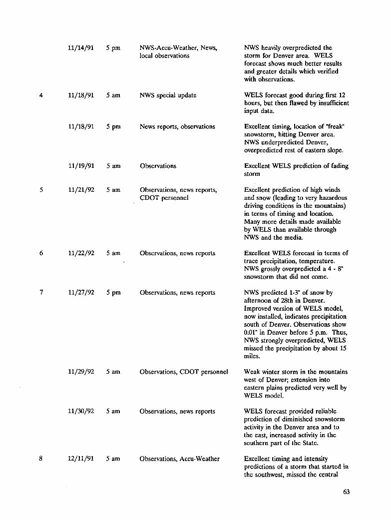
11/14/91 5 pm NWS-Accu-Weather, News, NWS heavily overpredicted thelocal observations storm for Denver area. WELS

forecast shows much better results

and greater details which verifiedwith observations.

4 11/18/91 5 am NWS special update WELS forecast good during first 12hours, but then flawed by insufficientinput data.

11/18/91 5 pm News reports, observations Excellent timing, location of "freak"snowstorm, hitting Denver area.NWS underpredicted Denver,overpredicted rest of eastern slope.

11/19/91 5 am Observations Excellent WELS prediction of fadingstorm

5 11/21/92 5 am Observations, news reports, Excellent prediction of high windsCDOT personnel and snow (leading to very hazardous

driving conditions in the mountains)in terms of timing and location.Many more details made availableby WELS than available throughNWS and the media.

6 11/22/92 5 am Observations, news reports Excellent WELS forecast in terms oftrace precipitation, temperature.NWS grossly overpredicted a 4 - 8"snowstorm that did not come.

7 11/27/92 5 pm Observations, news reports NWS predicted 1-3" of snow byafternoon of 28th in Denver.

Improved version of WELS model,now installed, indicates precipitationsouth of Denver. Observations show

0.01" in Denver before 5 p.m. Thus,NWS strongly overpredicted, WELSmissed the precipitation by about 15miles.

11/29/92 5 am Observations, CDOT personnel Weak winter storm in the mountainswest of Denver; extension intoeastern plains predicted very well byWELS model.

11/30/92 5 am Observations, news reports WELS forecast provided reliableprediction of diminished snowstormactivity in the Denver area and tothe east, increased activity in thesouthern part of the State.

8 12/11/91 5 am Observations, Accu-Weather Excellent timing and intensitypredictions of a storm that started inthe southwest, missed the central

63

mountains, and extended into the

northeastern plains. WELS forecastprovided much more detail thanNWS and media forecasts.

9 12/19/91 5 am NWS-Weather Brief, personal Details of WELS weather forecastobservations proved to be highly reliable, as

evident from personal trip report.Reliance in WELS forecast rather

than NWS forecast prompted theP.I. to choose mountain route to

Phoenix, AZ. Excellent forecast offlooding rains in Texas. NWS calledfor 30% chance of showers late in

the day, 3 -5" of snow by evening,which did not materialize.

12/20/91 5 am NWS-Weather Brief, personal Excellent forecast of drizzle and fogobservations, along eastern foothills, with rapid

clearing to follow. NWS calledagain for snow today, which did notmaterialize in the Denver area.

10 12/31/91 5 am NWS-Weather Brief, newspaper WELS caught the first half of adata rapidly moving system, with snow in

the west/central mountains, but

missed the shift to eastern slopesbefore 5 p.m.

12/31/91 5 pm NWS-Weather Brief, newspaper WELS now has good precipitationdata distribution for eastern Colorado

between 5 p.m. and 11 p.m. Decayof this weak storm by 11 p.m. also iswell predicted. NWS (WeatherBrief) delivered good forecast, butlacking details.

11 1/3/92 5 pm Data collected, but no forecast wasprepared, because no impact on

Greeley target area was anticipated.

10 1/6/92 5 am Excellent forecast of snow movinginto western and central mountains.

1/6/92 5 pm NWS-Weather Brief Good continuity with previous andsubsequent overlapping forecasts.

1/7/92 5 am NWS-Weather Brief Denver snow was underpredicted,but excellent forecast for all

surrounding regions.

1/7/92 5 pm NWS-Weather Brief Excellent continuity. Goodprediction of storm end. NWSforecasts were generally good, but

64

much less detailed, and tended tooverpredict snow in lower elevations.

13 1/11/92 5 am NWS-Weather Brief WELS forecast not attemptedbecause of insufficient data

reception.

1/12/92 5 am NWS-Weather Brief WELS provided excellent predictionof continuing blizzard conditionsover eastern plains, heavy snow inmountains. WELS gave moredetails than NWS, although NWSforecast called generic blizzardconditions correctly. WELS: Verygood portrayal of sharp horizontalgradients of precipitation east ofBoulder/Denver.

14 1/14/92 5 am NWS-Weather Brief Excellent WELS forecast ofrelatively dry storm with extremelycold temperatures and very strongwinds over eastern plains. Moredetails provided than available fromNWS. Observations indicate a

slightly wider extent of light snowthan shown by the forecast.

15 1/17/92 5 am NWS-Weather Brief This case confirmed that situationsin which nothing much happenscould be predicted well.

16 2/3/92 5 am NWS-Weather Brief NWS seemed to miss mountainsnow predicted by WELS. WELSshows considerable detail, but

seemed to over-predict PalmerRidge and Limon area.

Unfortunately, areas with highestpredicted precipitation do not havereporting stations.

17 2/10/92 5 am NWS Heavy snow advisory issued by NWSdid not materialize in WEI._forecast. No data were received to

verify predictions on this day.Reports from next day make nomention of any previous heavysnowfall.

18 2/11/92 5 am NWS-Weather Brief NWS forecast was correct, but verygeneric with no details. WELSforecast details verified well with

data from the few reporting stationsin the west.

2/12/92 5 am NWS-Weather Brief Only light snow showers expected in

65

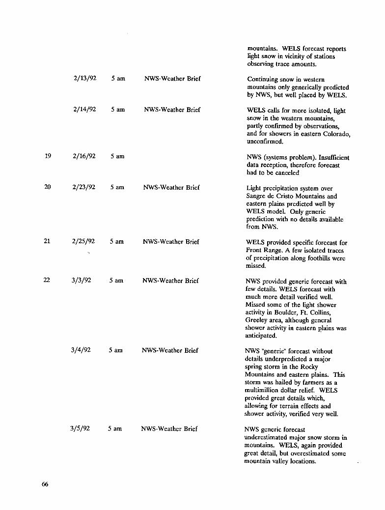
mountains. WELS forecast reportslight snow in vicinity of stationsobserving trace amounts.

2/13/92 5 am NWS-Weather Brief Continuing snow in westernmountains only generically predictedby NWS, but well placed by WELS.

2/14/92 5 am NWS-Weather Brief WELS calls for more isolated, lightsnow in the western mountains,

partly confirmed by observations,and for showers in eastern Colorado,unconfirmed.

19 2/16/92 5 am NWS (systems problem). Insufficientdata reception, therefore forecasthad to be canceled

20 2/23/92 5 am NWS-Weather Brief Light precipitation system overSangre de Cristo Mountains andeastern plains predicted well byWELS model. Only genericprediction with no details availablefrom NWS.

21 2/25/92 5 am NWS-Weather Brief WELS provided specific forecast forFront Range. A few isolated tracesof precipitation along foothills weremissed.

22 3/3/92 5 am NWS-Weather Brief NWS provided generic forecast withfew details. WELS forecast withmuch more detail verified well.

Missed some of the light showeractivity in Boulder, Ft. Collins,Greeley area, although generalshower activity in eastern plains wasanticipated.

3/4/92 5 am NWS-Weather Brief NWS "generic" forecast withoutdetails underpredicted a majorspring storm in the RockyMountains and eastern plains. This

storm was hailed by farmers as amultimillion dollar relief. WELS

provided great details which,allowing for terrain effects andshower activity, verified very well.

3/5/92 5 am NWS-Weather Brief NWS generic forecastunderestimated major snow storm inmountains. WELS, again providedgreat detail, but overestimated somemountain valley locations.

66

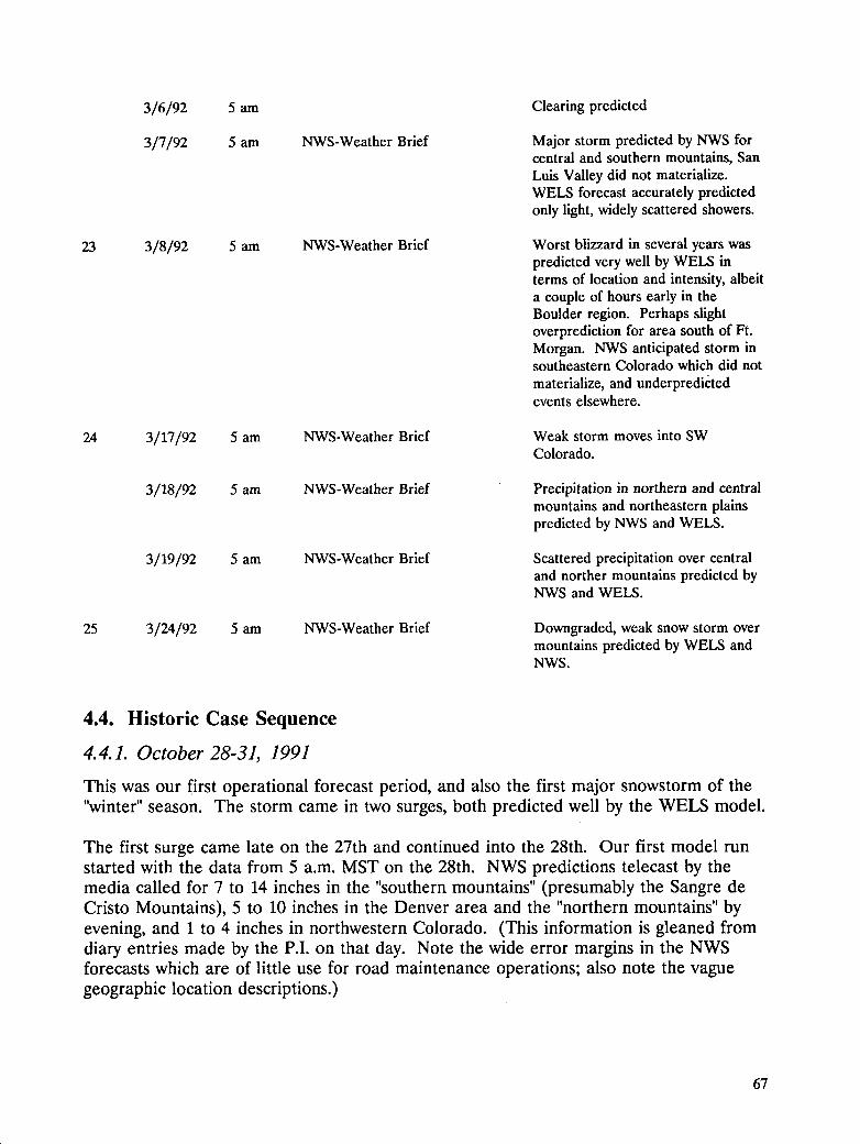
3/6/92 5 am Clearing predicted

3/7/92 5 am NWS-Weather Brief Major storm predicted by NWS forcentral and southern mountains, San

Luis Valley did not materialize.WELS forecast accurately predictedonly light, widely scattered showers.

23 3/8/92 5 am NWS-Weather Brief Worst blizzard in several years waspredicted very well by WELS interms of location and intensity, albeita couple of hours early in theBoulder region. Perhaps slight

overprediction for area south of Ft.Morgan. NWS anticipated storm insoutheastern Colorado which did not

materialize, and underpredictedevents elsewhere.

24 3/17/92 5 am NWS-Weather Brief Weak storm moves into SWColorado.

3/18/92 5 am NWS-Weather Brief Precipitation in northern and centralmountains and northeastern plainspredicted by NWS and WELS.

3/19/92 5 am NWS-Weather Brief Scattered precipitation over centraland norther mountains predicted byNWS and WELS.

25 3/24/92 5 am NWS-Weather Brief Downgraded, weak snow storm overmountains predicted by WELS andNWS.

4.4. Historic Case Sequence

4.4.1. October 28-31, 1991

This was our first operational forecast period, and also the first major snowstorm of the"winter" season. The storm came in two surges, both predicted well by the WELS model.

The first surge came late on the 27th and continued into the 28th. Our first model runstarted with the data from 5 a.m. MST on the 28th. NWS predictions telecast by themedia called for 7 to 14 inches in the "southern mountains" (presumably the Sangre deCristo Mountains), 5 to 10 inches in the Denver area and the "northern mountains" byevening, and 1 to 4 inches in northwestern Colorado. (This information is gleaned fromdiary entries made by the P.I. on that day. Note the wide error margins in the NWSforecasts which are of little use for road maintenance operations; also note the vaguegeographic location descriptions.)

67

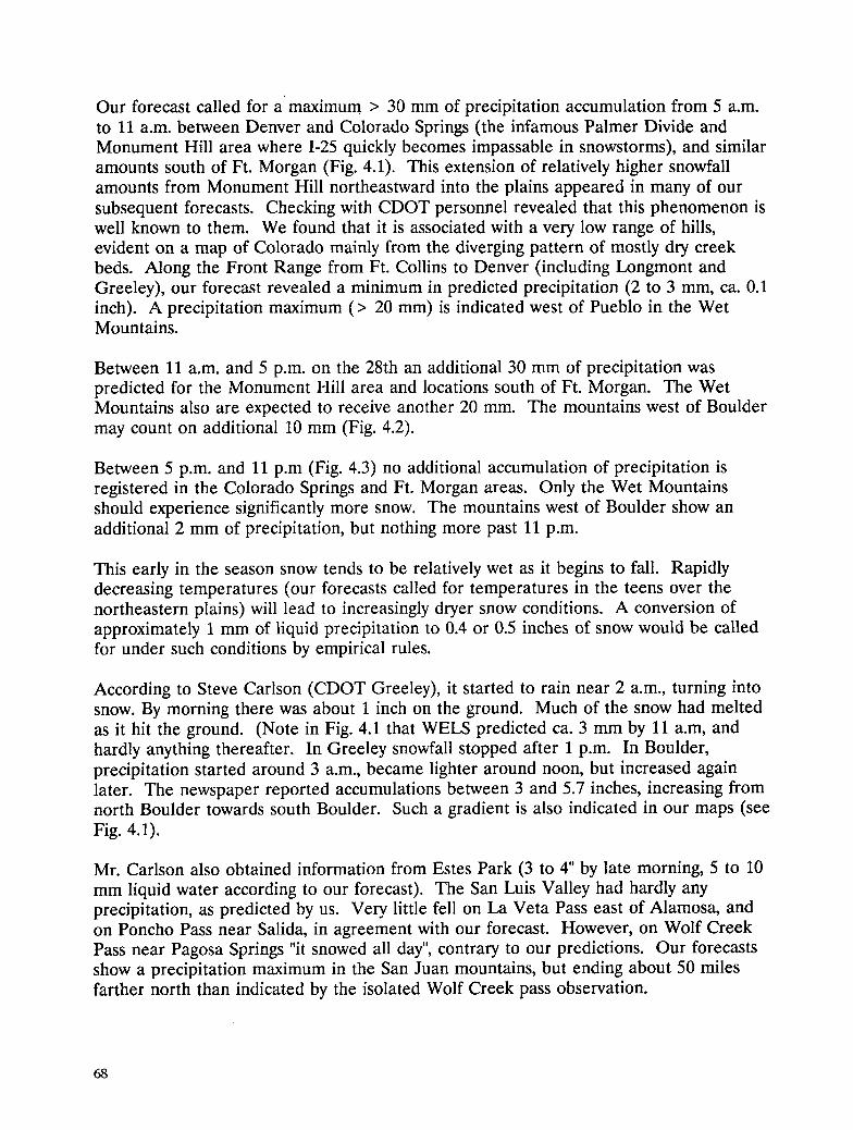
Our forecast called for a maximum > 30 mm of precipitation accumulation from 5 a.m.to 11 a.m. between Denver and Colorado Springs (the infamous Palmer Divide andMonument Hill area where 1-25 quickly becomes impassable in snowstorms), and similaramounts south of Ft. Morgan (Fig. 4.1). This extension of relatively higher snowfallamounts from Monument Hill northeastward into the plains appeared in many of oursubsequent forecasts. Checking with CDOT personnel revealed that this phenomenon iswell known to them. We found that it is associated with a very low range of hills,evident on a map of Colorado mainly from the diverging pattern of mostly dry creekbeds. Along the Front Range from Ft. Collins to Denver (including Longmont andGreeley), our forecast revealed a minimum in predicted precipitation (2 to 3 mm, ca. 0.1inch). A precipitation maximum (> 20 mm) is indicated west of Pueblo in the WetMountains.

Between 11 a.m. and 5 p.m. on the 28th an additional 30 mm of precipitation waspredicted for the Monument Hill area and locations south of Ft. Morgan. The WetMountains also are expected to receive another 20 ram. The mountains west of Bouldermay count on additional 10 mm (Fig. 4.2).

Between 5 p.m. and 11 p.m (Fig. 4.3) no additional accumulation of precipitation isregistered in the Colorado Springs and Ft. Morgan areas. Only the Wet Mountainsshould experience significantly more snow. The mountains west of Boulder show anadditional 2 mm of precipitation, but nothing more past 11 p.m.

This early in the season snow tends to be relatively wet as it begins to fall. Rapidlydecreasing temperatures (our forecasts called for temperatures in the teens over thenortheastern plains) will lead to increasingly dryer snow conditions. A conversion ofapproximately 1 mm of liquid precipitation to 0.4 or 0.5 inches of snow would be calledfor under such conditions by empirical rules.

According to Steve Carlson (CDOT Greeley), it started to rain near 2 a.m., turning intosnow. By morning there was about 1 inch on the ground. Much of the snow had meltedas it hit the ground. (Note in Fig. 4.1 that WELS predicted ca. 3 mm by 11 a.m, andhardly anything thereafter. In Greeley snowfall stopped after 1 p.m. In Boulder,precipitation started around 3 a.m., became lighter around noon, but increased againlater. The newspaper reported accumulations between 3 and 5.7 inches, increasing fromnorth Boulder towards south Boulder. Such a gradient is also indicated in our maps (seeFig. 4.1).

Mr. Carlson also obtained information from Estes Park (3 to 4" by late morning, 5 to 10mm liquid water according to our forecast). The San Luis Valley had hardly anyprecipitation, as predicted by us. Very little fell on La Veta Pass east of Alamosa, andon Poncho Pass near Salida, in agreement with our forecast. However, on Wolf CreekPass near Pagosa Springs "it snowed all day", contrary to our predictions. Our forecastsshow a precipitation maximum in the San Juan mountains, but ending about 50 milesfarther north than indicated by the isolated Wolf Creek pass observation.

68

The Boulder newspaper on the 29th published the following observations pertaining tothe preceding day, which can be compared with WELS predictions:

Station precipitation (liquid amount, inches)observed predicted

Akron missing > 1.2Alamosa none none

Colo. Spgs. 0.09 1.1Denver 0.17 0.2

Eagle 0.01 0.02Ft.Collins 0.05 0.08

Ft.Morgan missing 0.8Glcnwood Spgs. missing 0.02Grand Junction 0.37 0.2

Gunnison missing 0.4La Junta 0.07 0.1Lamar 0.05 0.12Pueblo none 1.2

Salida missing 0.2Trinidad none none

If these values can be trusted, we slightly over-predicted Colorado Springs, and alsoPueblo. (The heavy precipitation on Monument Hill north of Colorado Springs does notappear in any station reports, but was confirmed by news flashes about traffic pileups.)La Junta and Lamar appear with predictions of > 2 mm. It should be noted that Eagle,east of Glenwood Springs, showed a predicted amount on the order of less than 1 mm,whereas Grand Junction appears on our forecast map (Fig. 4.3) with 5 mm or 0.2 inches.Thus, it appears that even some of the detailed differences in precipitation patternsreflected in our forecasts and caused by terrain effects are matched by some of theobservations.

The abrupt end of the snowstorm in northeastern Colorado seemed to coincide with achange in wind patterns which went from slight up-slope conditions in the morning (Fig.4.1) to downslope conditions in the evening (Fig. 4.4). The downslope effects alsoshowed in the appearance of a slightly warmer tongue of air in the Denver - Boulder -Ft. Collins region, as compared to Ft. Morgan in the eastern plains.

The second storm surge started on October 29. The WELS forecast, again, was startedwith the 5 a.m. MST data. By 5 p.m. no precipitation was indicated anywhere in theState. By 5 a.m. only isolated precipitation appeared in northeastern Colorado. A datacheck revealed that several key stations from the western U.S. were missing from ourrecords. Therefore, this forecast could not be relied upon.

We started the model again with the data received at 5 p.m. This time, the 6-hourforecast for 11 p.m. showed light snow in the high mountains, ending just east of Greeley- Boulder -Denver (Fig. 4.5). By 5 a.m. (Fig. 4.6) snowfall was supposed to extend to theeastern plains, again with the Monument Hill area being hit hard (> 10"mm). Slightincreases in snow amounts were expected in northeastern Colorado and in the high partsof the western mountains by 11 a.m. on the 30th (Fig. 4.7), with practically nothing more

69

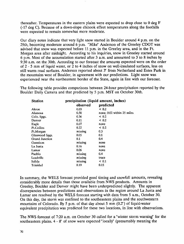
thereafter. Temperatures in the eastern plains were expected to drop close to 0 deg F(-17 deg C). Because of a down-slope chinook effect temperatures along the foothillswere expected to remain somewhat more moderate.

Our diary notes indicate that very light snow started in Boulder around 4 p.m. on the29th, becoming moderate around 6 p.m. "Mike" Anderson of the Greeley CDOT wasadvised that snow was expected before 11 p.m. in the Greeley area, and in the Ft.Morgan area after midnight. According to his inquiries, snow in Greeley started around6 p.m. Most of the accumulation started after 3 a.m. and amounted to 3 to 8 inches by9:30 a.m. on the 30th. According to our forecast the amounts expected were on the orderof 2 - 5 mm of liquid water, or 2 to 4 inches of snow on well-insulated surfaces, less onstill warm road surfaces. Anderson reported about 3" from Netherland and Estes Park inthe mountains west of Boulder, in agreement with our predictions. Light snow wasexperienced near the northeastern border of the State, again in line with our forecast.

The following table provides comparisons between 24-hour precipitation reported by theBoulder Daily Camera and that predicted by 5 p.m. MST on October 30th.

Station precipitation (liquid amount, inches)observed predicted

Akron 0.03 < 0.2Alamosa 0.50 none;0.02within25 milesColo. Spgs. 0.36 < 0.2Denver 0.11 < 0.2Eagle 0.07 noneFt.Collins 0.22 < 0.2Ft.Morgan missing 0.3GlenwoodSpgs. 0.05 0.1Grand Junction 0.1 0.4Gunnison missing noneLa Junta 0.16 noneLamar 0.06 nonePueblo missing 0.4Leadville missing traceSalida missing < 0.1Trinidad 0.19 0.15

In summary, the WELS forecast provided good timing and snowfall amourfts, revealingconsiderably more details than those available from NWS products. Amounts inGreeley, Boulder and Denver might have been underpredicted slightly. The apparentdiscrepancies between predictions and observations in the region around La Junta andLamar are resolved by the WELS forecast starting with data from 5 a.m., October 30.On this day, the storm was confined to the southeastern plains and the southwesternmountains of Colorado. By 5 p.m. of that day about 5 mm (0.2') of liquid-waterequivalent precipitation was predicted for these two locations, in line with observations.

The NWS forecast of 7:20 a.m. on October 30 called for a "winter storm warning' for thesoutheastern plains. 4 - 8' of snow were expected "locall3/' (presumably meaning the

70

Denver area), 1.5 ft in the foothills, and 1 - 4" on the "northeastern plateau" (whereverthat may be). Denver Channel 9 TV at 7 a.m. was more specific by calling for 8 - 12inches "west of I-2S', and 4 - 8 inches "east of I-2S'.

The media forecasts overestimated the storm system and its effects. It was a very fastmoving system. Such systems are notoriously difficult to predict, especially in theirup-slope effects on precipitation distributions. To keep track of them it will be necessaryto update weather forecasts every 12 hours as new radiosonde data are received.

4.4.2. November 6 - 8, 1991

WELS forecasts show strong northwesterly winds over mountains which should lead toblowing snow. Snowfall in excess of 20 mm (0.8") liquid water, representingapproximately 1 ft of snow, was predicted for the western mountains in the GrandJunction - Glenwood Springs - Montrose area, as well as in the mountains betweenLeadville and Salida. Light isolated rain showers were called for in the eastern plains, inagreement with the Channel 9 forecast. These showers did materialize in Akron,Denver, Ft. Collins, Ft. Morgan, according to Accu-Weather statistics. Glenwood Springsobserved 0.05" (predicted <0.1"), and Eagle observed 0.03" (predicted <0.1"). Newsreports in the evening indicated that 1-70 was closed across Vail Pass because of manyaccidents in blowing snow. This report is consistent with our high wind forecast. Snowhas been in this area from the last storm. Light, additional snow should be expected, asit has been forecast for a mountain region only 25 miles to the south. Light snowshowers observed in Denver were attributed to a "back door" cold front.

These frontal effects appeared in the WELS forecast initiated with data from 5 a.m. onNovember 7. While winds were still expected to be strong and from the northwest overthe mountains west of Boulder and Denver, winds east of Denver were predicted to belight early in the forecast period, picking up during the afternoon and night. WELSforecast light snow all along the Front Range from Boulder to the New Mexico border.According to morning newscasts, the high wind and drifting snow situation caused closureof Loveland Pass. Hazardous material transports, normally using the pass road, had to bediverted through the Eisenhower/Johnson tunnels. These tunnels, then, had to be closedfor other traffic, causing long delays.

4.4.3. November 14 - 17, 1991

The WELS forecast starting with data from 5 a.m., November 14, gave first indications ofsnow (0.2" to 0.4" liquid, equivalent to 2 to 6 " of snow) between 11 a.m. and 5 p.m. inthe mountains from Durango to Steamboat Springs. By 11 p.m. additional snow(equivalent to more than 1 ft in the Telluride region) was expected. Furthermore, theprecipitation pattern shifted to the east, now including the foothills west of Boulder/Ft.Collins, and west of Colorado Springs. Dave Fraser (CDOT Denver) was advised in thelate morning that with such a pattern usually we can also expect precipitation in theBoulder�Denver area. Because of the relatively warm temperatures in the plains, thisprecipitation should start out as rain. By 5 a.m. the storm was expected to involve all of

71

Colorado west of the foothills, with the exception of the Walsenburg/Alamosa area (Fig.4.8).

Because of the intensity and speed of this fast-moving weather system we also preparedforecasts using the 5 p.m. data of November 114as input to the WELS model. Fig. 4.9shows the precipitation predicted in the 12-hour period between 5 p.m. (forecast start)and 5 a.m. on November 15. The intensity of the storm over the western half ofColorado remained similar. The new forecast, however, indicated significant precipitationbetween Colorado Springs and Trinidad, along the eastern slopes of the Sangre de CristoMountains. Alamosa remained in a "dry island."

By 5 p.m. on November 15 the storm was expected to sweep into the northeastern plains(Figs. 4.10 and 4.11), curiously sparing the Denver - Boulder - Longmont area.Significant precipitation ( > 20 mm or 0.8" liquid, equivalent to approximately 8" of snow)were expected in the Monument Hill area south of Denver and in an area south of Ft.Morgan mentioned before as prone to snowstorms.

According to our diary notes, upslope clouds started to appear in Boulder around 4:30p.m., and rain started around 6:30 to 7 p.m. According to Steve Carlson (CDOTGreeley) by morning of November 15 Greeley had experienced light rain, turning intolight snow. Ft. Collins had about 1" of wet snow, the upper reaches of Poudre Canyonwest of Ft. Collins had about 5" of snow, in excellent agreement with our forecast. (Notethat we advised CDOT that we expected the precipitation pattern to reach a few milesfarther east than indicated in Fig. 4.8).

NWS and the media had predicted up to 1 ft of snow in Denver which, as showncorrectly by WELS, did not materialize. The snow stayed in higher elevations, inagreement with the WELS forecast. Vail Pass had to be closed again, as anticipatedfrom Fig. 4.8.

The P.I. had to drive from Boulder to Ft. Collins and back to Boulder in the evening ofNovember 15, relying on the WELS forecast in spite of dire travel advisories issued bythe media. Note that this trip coincided with the prediction shown in Fig. 4.10, whichshows the Boulder area to lie inside a "dry hole". Other than sporadic light drizzle andpatchy fog with a few snow flakes, no adverse weather was encountered.

72

The following table compares 24-hour precipitation amounts predicted by 5 p.m. onNovember 5 with statistical data published in the Boulder Daily Camera in the morningof November 16, presumably dating to the evening before.

Station precipitation (liquid amount, inches)observed predicted

Akron none 0.3

Alamosa 0.1 none; 0.02 within 15 milesColo. Spgs. 0.14 0.4Denver 0.15 Trace

Eagle 0.09 0.4Ft.Collins 0.31 0.2

Ft.Morgan 0.09 0.4Glenwood Spgs. 0.12 0.8Grand Junction 0.6 1.2

Gunnison missing 1.6La Junta 0.03 <0.1Lamar none noneLeadville 0.05 0.2Pueblo 0.04 1.2

Salida m!ssing < 0.1Trinidad 0.14 0.8

Newspaper statistics also show Boulder to have received 1.5" of snow by 6 p.m. onNovember 15.

The WELS forecast issued from the 5 a.m. data of November 16 showed the snowstorm

moved into eastern Colorado, dying out after 11 p.m.

4.4.4. November 18- 19, 1991

This storm followed on the heels of the previous one. The predictions derived from the5 a.m. data on November 18 show the storm starting in southwestern Colorado, coveringmost of western Colorado by 5 p.m., but then breaking up. This fact made us suspiciousabout our input data. Indeed, several key stations were missing.

NWS issued a special update in the late afternoon, calling for 4 -6" of snow in theBoulder-Denver area within the next few hours. This snow was not evident from the 5

a.m. forecast run, but was excellently revealed in terms of location and timing in theforecast run using the 5 p.m. data.

Precipitation in Boulder started around 4 p.m. Boulder received about 2" until nextmorning out of this storm. The Denver airport reported 13" on the runways as of 7:30a.m. North of Boulder there was little snow accumulation. Ft. Collins only had about1/2 to 1" of snow during the night.

The WELS forecast starting with the 5 a.m. data of November 19 showed continuinglight snow in Denver between 5 a.m. and 11 a.m., nothing more thereafter.

73

4. 4. 5. November 21, 1991

According to our diary notes, the NWS predicted partly cloudy conditions statewide,except for Trinidad and Glenwood Springs calling for clear skies. Denver was to expectpartly cloudy conditions with highs near 45 and a low of 28 degrees. The forecast for thesubsequent day called for cloudy, with a high near 44 and a low in the twenties.

The WELS model indicates precipitation in the region of Grand Junction and GlenwoodSprings, decreasing during the afternoon, but flaring up again after midnight when snowis also expected over the Continental Divide west of Boulder and in the northern part ofthe Sangre de Cristo Mountains. From past experience with similar forecast patterns wecalled for a chance of rain to spill over into the Denver/Boulder region between 5 p.m.and 11 p.m. The model did extremely well in predicting strong Chinook wind conditionsalong the Front Range between Ft. Collins and Colorado Springs. Strongest winds near28 m/sec (62 mph) were expected in the Boulder area by 11 a.m., easing back to about45 mph by evening, but increasing to about 50 mph during the night. In contrast,Greeley was expected to have only light winds, even though it is only about 40 km (25miles) to the east of the mountains. This wind forecast was confirmed by CDOTpersonnel in Greeley.

Accu-Weather statistics in the Boulder Daily Camera indicated 0.01" of precipitation inEagle (east of Glenwood Springs), in agreement with our forecast. Boulder had verylight drizzle around 5 p.m. Denver reported very light rain around 10 p.m., whichstopped soon after it started. Vail Pass had the chain law in effect. Loveland Pass hadto be closed because of a semi-truck accident. According to the WELS forecast, theselocations are within the predicted region of heaviest snow fall (> 10 mm liquidequivalent, or > 4" snow) and winds near 50 mph near the Continental Divide.

Media forecasts broadcast in the evening expected up to 4" of snow tonight. Snowadvisories were issued for 1-70 west of Denver. Rain was expected east of Denver.

4. 4. 6. November 22 - 23, 1991

Recall the NWS and media predictions calling for 4" of snow in the Denver area. Noneof it came, as anticipated by WELS. The NWS forecast issued this morning, again, callsfor snow today and tomorrow. Temperature high in the thirties for today, a low in the

twenties, and a high of 35 for tomorrow is expected.

In contrast, the WELS model predicted continuing light snow in the mountains west ofBoulder/Denver (ca 5 mm liquid, or 2" of snow in 6 hours). Light snow ( < 1" of snowin 6 hours) was also expected in the Sangre de Cristo mountains southwest of ColoradoSprings, and in an area between Montrose, Aspen and Glenwood Springs. Snowfall inthese areas was expected to diminish into the afternoon and night. WELS temperaturepredictions call for a decreasing trend, starting in the mid twenties and dropping into theteens, lower than the ones anticipated by NWS.

74

Our weather diary shows a light snow flurry in Boulder around 1 p.m., but heavier cloudswith virga over the foothills, with patches of blue sky off and on appearing over themountains. In the late afternoon, again a few light snow flurries rendered the streetswet, but caused no accumulation. However, in the Denver area, these light flurries,together with the cold temperature invasion, caused major traffic problems due to ice on1-25. Traces of precipitation were reported by 5 p.m. from Denver, Glenwood Springs,Grand Junction, La Junta, Pueblo, and Trinidad.

Data transmission from the National Meteorological Center (NMC) went down today,therefore no evening data could be received. The NOAA offices in Boulder seemed tohave been affected in the same way.

4.4. 7. November 27 - December 1, 1991

Beginning with this case a significantly improved version of the nested grid model wasput into operation. It mainly affected the way in which solutions were found for thePoisson equation which accounts for the effects of terrain on the wind field.

The WELS forecasts prepared from the data of 27 November, 5 a.m. show a lightprecipitation system moving into the mountainous areas of northwestern Colorado.Starting the forecasts with the data from 5 p.m. indicate this precipitation system to beeven weaker at 5 a.m. on the 28th, with first indications of precipitation by 11 a.m. alsoappearing west and north of Colorado Springs• By 5 p.m. on November 28 the WELSmodel predicted snow over most of the central Colorado mountains. The precipitationactivity was expected to spill onto the eastern slopes in the Monument Hill area betweenDenver and Colorado Springs (Fig. 4.12).

The morning forecast on Channel 9 calls for sleet in the afternoon, with snowaccumulation from 1 to 3". Weather statistics published in the Boulder Daily Camera for5 p.m. on the 28th indicate 0.01" of precipitation in Denver and 0.03" in Ft. Collins, muchless than what was indicated in the earlier warnings.

The next forecast, prepared from the data of November 29, 5 a.m., shows snow by 11a.m. in Denver, Boulder, and in the mountains to the west (Fig. 4.13). By 5 p.m. aprecipitation tongue was expected to extend into the eastern plains southwest of Denver.Light snow was expected to continue in the region south of Ft. Morgan until morning,while the Denver/Boulder area was expected to clear already after 11 a.m.

Our diary notes indicate snow in Boulder starting around 6 a.m., ending around 11 a.m.with an accumulation of 1 to 2", but melting on road surfaces. (Fig. 4.13 indicates 2 mmof liquid-equivalent precipitation or about 1" of snow for Boulder by 11 a.m., nothingthereafter.). CDOT personnel in Greeley reported that snow was observed south of Ft.Morgan to Last Chance (the limits of their District's responsibility), in excellentagreement with our forecast. News media reported 3" of snow south of Ft. Morgan, ascompared to 15 mm (0•6") liquid, or approximately 6" of snow, predicted by WELS asupper limit.

75

The WELS forecast from data received on November 30, 5 a.m., indicates snow fromBoulder to Colorado Springs until 11 a.m., with maximum amounts near 2 mm liquid, or< 1" of snow. Small amounts were also predicted by noon for the areas around Puebloand Lamar. Data published in the newspaper indicate 0.01" (liquid equivalent) in Pueblo,0.10 in Denver, traces in Colorado Springs and Ft. Collins, in excellent agreement withthe WELS prediction. Boulder reported 3" of snow, quitting around 6 a.m. This snowwas missed by a few miles in yesterday's and today's forecast.

Between 5 p.m. on November 30 and 5 a.m. on December 1, WELS predicted significantsnow for the Red Mountain Pass area north of Durango and for the eastern foothillsbetween Pueblo and Trinidad. According to observations from Alamosa and Trinidad,some of this storm activity may have arrived already before 5 p.m. on November 30.

4.4.8. December 11 - 12, 1991

This case provides a classic example of a rapidly moving storm, associated with strongChinook winds over the Continental Divide west of Denver. According to our notes, theNWS forecast in the morning of December 11 called for snow in the Grand Valley(around Grand Junction) and in the southwest corner of the State, possible snow flurriesin metropolitan Denver. The Denver forecast advised of a 20% chance of rain mixedwith snow, highs in the upper thirties, a 30% chance of snow showers tonight, decreasingafter midnight. Lows in the 20 to 25 deg F range. The Channel 9 forecast warned of 8"of snow in the San Juan mountains and in the foothills west of Trinidad.

The WELS forecast showed light snow in the southeastern corner of Utah before 11 a.m.on December 11, none in Colorado. By 5 p.m. (Fig. 4.14) approximately 10 mm (0.4"liquid) were expected in the Grand Junction area, extending all the way to GlenwoodSprings. Similar amounts were expected between Durango and Pagosa Springs in thesouthwestern part of the State. Trinidad, Pueblo, La Junta and Lamar encompassedother regions with predicted precipitation. The following table gives comparisons

76

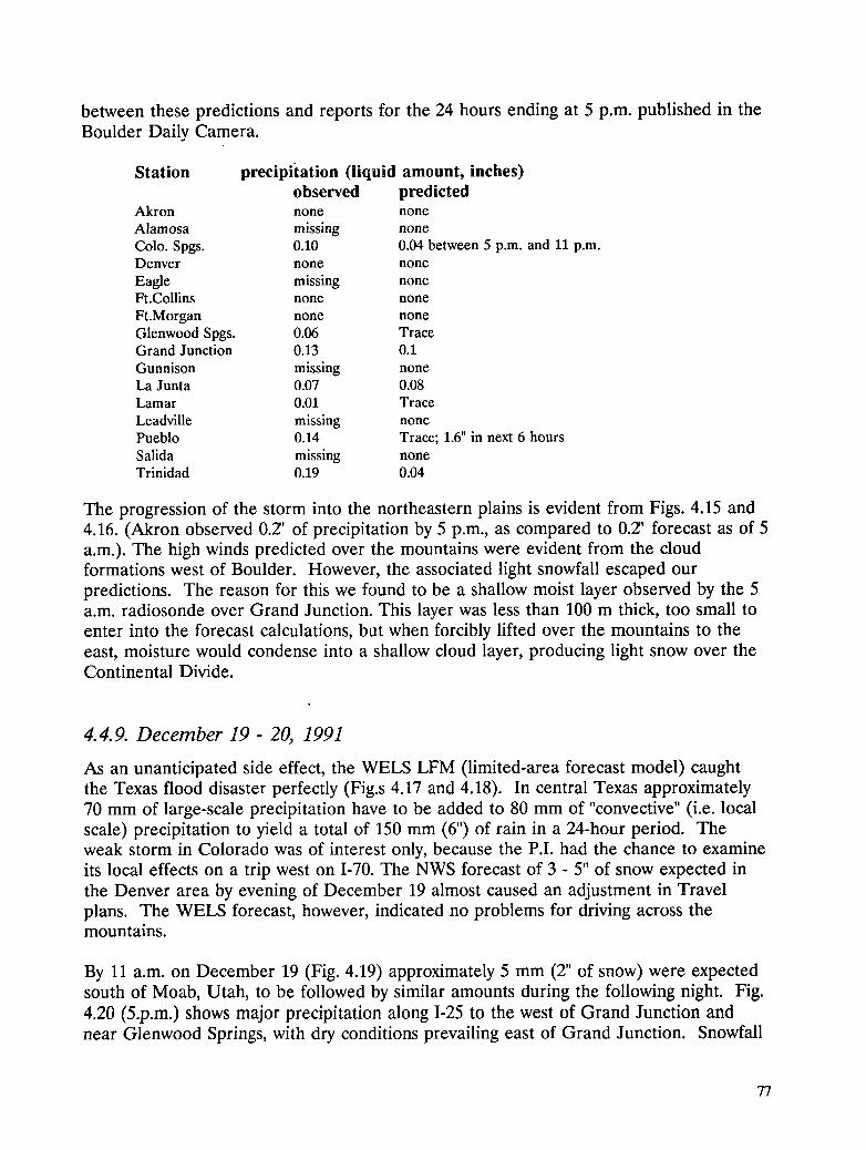
between these predictions and reports for the 24 hours ending at 5 p.m. published in theBoulder Daily Camera.

Station precipitation (liquid amount, inches)observed predicted

Akron none none

Alamosa missing noneColo. Spgs. 0.10 0.04 between 5 p.m. and 11 p.m.Denver none none

Eagle missing noneFt.Collins none none

Ft.Morgan none noneGlenwood Spgs. 0.06 TraceGrand Junction 0.13 0.1

Gunnison missing noneLa Junta 0.07 0.08Lamar 0.01 Trace

Leadville missing nonePueblo 0.14 Trace; 1.6" in next 6 hours

Salida missing noneTrinidad 0.19 0.04

The progression of the storm into the northeastern plains is evident from Figs. 4.15 and4.16. (Akron observed 0.2' of precipitation by 5 p.m., as compared to 0.2' forecast as of 5a.m.). The high winds predicted over the mountains were evident from the cloudformations west of Boulder. However, the associated light snowfall escaped ourpredictions. The reason for this we found to be a shallow moist layer observed by the 5a.m. radiosonde over Grand Junction. This layer was less than 100 m thick, too small toenter into the forecast calculations, but when forcibly lifted over the mountains to theeast, moisture would condense into a shallow cloud layer, producing light snow over theContinental Divide.

4.4.9. December 19 - 20, 1991

As an unanticipated side effect, the WELS LFM (limited-area forecast model) caughtthe Texas flood disaster perfectly (Fig.s 4.17 and 4.18). In central Texas approximately70 mm of large-scale precipitation have to be added to 80 mm of "convective" (i.e. localscale) precipitation to yield a total of 150 mm (6") of rain in a 24-hour period. Theweak storm in Colorado was of interest only, because the P.I. had the chance to examineits local effects on a trip west on 1-70. The NWS forecast of 3 - 5" of snow expected inthe Denver area by evening of December 19 almost caused an adjustment in Travelplans. The WELS forecast, however, indicated no problems for driving across themountains.

By 11 a.m. on December 19 (Fig. 4.19) approximately 5 mm (2" of snow) were expectedsouth of Moab, Utah, to be followed by similar amounts during the following night. Fig.4.20 (5.p.m.) shows major precipitation along 1-25 to the west of Grand Junction andnear Glenwood Springs, with dry conditions prevailing east of Grand Junction. Snowfall

77

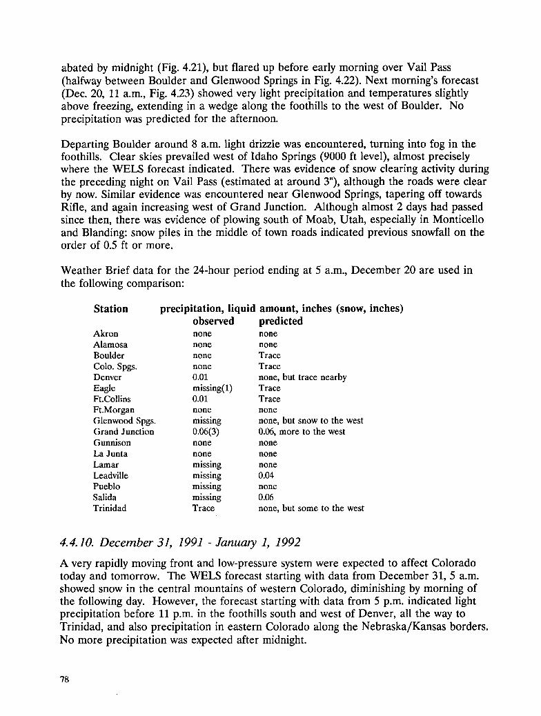
abated by midnight (Fig. 4.21), but flared up before early morning over Vail Pass(halfway between Boulder and Glenwood Springs in Fig. 4.22). Next morning's forecast(Dec. 20, 11 a.m., Fig. 4.23) showed very light precipitation and temperatures slightlyabove freezing, extending in a wedge along the foothills to the west of Boulder. Noprecipitation was predicted for the afternoon.

Departing Boulder around 8 a.m. light drizzle was encountered, turning into fog in thefoothills. Clear skies prevailed west of Idaho Springs (9000 ft level), almost preciselywhere the WELS forecast indicated. There was evidence of snow clearing activity duringthe preceding night on Vail Pass (estimated at around 3"), although the roads were clearby now. Similar evidence was encountered near Glenwood Springs, tapering off towardsRifle, and again increasing west of Grand Junction. Although almost 2 days had passedsince then, there was evidence of plowing south of Moab, Utah, especially in Monticelloand Blanding: snow piles in the middle of town roads indicated previous snowfall on theorder of 0.5 ft or more.

Weather Brief data for the 24-hour period ending at 5 a.m., December 20 are used inthe following comparison:

Station precipitation, liquid amount, inches (snow, inches)observed predicted

Akron none noneAlamosa none noneBoulder none Trace

Colo. Spgs. none TraceDenver 0.01 none, but trace nearbyEagle missing(l) TraceFt.Collins 0.01 Trace

Ft.Morgan none none

Glenwood Spgs. missing none, but snow to the westGrand Junction 0.06(3) 0.06, more to the westGunnison none noneLa Junta none none

Lamar missing noneLeadville missing 0.04Pueblo missing noneSalida missing 0.06Trinidad Trace none, but some to the west

4.4.10. December 31, 1991 -January L 1992

A very rapidly moving front and low-pressure system were expected to affect Coloradotoday and tomorrow. The WELS forecast starting with data from December 31, 5 a.m.showed snow in the central mountains of western Colorado, diminishing by morning ofthe following day. However, the forecast starting with data from 5 p.m. indicated lightprecipitation before 11 p.m. in the foothills south and west of Denver, all the way toTrinidad, and also precipitation in eastern Colorado along the Nebraska/Kansas borders.No more precipitation was expected after midnight.

78

4.4.11. January 3, 1992

According to Weather Brief, snow was expected in mountains near Aspen. Datawere received, but no forecast was prepared by WELS, because no impact wasanticipated for the Boulder/Greeley area.

4.4.12. January 6 - 8, 1992

NWS (as distributed by Weather Brief) expected snow beginning this afternoon in themountains of western Colorado. Accumulation in the southwestern mountains was

expected to be heavy, 10 - 15". Heavy accumulation expected in northern and centralMountains tomorrow. 2 - 5" in lower elevations tonight, with an additional 1 -4" possibletomorrow. Gusty winds with areas of blowing and drifting snow in the mountains.

The WELS forecast, starting with 5 a.m., January 6, showed strong southwesterly windsof 40 mph over the western mountains. Strong southwesterly to southerly winds werealso predicted over the eastern plains. Snow accumulation at the rate of more than 5mm liquid per hours (1 to 2" per six hours) is predicted until tomorrow morning over thesouthwestern and western mountains, especially in the Red Mountain area and themountain regions to the north and south of Glenwood Springs. For the eastern plainsisolated shower activity is predicted, mainly centered on the region between ColoradoSprings, Pueblo and Limon.

The forecast started at 5 p.m. on January 6 showed similar features in the precipitationdistribution, with precipitation also extending into the Steamboat Springs area ofnorthwestern Colorado. According to this forecast sequence, more snowfall wasexpected in the Red Mountain area north of Durango by 5 a.m.

NWS called for winter storm warning for north central and northeastern Colorado, withblizzard conditions over portions of the Front Range and Palmer Divide. 6 - 14" of snowexpected in lower elevations, up to 2 ft in mountains and foothills.

In the forecast starting with 5 a.m. on January 7, snow was expected in the mountainswest of Boulder, becoming heavy in the Monument Hill area south and east of Denver(up to 20 mm or 0.8" liquid by 11 a.m., which would translate to about 8" of snow (Fig.4.24). Strong northerly winds near 30 mph should give rise to blizzard conditions. Theregion around Boulder was expected to receive only light snow. Snowfall in theBoulder/Denver area was expected to decrease in the afternoon (Fig. 4.25). However,precipitation was expected to continue in eastern Colorado and in the westernmountains.

Another forecast run, starting with 5 p.m. on January 7 showed a resurgence of thestorm, mainly along the foothills south of Colorado Springs and in the plains east ofDenver (Figs. 4.26, 4.27, 4.28). The Sangre de Cristo and San Juan Mountains also wereexpected to receive significant precipitation.

79

The forecast starting at 5 a.m. on January 8 finally signalled the end of the storm with noprecipitation in sight.

Verification for the forecasts ending on 7 January, 8 a.m.:

Station precipitation, liquid amount, inches (snow, inches)observed predicted

Akron Trace none, but scattered showers possibleAlamosa 0.08 none, but significant precip starting 10 mi westBoulder Trace none, but showers possibleColo. Spgs. Trace TraceCraig 0.18 0.04Denver 0.02 none, but showers possibleEagle Trace TraceFt.Collins none none

Ft.Morgan 0.02 none, but showers possibleGlenwood Spgs. missing 0.08

Grand Junction 0.15(2) 0.12Gunnison missing TraceLa Junta missing none, but showers possibleLamar missing none, but showers possibleLeadville missing Trace, more to the southPueblo missing none, but showers possibleSalida missing TraceTrinidad 0.2 none, but showers possible

Verification of the forecasts ending January 8, 5 a.m.:

Station precipitation, liquid amount, inches (snow, inches)observed predicted

Akron 0.37(8) 0.4 (> 4)

Alamosa none none, but precip in near mountainsBoulder 0.03 0.01 - 0.05

Colo. Spgs. 0.03 0.4Craig 0.01 0.9Denver 0.68 0.08, but heavy all around (see Ft.Morgan)Eagle Trace TraceFt.Collins 0.46 0.04, but heavy to west and northwestFt.Morgan missing 0.6Glenwood Spgs. missing 0.2Grand Junction Trace 0.1Gunnison none 0.15La Junta 0.03 none

Lamar missing noneLeadville missing 0.2Pueblo Trace 0.1

Salida missing TraceTrinidad none none, but precip in mountains to west

80

4.4.13. January 11 - 13, 1992

Under the current testing conditions, WELS was not set up to run 24-hour and weekendshifts. This storm developed over the weekend (Saturday Jan.ll, Sunday Jan. 12). As aconsequence, a data reception problem, probably due to snow accumulation on theantenna, remained unchecked. Due to poor data quality, the forecast starting with 5a.m., January 11, showed no precipitation in Colorado, even though light rain showerswere observed around 8 p.m. over the southern foothills. By 5:50 a.m. much of easternColorado experienced snow. Heavy snow was reported from Limon on south, falling at arate of 2 - 3" per hour. All roads out of Limon had to be closed. Light snow wasreported from western valleys.

The WELS forecast starting at 5 a.m., Sunday January 12 showed strong northerly windsover eastern Colorado in excess of 30 mph, in line with Observation. By 11 a.m. PalmerRidge/Monument Hill show precipitation close to 20 mm (0.8"), and almost 10 mm (0.4")were expected north of Limon. Denver and Boulder were expected to receive 5 mm(0.2"). The mountains west of Boulder were expected to receive in excess of 10 mm (4 to6" of snow in 6 hours). Precipitation was forecast to extend as far south as Pueblo. By 5p.m. strong northerly winds, now up to 40 mph, were expected to continue over theplains. Another 10 mm of precipitation were predicted in the Monument Hill area and inthe mountains west of Boulder and Denver, as well as in the Wet Mountains and Sangrede Cristo mountains west of Pueblo. The edge of the predicted precipitation lineextends from Pueblo to Limon, signalling the end of snowfall there. By 11 p.m. another10 mm were expected along the whole Front Range of the Rocky Mountains from theWyoming border to Trinidad. By 5 a.m. light snow is indicated again over most ofeastern Colorado, with 6-hour accumulations of more than 10 mm liquid-equivalent (4 -6" of snow) over Monument Hill and an area between Limon and Fort Morgan.

81

NWS data received from Weather Brief may serve to verify this forecast.

Station precipitation, liquid amount, inches (snow, inches)

observed predictedAkron 0.23(8) <0.1, much more to southAiamosa missing none, but precip in near mountainsBoulder 0.12 0.16

Colo. Spgs. 0.01 0.8Craig none 0.15Denver 0.18 0.2Eagle Trace TraceFt.Collins 0.13 Trace

Ft.Morgan 0.04 none, but heavy a few miles southGlenwood Springs missing noneGrand Junction Trace noneGreeley 0.18 none, but snow 20 miles to eastGunnison missing noneLa Junta 0.1 0.02

Lamar missing 0.08Leadville missing none, but heavy a few miles to eastLimon 0.11 0.06Longmont 0.02 0.04Pueblo Trace 0.5

Salida missing noneTrinidad 0.07 0.2

4.4.14. January 14 - 15, 1992

The NWS forecast by Weather Brief issued at 3:40 p.m. Tuesday January 14 states:

"Turning sharply colder and windy from north to south tonight with snow likely over

northeast and a chance of snow southeast. Areas of blowing and drifting snow northeast

with extremely cold wind chill temperatures. A chance of light snow early Wednesday in

the southeast, otherwise becoming sunny ..... Lows tonight 5 below to 10 above zeronortheast with 5 to 15 southeast.

The WELS forecast produced with the 5 a.m. data on January 14 indicates northwesterlywinds near 50 mph over the eastern plains at 11 a.m., turning into a northerly direction

by 5 p.m., and remaining strong all afternoon and night. By 11 a.m. a weak precipitation

system appeared in western Colorado, centered between Grand Junction and Montrose.

By 5 p.m. the system weakened and became disorganized. By 11 p.m. the area between

Boulder and Colorado Springs indicated light precipitation, extending into the easternplains. (Our weather notes indicated that light snow started in Boulder around 6:30

p.m., in agreement with the forecast.) This pattern weakened by 5 a.m. on January 15.Temperatures in the Boulder/Denver area were predicted to drop from near freezing in

the morning of the 14th to near zero F, or slightly below, by 5 a.m. on the 15th, in

agreement with observations. The southeastern part of the State was expected to stay

warmer by about 10 deg F.

82

Observations for the 24-hour period ending January 15, 5 a.m. compare as follows:

Station precipitation, liquid amount, inches (snow, inches)observed predicted

Akron Trace none, but trace possibleAlamosa missing noneBoulder 0.01 Trace

Colo. Spgs. 0.02 TraceCraig missing 0.04Denver 0.16 0.12

Eagle Missing TraceFt.Collins none none

Ft.Morgan none none, but measurable a few miles southGlenwood Springs missing TraceGrand Junction Trace 0.03

Greeley none noneGunnison missing noneLa Junta 0.07 none

Lamar missing noneLeadville missing noneLimon 0.01 none, but light 20 mi to NWLongmont 0.01 nonePueblo 0.04 none, but more in mountains to W

Salida missing noneTrinidad 0.13 none, but more in mountains to NW

4.4.15. January 17, 1992

NWS (Weather Brief) called for widely scattered snow showers mainly over themountains. This is also what the WELS forecast starting at 5 a.m., January 17, indicates.Winds of > 30 mph were predicted for high mountain ranges. Lower elevations wereexpected to have only light winds.

4. 4.16. February 3 - 4, 1992

The NWS forecast for Colorado issued at 3:15 a.m. by Weather Brief for today andtonight calls for "mostly cloudy east and mountains, partly cloudy west. Rain and mixedrain and snow likely eastern border today, and a chance of rain and snow showerselsewhere in the east. Decreasing clouds Tuesday (tomorrow). Colder in the eastthrough Tuesday."

In the WELS forecast issued with 5 a.m. data, February 3, showed major precipitationalong the main mountain range west of Boulder and Denver, the Sangre de CristoMountains west of Pueblo and Trinidad, the Red Mountain area north of Durango, andthe mountains north of Glenwood Springs. Monument Hill south of Denver extended ahigh precipitation "finger" into the region between Ft. Morgan and Limon. Lightprecipitation (rain) was also expected along the Kansas border. During the night theprecipitation over the eastern plains was expected to let up. Most of the snow wasexpected to occur during the night along a line from north of Limon, to Colorado

83

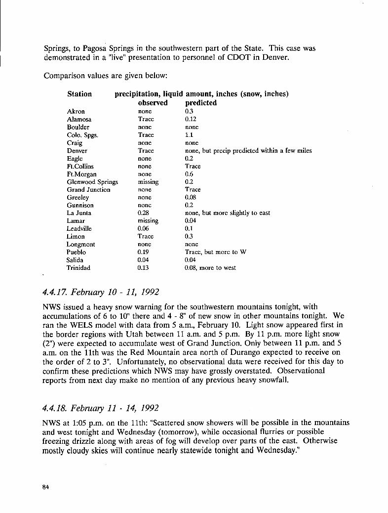
Springs, to Pagosa Springs in the southwestern part of the State. This case wasdemonstrated in a "live" presentation to personnel of CDOT in Denver.

Comparison values are given below:

Station precipitation, liquid amount, inches (snow, inches)observed predicted

Akron none 0.3Alamosa Trace 0.12Boulder none none

Colo. Spgs. Trace 1.1Craig none noneDenver Trace none, but precip predicted within a few milesEagle none 0.2Ft.Collins none Trace

Ft.Morgan none 0.6Glenwood Springs missing 0.2Grand Junction none Trace

Greeley none 0.08Gunnison none 0.2

La Junta 0.28 none, but more slightly to eastLamar missing 0.04Leadville 0.06 0.1Limon Trace 0.3

Longmont none nonePueblo 0.19 Trace, but more to WSalida 0.04 0.04

Trinidad 0.13 0.08, more to west

4.4.17. February 10 - 11, 1992

NWS issued a heavy snow warning for the southwestern mountains tonight, withaccumulations of 6 to 10" there and 4 - 8" of new snow in other mountains tonight. Weran the WELS model with data from 5 a.m., February 10. Light snow appeared first inthe border regions with Utah between 11 a.m. and 5 p.m. By 11 p.m. more light snow(2") were expected to accumulate west of Grand Junction. Only between 11 p.m. and 5a.m. on the llth was the Red Mountain area north of Durango expected to receive onthe order of 2 to 3". Unfortunately, no observational data were received for this day toconfirm these predictions which NWS may have grossly overstated. Observationalreports from next day make no mention of any previous heavy snowfall.

4.4.18. February 11 - 14, 1992

NWS at 1:05 p.m. on the llth: "Scattered snow showers will be possible in the mountainsand west tonight and Wednesday (tomorrow), while occasional flurries or possiblefreezing drizzle along with areas of fog will develop over parts of the east. Otherwisemostly cloudy skies will continue nearly statewide tonight and Wednesday."

84

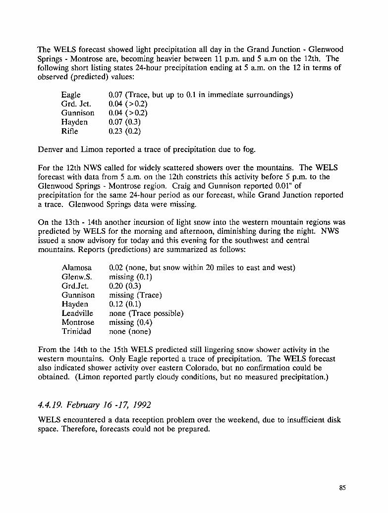
The WELS forecast showed light precipitation all day in the Grand Junction - GlenwoodSprings - Montrose are, becoming heavier between 11 p.m. and 5 a.m on the 12th. Thefollowing short listing states 24-hour precipitation ending at 5 a.m. on the 12 in terms ofobserved (predicted) values:

Eagle 0.07 (Trace, but up to 0.1 in immediate surroundings)Grd. Jct. 0.04 (> 0.2)Gunnison 0.04 ( > 0.2)Hayden 0.07 (0.3)Rifle 0.23 (0.2)

Denver and Limon reported a trace of precipitation due to fog.

For the 12th NWS called for widely scattered showers over the mountains. The WELSforecast with data from 5 a.m. on the 12th constricts this activity before 5 p.m. to theGlenwood Springs - Montrose region. Craig and Gunnison reported 0.01" ofprecipitation for the same 24-hour period as our forecast, while Grand Junction reporteda trace. Glenwood Springs data were missing.

On the 13th - 14th another incursion of light snow into the western mountain regions waspredicted by WELS for the morning and afternoon, diminishing during the night. NWSissued a snow advisory for today and this evening for the southwest and centralmountains. Reports (predictions) are summarized as follows:

Alamosa 0.02 (none, but snow within 20 miles to east and west)Glenw.S. missing (0.1)Grd.Jct. 0.20 (0.3)Gunnison missing (Trace)Hayden 0.12 (0.1)Leadville none (Trace possible)Montrose missing (0.4)Trinidad none (none)

From the 14th to the 15th WELS predicted still lingering snow shower activity in thewestern mountains. Only Eagle reported a trace of precipitation. The WELS forecastalso indicated shower activity over eastern Colorado, but no confirmation could beobtained. (Limon reported partly cloudy conditions, but no measured precipitation.)

4.4.19. February 16 -17, 1992

WELS encountered a data reception problem over the weekend, due to insufficient diskspace. Therefore, forecasts could not be prepared.

85

4.4.20. February 23 -24, 1992

The NWS forecast at 1:05 p.m. on the 23rd called for "gusty north winds with snow in themountains and rain and snow at some lower elevations."

The WELS forecast with 5 a.m. data from the 23rd indicates by 11 a.m. precipitation upto 10 mm over the mountains west of Colorado Springs, extending southward to Trinidadwith diminishing amounts. A region between Ft. Morgan and Limon also showed up to10 mm, mostly as rain. Similar amounts were to be expected during the next 6 hoursuntil 5 p.m., with precipitation spreading to the Kansas border. By 11 p.m. the mountainsnows were expected to subside, except for the Monument Hill region. Moreprecipitation was expected in the SW corner of the State. By 5 a.m. only isolatedpockets of precipitation were left. A comparison between observed (predicted)precipitation is given as follows:

Akron 0.25 (0.1, but more to south)Boulder none (none)Colo.Sp. 0.02 (0.2)Denver none (Trace)Ft.Morgan 0.01 (<0.1)La Junta Trace (none, but more 20 miles to east)Limon 0.03 (0.1)Trinidad Trace (0.2)

4.4.21. February 25 -26, 1992

NWS called for snow to continue in parts of the northern and central mountains. TheWELS forecast between 5 a.m. and 11 a.m. showed snow in a narrow band along thewhole Front Range between the Wyoming and New Mexico borders. Heaviestaccumulations (> 10 mm liquid or 6" of snow) were expected west of Boulder and west ofColorado Springs. Snow in the Sangre de Cristo Mountains was forecast to continue intothe evening with similar accumulations, but to die out before midnight. Light showeractivity emerged from the main precipitation region into the foothills, giving rise to atrace of precipitation in Ft. Collins, Greeley, Denver, Colorado Springs (predicted),Limon, Pueblo and Trinidad. Boulder reported no precipitation (as predicted).

4.4.22. March 3 - 7, 1992

NWS at 1:05 p.m. on the 3rd expected "clouds and scattered precipitation will continueover much of the state ....Snow could become heavy on some east facing slopes of thenorthern mountains late tonight. The snow level is expected quite high, as not muchcold air is associated with this system."

The WELS forecast showed a systematic progression of the storm, hitting the RedMountain area north of Durango by 11 a.m., the area west of Colorado Springs by 5p.m., working its way to the region north of Glenwood Springs by 11 p.m., and remaining

86

in place over western Colorado until 5 a.m. of the 4th. Scattered rain shower activitywas predicted over the eastern plains. The following reports were received fromWeather Brief:

Station precipitation, liquid amount, inches (snow, inches)observed predicted

Akron 0.1 showers in area

Alamosa 0.49 0.04, but up to 0.8 nearbyBoulder 0.11 none

Colo. Spgs. 0.23 0.2Craig missing TraceDenver 0.11 none

Eagle missing 0.2Ft.Collins missing noneFt.Morgan 0.08 showers in areaGlenwood Springs missing 0.2Grand Junction 0.02 0.1

Greeley 0.05 none, shower in areaGunnison missing 0.2La Junta 0.02 none, showers in area

Lamar missing noneLeadville missing 0.2Limon 0.08 showers nearbyLongmont 0.06 nonePueblo missing noneSalida missing 0.4Trinidad 0.16 0.2

At 4:45 AM MST on Wednesday, March 4, NWS (through Weather Brief) issued a"snow advisory for today for the northern and central mountains from the ContinentalDivide eastward and Sangre de Cristo Mountains." The forecast called for "west andhigh valleys mostly cloudy with scattered showers except snow likely in the high valleys.Snow decreasing to scattered showers region wide tonight. Partly cloudy Thursday withshowers ending .....Mountains, snow likely tonight with accumulations 4 to 8 incheseastern slopes of northern and central mountains and Sangre de Cristo Mountains.Scattered snow showers tonight, except snow continuing east slopes of northern andcentral mountains. Scattered snow showers Thursday...East, rain with mixed rain andsnow above 6500 today...A few thunderstorms southeast this afternoon. Rain continuingin the northeast tonight, scattered showers southeast. Scattered showers Thursday...."

The WELS forecast showed precipitation between 5 a.m. and 11 a.m. over the wholeState with the exception of the northwest corner. Greatest amounts (40 mm in 6 hours,approximating 16" of snow) were predicted for the Front Range from Boulder toTrinidad. About 8" of snow were expected in the La Garita Mountains northwest ofAlamosa. About 20 mm (0.8") of rain were predicted for the southeastern corner of theState and in the Moab, Utah, area. In the afternoon (11 a.m. to 5 p.m.) convectiveprecipitation was predicted over the northeastern quadrant of Colorado. Snow withdiminishing accumulation (less than 8") was anticipated in the central and southwesternmountains. By 11 p.m. the precipitation pattern was predicted to shift to the northernmountains and northeastern plains, fading considerably by 5 a.m.

87

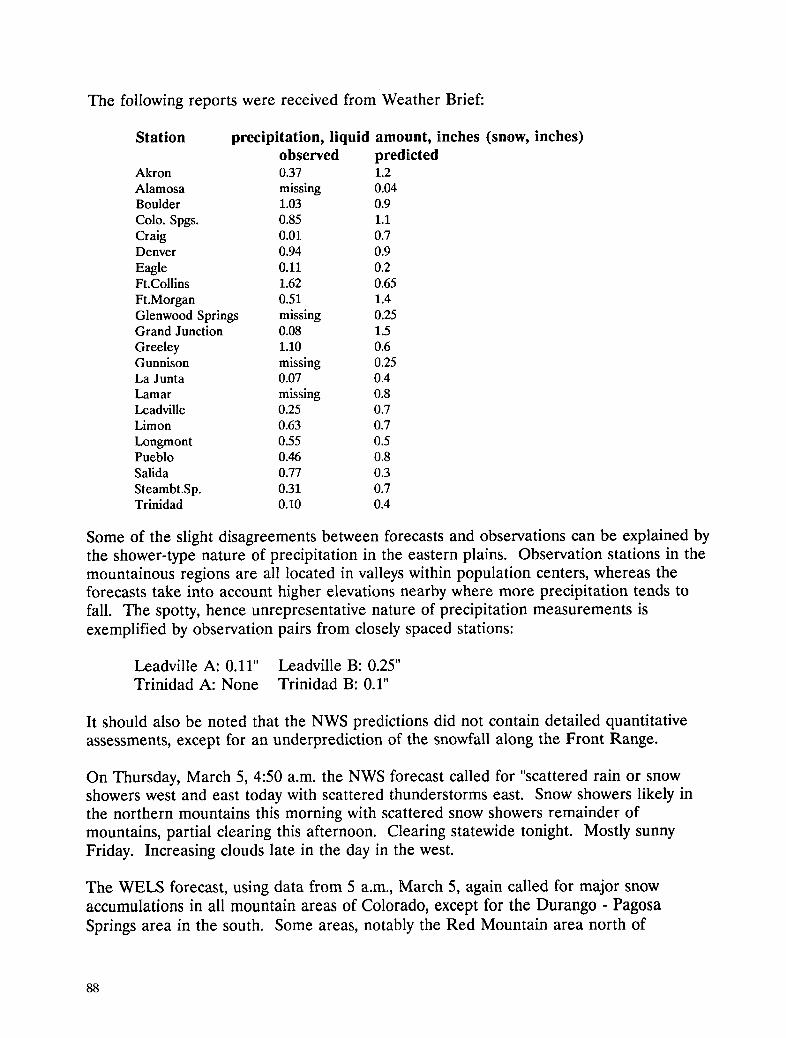
The following reports were received from Weather Brief:

Station precipitation, liquid amount, inches (snow, inches)observed predicted

Akron 0.37 L2

Alamosa missing 0.04Boulder 1.03 0.9

Colo. Spgs. 0.85 1.1Craig 0.01 0.7Denver 0.94 0.9

Eagle 0.11 0.2Ft.Collins 1.62 0.65

Ft.Morgan 0.51 1.4Glenwood Springs missing 0.25Grand Junction 0.08 1.5

Greeley 1.10 0.6Gunnison missing 0.25La Junta 0.07 0.4

Lamar missing 0.8Leadville 0.25 0.7Limon 0.63 0.7

Longmont 0.55 0.5Pueblo 0.46 0.8Salida 0.77 0.3

Steambt.Sp. 0.31 0.7Trinidad 0.10 0.4

Some of the slight disagreements between forecasts and observations can be explained bythe shower-type nature of precipitation in the eastern plains. Observation stations in themountainous regions are all located in valleys within population centers, whereas theforecasts take into account higher elevations nearby where more precipitation tends tofall. The spotty, hence unrepresentative nature of precipitation measurements isexemplified by observation pairs from closely spaced stations:

Leadville A: 0.11" Leadville B: 0.25"Trinidad A: None Trinidad B: 0.1"

It should also be noted that the NWS predictions did not contain detailed quantitativeassessments, except for an underprediction of the snowfall along the Front Range.

On Thursday, March 5, 4:50 a.m. the NWS forecast called for "scattered rain or snowshowers west and east today with scattered thunderstorms east. Snow showers likely inthe northern mountains this morning with scattered snow showers remainder ofmountains, partial clearing this afternoon. Clearing statewide tonight. Mostly sunnyFriday. Increasing clouds late in the day in the west.

The WELS forecast, using data from 5 a.m., March 5, again called for major snowaccumulations in all mountain areas of Colorado, except for the Durango - PagosaSprings area in the south. Some areas, notably the Red Mountain area north of

88

Durango, could expect up to 40 mm (liquid) precipitation or 16" of new snow. That areahad witnessed avalanches which cost the life of one highway maintenance person.

Station precipitation, liquid amount,inches (snow, inches)observed predicted

Akron 0 none, trace possibleAlamosa Trace none, but precip within 20 milesBoulder none none

Colo. Spgs. none 0.3Craig 0.08 0.8

Denver 0.08 none, but precip 20 mi to southEagle Trace TraceFt.Collins 0.01 none to Trace

Ft.Morgan 0.01 none to TraceGlenwood Springs missing 0.05Grand Junction 0.3 0.8

Greeley 0.02 noneGunnison none 0.8

La Junta 0.03 none, showers in areaLamar missing none, showers in areaLeadville missing 0.6Limon Trace 0.04

Longmont none nonePueblo 0.03 Trace

Salida missing 0.2Trinidad none none

The WELS forecast from 5 a.m. data, March 6, confirmed the clearing trend predictedby NWS, with the potential of just a few showers lingering on over the State.

NWS issued a winter storm watch effective the evening of Saturday, March 7, to Sunday,March 8, for the central and southern mountains, the Four Corners and the San LuisValley.

The WELS forecast for this period indicated only widely scattered, isolated lightprecipitation activity in the State. Weather Brief confirms a few scattered showers.

4.4.23. March 8 - 9, 1992, the "Blizzard of 1992"

The NWS forecast issued at 6:30 a.m. MDT, Sunday March 8, and received throughWeather Brief stated: "The winter storm will continue to develop today and should bringprecipitation to all of Colorado by this afternoon. A heavy snow warning has beenissued for some of the mountain areas of Colorado today and tonight, and snowadvisories have been issued for much of the rest of the State." At 5:30 a.m. some detailswere given as follows: "Periods of snow today mountains and west. Accumulations of 6to 12 inches San Juan and central mountains south of Aspen today, 3 to 6 inches possiblelower elevations of southwest. Increasing clouds with scattered showers and a fewthunderstorms east. Turning windy and colder afternoon with rain changing to snow.

89

Periods of snow tonight mountains and east, decreasing west. Scattered snow showersMonday mountains and east, decreasing late. Partly cloudy west."

The news media predicted anywhere from 1 to 8" for this storm before it hit, focussingon the Denver area. While the storm was in progress, advisories were upgraded to snowfrom 8 to 16 inches, which still underestimated the strength of this blizzard, the worst inseveral years. The media dubbed it "the Blizzard of 1992."

The WELS forecast started with 5 a.m. data of Sunday, March 8. By 11 a.m. strongwinds from the northeast were expected over the northeastern plains, with temperaturesnear freezing at 600 m above terrain (in the lower 40s near the ground) in theDenver/Boulder area (Fig. 4.29). Precipitation was expected by this time mainly in themountains to the west and north of Boulder (Fig. 4.30), in strong contrast to the NWSprediction which expected the storm to hit the southwestern parts of the State.Convective (shower and thunderstorm-type) precipitation was predicted by 11 a.m. forthe region between Denver and Colorado Springs, and also over the northeastern plains(Fig. 4.31). The P.I. recalls threatening skies to the west and south of Boulder, startingaround 10 a.m., with ceilings dropping below the peaks of the Flatiron Mountains. Astrong thunderstorm hit Boulder a little after 2 p.m. Thus, the WELS forecast was"premature" by a few hours, but from thereon beautifully matched the sequence ofevents. By 5 p.m. 30 mm more liquid water (ca. 1 ft of snow) were expected in themountains west of Boulder, and heavy rain turning into snow is indicated to thesoutheast of Ft. Morgan (Fig.4.32). Although predicted temperatures remained nearfreezing in the northeastern plains, the heavy snow itself produced enough cooling (notaccounted for in the prediction model) to make it stick to the ground. By Mondaymorning WELS forecast more than 100 mm (40" of snow) in the foothills and mountainswest of Boulder. Near 90 mm (ca. 2 ft of snow, taking into account early rain and highmoisture content) were expected in the region between Ft. Morgan and Limon (Fig.4.33).

The P.I.'s notes indicate that in Boulder (eastern suburb) intermittent heavy showers,some with hail 1/4 to 1/2" in diameter, turned into snow by about 6 p.m. By 10 p.m.snow accumulation amounted to about 9" on driveways, more on grass. Winds were

gusty with a northerly component. There were numerous, short power outages. Treessuffered heavily under the burden of wet snow. By 8 a.m. on Monday, March 9, 21" weremeasured on driveways east of Boulder. The snow was heavy, wet, and melting near thebottom, but light and dry in the upper 2/3. Mr. Steven Carlson (CDOT Greeley)confirmed heavy blizzard conditions. He mentioned that several snow plows got lost inthe blizzard and were stuck out on the roads mainly south of Ft. Morgan. Many roadclosures were in effect. Highway 36 between Denver and Boulder iced over in theevening of the 8th and turned into a gigantic parking lot for hundreds of abandoned cars.Many businesses in Boulder were shut down Monday, and even on Tuesday. On Mondayunplowed streets could be negotiated only in four-wheel drive vehicles. Fortunately,snow removal was aided by rapidly clearing weather in the afternoon of Monday, and bywarm weather following the blizzard. Unfortunately, heavy snow accumulation on thesatellite antenna prevented data reception on Monday morning. Therefore WELS couldnot follow the aftermath of the storm with a prediction.

90

The difficulties of verifying the storm effects become apparent from the inconsistenciesbetween observations: Ft. Collins, for instance, reported 1.18" of liquid water turninginto 13" of snow, whereas Boulder received 20" of snow out of 0.74" of liquid water (froma report not contained in Weather Brief). According to Fig. 4.33, Ft. Collins lies on aline indicating 30 mm (1.2") of liquid-equivalent precipitation, while Boulder and Denverpredictions were in excess of 40 mm (1.6") which would be more in line with 20" of snow.However, the Denver observer only reported 11" of snow (0.67" liquid). Wheat Ridge onthe west side of Denver reported 1.86" of liquid (15" of snow). In good agreement, ourforecast would place this latter location at somewhat less than 50 mm (ca. 1.9") of liquidprecipitation.

There is no doubt that the "southern" storm predicted by NWS did not materialize:Alamosa in the San Luis Valley went from a 6" snow cover on the day before the allegedstorm to a 4" cover after the storm. Trinidad reported only a trace of precipitation. TheWeather Brief report, unfortunately, shows lots of "missing" data.

Station precipitation, liquid amount, inches (snow, inches)observed predicted

Akron 0.60 2.0

Alamosa missing noneBoulder missing 1.8Colo. Spgs. 1.07 1.6Craig 0.06 0.8Denver 0.67 1.8

Eagle 0.12 0.1Ft.Collins 1.18 1.2

Ft.Morgan missing 1.2Glenwood Springs missing TraceGrand Junction 0.08 0.08

Greeley missing 0.8Gunnison missing 0.1La Junta 0.14 none, showers in area

Lamar missing none, showers in areaLeadville missing 0.8Limon 0.32 0.4

Longmont missing 1.2Pueblo 0.02 none, precip 10 miles to westSalida missing 0.1Trinidad Trace none

4. 4.24. March 17 - 20, 1992

The WELS forecast starting with 5 a.m., March 17, anticipated precipitation in themountains north of Durango and between Grand Junction and Gunnison between 5 p.m.and 5 a.m. Accumulations of up to 20 mm (0.8") liquid-equivalent were expected. GrandJunction, at the very edge of the predicted precipitation area, reported a trace.

At 6:30 a.m. NWS (Weather Brief) predicted "scattered rain and snow showers will beover the west and southeast today and tonight with rain and snow likely from the Palmer

91

Divide region (south of Denver) into the northeast. Periods of snow will continue overthe mountains with 2 to 5 inches of new snow possible over the northern and centralmountains...."

The WELS forecast agrees with this rather generic prediction, and provides additionaldetail.

NWS and WELS forecasts for March 19/20 also are in general agreement. Lightprecipitation is anticipated over the mountains.

4.4.25. March 24 - 25, 1992

At 6:30 p.m. on the 23rd NWS (Weather Brief) issued the following prediction: "A fastmoving storm in southern California early this morning will move to the Four Corners bysunset today. As of 5 a.m. light rain showers had already started at Grand Junction."(Note: This rain was predicted by WELS, and was expected to extend into the mesa tothe east as snow.) At 3:55 a.m. on the 24th NWS downgraded this forecast to: "Partlycloudy statewide with widely scattered showers and thunderstorms this afternoon in theeast and snow showers likely in the northern mountains. The WELS forecast, issuedwith 5 a.m. data on the 24th, agreed very well with this "generic" forecast, but providedadditional details, especially over the mountains.

92

5Outlook

Roadweather Pro is now proven and ready for deployment throughout the State ofColorado, and to be customized for deployment and operational use by the other snowstates.

(1). State of Colorado. CDOT has requested that WELS prepare a proposal toimplement Roadweather Pro statewide. As a result of the SHRP-IDEA contract, andthe concurrent contract with CDOT, WELS Weather Central is in place, and digitizedterrain and road networks for the state are in place. To fully deploy Roadweather Pro,the following requirements will have to be satisfied:

• Man and operate WWC on a 24 hours a day, seven days a week schedule.

• Upgrade PIWPS, and the GUI to accommodate all maintenance sections andsenior highway maintenance supervisors.

• Establish a communications switch at WWC to distribute the periodic forecasts(data) to the users, and handle the volume of customer service calls (voice anddata) anticipated.

• Deploy the appropriate computers and modems to the users (if 386/20 typecomputers with 9600 Baud modems are already on-site, WELS or the state canconfigure the computers to share current applications with Roadweather Pro'sGUI).

• Contract with the state run WAN (Wide Area Network) for voice and dataconnectivity between WWC and the users.

• Establish a service and maintenance contract with CDOT.

• Establish on-site system training and installation for highway maintenanceoperators.

(2) Other Snow States. Because of WELS experience with the State of Colorado, itanticipates that it could implement Roadweather Pro within three months from the

93

signing of a contract. In addition to those issues noted for the State of Colorado, pre-contract negotiations with other snow states will have to include:

• A decision by the state if they desire to contract for WWC services, or opt for a"turnkey" system which includes data reception, decoding, analysis and numericalprediction. In most highway maintenance scenarios contracting for services willbe much less expensive than running a meteorological shift operation 24 hours aday and 7 days a week, and making a new capital investment in computer andcommunications hardware and software.

• Identify the source of a state approved GIS. If the state already owns a GIS,WELS can include access to it as no-cost GFE. As with the State of Colorado,

WELS will have to prepare topographic and road networks for each region of thestate as an important customization step.

• Included in system development and deployment must be time to test newlocations, using historical situations, to insure that each system component worksproperly, especially with the linkage to new terrain backgrounds.

• And as with the State of Colorado, access to state-run and -operated voice anddata communications networks will have to be resolved to establishcommunications between WWC and the state users.

94

Appendix A

Roadweather Pro

95

Roadweather Pro (Release 1.01) (Beta Test Version)

1. System Requirements

Computer based on Intel 386 or 486 chip, with at least 10MB hard disk space available.

VGA monitor

MS-DOS 3.0 or higherMicrosoft mouse installed with appropriate driver

The system may run with other configurations as well, but has not yet been tested out.

Note: This is a Beta Release that still may contain "bugs". If any are found, pleasecontact us with a description of reproducible procedures that caused the undesiredperformance. We appreciate your help and cooperation.

2. Program Installation

Place the "INSTALL" diskette in Drive B.

When in the root directory of Drive C, at the DOS prompt C: > type

b:install then hit <ENTER>.

The program will automatically generate directories C:\WELS\EXEC andC:\WELS\DATA needed for program execution and data manipulation. If suchdirectories already exist, they will not be affected by the installation procedure. Thenseveral executable files are automatically transferred to the directory C:\WELS\EXEC,and an experimental data file (FILE.DAT) is copied to the directory C:\WELS\DATA.

The installation procedure automatically executes the file ROADPRO.EXE which nowresides in the directory C:\WELS\EXEC, allowing you to manipulate the experimentaldata file. If you wish to run the Roadweather Pro program again after having exited it,move to the directory C:\WELS\EXEC. (While in the root directory C: >, type CD\WELS\EXEC.) Then type ROADPRO < ENTER> to execute the program.

97

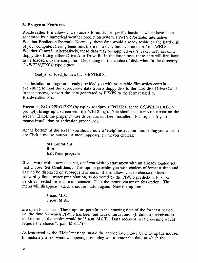
3. Program Features

Roadweather Pro allows you to access forecasts for specific locations which have beengenerated by a numerical weather prediction system, PIWPS (Portable, InteractiveWeather Prediction System). Normally, these data would already reside on the hard diskof your computer, having been sent there on a daily basis via modem from WELSWeather Central. Alternatively, these data may be supplied via "sneaker net", i.e. on afloppy disk fitting either Drive A or Drive B. In the latter case, these data will first haveto be loaded into the computer. Depending on the choice of disk, when in the directoryC:\WELS\EXEC type either

load a or load b, then hit < ENTER >.m

The installation program already provided you with executable files which containeverything to load the appropriate data from a floppy disk to the hard disk Drive C and,in that process, convert the data generated by PIWPS to the format used byRoadweather Pro.

Executing ROADPRO.EXE (by typing roadpro <ENTER> at the C:\WELS\EXEC>prompt), brings up a screen with the WELS logo. You should see a mouse cursor on thescreen. If not, the proper mouse driver has not been installed. Please, check yourmouse installation or activation procedures.

At the bottom of the screen you should note a "Help" instruction line, telling you what todo: Click a mouse button. A menu appears, giving you choices:

Set ConditionsRun

Exit from program

If you work with a new data set, or if you wish to start anew with an already loaded set,first choose "Set Conditions". This option provides you with choices of forecast time anddate to be displayed on subsequent screens. It also allows you to choose options inconverting liquid water precipitation, as delivered by the PIWPS prediction, to snowdepth as needed for road maintenance. Click the mouse cursor on this option. Themenu will disappear. Click a mouse button again. Now the options

5 a.m.M.S.T

5 p.m.M.S.T

are open for choice. These options pertain to the starting time of the forecast period,i.e. the time for which PIWPS has been fed with observations. (If data are received inmid-morning, the choice would be "5 a.m.M.S.T." Data received in late evening wouldrequire the choice "5 p.m.M.S.T.")

As instructed by the "Help" message, make the appropriate choice by clicking the mouse.Immediately a text window appears, prompting you to enter the date at which the

98

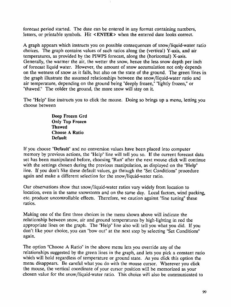
forecast period started. The date can be entered in any format containing numbers,letters, or printable symbols. Hit < ENTER > when the entered date looks correct.

A graph appears which instructs you on possible consequences of snow/liquid-water ratiochoices. The graph contains values of such ratios along the (vertical) Y-axis, and airtemperatures, as provided by the PIWPS forecast, along the (horizontal) X-axis.Generally, the warmer the air, the wetter the snow, hence the less snow depth per inchof forecast liquid water. However, the amount of snow accumulation not only dependson the wetness of snow as it falls, but also on the state of the ground. The green lines inthe graph illustrate the assumed relationships between the snow/liquid-water ratio andair temperature, depending on the ground being "deeply frozen, .... lightly frozen," or"thawed." The colder the ground, the more snow will stay on it.

The "Help" line instructs you to click the mouse. Doing so brings up a menu, letting youchoose between

Deep Frozen GrdOnly Top FrozenThawedChoose A RatioDefault

If you choose "Default" and no conversion values have been placed into computermemory by previous actions, the "Help" line will tell you so. If the current forecast dataset has been manipulated before, choosing "Run" after the next mouse click will continuewith the settings chosen during the previous manipulation, as displayed on the "Help"line. If you don't like these default values, go through the "Set Conditions" procedureagain and make a different selection for the snow/liquid-water ratio.

Our observations show that snow/liquid-water ratios vary widely from location tolocation, even in the same snowstorm and on the same day. Local factors, wind packing,etc. produce uncontrollable effects. Therefore, we caution against "fine tuning" theseratios.

Making one of the first three choices in the menu shown above will indicate therelationship between snow, air and ground temperatures by high-lighting in red theappropriate lines on the graph. The "Help" line also will tell you what you did. If youdon't like your choice, you can "bow out" at the next step by selecting "Set Conditions"again.

The option "Choose A Ratio" in the above menu lets you override any of therelationships suggested by the green lines in the graph, and lets you pick a constant ratiowhich will hold regardless of .temperature or ground state. As you click this option themenu disappears. Be careful what you do with the mouse cursor. Wherever you clickthe mouse, the vertical coordinate of your cursor position will be memorized as yourchosen value for the snow/liquid-water ratio. This choice will also be communicated to

99

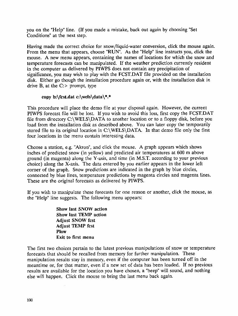
you on the "Help" line. (If you made a mistake, back out again by choosing "SetConditions" at the next step.

Having made the correct choice for snow/liquid-water conversion, click the mouse again.From the menu that appears, choose "RUN". As the "Help" line instructs you, click themouse. A new menu appears, containing the names of locations for which the snow andtemperature forecasts can be manipulated. If the weather prediction currently residentin the computer as delivered by PIWPS does not contain any precipitation ofsignificance, you may wish to play with the FCST.DAT file provided on the installationdisk. Either go though the installation procedure again or, with the installation disk indrive B, at the C: > prompt, type

copy b:\fcst.dat c:\wels\data\*.*

This procedure will place the demo file at your disposal again. However, the currentPIWPS forecast file will be lost. If you wish to avoid this loss, first copy the FCST.DATfile from directory C:\WELS\DATA to another location or to a floppy disk, before youload from the installation disk as described above. You can later copy the temporarilystored file to its original location in C:\WELS\DATA. In that demo file only the firstfour locations in the menu contain interesting data.

Choose a station, e.g. "Akron", and click the mouse. A graph appears which showsinches of predicted snow (in yellow) and predicted air temperatures at 600 m aboveground (in magenta) along the Y-axis, and time (in M.S.T. according to your previouschoice) along the X-axis. The data entered by you earlier appears in the lower leftcorner of the graph. Snow predictions are indicated in the graph by blue circles,connected by blue lines, temperature predictions by magenta circles and magenta lines.These are the original forecasts as delivered by PIWPS.

If you wish to manipulate these forecasts for one reason or another, click the mouse, asthe "Help" line suggests. The following menu appears:

Show last SNOW actionShow last TEMP action

Adjust SNOW fcstAdjust TEMP fcstPlowExit to first menu

The first two choices pertain to the latest previous manipulations of snow or temperatureforecasts that should be recalled from memory for further manipulation. Thesemanipulation results stay in memory, even if the computer has been turned off in themeantime or, for that matter, even if a new set of data has been loaded. If no previousresults are available for the location you have chosen, a "beep" will sound, and nothingelse will happen. Click the mouse to bring the last menu back again.

100

If there were previous manipulations of forecasts in memory, but you don't want themyou should proceed directly with any of the other menu items. This course of action willsimply overwrite old manipulation files.

Suppose, you want to change the SNOW forecast as delivered by PIWPS. Click on thatmenu item. The menu disappears, and the "Help" line instructs you to click the mouseagain. This time a choice of reasons appears why you might want to adjust the snowforecast:

Timing The timing of the snowstorm is wrong;Import from Other Area The present location may have no snow

predicted, but a neighboring location has amore reasonable forecast showing someprecipitation. The forecast from that locationcan be imported as first guess.

Intensity (much)* The intensity of the snow storm should bechanged by quite a bit;

Intensity (moderate)*

Intensity (little)*Fluke Produces a one-time local adjustmentReturn to Menu

Menu items with asterisk (*) should be clicked on at coordinate positions after theoriginally predicted snowfall began. Noting these exceptions, move the mouse cursor tothe coordinate location marking the time for which a recently received observation holds,and to the snow depth reported. Click the mouse at that cursor location. The newforecast will be displayed on the screen by blue circles and white lines. Clicking themouse will bring back the menu. If no further adjustments are desired, click "Return toMenu". The first menu appears. Choose "Run", and the station which you have justmanipulated (or any other desired station). Clicking "Show last SNOW Action" from themenu recalls the last snow forecast manipulation with green circles and blue lines. Youcan proceed as described above to manipulate this last forecast again. If you are notsatisfied with your old forecast corrections, instead of clicking "Show last SNOW Action"proceed directly to "Adjust SNOW fcst". Any actions taken now will over-write filescontaining the old ones.

If you clicked "Adjust TEMP fcst", another click will bring up reasons why you mightwant to modify the original prediction. The choices offered are:

Timing Moves the predicted temperature curve;Diurnal Var.(Sfc.) Extrapolates from 600m to temperature conditions

near the ground;Max.Temp. Allows you to adjust the predicted maximum

temperature;Min.Temp. Allows adjustment of predicted minimum temperature;

101

Fluke Provides a constant temperature shift (e.g. to allow forurban heat island effects);

Return to Menu

When adjusting for poor timing in the forecast of temperature changes, be sure to clickthe mouse at reasonable choices of values. If the mouse is clicked outside the range oforiginally predicted temperatures, a "beep" will sound and the "Help" message will tellyou that your choice was illegal.

The flexibility granted by this menu should be quite useful. Whereas PIWPS predictsprecipitation reaching the ground, temperature forecasts pertain to a level approximately600 m above terrain. Such temperatures are of meteorological interest, but do notreflect the conditions near the earth's surface. First of all, near 600 m the temperaturevariations between day and night are relatively small. The temperature of the air nearthe ground is strongly affected by sunshine which, in turn, is influenced by cloudiness. Ifyou click the "Diurnal Variation" option, the menu disappears and after another clickyou are given the choices:

Clear

Partly CloudyHigh OvercastLow Overcast.

If precipitation is predicted or observed, it is safe to assume "Low Overcast" conditions.Clicking any of these options provides a reasonable guess for air temperatures near thesurface under the chosen, prevailing conditions.

To allow for road surface conditions which may differ strongly from air temperatures,especially when skies are clear, temperature forecasts should be adjusted again.Observations from sensors embedded in the road pavement, and experience will have toguide the user. It might be expedient to .apply another diurnal variation correction ontop of the one executed before, or to adjust maximum and minimum temperaturesseparately. Clicking on one of the latter choices produces menus with a temperaturescale

+5+4+3+2+1etc.

The appropriate choice is translated into an adjustment of the predicted (and perhapsalready modified) temperature curve.

When you "Run" the Roadweather Pro program again, bring up the "Last TEMP Action".It will be displayed by magenta circles connected by red lines.

102

The "Plow" menu choice still needs to be described. After clicking it, move the mousecursor to a location on the screen which closely describes the time at which the plowspassed the location under consideration. Click the mouse at the appropriate cursorlocation. The snow accumulation expected after plowing will be exhibited by greencircles and green lines. You should use this option only if road surface conditions areyour sole concern. In your next choice "Show last SNOW action" the road state afterplowing will be exhibited.

103

Appendix B

Figures

105

GTS

HSHT RCPT

SYD Raw

DECO

C FU_s/(_.

l +<,,++ co_ j

i r

(Meteorological Charts )

GEO MET

Figure 3.I: Flow diagram of the Basic Meteorological System. For detailedexplanations see text.

107

m

. • oo. G o. °....

t_t_

u _ n 4-

oo

a°°oo°°°a° .. °.° ...°a°.°°°°°l.....°°.°°.°°°°'°t° °°'° a°°°° "° " °

I!

Figure 3.2: Flow diagram describing the full weather and geographic data systems.

108

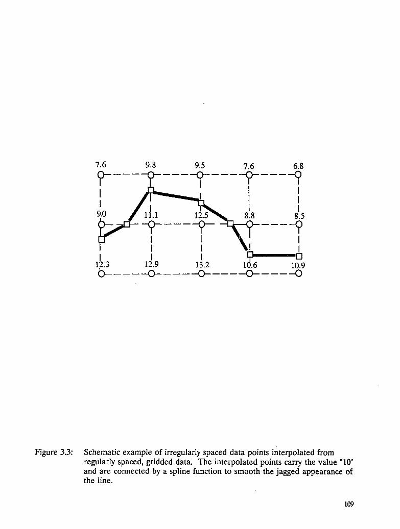
7.6 9.8 9.5 7.6 6.8

_- ? ? 9 ?

1 8.5

?I I I

II I I !_1 []

12.3 12.9 13.2 10.6 10.9b -o o- o o

Figure 3.3: Schematic example of irregularly spaced data points interpolated fromregularly spaced, gridded data. The interpolated points carry the value "10"and are connected by a spline function to smooth the jagged appearance ofthe line.

109

• / I-I ./ ........

..... x'_ / I.i.s ........

" -_" -'p._--,-" . . I .., _• • _'_ _/'J_ • • "_ _. "l .........

• ....,'--. ........i I "a

o o

• ,_':-_T'v"_.....'.-.'_ : ,_. ._. .I ..... >_.:,,-.-'-.-. . . .

• n _ . -J

_. "'::._..... ,: ...... -............ t "t-" t.... t" " "= "l "_ .......

_.-- -" t .t I

l -- _ l tI .......

• " " " " "14 . . • ,i • " "1 -s r-_ ......• • • |_,_, .....r

i" " " t" " " t "l-'s'-_l" "_ .... l" " _ .....

I

.-'l I I /.... | • • • • • • • _o i i

r- -- . 4 .I_,_._I

I

" I' I. ,I

• • o .

• • . °

i| • " • ....

I _ ' "1 .......• • o . _ ........

I

. • • _........

I "'-d. " /. " " "

;/L. .. . _ . . . _* • . .I " I I

I _''" I I

I" * "_". .. ! ......... I .........

Figure 3.4 Domain over which the PIWPS model is run in its present configuration.Dots indicate grid points of the model. Terrain contours, as the model"sees" them, are drawn for every 200 m.

110

Figure 3.5 Domain of the nested grid model, presently configured for the State ofColorado. Terrain elevations used by the model are drawn at 100 mintervals.

111

Figure 3.6: Conversion of liquid water-equivalent to snow, depending on user's choiceof ground state or of a fix* conversion ratio. Background diagram indicatesembedded conversion algorithms.

112

Figure 3.7: Forecast for snow (blue line), temperatures at 600 m above terrain (redline) and winds ("arrows" with scale indicated near bottom), valid forBoulder, 5 a.m. MST, March 8, 1992, till 5 a.m. March 9. Choose "AdjustSNOW fcst" from menu to arrive at Fig. 3.8.

113

!!:!:!:!:!:!:

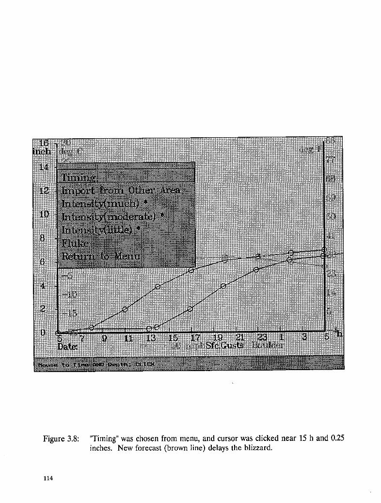
Figure 3.8: "Timing" was chosen from menu, and cursor was clicked near 15 h and 0.25inches. New forecast (brown line) delays the blizzard.

114

Figure 3.9: By choosing "Intensity (much)" from the menu in Fig. 3.8, and clicking thecursor in reference to snow observation at 21 h of >8" a new forecast

(white line) is obtained.

115

Fi 03

Figure 3.10: Clicking the puU-down menu choice "Toggles 3hour precip_ brings up iconboxes which fill up with different colors for predicted rain or snow. Eachsuccessive color step indicates increments of 0.2 inches for rain, and 2inches for snow. The underlying terrain and road network map ofColorado demonstrates the flexibility of the geographic database: Onlyterrain between 4,500 ft and 16,000 ft has been drawn, leaving easternColorado black, thereby showing the Platte and Arkansas River valleys.The "buttons"along the lower edge of the screen have the same functionas the pull-down menus. They also indicate what is currently displayed.The _Play"option provides a time-lapsed display of the forecast times,which can also be clicked on in the menu bar.

116

Help 0_6 09 12_ 15 18_ 21

- 10

•.,4,,-- .20-22 -30

Fig. 3.11: Display of icons symbolizing 3-hour temperature forecast. First appearanceof red in these icons shows temperatures to be above freezing. Clicking onthe "Temperature" button displays a small window with the color code.This window can be moved on the screen. The background shows thetopography and road network for the Boulder/Denver area.

117

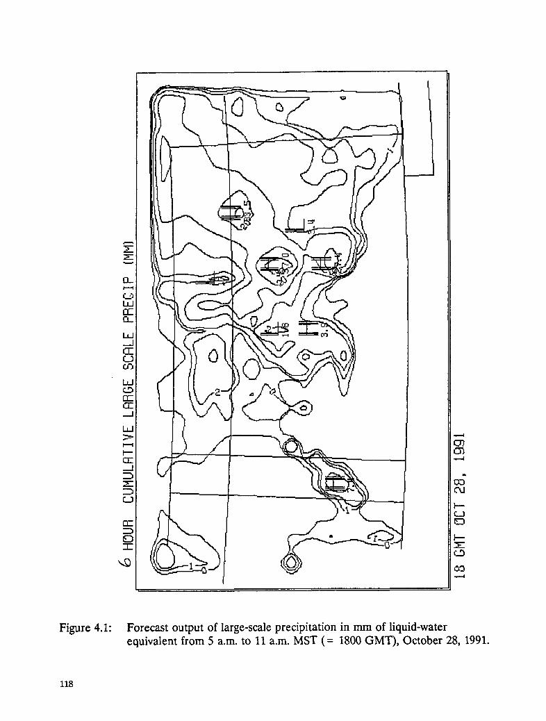
IZ.':x'- ,,, X..

-,,-,-" _-t"a-Li-i ,,..,.

1.1_1

EL.

,,,..._1CCC._I

,,,fr-l--CE __

LJ.__o _

...1

f..3 b-

.,,..-4

Figure 4.1: Forecast output of large-scale precipitation in mm of liquid-waterequivalent from 5 a.m. to 11 a.m. MST (= 1800 GMT), October 28, 1991.

118

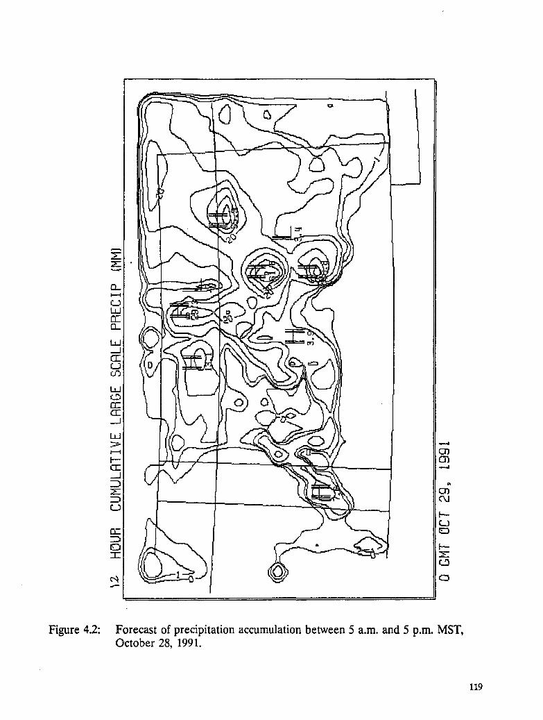
Z It,i,

• v,=..=

,'T'-

_..l (LD

i,mc..,."b

._..I

l,l

l---

J

I---

Figure 4.2: Forecast of precipitation accumulation between 5 a.m. and 5 p.m. MST,October 28, 1991.

119

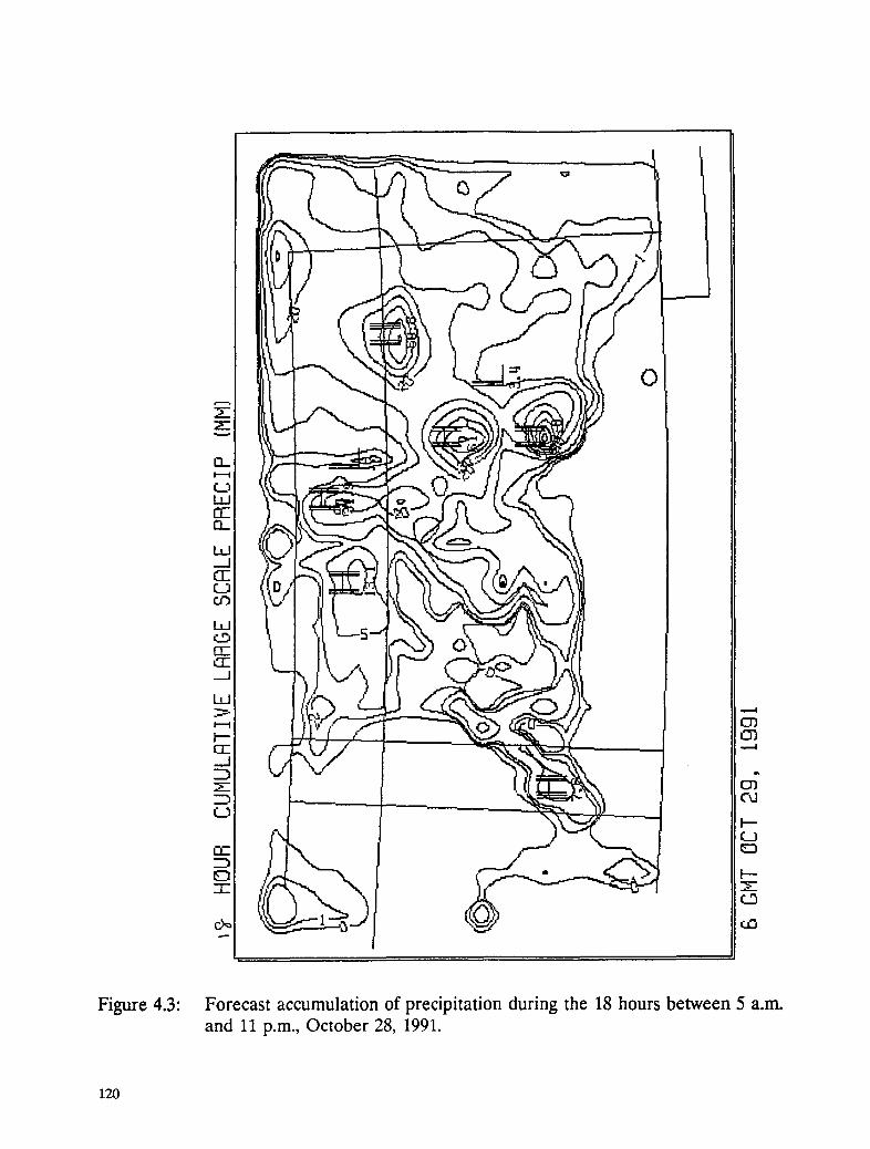
Figure 4.3: Forecast accumulation of precipitation during the 18 hours between 5 a.m.and 11 p.m., October 28, 1991.

120

+C

_,| .I.s "_lr.)1;l, 't

L ._F

+n4 6

,_L.t D

+C (.K

+H ._.s4 p

-I.L .(.L

4}I

tO "tP 4"1 l

k18 HOURHINDF]EI_D IS[GHR61 (H/S)

..... . .it 0 1 po#,t, el tl ¢/_ ,..o,..,,_...

,..,._4.,t._',.ll//,lT_,..tl,t .... _, ,_

...... ,, , , , _ s r ! _ | / 2... , ,, ........ , , , ,

•_ d_toct _g,i_' ' ' ' - - _6.18 HOURTFnPER_TURE tS[r.,nR6_ ICELSIUSl

: ... ,,: • H ,::.,:/tl-- , , _ ,;,

,--'-_.,I ..... I -" -* _'-'.t'. ", L ,". II .-" / fJt' ._ ; III

", ,."'-,.hr-,--J"-" ,_."_ _.,' .,'."/I/:, / / A• ", ',IHH -f. .- I1-, _, ," ,.. ", .-t3.9.," ../.i ",_ _ II

'"_ f

;._"" - o °'. i_

6 GMTOCT2g, tggt

Figure 4.4: Top: City locations by initial letters. Middle: Winds forecast for 11 p.m.MST, October 28, 1991, at 600 m above terrain; top speed (m/sec)indicated by length of arrow and value at lower right of diagram. Bottom:Temperatures forecast for same time at 600 m above terrain in degcentigrade, drawn for every 2 deg; solid lines 0 and positive, dashed linesnegative values (below freezing).

121

J

bm

Figure 4.5: Forecast of precipitation (ram liquid-equivalent) between 6 p.m. and 11p.m. MST, October 29, 1991.

122

Figure 4.6: Forecast of precipitation (mm liquid-equivalent) between 6 p.m. MST,October 29, 1991, and 6 a.m. MST, October 30.

123

Z

IX.I"-"t

I't'l ._.._iE

Figure 4.7: Forecast of precipitation (mm liquid-equivalent) between 6 p.m. MST,October 29, 1991, and 11 a.m. MST, October 30.

124

m +

+

a,

Figure 4.8: Prediction made from 5.a.m. MST data on Nov.14, 1991, for precipitation(ram liquid equivalent) to fall during the 6-hour period between 11 p.m. onthe 14th and 5 a.m. MST on the 15th of November.

125

O

z &

EL_I,-----I

ta..l

EL.

_._1

b-- O

Figure 4.9: Prediction made from 5.p.m. MST data on Nov.14, 1991, for precipitation(mm liquid equivalent) to fall during the 12-hour period between 5 p.m. onthe 14th on the 14th and 5 a.m. MST on the 15th of November.

126

Figure 4.10: Prediction made from 5.p.m. MST data on Nov.14, 1991, for precipitation

(mm liquid equivalent) to fall during the 6-hour period between 11 a.m.

and 5 p.m. MST on the 15th of November.

127

..';r-z

12..

f...)LtAct-t-i

t-"

I----

Figure 4.11: 24-hour precipitation forecast for the period ending at 5 p.m. MST onNovember 15, 1991.

128

_ -+

.4-

Z ,,- -t-

_r-

12..

I,Ior"13-

lid....i

1.1J

t-r--

.....!

ILl

Cj...d

E3re" Z

1£3-r" "_"

¢..9_D

Figure 4.12: Forecast starting with data from 5 a.m. MST on November 27,1991,for the6-hour period ending at 5 p.m. MST on November 28 (00 GMT November

29).

129

Figure 4.13: Forecast for 6-hour period ending at 11 a.m. MST, Novemner 29, 1991.

13o

Figure 4.14: Precipitation forecast starting with data from 5 a.m. MST on December 11,1991, for the 6,hour period ending at 5 p.m. MST on that day.

131

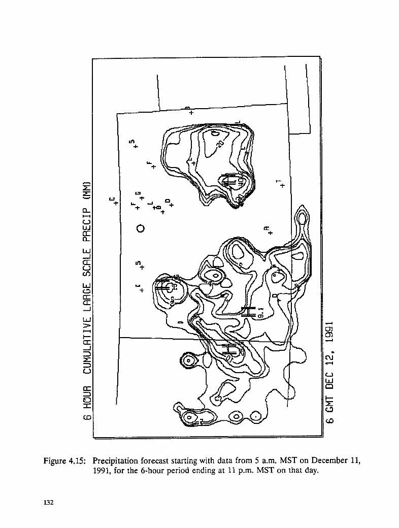
Figure 4.15: Precipitation forecast starting with data from 5 a.m. MST on December 11,

1991, for the 6-hour period ending at 11 p.m. MST on that day.

132

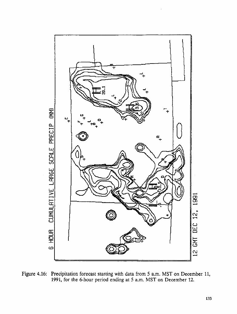
q-

,...4+

Figure 4.16: Precipitation forecast starting with data from 5 a.m. MST on December 11,1991, for the 6-hour period ending at 5 a.m. MST on December 12.

133

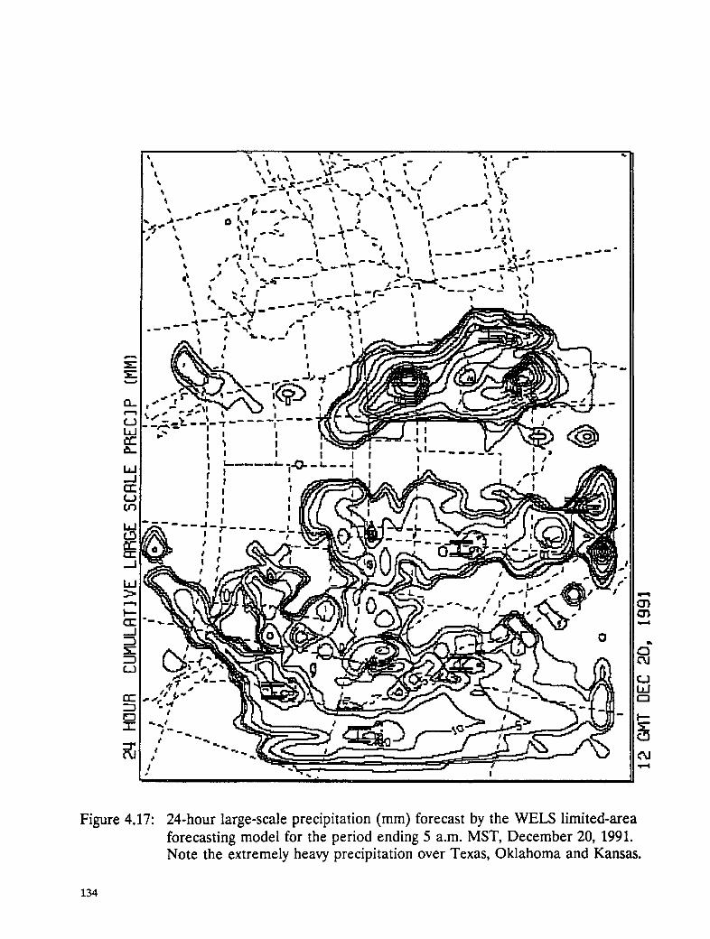
I:,,i¢" % I. "i _ l _ _ ..'_. : .% ",l l- - I _ _ J _ ..... _ p _ I j - _ -

G_ " _ ",_-- .... " _"'_--'-.-,L'------ " _ I

t '% % t _ -- -- --17"'. _, %,-" I : l I,, ?..,,,,..._-- ,, '- _.,,. ,

_=t---- j _ " -- I

o_ • -- _" ,." -- ' I _ . _J"J' __ "./'J"t4'1

.'--:I--,_.-__---,-_ .... i t_!,k _ ( ', i _F_-.b_

_"_ i _ i i _ .... : : If" _, , , i i ::, -I . .,._ -- I i I sI _'-- .... _ I,. 4 l-- i - -- i oo...=j f I I l

I l I "T"l l l l

('-) I ! oOr) I _ IILid ----I IC.D ,-r ...... ,-I e¢'r"C_ _ i._I t

l,l

"" 0"_I"-CI:: ",-'--I

d"'1 ff_l

_J

.-r-

Figure 4.17: 24-hour large-scale precipitation (mm) forecast by the WELS limited-areaforecasting model for the period ending 5 a.m. MST, December 20, 1991.Note the extremely heavy precipitation over Texas, Oklahoma and Kansas.

134

,1 _ ';x

,., .I.'' I%,I _ ..---_ I ,, , S It,,.,," l ',",

_- _ _I I / I _---- # __

l, S _ _ _ _ _.-" ', N,_.___ _ _ ---- ,, ,, .

', "._ _. t .. -- --17". ', .-" I . _'_.-,]----,,_ - _ II

- ___ UFlllllI

,-' _--J_-+ _ .--.J#'r'_ __'_I_'7._._ ((<_II

:":!!!.iI I I /

, , ,, _':/,_//_\ ,_11

; : ., ; : o; 3_<._V_III,_, ' _ ,,--_ _- ' ,I _ F ; --"_-----_'-_l_#TJII

7-"--- : ; ; ." '_ ' -.'"___ _{_ I --_.r r ,, -" _ (:3

"_e t _ -_--.-.. " ..,2"- ,-- .... r-',"_ _-- l ---___ _ _ - I--

i i

Figure 4.18: 24-hour convective precipitation (mm) forecast by the WELS model forsame time period as in Fig. 4.17. The amounts shown in this figure have tobe added to those in Fig. 4.17 to yield total 24-hour precipitation.

135

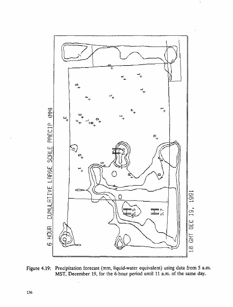
1 /'-"- /I ",Ik',----"-'-_.____J" l I /" ".. ', ' !,

m,4-

,..I

t_1

u. "t"

Figure 4.19: Precipitation forecast (mm, liquid-water equivalent) using data from 5 a.m.MST, December 19, for the 6-hour period until 11 a.m. of the same day.

136

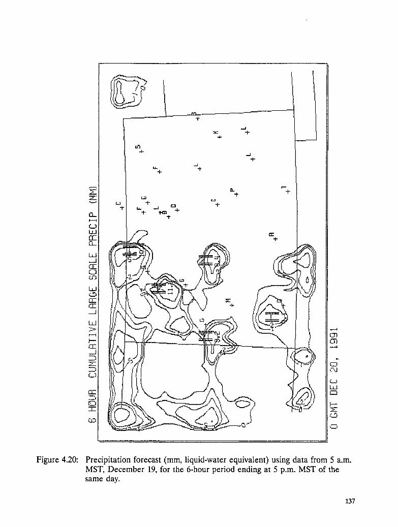
m t

..J

.4-

-4-

.t-...I

Figure 4.20: Precipitation forecast (mm, liquid-water equivalent) using data from 5 a.m.MST, December 19, for the 6-hour period ending at 5 p.m. MST of thesame day.

137

4- _j.t-

,.d

u. "1"Z a. +

"" _ +u. __D t:a -I-"i- _12..

1I--'1

¢..)ILl a:rt"o_

t.13_.J02 tn

t.t_l

_r- ,.,.jr OOd

ILl

ED _---r-

¢..9¢.O =

¢.O

, m

Figure 4.21: Precipitation forecast (mm, liquid-water equivalent) using data from 5 a.m.MST, December 19, for the 6-hour period ending at 11 p.m. MST of thesame day.

138

,.Ioe"t"

Figure 4.22: Precipitation forecast (mm, liquid-water equivalent) using data from 5 a.m.MST, December 19, for the 6-hour period ending at 5 a.m. MST onDecember 20.

139

-t-

....I,..- q.

tt_..I

+-.I

o_ "t""t-

Figure 4.23: Precipitation forecast (mm, liquid-water equivalent) using data from 5 a.m.

MST, December 20, for the 6-hour period ending at 11 a.m. MST on the

same day.

140

...I

4-

Figure 4.24: Precipitation forecast (mm, liquid equivalent), starting at 5 a.m. MST,January 7, 1992, for the 6-hour period ending at 11 a.m. MST on the sameday.

141

k +

...I

_- -F,4,,

.1-

Z a. +.t-

_Q.. "_"t"

I"---i

Lul _-_--,,, G

....I(I2r__.l L

w

n'-

_...1

f-J ---7CIZ

O b---r- _

ii

Figure 4.25: Precipitation forecast (ram, liquid equivalent), starting at 5 a.m. MST,January 7, 1992, for the 6-hour period ending at 5 p.m. MST on the sameday.

142

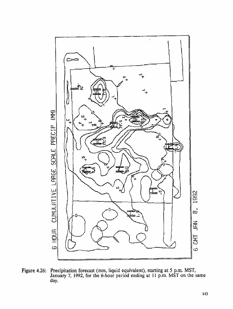
Figure 4.26: Precipitation forecast (mm, liquid equivalent), starting at 5 p.m. MST,January 7, 1992, for the 6-hour period ending at 11 p.m. MST on the sameday.

143

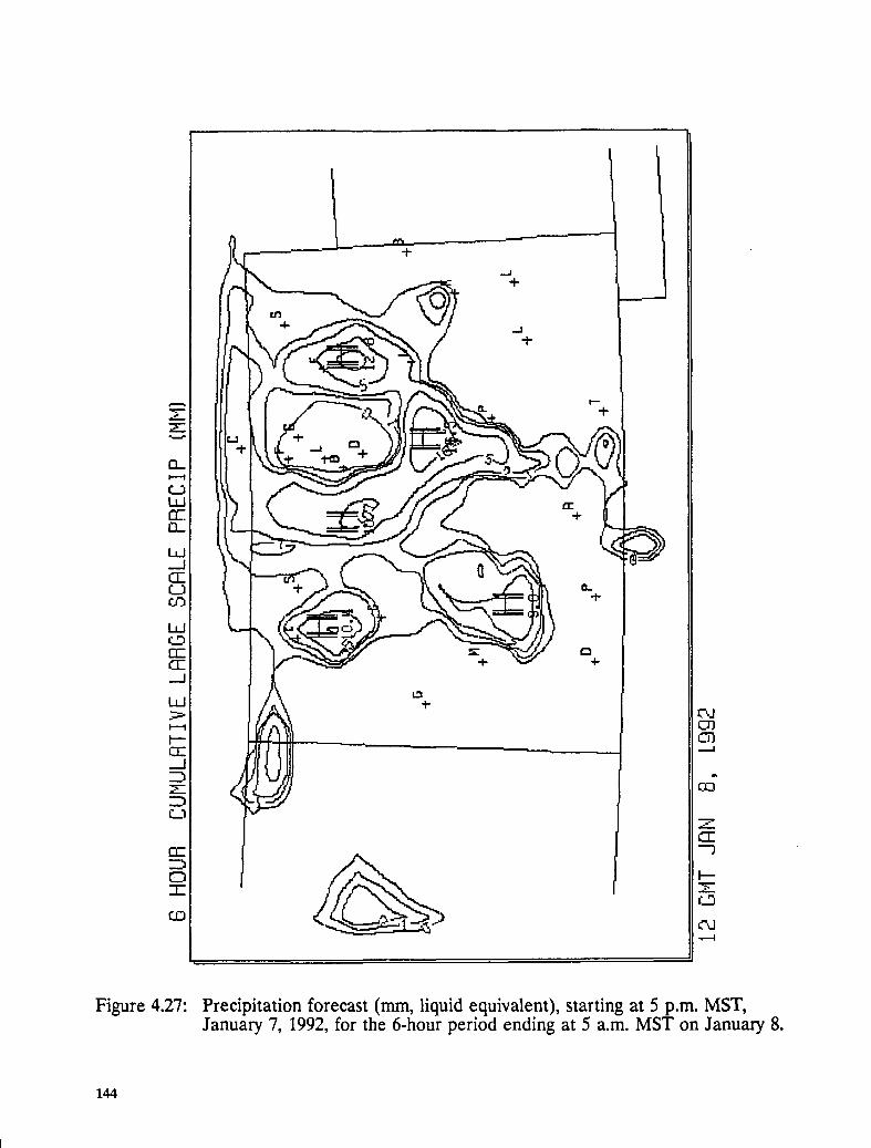
Figure 4.27: Precipitation forecast (mm, liquid equivalent), starting at 5 p.m. MST,January 7, 1992, for the 6-hour period ending at 5 a.m. MST on January 8.

144

tL

.d

Or

Figure 4.28: Precipitation forecast (mm, liquid equivalent), starting at 5 p.m. MST,Janua_ 7, 1992, for the 6-hour period ending at 11 a.m. MST on January8.

145

Figure 4.29: Forecast starting at 5 a.m. MST, March 8, 1992, for 11 a.m. MST on sameday, of temperatures (deg centigrade drawn at 2-deg intervals, 600 m aboveterrain) and winds (m/sec, 600 m above terrain). Solid lines aretemperatures 0 deg or higher, dashed lines are temperatures belowfreezing. Scale for longest wind arrows is given in lower right of diagram.

146

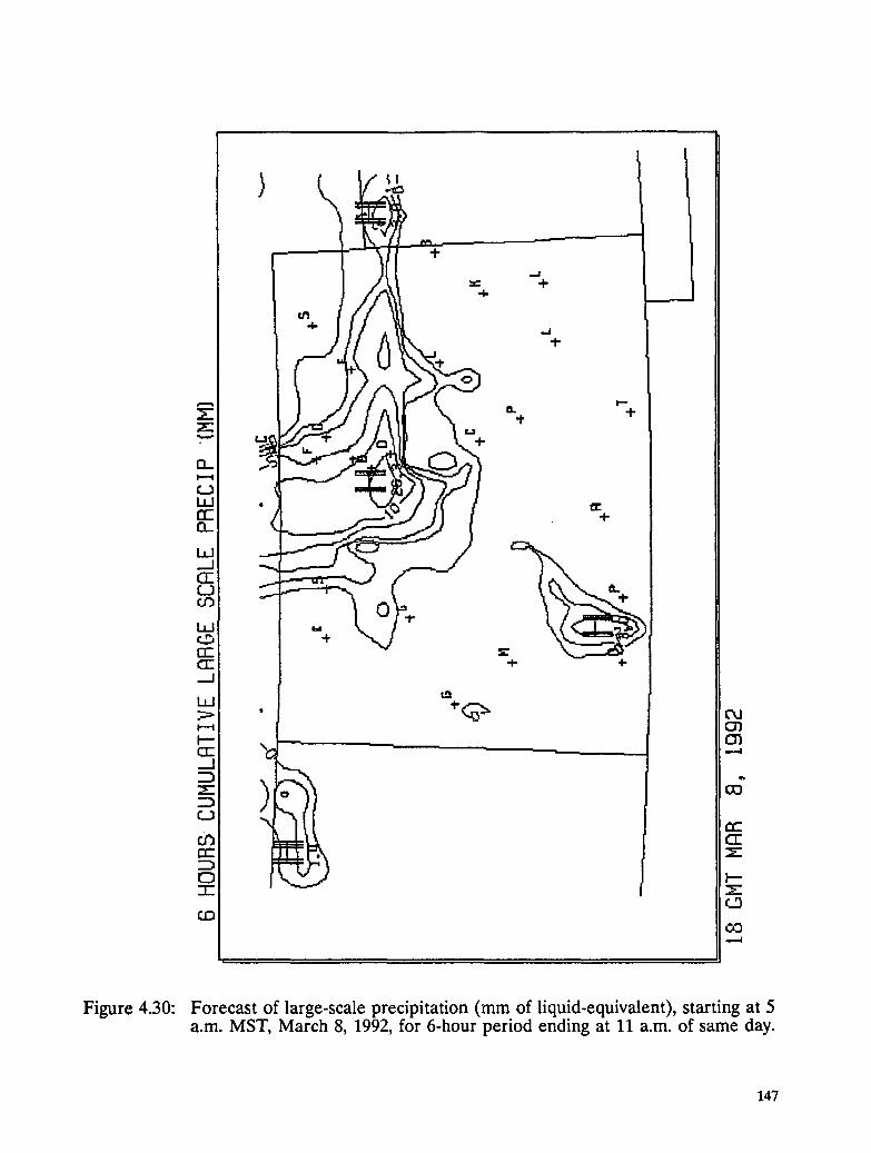
-l-

..dne -I-

.4-

,.J.p

Figure 4.30: Forecast of large-scale precipitation (mm of liquid-equivalent), starting at 5a.m. MST, March 8, 1992, for 6-hour period ending at 11 a.m. of same day.

147

t.d_=. t'M

-..I

z a5

t...._ e¢"

O-r" _'y-x"

• ¢..3

c.O ¢O.,....4

Figure 4.31: Forecast for convective (small-scale) precipitation (mm of liquid-equivalent) for same time period as in Fig. 4.30.

148

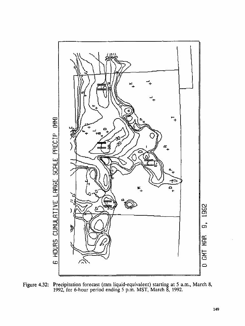
,,.,d"" 4-

,4-

..I

Figure 4.32: Precipitation forecast (mm liquid-equivalent) starting at 5 a.m., March 8,1992, for 6-hour period ending 5 p.m. MST, March 8, 1992.

149

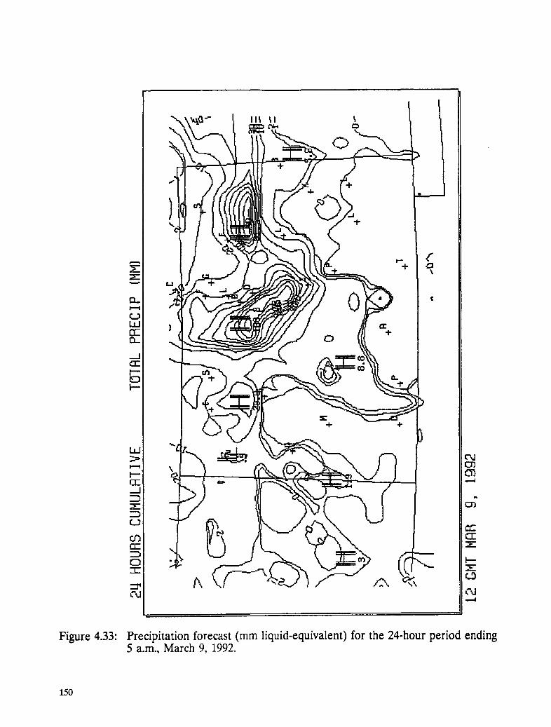
rr 0 !I--"

19I--

-I- 4-

Figure 4.33: Precipitation forecast (mm liquid-equivalent) for the 24-hour period ending5 a.m., March 9, 1992.

150

For additional information, please call or write:WELS Research Corporation

5114 Balcones Woods Drive #307, Suite 299Austin, Texas 78759

512/346-4059fax: 512/345-3743