integration of a coordinating system with …integration of a coordinating system with conventional...
TRANSCRIPT
INTEGRATION OF A COORDINATING SYSTEM WITH CONVENTIONAL METROLOGY
IN THE SETTING OUT OF MAGNETIC LENSES OF A
NUCLEAR ACCELERATOR
FRED J. WILKINS
November 1989
TECHNICAL REPORT NO. 146

PREFACE
In order to make our extensive series of technical reports more readily available, we have scanned the old master copies and produced electronic versions in Portable Document Format. The quality of the images varies depending on the quality of the originals. The images have not been converted to searchable text.

INTEGRATION OF A COORDINATING SYSTEM WITH CONVENTIONAL
METROLOGY IN THE SETTING OUT OF MAGNETIC LENSES OF A NUCLEAR
ACCELERATOR
Fred J. Wilkins
Department of Surveying Engineering University of New Brunswick
P.O. Box 4400 Fredericton, N.B.
Canada E3B 5A3
November 1989 Latest Reprinting January 1994
© F.J. Wilkins, 1989

PREFACE
This technical report is a reproduction of a thesis submitted in partial fulfillment of the
requirements for the degree of Master of Science in Engineering in the Department of
Surveying Engineering, September 1989. The research was supervised by Dr. Adam
Chrzanowski, and funding was provided partially by the Natural Sciences and Engineering
Research Council of Canada, the Atomic Energy of Canada Ltd., and by the National
Research Council of Canada's Industrial Research Assistance Program agreement with
Usher Canada Ltd.
As with any copyrighted material, permission to reprint or quote extensively from this
report must be received from the author. The citation to this work should appear as
follows:
Wilkins, F.J. (1989). Integration of a coordinating system with conventional metrology in the setting out of magnetic lenses of a nuclear accelerator. M.Sc.E. thesis, Department of Surveying Engineering Technical Report No. 146, University of New Brunswick, Fredericton, New Brunswick, Canada, 163 pp.

Abstract
Industrial metrology is a discipline of engineering surveys that requires the utmost in
achievable accuracies. The instrumentation used in traditional industrial metrology requires
long painstaking procedures with very skilled craftsmen to obtain the required results. The
introduction of electronic theodolites has changed the approach and the flexibility of
industrial surveys.
The development of coordinating systems, electronic theodolites interfaced to a
microcomputer, provides the capabilities for on line data gathering with simultaneous
processing in all three dimensions. The existing requirements for conventional metrology
of having to access particular lines of sight can be neglected, without loss of accuracy and
with the addition of redundancy, to obtain the coordinate solutions. In addition, groups of
targets can be analysed in virtual real time by determining coefficients for a particular
surface from a least squares fitting. However, the coordinating system and the conventional
techniques each have their own assets, with the integration of the two techniques into a
single system allowing for the full exploitation of each's assets.
A coordinating system, precision three dimensional coordinating system ("P3DCS"),
has been developed at UNB, as a by-product of a project involving the setting out of
components forming a portion of a nuclear accelerator. The algorithms that have been
developed and used for the software development are presented with emphasis placed on
obtaining the optimal accuracies from the system.
The UNB coordinating system was integrated with traditional metrology techniques
in the successful completion of the setting out of Phase II of the Tandem Accelerator
Superconducting Cyclotron ("TASCC") for Atomic Energy of Canada Ltd. ("AECL").
This phase of TASCC involved the precision three dimensional alignment of 67 magnets,
both bending and focussing, to tolerances less than 0.1 mm in the transverse and 0.2 mm
in the along beam line from their nominal locations.
i
Table of Contents
page
Abstract ............................................................................................. i
List of lllustrations ............................................................................... .iv
List of Tables ....................................................................................... vi
Acknowledgements ................................................................................ vii
1. Introduction .................................................................................... 1
2. Electronic Theodolites ........................................................................ 6
2.1 Electronic Circle Measurement.. ................................................ 7 2.1.1 The Wild Dynamic System ............................................. 7 2.1.2 The Kern Static System ................................................ 11
2.2 Electronic and Optical-Mechanical Theodolite Characteristics .............. 15 2.2.1 The Systematic Errors in Theodolite Construction .................. 17 2.2.2 The Random Theodolite Errors ........................................ 22
3. General Overview of Traditional Three Dimensional Positioning ....................... 27
3.1 Three Dimensional Coordinate Systems ....................................... 28 3.2 The Terrestrial Observation Equations ......................................... 34 3.3 Variations Between Local Astronomic Coordinate Systems ................ 38
3. 3.1 Gravimetric Reductions ................................................ 39 3.3.2 Geometric Reductions .................................................. 43
3.4 Design Criteria for Metrology Micronetworks ................................ 48 3.4.1 ScaleDetennination ..................................................... 49 3.4.2 Atmospheric Refraction ................................................ 50 3.4.3 CenteringError .......................................................... 53
4. Algorithms for Coordinating System Software ............................................ 55
4.1 The Theodolite - Computer Interface ........................................... 58 4.1.1 The Communication Protocol.. ........................................ 58 4.1.2 TheDataDecoding ...................................................... 60
4.2 Data Acquisition and Quality Checks .......................................... 62 4.3 Coordinate Determination of the Theodolites in the Project Area ........... 69 4.4 Auxiliary Target Computations and Surface Fitting .......................... 76
5. Positioning Components of the TASCC Linear Accelerator .............................. 84
5.1 Scope of the Project .............................................................. 84 5.2 The Establishing of the Reference Geodetic Micro-Network ............... 89
ii

5. 3 The Setting Out of the Components ............................................ 97 5.3.1 Targetting of the Component Axes .................................... 97 5. 3. 2 The Offset Measurements for the Quadrupoles ...................... 99 5. 3. 3 The Coarse Alignment .................................................. 102 5.3.4 The Fine Alignment ..................................................... 103 5.3.5 The Maintenance of the System ....................................... 108
5.4 The Stability of the Micro-Network ............................................ 110
6. Conclusions and Recommendations ........................................................ 117
References .......................................................................................... 121
Appendix 1 .......................................................................................... 126
Appendix II. ........................................................................................ 136
Appendix 111 ........................................................................................ 140
iii

List of Illustrations
page
Figure 2.1 The Wild Dynamic Measuring System .......................................... 9
Figure 2.2 The Moire Pattern of the Kern Static Measuring System ...................... 12
Figure 2.3 Relationship Between the Three Major Axes of a Theodolite ................. 16
Figure 2.4 Variation of Index Error with Temperature ..................................... 20
Figure 3.1 The Conventional Terrestrial (CT) Coordinate System ........................ 29
Figure 3.2 The Local Astronomic (LA) Coordinate System ............................... 29
Figure 3.3 The Geodetic (G) and Local Geodetic (LG) Coordinate Systems ............ 31
Figure 3.4 The Deflection of the Vertical Components ..................................... 34
Figure 3.5 Maximum Tolerance for Changes in the Deflection of the Vertical .......... 42
Figure 3.6 Rotation About the Z Axis ........................................................ 44
Figure 3.7 Rotation About theY Axis ........................................................ 44
Figure 3.8 Rotation About the X Axis ....................................................... .47
Figure 3.9 Effects of Neglecting the Earth's Curvature ................................... .47
Figure 3.10 Typical Observing Scheme Using the "Free Positioned" Theodolites ....... 52
Figure 4.1 The Primary Software Modules of a Coordinating System ................... 56
Figure 4.2 Flow Diagram for the Theodolite-Computer Interface ......................... 57
Figure 4.3 The Macintosh Plus/SE- Kern E2 Interface .................................... 59
Figure 4.4 Flow Diagram for the Data Acquisition Module ................................ 63
Figure 4.5 Flow Diagram for the Positioning of the Theodolites Module ................ 68
Figure 4.6 Flow Diagram for the Auxiliary Target and Surface Fitting Module ......... 77
Figure 5.1 The TASCC Linear Accelerator .................................................. 86
Figure 5.2 A Schematic Diagram of Phase II ofT ASCC .................................. 87
iv

Figure 5.3 Observation Scheme for Phase IIA Control Survey ........................... 91
Figure 5.4 Observation Scheme for Phase liB Control Survey ........................... 92
Figure 5.5 Datum Defmition for the Control Network ..................................... 94
Figure 5.6 Oblique View of a Quadrupole ................................................... 98
Figure 5.7 The Omnidirectional Conical Target Designed by UNB ...................... 98
Figure 5.8 Theodolite Locations for Quadrupole Offset Determinations ................. 101
Figure 5.9 Typical Theodolite Locations for the Setting Out Survey ..................... 104
Figure 5.10 A Typical Set Up Showing All Instrumentation ................................ 105
Figure 5.11 Section BE-l to BE-3 Aligned with Hardware Installed ...................... 105
v

Table 2.1
Table 5.1
Table 5.2
Table 5.3
Table 5.4
Table 5.5
Table 5.6
Table 5.7
List of Tables
page
Total Expected Error for Theodolites ............................................ 25
Components of Phase ITA ........................................................ 85
Components of Phase liB ........................................................ 85
Statistical Summary of Phase ITA Control Survey ............................. 96
Statistical Summary of Phase ITB Control Survey ............................. 96
Displacements and Error Ellipses (95%) in (x,y) Plane ....................... 112
Displacements and Error Ellipses (95%) in (x,z) Plane ....................... 113
Displacements and Error Ellipses (95%) in (y,z) Plane ....................... 114
Vl

Acknowledgements
There are no research projects that can be concluded without the help and support of
many individuals, whose contributions deserve proper acknowledgement.
Firstly, I would like to thank my supervisor, Dr. Adam Chrzanowski, for providing
the opportunity for me to partake in one of his many research projects and supplying some
of the financial resources available to him from the Natural Science and Engineering
Research Council of Canada. His endless supply of patience and knowledge were drawn
upon many times throughout the research activity as well as in the preparation of this
manuscript. In times of need the opportunities for discussion, encouragement, and
friendship were always available irregardless of his very busy schedule and other
commitments.
Additional financial support for these studies has been obtained from contract
agreements between Atomic Energy of Canada Ltd. with the University of New Brunswick
and Usher Canada Ltd. In particular, I would like to thank Dr. Hermann Schmeing of
AECL for his willingness to disregard his initial reservations, which allowed the
involvement of UNB in the TASCC project.
All surveying projects that involve field work require additional personnel to help
complete the various tasks. In this respect I would like to acknowledge the contributions of
James Secord, Mark Rohde, Peter Stupan, and Pablo Romero for their excellent field work
as well as that from their technical knowledge.
Finally, the most precious acknowledgement of all is that to my wife Adela and our
daughter Danielle. Together they have forfeited countless number of evenings and
weekends to allow me the necessary time to perform the work and complete this
manuscript.
vii

1. Introduction
Industrial metrology is a field of engineering surveys that requires the utmost in
achievable accuracies and almost invariably depends on the results being in real time.
Traditional methods of metrology have involved alignment telescopes, wires (invar,
piano, etc.), calibrated bar sections (for distance), jig transits, autocollimating
instruments, machinists levels (of varying sensitivities and lengths) and other such
instrumentation, which when properly calibrated and used by skilled craftsmen are very
capable of fulfilling the accuracy requirements for most industrial applications.
Positioning of components forming particle accelerators has long been a developing
ground for instrumentation used in industrial metrology and consequently surveying in
general. This is due to the very stringent accuracy requirements of the assemblies,
bordering on or going just beyond the capabilities of the most technologically advanced
instrumentation and methodologies. This in turn, creates very time consuming and
subsequently expensive measurement techniques being performed by very skilled
craftsman.
The European Organization for Nuclear Research ("CERN") has been the most
influential in this expansion of technology throughout their various projects, spanning
back to the construction of the Proton Synchrotron in 1954-59 (Gervaise, 1974) and
covering the Super Proton Synchroton constructed in 1971-76 (Gervaise, 1976). CERN's
prestigious surveying group can be credited with the discovery of the problem involving
the elongation of invar wire with use, first detailed studies of the trilateration method of
positioning stations, and inventing of the "distinvar" (Gervaise, 1976). The findings of
this group have not only been used at other construction sites involving accelerators, but
1

the ramifications of their results can also be seen throughout the various surveying
disciplines.
In recent years the imaginative surveying groups have taken the approach of
developing special accessories to complement existing optical tooling instrumentation. For
example, the surveying group at Los Alamos National Laboratory has constructed special
wedges to install a skewed accelerator beam line (Banke et al., 1985) and a special sine
bar to install deflection mirrors at a particular skewed angle (Banke et al., 1983). The
accessories were required to be able to create an oblique reference plane, which is not
easily accomplished with typical jig transits and alignment telescopes because of their
reference dependence on local gravity.
However, traditional mechanical optical instrumentation normally requires an
elaborate and time consuming set up and measurement procedure, which makes it very
unsatisfactory for applications that need an almost real time interaction and involve a
variety of instrument locations, such as a setting out survey. An additional disadvantage
of traditional methods is the inability to determine easily the shape of various objects and
surfaces (planes, parabloids, cubes, etc.), which is an application commonly required in
today's industrial environment. Modem technology has responded to alleviate the above
limitations with the development of electronic theodolites, which when interfaced to a
microcomputer allow on line data gathering and complete automation of the setting out of
desired components using coordinates. This allows all of the design information to be
kept on file in the microcomputer, which gives on line access to the information
corresponding to a particular element which-facilitates computing corrections for its setting
out. This method has been successfully deployed at the Stanford Linear Accelerator
Center (SLAC) in setting out their new linear collider, which involves the positioning of
about 1000 magnets at various compound angles (Friedsam, 1985; Oren and Ruland,
1985; Curtis et al., 1986; Oren et al., 1987).
2
Prior to the introduction of electronic theodolites optical-mechanical theodolites
monopolized the measurement of angles. The characteristics and behaviour of these
instruments are well known, in all conditions of measurement, and peculiarities could be
removed or minimized by proper observing procedures. Parallelling the development of
new technologies are unknown behaviours and new characteristics of the instruments
involved and the electronic theodolite is no exception to this generality. Well established
rules of measurement and methods of a priori determination of angular accuracies, with
optical mechanical instruments, must now be reanalysed for their validity with electronic
theodolites.
The need for the reanalysis comes mainly from the use of various electronic
methods and components to obtain the circle readings in electronic theodolites, which may
lead to inconsistencies in measurement due to premature ageing of the electronics
involved. A possibility of the inconsistencies being dependent on the type of theodolite,
temperature, and time is analogous to the situation involving the crystal oscillators of
electronic distance meters ("EDM"). New calibration procedures for this new technology
must be developed to ensure that the optimum observational accuracy is being achieved, if
these instruments are to be used in the very demanding industrial metrology environment.
Two electronic theodolites interfaced to a microcomputer allow the three
dimensional (x, y, z) coordinate triplet of any targetted point to be determined almost
instantaneously. By determining a number of coordinate triplets of targetted points located
on an object or surface its geometric representation can be determined in virtually real
time. This discussion clearly indicates the necessity of having a software package or a
combination of software modules to complete the various tasks involved. The tasks start
with the computer interface, contain a variety of options that govern the process, and end,
in the most general case, with an estimation of parameters defining the shape, dimensions,
position, and orientation of an analysed object or surface. It can be appreciated that a great
3

deal of software is required to create a general system easily adaptable to any application,
with a minimal amount of effort.
Two of the major suppliers of survey instruments, Kern (recently acquired by Wild
Leitz) and Wild Heerbrugg, each have their own software packages, "ECDS2" and
"RMS2000", respectively, designed for use in an industrial metrology environment. Both
systems are very impressive, especially in their file management and operator interfaces,
but have some shortcomings in their overall technical performances that are not negligible
at the magnitude of accuracy usually sought in metrological applications. It is these
shortcomings that has prompted the development of a precision three dimensional
coordinating system ("P3DCS ") at the Department of Surveying Engineering of the
University of New Brunswick ("UNBSE"). The author has been involved in the
development and industrial implementation of the UNB system from its very conception.
The initial development of the system was an attempt to emulate the commercially
available software to determine the parameters defining the geometric shape (vertex, focal
length, and coefficients) as well as the surface irregularities of a,., 1 meter diameter circular
parabolic antenna in virtual real time. The experiment was expected to give standard errors
of a few hundreths of a millimetre for all three coordinates of each targetted point. The
final results showed some inconsistencies, that when analysed were contributed to defects
in the data gathering algorithms being duplicated and the handling of the instrumental
errors, collimation and index, which are unique for every theodolite.
These results initiated a complete revision of the algorithms used in the data
gathering procedure;·,·which were then incorporated with the original version of the
software package to form the basis of P3DCS. The software has since been expanded
upon to add various options to make it a much more versatile package capable of handling
a multitude of industrial related tasks. Most recently the package has been implemented in
a project involving the precision three dimensional alignment of components forming a
4

portion of a tandem accelerator superconducting cyclotron ("TASCC") for Atomic Energy
of Canada Ltd. ("AECL") at their Chalk River Nuclear Laboratories ("CRNL").
Though the use of electronic theodolites in semi-automatic 3D positioning systems
has already found many industrial applications, it is still a new technology which requires
a thorough evaluation and clarification of concepts involved. Therefore, the main
objectives of this thesis has been to clarify the basic concepts of 3D positioning, evaluate
the achievable accuracy, and give guidelines for an optimal use of the coordinating
systems with electronic theodolites. This is accomplished by using as an example, the
development of the UNB P3DCS system and its application in the setting out surveys at
AECL's Chalk River facilities.
To gain an understanding of how the very high accuracies required in setting out
accelerator components can be achieved using a coordinating system, requires an in depth
description of the various components comprising a system. The accuracy a system is
capable of obtaining is limited by the measurement accuracy of the electronic theodolites,
hence, they are discussed at length in Chapter 2. Although not directly a system
component, the three dimensional network geometry created by the combination of target
and theodolite locations is critical, if optimum accuracies are to be achieved and is
discussed in Chapter 3. Chapter 4 introduces the various algorithms that have been
developed, involving the theodolite interface to the parametric least squares adjustment,
which all together allow the process to be automated for real time results. The primary
objective of this thesis, integrating traditional techniques with the coordinating system for
the aforementioned TASCC project, is discussed in detail in Chapter 5. Conclusions and
recommendations are contained in the final chapter, Chapter 6.
5

2. Electronic Theodolites
Coordinating system packages have been developed due to the introduction of
electronic theodolites. Methodologies employed in the algorithms comprising the systems
have been practiced and perfected with various types of angular measuring devices (i.e.
polimetrum, plane tables, quadrants, optical-mechanical theodolites, etc. (Deumlich,
1982)), since triangulation was first introduced by Willebrod Snellius in 1615
(Encyclopedia Brittanica, 1970). Electronic theodolites with a microcomputer allow the
entire process of triangulation to be automated, from the data collection to the rigorous
solution of final coordinate results using least square techniques.
The electronic theodolites have improved the angle measuring capabilities of optical
theodolites by removing operator reading errors by using digital displays, removing the
effects of residual tilt of the vertical axis by correcting displayed horizontal circle readings
for the effects of mislevelment (e.g. Kern E2, Wild T2002, and Wild T3000 theodolites),
and removing or significantly reducing circle graduation and eccentricity errors by using
more of the circle for each individual measurement. However, each of these improvements
requires the use of eletronic circuits, oscillators; and light emitting and photo sensing
devices, which may be prone to loss of effectiveness or intensity with accumulated .age and
use.
This chapter deals with the topic by first introducing the two methods of electronic
angular measurement developed and implemented by the two commercial companies, Kern
and Wild, in the electronic theodolites used with their software packages. The two methods
have been discussed thoroughly in the literature by Katowski and Salzmann (1983) and by
MUnch (1984), and will be reiterated here to achieve completeness on the topic. The
discussion on electronic theodolites will be limited to the models manufactured by Wild and
6

Kern due to the focus of this thesis being on coordinating systems of which the two
companies together, hold almost a monopoly in the industrial marketplace.
A comparison of electronic and optical-mechanical theodolites is required to show the
similarities between the two and to emphasize the slight differences. An indication of the
types of errors to expect from both, with an estimation of their magnitudes is imperative to
prevent unexpected results and inconsistencies from appearing in the computed quantities.
2.1 Electronic Circle Measurement
One of the first instruments capable of electronic angle measurement, the Zeiss
RegElta 14, was made available to the surveying community in 1968 (Cooper, 1982). The
manufacturer's specifications for the RegElta 14 claimed a standard deviation of about 3" in
the measurement of a direction. Since that time both Kern and Wild have perfected their
own styles of electronic circle measurement in their development of single second electronic
theodolites. Both companies, before their merger in 1988, were competing for control in
the surveying markets requiring the automated gathering of precision measurements, of
which industrial metrology is part. The dynamic style of measurement developed by Wild
and used on their T2000, T2002, and T3000 theodolites vastly differs from the static
approach adopted by Kern on their E1 and E2 models, therefore, the two systems will be
separated and discussed individually.
2.1.1 The Wild Dynamic System
The same measuring system originally developed on the T2000 is also being used on
the latest generation of theodolites, T2002, and T3000 (Wild Heerbrugg Ltd., 1987). The
Wild system methodology parallels that used in their development of Electronic Optical
Distance Meters ("EODM"), as both have been developed in conjunction with "SERCEL"
7

(Societe d'Etudes, Recherches et Construction Electroniques) and employ some of the
same principles for determining phase changes (Katowski and Salzmann, 1983).
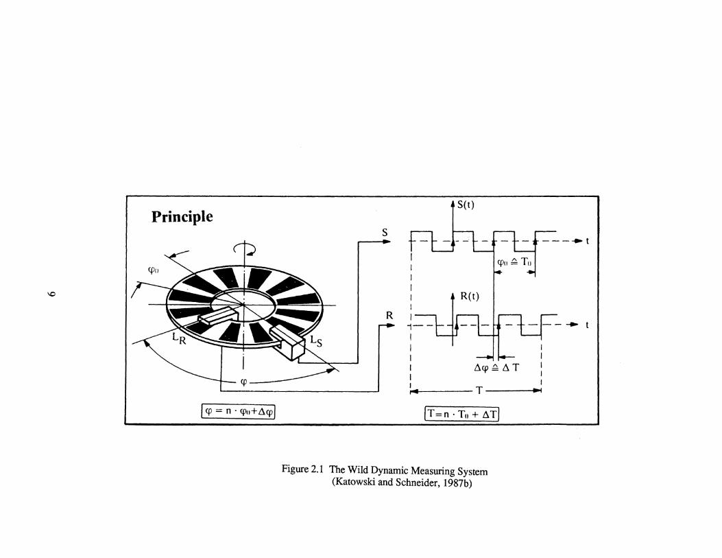
The circles themselves are glass with a radius of 26 mm and are divided into 1024
uniformly spaced sections. Each section contains a line of reflective material which covers
half of the section while the remaining half is left transparent. There are four sensors or
light barriers (as Wild calls them) located around the edges of each circle. Each sensor
consists of an infrared light emitting diode and a receiving diode. Two of the sensors,
describing the zero of the theodolite (horizontal circle) or the zenith (vertical circle), are in
fixed locations on diametrically opposite sides of the circles. The remaining two sensors,
also diametrically opposite each other, revolve around the circles with the alidade
(horizontal) or telescope (vertical) and define the spatial direction of the telescope. Figure
2.1 illustrates the location of just two of the sensors positioned around the circle with Ls
being one of the static sensors and LR one of the revolving sensors, but each of the
remaining two duplicate sensors, as mentioned previously, would be located diametrically
opposite its complement. This method of defining the angle requires that the revolving
sensors LR be capable of passing freely by the static sensors Ls, therefore, each type is
located on opposite edges of the glass circle (LR inside edge and Ls outside edge) as
shown in Figure 2.1.
The angle to be measured is labelled in Figure 2.1 as <p and contains a certain number
of full sections n, each of angle <p 0 , and a partial section, of angle t1<p, which gives the
simple relationship in equation (2-1).
<p = n • <i>o + l1<p (2-1)
This equation is analogous to that involved in distance measurement with an EODM only
now the quantities are angular instead of wavelengths. Two different frequencies must be
measured, a coarse and a fine measurement, to resolve the two unknowns, n and t1<p
8
Principle
\0
I q) = n · cpo+~cpj
s
I I I I I
S(t)
R(t)
R I 1--1 I I I ~cp ~ ~ T I I ,_. T 111>4
IT=n · Tn + ~Tj
Figure 2.1 The Wild Dynamic Measuring System (Katowski and Schneider, 1987b)
--- .... t
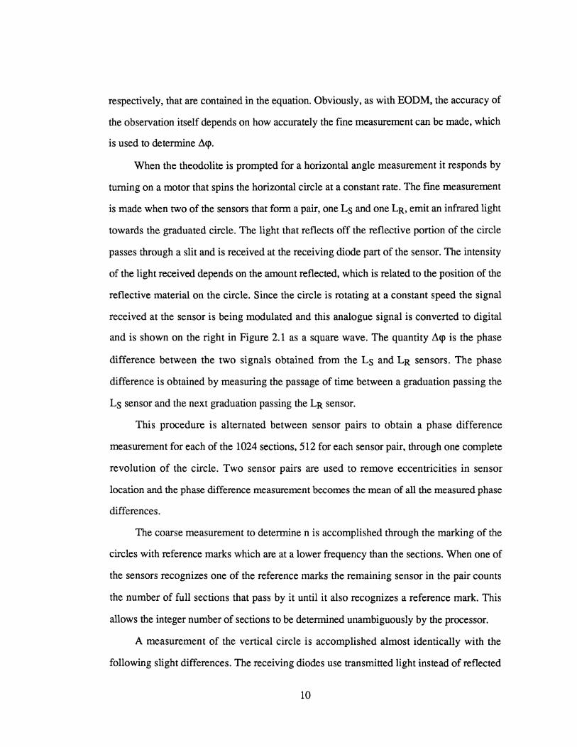
respectively, that are contained in the equation. Obviously, as with EODM, the accuracy of
the observation itself depends on how accurately the fme measurement can be made, which
is used to determine .1<p.
When the theodolite is prompted for a horizontal angle measurement it responds by
turning on a motor that spins the horizontal circle at a constant rate. The fme measurement
is made when two of the sensors that form a pair, one Ls and one LR, emit an infrared light
towards the graduated circle. The light that reflects off the reflective portion of the circle
passes through a slit and is received at the receiving diode part of the sensor. The intensity
of the light received depends on the amount reflected, which is related to the position of the
reflective material on the circle. Since the circle is rotating at a constant speed the signal
received at the sensor is being modulated and this analogue signal is converted to digital
and is shown on the right in Figure 2.1 as a square wave. The quantity .1<p is the phase
difference between the two signals obtained from the Ls and LR sensors. The phase
difference is obtained by measuring the passage of time between a graduation passing the
Ls sensor and the next graduation passing the LR sensor.
This procedure is alternated between sensor pairs to obtain a phase difference
measurement for each of the 1024 sections, 512 for each sensor pair, through one complete
revolution of the circle. Two sensor pairs are used to remove eccentricities in sensor
location and the phase difference measurement becomes the mean of all the measured phase
differences.
The coarse measurement to determine n is accomplished through the marking of the
circles with reference marks which are at a lower frequency than the sections. When one of
the sensors recognizes one of the reference marks the remaining sensor in the pair counts
the number of full sections that pass by it until it also recognizes a reference mark. This
allows the integer number of sections to be determined unambiguously by the processor.
A measurement of the vertical circle is accomplished almost identically with the
following slight differences. The receiving diodes use transmitted light instead of reflected
10

light to carry out the fine measurements. The reason for using transmitted light is to
facilitate the process of correcting the vertical circle measurement for instrument
mislevelment by passing the light through a liquid compensator. The compensator is a vial
filled with a low viscosity silicone oil located between the emitting and receiving diodes of
the sensors. In the T2000 only the vertical circle measurement is corrected for mislevelment
due to the single axial determination, in line of sight direction, of the residual tilt of the
instrument. However, in the latest models, T2002 and T3000, a biaxial method of
determining mislevelment is incorporated allowing the horizontal measurement to be
corrected as well as the vertical.
The time required to complete a measurement of both the horizontal and vertical
circles is approximately 0.9 seconds (s). This can be broken down into 0.3 s for the motors
controlling the circles to gain measuring speed, 0.3 s to process the horizontal circle
measurements, and an additional 0.3 s to process vertical circle measurements as the same
processor is used for both. The least count displayed by the instruments is 0.01 milligons
(mgons), however, testing of the T2000 has revealed this value could be 0.05 mgons
(Katowski and Salzmann, 1983).
A more detailed treatment of the procedures outlined above as well as some testing
results on the T2000 may be obtained from Katowski and Salzmann (1983) and Katowski
and Schneider (1987b), which is where most of the above discussion originates.
2.1.2 The Kern Static System
The original measurement system on the early E1 models has undergone some minor
changes, mostly involving the use of better electronics, for converting analogue signals to
digital. However, on the most part the system has remained unchanged since its inception.
As with the Wild system, it requires the measuring of both a coarse and a fme measurement
11

Brightness distribution
Diodes
Diodes
Ptiase angle
Resultant voltage - -ul - u3 = U1sinf-u3sin(f+l80°) = (U 1+U3)sin.f
min. max. min.
2 3 4 I
f+l80°
(U 1+U3)sinf -=---=----= = tgf (U2+U4}cos.f for U1=U2=U3=u4
-1
Analog signal
- -u2 - u4 = u2sin{f+90°) u4s i n{f+270°) = (U 2+U4)cos:P
Digital angular value
Figure 2.2 The Moire Pattern of the Kern Static Measuring System (Munch, 1984)
12

to completely define the observed angle, but is accomplished in a completely different
manner.
The glass circles used in the Kern E2 instruments are 70 mm in diameter and are
graduated with 20,000 radial marks. Each mark or graduation has a width equal to the
spacing between them of 5.5 micrometers (J.Lm), which all together create a grate with a
grating constant equal to the combined width of one graduation and space of llJ.Lm or 0.02
gons (Munch, 1984 ). The E 1 instruments have identical circle diameters but there are
25,000 graduation lines creating a grating constant of 0.016 gons (Kern & Co. Ltd.,
1981). The reading system incorporates optics which are able to superimpose the
graduation marks covering approximately 2 mm on one side of the circle with their
diametrical opposites to increase the reading resolution. During the superimposition process
the graduations are enlarged in such a way as to create a difference of one in the number of
marks superimposed, which has the effect of creating a Moire pattern as shown in Figure
2.2. This enlargement is further magnified by 2x to double the working length of the area
where the measurements are to be performed. The sensors are four photo diodes arranged
in this area side by side with a separation equal to one quarter of the created Moire period,
which separates the period into quadrants.
The fine measurement for obtaining ~cp of equation (2-1) is accomplished statically
by locating the position of the current Moire period, using interpolation, relative to the
sensors. A signal is generated by each of the four sensors corresponding to the intensity of
the light detected from the pattern. The corresponding signal voltages from the sensors are
combined mathematically, as shown in Figure 2.2, to determine the phase offset of the
Moire period, from the first sensor, and the direction of rotation of the alidade (horizontal)
or telescope (vertical). The ratio of the phase offset divided by the pattern's period (21t) is
multiplied by the expansion factor of 0.01 gons for the E2 and 0.008 gons for the E1,
which represents the circle coverage of one Moire period, to determine the fine
measurement value. All four sensors are required to define unambiguosly the phase offset
13

of the pattern due to each light intensity (except the peak intensity) occurring twice within
the period and the differencing between the sensor signals reduces the systematic errors
contained in the individual voltages. The fine measurement and the phase offset are both
passed to the processor to be combined with the coarse measurement to form the observed
angle.
The coarse measurement n of equation (2-1) is obtained quite simply by counting the
number of impulses detected by the sensor as the alidade or telescope is rotated. The
sensors produce a modulated signal that represents the brightness of the Moire pattern,
which approximates a sinusoid. Various electronic modules are used to create a square
signal which has the same zeros as the sinusoid produced by the sensors. Obtaining the
number of full periods is done by counting the number of transitions from negative to
positive of the square wave. This measurement is also sent to the processor to be combined
with the fine measurement.
Once the processor receives the measurements it must determine the direction of
rotation of the alidade or telescope to know whether to add or subtract the coarse
measurement from the running total that it keeps. As stated previously, this is done by
looking at the voltage differences between sensors. An additional task of the processor
occurs if the phase of the pattern is close to 0 or 21t. This task is analogous to using a
vernier scale where the coarse measurement reference mark is just beyond a full division,
but the magnitude of the interpolation scale reading is very large. One full unit must be
subtracted, or added if the conditions stated above are reversed, from the coarse value to
obtain the proper measurement result. The processor accomplishes this by monitoring the
generated square signal and comparing it to the sign of the trigonometric tangent of the
measured phase. If the pattern has been counted the sign must be positive and if not
counted, negative.
A vertical circle measurement is carried out exactly the same as described above. The
only physical difference between the two circles is the initialization. The vertical circle must
14

be referenced with respect to gravity, in the zenith direction, which requires the counter for
the coarse measurement to be zero at a particular inclination of the telescope. This is
accomplished by supplying two reference marks, one fixed and one rotating with the
telescope, which must be rotated by the fixed mark after power up, to initiate the counter
counting. The horizontal counter may be initialized to zero in any orientation. A continuous
running count is kept of the number of full periods, maximum of 40,000 for the E2 and
50,000 for the El for a full circle revolution, that have passed by the sensors since
initialization.
A biaxial and uniaxial liquid compensating system, in the E2 and El respectively, is
employed separately from the angle measuring components allowing mislevelment
corrections to be determined for the vertical circle readings in both the E2 and El and
horizontal circle readings in the E2. The systems use the reflection of an emitted light off
the horizontal surface of a liquid to determine tilts in either the line of sight direction
(uniaxial) or the line of sight and the trunnion axis directions (biaxial), which are only
applied to the circle readings by the processor when an operator controlled switch is
toggled.
If a more detailed representation of the angle measuring system or the liquid
compensators are desired the interested reader is referred to Munch (1984) and Kern & Co.
Ltd. (1985).
2.2 Electronic and Optical-Mechanical Theodolite Characteristics
The electronic theodolite, like its optical counterpart, is constructed mechanically of
three basic assemblies, which are the base, alidade, and telescope. All of the functioning
parts of the instrument are housed within these three basic assemblies. The accuracy
capable of being achieved by the instrument depends directly on how well each assembly
itself has been constructed as well as the overall combining of the assemblies. No feasible
15

v I
I
L ·-L.
.
I v
Figure 2.3 Relationship Between the Three Major Axes of a Theodolite (Deumlich, 1982)
16
amount of electronics can negate the effects of faulty workmanship in these major
components.
The comparison between optical-mechanical and electronic theodolites can be divided
into two separate categories. The systematic effects that are.related to the workmanship in
the assembling of the three major components and the random errors that are associated
with each instrument and observer pair. Each of these topics will be discussed separately.
2.2.1 The Systematic Errors in Theodolite Construction
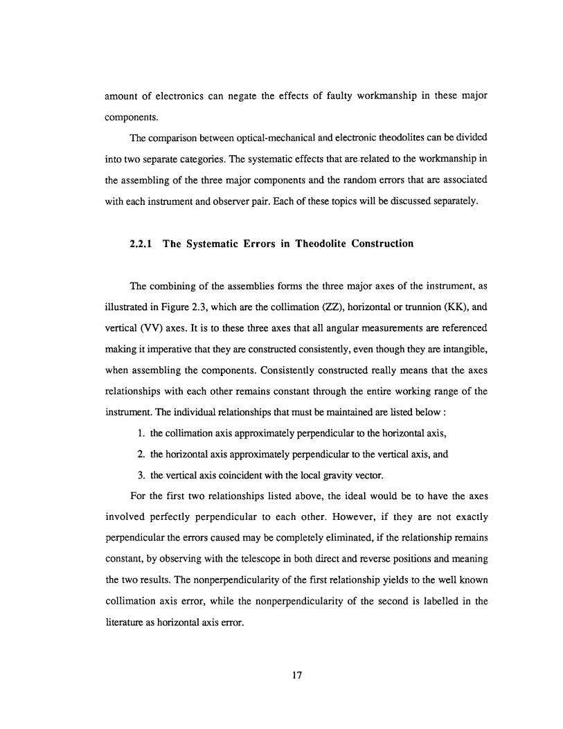
The combining of the assemblies forms the three major axes of the instrument, as
illustrated in Figure 2.3, which are the collimation (ZZ), horizontal or trunnion (KK), and
vertical (VV) axes. It is to these three axes that all angular measurements are referenced
making it imperative that they are constructed consistently, even though they are intangible,
when assembling the components. Consistently constructed really means that the axes
relationships with each other remains constant through the entire working range of the
instrument. The individual relationships that must be maintained are listed below :
1. the collimation axis approximately perpendicular to the horizontal axis,
2. the horizontal axis approximately perpendicular to the vertical axis, and
3. the vertical axis coincident with the local gravity vector.
For the first two relationships listed above, the ideal would be to have the axes
involved perfectly perpendicular to each other. However, if they are not exactly
perpendicular the errors caused may be completely eliminated, if the relationship remains
constant, by observing with the telescope in both direct and reverse positions and meaning
the two results. The nonperpendicularity of the first relationship yields to the well known
collimation axis error, while the nonperpendicularity of the second is labelled in the
literature as horizontal axis error.
17

The third relationship in the list, unlike its predecessors, cannot be removed by
observing in both telescope positions, making it imperative to be able to obtain this
relationship. The relationship may be realized by either perfectly levelling the instrument or
by measuring the amount of residual mislevelment, which is the approach adopted by Kern
in their precision instruments. If the amount of vertical axis tilt can be determined in the
collimation and horizontal axes directions, both circle readings may be corrected,
eliminating this effect. The effect on measurements obtained from the horizontal circle
increases with the inclination of the telescope but are nonexistent with the telescope
horizontal, while those from the vertical circle are constant for each particular line of sight.
This error is known as the vertical axis error or synonymously as the levelling error.
The expected magnitude of the levelling error is related to how well the instrument
can be levelled (i.e. sensitivity of the level vial) and the expected inclination of the telescope
during observations. The following equation gives a general formula for determining the
maximum error in the horizontal circle measurement (crL), due to the mislevelment of the
instrument (Chrzanowski, 1977).
where,
£L error in levelling the vial z is the zenith angle.
(2-2)
The value of £L, when a spirit level is used, is obtained from how well a bubble may be
centered between the graduations of the vial. The levelling error may vary from about
0.02u to 0.2u, where u is the sensitivity of the level vial, depending on the centering
technique used. Thus for u equal to 20" (6.2 mgons), the error of levelling can be between
0.4" (0.12 mgons) and 4" (1.2 mgons). For the liquid biaxial compensator being used on
the Kern E2 a CJL equal to twice the compensator resolution or 0.2 mgon (0.6") irregardless
of telescope inclination can be achieved (Miinch, 1984 ). Similar results are expected from
18

the biaxial compensator now being supplied on the Wild T3000 and T2002 (Wild
Heerbrugg Ltd., 1987).
Traditionally, attempts to randomize the effects of the levelling error, by relevelling
the instrument between sets of observations, has been the approach. The relevelling of an
instrument that has three footscrews (Wild instruments) changes the location of the point of
intersection of the primary axes, which is what defines the theodolite's position. For
industrial metrology applications this is critical, due to the instruments not being centered
over any particular mark, which means that a relevelling would create an entirely different
theodolite position.
Another related error, the index error, is caused by misalignment of the vertical axis
with the corresponding vertical circle zenith. This error is a constant for each instrument
that would have only an affect on the vertical circle measurements, and can be completely
eliminated by observing in both telescope positions. However, if the instrument is
equipped with a liquid compensator, the index error becomes very sensitive to fluctuations
in temperature (Chrzanowski, 1985). Figure 2.4 illustrates the variation in the index error
that can be realized with respect to a change in temperature for both the Kern E2 and Wild
T2000 electronic theodolites. The change in the index error is the result of the relationship
between a variation in the viscosity of the liquid used in the compensators with respect to a
fluctuation in temperature.
This means the index error can only be eliminated, or at least reduced, by observing
either in a rigorously temperature controlled environment or by using both telescope
positions in sighting-to the targets at the shortest possible time interval. An industrial
environment temperature is rarely constant or consistent, due to the varying amounts of
energy released by the large machines involved in a production process, making the second
alternative more plausible. If not removed, a 2" variation in the index error creates a 0.1
mm discrepancy at a 10 m sight distance.
19

Kern E2
4+-~--~----~----~----~----~--~~
2
- -2
~ "CC -6 c ~
-8
-10
-12r-~--~--~-r--~-T----~~----~~--~ 11.5 12 12.5 13 13.5 14 14.5
Time of Day (hr)
Wild T2000
7.5._------------~------------~-----------+
... E
+22.5°C ;-11° C 5 I
2.5
~ -2.5
~ -5 ~ -7.5
-10
-12.5
-15r-~--~--~-r--~~----~--~--~-r--~~ 11 12 13 14 15 16 17 18
Time of Day (hr)
Figure 2.4 Variation oflndex Error with Temperature (altered Chrzanowski, 1985)
20
The above discussion clearly displays a lack of reference to any electronic
components indicating that the errors involving the axes are purely mechanical and will
occur in any type of theodolite. However, electronic modules make the vertical axis error
easier to measure and to apply the proper corrections. Additional errors are inherent in
every theodolite involving eccentricities and circle graduation, which is where the
electronics are involved.
The eccentric errors are created by the components that must rotate around or intersect
with the vertical and horizontal axes of the instrument. For example, a collimation axis
eccentricity is created if the three instrument axes do not all intersect at a common point and
a graduation eccentricity results if the horizontal circle does not rotate symmetrically around
the vertical axis. These eccentric errors may all be completely eliminated by observing with
the telescope in both positions and averaging the two results.
In addition, the graduation eccentricities may be removed by observing diametrically
opposite sides of the circle while the telescope remains in the same position. Optical
theodolites with micrometers accomplish this by using graduation lines from opposite sides
of the circle that must coincide to achieve a fine measurement. The Kern electronic
theodolite deals with this in a similar fashion by superimposing diametrically opposite sides
to create the measurement pattern. Wild in its electronic theodolites has chosen to use
sensors located diametrically opposite each other to negate the effects.
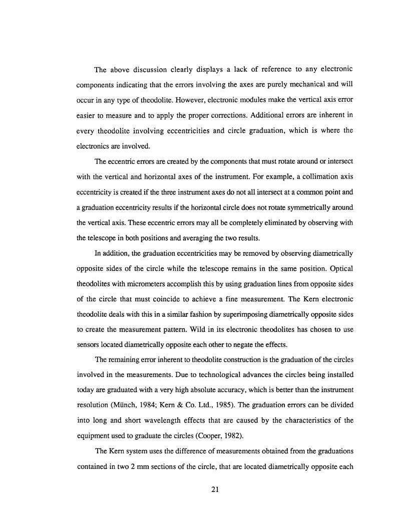
The remaining error inherent to theodolite construction is the graduation of the circles
involved in the measurements. Due to technological advances the circles being installed
today are graduated with a very high absolute accuracy, which is better than the instrument
resolution (MUnch, 1984; Kern & Co. Ltd., 1985). The graduation errors can be divided
into long and short wavelength effects that are caused by the characteristics of the
equipment used to graduate the circles (Cooper, 1982).
The Kern system uses the difference of measurements obtained from the graduations
contained in two 2 mm sections of the circle, that are located diametrically opposite each
21

other, to obtain the final measurement result. The use of only 4 mm of the entire circle
perimeter (70 mm diameter) makes the Kern system susceptable to the effect of the long
period graduation errors, while removing the contributions of the short period errors. In
contrast, the Wild system averages the individual measurements taken over the entire
circumference of the circle, to obtain the final result. This makes the Wild system free from
the effects of both long and short period graduation errors. However, the dynamic
approach of the rotating circle creates a constant speed error that is similar in magnitude to
the graduation errors. As for the optical instruments, using just two graduations
(diametrical opposites) to determine the angular quantity would be a very dangerous
practice to rely on. For both the Kern and the optical instruments, the traditional time
honoured method of using a different portion of the circle for each set, to randomize the
effects of the graduation error, should still be adhered to.
Before closing this section it should be pointed out that there are calibration
procedures for determining the magnitudes and correcting the various theodolite errors that
have been mentioned. The above discussion points out that if proper observing procedures
are followed and the theodolite is mechanically sound, good results will follow, without
having to adjust the instrument. However, the one exception to this statement will be
caused by the inability to level the instrument to a high degree of accuracy or if applicable,
to determine the magnitude of the mislevelment components. If the reader is interested in
the various calibration techniques the literature is boundless and to start the reader is
directed to Deumlich (1982), Kissam (1962) and Faig (1972)
2.2.2 The Random Theodolite Errors
The only remaining errors to discuss involving the theodolites are the random errors
associated with the observer. A determination of the total magnitude of the various random
observing errors, gives a priori information on the accuracy capabilities of a theodolite and
22

observer pair. These errors have been traditionally divided into the categories of reading,
pointing, centering, and levelling, of which the last was discussed in the previous section.
The pointing error of an instrument is a function of the magnification of the telescope
(M) and a constant related to the length of the sight distances. Other factors such as target
design, refraction, and focussing influence the random pointing error ( <1p ). In general, the
following formula gives a good estimation of O'p, for short sight distances of a single
pointing in stable atmospheric conditions including some residual refraction errors
(Chrzanowski, 1977).
op= 30" /M (2-3)
where,
30" = 30 arcseconds.
In most cases, the constant in the above equation can be a little conservative for industrial
metrology applications, where there is usually better control of refraction, target design and
the sight distance rarely exceeds 20 meters. However, to remove any chance of being
overly optimistic this value should be adhered to in computing the expected accuracies,
which translates into a ap of 0.29 mgons (0.94") for the Kern and Wild precision
theodolites, that do not have the panfocal telescope. Both the Wild T2000S and T3000 are
equipped with the panfocal telescope, which has the attribute of being able to change
magnification with changes in sight distance and still maintain an accurate line of sight
(Katowski and Schneider, 1987b; Wild Heerbrugg Instruments Inc. 1987). For these
instruments the above op is representative of a 10 metre sight distance.
The random centering error (a c) that is normally associated with plumbing the
instrument over a station, is completely eliminated in industrial metrology applications
where a coordinating system is to be used (see section 3.4.3). This is due to the theodolite
stations being located randomly in the work area and tied to the control by redundant
observations of wall targets. No observations between instrument stations are required
23

unless two instruments are being collimated together to form the datum (e.g. Wild RMS
2000), which still requires no centering if the datum has not previously been defined. This
unique method removes the large contribution of centering error over very short distances,
which normally is a limiting accuracy factor in traditional surveying applications.
The random reading error (O'R) for an electronic theodolite, like the random centering
error, is almost nonexistant because the circles are read with a very high resolution
electronically. The operator only has to issue a command, instead of trying to coincide the
diametric circle graduations as is the case with an optical instrument. The random error for
an optical-mechanical instrument, including the graduation error, is given by equation (2-4)
(Chrzanowski, 1977).
CJR = 2.5 d (2-4)
where,
d is the smallest division on the micrometer scale.
For the electronic theodolites, assuming that the electronics are capable of reading the circle
to an accuracy equal to the instrument least count gives O'R equal to 0.1, 1.0, and
0.01mgons for the Kern E2, Kern El, and Wild electronic theodolites, respectively.
However, laboratory testing of a T2000 has shown a fine measurement resolution for the
Wild system that is 5 times larger, 0.05 mgons (Katowski and Salzmann, 1983), which is
due to the constant speed error described previously.
The total expected random error (O'T) for a direction measured in a single position of
the telescope is given by the propagation of the individual random errors, described above,
which is illustrated in equation (2-5).
(2-5)
Applying equation (2-5) to the various types of Kern and Wild precision theodolites
commonly involved in industrial metrology gives the results listed in Table 2.1.
24

Model
Kern DKM2-A2
DKM2-AM2
E1 3
E2
Wild T22
T20003
T2002 T30004
2
3
4
Table 2.1 Total Expected Error for Theodolites (for a single pointing)
Circle O'Ll O'p O'R O'T
(mgons) (mgons) (mgons) (mgons)
H 0.71 0.29 0.78 1.09 v 0.20 0.29 0.78 0.86
H&V 0.20 0.29 0.78 0.86 H&V 0.20 0.29 1.00 1.06 H&V 0.20 0.29 0.10 0.37
H 0.71 0.29 0.78 1.09 v 0.11 0.29 0.78 0.84
H&V 0.31 0.29 0.05 0.43 H&V 0.20 0.29 0.05 0.36 H&V 0.20 0.29 0.05 0.36
where applicable a telescope inclination of 30 degrees was used, which is not uncommon in metrology and regularly gets much steeper
optical-mechanical theodolites: DKM2-AM has biaxial and DKM2-A has uniaxial compensation, T2 an optically split level vial for removing tilt in line of sight direction, assumes North American version with circles graduated in arcseconds
at initialization the 1'2000 and El can be levelled very accurately (1 ")and (0.2 mgons) respectively using the single axis compensators, but for the rest of the observing session no corrections are made to the horizontal circle readings for any changes in tilt that occur during use
the T3000 has a varying magnification, therefore the pointing error will also vary with sight distance. The value given for pointing error represents a 10 m sight distance
In analysing the results contained in Table 2.1 it becomes very apparent that the
electronic theodolites add much more to the measurement of a direction then just speed and
automation of the data collection. The improvement in the accuracy of a direction is by a
factor of 3 when using one of the electronic theodolites, with the exception of the Kern E 1,
compared with the optical-mechanical single second theodolites. This of course is due to
the absence of operator limitations in reading the circles of the electronic theodolites, as the
remaining errors, O'L, crp, and crc, would be identical for both types of instruments.
25

Another interesting note is that for one set (a direct and reverse telescope position
paintings) of observations the optimum accuracy capable from the electronic instruments
would already be achieved, making multiple sets frivolous in terms of improving accuracy
for metrology applications (e.g. for the Kern E2, <JT would be 0.30 and 0.27 mgons for 1
and 2 sets, respectively). However, for the purpose of eliminating blunders and having
data quality checks the time honoured practice of turning sets should be adhered to. The
interested reader is referred to Chrzanowski (1977), Nickerson (1978), and Blachut et al.
(1979) if a more detailed discussion of a priori error analysis in observations is required.
26


3. General Overview of Traditional Three Dimensional Positioning
The concepts associated with three dimensional geodetic networks have been well
known for centuries. However, traditionally networks have been subdivided into separate
networks for the horizontal and vertical coordinates. This separation was primarily due to
the inability to obtain accurate terrestrial observation data, that contained information on
both the horizontal and vertical, that would allow the establishing of a single three
dimensional network.
The basic observation for vertical networks has been spirit levelling, which contains
no horizontal information and requires the path between adjacent stations to be accessible.
In contrast, the observations for horizontal networks of distances, directions, independent
angles, and azimuths contain very little vertical information and require intervisibility
between adjacent stations. These contrary requirements and characteristics have resulted in
the historical practice of establishing vertical benchmarks along roads and railways, while
the horizontal stations are located on hilltops and mountains. Until recent decades, the
zenith distance (or conversely the vertical angle) was the only observable that contained
strong information in all three dimensions, but the inability to eliminate the systematic
effects of atmospheric refraction reduced its reliability in merging the horizontal and vertical
coordinates.
Since the introduction of EDM in geodetic surveys in the early SO's, making spatial
distances easier to observe, the interest in three dimensional network solutions has grown.
However, as with the zenith angles, the influence of refraction has not been overcome and
still proves to be the limiting factor. In theory, the micronetworks used in industrial
metrology, where spatial distances would be much shorter, could be pure trilateration
networks.(all observables in the network are distances) The measurement of distances to
27

the accuracy required to form a trilateration network would be extremely inconvenient, in
comparison to the measuring of zenith angles with electronic theodolites.
The three dimensional microtriangulation networks used in industrial metrology rely
exclusively on the zenith angle observations for making the connection between the
horizontal and vertical components. In these micronetworks sight distances are kept very
short and usually are never longer than 20 metres. This reduces the systematic contribution
of the refraction effects, however, short sight distances creates reduced observation
accuracy due to large instrument centering errors, which must be eliminated if the required
accuracies are to be obtained. In addition, the effects of gravity and the earth's geometry
have generally been considered negligible in the establishing of most micronetworks. In the
context of industrial metrology, where in general the positional accuracy requirements are
in the order of 0.1 mm, this statement must be revalidated as to whether all of these effects
are still negligible.
3.1 Three Dimensional Coordinate Systems
The introduction of accurate three dimensional data from extraterrestrial positioning
techniques (i.e. VLBI, SLR, GPS, and TRANSin in the last two decades, has resulted in
the reemergence of three dimensional geodetic networks. The principles behind these global
networks can be applied to the micronetworks that are used in metrology, but obviously at
a much reduced scale. However, in order to carry out a meaningful discussion on these
principles, some basic geodetic coordinate systems and parameters must first be defined.
The definitions may be obtained from any book describing the coordinate systems used in
geodesy, such as Vanicek and Krakiwsky (1986), Krakiwsky and Wells (1971), Torge
(1980), and Bamford (1980) and will be reiterated here only for the sake of completeness.
28
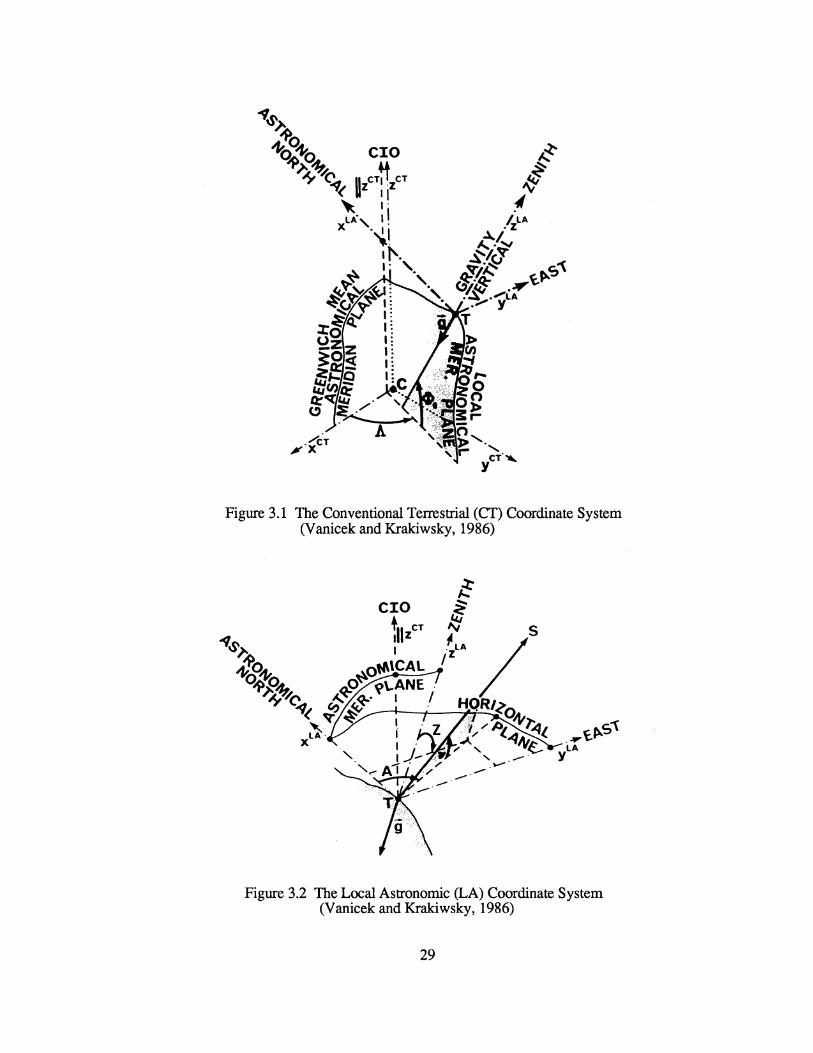
Figure 3.1 The Conventional Terrestrial (CT) Coordinate System (Vanicek and Krakiwsky, 1986)
Figure 3.2 The Local Astronomic (LA) Coordinate System (Vanicek and Krakiwsky, 1986)
29

The Conventional Terrestrial (CT) is the orthogonal coordinate system that is closest
in defining the natural geocentric coordinate system of the earth. The CT system has its
origin at the earth's geocentre (centre of earth's mass). The z axis is defined by the
Conventional International Origin (CIO), the xz plane contains the mean Greenwich zero
meridian (meridian through the Greenwich Observatory) and the y axis is chosen to make a
right handed system. A point T may be defined in the CT system by its cartesian coordinate
triplet (x,y,z)T or its direction, by astronomic latitude and longitude <l>T and AT,
respectively. The relationships between the coordinate axes and astronomic latitude and
longitude are illustrated in Figure 3.1.
The Local Astronomic (LA) is a topographic coordinate system with its origin located
at the position of the observer on the surface of the earth. The z axis, positive outward, is
tangent to the local gravity vector at the point defining the station. The positive x axis points
toward astronomic north which is defined by the z axis of the CT system (CIO), while the
y axis completes the left handed triad. The LA is the coordinate system that the terrestrial
observations are actually performed in. The astronomic azimuth (A) and the zenith distance
(Z) (or conversely the vertical angle (v)) can both be measured directly and are the
parameters that are used to indicate direction in the LA system, to a point of interest, as
given by equation (3-1) and illustrated by Figure 3.2.
(3-1)
The relationship between the LA and the CT systems involve the astronomic latitude and
longitude, that have been defined previously, and this relationship is illustrated in Figure
3.2. The transformation equation, between the two systems, is not required for further
discussions here, but the interested reader may obtain it from any of the above mentioned
literature.
30
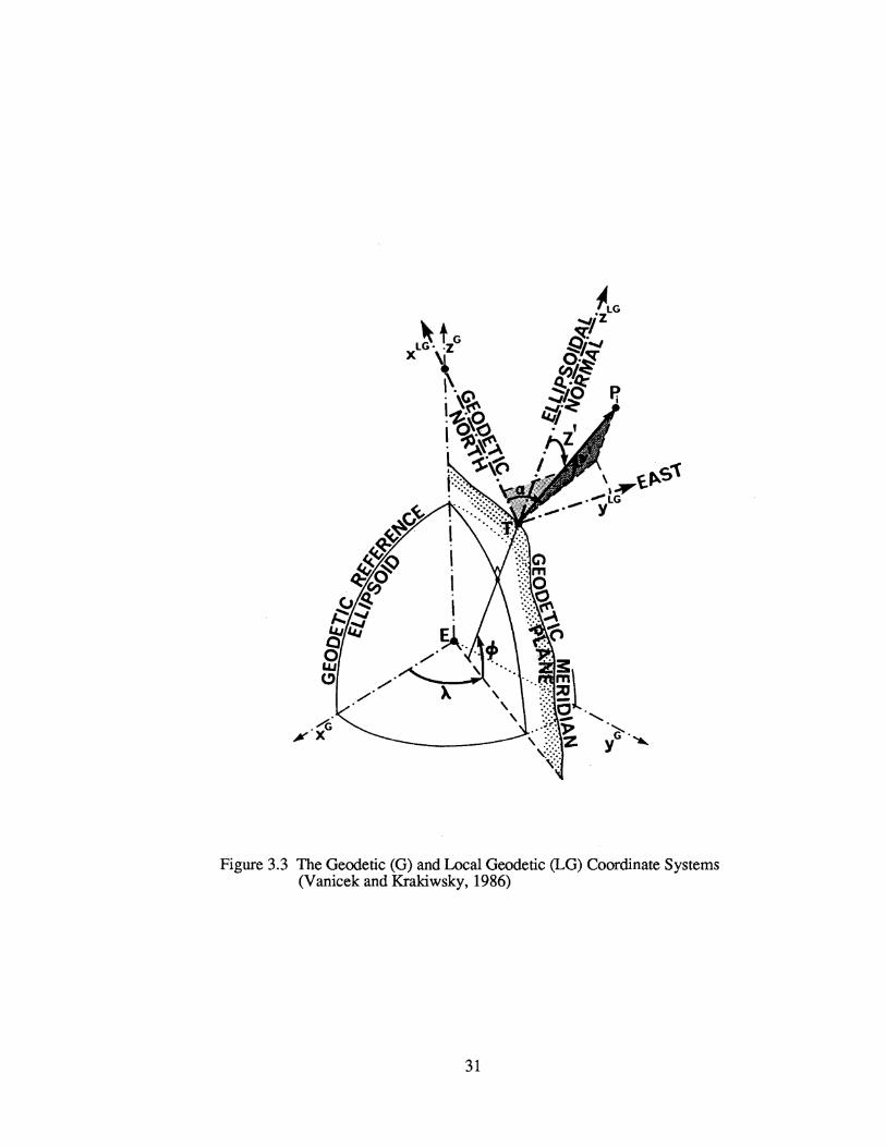
Figure 3.3 The Geodetic (G) and Local Geodetic (LG) Coordinate Systems (Vanicek and Krakiwsky, 1986)
31

The irregular terrain formulating the surface of the earth is very difficult to describe
mathematically, hence, any natural reference surface would also be computationally
complex. Therefore, the simpler model of a "best fitting" biaxial ellipsoid is used (Vanicek
and Krakiwsky, 1986), which forms the basis of the family of geodetic (G) coordinate
systems. The geodetic latitude, longitude and ellipsoidal height, <j), A, and h respectively,
are curvilinear coordinates of a biaxial ellipsoid and are illustrated in Figure 3.3. The
transformation between the geodetic curvilinear to geodetic cartesian coordinates is given
by the following equation (Vanicek and Krakiwsky, 1986):
where,
[ (N + h) cos <j) cos A ] (N + h) cos <j) sin A (N b2fa2 + h) sin <j)
a is the major semi-axis of ellipsoid b is the minor semi-axis of ellipsoid N = a2 I (a2 cos2 <j) + b2 sin2 <j))l/2.
(3-2)
If a geocentric ellipsoid is chosen such that its minor semi-axis is coincident with the z axis
of the CT system and all coordinate axes are coincident with their CT complement, than
equation (3-2) can be utilized to transform directly between the G curvilinear coordinates
and the CT cartesian coordinate differences. For the purposes of this discussion, it will be
enough just to enforce the condition of parallelism and not coincidence between the axes of
the two systems.
The remaining coordinate system that must be defined is the Local Geodetic (LG),
which has a relationship with the G system that is analogous to the relationship the LA has
with the CT system. The LG system, like the LA, is a topocentric system with the origin at
the observer's location and the z axis, positive outward, coincident with the normal to the
biaxial ellipsoid. The positive x axis points toward geodetic north or the z axis of the G
system, which coincides with the CIO in this special case, because of the stipulation cited
32

above for the location of the reference ellipsoid with respect to the CT system. The y axis is
such as to make the LG a left handed triad. The parameters that are required to indicate
direction in this system are the geodetic azimuth (a) and geodetic zenith angle (Z') (or
conversely the geodetic vertical angle (v')), through the following equation and are
illustrated in Figure 3.3.
[ sin Z' cos a ] sin Z' sin a
cos Z'
(3-3)
The relationship between the LG system and geodetic latitude and longitude are also
illustrated in Figure 3.3.
The analogy between the two pairs of coordinate systems described above has
already been referred to and the similarities can be seen very clearly in Figures 3.1 and 3.3.
In fact, if the ellipsoidal normal coincided with the tangent to the actual gravity vector at the
observer's location, the coordinate systems illustrated in Figures 3.1 and 3.3 would be
identical. However, this is not very likely to be the case and the deflection of the vertical is
defined as the spatial angle created by the intersection of the ellipsoidal normal, which
defines the normal gravity vector, and the tangent to the actual gravity vector and is of
particular significance in geodesy. The spatial deflection of the vertical can be further
reduced into two orthogonal components, the prime vertical (11) and meridian (~)
components, which are illustrated in Figure 3.4 depicting their relationships to the LA and
LG systems. With the condition of axes parallelity fulfilled between the G and CT systems,
the simple equations (3-4) and (3-5) are valid in describing the deflection components.
~=<1>-<1> 11 = (A- A.) cos <I>
33
(3-4)
(3-5)

t G illz
.Figure 3.4! The Deflection of the Vertical Components, (altered Vanicek and Krakiwsky, 1986}
An important natural reference smface in geodesy is tne geoid!. which is described! as
tile equipotential surface of the eaFthts ~avity field that best approximates mean sea levet
over tile entire earth (Vanicek and :Krakiwsky, 1986). The local shape of the g~oidi can fue:
characterized with respect to the reference eLlipsoid by. determining a station's surface
deflection components-, which approximate the slope of the geoid in the prime verticali and
meridian directions. In addition, the geoidal height (or undulation) is used to describe the
separation between the geoid and the reference ellipsoid.
3.2 The Terrestrial Observation Equations
As was mentioned previously, the LA system described above is the natural system
that the terrestrial observations are actually performed in. A natural extension to this
statement would be that the observation equations must be greatly simplified if formulated
34

in this system and indeed, this is the case. Unfortunately, the North American convention
for a coordinate system, in contrast to the previously defined LA system, is right handed
with the positive Y axis pointing towards north, which will be introduced as the LA'
system.
The relationship between the LA and LA' systems is simply a reflection of they axis
(to make a right handed system) and a rotation around the z axis to switch the locations of
the x and y axes. The physical meaning of the LA system is not changed, but only the
description of the horizontal coordinate axes. Therefore, to help simplify the discussion and
conform with North American convention, the observation equations will be formulated for
the LA' system. However, it should be pointed out that they may be formed in any one of
the four previously defined coordinate systems by simply accounting for the mathematical
relationships that describe the coordinate transformations between systems.
The azimuth, direction, and angle observation equations are all very closely related to
each other, hence, will be discussed as a unit. Firstly, the function showing the simple
relationship between the cartesian coordinates of the LA' system and an azimuth
observation is given by equation (3-6).
(3-6)
where,
the subscripts i and j represent the at and to stations, respectively.
A simple rearranging of the terms and the addition of a residual component (r) gives us the
observation equation (3-7) that is explicit in terms of the observed quantity, A.
r + Aij = arctan [(xj - Xi) I (Yj - Yi)] (3-7)
A direction observation (d) can be considered the same as the azimuth observation
above with the addition of a term which defines the orientation of the zero mark on the
35

instrument's horizontal circle. Therefore, equation (3-8) depicts the observation equation
explicit in terms of an observed direction.
r + dij = arctan [(xj- Xi) I (Yj- Yi)] - O>i (3-8)
where,
ro is the unknown instrument orientation parameter.
An obvious result of the inclusion of the orientation parameter in the equation is that a
minimum of at least two directions must be observed from each instrument set up, to allow
for the solution of this added unknown parameter.
The orientation parameter may be eliminated from the above observation equation by
simply taking the difference between two direction measurements, to different stations,
from the same instrument set up. The result of this difference forms the observation
equation, explicit in terms of the observation, for an independent angle (~), which is given
in equation (3-9).
r + ~ijk = arctan [(xj -Xi) I (Yj- Yi)] -arctan [(xk- Xi) I (Yk- Yi)] (3-9)
where,
the subscripts i, j, and k represent the at, to, and from stations, respectively.
Up to this point it can be seen clearly by analysing the given observation equations,
for azimuths, directions, and independent angles, that no information has been introduced
concerning the z coordinate (height component in the LA' system). This demonstrates
clearly the need for additional observation types , which will link the x,y coordinates above
with the z coordinate.
The observation equation for spatial distance can be formulated in any coordinate
system simply by forming the expression that gives the defined metric for that coordinate
system, which is usually the Euclidean metric. In the three dimensional space defined by
the LA' system the Euclidean metric, p(i,j), is given by the following equation.
36

(3-10)
The addition of a residual component (r) to (3-10) results in the observation equation for a
spatial distance (s) and is given by equation (3-11).
(3-11)
where,
i and j subscripts represent the at and to stations, respectively.
The zenith distance observation equation can be formulated in two different ways
depending on whether the horizontal or spatial distance between the stations involved, is
used. The formulation given here will be based on the spatial distance due to the regularity
of the cosine function, when the zenith distance approaches 90 degrees. The functional
relationship between the zenith distance and the LA' cartesian coordinates is given by
equation (3-12). cos Zi.j = (Zj - Zj) I Sjj (3-12)
where,
the subscripts i andj represent the at and to stations, respectively.
By simple rearranging, the addition of a residual term (r), and the replacement of the spatial
distance with its cartesian coordinate definition as given by equation (3-11), results in the
observation equation for a zenith distance and is given by equation (3-13).
(3-13)
If alternatively the obs'ervation equation for a vertical angle (v) is required, equation (3-13)
can be used by replacing the. zenith distance term (Zij) with the expression (1t/2- v).
Both observation equations (3-11) and (3-13) have added information linking the x,y
coordinates with the z coordinate of the LA' system. However, it must be pointed out that
the vertical information obtained from a spatial distance is useful only when the lines of
37
sight are steeply inclined. In addition, in the context of metrology networks only enough
distance observations required to alleviate, to a satisfactory degree, the datum scale defect
would be used, due to the inability to determine easily spatial distances to the required
accuracy. In contrast, the zenith distances are easily obtained to the required accuracy and
provide strong vertical information regardless of sight inclination, due to each being a ray
emanating from a point. This illustrates the importance of having good systematic error free
zenith distance measurements, in order to be able to create a three dimensional network for
metrology purposes.
3.3 Variations Between Local Astronomic Coordinate Systems
The review of the observation equations in the previous section was done solely in
the LA' coordinate system. This would be fine if only a single theodolite station were to be
used in the measurements to determine the coordinates of the network targets .. This
obviously will not be the case and is even impossible to accomplish, when distance
observations are not considered, because a target requires at least two intersecting rays to
define its position. However, every network station that is introduced has its own LA
coordinate system, with origin at the station and orientation defined by the station's
astronomic latitude, longitude, and a tangent to the local gravity vector at the station (see
section 3.1).
The traditional approach in micronetworks to alleviate this problem has been to
constrain one of the LA systems from moving (or alternatively a fictitious mean system),
and to solve for translation components (station coordinates), with respect to this fixed
system, for each of the other systems. These constrained methods are quite satisfactory for
most small aperature engineering networks, however, the accuracy requirements for these
applications are not quite so stringent as in metrological networks. These types of solutions
38

give no consideration to the nonparallelity of the complement axes of the various LA
systems, although some is absorbed in the estimated translation components.
The nonparallelity of the complement axes of the LA systems can be broken down
into gravimetric and geometric causes. To obtain an understanding of the magnitude of
each's influence on the overall network results, each will be discussed separately.
3.3.1 Gravimetric Reductions
The relationship between gravity and the various coordinate systems has previously
been established, in section 3.1, with the development of the definition for the deflection of
the vertical. Referring back to Figure 3.4 and the previous discussion on deflection of the
vertical, it should be apparent that the only difference between the LG and LA systems as
defmed in section 3.1, are three small rotations that are caused by the ellipsoidal normal not
being coincident with the tangent to the actual gravity vector at the station. These rotations
have magnitudes that are equal to the values of the station deflection components,~ and T\,
and the difference between the direction of astronomic and geodetic north. The
transformation equation between the two systems is given by the relationship contained in
equation (3-14) (V anicek and Krakiwsky, 1986).
where,
(3-14)
rotation matrices around the x, y, and z axes, respectively
difference between astronomic and geodetic north
are the station deflection components.
39

The small angle between astronomic and geodetic north may be obtained using the
Laplace equation for azimuths. This relationship is given below as equation (3-15)
(Vanicek and Krakiwsky, 1986).
A-a.= Tttan<!> (3-15)
where,
<1> is geodetic latitude.
This simple relationship (3-15) between the two systems only exists because of the initial
condition that was enforced when defining the G system, or the biaxial ellipsoid's position,
with respect to the Cf system (i.e. complement axes parallel).
In the analysis of the above two relationships, (3-14) and (3-15), two characteristics
are very apparent:
(i) changes in latitude affect the definition of the rotation angle caused by the
different directions for astronomic and geodetic norths,
(ii) if the deflection components remain constant in the area, they affect the
transformations from LA to LG identically, excepting point (i) above, for all
stations in the network.
The expectation for the small changes in latitude of a metrology network, point (i), to
have any affect on the transformation is nonexistant, due to the very short sight distances
(usually< 20 metres). However, point (ii) is very interesting, in that it is not the absolute
value of the deflections that is important, but the relative changes in these values throughout
the network. The obvious approach to determining what error contribution the neglecting of
changes in both latitude and the deflection components have, is to compute the differentials
for the above transformation with respect to these parameters. It can be appreciated that all
three rotations are very small, therefore, making a first order approximation of the total
rotation matrix is valid, which gives us equation (3-16) (Vanicek and Krakiwsky, 1986).
40

[ 1 (A-a) ~ ] [ x ] LA
-(A-a) 1 11 Y
-~ -11 1 z
(3-16)
where,
A - a, ~. and 11 are all in radians.
The derivation of the partial derivatives for all three of the variable parameters is
trivial, hence, only the final rearranged differential equations, explicit in terms of the
varying parameters, will be given. Equations (3-17) and (3-18) show the partial derivatives
explicit in terms of a small change aq, in latitude for x andy, respectively (az{<)cp = 0).
a<1> = ax cos2 <1> I 11 y
a<l> = -ay cos2 <1> I 11 X
(3-17)
(3-18)
These equations show very clearly that any small change in latitude can be tolerated
for networks located anywhere on the earth's surface, for all magnitudes of deflection
components, to obtain much less than a tenth of a millimetre for the coordinates involved in
the transformation. For example, expecting an accuracy of 0.05 mm on the equator ( cp = 0°)
with an x or y coordinate of 30 metres and a deflection component of 10", allows for a
change in latitude of almost 2 degrees. This finding is certainly not unexpected and has
only been presented for completeness.
The parameters that are of real interest are the deflection components. the two
equations (3-19) and (3-20) give the partial derivatives explicit in ~ for the x and z
coordinates (ayla~=O), while equations (3-21) to (3-23) are explicit in 11. for the x, y, and z
coordinates, respectively.
a~=axl z a~ = az I -X
a,= ax I ytan<P
a, = ay I (z -X tan <1>)
a, = az I -y
41
(3-19)
(3-20)
(3-21)
(3-22)
(3-23)

A network designed for metrological purposes is very likely to be more dominant in
either the x or y coordinate (if these are the horizontal components), with a maximum z
coordinate almost always less than 10 metres. This results in equation (3-20) showing a
more stringent requi,reJ;Uent for£\~, while the requirements for t\11 is dependent on network
latitude. Figure 3.5 gives an illustration of the maximum allowable deviation for ~ and 11
(as it varies with latitude), while considering a required accuracy of 0.05 mm in all three
coordinates, with a maximum sight distance of 30 metres along either the x or y axis, and a
10 metre z coordinate.
The allowable deviations for both deflection components is in the range between 0.2"
to 0.4" (arcseconds}. Altliough tms at first seems very stringent, one nn1st bare int mindl that
these changes must occur over the sig~l distance of 30 metres•. Due to the namre of tneJ
geoid, which is considered! as a very smooth, always convex surface ~Vanicek andl
Krakiwsky, 1986}, this is not very likely to happen. In addition, the case presented is very
drastic and is also not very likely to occur, which would allow a little more tolerance for
changes in deflection.
-:> ._,
s=" <1
o($·
tJJ' <1
o:
-.5
-1
-1.5 0 10 20 30 40 50
Latitude (deg.)
0 Eqt.(3-19) 0 Eqt.(3-20) • Eqt.(3-21) c Eqt.(3-22) /:,. Eqt.(3-23)
60 70 80 90
Figure 3.5 Maximum Tolerance for Changes in the Deflection ofthe Vertical
42
The relationship between the LA and LG system is more complicated if the axes of
the G and CT systems are misaligned. However, the same theory is still applicable, only
equations for the deflection components and misalignment of astronomic and geodetic
norths are more difficult io obtain. The interested reader is referred to Vanicek and
Krakiwsky (1986), Torge (1980), or Bamford (1980) for a more detailed treatment of this
situation.
3.3.2 Geometric Reductions
With the effects in the variation of actual gravity removed or neglected (if deemed
negligible), the quantity of LA systems forming the network has now been transformed to
an analogous network of LG systems. The complement axes of the various LG systems are
still not parallel, due to each system's definition of the x axes, changes direction with a
change in longitude, and the fact that the systems are located on a curved surface, the
reference ellipsoid. However, the mathematical relationships involving this reference
surface are very regular and well known, making it a trivial task to determine the effects of
neglecting these final reductions.
To simplify the mathematics further a reference sphere will be used in place of the
customary ellipsoid. This is a valid simplification due to the very small area and differential
rotations that are to be analysed. The minimum (rmin) and maximum (rmax) radii of
curvature of the surface of a biaxial ellipsoid occur at the equator and poles and are given
by equations (3-'24) and (3-25), respectively (Krakiwsky and Thompson, 1974).
where,
rmin = a
rmax = a I (1-e2)112
a is the major semi-axis of the reference ellipsoid e2 = (a2-b2) I a2 is the first eccentricity of the ellipsoid b is the minor semi-axis of the reference ellipsoid
43
(3-24)
(3-25)

Station l Meridian fotr Station2
Figure 3.6 Rotation Around the Z axis
Equator
c
Figure 3.7 Rotation Around theY Axis
44

The micronetworks in industrial metrology applications would rarely exceed an aperature of
100 metres. This would translate into an angular variation of only 0.01" between using the
maximum and the minimum radii of curvature, using the biaxial ellipsoid parameters for the
North American Datum 1984 (NAD 84,.a = 6378137.000 m and b = 6356752.314 m).
This small variation is negligible when determining the required rotations, hence, a surface
with a constant radius (a sphere) is a valid simplification for the computations.
Three small rotation angles can be derived from the two triplets of geodetic
curvilinear coordinates (cp, A., h) that define the location of the two LG systems on the
ellipsoid. These rotations represent the misalignment of the three coordinate axes of the two
systems.
The small rotation required around the z axis of the second system, to make the
projection onto a horizontal plane of the remaining two axes parallel to their complements,
is simply the difference in longitude between the two stations (see Figure 3.6). The same
visualization can be used to determine the small rotation around the y axis of the second
system to make the two x axes parallel. This is simply the difference in latitude between the
two stations, as illustrated in Figure 3.7. The remaining rotation, around the x axis, to
bring the remaining two sets of axes parallel is not as easy to visualize. After the
completion of the initial two rotations, the z axis of the second system must be projected
into the yz plane of the first system. Figure 3.8 illustrates the cross section of the sphere
along the YIZI plane, displaying the simple geometry involving the desired rotation angle
(ro), which is given by equation (3-26).
where,
ro = arctan [d I (R +h)] (3-26)
d distance between z axes in the horizontal plane of the fixed LG system R radius of the reference sphere h ellipsoidal (spherical) height of the fixed LG system station.
45

The computed rotation ro is dominated by the magnitude of the sphere's radius, hence, the
distance and the height need only be approximate for this computation.
The three rotations when combined form a single total rotation matrix, that can be
populated by the first order approximation of its components, due to the rotations being
differentially small. Equation (3-27) gives the total transformation relationship, including
the origin offsets, that aligns and brings into coincidence, the complement axes between the
two LG systems.
where,
11/.., 11cj>, and ro x0 , y0 , and z0
(3-27)
are all in radians are offsets of the LG2 origin in the LG1 system.
In micronetworks, the above transformation is usually applied implicitly in the
formulation of the observation equations. The datum is created, as mentioned previously,
by fixing the location of one of the network's LG systems. This fixed coordinate system is
translated, maintaining orientation, to the remaining network stations, to obtain offsets
describing the origins of each of their systems with respect to the one fixed system. The
vectors, describing the observed quantities, are then formulated into observation equations
by using the offsets determined for each station's origin, in place of the coordinates defined
by the instrument location's LG system.
This procedure c?mpletel~ eliminates the effects of the misrotation (M, 11<!>, and ro)
and horizontal offsets (x0 and y0 ) of the various systems, as described in equation (3-
27).However, tacitly assumed in the procedure is that all of the stations involved in the
network can be described by simple translations. For this assumption to hold, all of the
planes formed by the tangents to the earth's surface, at each of the network stations,
would have to be parallel. Unfortunately this is not the case, as the network is being
46

LG Zt
Great circle in . w the 'VZ ~ plane
Figure 3-.8 Rotation Around tlle X Axis
Figure 3.9 The Effect of Neglecting Earth Cwvature
47

formed on a curved surface.
The invalid assumption is reflected in the vertical offset (Zo), of equation (3-27), not
being completely eliminated in the formulation of the observation equations. The effect is
given in equation (3-28) (Faig, 1972) and illustrated in Figure 3.9, which also show that
the magnitude of the expected deviation, will increase with distance away from the fixed
LG system.
(3-28)
where,
Ah the error in height caused by neglecting the earth's curvature d distance from fixed LG system R radius of earth.
A vertical error of 0.1 mm can be introduced, with only a 36 metre distance from the fixed
system!
In most metrology applications this probably can be neglected due to the relative
smoothness being the more dominant criteria then absolute heights. However, there are
some applications that require absolute alignment, in which case this correction must be
considered.
3.4 Design Criteria for Metrology Micronetworks
The last topic to discuss concerning three dimensional networks, are the peculiarities
that are associated wit~ metrology networks in particular. These networks are of the highest
possible order, therefore, need some special considerations in their design as well as
measurement. In particular, these considerations are scale, horizontal and vertical
refraction, and the removal of the random centering error associated with angular
measurements.
48

3.4.1 Scale Determination
Scale determination in a metrology network is a very interesting problem. Typical
engineering networks h~ve a minimum aperature of 1/2 kilome.tre and are usually larger
than this (1 to 2 km). This allows distances to be measured randomly throughout the extent
of the network or even possibly to define the entire network (trilateration). There are many
portable EODM 's being manufactured that allow distances to be measured, in networks of
typical aperature, between 0.5 mm to 3 mm accuracy depending on the type of instrument
used. A properly calibrated EODM has proven to be a very successful method of alleviating
the scale defect in these networks. However, this same methodology cannot be carried over
to metrology networks of a few tens of metres distances, primarily because of the inability
to measure the short distances accurately enough (say 0.05 mm) to satisfy the scale
requirements.
The only real solution to this problem is the use of calibrated scale bars. The two
targets that define the scale bar length can be tied to the network through triangulation, with
the known distance between them added as a spatial distance observable. This method
eliminates the scale defect in the network, but in doing so creates some additional concerns.
The scale bars themselves must be constructed of some very environmentally stable
material, such as invar, to ensure no systematic change in length while being used. The
absolute length determination of the bars requires the use of an interferometric comparator,
which in practice will only be able to obtain the length to an accuracy of± 0.01 mm, due to
the difficulties in optical identification of the centres of the attached targets. For a 2 metre
scale bar, this already would create a systematic scale error of 5 ppm in the network. This
scale error could be reduced by using a longer scale bar, however, this creates logistical
problems in transporting and in some cases calibrating, due to the limits of some calibration
interferometers.
49

Of primary importance when using scale bars, is the way in which the scale
associated with them is propagated into the network. A chapter can be taken from the
geodesists of the past, who created triangulation networks using a single measured baseline
for scale (Bomford, 1980). Their techniques were designed for horizontal networks, which
is where the concern for scale exists in metrology networks. The height component usually
has a much smaller working range, which would probably never exceed a few metres
making systematic scale error much less of a problem. However, it is critical to create a
reasonable working range in height, not having all stations located in almost the same
horizontal plane, to achieve good solutions for this component.
3.4.2 Atmospheric Refraction
The systematic effects of refraction have already been alluded to at the beginning of
this chapter. The usual approach to the lessening of the vertical refraction effects, in
traditional networks, is by observing simultaneous zenith distances between the two
stations. This is not possible to accomplish in metrology networks, where the bulk of the
stations are wall targets. In addition, the centering error created by such a procedure would
likely overshadow the effects that are to be removed. In addition to vertical refraction,
horizontal refraction must also be considered in the confmed areas of metrology networks,
where the positioning of instrument stations may be dictated by the space available.
The only real solution to the refraction problem is to try to keep the effects to a
minimum through the design of the network. If the sight distances are kept very short(< 20
metres) and lines of sight are kept from going close to large bulky apparatus (i.e. large
machinery, hanging fixtures, jutting walls, etc.), which may produce heat radiation, most
refraction effects can be eliminated. Additional considerations are required for sight
directions, if the network is being designed to monitor components involved in a working
production process. These processes generally produce a lot of energy which will create a
50

very inhomogeneous atmosphere. An attempt should be made in the design of the network
to eliminate sight directions, if possible, that go over top or close by the sides of any
processes that release large irregular quantities of heat energy into the air.
Temperature gradients affect optical light rays by bending them, creating a curved
line of sight path. This means that the actual circle readings are with respect to the tangent
to the curved path at the instrument station, instead of the required straight line path. The
following equation can be used to compute the horizontal error ("() in the line of sight
direction due to lateral refraction (Blachut et al. 1979).
where,
1· = 8.0 .. [~J [m (3-29)
p T s dT/dx
is the barometric pressure in millibars is the temperature in kelvin degrees (T = 273.15 + t in °C) is the sight distance in metres is the horizontal temperature gradient, perpendicular to the line of sight.
For a 0.1 mm lateral refraction error to occur over a 20 metre sight distance, would require
that the tangent to the line of sight at the instrument station deviate in the horizontal plane by
1" from a straight line of sight. From equation (3-29), assuming standard pressure and
temperature, a horizontal temperature gradient of 0.5°C/m is all that is required to create
this deviation in the line of sight. A gradient of this magnitude can occur if large quantities
of heat radiation are being produced
The temperature gradients could be measured to correct the circle readings for the
refraction effects. However, it would be very impractical and difficult (could change many
times over a single line of sight) to measure the temperature gradients for various lines of
sight. The only real solution to the problem of refraction is to try to minimize the effects by
keeping the temperature distribution constant within the work area (i.e. keep doors and
windows closed, switch off machinery, etc.).
51

3.4.3 Centering Error
The remaining consideration for metrology networks is the removal of the random
centering error contribution to.the observed quantities. This too, has been alluded to at the
beginning of this chapter, and also was mentioned previously in section 2.2. In traditional
engineering networks this error has been reduced by developing forced centering methods,
which reduces the contribution of centering error to ± 0.1 mm. In addition to not meeting
the requirements for metrology, these methods require stationary pillars to be constructed at
the network stations. This is obviously not suitable for use in metrology, where instrument
locations must be located very close to the components being set out or monitored.
If the datum has not been predefmed, the precise physical location of the instruments
is immaterial and the actual centering can be ignored. The instruments would not have to be
physically centered over a mark, but the precise relative positions between the instruments,
in some common coordinate system, would have to be determined. The spatial line
connecting the intersection points of the primary axes of each theodolite (see Figure 2.3)
can be used to create the reference system. Each instrument can be treated as a combined
collimator and telescope, and by using a special technique for sighting on the crosshairs of
each instrument (Kissam,l962), the two lines of sight created by each telescope can be
brought into coincidence.
Although the above approach solves the relative location between instruments, there
are some problems associated with it. The procedure used for the alignment can be quite
tedious and time co'nsuming, unless the instruments are specially equipped with targets
defining the intersection of the horizontal and vertical axes (e.g. the Wild T2000S). The
relative orientation that is established between instruments is determined uniquely, with
nopossibility to create any redundancy in the solution. In addition, there are severe
limitations for extending the reference system to other theodolite locations, due to the
accumulation of error for the collimation techniques. The methodology is very cumbersome
52

0' Theodolite Station
D' Wall Target
Figure 3.10 The Method of "Free Positioned" Theodolite Stations
53

to use when the network is being densified or extended, quite possibly making the
centering over marks necessary to maintain the datum, which certainly would reduce a
coordinating system's accuracy capabilities.
However, the above limitations can be eliminated by using a unique characteristic of
metrology networks, that allows the random centering error for each instrument station to
be completely removed from the solution. The instrument station locations themselves are
not the main concern when establishing the network. It is the locations of the reference wall
targets that are the primary objective, with the instrument locations serving only as a link
between the different wall targets. This means that the precise physical location of the
instrument centre is immaterial as long as it fulfills the designed geometric criteria for the
network.
Therefore, if observations between instrument locations are not performed, the
instruments can be randomly located in the general vicinity that was designed, with no
thought of having to centre over a particular physical mark. The redundancy that is lost by
not observing between instrument stations is restored by observing redundant rays to the
wall targets. The coordinates of the instrument locations can be thought of as nuisance
parameters, which must be added to the network solution in order to obtain the desired
quantities, the wall target coordinates. Of course, how well the coordinates of the wall
targets are determined is related directly to the accuracy of the linking stations, therefore,
great care must still be taken in obtaining good solutions for the instrument coordinates.
This approach is analogous to that employed in the bundle method of aerotriangulation
(Brown, 1985), where the perspective centres of the different camera locations are
determined, only to obtain the link between ground stations. Figure 3.10 shows a typical
scheme of direction observations in establishing a reference microtriangulation network
using the method of the "free positioned" theodolite stations.
54

4. Algorithms for Coordinating System Software
The integration of a coordinating system with traditional metrology methods gives the
ability to determine coordinates, offset values, corrections, surface coefficients, or whatever
is required in virtual real time. This is the major advantage that the system provides, in
comparison with the traditional optical-mechanical methods. A disadvantage of the
coordinating system is that the parameters needed in the setting out or maintenance surveys
are not directly determined, but have to be derived from coordinates. Therefore, as already
alluded to in the introduction, it takes a great deal of computer software to give a system the
flexibility that is required, for even just a single application of the system.
There are primarily two types of coordinating systems in use in North America, the
Wild C. A. T. 2000 and the Kern ECDS2, which together have created a suite of standard
algorithms that are being adhered to in industry. In these algorithms, the basic geodetic
measurement principles that have prevailed in triangulation for centuries, have been replaced
by quicker measuring techniques to lessen the preliminary set up times and to accelerate the
obtaining of the required parameters. The loss in accuracy caused by this substitution can be
tolerated for some system applications, where the optimum achievable accuracies are not
required. However, for any application wanting to use the coordinating systems to their full
potential, this becomes a serious limitation as has been shown in section 2.2, where errors
inherent in theodolite construction have been discussed
This chapter is designed to discuss the major aspects of the software that must be
considered in order to achieve the optimum accuracies available, with a high degree of
certainty in the results. Figure 4.1 illustrates the five main software modules that comprise a
coordinating system. The primary considerations for the development of each of the four
components surrounding the main program module will be discussed. This will be followed
55
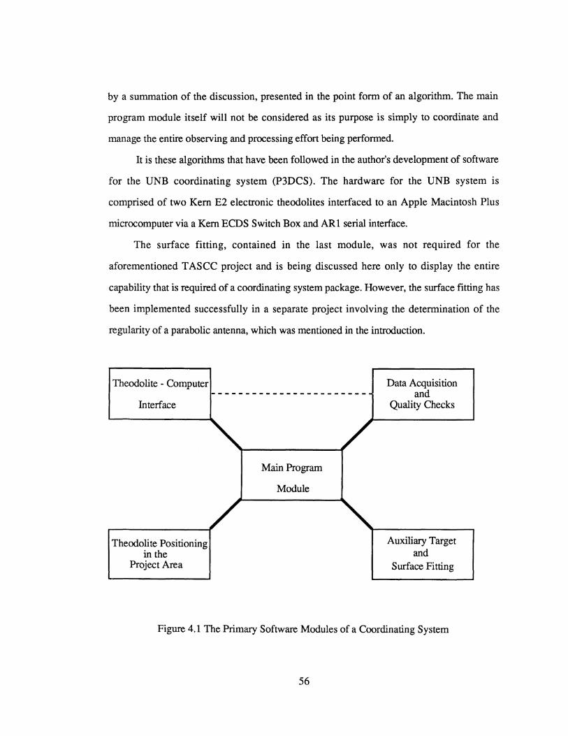
by a summation of the discussion, presented in the point form of an algorithm. The main
program module itself will not be considered as its purpose is simply to coordinate and
manage the entire observing and processing effort being performed.
It is these algorithms that have been followed in the author's development of software
for the UNB coordinating system (P3DCS). The hardware for the UNB system is
comprised of two Kern E2 electronic theodolites interfaced to an Apple Macintosh Plus
microcomputer via a Kern ECDS Switch Box and ARl serial interface.
The surface fitting, contained in the last module, was not required for the
aforementioned TASCC project and is being discussed here only to display the entire
capability that is required of a coordinating system package. However, the surface fitting has
been implemented successfully in a separate project involving the determination of the
regularity of a parabolic antenna, which was mentioned in the introduction.
Theodolite - Computer
Interface
Theodolite Positioning in the
Project Area
Main Program
Module
Data Acquisition and
Quality Checks
Auxiliary Target and
Surface Fitting
Figure 4.1 The Primary Software Modules of a Coordinating System
56

No
Issue Command
Prompt
Get String From the Serial Port
Decode Data Stting
Set Communication 1----~
Protocol
Figure 4.2 Flow Diagram for the Theodolite-Computer Interface
57

4.1 The Theodolite - Computer Interface
The theodolite-computer interface is the module that controls all of the communication
that occurs between the theodolites, computer, and operator issued commands. As such, the
tasks that it must perform involve the setting of the serial port communication protocol,
prompting theodolites for measurements, receiving the data strings, decoding the data
strings, and checking if the decoded values are realistic. No actual data processing is
performed by this module as its sole purpose is to supply the observations in a usable form
to be processed by the remaining modules.
Figure 4.2 illustrates the flow of events that should occur to obtain successful
measurements in one of the telescope positions for all the theodolites involved in the
observing of a particular target. From this illustration the task of the interface can be
subdivided logically into the setting of the communication protocol and the data decoding.
4.1.1 The Communication Protocol
The first step, setting communication protocol, is a direct result of the mode of
communication being serial and obviously is only required to be done once for the entire
observing campaign. This accounts for it being segregated in Figure 4.2 by the dashed line.
The actual setting of the protocol can be separated into two distinct parts that are hardware
and software related.
The hardware component involves the actual physical connection, via cables, between
the theodolites and the microcomputer. The connection is usually accomplished using one of
the many forms of the RS-232 interface, which is dependent on the interfaces employed by
the components being connected, as well as the connector receptacles themselves. The
complement pins contained within the interface, in whatever way they are defined, must be
properly connected (i.e. data transmit of one component with data receive of the other, etc.)
58

in order to achieve successful communication between the devices. It is not the author's
intent to give a detailed discussion on communication using the RS-232 interface, but only to
indicate that it is a critical part of the communication procedure that must not be overlooked.
The pin configuration requit:yd tp complete the interface between the Kern E2 theodolite and
the Apple Macintosh Plus and SE computers is illustrated in Figure 4.3. The maximum cable
length is usually limited by the transmitting abilities of the DC powered theodolites, but is
normally in excess of 100 metres (e.g. the Kern E2 specification is 150m). The reader
interested in obtaining detailed treatment of the pin configuration in the RS-232 interface is
referred to Campbell (1984).
The remaining component, software, of the setting of the communication protocol
deals entirely with the description of the data being transmitted between the devices. Each
device must know what to expect from the other before any meaningful communication can
occur. The defining characteristics of a data transmission are the baud rate, bits per character
(data bits), number of stop bits, and parity.
DIN5 DB 25 Connectors
Male Female 1
-Kern ASB (LEMO FG.OB) to Epson HX-20 (DIN 5)
Kern ASB-RS-232 AR1 (part no. 115.508.725 6)
2 35041 Male DIN 5
Apple Imagewriter I cable connected to the modem port
Figure 4.3 The Macintosh Plus/SE - Kern E2 Interface
59
I
The theodolites have these parameters fixed at specific values (e.g. Kern E2: 1200
baud, 7 data bits, 2 stop bits, and even parity), which requires that the computer have to
conform its serial'port to the.,.needs of the instrument. This is accomplished by using
software to open the serial port, much like opening a file, with the specified communication
parameters. Normally the serial port must be opened twice, once each for input and output,
as each is really a separate operation not directly involving the other.
No algorithm will be presented for the software portion of the communication
protocol. The approach for software development is dependent on the computer
manufacturer's considerations in developing the serial communication port, as well as the
type of programming language being used for the software development.
4.1.1 The Data Decoding
Once communication has been established between the theodolites and computer, the
primary task of the interface module becomes that of a provider. As such, this portion of the
interface is very closely related to the data acquisition module, which is illustrated by the
dashed line joining the two in Figure 4.1. The interface must be able to issue the proper
measurement commands and provide the observations in a usable form for processing at the
data acquisition stage.
A measurement prompt consists of a string of ASCII command characters that are
transmitted to the theodolite, which when interpreted begin the electronic measurement of the
horizontal and/or vertical circles. As would be expected, each theodolite manufacturer have
their own command characters as well as calling sequences. The following string of
characters (with hyphens and spaces removed), STX- T- 2- 1 - 1 - 2- CR- Lp, illustrates a
command string that would prompt a Kern E2, with J.D. set to 2, to measure and transmit
both horizontal and vertical circle readings. ·
60

The retrieved transmission from the Kern E2 would be an ASCII variable length record
with all trailing and preceding zeros in the circle measurements not being transmitted (e.g. a
horizontal circle measurement of 1.2 gons would be transmitted as 11 + 1.2). The following
character string, ll+HHH.HHHH 12+ZZZ.ZZZZCRLF, illustrates the format for the
maximum length record that would be received using the previously described command
string for the Kern E2 theodolite.
Once the data string has been obtained from the serial port the only remaining task of
the interface is to decode the string and check if decoded values are realistic, before handing
them over to the data acquisition module. The decoding itself is very straight forward,
however, different decoding routines are required for the different manufacturer's theodolites
due to the variation in data string formats. The check on the decoded values is simply to
ensure that either the command or data strings have not been corrupted in the transmitting
process by electronic glitches, voltage surges, environmental effects, or whatever. The term
realistic simply means that the values decoded are within the measurement range of the
instrument (i.e. between 0 and 3600 for angular measurements). If the values are not deemed
realistic the command to measure should be repeated and new values decoded before control
is released back to the data acquisition module.
In summarizing the above discussion and referring to Figure 4.2, the following simple
algorithm is obtained, which has been conformed to by the author in the development of
software for P3DCS.
1. Determine if the operator(s) is/are ready to have the measurements performed.
2. Issue the appropriate measurement prompt string of ASCII command characters.
3. Determine when the input data string has been received at the serial port.
4. Obtain the string from the serial port input buffer and decode it into the separate
observables (i.e. horizontal direction and zenith angle).
5. Determine whether the values are realisticly possible (i.e. have not been corrupted).
If the values are in doubt, return to step 2.
61

6. Detemrine if all the instruments involved in the measurements to this target have
been prompted. If not, go back to step 2. and repeat the process for the next
instrument. If they have, return to the data acquisition with the results.
Although only examples for the Kern E2 theodolite have been presented, the Wild
system is very similar and can be handled in the same way. For more information regarding
the two systems, character commands, and instrument response, the interested readers are
referred to Kern & Co. Ltd. (1984a) and Wild Heerbrugg Ltd. (1984) for the Kern and Wild
electronic theodolites, respectively.
4.2 Data Acquisition and Quality Checks
There is no mystery behind the data acquisition and quality check module, its primary
functions are as its name suggests. Its tasks are to acquire the observations complete with
station names, perform a station adjustment (if more than one set of observations is made),
and provide a reliable filter for quality control. All obvious blunders, mispointings,
electronic glitches, and misspelled station names must be eliminated from the data set
before control is passed back to the remaining modules. Figure 4.4 illustrates the flow of
events that should occur in this module to ensure a reliable data set.
The traditional geodetic methodologies that are normally used in triangulation
networks are employed for the data acquisition. This requires that targets be observed in
both direct and reverse telescope positions with the well established rules for measuring
sets and pointing order within a set being adhered to. The measuring of both telescope
positions ensures that the systematic errors inherent in theodolite construction are
eliminated, or at least made negligible, from the observations (see section 2.2). This is
critical if the coordinating system is being used to obtain the optimum possible accuracies
as there cannot be a trade off between accuracy and the speed at which the required
parameters are obtained.
62

Detennine the measurements to be repeated
No
Get# of sets &
# of targets/set
Give the station I.D.
Theod-Comp Interface Module
Compute & nonnalize coli. & index errors
Compute means & discrep. for
each line of sight
Yes
Get the station I.D.
Edit target
I.D.'s
Compute new
set means
Figure 4.4 Flow Diagram for the Data Acquisition Module
63

The index error and the true collimation error for each instrument are unique and
should remain constant for each set, and as such provide a very good assurance of data
quality. The true collimation error can be defined as the angular amount that the collimation
axis (optical axis) and the horizontal axis (trunnion axis) deviate from perpendicularity with
the instrument telescope having zero inclination. The use of the true collimation error as a
consistency check, requires that the derived collimation error from the measurements be
modelled for the effects of telescope inclination. The functional relationship to determine
the true collimation error (c) from that derived from the measurements (c') and the telescope
inclination (y) is given by equation (4-1) (Cooper, 1982).
c = c' I cos"( (4-1)
The index and true collimation errors are only made available due to the observing of
the observations in both telescope positions, which gives even more criteria for following
the traditional geodetic approach. In addition, the liquid compensators employed in the
instruments are very sensitive to temperature changes (see section 2.2) making the index
error very temperature dependent. The index error can change by several arcseconds within
a single set of observations, which makes it imperative to monitor changes in its magnitude
to detect and remove the possible systematic effects.
The remaining constituent in the quality control ftlter are the discrepancies that can be
computed by redundantly observing targets from the same instrument station. The
discrepancy between the mean of the two telescope positions for an observation in the
current set and the mean value for the same quantity from all previous sets, can be easily
derived. There are two possibilities if a discrepancy is found to be beyond the acceptable
limit. If the true collimation or index error, depending on discrepancy observation type, is
also found to be unacceptable, a repetition of the current set for that observable is all that is
required. Secondly, if the true collimation or index error checks are favorable, all
64

repetitions of that particular observed quantity would have to be repeated, due to the
difficulty in determining which set is the outlying set.
Implicit in the above discussion on quality control is the assumption that there is a
known tolerance value. This:tolerance value is required in order to determine which
measurements are to be considered as outlying quantities. However, it is not so easy to
choose a single tolerance value to use for every application of the coordinate system, as it is
very project dependent. A project like the setting out of TASCC, with accuracy
specifications of 0.1 mm requires a much more stringent tolerance value than if the
accuracy requirement was 0.5 mm. Similarly, if the tolerance value is in terms of angular
measure, then two projects with specifications requiring the same positional accuracy,
would need two different tolerance values if one project has all of its sight distances longer
than those in the other project. A single project itself may require different tolerance values
if a variety of different sight distances are encountered in the positioning procedures.
Even if a single tolerance could be used in the quality filter, another problem arises
when using it to check the computed collimation and index errors for possible outliers.
Each of these errors is a constant value that is not necessarily zero, therefore, the actual
values of the errors must be known a priori so that they can be used to normalize each
computed value from the set of measurements. Once normalized the computed instrument
errors can be tested in the identical fashion as the discrepancies, which have been
normalized by way of the computational procedure used to obtain them.
If the testing is assumed to be at the 95% confidence level the tolerance value would
be equal to 2a,. wher~ a is equal to the known standard deviation of the sample that the
tested quantity has been pulled from. This gives an indication as to how well the actual
values of the instrumental errors must be known in regard to the tolerance value that will be
used for outlier detection.
This discussion clearly indicates that the operator must be able to supply the actual
instrumental errors as well as having some idea of what tolerance value to use. The
65

instrumental errors can either be known and supplied or an option in the software package
can be incorporated to actually measure them on the project site. Both methods are valid,
but the operator should be aware for example, of how a varying temperature in the project
area may change the expected"value of the index error (see section 2.2). If the data checks
are done automatically with a preset tolerance value, the operator must have recourse for
overriding some remeasurement decisions that may not seem valid for that particular
situation.
The beginning of the flow diagram depicts that the number of sets to be observed has
been left to the operator's discretion. However, if only a single set is chosen to be observed
the effectiveness of the data quality filter is greatly reduced. The filter depends on being
able to make comparisons of the discrepancies between sets for all of the observations, as
well as monitoring the collimation and index errors for consistency within each set. Some
systematic tendencies or even some gross mispointings, that have been repeated in both
telescope positions, may be overlooked if only the collimation and index errors are
available for scrutinization.
The following algorithm is a summation of the above discussion and the flow diagram
illustrated in Figure 4.4. The steps outlined have been implemented by the author in the
development of P3DCS.
1. Obtain the number of sets of observations (one set contains a direct and reverse
telescope pointing) and the number of targets contained in each set.
2. If it is a direct pointing for the first set, obtain the target identifier. If any other
pointing, either direct or reverse, give the identity of the target to sight on.
3. Pass the program control to the theodolite-computer interface module to obtain
the decoded observations.
4. Repeat steps 2 and 3 until the entire set is completed.
5. Compute the observed collimation and index errors for each target in the set and
correct the observed collimation for telescope inclination, using equation ( 4-1 ),
66

to obtain the true collimation error. Normalize the collimation and index errors
(using the apriori actual values that have been determined previously or input
directly).
6. Determine the mean values for the direct and reverse pointings and if the set
number is greater than one, compute the discrepancies by subtracting these values
from the already accumulated means from the previous sets.
7. Test each discrepancy, if available, and each normalized collimation and index
error for compatibility with the known means, using the confidence interval given
by equation (4-2).
- tol < Xi < tol (4-2)
where,
Xi is each individual value to be tested tol = 2cr for the 95% confidence level; represents the tolerance criteria.
8. If incompatibilities are found only in the discrepancies, only in the
collimation/index errors, or in the discrepancies and in the corresponding
collimation/index errors, return to step 2 and repeat the appropriate measurements
for all sets, in this set, or in this set, respectively.
9. Update the accumulated observation means with the new set of measurements.
10. If all sets have not been completed, return to step 2 with instrument telescopes in
the direct position.
11. If a target identifier is wrong or the name has been misspelled, make the
appropriate corrections before leaving the data gathering module.
67

Read input flleif
required
Compute approx. coordinates (if required)
Populate A, C1,& W
matrices
Perform L.S .A. using equations (4-3) & (4-4)
" "2 Compute r & a 0
Test,.. 2 2 H . cr = a
0 ° 0 0
Compute the diagonals of cr
Testr
Choose theodolite positioning
method
Delete or reobserve the
obs.
Figure 4.5 Flow Diagram for the Positioning of the Theodolites Module
68

4.3 Coordinate Determination of the Theodolites in the Project Area
The determination of coordinates for theodolites that are located in the project area
must be determined before the coordinates of any object points, which is the usual goal of
the entire process, can be computed. The coordinates of the object points are computed
using the theodolite positions as fixed locations, therefore, any error in computing the
theodolite coordinate triplets is reproduced in the object point triplets. The method for
determining the coordinate triplets defining the theodolite locations completely depends on
the application at hand, the amount of control distributed throughout the work area, the
accuracy of the control, and control point stability. Figure 4.5 illustrates a flow diagram
that displays the chain of events for the positioning of the theodolites.
It becomes very apparent that the positioning of the theodolite is extremely critical,
but yet is not a trivial task if optimum results are to be obtained. A coordinating system
must have the ability to fix, extend, improve, and establish the control in the area of
concern. This, of course, means that it must be capable of simply just gathering data,
performing resections, carrying out a weighted control adjustment, as well as various
combinations of these capacities.
The data gathering option gives the system the ability to obtain a data set, that has
passed through the quality filter (see section 4.2), for an auxiliary three dimensional
program that is exterior to the coordinating system. This allows the additional flexibility of
computing very large or densely targetted networks that are too large to be handled by the
coordinating system itself. A file containing the coordinates for the estimated targets with
their variance-covariance matrix is all that would be required from the external adjustment
by the coordinating system, that would be used as the project control.
In addition, the data gathering option makes it possible to perform all of the available
remaining theodolite positioning options, if results are not required in real time. A single
69

theodolite can be used to perform all the observations at one set up and moved to a second
instrument location, to observe all the required targets from this position. The data that has
been gathered can be processed together, in the same manner as is normally done in
traditional survey practice. However, it mu.st be stressed that results cannot be obtained in
real time and once a theodolite is moved, that exact location cannot be reobtained. Even
with this limitation, some additional flexibility is added for projects that do not involve
having to make adjustments or corrections to observed targets or surfaces.
The list of theodolite positioning options must contain the possibility of executing
independent resections to determine the coordinate triplet for any theodolite separately. The
separating of the resections gives the operator more flexibility in moving the theodolites
around in the work area by only having to redetermine the one position. To be able to carry
out resections requires that control have been previously established to a suitable density
and accuracy, which depends on the project specifications. The coordinates of target points
are assumed to be known with the only unknowns being the horizontal circle orientation
parameter (if directions are used as observables) and the theodolite coordinate triplet.
The weighted adjustment option may be used when existing control is available but
its accuracy is not suitable enough to treat the control points as fixed and errorless. If the
effects of the control errors cannot be negligible (at the levels sought) in the succeeding
results or if only a little control exists, then this may be a viable positioning option. Of
course, the obvious problem with this technique is the having to handle large fully
populated variance-covariance matrices, which not only cause a computational problem but
also file management difficulties, especially for very dense micro-networks. Each target
used must be sighted simultaneously from at least two theodolite stations to create enough
observations to obtain a solution. The benefits of this method are that improved target
positions are obtained, the scale would have been previously established, and control may
be densified.
70
A bundle adjustment option involves the positioning of all theodolites and control
targets simultaneously. The datum is defined by using a scale bar and each intersection
point of the three primary axes of two theodolites (see Figure 2.3). The coordinates of the
intersection point of one theodolite and the direction to one of the others are fixed, while
directions and zenith angles to each end of a scale bar are measured from at least two
theodolite stations. The two remaining coordinates of the second theodolite location used in
the datum definition, all remaining theodolite triplets, all control target coordinates, and an
orientation parameter for each theodolite location are estimated in a simultaneous
adjustment. In order to accomplish this procedure, the restriction that each target used must
be sighted by at least two theodolites, yielding unique horizontal determination, must be
invoked. If just two theodolites are used the only redundancy in the solution is created by
observing two vertical angles to each target, one from each theodolite station. However, in
a small area this method of positioning is very plausible, giving extremely good results.
The observation equations that were reviewed in section 3.2 are nonlinear. In order to
perform the parametric least squares adjustment the nonlinear equations must be replaced
by a linear Taylor's series expansion around initial approximations of the unknown
parameters. The least squares solution becomes an iterative procedure of estimating
corrections to the unknown parameter values, reformulating the expansion around the
updated parameters, and estimating new corrections. The iterations continue until the
estimated corrections become negligible. The two equations (4-3) and (4-4) give the
expressions used in updating the parameter values and estimating the corrections,
respectively (Wells and Krakiwsky, 1971).
where,
" X (i+l) = X (i) + B (i)
X (i) are the parameter estimates for the ith iteration ~ (•") u estimated corrections for the ith iteration.
71
(4-3)

where, (4-4)
A matrix containing the partial derivatives of the observation equations with respect to the unknown parameters (first design matrix), dimensioned (n x u)
Ct variance-covariance matrix rep~senting the accuracies and correlations between the observations, dimensioned (n x n)
w vector containing the differences between the observation equations evaluated using the most recent parameter estimates and the actual observed quantities (the misclosure vector), dimensioned (n x 1)
u total number of unknown parameters n total number of observation equations.
For the theodolite positioning options where the datum has not been previously
established, the required initial approximations may be very hard to compute in real time.
Each theodolite's reference mark for measuring horizontal directions is randomly oriented
in the project area, dependent on how their horizontal circle has been initialized. The
relationships between the reference marks and the datum orientation has to be
approximately known before initial estimates can be computed. A plausible solution to this
problem, is to set approximately the horizontal zero direction to coincide with what will
become the zero azimuth direction of the datum. This would allow the directions obtained
from the theodolites to be used directly as approximate azimuths in determining initial
values for the unknown parameters, alleviating the orientation problem.
Regardless as to which mode of theodolite positioning is being carried out, the
coordinate triplets should be over determined to ensure that reliable blunder free results are
obtained. The use of the least squares adjustment criteria not only allows for the solution of
the over determined problem, but gives rigorously propagated variances and covariances
for all estimated quantities (equation (4-5)) (Wells and Krakiwsky, 1971).
where,
(4-5)
C11 expected variance-covariance matrix of the estimated parameters, X
dimensioned (u xu)
~ a priori variance factor, scaler quantity
72

The redundancy itself provides a much improved estimate for the unknown
parameters as well as making a post adjustment statistical analysis possible. The a
posteriori variance factor can be computed, using equation (4-6), which represents the
estimated average relative accuracy of the observations from the adjustment process.
(4-6)
where,
~ the estimated vector of residuals (r = A ~ + W), dimension (n x 1) df adjustment degrees of freedom (df = n- u), scaler quantity 112 ~ a posteriori variance factor, scaler quantity
The r} test on the quadratic form can be performed to test for compatability with the a
priori value, which represents the expected relative accuracy of the observations before the
adjustment process. For the test to be successful the inequality given by equation ( 4-7)
must be satisfied (Vanicek and Krakiwsky, 1986).
where,
2 xdf,I-a/2
(4-7)
x2 value of the Chi- square distribution corresponding to the degrees
of freedom and the 1-a/2 or a/2 probability
a significance level of the test (a= 0.05 corresponds to the 95% confidence level)
The method employed for the testing of the estimated residuals for outlying
observations normally depends on the outcome of the above test on the quadratic form.
However, in the case of a coordinating system, this global test is used only as a diagnostic
tool to determine whether the performing of individual outlier tests are required. The a
priori variance factor is always assumed to be known, due to the expected accuracies of the
target and theodolite coordinates being based on this value. Therefore, the failure of the
73

global test is used to signify that some of the observations are not as accurate, or in contrast
are on average more accurate, than was expected at the beginning of the measurements.
Having observations that are more accurate than expected, quite obviously, does not
pose any problem. However, less accurate observations implies the existence of residual
outliers whose systematic effects must be removed from the estimated parameters. An
iterative strategy has been proposed by Chen et al. (1987) that removes only a single
residual from the solution, recomputes the solution, and performs a new set of tests. This
is the preferred approach because of the ill effects a residual outlier can have on the
remaining residuals, due to the smoothing process of the least squares adjustment.
The statistic that must be computed for the testing is greatly simplified when no
correlation between observations exist. A further simplification of the statistic into a
standardized residual can be realized, when only the existence of a single residual outlier is
being considered. The test has been labelled as the w-test in the literature and is given by
the inequality in equation (4-8) (Chen et al. 1987).
A I r I crp I :s; N 1-CX/2 (4-8)
where,
N value of the Normal distribution, given a 1-CJ./2 probability
crp expected standard deviation of the residual being tested
a significance level of the test (a= 0.05 corresponds to the 95% confidence level)
The residuals that do not satisfy the above inequality are flagged as being possible
outliers. However, as only one outlier is being removed at a time, the residual with the
largest statistic out of the flagged possibilities, is singled out as the observation to be
removed. The computation of the statistic to be tested, requires the diagonal element of the
expected variance-covariance matrix for the estimated residual, which may be computed
using equation (4-9) (Wells and Krakiwsky, 1971).
74

(4-9)
where, q the expected variance-covariance matrix of the residuals
A successful post adjustment analysis of the residuals and estimated variance factor gives a
substantial increase to the reliability of the solution (assuming a reasonable amount of
redundancy).
The capabilities of removing and reobserving any outlying observations (residual
outliers) should be part of the post adjustment process. Although all of the observations
have been subjected to quality control, there still remains the possibility of some systematic
effects in a few observations, which will not allow them all to fit together properly. The
effects of these systematic errors must be removed from the estimated parameters by either
complete removal or reobserving the outlying quantity, if it is a critical observation.
The preceding discussion can be summarized in step fashion, forming an algorithm
and a flow diagram, which is illustrated in Figure 4.5. The steps outlined below have been
implemented by the author in the development of P3DCS.
1 . Choose the method of theodolite positioning to be performed and pass the program
control to the data acquisition module (see section 4.2).
2. If only gathering data for an auxiliary adjustment program, return to the main
program module.
3. If performing a resection obtain the fixed target coordinates from an auxiliary input
file. If the positioning is a weighted adjustment, obtain the weighted target
coordinates with the pertinent variance-covariance submatrix from the input file.
4. Compute all required approximate coordinates for the quantities to be estimated. A
resection requires initial approximations to be computed for the theodolite
coordinates. The weighted adjustment needs approximate coordinates for the
theodolite locations and possibly some of the control targets, if densifying the
control network. The bundle adjustment option requires initial approximations for
75

all target and theodolite (except the one being held fixed) positions. Initial
approximations for the theodolite horizontal reference marks (oo) are not required,
if they have been initialized close to the zero azimuth direction of the datum.
5. Populate the frrst design matrix (A), the variance-covariance matrix of the
observables (CJ), and the misclosure vector (W). The constituents of the Ct matrix
can be computed as illustrated in section 2.2, on random theodolite errors.
6. Perform the parametric least squares adjustment by iterating equations (4-3) and
(4-4) to get the estimates for all of the unknown quantities.
(r 1\ II
7. Compute the estimated residuals ) from the adjustment using r = Ao + W.
8. Compute the a posteriori variance factor using equation ( 4-6) and test it against the
a priori value for compatibility using equation ( 4-7). If the test passes or fails on
the right hand side of the inequality, exit the theodolite positioning module.
9. Compute the q matrix of the estimated residuals using equation ( 4-9).
10. Test the estimated residuals for outliers using equation (4-8) and flag the one with
the largest statistic.
11. Either remove or reobserve the observation (if it is a critical observation) and return
to step 5.
4.4 Auxiliary Target Computations and Surface Fitting
After the theodolites have been positioned in the work area, object target coordinates
can be determined with a very high accuracy. This is due to the short observing distances
combined with the placement of theodolites to optimize the geometry for new target
coordinates. The newly computed values can be used to determine corrections, offsets,
calibration values (e.g. mapping the movement of a robotic arm (Ackerson and Scott)), or a
number of targets can be pooled together to determine surface discrepancies.
76

8 Detennine
object target Coordinates
Populate A, C1,B, &W
matrices
Perfonn L.S.A. using equations (4-3) & (4-10)
" "2 Compute r & a 0
Test: ,. 2 2 H .a _CJ
o· o - o ·
Compute the
Cr matrix
Compute the corrections or
offsets
Remove target
from fit
Yes
Compute final
discrepancies
Figure 4.6 Flow Diagram of the Auxiliary Target and Surface Fitting Module
77

The requirements for this module depend entirely on the application projects.
Therefore, it should be constructed with flexibility for interchanging some of the software
routines, which would allow for the new needs that will be encountered when engaged in
additional projects. A calibration survey is considerably different from a setting out survey
and both are distinctly unlike a surface fit determination. However, the common link is that
the applications are all based on coordinate values, which is the attribute that can be used to
develop the module.
The method used for determining the coordinates is critical if optimum accuracies are
to be obtained. Independent angles observed from a fixed control target are required to
remove the circle orientation parameters that are inherent with horizontal direction
measurements (see section 3.2). If only a single direction is observed (as with the Kern and
Wild systems), this implies that the orientation parameter must come from the initialization
at the beginning of the set up (i.e. that computed during the independent resections, bundle
adjustment, or obtained from the collimation method) This value can change with time over
the span of the session and if determined from an adjustment is just a mean value, which
can easily have affects into the tenth of a millimetre over short range.
A group of object targets can be determined at one time, which would only require a
single extra direction, for each theodolite, to a fixed control target. This would eliminate
some of the extra pointings to fixed targets, but creates an additional concern if the object
points are to be used in a surface coefficient determination. The correlations between all the
coordinates estimated together in the group, would have to be accounted for in the
estimation of the fit parameters. This could become very computationally cumbersome for a
coordinating system, where as if each object target is determined separately, only the
correlations between individual triplets have to be considered.
The determination of the surface fit parameters becomes an iterative procedure, due to
the expectation that surface irregularities will exist and be larger than their expected
standard deviations. The surface fit parameters and the observations are inseparable, hence,
78

requires the combined least squares adjustment to obtain estimates for the unknowns. The
approach is identical to that described in the previous section for the parametric least /1.
squares adjustment, with the equation for computing the corrections to the unknowns (~)
(equation (4-4)) being replaced by equation (4-10) (Wells and Krakiwsky, 1971).
where,
(4-10)
A matrix containing the partial derivatives of the observation equations with respect to the unknown parameters (first design or configuration matrix), dimensioned (m x u)
M = B C1BT B matrix containing the partial derivatives of the observation
equations with respect to the observations (second design matrix), dimensioned (m x n)
C1 variance-covariance matrix formed from the determined accuracies of the object targets, dimensioned (n x n)
W vector containing the observation equations evaluated using the most recent parameter estimates and the coordinates of the object targets observed quantities (the misclosure vector), dimensioned (m x 1)
u total number of unknown parameters n total number of coordinates (number of object targets x 3) m total number of observation equations.
The observation equations that are used in the adjustment completely depend on the type of
surface being analysed. There are no limitations as to what functions can be modelled, as
long as enough object targets are available to obtain a good solution, with the geometrical
considerations adequately satisfied. However, every different mathematical relationship
will require its own separate program module for generating the two design matrices (A and
B) and the misclosure vector (W).
The testing of the adjustment results follows the identical procedure as that described
in the previous section. The a posteriori variance factor is computed using equation ( 4-6)
with the degrees of freedom equal to the number of equations minus the number of
unknowns (df = m- u). The expression for computing the estimated residuals (r) from the
combined method is given by equation (4-11) (Wells and Krakiwsky, 1971).
79

A A r = -Ct Bl'M-1 (A8 + W) (4-11)
The quadratic form of the residuals is tested using the global test on the variance
factor as given by equation ( 4-7). A failure of the test on the right hand side of the
inequality simply means that the object targets have fit together better, than what the
expectation from the accuracy of the object target coordinates suggested they would.
Conversely, if the global test fails on the left hand side of the equation, statistics are
computed for each estimated surface discrepancy (not just individually estimated residuals)
with the maximum statistic tested using the w-test for possibly being an outlier. However,
the statistic is more complicated to compute due to the estimated discrepancies being tested
and the existence of correlations between the coordinate triplets for each target. The
estimated discrepancy associated with an object target may be computed from the residuals
of its coordinate triplet using equation ( 4-12).
" ( A2 A2 A2 )1/2 a. = r +r +r . 1 X y Z 1
(4-12)
where,
ai is the estimated surface discrepancy for the ith target
A A A th rx , ry , rz the estimated i target residuals corresponding to the x, y,
and z axes,respectively
The w-test when considering a single target being an outlier from uncorrelated target
points is given by equation (4-13), where the left hand side of the equation represents the
statistic for the estimated discrepancy being tested (Chen et al. 1987).
AT c -1 A r. ~ r. 1 i 1
(4-13)
where,
x2 value of the Chi-square distribution, given a 1-a probability
~i a subvector of the residuals containing (rx' ~y' ~z)i for the ith target
80

c,. a submatrix of the estimated residual variance-covariance matrix r. 1
corresponding to the ith target a significance level of the test (a = 0.05 corresponds to the 95%
confidence level) df number of residuals being tested simultaneously (i.e. 3 for a
single target) i is the target number of the estimated discrepancy being tested
In contrast, if the coordinates of the target points have been determined together in a
single group, the correlations between each target must be considered in the computation of
the statistic for each discrepancy. The statisitc becomes much more complicated and is
given by equation (4-14) (Chen et al. 1987).
where,
"I} value of the Chi-square distribution, given a 1-a probability A
r the vector of residuals for all targets
C,. the estimated residual variance-covariance matrix r
(4-14)
C1 variance-covariance matrix for the coordinates of the object targets E a matrix of 1's and O's dimensioned (n x df) with each column
containing a 1 in the row corresponding to one of the residuals being tested
a significance level of the test (a = 0.05 corresponds to the 95% confidence level)
df number of residuals being tested simultaneously (i.e. 3 for a single target)
The variance-covariance matrix of the estimated residuals (Cf') contained in, the above
statistics may be computed using equation (4-15) (Wells and Krakiwsky, 1971).
(4-15)
The discrepancy statistics that do not satisfy the inequality of (4-13) or (4-14) are
flagged as being possible outliers. However, as only one outlier is being removed at a time,
only the target associated with the largest discrepancy statistic is singled out to be removed,
81

before performing the new surface fit. The possibility does exist that all of the computed
statistics will satisfy the inequality of (4-13) or (4-14) even though the global test failed.
The above procedure is repeated until the global test is passed or no individual
discrepancy fails. The passing of the global test signifies the estimated parameters are
statistically acceptable. In contrast, the failing of the global test with the passing of all
discrepancies, means that although each estimated discrepancy is statistically acceptable,
their combined effect in the surface fit is less accurate than what was expected.
This iterative approach must be applied to ensure that the best estimate of the true
surface fit parameters is obtained, making the fmal estimated discrepancies give an accurate
indication of the magnitude of the surface deviations. The final estimate of surface fit
parameters is used to compute the final surface discrepancies for all of the object targets
involved (including those that have been removed).
The following algorithm is a summation of the above discussion and the flow diagram
illustrated in Figure 4.6. The steps outlined have been implemented by the author in the
development of P3DCS. To date only the handling of the surface fitting for a plane and a
circular parabloid has been implemented in the package.
1. Determine the object target coordinates by using an angle measured from a fixed
control target as the horizontal measurement.
2. If offset measurements, corrections, or etc. are required compute whatever values
are needed. If the object has been moved, return to step 1 to redetermine the new
coordinates for the object target or else exit this module.
3. If surface fit coefficients are required, populate the A, B, and C1 matrices and the
W vector.
4. Perform the least squares adjustment using equations (4-3) and (4-10).
5. Compute the estimated residuals using equation ( 4-11) and the a posteriori variance
factor with equation (4-6). Perform the global test given by equation (4-7).
6. Compute the Q matrix for the estimated residuals using equation ( 4-15).
82

7. Compute the statistic for each discrepancy as given by the left side of equation
(4-13) or (4-14) and test the maximum for being an outlier.
8. If an outlier exists, flag the target for removal from the surface fit and return to
step 3.
9. Compute the final discrepancies for all targets using the fmal estimated surface
parameters and return to the main module.
83


5. Positioning Components of the T ASCC Linear Accelerator
5.1 Scope of the Project
In the fall of 1987, the Engineering Surveys Research Group at UNB entered into a
research contract agreement to develop a methodology and perform high precision setting
out and alignment surveys, at the Chalk River Nuclear Laboratories of Atomic Energy of
Canada Ltd. The project at CRNL involved the so called Phase II construction of their
Tandem Accelerator Super Conducting Cyclotron ("TASCC").
The Phase I portion of the project, which had been completed previously with
conventional optical tooling methods, involved positioning of the tandem accelerator, a
beam path through various bending and focussing magnets, which allowed the charged
particle beam to bypass or go through the super conducting cyclotron and finish at the
bending magnet BE-l (see Figure 5.1). Phase II, the subject of the contract agreement,
involved the positioning of the residual accelerator components and was further subdivided
into Phase IIA and Phase llB. The Phase IIA was constructed entirely by the UNB team,
while Phase liB was contracted out to Usher Canada Ltd. with consultants from UNB. A
schematic illustration of the entire T ASCC accelerator is given in Figure 5.1.
The Phase IIA activities were to be carried out during a six month shut down of the
accelerator, that when completed would make three new experiment areas available for
research. The shut down was scheduled for January to July 1988 with the surveying
activities to be performed during the month of February. Table 5.1 lists the elements that
are involved in Phase IIA and Figure 5.2 displays their designed locations with respect to
BE-l (the completion of Phase 1).
84

Table 5.1. Components of Phase IIA
QUADRUPOLES QE-3 A B c QE-4 QE-5 A B c QE-6 QE-7 A B QE-8 QE-9 A B QE-10 QE-11 A B QE-19 QE-20 A B c QE-21 QE-22 A B c QE-23 QE-24 A B c
DIPOLES BE-2 BE-2A BE-3 BE-4
CONESTOACCO~ANYSLITS SE-2 SE-3 SE-4 SE-7 SE-8
FLOORTARGETLOCATIONS T -1 T-2 T-3 T-4 T-9
Table 5;2. Components of Phase liB
QUADRUPOLES QE-12 A B QE-14 A B QE-16 A B C QE-18 A B C QE-26 A B C QE-28 A B
DIPOLES
QE-13 QE-15 QE-17 QE-25 QE-27
BE-6 BE-7 BE-8
CONESTOACCO~ANYSLITS SE-6 SE-9
FLOORTARGETLOCATIONS T-5 T-6 T-7 T-8 T-9
85
A B c A B A B A B A B c A A
A B A B A B C A A B

~ I I
86
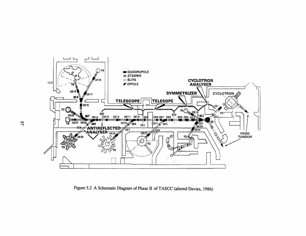
00 -..J
L_j L__j
• QUADRUPOLE a- STEERER + S.LITS ~DIPOLE
/
Figure 5.2 A Schematic Diagram of Phase II ofTASCC (altered Davies, 1986)

The survey for Phase liB was to be performed in August 1988 following the
reactivation of the beam line at the conclusion of the shut down period, which resulted in a
six month time differential between the surveys for the two subphases. The elements
involved in the Phase liB positioning are listed in Table 5.2 with Figure 5.2 illustrating
their locations with respect to the focussing doublet QE-11 (the completion of Phase llA).
The coordinating system ensembled at UNB (P3DCS) has been implemented in the
setting out of both subphases of Phase II of the TASCC accelerator. The UNB system
enabled the components of the accelerator to be positioned with the highest possible
achievable accuracies, while maintaining a real time interaction. This phase of T ASCC
involved the setting out of 7 bending magnets (dipoles), ranging in mass from a few to
almost 16 metric tons, and 60 much smaller focussing magnets (quadrupoles) to extend the
primary beam delivery system and create many additional experiment areas.
The main requirement in positioning accelerator components is maintaining a smooth
magnetic circuit throughout the entire length of the charged particle path (Gervaise, 1974).
The charged particle beam passing through the smooth magnetic circuit created by the
magnets or metal lenses is analogous to light rays passing through a series of glass lenses
in an optical system. Any misalignment of one of the glass lenses forming the system
creates a distorted image or possibly no image at all at the end of the system, but if all the
optical lenses were misaligned with respect to their design, yet still retained their relative
properties with each other a clear image would be formed. Carrying this over to the metal
lenses illustrates that it is not the absolute positioning of each magnet that is important, but
the relative accuracy between adjacent elements, especially those forming an operating unit
such as a quadrupole doublet or triplet.
The specifications for the alignment of the components comprising Phase II were
very stringent, requiring that the geometric centre of each element were positioned to no
worse than 0.1 mm in both transverse directions and 0.2 mm in the longitudinal direction.
Additional constraints to control the three possible rotations of each component have been
88

specified at no more than one minute of arc off the beam line design. Compounding the
specification requirements was the need to be able to determine the magnitude of
misalignment, in terms of the six degrees of freedom, in virtual real time to allow
adjustments to be made without any long computational delays. The ability to determine
corrections quickly in Phase IIA was imperative due to the time constraint imposed by the
time allotted for surveying activities in the shut down schedule. These restrictions were
made even more difficult by the realization that the extent of the portion of the accelerator
being installed covered a total length of over 40 m and has branch lines extending into four
additional enclosed experiment areas (see Figure 5.2).
The traditional methods of optical tooling involving the use of a horizontal alignment
telescope, horizontal spirit ("machinists") level with 10" per division sensitivity, and a
precision tilting level, were to be integrated with the more modern approach of the
coordinating system to satisfy completely the specification criteria listed above. The optical
tooling methods allow the magnitudes of the rotations to be determined by comparing
measurements of two targets defining the main axis of the element, while the coordinating
system can resolve the translations simply by determining coordinates of one of the main
axis targets.
5.2 The Establishing of the Reference Geodetic Micro-network
The establishing of the geodetic micro-network was required to satisfy the two
following conditions:
1. to create a reference for the design coordinates of the elements in the work area,
2. to facilitate locating the position of a theodolite, randomly set up in the work
area, with respect to the design coordinates of the elements.
Both conditions were a direct result of the use of the coordinating system for the project,
which applies three dimensional coordinate geometry to position theodolite stations and
89

object targets. If only traditional optical tooling methodologies were considered there would
be no need to create the micro-network, but the translation components of the misalignment
would be more difficult to obtain, especially in the longitudinal direction. Additional
benefits of creating the micro-network were to obtain a rigorous error estimation of target
locations, allow the placing of theodolites where "convenient", and to have a network of
reference points for future checking and maintenance surveys.
The micro-network established at CRNL consists of an array of targets adhered to the
concrete walls in both the main room housing the primary beam line and the experiment
rooms containing the branch lines. In the main room the targets have been installed at
approximately 2 m increments on the two walls parallelling the beam line, which are about
7 m apart, along the entire extent of the room. Figure 5.3 and Figure 5.4 give a plan view
of the target locations and the actual observation schemes in the main room and the
experiment rooms for Phase IIA and Phase liB, respectively. At each increment an attempt
to place two targets, at 3 m and 0.5 m above the floor, was made to guarantee a good
working range of values for the height components. The experiment rooms did not have as
stringent a control requirement as the main hall, therefore, for each room approximately 12
targets were placed around the experiment area at various heights. However, some
consideration had to be given for the placement of a few of the targets, to facilitate the
connection of the experiment and main rooms.
The targets themselves were the Wild adhesive type, which have a concentric circle
pattern that culminates in a 0.3 mm diameter solid dot at the centre. The concentric circle
target pattern was necessary due to the various oblique lines of sight that were used to
observe the targets and to facilitate the simultaneous horizontal and vertical paintings that
were performed. Brass plaques with a 5 mm thickness and having a surface area suitable to
adhere the adhesive target and a name tag, were manufactured at CRNL and installed on the
concrete walls at target locations.
90

\0 -
1460·11 R4eO-OJ
L••o-2• L410·0S
5 m. --·'
Control Survey Scheme as Observed
Figure 5.3 Observation Scheme for Phase IIA Control Survey (Secord et al. 1988)

\0 N
RM304-30 /
~~ /" ~
" ., W"'\ '
\ \ \ \~ \ \ \ \w .
li \ ~~.'~\'~~ I I .\--~ \~ \
I }-/;~y~\ \ \j_ \!. r; / /\\ \\\ l\'l.~ J/ // I I \\'X n';,\ J/ \\ \ '\ 1\t,"-
RM201-29 \\ \j ~\ \ ~ \ \\ .~ ,\\ \l\ b ,\ 1, r \, ~~ \ 1 \1 ~I \
~ ~ RM.21?·3.0
Control Survey Scheme
as Observed
0 .t:r==A
L~end
w.@ll lMJQPJ
~.Jw·
~fi\!,~.c:! .dlr:ecti.on and zenith angle
~
Sm.
Figure 5.4 Observation Scheme for Phase llB Control Survey

The definition of the datum for the network, as previously mentioned, was dependent
on the definition of the design coordinates of the elements to fulfill the conditions stated
above. All of the design coordinate values were with respect to the geometric centre of
dipole BE-l (labelled BE 1-C in Figure 5.5 and designating the end of Phase 1), which was
defined by a dowelled hole in its bottom yoke that could be made accessible for targetting.
Therefore, this becomes the logical choice for a fixed station that when the z axis is forced
to coincide with the local gravity vector, defines the origin of a horizontal plane at the
dictated beam line height (z coordinate) of 1.75260 m (69 inches) above the floor. An
existing target ("AXWEND") located at the very end of the main room gave the direction
for the designed horizontal path for the main delivery beam. This made that target very
suitable to be used to create orientation in the horizontal plane of the micro-network by
defining the x,z plane as the vertical plane passing through the geometric centre of BE-l
and the target AXWEND. The remaining y,z plane was defined as being perpendicular to
both the horizontal and x,z planes to create a right handed cartesian system. Figure 5.5
illustrates the relationship between the coordinate axes and the primary beam line.
Describing the coordinate axes in this fashion creates one irregularity concerning the
assumption of the gravity vector being straight and parallel throughout the CRNL facility.
This will obviously not be the case as the extent of the main beam line covers an area of
about 40 m in length. Neglecting this creates a maximum systematic deviation of 0.12 mm,
at the extrema of the main beam line, between a spatial line and the equipotential surface
defined by the level vials of the surveying instruments (see section 3.3.2). This deviation
systematically accumulates with progression along the beam line, but had no affect on the
relative smoothness between successive elements, which was the most important criteria
for consenting to the neglect of this effect.
The only remaining datum defect in the triangulation micro-network is the lack of
scale definition. The scale component was achieved by measuring directions and zenith
angles to the targetted ends of two calibrated scale bars, designed and manufactured at
93

\0 .J:>.
+ Y axis +Z axis I Beam Ht. above floor .
Figure 5.5 Datum Definition of the Control Network
T9
AXWEND 9 I I I I I I I I I I I I !

UNB, that had been situated in different locations throughout the network. The lengths of
the scale bars were treated as spatial distance observations with the targetted ends of the
scale bars (for each location) observed in the same ways as the wall targets, with their
coordinate triplets being estimated in the adjustment process. Each scale bar was
approximately 2 m in length and made from 6 mm invar rod with targets, the same design
as the Wild adhesive targets, attached to each end. The actual distance between a target pair
on a scale bar was measured to a standard deviation of± 0.01 mm, using an HeNe laser
interferometer, by the Laboratoire de Metrologie, Departement des Sciences Geodesiques et
Teledetection, Universite de Laval.
The error of± 0.01 mm involved in the calibration of the 2 m scale bars transformed
into a possible 5 parts per million (ppm) scale error in the coordinate determinations of the
micro-network. This error would have a systematic effect proportionally increasing with
distance away from the origin of the network (BE 1-C), reaching a maximum value of 0.2
mm for the x coordinates in the far end of the main room. However, similar to the effects
of the nonparallelity of the gravity vector, the relative accuracies between adjacent units
would remain very high. This allows the smoothness between elements to be maintained,
which again is the most important characteristic.
The observing of directions and zenith angles to the wall and scale bar targets was
facilitated by the UNB coordinating system, using the data gathering mode, which has been
described in section 4.3. This allowed data quality checks and station adjustments to be
performed, in real time, to determine beforing leaving a particular set up as to whether all
the data gathered was acceptable. The observing procedure and data quality checks used
have been fully described in section 4.2. The method of triangulation without sighting
between instrument stations, as described in section 3.4.3, was followed throughout the
measurements to achieve the highest possible quality of angular measurements.
95

Table 5.3 Statistical Summary of Phase llA Control Survey
Observables 591 Horizontal Directions (± 1 ") 591 Zenith Angles (± 1 ") 12 Spatial Distances(± 0.001 mm, artificial constraint*) 1 Azimuth(± 0.01 ",artificial constraint)
Unknown Parameters 477 Coordinates 51 Orientation (nuisance, associated with direction rounds)
667 Degrees of Freedom
The value 1.11 was estimated as the variance factor a posteriori and was found to be compatible at the 95% level of confidence with the value of 1.00 assumed a priori.
* The error of ±0.01 mm in the calibration of a scale bar has been considered as systematic and was not included in the error propagation of the adjustment.
Table 5.4 Statistical Summary of Phase liB Control Survey
Observables 245 Horizontal Directions (± 1 ") 245 Zenith Angles (± 1 ") 4 Spatial Distances(± 0.001 mm, artificial constraint*) 1 Azimuth(± 0.01 ",artificial constraint)
Unknown Parameters 201 Coordinates 17 Orientation (nuisance, associated with direction rounds)
277 Degrees of Freedom
The value 0.563 was estimated as the variance factor a posteriori and was found to be not compatible at the 95% level of confidence with the value of 1.00 assumed a priori, which showed the observations on average were more accurate than 1 arcsecond.
* The error of ±0.01 mm in the calibration of a scale bar has been considered as systematic and was not included in the error propagation of the adjustment.
96

All of the observations were combined to perform a single simultaneous least squares
adjustment to obtain estimates of the wall target triplets to be used in the setting out of the
elements and subsequently in their maintenance. The standard deviation of± 1" used for
the directions and zenith angles was computed while taking a pessimistic view of the a
priori error considerations discussed in section 2.2.2, to ensure that the propagated errors
of the wall targets were realistic. The estimated coordinate triplets of the theodolite stations,
scale bar targets, and orientation parameter for each round of observations are all
considered nuisance parameters and may be mathematically removed from the estimation
process if desired. A statistical summary for each of the two adjustments performed, Phase
IIA and Phase IIB, are contained in Table 5.3 and Table 5.4, respectively.
5.3 The Setting Out of the Components
The procedures used for the setting out of the accelerator components was identical
for both Phase IIA and Phase IIB. The coordinating system was integrated with traditional
metrological methodologies to create redundancy, while hastening the set out times. The
setting out can be broken down into targetting requirements, offset determinations, the
coarse alignment, the fme alignment, and future maintenance considerations. A discussion
of each of these topics is required to gain an understanding of how the project requirements
were met.
5.3.1 Targetting of the Component Axes
A very complex targetting problem was involved in defining the primary axis of the
quadrupoles to be positioned, which was the axis that had to be aligned with the designed
beam path. For a quadrupole this was an intangible axis and was defined as being the
geometric centre created by the 4 magnetic poles. Figure 5.6 shows the configuration of the
97
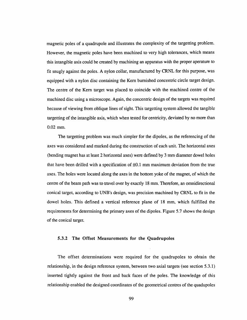
magnetic poles of a quadrupole and illustrates the complexity of the targetting problem.
However, the magnetic poles have been machined to very high tolerances, which means
this intangible axis could be created by machining an apparatus with the proper aperature to
fit snugly against the poles. A nylon collar, manufactured by CRNL for this purpose, was
equipped with a nylon disc containing the Kern burnished concentric circle target design.
The centre of the Kern target was placed to coincide with the machined centre of the
machined disc using a microscope. Again, the concentric design of the targets was required
because of viewing from oblique lines of sight. This targetting system allowed the tangible
targetting of the intangible axis, which when tested for centricity, deviated by no more than
0.02 mm.
The targetting problem was much simpler for the dipoles, as the referencing of the
axes was considered and marked during the construction of each unit. The horizontal axes
(bending magnet has at least 2 horizontal axes) were defmed by 3 mm diameter dowel holes
that have been drilled with a specification of ±0.1 mm maximum deviation from the true
axes. The holes were located along the axes in the bottom yoke of the magnet, of which the
centre of the beam path was to travel over by exactly 18 mm. Therefore, an omnidirectional
conical target, according to UNB's design, was precision machined by CRNL to fit in the
dowel holes. This defined a vertical reference plane of 18 mm, which fulfilled the
requirements for determining the primary axes of the dipoles. Figure 5.7 shows the design
of the conical target.
5.3.2 The Offset Measurements for the Quadrupoles
The offset determinations were required for the quadrupoles to obtain the
relationship, in the design reference system, between two axial targets (see section 5.3.1)
inserted tightly against the front and back faces of the poles. The knowledge of this
relationship enabled the designed coordinates of the geometrical centres of the quadupoles
99

to be transferred to either of the two targets located on the outside face of the poles, by
knowing the designed orientation of the quadrupole. However, this required the
assumption that the geometric centre of the quadrupole was actually the midpoint between
the two axial targets.
A quadrupole located on the main beam line had only one offset, which was in the
along beam direction (x axis of the control network). The amount of the offset was equal to
half the magnitude of the vector between the two axial targets inserted in either side of the
quadrupole. A quadrupole located on a branch line required that this offset value be
resolved into two orthogonal components, corresponding with the x andy axes of the
control network. The resolution into components was controlled by the angle that the
branch beam line made with the main beam line.
The determination of the magnitude of the vector was performed separately in a two
stage process. Firstly, by resecting two theodolites in the work area to the wall targets and
subsequently determining coordinates for the front axial target of a quadrupole by
intersections. Secondly, the theodolites were repositioned on the back side of the
quadrupole, where coordinates for the back axial target could be obtained by intersection,
without disturbing the quadrupole. Figure 5.8 illustrates all four theodolite locations
required to determine the offsets for a single quadrupole. Offsets for 5 or 6 quadrupoles
could be determined at one time, when the process was performed using a stable support so
the magnets would not move during the entire procedure. The magnitude of the vector
joining the geometric centre with one of the axial targets ranged between ± 0.2 mm, from
the overall mean value,..for all the quadrupoles with most being less than ± 0.1 mm.
In addition to the vector joining the axial targets, the coordinates to an
omnidirectional conical target, with the same design as that used for defining the dipole
axes, inserted in a dowel hole in the front top plate of the quadrupole (see Figure 5.6) were
determined. These coordinate values were reduced to offsets with respect to the geometric
100

o Theodolite Station
11 Wan Targc~
.,/
~ /
' /
' / ' /
' / ' / ' / ' ' ' / ~
/
' / ' /, ' ' /' ~
/
' ,_. ' ,_. ' /
' /
' ,/ ,"\ ,, ' ,_. i"'·., ;',. 1' ... ' / ' ,_. ' / ., ' ' ' ./ ' ' ' ,/ ' / ' , ' , ' , ' ' ' , ·,_. ' ' , ' , ' ,/ ' ./ ' / ·' ' , t·_, ' ' /
' , ' , ' , ' /
' / ' ' ' /
' /
' , ' '
Figure 5.8 The<Xiolite Locations for Quadrupole Offset Determinations
101

centre of the quadrupole, which will be used in the future maintenance of the TASCC
system (see section 5.3.5).
5.3.3 The Coarse Alignment
When the magnets were positioned to within the specifications of their nominal
locations the quadrupoles were supported on stands and the dipoles on concrete pedestals.
This implies that a coarse alignment had to be performed, which simply involved setting
out of the supports to within the working range of the fine adjustment mechanisms (± 5
mm), for both the quadrupoles and the dipoles.
The quadrupole support stands were manufactured in the CRNL shops from special
pressure treated steel to ensure that no load deformation in the location of the positioned
elements would occur, once in place. The stands themselves were scribed in the machine
shop with reference lines enabling them to be properly oriented and set to within the
specified distance along the beam line very easily. The procedure simply involved an
alignment telescope for horizontal orientation, tilting level for the vertical orientation, and a
steel tape for the distance along the beam line. Once aligned, the stands were bolted to the
floor, their alignment rechecked, and if found satisfactory they were grouted in place for
stability.
The dipoles required concrete pedestals for stability due to their enormous bulk and
critical locations (the bending points of the beam line). The coarse alignment consisted of
positioning the forms for the poured concrete and the anchor bolts, for securing the tubular
steel support base for the dipole. A steel plate, the same shape as the pedestal, was scribed
with lines representing the beam axes and had holes drilled in it describing the required bolt
pattern with respect to the beam axes. The plate was aligned with respect to the designed
location of the beam axes, which gave the positions of the pedestals and the appropriate
102

bolt pattern orientation. This portion of the coarse alignment was considered part of the
construction and was performed by CRNL with their own staff on site.
5.3.4 The Fine Alignment
The fine adjustment was very similar for both the quadrupoles and dipoles,
incorporating an iterative procedure to converge to within the specifications for their
nominal locations. The instrumentation used for the traditional metrology procedures
employed a Kern DKM2-A single second optical mechanical theodolite with a parallel plate
micrometer, a Wild N3 precision tilting level, and a machinist's horizontal spirit level with
10"/division sensitivity. As previously described, the coordinating system was comprised
of two Kern E2 electronic theodolites interfaced to a Macintosh Plus microcomputer.
For the coordinating system, the electronic theodolites were located around the
element to be set out in a way that optimized the intersection geometry and created average
sight distances of approximately 5 metres. A typical instrument set up showing the
redundant resections and the locations of the electronic theodolites with respect to the
element is shown in Figure 5.9. Two sets of direction measurements to 8 to 10 control
targets were performed for each resection, in an attempt to randomize the effects of the
control target errors.
For the traditional methods, the DKM2-A was used as a horizontal alignment
telescope, which required it to be located in the vertical x,z plane defined by the designed
beam line. For the main beam line, this was accomplished using an iterative measurement
of the included angle (near 180 degrees) procedure (Chrzanowski, 1983). This method
could be utilized because of the accessibility of the end targets at BE1-C and AXWEND,
which defined the extremes of the beam line as well as the datum for the control network
(see section 5.2). For the branch lines, the beam line was defined by the targets inserted in
the dowel holes that were located in the bottom yoke of the relevant dipole, that had already
103

l :Quadrupole on'
~:.....-__ _,! the stand
o Theodolite Station 11 WallTargen
Figure 5.8 Typical Theodolite Locations for the Setting Out Survey
104

been set out on the main line. Therefore, the DKM2-A had to be brought on line by an
iterative extrapolation of the direction given by the inserted targets.
For both the dipoles and quadrupoles, the design of the fine adjustment mechanisms
were conducive to allowing the horizontal and vertical adjustments to be segregated in the
setting out procedures. The four vertical adjustment bolts (a ball and cup assembly) for a
quadrupole, were located in the centre of each side of the base plate. The bolts were
machined with a ball at one end, which fit into a cup that was fastened securely to the
quadrupole stand. The quadrupole could be raised or lowered, rotated around the beam
line, and rotated along the beam line, simply by threading the appropriate bolts in/out of the
base plate. The five horizontal adjustments were located beside the vertical bolts for the
front and both sides, while the back contained two horizontal adjustment screws located
outwardly towards the sides of the base plate. The horizontal adjustment mechanism is the
same as that for the vertical, except that the screws are threaded through a block of metal
that has been fixed to the top of the base plate into cups that are no longer stationary, but
push against the quadrupole. The remaining three degrees of freedom could be adjusted by
backing off the adjustments on one side while tightening the appropriate ones on the
opposite side.
For the dipoles, the tubular supports securely bolted to the pedestals contained all of
the adjustment mechanisms for adjusting them. The dipole itself rested on three small brass
plaques, whose heights could be controlled by large diameter finely threaded bolts,
machined with a ball on one end, that were attached to the tubular supports. The dipole
could be raised or lowered, rotated around the beam line, and rotated along the beam line,
simply by threading the appropriate bolts in/out of the tubular support. Two square
brackets, located on either end of the support, were used for the horizontal adjustments.
Each bracket contained four screws that were positioned perpendicular to each other in the
horizontal plane, which were oriented to allow movement in the transverse and longitudinal
incoming beam line directions. The remaining three degrees of freedom could easily be
106

removed by pushing the screws against metal blocks that were securely fastened to the
dipole and fit into the square brackets.
Each quadrupole was guided into its nominal location by integrating the traditional
optical tooling methods with the coordinating system and following the procedure listed
below.
1. Removal of rotation about the beam axis (x axis) by the horizontal machinist's
(spirit) level placed on the forward horizontal top plate of the quadrupole (see
Figure 5.6). A special adaptor and rotatable mirror assembly was designed by
UNB to allow the placing of the level on the front plate and to facilitate the viewing
of the vial.
2. Removal of the forward/backward rotation (y axis) by sighting the two axis
targets using the Wild N3 (reference plane is created by initially sighting a
conical target inserted in a dowel hole of an already set out dipole).
3. Removal of the z translation by paired intersections to one of the axis targets
from the two resected Kern E2 theodolites.
Steps 1, 2, and 3 were repeated until all three discrepancies were eliminated.
4. Removal of the along beam line translation, which is along the x axis on the
main beam line, by paired intersections to one of the axis targets from the two
resected E2 theodolites, with the required offsets applied (see section 5.3.2).
5. Removal of the rotation about the z axis through horizontal transverse alignment
using the Kern DKM2-A, which has been brought on line using one of the
appropriate methods, as discussed above.
6. Removal of the translation transverse to the beam line, which is the y translation
on the main beam line, by paired intersections to one of the axis targets from
the two resected E2 theodolites. The branch lines required an offset to be applied
to remove they translation(see section 5.3.2).
107

Steps 4, 5, and 6 affect the results of steps 1, 2, and 3. Hence, all six steps were repeated
until all six discrepancies were negligible.
For the setting out of the dipoles, steps 1, 2, and 3 above can be replaced with the
following:
1.& 2. Removal of the rotation about the beam axis (x axis) and along the beam axis
(y axis) by the horizontal spirit level positioned on the bottom yoke, to use the
three height adjustment screws in the same fashion as leveling the vial of a
theodolite.
3. Removal of z translation by paired intersections to an omnidirectional
conical target placed in an on axis dowel hole on the bottom yoke.
A final set of intersections were made to the axis targets and derived discrepancies
were compared with those obtained from the optical tooling instrumentation. Excessive
differences were investigated until they could be resolved. Any further adjustments led to
additional intersections until all discrepancies and differences were negligible.
The coordinating system itself was capable of determining the coordinate triplets of
the axial targets, however, the Wild N3 and Kern DKM2-A provided redundancy for the z
andy translations respectively, ensuring reliable results. Appendix I contains the computed
discrepancies between the designed coordinates and those determined by the coordinating
system in the setting out, for both Phase IIA and Phase liB. Figure 5.11 illustrates a
portion of the already aligned beam line after all of the hardware has been installed.
5.3.5 The ·Maintenance of the System
Once the TASCC accelerator components had been positioned to their nominal
locations, a system had to be devised to permit the checking and relocating of the element
positions in the future. The poles forming both the quadrupoles and dipoles will no longer
be accessible for targetting once the beam line is commissioned, primarily due to the
108
insertion of vacuum tubes that are required for the beam. In addition, the centre element of
a quadrupole triplet has both its axial targets blocked from view, for the oblique lines of
sight required by the coordinating system, by the two remaining members of the triplet.
The inaccessibility problem could be overcome by placing accessible targets on the
side walls of each individual element and determining their vector relationship with respect
to the element's geometric centre. For a quadrupole, two Wild self adhesive targets were
adhered to opposite sides of the frame (see Figure 5.6), to create as long a baseline as could
be observed using the coordinating system. The targets, called "wing targets", were tied to
the reference control network using triangulation, which gave their position with respect to
the already set out position of the element (see section 5.3.4). The same procedure was
used for a dipole with a third adhesive target replacing the conical target. The "wing
targets" combined with the vertical offset of the conical target previously determined, can
be used to eliminate all the degrees of freedom involved in the repositioning of an element.
The "wing targets" combined with the array of wall targets forms the maintenance
system that can be used to check and reposition any element in the TASCC system in the
future. However, as the setting out was done using coordinate determinations the
maintenance scheme itself is centered around being able to redetermine the "wing target"
values. This could be a very time consuming process for a routine inspection of all the
elements or if a group of elements are suspect to deformation.
The placement of the "wing targets" on the quadrupoles was done with particular
attention being taken to ensure that the targets were located at the same height on each
element, at least within the· working range of aprecision level's micrometer (10 mm). This
enables a quick relative check to be performed, independent of the wall targets, utilizing the
height differences between the "wing targets" determined initially. In addition, during the
setting out procedure, the front top plate of each quadrupole was levelled, in the direction
transverse to the beam line, using a precision machinist's level. This creates another
109

independent check as to whether an element has moved nonuniformly in the vertical,
simply by monitoring the amount of mislevelment of this plate.
If the position of an element is to change, it is highly unlikely that it would occur in
only the horizontal location without affecting the vertical component. Therefore, the above
independent checks can be relied on very heavily to detect or confirm any changes that may
be occurring in element positions. However, because the quick check methods rely solely
on vertical changes, they are limited to being able to detect movements and cannot be used
by themselves for readjusting an element. The use of the coordinating system is the only
recourse for repositioning an element once it has been detected as being unstable or is being
reinstated after repairs. The quick checks can be used to provide a degree of redundancy for
the vertical in the repositioning.
5.4 The Stability of the Micro-Network
The stability of the micro-network for both the short and long terms is very
important. The short term stability was imperative to maintain the same reference datum for
all of the setting out procedures ensuring that the relative smoothness of the entire system is
maintained. The long term stability is required to allow future monitoring of the element
positions as well as removal and reinstallation without sacrificing any of the relative
smoothness obtained in the initial installation.
The main frame of the portion of the building housing the TASCC accelerator was
constructed in the 1940's. Canadian specifications for nuclear facilities are very stringent
requiring very thick poured concrete walls and floors, with reinforcing steel and without
dilatation gaps. This creates a very sound structure with some of the interior and exterior
walls approaching a thickness of 4 feet, and such are the walls where the targets forming
the micro-network have been installed.
110

The expectation was that the short term stability would be guaranteed due to the
enormous bulk of the structure. However, an attempt to improve wall target triplets and
enhance their accuracies by combining network and set out observations, carried out over a
time span of a month, into a single simultaneous adjustment for Phase IIA results in
discrepancies between estimated results from the initial and combined adjustments. The
discrepancies, contained in Appendix II, show a systematic decrease with accumulated
distance from the origin for the two horizontal coordinates for each target. The changes are
up to a maximum of 0.32 and 0.06 mrn for the x andy axes respectively, which transforms
into a suggested scale change of -7 ppm.
The scale bars themselves were only introduced to determine scale during the original
network survey, therefore, any scale error contribution by them could not possibly be seen
in the results of the combined adjustment. Assuming the above discrepancies are scale
related and elimination of the scale bars as the reason, leaves the only other possibility that
the wall targets themselves have moved. The systematic contraction of an entire wall to
duplicate a scale change points to the suspicion of the walls being affected by thermal
expansion, which is further substantiated because no dilatation gaps exist.
The coefficient of thermal expansion for concrete is given as lxl0-5/co which
means to create a -7 ppm scale change the walls would only have to undergo an average
change in temperature of -0.7 co. During the setting out survey, which was performed
during the on going construction, the outside and inside temperatures differed by lO's of
C0 resulting in large temperature fluctuations when construction materials were brought
inside, by opening the entrance from outside. On numerous occasions the setting out had to
be halted to allow the temperature to stabilize as it affected both instrumentation
(compensators in theodolites) and lines of sight (refraction). The long term effect on the
concrete walls of these short term temperature fluctuations is difficult to determine, but
clearly with such large temperature differences the effect cannot be considered negligible.
The long term effects of the continually large outside and inside temperature differential will
111

Table 5.5 Displac.ements and Error Ellipses (95%) fDJ' XY PlaJ'U~
Station Dx Dy TotalDisp AzofDisp a b AzQfa To Ellipse Periphery (mm) (mm) (mm) llkg.} (mm) (mm) (d~g;~ (mm)
L220-28 -.20 .17 .26 310.6347 .36 .t9 29.6,.$96.3 .34 * L240-28 -.10 .19 .22 332.1854 .32 .17 29:8.2210 .24 * L266-28 -.09 .22 .23 338.4848 .28 .12 3n6..238:8 .19 ** L280-28 -.05 .14 .15 339.4244 .25 .11 3,('1:8.,.8,('13 7 .18 * L300-28 -.02 .04 .04 332.4126 .22 .11 31~9 • .0.1'1'99 .20 L320-28 .03 .04 .05 31.0427 .21 .10 33J.4BH .11 * L340-28 .03 .06 .07 27 . .8510 .20 .08 34.3.3'5.:$1 .11 * L360-28 .00 -.02 .02 171.3245 .21 .08 3SR.6J:l5S .20 L381-28 .02 -.10 .11 170.1925 .21 .09 16$14:.8 .15 * L400-28 -.03 -.11 .12 195.4373 .22 .to 3.0c.OiH:§. .19 * L420-28 .06 -.13 .14 15.6.0500 .25 .11 42$8.9<8 .12 **
>-' L440-28 .05 -.13 .14 15.8.9996 .28 .12 51.7~0112 .13 ** >-' N L460-28 .05 -.01 .05 98.7221 .33 .14 57.174;5 .19
R240-28 -.20 .00 .20 270 .. 8940 .27 .07 87 .. 929,() .27 * R260-28 -.14 -.12 .19 228.8983 .23 .09 84,4Tl9 .14 ** R260-03 -.13 -.01 .13 2.6,6.8372 .24 .0:8 8:t~l63.5 .24 * R272-28 -.10 -.13 .17 218.0738 .21 .09 84.169:8 .11 ** R300-28 -.07 -.19 .20 199.7154 .17 .09 71.84~l0 .11 ** R300-03 -.04 -.06 .07 212.3871 .1 7 .11 73.147:2 .13 * R320-28 .00 -.20 .20 180.9340 .14 .09 3,8,.3,(),84 .12 ** R343-28 -.04 -.09 .10 202.6107 .18 .08 8.45.Cl8 .16 * R343-03 .05 -.07 .09 144.4088 .18 .08 8A3Al:5 .11 * R360-28 .01 -.05 .05 16.6.9789 .17 .08 354. 7:_474~ .16 R380-03 .11 .02 .11 78.3442 .17 .09 342.fl52:3 .09 ** R395-30 -.04 .05 .06 322.8777 .18 .10 32.6.,£),_(1)!1:3 .18 R410-30 .03 .05 .06 29.8312 .18 .10 3.03,.8A60 .10 * R422-03 .07 .01 .07 85 . .9098 .19 .10 28:8.,6139 .17 * R422-28 .01 .05 .05 15.8400 .20 .11 2:9;1,0,3:54 .11 * R440-28 .04 .08 .09 22.8851 .24 .12 2:8:5 •• :8A.Z.4 .12 * R460-28 .02 .08 .08 11.7912 .30 .13 2:83.126.3 .13 * R460-03 .06 .00 .06 89.2711 .30 .06 2.7~8.,89--44 .24

Table 5.6 Displacements and Error Ellipses (95%) for XZ Plane
Station Dx Dz Total Disp AzofDisp a b Azofa To Ellipse Periphery (nun) (mm) (mm) (~~~g.) (mm) !,mmj (de g) (mm)
L220-28 -.20 .01 .2·0- 272.5277 .33 .07 273:--f297 ~33' * L240-28 -.10 .01 .10 274.2765 .29 .0.6 27'2 .. 7677 .29 L266-28 -.09, .00 .09 2.69.0327 .24 .04 274 .. 5.027 .20 * L280-28 -.05 -.08 .09 214.8248 .21 .06 27·.6.375.6 .07 ** L300-28 -.02 -.10 .10 192.2721 .17 .06 276.2105 .06 ** L320-28 .03 -.09 .09 163 .. 8.526 .13 .0.6 2.81 . .23l0 .07 ** L340-28 .03 -.06 .07 153.452.6 .10 .06 2:87.5tl15 .07 * L360-28 .00 -.03 .03 174.1309 .08 .06 297.1403 .06 * L381-28 .02 -.02 .03 135.5.085 .10 .06 2:7·0.2117 .07 L400-28 -.03 .05 .06 327.9714 .14 .07 87.237-5 .08 * L420-28 .06 .11 .12 27.2908 .19 .0:8 8.5.4002 .09 **
..... L440-28 .05 .12 .13 21 . .9207 .24 .08 86 .. 1432 .09 ** ..... L460-28 .05 .18 .19 -16.1323 .29 .09 84. •. 8182 .10 ** w R240-28 -.20 .09 .22 294.3081 .27 .07 276~l9.K8 .18 ** R260-28 -.14 .10 .17 306.7311 .23 .07 27 5~5,6.8.6 .12 ** R260-03 -.13 .00 .13 2.69.2616 .24 .03 8.3 •. 6.6.8-9 .19 * R272-28 -.10 .13 .17 321.0372 .21 .07 274.2:8:3.1 .09 ** R300-28 -.07 .16 .17 336.9482 .16 .0.6 27$.9i8.Ql .07 ** R300-03 -.04 .02 .04 295.,6190 .17 .06 77.71l0 .09 * R320-28 .00 .23 .23 359.18.6.0 .12 .0.6 27•9,7472 .06 ** R343-28 -.04 -.01 .04 252.48.09 .0.8 .07 2:7~8 .. .92.65 .08 * R343-03 .05 -.14 .15 159.4006 .10 . .07 3,6..0527 .08 ** R360-28 .01 -.04 .05 165.0424 .08 .06 71.132:1 .06 * R380-03 .11 -.10 .15 132 . .2967 .11 .0.8 3.10 .. ,5,613 .11 ** R395-30 -.04 -.10 .11 199..58.62 .13 .06 81.18,02 .07 ** R410-30 .03 -.06 .06 153.35.6.6 .16 .05 8:5,.$805 .0.6 ** R422-03 .07 -.06 .09 127.5564 .20 .0'8 2'8;8.272.6 .16 * R422-28 .01 -.02 .02 141.29.09 .19 .05 8;8,,657'9 .07 R440-28 .04 .00 .04 83.374.8 .24 .03 8:8 .. 9>9.6.9 .20 R460-28 .02 .10 .10 9.2210 .3.0 .07 87.7'58.5 .07 ** R460-03 .06 .04 .07 5.6.4980 .31 .07 2.8.5.5449 .09 *

Table 5.7 Displacements and Error Ellipses (95%) for YZ Plane
Station Dy Dz Total Disp AzofDisp a b Azofa To EUips.e Periphery (mm) (mm) (~11!) (de_g.) (mm) (mm) (cJ_e_~} (m~)
L220-28 .17 :or· .17 87.0552 -~24~ :o.6~ 81.5.81.0 .22 * L240-28 .19. .01 .19 87.740.8 .22 .05 81.4741 .20 * L266-28 .22 .. .00 .22 9.0. • .3.813 .19 .04 84 .. 6.648 .17 ** L280-28 .14 -.08 .16 118 . ..3520 .18 .0.6 8.0 .. 8:877 .09 ** L300-28 .04. -.10 .10 157 .. 3974 .18 .0.6 82.55.69 .06 ** L320-28 .04 -.09 .10 154 .. 3102 .19 .0.6 82 .. 7692 .06 ** L340-28 .06 -.0.6 .0.8 1.3.6.6028 .19 .06 8.3Jl202 .07 ** L360-28 -.02 -.03 .04 213.96718 .21 .0.6 81.743,0 .0.8 "' L381-28 -.10 -.02 .11 2.60..0203 .20 .0.6 8.2 . .842.9 .20 * L400-28 -.11 .05 .12 2~93 ... 8184 .20 .0.6 8.0 ... 6.18;5 .10 ** L420-28 -.13 .11 .17 310.7261 .20 .07 7'7,$8.6.6 .08 ** L440-28 -.13 .12 .18 313,.,6488 .20 .07 78 .. 8.976 .09 ** -- L460-28 -.01 .18 .18 3.5'!1.4592 .22 .0.8 . 77.1-679 .09 ** ~
R240-28 .00 .09 .09 1.9787 .08 .07 327.4;2:96 .0.8 ** R260-28 -.12 .10 .16 31.0.5423 .10 .0.6 29·9.948.2 .10 ** R260-03 -.01 .00 .01 256 .. 8704 .09 .03 74.0.6.69 .09 R272-28 -.13 .13 .18 314.087'8 .10 .06 297"6023 .09 ** R300-28 -.19 .16 .24 310.1013 .11 .0.6 28.6~.6.1 02 .09 ** R300-03 -.06 .02 .0.6 2K6.9l80 .12 .0.6 ~0.8.029 .09 * R320-28 -.20 .23 .31 318 .. 92.66 .13 .0.6 2:84.55.69 .08 ** R343-28 -.09 -.01 .09 2.62 .. .5104 .18 .0.6 2~80.2.0.00 .14 * R343-03 -.07 -.14 .15 207.7-071 .19 .07 70..0523 .10 ** R360-28 -.05 -.04 .07 22·9.1199 .17 .0.6 27~~.551-4 .07 * R380-03 .02 -.10 .1.0 167.225.3 .17 . .07 67 ... 54.62 .08 ** R395-30 .05 -.10 .11 154 .. 8.222 .16 .0.6 27'9. .. 65.68 .07 ** R410-30 .05 -.06 .0;8 138 .. 8164 .13 .05 '2/'1'7.,8:847 .07 ** R422-03 .01 -.0.6 .06 174 .. 68.6.6 .13 .07 5.4 •. &932 .08 * R422-28 .05 -.02 .05 109.495.6 .12 .05 277.1114 .11 * R440-28 .08 .00 .08 87.1932 .13 .03 2"1'6.()5.60 .11 * R460-28 .08 .10 .13 37,8714 .14 .06 2:82.7'947 .07 ** R460-03 .00 .04 .04 1.1011 .12 .05 3.0.920.8 .08 *

certainly create some thermal expansion in the outside walls, which form part of the
reference network.
It is the above findings that became the criteria in deciding to resurvey a portion of
the main micro-network, described in section 5.2, thatwould be involved in the Phase ITB
setting out. A by-product of this completely independent survey is the ability to determine
the displacement vector for each target between the two epochs of survey. The
displacements are determined with rigorous error estimations by removing the datum biases
created by the adjustment minimal constraints, using the weighted projection methodology
(iterative weighted s-transformation), which is part of the generalized approach developed
at UNB for modelling deformations (Chrzanowski et al. 1982; Chen, 1983; Secord, 1985;
Chrzanowski, 1986). The displacements for the targets involved are projected onto the
three coordinate planes with Tables 5.5, 5.6, and 5.7 giving the components with error
ellipses for the (x,y), (x,z), and (y,z) planes, respectively. The figures contained in
Appendix Ill illustrate the magnitudes of the projected displacements with respect to their
corresponding 95% confidence level error ellipses in the (x,y), (x,z), and (y,z) planes,
respectively. The projected displacements for the (y,z) plane are illustrated in a series of
cross sections, for reasons of clarity, because their projected locations are almost identical
in this plane.
It can be clearly seen from the illustrations that even over just a 6 month period the
movement of some of the targets is significant (up to 0.31 mm in the y,z plane) and there
are some systematic trends to the changes. This unfortunately poses some serious doubts
on the ability of the micro-network to remain stable in the long term. However, if the
displacements detected here have been temperature induced then rigorous environmental
controls may be the answer to the longevity of the micro-network.
Continuing on this line, the setting out survey for Phase llB had a similar time span
as that for Phase IIA. However, the inside temperature was kept constant at 17 oc
throughout, with the magnitude of the inside outside temperature differential only a few
115

degrees for the entire setting out. In addition, this same temperature differential had been
occurring at least two months previous to the Phase liB setting out survey. The same
procedure of combining the set out observations with the repeated network observations
and performing a simultaneous adjustment was repeated for Phase llB. The result was that
the original expectation was achieved, namely, improved target triplets with only slight
changes in values between adjustments. This result further substantiates the theory of long
term thermal expansion of the concrete walls and gives a little more credibility to
environmental controls.
116


6. Conclusions and Recommendations
The objective of this thesis was to give some insight and lift some of the mystique
surrounding the new technology of coordinating systems for use in industrial metrology.
To accomplish this, discussions were required describing the working components of the
systems, primarily the theodolites. With interfacing to a microcomputer and using the well
established geodetic surveying procedures, accuracies of a few hundredths of a mm are
possible over short distances. An additional objective was to show that traditional optical
tooling methods should not be replaced by coordinating systems, but the two should
complement each other and they should be integrated to allow optimum accuracies to be
achieved, with strong reliabilities, and minimal observational effort. Each methodology has
assets over its counterpart that cannot be taken away.
The comparison of electronic theodolites with their optical-mechanical versions
showed conclusively that the circle reading and automation of data collection are the only
differences between the two. The newer electronic instruments still require the same basic
solid mechanical structure, and once given this, are capable of achieving angular
measurements with an expected accuracy improvement of a factor of 3 over their 1" optical
predecessors mainly due to the improved accuracy of the electronic circle reading. In
addition, electronic instruments with biaxial compensators are able to maintain this
improvement, both horizontally and vertically, for long durations of time. Instruments
equipped with uniaxial compensators allow the instruments to be levelled very precisely
initially, but have no way of correcting the horizontal circle readings for level drift during
use. Stability of instrument set ups over long periods of time are the norm in industrial
metrology, which means an electronic theodolite with a biaxial compensator must be made
117

the standard instrument in coordinating systems, to maintain reliability throughout an
observing session.
The accurate determination of network scale has been a problem facing geodesists
since the beginning of triangulation and now for the confmed areas of industrial metrology
seems to be the limiting factor as well. The maximum length of a precisely calibrated scale
bar, due to the logistics of calibration and transportation, is 2 to 3 m. If the bar can only be
calibrated to± 0.01 mm this results in a 3 to 5 ppm systematic scale error in the project
area. If it is a small confmed project, like the antenna experiment, then this isn't a problem,
however , the TASCC project covered over 40 m which introduced a maximum systematic
error of up to 0.2 mm in that direction! Fortunately, for this project the systematic scale
error was not a major concern, but it does illustrate the problems associated with the
determination of network scale that must be overcome to advance the capabilities of the
coordinating systems.
The traditional methods of triangulation prove to be reliable for the establishing of
geodetic micro-networks. The merit in the incorporation of the unique method of
triangulation with the "free positioned" theodolites without sighting between theodolite
stations, to increase angular accuracy, has been displayed by the adjustment results of
TASCC Phase liB, where the internal room temperature was kept constant. If the a
posteriori variance factor (0.56) is used to scale the observation variance-covariance matrix
then the expected accuracies discussed in section 2.2 for the Kern E2 are obtained.
The stability of geodetic micro-networks is critical in industrial applications where
measurements are performed periodically to check alignment, calibrate a robotic arm, or
determine the shape of an assembled surface. Based on the results from TASCC, it can be
appreciated that the influences of long term thermal expansion could easily produce biased
results at the level of accuracy usually sought in these applications. In addition, the bulk of
the effect is due to inside outside temperature differentials, which are not easily removed or
modelled. Inside environmental controls can be implemented, as was the case at T ASCC,
118
but they will only help the observing consistency and will do very little for long term
thermal expansion, due to the inside outside temperature differential.
The observation reductions for the effects of gravity, in most cases, may be ignored
due to the small areas of interest creating negligible changes in the deflections of the vertical
and direction of the gravity vector. However, there may be instances where nonparallelity
of the gravity vector throughout the project area may have to be considered to achieve
results at the few hundredths of a mm level. Again, the T ASCC project illustrates this by
showing the possible maximum deviation of 0.12 mm between a spacial line and an
equipotential surface.
The algorithms developed in chapter 4 have been implemented with great success in
the TASCC project. The data used in the least squares adjustments, for both Phase IIA and
B, to determine the micro-network target triplets combined together very favorably as
shown by the statistical testing summaries contained in section 5.2. Observational
blunders, mispointings, and electronic glitches had all been removed or reobserved during
the data acquisition process using the data quality check algorithm. A visual inspection of
the collimation error, index error, and discrepancies between the observed set of angular
quantities and their mean values is procedure enough to ensure that only data of adequate
quality is maintained and used in coordinate determinations. The data checks are imperative
when locating theodolites in the work area, where the observations are used in real time to
obtain theodolite station as well as object target triplets. However, collimation and index
errors are obtained to be analysed only if observations are performed in both positions of
the theodolite telescope, which is a requirement for coordinating systems as shown by the
discussions in sections 2.2 and 3.4. All errors inherent in theodolite construction, with the
exception of vertical axis error, may be removed by observing a direction in both positions
of the telescope. Manufacturers attempt to eliminate the errors as best they can during the
assembling of the components, but not all errors behave consistently (i.e. collimation and
index errors) as shown in section 2.2.
119

The least square adjustment algorithms made it possible to obtain the theodolite
station triplets by redundant resections. This enabled a number of wall targets to be
observed for each theodolite set up, randomizing their effects on the overall result and
creating very well defined theodolite locations. The same algorithms also made it possible
to relocate each theodolite independently in the work area which created a great deal of
flexibility and allowed some time to be saved in the setting out process.
The TASCC project has proven to be a very adequate environment for testing the
practicability of the developed algorithms, establishing micro-network methodology, and
integrating traditional optical tooling with a coordinating system. An indication of the
quality of the alignment results can be obtained with the realization that, for Phase llA, only
a few hours were required to commission the beam at the conclusion of the construction.
Unfortunately, results for Phase Iffi are not yet available as the supporting hardware (i.e.
vacuum tubes, beam line monitors, slit assemblies, etc.) is still being installed.
120

References
Ackerson, D. Scott. "Uses of WILD C.A.T. 2000 Electronic Theodolites with Robots and Robot Workcells." Paper commissioned by Wild Heerbrugg Instruments, Inc., Farmingdale, New York, 9 pp.
Bauke, Walter E. (1983). "Adaption of Precision Surveying for Alignment of the Antares Laser Inertial Fusion System." The Proceedings of the American Congress of Surveying and MaP.Ping. Annual Meeting, Washington D.C., Mar., pp 676-685.
Bauke, Walter, David A. Clark, Peter B. Trujillo (1985). "Surveying and Optical Tooling Technologies Combined to Align a Skewed Beam Line at the Lampf Accelerator." The Proceedings of the American Congress of Surveying and Mapping. Annual Meeting, Washington D.C., Mar., pp 311-320.
Bethel, James, John Sedej (1986). "Submarine Hull Mapping and Fixture Set-Out: An Application of the ECDS System." The Proceedings of the American Congress of Surveying and Mapping. Annual Meeting, Washington D.C., Mar., pp 92-96.
Blachut, T. J., A. Chrzanowski, J. H. Saastamoinen (1979). Urban Surveying and Mapping. Springer-Verlag New York Inc., New York, USA, 372 pp.
Bomford, G. (1980). Geodesy. 4th Edition, Oxford University Press, 855 pp.
Brown, Duane C. (1985). "Adaptation of the Bundle Method for Triangulation of Observations Made by Digital Theodolites." Proceedings of the Conference of South African Surveyors, Paper No. 43, 18 pp.
Campbell, Joe (1984). The RS-232 Solution. SYBEX Computer Books, Berkeley, Ca, USA, 194 pp.
Chen, Yong-qi (1983). Analysis of Deformation Surveys- A Generalized Method, Dept. of Surveying Engineering Technical Report 94, University of New Brunswick, Fredericton, N.B., Canada, 262 pp.
Chen, Y.Q., M. Kavouras, A. Chrzanowski (1987). "A Strategy For Detection of Outlying Observations in Measurements of High Precision." The Canadian Surveyor, Vol. 41, No.4, winter, pp 529-540.
Chrzanowski, A. (1977). Design and Error Analysis of Surveying Projects, Dept. of Surveying Engineering Lecture Notes 47, University of New Brunswick, Fredericton, N.B., Canada, ??? pp.
121

Chrzanowski, A., Y.Q. Chen, J.M. Secord (1982). "On the Analysis of Deformation Surveys." Proceedings of the 4th Canadian Symposium on Mining Surveying and Deformation Measurements, Banff, Alberta, June, pp 431-452.
Chrzanowski, A. (1983). Selected Topics in Engineering Surveys Part III- Alignment Surveys, Dept. of Surveying Engineering draft lecture notes and supplementary reading material, University of New Brunswick, Fredericton, N.B., Canada, 153 pp.
Chrzanowski, A. (1985). "Implementation of Trigonometric Height Traversing in Geodetic Levelling of High Precision." Contract Report. 85-006, Geodetic Survey of Canada, 93 pp.
Chrzanowski, A., Y.Q. Chen, J.M. Secord (1986). "Geometrical Analysis of Deformation Surveys." Proceedings of the Deformation Measurements Workshop. Modem Methodology in Precise Engineering and Deformation Surveys-II, Massachusettes Institute of Technology, October, pp 170-206.
Cooper, M.A.R. (1982). Modem Theodolites and Levels. Granada Publishing Ltd, London, 258 pp.
Curtis, C., W. Oren, R. Ruland (1986). "The Use of Intersecting Lasers in the Alignment of the New Electron-Positron Collider at the Stanford Linear Accelerator Center." The Proceedings of the American Congress of Surveying and Mapping, Annual Meeting, Washington D.C., Mar., pp 61-69.
Davies, W. G. (1986). "Design of the Extraction Beam Lines for the Chalk River Superconducting Cyclotron." The Proceedings of the XI International Conference on Cyclotrons and their Applications, Tokyo, Japan, Oct. 13-17.
. . . Deumlich, Fritz (1982). Surveying Instruments. Walter de Gruyter, Berlin I New York,
316 pp.
Faig, Wolfgang (1972). Advanced Surveying I, Dept. of Surveying Engineering Lecture Notes 26, University of New Brunswick, Fredericton, N.B., Canada, 225 pp.
Friedsam, H., W. Oren, M. Pietryka, R. Pitthan, R. Ruland (1985). "The Alignment of Stanford's New Electron-Positron Collider." The Proceedings of the American Congress of Surveying and Mapping. Annual Meeting, Washington D.C., Mar., pp 321-329.
Gervaise, J. (1974). "High-Precision Survey and Alignment Techniques in Accelerator Construction." Proceedings of the Meeting on Technology Arising From HighEnergy Physics, Cern, Geneva, April, Vol. 1, pp 46-66.
Gervaise, J. (1976). "Geodesy and Metrology at CERN: A source of Economy for the SPS Programme." Cern 76-19, Super Proton Synchrotron Division, Geneva, November, 19 pp.
Greve, A. (1981 ). "Metrology of the Effelsburg 100 Meter Radio Reflector." Zeitschrift ftir Vermessungswesen, Vol. 106, No. 6, pp 308-315.
122
Hedquist, Bruce E. (1981). "Structural Alignment by 3-D Space Intersection." The Proceedings of the American Congress of Surveying and Mapping, Fall Meeting, San Francisco, Sept., pp 218-231.
Heilimo, Eric (1983). "Optical Tooling Applications Part 1." The Ontario Land Surveyor, Spring, pp 10-15.
Heilimo, Eric (1983). "Optical Tooling Applications Part II." The Ontario Land Surveyor, Summer, pp 16-20.
Katowski, 0. and W. Salzmann (1983). "The Angle-measurement System in the Wild THEOMAT T2000.", Wild Heerbrugg Ltd., Precision Engineering, Optics, Electronics, Heerbrugg, Switzerland, 9 pp.
Katowski, Olaf (1987a). "Automation of Electronic Angle-Measuring Instruments." Wild Heerbrugg Ltd., Precision Engineering, Optics, Electronics, Heerbrugg, Switzerland.
Katowski, 0. and A. Schneider (1987b). "Industrial Surveying.", Wild Heerbrugg Ltd., Precision Engineering, Optics, Electronics, Heerbrugg, Switzerland.
Kern & Co. Ltd (1980). "DKM2-A One-Second Theodolite with Automatic Vertical Indexing." Kern & Co. Ltd, Mechanical, Optical and Electronic Precision Instruments, Aarau, Switzerland.
Kern & Co. Ltd. (1981). "E1 Electronic Theodolite." Kern & Co. Ltd., Mechanical, Optical and Electronic Precision Instruments, Aarau, Switzerland.
Kern & Co. Ltd. (1983). "DKM2-AM One-Second Theodolite with Trunnion Axis Micrometer." Kern & Co. Ltd, Mechanical, Optical and Electronic Precision Instruments, Aarau, Switzerland.
Kern & Co. Ltd. (1984a). "Kern ASCII Single-Bus (ASB) System." Kern & Co. Ltd., Mechanical, Optical and Electronic Precision Instruments, Aarau, Switzerland, 7 pp.
Kern & Co. Ltd. (1984b). "Instruction Manual Electronic One-Second Theodolite E2." Kern & Co. Ltd., Mechanical, Optical and Electronic Precision Instruments, Aarau, Switzerland, 30 pp.
Kern & Co. Ltd. (1985). "Kern E2: Accuracy Analysis of the Graduated Circle." Kern & Co. Ltd., Mechanical, Optical and Electronic Precision Instruments, Aarau, Switzerland, Kern Bulletin No. 37, pp 3-6.
Kern & Co. Ltd. (1987). "The Mobile 3D Measuring SystemECDS 2: Taking Measure!." Kern & Co. Ltd., Mechanical, Optical and Electronic Precision Instruments, Aarau, Switzerland.
Kern Instruments, Inc. (1986). Instruction Manual for the Kern ECDS-PC Software. Kern Instruments, Inc., Brewster, N.Y., 150 pp.
Kissam, Philip (1962). Optical Tooling. McGraw Hill Book Company, Inc., New York, 272 pp.
123

Krakiwsky, E.J., D.E. Wells (1971). Coordinate Systems in Geodesy, Dept. of Surveying Engineering Lecture Notes 16, University of New Brunswick, Fredericton, N.B., Canada, ?? pp.
Lardelli, A. (1985). "ECDS 1- An Electronic Coordinate Determination System for Industrial Applications." Kern & Co. Ltd., Mechanical, Optical and Electronic Precision Instruments, Aarau, Switzerland, 11 pp.
Mikhail, Edward M. (1976). Observations and Least Squares. Harper & Row, Publishers, Inc., New York, 492 pp.
MUnch, K.H. (1984). "The Kern E2 Electronic Precision Theodolite." Kern & Co. Ltd., Mechanical, Optical, and Electronic Precision Instruments, Aarau, Switzerland, 22 pp.
Nickerson, B.G. (1978). A Priori Estimation of Variance For Surveying Observables, Dept. of Surveying Engineering Technical Report No. 57, University of New Brunswick, Fredericton, N.B., Canada, 52 pp.
Oren, William, Robert Ruland (1985). "Survey Computation Problems Associated with Multi-Planer Electron-Positron Colliders." The Proceedings of the American Congress of Surveying and Maiming. Annual Meeting, Washington D.C., Mar., pp 338-347.
Oren, William, Robert Pushor, Robert Ruland (1987). "Incorporation of the Kern-PC Software Into a Project Oriented Software Environment." The Proceedings of the American Congress of Surveying and Mapping. Annual Meeting, Baltimore, Mar., pp 88-94.
Ruze, John (1966). "Antenna Tolerance Theory- A Review." Proceedings ofthe IEEE, Vol. 54, No.4, pp 633-640.
Sah, R.C. (1981). "The Recent High Precision Surveys at PEP." Proceedings of the American Congress of Surveying and Mapping. Annual Meeting, Washington D.C., Feb., pp 155-164.
Secord, James M. (1985). Implementation of a Generalized Method for the Analysis of Deformation Surveys, Dept. of Surveying Engineering Technical Report 117, University of New Brunswick, Fredericton, N.B., Canada, 161 pp.
Secord, J.M., A. Chrzanowski, M.W. Rohde, and F. Wilkins (1988). "TASCC Phase II Control and Setting Out Surveys at the Chalk River Nuclear Laboratories." Final Report for Atomic Energy of Canada Limited, Chalk River, Ontario, Canada, 84 pp.
Torge, Wolfgang (1980). Geodesy. Walter de Gruyter, Berlin I New York, 254 pp.
Vanicek, P.; E.J. Krakiwsky (1986). Geodesy: The Concepts. North-Holland Pub. Co., Amsterdam, 697 pp.
124

Wells, D.E., E.J. Krakiwsky (1971). The Method of Least Squares, Dept. of Surveying Engineering Lecture Notes 18, University of New Brunswick, Fredericton, N.B., Canada, 180 pp.
Wild Heerbrugg Instruments Inc. "The Portable C.A.T. 2000 Coordinate Measurement System." Wild Heerbrugg Instruments, Inc., Industrial Measurement Systems, Atlanta, Georgia, USA.
Wild Heerbrugg Instruments Inc.(1987). "Wild THEOMAT T3000." Wild Heerbrugg Ltd., Precision Engineering, Optics, Electronics, Heerbrugg, Switzerland, Product information.
Wild Heerbrugg Ltd. (1984). "lnformatic Theodolite TIIEOMAT Wild 1'2000 Operator's Manual", Wild Heerbrugg Ltd., Heerbrugg, Switzerland.
Wilkins, Fred, A. Chrzanowski, M. Rohde, H. Schmeing, J. Secord (1988). "A Three Dimensional High Precision Coordinating System." Proceedings of the 5th International Symposium on Deformation Measurements and the 5th Canadian Symposium on Mining Surveying and Rock Deformation Measurements, Fredericton, N.B., June, pp 580-592.
Wolf, Paul R. (1974). Elements ofPhotogrammetry. McGraw-Hill Book Company, New York, U.S.A., 562 pp.
125


126
Appendix I
(Design versus Set-out Coordinates)

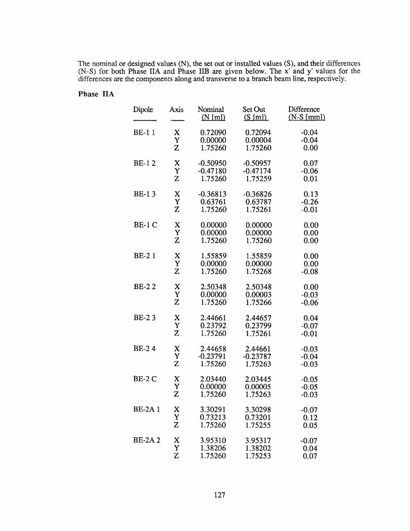
The nominal or designed values (N), the set out or installed values (S), and their differences (N-S) for both Phase IIA and Phase liB are given below. The x' andy' values for the differences are the components along and transverse to a branch beam line, respectively.
Phase IIA
Dipole Axis Nominal SetOut Difference (N [m]) (S [m]) CN-SfmmD
BE-ll X 0.72090 0.72094 -0.04 y 0.00000 0.00004 -0.04 z 1.75260 1.75260 0.00
BE-12 X -0.50950 -0.50957 0.07 y -0.47180 -0.47174 -0.06 z 1.75260 1.75259 0.01
BE-13 X -0.36813 -0.36826 0.13 y 0.63761 0.63787 -0.26 z 1.75260 1.75261 -0.01
BE-l C X 0.00000 0.00000 0.00 y 0.00000 0.00000 0.00 z 1.75260 1.75260 0.00
BE-21 X 1.55859 1.55859 0.00 y 0.00000 0.00000 0.00 z 1.75260 1.75268 -0.08
BE-22 X 2.50348 2.50348 0.00 y 0.00000 0.00003 -0.03 z 1.75260 1.75266 -0.06
BE-2 3 X 2.44661 2.44657 0.04 y 0.23792 0.23799 -0.07 z 1.75260 1.75261 -0.01
BE-24 X 2.44658 2.44661 -0.03 y -0.23791 -0.23787 -0.04 z 1.75260 1.75263 -0.03
BE-2C X 2.03440 2.03445 -0.05 y 0.00000 0.00005 -0.05 z 1.75260 1.75263 -0.03
BE-2A 1 X 3.30291 3.30298 -0.07 y 0.73213 0.73201 0.12 z 1.75260 1.75255 0.05
BE-2A2 X 3.95310 3.95317 -0.07 y 1.38206 1.38202 0.04 z 1.75260 1.75253 0.07
127

BE-2AC X 3.71504 3.71504 0.00 y 0.96998 0.96998 0.00 z 1.75260 1.75250 0.10
BE-3 1 X 13.04986 13.04975 0.11 y 0.00000 -0.00007 0.07 z 1.75260 1.75257 0.03
BE-3 2 X 13.34982 13.34971 0.11 y 0.00000 0.00001 -0.01 z 1.75260 1.75260 0.00
BE-3 3 X 13.92836 13.92836 0.00 y 0.22678 0.22678 0.00 z 1.75260 1.75263 -0.03
BE-3 4 X 14.14847 14.14847 0.00 y 0.43053 0.43054 -0.01 z 1.75260 1.75265 -0.05
BE-3 C X 13.68360 13.68349 0.11 y 0.00000 0.00010 -0.10 z 1.75260 1.75261 -0.01
BE-41 X 22.57348 22.57327 0.21 y 0.00000 -0.00008 0.08 z 1.75260 1.75263 -0.03
BE-42 X 22.87329 22.87308 0.21 y 0.00000 -0.00004 0.04 z 1.75260 1.75261 -0.01
BE-4 3 X 23.45166 23.45166 0.00 y 0.22681 0.22681 0.00 z 1.75260 1.75262 -0.02
BE-44 X 23.67182 23.67182 0.00 y 0.43070 0.43071 -0.01 z 1.75260 1.75259 0.01
BE-4C X 23.20697 23.20676 0.21 y 0.00000 0.00000 0.00 z 1.75260 1.75261 -0.01
Quadrupole Axis Nominal Set Out Difference (N [m]) (N [m]) (N-S [mm])
QE-3A X 4.56640 4.56627 0.13 y 0.00000 0.00002 -0.02 z 1.75260 1.75252 0.08
QE-3B X 4.97890 4.97898 -0.08 y 0.00000 0.00002 -0.02 z . 1.75260 1.75250 0.10
128

QE-3C X 5.39140 5.39144 -0.04 y 0.00000 0.00003 -0.03 z 1.75260 1.75251 0.09
QE-4A X 6.42930 6.42929 0.01 y 0.00000 0.00006 -0.06 z 1.75260 1.75256 0.04
QE-4B X 6.84180 6.84188 -0.08 y 0.00000 -0.00001 -0.01 z 1.75260 1.75255 0.05
QE-4C X 7.25430 7.25436 -0.06 y 0.00000 -0.00003 0.03 z 1.75260 1.75256 0.04
QE-5A X 8.29220 8.29212 0.08 y 0.00000 0.00003 -0.03 z 1.75260 1.75257 0.03
QE-5B X 8.70470 8.70481 -0.11 y 0.00000 0.00003 -0.03 z 1.75260 1.75261 -0.01
QE-5C X 9.11720 9.11726 -0.06 y 0.00000 0.00005 -0.05 z 1.75260 1.75259 0.01
QE-6A X 11.05505 11.05498 0.07 y 0.00000 0.00001 -0.01 z 1.75260 1.75259 0.01
QE-6B X 11.39255 11.39251 0.04 y 0.00000 0.00007 -0.07 z 1.75260 1.75257 0.03
QE-7A X 14.64249 14.64248 0.01 y 0.00000 0.00001 -0.01 z 1.75260 1.75264 -0.04
QE-7B X 14.97999 14.97998 0.01 y 0.00000 0.00006 -0.06 z 1.75260 1.75256 0.04
QE-8A X 15.95499 15.95497 0.02 y 0.00000 0.00000 0.00 z 1.75260 1.75263 -0.03
QE-8B X 16.29249 16.29248 0.01 y 0.00000 -0.00002 0.02 z 1.75260 1.75262 -0.02
129

QE-9A X 19.26588 19.26586 0.02 y 0.00000 0.00004 -0.04 z 1.75260 1.75260 0.00
QE-9B X 19.60338 19.60338 0.00 y 0.00000 0.00001 -0.01 z 1.75260 1.75261 -0.01
QE-lOA X 21.42838 21.42843 -0.05 y 0.00000 0.00005 -0.05 z 1.75260 1.75259 0.01
QE-lOB X 21.76588 21.76582 0.06 y 0.00000 0.00007 -0.07 z 1.75260 1.75265 -0.05
QE-11 A X 25.01591 25.01594 -0.03 y 0.00000 -0.00001 0.01 z 1.75260 1.75263 -0.03
QE-11 B X 25.35341 25.35347 -0.06 y 0.00000 0.00003 -0.03 z 1.75260 1.75262 -0.02
QE-19A X 4.70825 4.70814 0.11 X' 0.12 y -1.54378 -1.54372 -0.06 Y' 0.00 z 1.75260 1.75259 0.01
QE-19B X 5.06548 5.06540 0.08 X' 0.08 y -1.75005 -1.75002 -0.03 Y' 0.01 z 1.75260 1.75258 0.02
QE-19C X 5.42271 5.42276 -0.05 X' -0.04 y -1.95631 -1.95631 0.00 Y' -0.02 z 1.75260 1.75260 0.00
QE-20A X 4.52131 4.52137 -0.06 X' -0.01 y 2.36563 2.36561 0.02 Y' 0.06 z 1.75260 1.75262 -0.02
QE-20B X 4.72765 4.72760 0.05 X' 0.10 y 2.72281 2.72271 0.10 Y' 0.06 z 1.75260 1.75263 -0.03
130

QE-20C X 4.93400 4.93394 0.06 X' -0.05 y 3.07999 3.08008 -0.09 Y' -0.10 z 1.75260 1.75259 0.01
QE-21 X 15.31974 15.31987 -0.13 X' -0.26 y 1.51477 1.51495 -0.24 Y' -0.09 z 1.75260 1.75263 -0.03
QE-22A X 18.36946 18.36948 -0.02 X' -0.06 y 4.33788 4.33794 -0.06 Y' -0.03 z 1.75260 1.75261 -0.01
QE-22B X 18.67217 18.67211 0.06 X' 0.04 y 4.61810 4.61811 -0.01 Y' -0.05 z 1.75260 1.75258 0.02
QE-22C X 18.97488 18.97494 -0.06 X' 0.00 y 4.89832 4.89826 0.06 Y' 0.08 z 1.75260 1.75256 0.04
QE-23 X 24.84267 24.84292 -0.25 X' -0.24 y 1.51505 1.51514 -0.09 Y' 0.10 z 1.75260 1.75260 0.00
QE-24A X 28.25858 28.25863 -0.05 X' -0.08 y 4.67859 4.67866 -0.07 Y' -0.02 z 1.75260 1.75260 0.00
QE-24B X 28.56123 28.56112 0.11 X' 0.15 y 4.95888 4.95878 0.10 Y' 0.00 z 1.75260 1.75263 -0.03
QE-24C X 28.86388 28.86392 -0.04 X' -0.04 y 5.23916 5.23917 -0.01 Y' 0.02 z 1.75260 1.75262 -0.02
131

Phase liB
Dipole Axis Nominal SetOut Difference (N[m]) (N[m]) (N-S [mm])
BE-61 X 35.77147 35.77146 0.01 y 0.0 0.00009 -0.09 z 1.75260 1.75256 0.04
BE-62 X 36.07145 36.07144 0.01 y 0.0 0.00007 -0.07 z 1.75260 1.75256 0.04
BE-63 X 36.64967 36.64966 0.01 y 0.22659 0.22664 -0.05 z 1.75260 1.75256 0.04
BE-64 X 36.86980 36.86978 0.02 y 0.43041 0.43048 -0.07 z 1.75260 1.75258 0.02
BE-71 X 37.70843 y 0.0 0.00000 -0.00 z 1.75260 1.75263 -0.03
BE-7 3 X y z 1.75260 1.75260 0.00
BE-7 6 X 39.65817 39.65821 -0.04 y -1.95024 z 1.75260 1.75257 0.03
BE-81 X 39.65817 39.65821 -0.04 y -5.74551 z 1.75260 1.75260 0.00
BE-8C X 39.65817 39.65822 -0.05 y -6.22140 -6.22143 0.03 z 1.75260 1.75259 0.01
Quadrupole Axis Nominal SetOut Difference IN[m]) (N[m]) (N-S [mm])
QE-12A -x 28.02847 28.02838 0.09 y 0.0 0.00002 -0.02 z 1.75260 1.75259 0.01
QE-12 B X 28.36597 28.36601 -0.04 y 0.0 -0.00004 0.04 z 1.75260 1.75258 0.02
QE-13A X 31.61597 31.61604 -0.07 y 0.0 -0.00001 0.01 z 1.75260 1.75266 -0.06
132

QE-13B X 31.95347 31.95341 0.06 y 0.0 -0.00007 0.07 z 1.75260 1.75261 -0.01
QE-14A X 34.65822 34.65821 0.01 y 0.0 0.00003 -0.03 z 1.75260 1.75260 0.00
QE-14B X 35.14572 35.14586 -0.14 y 0.0 0.00006 -0.06 z 1.75260 1.75262 -0.02
QE-15 A X 39.65817 39.65811 0.06 y -4.51245 -4.51241 -0.04 z 1.75260 1.75264 -0.04
QE-15 B X 39.65817 39.65813 0.04 y -4.99995 -4.99992 -0.03 z 1.75260 1.75258 0.02
QE-16A X 40.64537 40.64538 -0.01 X' -0.09 y -9.16613 -9.16622 0.09 Y' 0.02 z 1.75260 1.75256 0.04
QE-16B X 40.77649 40.77651 -0.02 X' -0.04 y -9.55724 -9.55728 0.04 Y' -0.01 z 1.75260 1.75260 0.00
QE-16C X 40.90760 40.90758 0.02 X' 0.12 y -9.94834 -9.94822 -0.12 Y' -0.02 z 1.75260 1.75256 0.04
QE-17 A X 38.51739 38.51748 -0.09 X' 0.02 y -8.19941 -8.19944 0.03 Y' -0.09 z 1.75260 1.75261 -0.01
QE-17B X 38.31130 38.31142 -0.12 X' 0.07 y -8.55674 -8.55673 -0.01 Y' -0.10 z 1.75260 1.75258 0.02
133

QE-17 C X 38.10522 38.10528 -0.06 X' 0.04 y -8.91407 -8.91406 -0.01 Y' -0.05 z 1.75260 1.75260 0.00
QE-18A X 35.75960 35.75954 0.06 X' 0.01 y -12.98115 -12.98110 -0.05 Y' 0.08 z 1.75260 1.75260 0.00
QE-18 B X 35.55352 35.55347 0.05 X' 0.02 y -13.33848 -13.33843 -0.05 Y' 0.07 z 1.75260 1.75264 -0.04
QE-18 C X 35.34743 35.34734 0.09 X' -0.03 y -13.69581 -13.69579 -0.02 Y' 0.09 z 1.75260 1.75259 0.01
QE-25 X 38.04101 38.04092 0.09 X' 0.07 y 1.51495 1.51494 0.01 Y' 0.05 z 1.75260 1.75261 -0.01
QE-26A X 41.45718 41.45719 -0.01 X' -0.01 y 4.67816 4.67817 -0.01 Y' 0.00 z 1.75260 1.75258 0.02
QE-26B X 41.75986 41.75990 -0.04 X' -0.06 y 4.95843 4.95847 -0.04 Y' 0.00 z 1.75260 1.75261 -0.01
QE-26C X 42.06253 42.06258 -0.05 X' -0.06 y 5.23869 5.23873 -0.04 Y' 0.00 z 1.75260 1.75263 -0.03
QE-27 A X 41.41442 41.41448 -0.06 y 0.0 -0.00003 0.03 z 1.75260 1.75256 0.04
134

QE-27B X 41.90192 41.90196 -0.04 y 0.0 -0.00002 0.02 z 1.75260 1.75264 -0.04
QE-28A X 41.57749 41.57738 0.11 X' 0.12 y -1.85666 -1.85662 -0.04 Y' 0.02 z 1.75260 1.75259 0.01
QE-28 B X 41.99966 41.99963 0.03 X' 0.05 y -2.10043 -2.10038 -0.05 Y' 0.03 z 1.75260 1.75257 0.03
135


Appendix II
(Difference in Coordinates Between Original Control
and the Combined Adjustments for Phase llA)
136


The coordinate differences between the original control network survey adjustment (X0 , Y 0 ,
and Z0) and those determined from the simultaneous adjustment (Xc, Y c• and Zc) containing the combined original control, setting out, and the "wing target" observations.
Station
BEl-l BEl-2 BEl-3 L020-33 L038-33 L060-33 L060-05 L080-20 Ll00-26 Ll00-05 L120-28 L140-28 Ll40-05 Ll54-28 L180-28 L180-05 L200-28 L220-28 L220-05 L240-28 L266-28 L266-05 L280-28 L300-28 L300-05 L320-28 L340-28 L340-05 L360-28 L381-28 L381-05 L400-28 L420-28 L420-05 L440-28 L460-28 L460-05 R020-33 R020-07 R032-20 R060-33 R060-05 R080-28 Rl00-28 Rl00-03 R120-28 R136-28
X0 -Xc (mm)
-0.009 0.017 0.005
-0.020 -0.025 -0.030 -0.011 0.000 0.071 0.064 0.096 0.114 0.107 0.123 0.150 0.138 0.147 0.159 0.164 0.192 0.200 0.205 0.212 0.227 0.227 0.243 0.258 0.259 0.272 0.286 0.285 0.298 0.306 0.306 0.314 0.321 0.321
-0.045 -0.017 -0.032 -0.064 -0.040 -0.055 0.018 0.008 0.068 0.091
137
-0.005 0.006
-0.006 -0.002 0.003 0.005 0.049 0.069 0.078 0.092 0.085 0.079 0.090 0.084 0.051 0.054 0.056 0.070 0.060 0.083 0.076 0.069 0.072 0.064 0.062 0.059 0.050 0.050 0.039 0.032 0.032 0.025 0.020 0.020 0.015 0.010 0.011 0.062 0.057 0.078 0.122 0.123 0.126 0.119 0.086 0.125 0.112
Zo-Zc(mm)
0.018 -0.001 0.001
-0.012 -0.009 -0.019 -0.023 -0.008 0.000
-0.030 0.017 0.029
-0.013 0.041 0.017 0.011 0.019 0.016 0.040 0.024 0.015
-0.009 0.011 0.007
-0.002 0.008 0.011
-0.007 0.010 0.009
-0.005 0.008 0.007
-0.002 0.007 0.007
. -0.001 -0.032 0.005
-0.038 -0.018 -0.024 0.028 0.032
-0.024 0.037 0.024

R136-11 0.093 0.111 -0.011 R160-28 0.115 0.081 0.024 R177-28 0.128 0.080 0.018 R177-03 0.120 0.067 -0.011 R196-26 0.121 0.065 0.005 R220-28 0.111 0.004 0.026 R220-03 0.128 0.018 0.000 R240-28 0.127 -0.018 0.033 R260-28 0.165 -0.006 0.026 R260-03 0.163 0.019 -0.017 R272-28 0.176 -0.021 0.034 R300-28 0.216 0.001 0.014 R300-03 0.206 -0.012 -0.017 R320-28 0.231 -0.006 0.009 R343-28 0.246 -0.015 0.011 R343-03 0.246 -0.012 -0.007 R360-28 0.258 -0.014 O.Oll R380-03 0.273 -0.013 -0.006 R395-30 0.281 -0.013 0.010 R410-30 0.288 -O.Oll 0.009 R420-03 0.291 -0.011 -0.003 R422-28 0.292 -0.012 0.008 R440-28 0.300 -0.012 0.007 R460-28 0.305 -0.013 0.006 R460-03 0.304 -0.014 -0.001 AXW35 0.075 -0.008 -0.007 AXWEND 0.325 0.000 0.015 FLAX1 -0.049 0.045 0.030 FLAX2 0.146 0.054 0.006 FLAX3 0.182 0.054 -0.011 FLAX5 0.246 0.033 -0.010 FLAX6 0.283 0.018 -0.006 FLAX? 0.304 0.008 -0.005 RM101-23 0.323 0.027 -0.009 RM102-03 0.335 0.035 0.020 RM103-24 0.331 0.027 0.006 RM104-03 0.331 0.027 0.015 RM105-30 0.297 0.012 -0.004 RM106-03 0.292 0.014 -0.004 RM107-30 0.277 0.020 0.003 RM108-03 0.262 0.013 0.001 RM109-29 0.236 0.036 0.025 RM110-03 0.238 0.040 0.011 RM111-29 0.228 0.065 0.028 RM112-03 0.235 0.063 0.008 RM113-29 0.197 0.061 0.079 RM201-29 0.285 0.037 0.008 RM202-03 0.284 0.035 0.008 RM203-29 0.281 0.032 0.007 RM204-03 0.283 0.033 0.008 RM205-29 0.278 0.029 -0.002 RM206-03 0.281 0.030 0.009 RM207-30 0.279 0.035 0.000 RM208-05 0.261 0.030 0.007
138
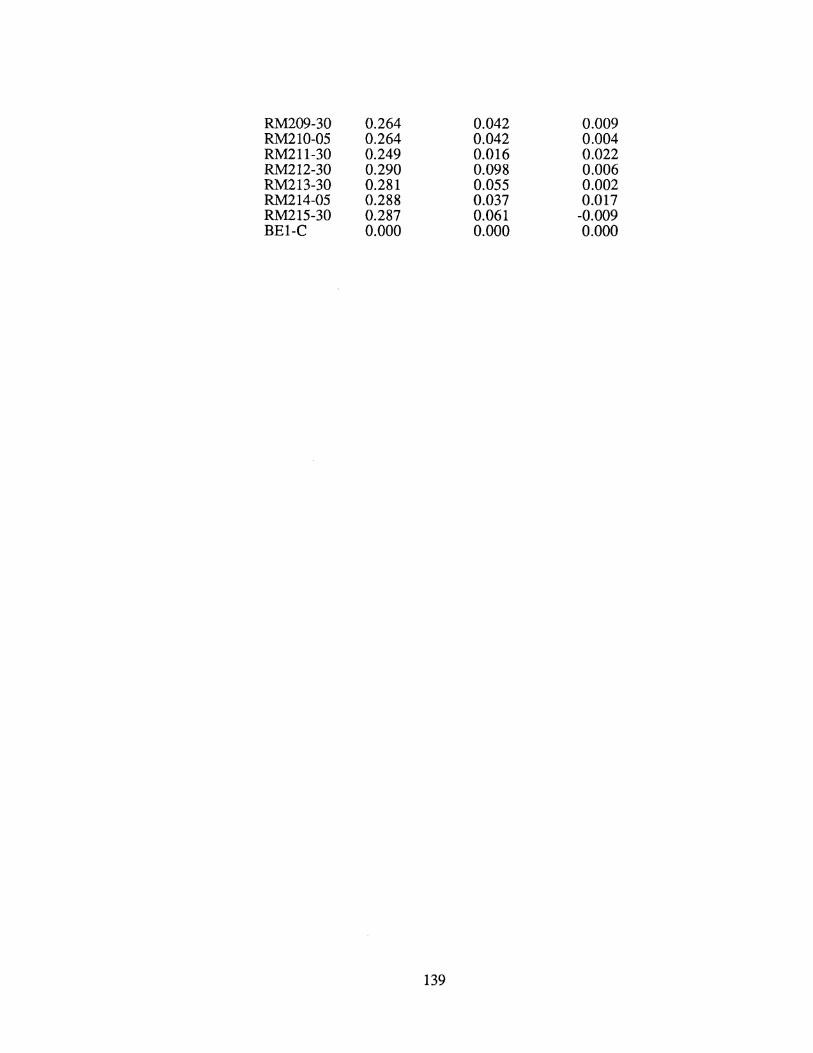
RM209-30 0.264 0.042 0.009 RM210-05 0.264 0.042 0.004 RM211-30 0.249 0.016 0.022 RM212-30 0.290 0.098 0.006 RM213-30 0.281 0.055 0.002 RM214-05 0.288 0.037 0.017 RM215-30 0.287 0.061 -0.009 BE1-C 0.000 0.000 0.000
139


Appendix III
(Plots of Displacements and their 95% Error Ellipses
Between Phase IIA and Phase liB)
140


m N
I
Cl)t
'
\ '
~
141
CD N
1: 0
~ ~ I
N
~]
E

e I
' .
0·
11
142
~]
~· 14 a. ... ... ... w L 0 L L w ~ Ill m £. .., ... " Ill .., £
~ II 0 0 .... a. Ill ... 0
E

~]
CD N (')
I 0 N I N N 'Ot
r3 0::;
'+ '"' ' ..... 01 lt
.jJ E. (J) ... t
@ Q E . 0' -0:.
N CD Cll' X 18, 0 '·'
I< (') (') Ill ~ ~
.,, (') (')' •· ~) ~
Ci. ... .... ..... I IJJ
0 N< L
4J 0 L
' L w ~ Ill
iJ ~ 0)
E. .jJ ... ;r
I• N VI r-. (') .jJ N. 0 1:
I Ill
~~ E. G Q D
0. Ill
0
143

m N
~
m N l
0 ...,. N
B
144
,.... E
...,. N
X
"' "' Ill· d.. ...
......
ll.l
t.. 0 L t..
lJJ<
E
N

~] CD N I
ID
~~ ,... E
ID, N·
I,
)E:
~ E, D) .... , Q.
N' >. ...,
Ill' II• Vi Eli. ... " " W·
1:.. o· 1:.. 1:..
W•
·~ sn. Oj\
E. ..S· ... Ji·
Ill) +' E: q: E: Q' t:J' 0> ...... Eli. llll ....
C•
Ill (1l N 0 I I
0 0 ID 10 N N w oc~
E
rJ
145

ID N I
~
ID N I
N
~
146
~]
"' E
ID_ N
•• M
Gl II
&. ... ..... ..... w t. 0 t. 1:. w ).( U1i Cl'
L .., -~ Cll .., r: II E g· 0 ..... Q.. Cll
c
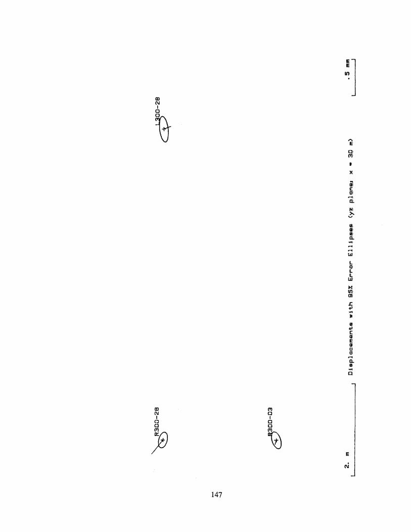
~] m N I
0
\1 " s Ql l"'i•
I'
M
i £ oi ....,, a. N1 >.
v
ca, 111 IIJ; ll. ....
.....
..... w L 0· L L W'
M
""' (Jj;
£. .., ... ~
• .., £ Q E Q u 0 ..... a. • ... 0
m ('I) N 0 1 I
0 0 0 0
) \J E . N
147
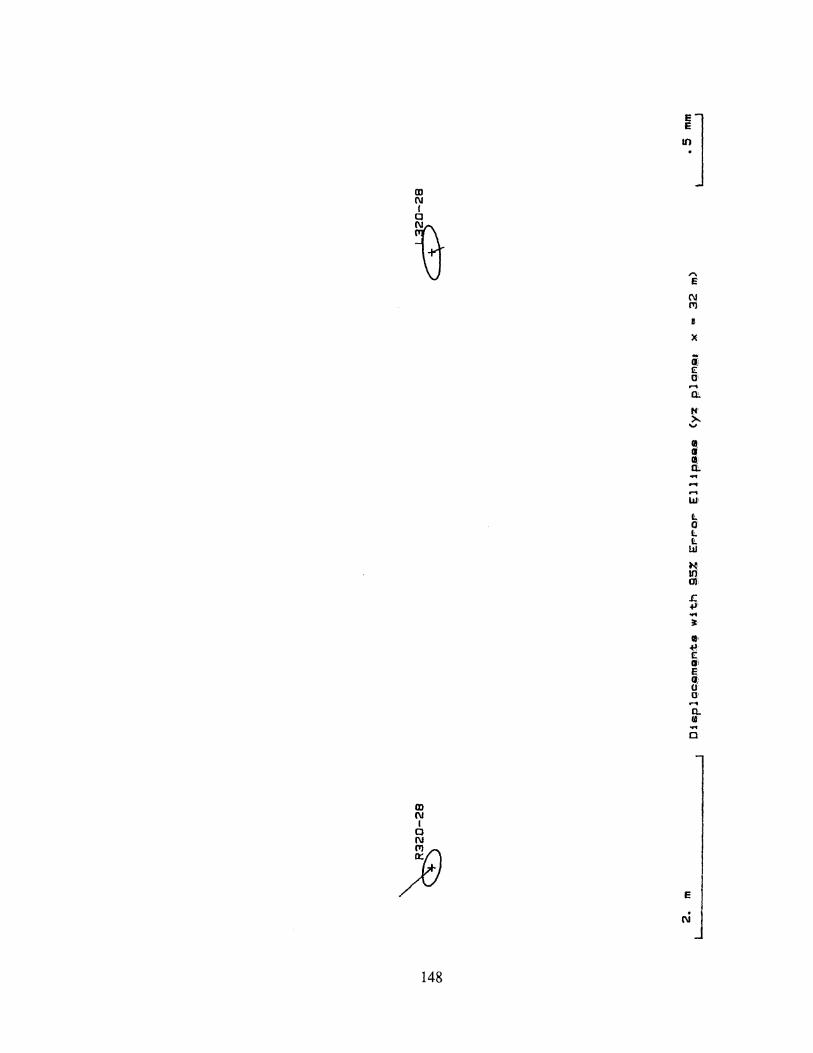
CD N I
~
CD N I
0
)
148
~]
X
i E I]!
..... a
Ill• +!· E Ql E G; 0 I]• .... n. 14
0
E
. N

m N I
0
~
m N I
I'll
~ 149
(I') 0 I
\1
~]
,.., E
'-t I'll
li
)t
• IS' 0\ ~-
n. 1'1' :>. ..,
II .. , Ill! t1. ... --W'
,.
t. 0' L 1!.
Wi
w· 111' Of .
.c. ~ ... • lllj
"" £: ~· E' II' O· 0 .... Q.. .. ... a
E

m N I
0
~
m N I
0 (()
~
150
~]
,.,. E
(() l1i
£ .jJ ... J:
18 .jJ c 0 E
3 0
n. II .... 0
E
1\i

III N I
151
('I) a I
0 III
'(]
~]
" E
III C'l
1:
X
;. £ u
... r"1 .... w 1:. 0 t. 1:. w ~ If) ai
£. +)' ..... ~
ra +> £: II E (J 0 D .... a. 0
a

0 ('I) I
~ 152
~]
,.... E
0 'f
I·
X
i c a· .... a:.
Ill; G! Ill Q;. .... .... .... w t.. 0 t. t. w N Ill m J:. +I .... " II;
.f!' t 0; E: 0 u 0 .... 0:. 0 ... 0

m
~] N I
Q
~ " E
C'll!
""' ,, X
... IJ) c (Jl .... a N' >-"' Ill. IJ Ill a
.-1 .... LIJ
L 0• L £.
L!Ji
N
g?. £. .fJ ... • II +' c Q' E IJ• Q D ..... a. II ....
Q
am ITl ITlN Q I I I ON N ,....N N
'\~ ..,.
\2) E
N
153

(D N I
~
154
~]
I!
..... 1.1.1
t. 0 t.
Ji ~ tn 01
£. .., ... •
' 1: Cl e 8 ..... CL. Ill ... 0

m N I
~
m N I
0
~
155
(Y) 0 I a 10
"" ~
~]
ii' E' 0' ..... n.
18 Ill' llj 0:. ....
......
...... w L d t. 1!.
W•
~ lfl 01
.£:. ..,, .... ~
Ul, .., E II E
3 a .... 0. II ... a
E