Master’s thesis · 30 hec · Advanced level European Erasmus Mundus Master Program: Agricultural Food and Environmental Policy Analysis (AFEPA) Degree thesis No 963 · ISSN 1401-4084 Uppsala 2015

Integration Assessment of Regional Yam Markets in Ghana A Spatial Price Analysis

Noah Larvoe

Integration Assessment of Regional Yam Markets in Ghana A Spatial Price Analysis

Noah Larvoe

Supervisor: Yves Surry, Swedish University of Agricultural Sciences,

Department of Economics Assistant supervisor: Bruno Henry de Frahan, Universite Catholique de Louvain, Department of Rural Economy Examiner: Sebastien Hess, Swedish University of Agricultural Sciences, Department of Economics Credits: 30 hec Level: A2E Course title: Independent Project/Degree Project in Economics Course code: EX0537 Programme/Education: European Erasmus Mundus Master Program: Agricultural Food and Environmental Policy Analysis (AFEPA) Faculty: Faculty of Natural Resources and Agricultural Sciences Place of publication: Uppsala Year of publication: 2015 Name of Series: Degree project/SLU, Department of Economics No: 963 ISSN 1401-4084 Online publication: http://stud.epsilon.slu.se Key words: Autoregressive, Impulse Response, Integration, Regional Markets, Symmetric Threshold Cointegration, Price Transmission, Yam

iii

Abstract

World food price hikes in 2007/2008 and 2012 plunged several people into hunger and poverty in

developing countries. The situation stimulated responses from policy makers in some of these countries by

trying to boost local production of crops in which they are self-sufficient. Integrated agricultural marketing

systems are needed in the process in order to ensure efficient distribution and improvement in welfare of

all actors involved in the consumption and production chain. The food balance sheet for Ghana shows that

the country is self-sufficient in root and tuber crops such as cassava and yam. The main objective of the

study is to determine the extent to which regional yam markets are integrated. Using monthly wholesale

price series from 2006 to 2013, the study assesses the integration dynamics between five regional yam

markets in Ghana. From the consistent threshold autoregressive model of cointegration, the study found

that regional yam markets in Ghana are integrated. Thus, prices between local markets (Kumasi, Tamale,

Techiman and Wa) and the reference market (Accra) are interdependent on each other both in the long-run

and short-run, although there were some evidences of unidirectional interdependence. The Kumasi-Accra,

Tamale-Accra and Techiman-Accra market pairs exhibited asymmetric adjustments whiles Wa-Accra

market pair exhibited a symmetric adjustment. From the impulse response estimations, we found that

different time periods are required for equilibrium to be restored when there is a shock in one pair of the

four market combinations considered. The speed of adjustments was also dependent on the direction

(positive or negative) of the shock or deviation. Overall, adjustment periods range between 8 months to

27months with the minimum adjustment time occurring between Techiman-Accra. In some cases, price

shocks were persistent and required a long time to adjust. The integration found between regional markets

could be attributed to improvement in ICT tools, such as mobile phones, as has been noted in some

reviewed studies. The high and persistent adjustment times recorded between some market pairs may

however, be attributed to comparatively low value-to-volume ratio of yam compared to other market

commodities. This makes the cost of transportation a major portion of its price setting.

iv

Table of Contents Abstract .......................................................................................................................................... iii

List of tables ................................................................................................................................... vi

List of figures ................................................................................................................................. vi

List of abbreviations ..................................................................................................................... vii

Acknowledgement ....................................................................................................................... viii

Dedication ...................................................................................................................................... ix

Chapter 1- Introduction ................................................................................................................... 1

1.1 Background ........................................................................................................................... 1

1.2 Problem statement ................................................................................................................. 4

1.3 Study objectives .................................................................................................................... 5

1.4 Research hypothesis and relevance of study ......................................................................... 5

Chapter 2-Literature review ............................................................................................................ 7

2.1 Concepts of market integration and its application to spatial markets ................................. 7

2.2 Models of spatial price analysis .......................................................................................... 10

2.3 Review of similar studies .................................................................................................... 20

2.4 Lessons and conclusion from review .................................................................................. 26

Chapter 3- Research methodology ................................................................................................ 28

4.1 Study area and data collection ........................................................................................ 28

3.2 Analytical methods ............................................................................................................. 29

3.2.1 Test for unit roots in the presence of structural breaks ................................................ 30

3.2.2 Modelling long run relationship between regional markets ........................................ 32

3.2.3 Test for asymmetry ...................................................................................................... 33

3.2.4 Modelling short-run dynamics of price linkages ......................................................... 35

Chapter 4 - Results and discussion ............................................................................................... 38

4.1Variations, seasonality and trend in market prices .............................................................. 38

4.2 Test for structural breaks and stationarity ........................................................................... 40

4.3 Determining long-run relationships between regional markets .......................................... 42

4.4 Threshold cointegration and asymmetric adjustment ......................................................... 44

4.5 Short-run relationships between regional markets .............................................................. 49

v

4.6 Impulse response estimation ............................................................................................... 51

Chapter 5 - Summary and conclusion ........................................................................................... 55

REFERENCES ............................................................................................................................. 57

Appendix A ................................................................................................................................... 63

vi

List of tables

Table 4.1 Descriptive statistics of wholesale nominal prices ....................................................... 39

Table 4.2 HEGY test for seasonality in price series ..................................................................... 40

Table 4.3 Test for unit root by ADF and PP ................................................................................. 41

Table 4.4 Zivot-Andrews test unit root test for structural breaks ................................................. 41

Table 4.5 Engle-Granger cointegration test results (first stage) ................................................... 43

Table 4.6 Test for stationarity in the residuals .............................................................................. 43

Table 4.7 Results of Johansen cointegration test .......................................................................... 44

Table 4.8 Threshold autoregressive results ( = 0) ....................................................................... 45

Table 4.9 Momentum threshold autoregressive model ( = 0) ..................................................... 45

Table 4.10 Consistent threshold autoregressive result .................................................................. 47

Table 4.11 Consistent momentum threshold autoregressive results ............................................. 47

Table 4.12 Vector error correction model results ......................................................................... 50

Table A.1 Critical values for TAR and MTAR test (= 0) ........................................................... 64

Table A.2 Critical values for TAR and MTAR test ( is unknown) ............................................. 64

List of figures

Figure 1.1 Regional map of Ghana ................................................................................................. 1

Figure 3.1 Marketing routes of yam in Ghana. ............................................................................. 28

Figure 3.2 Summary of research methodology ............................................................................. 37

Figure A.1 Response of KU market to shock in AC market price ............................................... 63

Figure A. 2 Response of AC market to shock in KU market price .............................................. 63

vii

List of abbreviations

AC Accra market

ADF Augmented Dickey-Fuller test

AEG Augmented Engel-Granger test

AIC Ackaike Information Criterion

ARCH Autoregressive Conditional Heteroscedasticity

BIC Bayesian Information Criterion

FAOSTAT Food and Agriculture Organization Statistics

FASDEP Food and Agricultural Sector Development Policy

GSS Ghana Statistical Service

ICT Information Communication Technology

IFAD International Fund for Agriculture

IMC Index of Market Connectedness

KU Kumasi market

LOP Law of One Price

PP Philips Perron

RTIMP Root and Tuber Improvement and Marketing Programme

TA Tamale market

TAR Threshold Autoregressive

TE Techiman Market

SRID-MoFA Statistics Research and Information Directorate of Ministry of Food and Agriculture

M-TAR Momentum Threshold Autoregressive

PBM Parity Bound Model

VAR Vector Autoregressive

VECM Vector Error Correction Model

WA Wa market

USAID United States Agency for International Development

viii

Acknowledgement

I will always be grateful and thankful to God for His unmerited favor, grace and mercies that have seen

me through to this far in my studies.

I would like to express my heart-felt gratitude to my supervisor, Prof. Yves Surry for all the time he took

off his busy schedules to offer me all the useful criticisms, suggestions and comments throughout this

research. I am also thankful to Prof. Bruno de Frahan, the co-supervisor of this thesis. These two

Professors have also been instrumental in shaping my career even before I could finish my master’s

programme. I say God richly bless you.

I would also like to thank the European Union for the wonderful Erasmus Mundus scholarship which

made my dream to study in Europe a reality.

My very supportive family cannot be left out. They have stood behind me right from infancy especially

my dad Robert Larvoe and my mum Elizabeth Larvoe together with all my siblings. I am so grateful for

the enabling environment you created for me regardless of my mistakes.

To all the amazing Professors and course mates, I met in AFEPA program in Universite Cathoque de

Louvain and Swedish University of Agricultural Sciences, I say thank you all for making my stay in

Europe a memorable experience. My deep appreciation also goes to Auntie Georgina Nkunu of MoFA for

her assistance during my data collection, Elder David A. Quarshie, Pastor Agbozo, Mr James Lavoe and

Uncle Dennis Awittor for your advice and the various supports throughout my studies.

Finally, to Elder James Arthur, Emmanuel Vifa Larvoe, Enoch Tieku, Samuel Doe, Mary Amponsah

Larvoe and all friends, I say I am highly indebted to you all and God bless you.

ix

Dedication

I dedicate this work to the entire family of Rev. M. B. Agyekum. I believe aside one’s biological parents,

everyone on earth needs people who will support, care and stand by them at a point in time. That is what I

found in this wonderful family. God richly bless you all.

x

1

Chapter 1- Introduction

1.1 Background

The Agricultural sector in Ghana continues to be one of the most important sectors despite presently

being overtaken by the services and the industrial sectors in terms of their contribution to Gross Domestic

Product. The sector is currently ranked third and contributes 22% of the country’s Gross Domestic

Product (GSS, 2014) with crops accounting for about 77% of this figure. Agriculture also employs an

estimated 42% of Ghana’s overall working population and 76% of total rural households (GSS, 2010).

Root and tuber crops form part of many staple foods and account for major calorie intake in Ghana.

According to SRID-MoFA (2013), the estimated levels of per capita consumption of cassava and yam are

154 and 50 kg/head/year respectively. Cassava accounts for about 22% (Nti & Sackitey, 2010) while yam

accounts for about 16% (Anaadumba, 2013) of the total agricultural Gross Domestic Product.

Yam is therefore, second to cassava in terms of root crop production in Ghana and accounts for about 24

percent of total roots and tubers production in the country (MoFA, 2010). Yam is produced in seven out

of the ten regions in the country. The Brong Ahafo, Northern and Eastern regions are the major

producers. The combined share of these regions make up about 76% of the countrywide production with

the remaining 24% distributed among the remaining 4 regions. See the regional map of Ghana below.

Figure 1.1 Regional map of Ghana

2

The crop takes approximately 8 months to mature and requires about 5 months of rainfall during its

growing period. There are several varieties of yam produced in Ghana, but the most preferred one for

both the domestic and the export markets is the white yam (also known as Pona in Ghana). Just like

cassava, yam cultivation in Ghana is mainly done by smallholder farmers using rudimentary hand tools

making cultivation and harvesting much more labor intensive. According to SRID-MoFA (2013), the

annual production of yam is estimated at 6.7 million metric tons in Ghana with main harvesting periods

starting from August to December. There are, however, lean seasons (period of low harvest activities)

which occur between May and July. As noted by Anaadumba (2013), in many cases, yam producers are

persuaded by traders to harvest their crop early in the season, when prices are very high. Nevertheless,

immature yams are more perishable, which may partly explain why many producers experience high post-

harvest losses.

Although yam is consumed in all parts of Ghana, Aidoo (2009) indicates that yam consumption tends to

be higher in urban areas. He found that boiled yam (known in the local language as ampesi) is the most

preferred yam product in Ghanaian urban centers, followed by pounded yam (fufu). Nonetheless,

depending on the type of yam, it could also be used in variety of ways which includes roasted and fried

yams.

Unlike cassava, Ghana exports a significant amount of yam and it is the leading exporter in the world as

reported by Anaadumba (2013). Data from FAOSTAT shows that export during the 2008 food crisis was

very high indicating its importance to consumers abroad especially many African migrants. Data from the

millennium development authority, as reported by Anaadumba (2013), shows that the United Kingdom,

the USA and the Netherlands are the major destination of yam exports from Ghana. The three countries

together imports 90% of Ghana’s total yam export. Yet, yam exports like other crops, faces many quality

problems arising from poor road network, harvesting and storage processes. This sometimes results in the

spoilage of many tubers before they arrive at their export destination. According to Bancroft (2000), yam

in Ghana is marketed in its original state without any special package or treatments including those

exported. Thus, small restaurants and individual consumers buy the unprocessed yam and prepare them

for consumers and consumption respectively.

Although there have been various forms of support to yam farmers, Anaadumba (2013) asserts that the

value chain remains weak and less developed compared to commodities such as maize or rice. The

marketing chain shows that yam harvested in the Northern Region is mostly transported to Accra through

the Eastern Corridor; either through Hohoe and Akosombo or through Kete Krachi in the Volta region.

Some yams from the Northern region are also transported to Kumasi through Yeji, Atebubu and Ejura

using ferries or to Tamale by road (Anaadumba, (2013). Yams from the Brong Ahafo Region mainly go

3

to Techiman, Kumasi or Accra. Figure 3.1 shows the various routes described above. Yam exporters

normally purchase their commodities directly from farmers or wholesale shops in Accra, but increasing

competition among exporters means most of them are forced to go to production areas as reported by

USAID (2005).

With steadily increasing growth and development in Ghana, the consumption pattern is expected to shift

towards more protein diet, but root and tuber crops will continue to be important, since they form part of

staple foods of major ethnic groups in Ghana. For instance, Anaadumba (2013) highlighted yam as an

important staple food for many Ghanaians, accounting for 11% of total consumption in 2007. The

country is also the leading exporter of yam in West Africa accounting for about 94 % total yam export in

the West Africa region.

Although Ghana is a net importer of food products, the country has a comparative advantage in the

production of roots and tubers which could be built on to enhance food security and increase agricultural

trade. The annual food balance sheet shows that the country has an excess of 6.2 million and 2.1 million

metric tons of cassava and yam respectively (SRID-MoFA, 2013). According to the same report, the

mean annual production growth rate of cassava and yam are estimated at 12.56% and 11.31% respectively

between 2007 and 2012.

Ghana’s agricultural sector specifically, the crop sector, is dominated by smallholder farmers with 90% of

farm holdings being less than 2 hectares in size. However, due to the different climatic conditions in the

country, agricultural production is not evenly distributed. Production of yam is mainly centered in the

northern and central part of Ghana, although they are consumed in all parts of the country. It is therefore

necessary that there is a smooth flow of these crops across the different regions in order to ensure food

sufficiency to all households. To achieve this goal, the country relies heavily on the market system to

transfer food from surplus producing regions to deficit regions. This has been the situation since the

abolition of the state’s involvement in production and distribution in 1990 through liberalization of the

market system. The 2010 population census shows that the urban population has increased to 51% from

44% in 2000 (GSS, 2010). With this increasing rate of urbanization, the market system will continue to be

relevant in the course of food distribution in Ghana and more so since the majority of the population

spends significant portion of their budget on food.

Following the 2007/2008 and 2012 food price hikes, there have been major concerns about food security

especially in developing countries (Godfray et al., 2010). The rise of world grain, livestock and dairy

product prices, which impacts were heavily felt in many developing countries, means developing

4

countries cannot continue to rely on world markets. This is because the transmission of these high world

grain market prices into the domestic markets of developing countries plunged several people into hunger

and poverty (Mittal, 2009).

It is therefore imperative for countries such as Ghana to put in place appropriate policies to boost

production and distribution especially, traditional crops which have long been touted as food security

crops. The main challenge of food distribution remains lack of efficient market system in many countries

(Godfray et al., 2010). In event of price hikes such as the 2007/2008, crops as cassava and yam will be

heavily counted upon to serve many Ghanaians especially the poor households. Nevertheless, the

marketing system in Ghana faces many challenges which include lack of proper road network, inadequate

product development for effective utilization of farm produce, and generally weak commodity value

chains.

As major staples in Ghana, root crops have been the targets of several government policy frameworks in

order to boost production and market access. The recent of such policies is the Root and Tuber

Improvement and Marketing Programme (RTIMP) funded by International Fund for Agriculture (IFAD)

which covered a period of 8 years between 2007 and 2014. The program sought to support root and tuber

production and increase market linkages between regions. All these efforts are geared towards ensuring

that the country maintains a high level of production to meet local consumption requirements and in some

cases export as well as industrial use especially cassava.

1.2 Problem statement

Although production of food to meet local demand remains a major challenge in many developing

countries, the issue of distribution through the market system poses a greater challenge to attaining food

security in these countries (Godfray et al., 2010). The issue is not different in Ghana. In trying to

achieve food security status in Ghana, the Ministry of Food and Agriculture has pursued several policies

over the years.

As highlighted by the FASDEP II (2008), the broad strategy for the attainment of food security is to focus

on the development of five staple crops (maize, rice, yam, cassava and cowpea) on national and agro-

ecological levels. The ministry however, identified lack of efficient market systems in the sector and has

since been pursuing various policies to attain this efficiency through the FASDEP II since 2008. Under

this programme, one of the main objectives has been to increase competitiveness and enhance integration

between domestic markets and also with international markets. Thus, improving accessibility from farm

to market centers and between regions is clearly a major priority in Ghana. But how have these policies

5

improved the situation of especially root and tuber markets integration? This is an important question

because one of the main challenges identified in the marketing of agricultural products during the drafting

of FASDEPII were challenges such as poor nature of roads to production centers, inadequate market

information, leading to weak market integration between local, districts, regional markets. Poor rural road

infrastructure limits the effective distribution of food and lowers producer prices.

According to Acquah et al. (2012), integrated markets are important avenues of raising the income level

of farmers and promoting the economic development of a country. They also asserted that in the state of

well integrated markets, farmers allocate their resources according to their comparative advantage and

invest in modern farm inputs to obtain enhanced productivity and production. Also, food becomes

available and affordable thereby improving the food security status of households. This is very necessary

in Ghana since almost all families supplement their food requirements with significant amounts of

purchased staple crops. A well-integrated market is therefore needed to efficiently supply all households

in order to achieve food security status in all parts of the county. Investigation of root and tuber crops

integration is therefore vital since these crops are considered as food security crops in Ghana. Thus,

integration can be regarded as a way of assessing efficiency of the root and tuber markets and for that

matter a way of assessing the disparity between welfare of producers and consumers of the commodity in

the different regions in Ghana.

This study therefore seeks to analyze comprehensively the extent of regional yam market integration by

answering the following questions: To what extents do price shocks of yam in one regional market in

Ghana affect other regional markets both in the short run and the long run? Are these shock transfers

symmetric or asymmetric? At what speed are these shocks transmitted?

1.3 Study objectives

The main objective of this study is to assess the extent of integration of regional yam markets in Ghana.

This will be achieved by the following specific objectives:

i. To determine short and long-run price co-movement of regional yam market in Ghana

ii. To determine the type of adjustment between regional market prices after price shocks and,

iii. To determine the speed of price shock transmission from one regional market to another.

1.4 Research hypothesis and relevance of study

Following several government interventions and policies in the root and tuber sector in pursuance of food

security status as part of the Millennium Development Goal One in Ghana, the regional yam markets are

expected to be spatially integrated. This means a price shock in one regional market will be transmitted

into all other markets eventually. However, due to infrastructural bottlenecks such as bad road network

6

and bulky nature of root and tuber crops, price shock adjustment is expected to be somewhat slow. The

study therefore seeks to test the hypothesis that:

Regional yam markets are perfectly integrated with symmetric response since these regions are

interdependent on each other. This means even though short-run prices may drift apart, long-run price

between regional markets will exhibit similar trends. We also predict slow adjustment to equilibrium

between markets infrastructural bottlenecks.

The relevance of this study is summarized by the statement below quoted and acknowledged as such:

Market integration is a central issue in many contemporary debates concerning market liberalization. It

is perceived as a precondition for effective market reform in developing countries: “Without spatial

integration of markets, price signals will not be transmitted from urban food deficit to rural food surplus

areas, prices will be more volatile, agricultural producers will fail to specialize according to long term

comparative advantage and gains from trade will not be realized” (Baulch 1997, p. 477). The knowledge

of price mechanisms reduces uncertainty for policy-makers and the risk of duplication of interventions in

two markets (Goletti et al., 1995)

To add to this argument in Ghana, studies on spatial market integration have mostly focused on the cereal

sector especially rice and maize. The root crop sector specifically, yam is chosen because the country is

self-sufficient and this means such commodities will be heavily relied upon in the event of escalating

world prices of grain and dairy products as occurred in 2008 and 2012. Many previous studies have also

not explored the causes and determinants of market integration. In addition, the concept of market

integration also needs to be updated frequently in order to inform policy makers the current trend and for

that matter how producers and consumer welfare can be improved through national and regional market

policies. The study will also add up to the already existing pool of literature on spatial market integration.

The study is structured into five chapters. The first chapter above presents the background, research

problem and objectives of the study as already seen. The next chapter (chapter two) reviews various

market integration studies by analyzing the different models and their applications. Similar studies in

Ghana and other countries are also reviewed with emphasis on their results and how they differ from this

study. Chapter three details out the research methodology used to achieve the study objectives whereas

we present the results and discussion in chapter four. The last chapter summarizes the whole study and

gives conclusions.

7

Chapter 2-Literature review

2.1 Concepts of market integration and its application to spatial markets

According to Hopcraft (1987), an indirect method of analyzing market efficiency is to test for market

integration. In some cases market integration has been used in the same context as market efficiency.

Some spatial price literatures have however distinguished between the two terms, though they agree the

two are related to some extent (Barret and Li, 2002; Barrett, 2005; Fackler and Goodwin, 2001). Although

there has been no formal definition of the term, Fackler and Goodwin (2001) suggest market integration

as a measure of degree to which demand and supply shocks arising in one region are transmitted to

another region. Market integration is therefore a measure of extent rather than a specific relationship.

Thus, two markets are said to be integrated when a particular shock which shifts for instance, excess

demand and for that matter prices in one market causes some changes in prices in another market.

The extent of integration depends on the price transmission ratio between the two markets. This definition

according to Fackler and Goodwin (2001) clarifies the use of the term in early literature studies which

simply portrayed market integration as commodity price co-movement in different regions. They argue

that price co-movement between different regions could occur for some reasons, although the regions

might not necessarily be linked by any trading network. Barret and Li (2002) also define market

integration as tradability or contestability between markets. The authors describe the phenomenon as the

transfer of Walrasian excess demand from one market to another, they manifest in physical flow of a

commodity and the transmission of price shock from one market to another or both. Thus from this

definition, physical movement of commodity between two markets is a sufficient but not a necessary

condition to demonstrate “tradability” which according to Barret (2005) is the main focus of market

integration in macroeconomics and international trade. He defines tradability as a notion that a good is

traded between two economies, or that market intermediaries are indifferent between exporting from one

nation to another and not doing so. This means positive trade flows are sufficient to illustrate trade market

integration under tradability condition, and prices need not equilibrate between markets. Based on this,

Barrett (2005) pointed out differences between two criteria for conceptualizing market integration:

tradability-based in which trade is a sufficient condition and efficiency-based where trade is neither a

necessary nor sufficient requirement.

Barrett (2005) therefore thinks that market integration conceptualized as tradability is consistent with

Pareto inefficiency. Contestability as a concept of market integration in the absence of trade is when

arbitrageurs face zero marginal returns leaving them indifferent about trading (Barrett and Li, 2002). The

8

contestability idea therefore focuses on maximal exploitation of arbitrage rent and for that matter a

competitive market.

In trying to analyze spatial market, many terms have been used to introduce different concepts in different

literature which need to be highlighted. Terms such as price transmission, volatility and seasonality are

constantly used in spatial price analysis. Spatial arbitrage mentioned earlier in this review is one common

term in such studies.

Spatial arbitrage is a condition in spatial market analysis where prices of a commodity between two

different locations differ exactly by the cost of moving the commodity from the region of lower price to

the region of higher price. This cost is referred to as the transaction cost and it includes all costs such as

transport cost and information costs that are involved in getting the commodity from one location to

another. The spatial arbitrage condition is therefore regarded as a starting point of any model of spatial

price behavior. However, this is an equilibrium condition as asserted by Fackler and Goodwin, (2001) and

hence actual market prices may not follow the condition, but action of arbitrageurs will tend to move

price differences towards the transaction cost in a well-functioning market.

Efficiency of spatially distant markets is therefore based on how potential profitable arbitrage

opportunities are exploited. According to Negassa et al. (2003), when a spatial price differential is less

than the transfer cost in the absence of trade, the efficiency condition holds. There is however,

inefficiency when spatial price differentials are greater than transfer cost in the presence of trade or not.

Market efficiency as asserted by Fackler and Goodwin (2001) is therefore used to motivate empirical

studies of market integration.

Another fundamental concept in spatial market analysis is the Law of One Price (LOP). This is a unique

concept of arbitrage which holds when regional markets that are linked together by trade have a common

unique price abstracting for transaction cost (Fackler and Goodwin, 2001). Yet, Fackler and Goodwin

(2001) noted that there are several versions of the Law of one price. They refer to a situation where some

authors fail to distinguish between LOP and spatial arbitrage as weak LOP. The strong version is where

spatial arbitrage condition holds as equality, thus price between two regions differing only by the

transaction cost.

Market integration should therefore be expected when we observe a strong form of LOP. However,

according to Fackler and Godwin (2001), the term is often used for both strong LOP where there is

perfect market integration and even the weak form of LOP where we have the spatial arbitrage condition.

9

LOP is one reason why market integration cannot be defined simply as price co-movement. This is

because prices that satisfy strong form of LOP may not move together if transport costs are large and

volatile as noted by Fackler and Godwin (2001).

Analysis of spatial market integration of agricultural products is an important concept in many literatures

in Agricultural economics. Agricultural commodities are normally produced in areas where there is

surplus and hence must be moved to areas where there is deficit in supply. Sexton et al. (1991)

highlighted the relevance of spatial market integration as agricultural products are always bulky and/or

perishable and production is mostly concentrated in one location whereas consumption in the other. This

may imply an expensive transportation cost which may cause price not to move together even if a strong

form of LOP is satisfied as noted above. Spatial agricultural commodity markets therefore require careful

and dynamic analysis to establish whether or not they are integrated.

The analysis of market integration in most literature is based on the Enke-Samuelson-Takayama and

Judge (ESTJ) spatial equilibrium model (Barret, 2005). In the ESTJ model, the dispersion of prices in two

locations for identical goods is bounded from above the cost of arbitrage between the markets when the

trade volumes are unrestricted and from below when trade volumes are restricted for example with quota.

Thus, the model assumes that price relationships between spatially competitive markets depend on the

size of the transaction costs. If the difference between prices of two markets is exactly equal to the

transaction cost for a homogenous good, then the two markets are considered very competitive (Barret,

2005). However, if price difference exceeds the transaction costs, then arbitrage condition is created and

profit seeking agents will purchase the commodity from low price surplus markets and sell them in high

price deficit markets as noted by Katengeza (2009).

To illustrate the spatial market integration, consider two spatially distinct markets, market one (M1) and

market two (M2) with prices P1

and P2

respectively and 12

as the transaction cost involved in moving a

homogenous commodity from M1 to M2. Following (Fackler and Goodwin, 2001; Barret, 2005;

Ankamah, 2012), two markets are said to be integrated when P1 = P

2 +

12. Thus, the price in the two

markets should equal each other accounting for the cost of transaction. As implied by the ESTJ model,

this does not mean trade occurs between the two markets. In other words trade is neither a necessary nor

sufficient condition for the attainment of such equilibrium condition. Trade will however occur when P1

- P2 >

12 thus, when the differences in prices exceeds the cost of transaction involved in moving the

commodity between the two markets.

10

One important term worth highlighting is the issue of central or reference market. In many studies

(Alderman 1991; Shively 1996; Amikuzuno 2009, 2010) the choice of the reference markets is based on

which market has net surplus or net deficit of the commodity in question. In most of these studies the net

surplus or producing region is chosen as the reference market. In other studies however, the net

consumption market is used as the reference market as shown in Mensah Bonsu et al. (2011). Regardless

of whether a net consumption or production market is used, the main idea behind the central/reference

market is that it is the shock originating market. Thus, it should have the features such that it is able to

influence other local or regional markets when there is a shock in that market.

2.2 Models of spatial price analysis

Spatial prices analysis models have evolved over the years from simple correlation analysis to presently

more sophisticated models. As researchers identify various problems associated with spatial price

analysis, different models have been used to empirically examine integration of spatial markets in an

attempt to solve some of these problems. This section reviews some of the past techniques that have been

used to address spatial market integration.

Simple correlation or regression techniques

Earlier studies on market integration focused on testing for the Law of One Price using static simple

regression/correlation analysis. In many early empirical studies, authors assumed that spatially integrated

markets share common price linkages. By such an assumption, researchers used simple regression or

correlation analysis to determine the extent to which markets were integrated. Although the

interpretations in regression and correlation differ, the mechanisms involved in their implementation are

similar. According to Hossain and Verbeke (2010), regression analysis of market integration involves

estimating bivariate correlation or regression coefficients between the time series of spot prices of

homogenous good at distinct market places. The technique is based on the equation:

𝑷𝟏𝒕 = 𝜶° + 𝜶𝟏𝑷𝟐𝒕 + 𝜺𝒕 (2.1)

where 𝑃1𝑡 and 𝑃2𝑡 are price series between two markets, o and 1 are parameters to be estimated and

t is the error term. The LOP is then tested based on the necessary condition that o = 0, 1 = 1. This is a

test for the strong form of LOP. However, since this form of LOP rarely occurs, a necessary restriction is

11

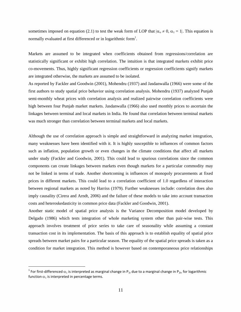
sometimes imposed on equation (2.1) to test the weak form of LOP that o 0, 1 = 1. This equation is

normally evaluated at first differenced or in logarithmic form1.

Markets are assumed to be integrated when coefficients obtained from regressions/correlation are

statistically significant or exhibit high correlation. The intuition is that integrated markets exhibit price

co-movements. Thus, highly significant regression coefficients or regression coefficients signify markets

are integrated otherwise, the markets are assumed to be isolated.

As reported by Fackler and Goodwin (2001), Mohendru (1937) and Jasdanwalla (1966) were some of the

first authors to study spatial price behavior using correlation analysis. Mohendru (1937) analyzed Punjab

semi-monthly wheat prices with correlation analysis and realized pairwise correlation coefficients were

high between four Punjab market markets. Jasdanwalla (1966) also used monthly prices to ascertain the

linkages between terminal and local markets in India. He found that correlation between terminal markets

was much stronger than correlation between terminal markets and local markets.

Although the use of correlation approach is simple and straightforward in analyzing market integration,

many weaknesses have been identified with it. It is highly susceptible to influences of common factors

such as inflation, population growth or even changes in the climate conditions that affect all markets

under study (Fackler and Goodwin, 2001). This could lead to spurious correlations since the common

components can create linkages between markets even though markets for a particular commodity may

not be linked in terms of trade. Another shortcoming is influences of monopoly procurements at fixed

prices in different markets. This could lead to a correlation coefficient of 1.0 regardless of interaction

between regional markets as noted by Harriss (1979). Further weaknesses include: correlation does also

imply causality (Cirera and Arndt, 2006) and the failure of these models to take into account transaction

costs and heteroskedasticity in common price data (Fackler and Goodwin, 2001).

Another static model of spatial price analysis is the Variance Decomposition model developed by

Delgado (1986) which tests integration of whole marketing system other than pair-wise tests. This

approach involves treatment of price series to take care of seasonality while assuming a constant

transaction cost in its implementation. The basis of this approach is to establish equality of spatial price

spreads between market pairs for a particular season. The equality of the spatial price spreads is taken as a

condition for market integration. This method is however based on contemporaneous price relationships

1 For first-differenced 1 is interpreted as marginal change in P1t due to a marginal change in P2t, for logarithmic

function 1 is interpreted in percentage terms.

12

and does not take care of dynamic relationships between a given pair of individual markets (Ankamah,

2012).

Dynamic models

Many studies have therefore resorted to the use of dynamic models due to the nature of price data used in

market integration analysis to address the above problems. The use of dynamic models is also more

important considering the dynamic nature of interregional marketing of especially agricultural

commodities which have large transport costs due to their bulky and perishable nature. This may lead

to significant delivery lags and slow shocks adjustment processes and hence making shocks persistent

according to Fackler and Goodwin (2001). Commonly used dynamic regression models are reviewed

below:

Granger causality test

Ganger causality test is one of the approaches which use a reduced form model to test for spatial market

efficiency. According to Fackler (1996), many spatial models suffer from identification problems because

they involve the use of simultaneous equations. This model however does not require identification. The

model is implemented within a vector auto-correlation regression framework. The regional market price

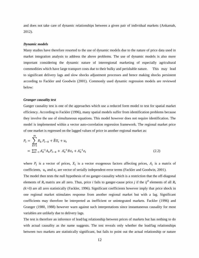
of one market is regressed on the lagged values of price in another regional market as:

𝑃𝑡 = ∑ 𝑅𝑘

𝑚

𝑘=1

𝑃𝑡−𝑘 + �̃�𝑋𝑡 + 𝑢𝑡

= ∑ 𝐴0−1𝐴𝑘𝑃𝑡−𝑘

𝑚𝑘−1 + 𝐴0

−1𝐵𝑥𝑡 + 𝐴0−1𝑒𝑡 (2.2)

where 𝑃𝑡 is a vector of prices, 𝑋𝑡 is a vector exogenous factors affecting prices, 𝐴𝑖 is a matrix of

coefficients, 𝑢𝑡 and 𝑒𝑡 are vector of serially independent error terms (Fackler and Goodwin, 2001).

The model then tests the null hypothesis of no ganger-causality which is a restriction that the off-diagonal

elements of Rk matrix are all zero. Thus, price i fails to ganger-cause price j if the ijth

elements of all Rk

(k>0) are all zero statistically (Fackler, 1996). Significant coefficients however imply that price shock in

one regional market stimulates response from another regional market but with a lag. Significant

coefficients may therefore be interpreted as inefficient or unintegrated markets. Fackler (1996) and

Granger (1980, 1988) however warn against such interpretations since instantaneous causality for most

variables are unlikely due to delivery lags.

The test is therefore an inference of lead/lag relationship between prices of markets but has nothing to do

with actual causality as the name suggests. The test reveals only whether the lead/lag relationships

between two markets are statistically significant, but fails to point out the actual relationship or nature

13

between prices of different markets. This is a major weakness of this approach since no valid conclusion

can be made without other inferential tests. Interpretations of results should therefore be made with

cautions in order to avoid inconsistent inferences. Other shortfalls of this model include lack of treatment

of transaction cost and its sensitivity to omitted variable biases (Fackler and Goodwin, 2001).

The Ravalllion/Timmer model

The Ravallion (1986) and Timmer (1987) models are another dynamic regression method proposed to test

for market integration. As noted by Fackler and Goodwin (2001), their models can be interpreted as a

vector autoregressive with test of restrictions on the reduced-form parameters. These models are therefore

regarded as a more dynamic version of the standard regression and the Granger causality tests of market

integration as discussed above.

As indicated by Negassa et al. (2003) the Ravallion model became the most prominent technique for

measuring market integration which distinguishes between short and long run market integration and

segmentation after controlling for seasonality, common trend and autocorrelation. The Ravallion model is

motivated on the background that adjustment of shocks in agricultural markets are slow and for that

matter a considerable time lag may be required even if markets are integrated. The model assumes a

constant inter-market transfer cost and rules out the possibility of inter-seasonal flow reversals. It tests the

null hypothesis of segmented markets and as reported by Barrett (1996), Cirera and Arndt (2006),

inference could be biased in favor of accepting this hypothesis if transfer cost are complex or time

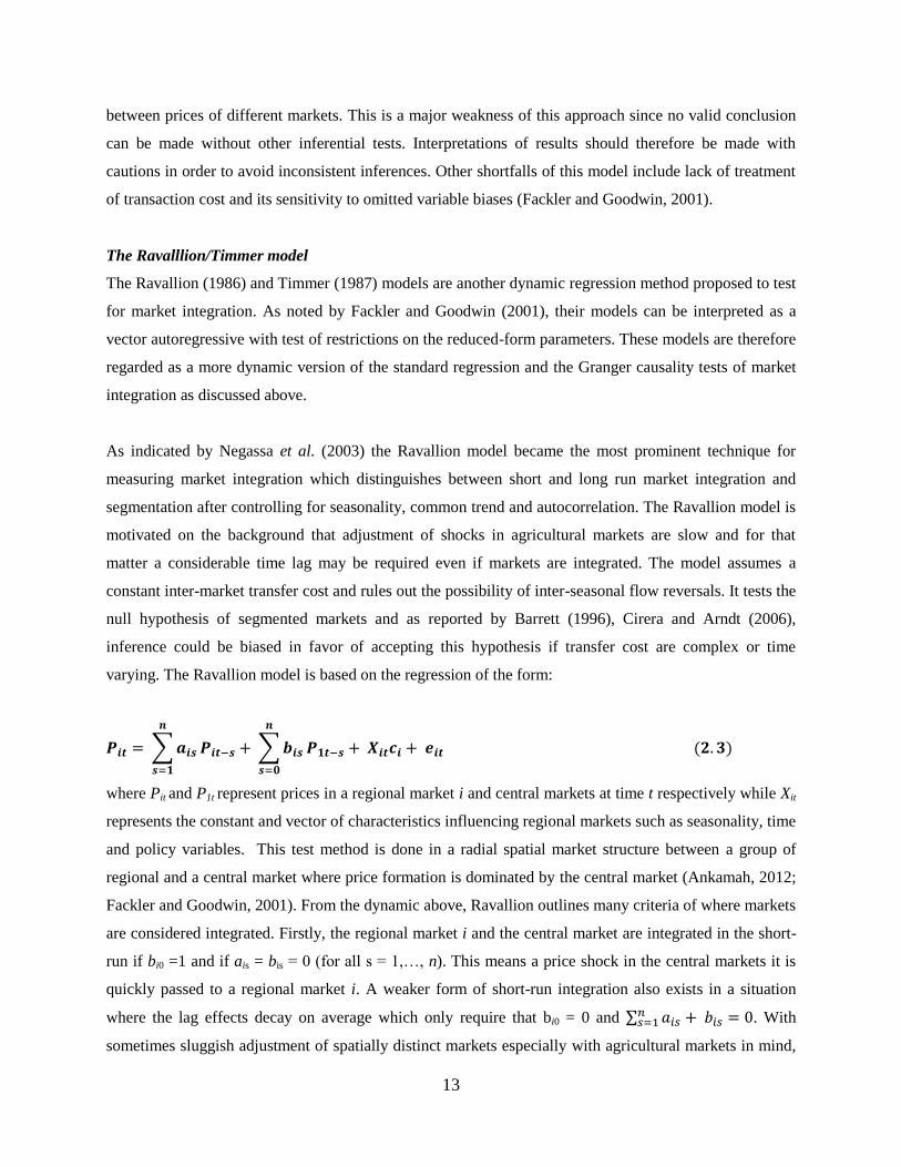
varying. The Ravallion model is based on the regression of the form:

𝑷𝒊𝒕 = ∑ 𝒂𝒊𝒔

𝒏

𝒔=𝟏

𝑷𝒊𝒕−𝒔 + ∑ 𝒃𝒊𝒔

𝒏

𝒔=𝟎

𝑷𝟏𝒕−𝒔 + 𝑿𝒊𝒕𝒄𝒊 + 𝒆𝒊𝒕 (𝟐. 𝟑)

where Pit and P1t represent prices in a regional market i and central markets at time t respectively while Xit

represents the constant and vector of characteristics influencing regional markets such as seasonality, time

and policy variables. This test method is done in a radial spatial market structure between a group of

regional and a central market where price formation is dominated by the central market (Ankamah, 2012;

Fackler and Goodwin, 2001). From the dynamic above, Ravallion outlines many criteria of where markets

are considered integrated. Firstly, the regional market i and the central market are integrated in the short-

run if bi0 =1 and if ais = bis = 0 (for all s = 1,…, n). This means a price shock in the central markets it is

quickly passed to a regional market i. A weaker form of short-run integration also exists in a situation

where the lag effects decay on average which only require that bi0 = 0 and ∑ 𝑎𝑖𝑠𝑛𝑠=1 + 𝑏𝑖𝑠 = 0. With

sometimes sluggish adjustment of spatially distinct markets especially with agricultural markets in mind,

14

Ravallion also proposed a test for long-run market equilibrium which requires that the condition

∑ 𝑎𝑖𝑠𝑛𝑠=1 + ∑ 𝑏𝑖𝑠

𝑛𝑠=0 = 1 is satisfied. This means a price shock in the central market takes a longer time

period to be transmitted to the regional markets i. A short-run integrated markets therefore implies long-

run integration but not the vice versa as can be seen from the conditions stated above.

A test of market isolations is also proposed by Ravallion where prices are expected to be equal to the

autarky prices (ai in the regression above).

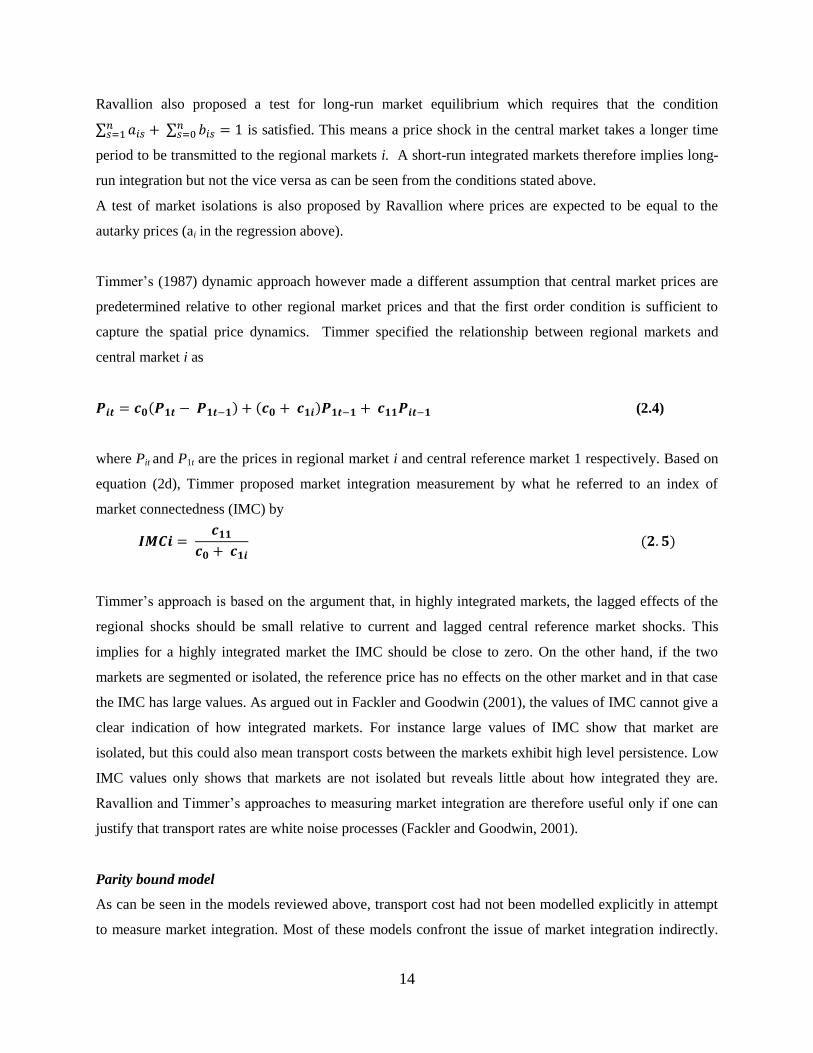
Timmer’s (1987) dynamic approach however made a different assumption that central market prices are

predetermined relative to other regional market prices and that the first order condition is sufficient to

capture the spatial price dynamics. Timmer specified the relationship between regional markets and

central market i as

𝑷𝒊𝒕 = 𝒄𝟎(𝑷𝟏𝒕 − 𝑷𝟏𝒕−𝟏) + (𝒄𝟎 + 𝒄𝟏𝒊)𝑷𝟏𝒕−𝟏 + 𝒄𝟏𝟏𝑷𝒊𝒕−𝟏 (2.4)

where Pit and P1t are the prices in regional market i and central reference market 1 respectively. Based on

equation (2d), Timmer proposed market integration measurement by what he referred to an index of

market connectedness (IMC) by

𝑰𝑴𝑪𝒊 = 𝒄𝟏𝟏

𝒄𝟎 + 𝒄𝟏𝒊 (𝟐. 𝟓)

Timmer’s approach is based on the argument that, in highly integrated markets, the lagged effects of the

regional shocks should be small relative to current and lagged central reference market shocks. This

implies for a highly integrated market the IMC should be close to zero. On the other hand, if the two

markets are segmented or isolated, the reference price has no effects on the other market and in that case

the IMC has large values. As argued out in Fackler and Goodwin (2001), the values of IMC cannot give a

clear indication of how integrated markets. For instance large values of IMC show that market are

isolated, but this could also mean transport costs between the markets exhibit high level persistence. Low

IMC values only shows that markets are not isolated but reveals little about how integrated they are.

Ravallion and Timmer’s approaches to measuring market integration are therefore useful only if one can

justify that transport rates are white noise processes (Fackler and Goodwin, 2001).

Parity bound model

As can be seen in the models reviewed above, transport cost had not been modelled explicitly in attempt

to measure market integration. Most of these models confront the issue of market integration indirectly.

15

Rather than examining transportation systems, interviewing tracking shipments and looking for

unexploited arbitrage, most researchers use time series econometrics applied to observed food prices

(Baulch, 1997). The parity bound model developed in studies of Spiller and Haung (1986), spiller and

wood (1996) and consequently used by Baulch (1997), Barrett and Li (2002) is one that attempts to

address the problem of transfer cost. The parity bound model therefore tries to utilize all available market

data i.e. prices, transfer cost, trade flows and volumes in its implementation.

The parity bound model (PBM), uses explicit information on transfer cost together with other market data

to assess efficiency of inter-regional markets. The model assumes that transfer cost plays a critical role in

determining price efficiency bounds (parity bound). The transfer costs determine the parity bounds within

which prices of a homogenous commodity in two geographically distinct markets can vary independently.

It is then expected that trade will cause prices in two markets to move on one for one basis when transfer

costs equal the inter-market price differential and there are no impediments to trade between the markets

(Baulch, 1997). This means spatial arbitrage conditions are binding. Trade will however, not occur when

the inter-market price differential is lower than the transfer cost. In this case the arbitrage condition will

not be binding which means lack of market integration.

The PBM therefore tries to assess the extent of market integration by distinguishing among three possible

trade regimes: regime I at the parity bounds in which spatial price differentials exactly equal the transfer

cost; regime II inside the parity bound s in which price differentials are less than transfer costs and finally

regime III outside the parity bounds in which price differentials exceed the transfer cost (Baulch, 1996).

The aim of the model is therefore to determine the probability of an observation falling under any of the

three regimes. This means it starts with the determination of the lower and the upper parity bounds for

which the spatial arbitrage condition occurs between the markets being considered. Establishing this

parity bounds is therefore a key requirement in the PBM and since transfer costs rarely exist, the task

could be quite complicated (Barrett, 1996). The PBM therefore relies on exogenous transaction data to

estimate the probability of achieving inter-market arbitrage conditions. The use of maximum likelihood

based estimators is noted to cope well with trade discontinuities and time varying transaction costs as

reported by Barrett (1996).

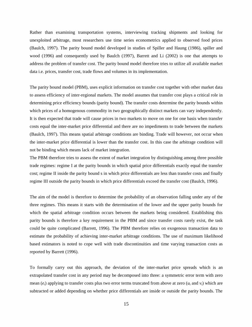
To formally carry out this approach, the deviation of the inter-market price spreads which is an

extrapolated transfer cost in any period may be decomposed into three: a symmetric error term with zero

mean (et) applying to transfer costs plus two error terms truncated from above at zero (ut and vt) which are

subtracted or added depending on whether price differentials are inside or outside the parity bounds. The

16

first error term et, allows transfer costs to vary between two period in response to seasonality or other

changes that occur through changes in the transport sector. The error term ut captures the extent to which

price differentials fall short of the parity bounds when there is no incentive to trade while the error term vt

measures how much price differentials exceed transfer cost which arbitrage conditions are violated. The

likelihood function for the PDM utilizing results derived by Weinston for the density of a normal plus

half normal distribution as specified by Baulch (1997) is:

𝑳 = ∏[𝜽𝟏𝒇𝒕𝟏 + 𝜽𝟐𝒇𝒕

𝟐 + (𝟏 − 𝜽𝟏 − 𝜽𝟐)𝒇𝒕𝟑]

𝑻

𝒕=𝟏

(𝟐. 𝟔)

where regime I : at the parity bounds

𝑓𝑡1 =

1

𝜎𝑒∅ [

𝑌𝑡 − 𝐾𝑡

𝜎𝑒] (2.6𝑎)

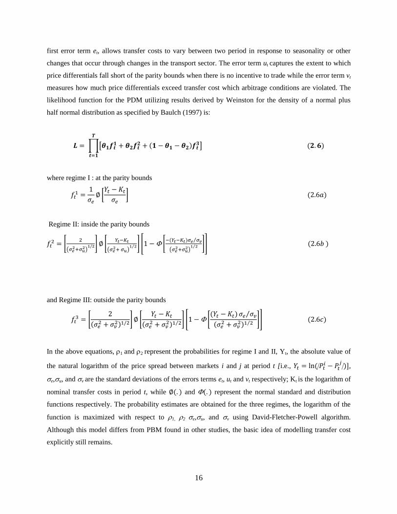
Regime II: inside the parity bounds

𝑓𝑡2 = [

2

(𝜎𝑒2+𝜎𝑢

2)1/2] ∅ [

𝑌𝑡−𝐾𝑡

(𝜎𝑒2+ 𝜎𝑢)

1 2⁄ ] [1 − [−(𝑌𝑡−𝐾𝑡)𝜎𝑒 𝜎𝑣⁄

(𝜎𝑒2+𝜎𝑢

2)1 2⁄ ]] (2.6𝑏 )

and Regime III: outside the parity bounds

𝑓𝑡3 = [

2

(𝜎𝑒2 + 𝜎𝑣

2)1/2] ∅ [

𝑌𝑡 − 𝐾𝑡

(𝜎𝑒2 + 𝜎𝑣

2)1 2⁄] [1 − [

(𝑌𝑡 − 𝐾𝑡) 𝜎𝑒 𝜎𝑣⁄

(𝜎𝑒2 + 𝜎𝑣

2)1 2⁄]] (2.6𝑐)

In the above equations, 1 and 2 represent the probabilities for regime I and II, Yt, the absolute value of

the natural logarithm of the price spread between markets i and j at period t [i.e., 𝑌𝑡 = ln (𝑃𝑡𝑖 − 𝑃𝑡

𝑗)],

e,u, and v are the standard deviations of the errors terms et, ut and vt respectively; Kt is the logarithm of

nominal transfer costs in period t, while ∅(. ) and (. ) represent the normal standard and distribution

functions respectively. The probability estimates are obtained for the three regimes, the logarithm of the

function is maximized with respect to 1, 2 e,u, and v using David-Fletcher-Powell algorithm.

Although this model differs from PBM found in other studies, the basic idea of modelling transfer cost

explicitly still remains.

17

The weakness of the PBM model becomes obvious considering the fact that transaction costs embody

several unobservable components which may be difficult to capture. This makes studies including data on

transfer costs quite tricky since some hidden components of transfer cost may be difficult obtain. The

PBM also does not give causes of why markets are integrated or not, it shows only that spatial arbitrage

condition are obeyed or violated (Barrett, 1996).

Impulse response analysis

The bound model is another dynamic technique that has been used to analyze market integration. It

involves application of exogenous shocks to variables in terms of a moving average representation of

Variable Autocorrelation (VAR) systems. In most market integration studies, causality tests are

inappropriate as pointed out by Rahman and Shahbaz, (2013). This is because, such tests fail to indicate

how much feedback exists from one variable to the other beyond the time period considered. To interpret

the implications of the models for patterns of price transmissions, causality and adjustments therefore

require consideration of the time path of prices after exogenous shock (Vavra and Goodwin, 2005).

The Impulse response function traces the effect of one standard deviation or one unit shock to one of the

variables on current and future values of all endogenous variables in a system over time and horizon

(Rahman and Shahbaz, 2013). Impulse response functions, expresses prices of regional markets as

function of current and lagged shocks (impulse). Studies that use this approach in analysis of market

integration argue it makes richer inferences in terms the dynamics of price adjustment compared to the

standard regression analyses since it evaluates dynamic time path of responses to market shocks

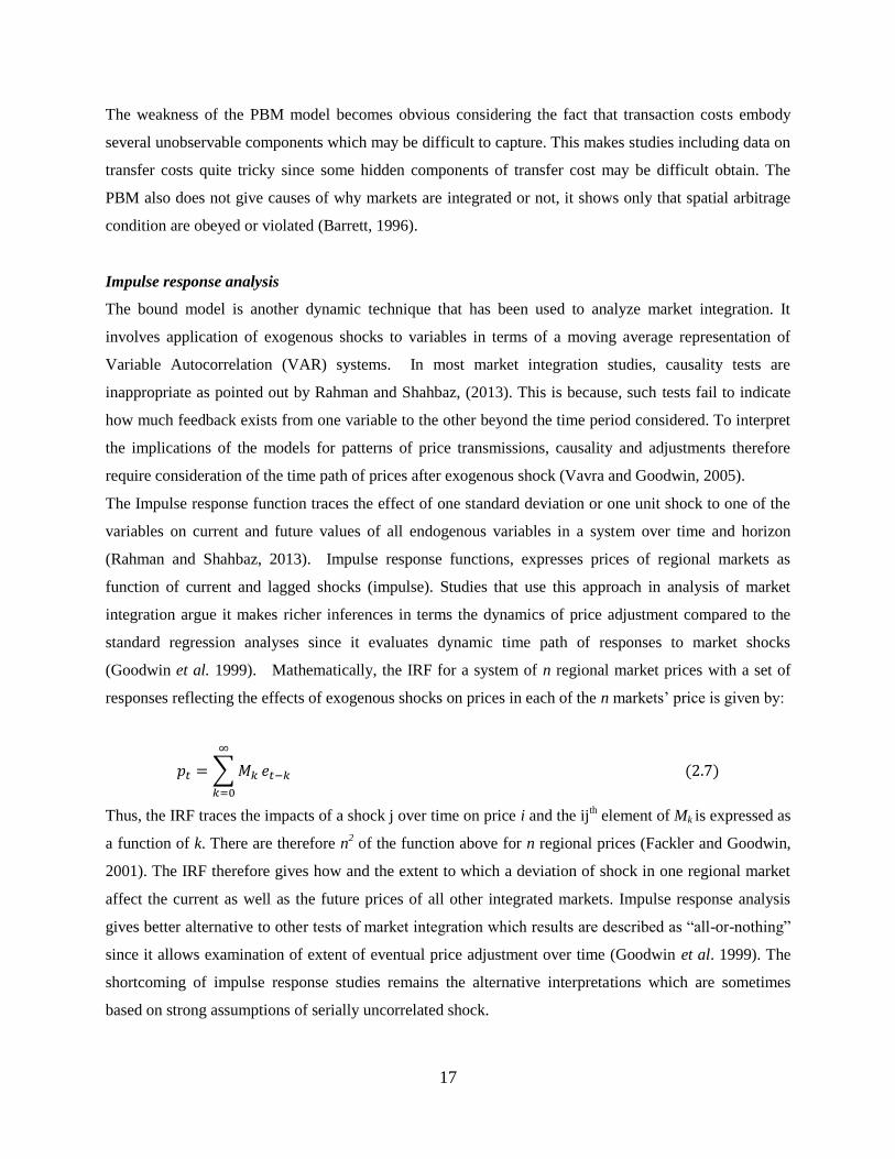
(Goodwin et al. 1999). Mathematically, the IRF for a system of n regional market prices with a set of

responses reflecting the effects of exogenous shocks on prices in each of the n markets’ price is given by:

𝑝𝑡 = ∑ 𝑀𝑘

∞

𝑘=0

𝑒𝑡−𝑘 (2.7)

Thus, the IRF traces the impacts of a shock j over time on price i and the ijth element of Mk is expressed as

a function of k. There are therefore n2 of the function above for n regional prices (Fackler and Goodwin,

2001). The IRF therefore gives how and the extent to which a deviation of shock in one regional market

affect the current as well as the future prices of all other integrated markets. Impulse response analysis

gives better alternative to other tests of market integration which results are described as “all-or-nothing”

since it allows examination of extent of eventual price adjustment over time (Goodwin et al. 1999). The

shortcoming of impulse response studies remains the alternative interpretations which are sometimes

based on strong assumptions of serially uncorrelated shock.

18

Cointegration model

The concept of co-integration for testing market has been used extensively in present studies following its

introduction by Engle and Granger (1987) and Engle and Yoo (1987). This approach is more useful

because most price series, especially nominal ones, used in the studies of market integration turn to

behave as nonstationary. This renders most of the conventional tests for market integration particularly,

those using simple regression invalid since the standard errors from such studies maybe inconsistent.

Recent studies have therefore made significant advances in attempt to solve such problems by exploring

current advances in econometrics. Cointegration in econometrics basically means different price series

have long-run relation. The idea helps to analyze the relationship that exists between two spatial markets

using price series from each market. Lack of cointegration between market price series is taken as market

segmentation or isolation. The Cointegration test of market integration is done through determination of

the order of integration of price series using unit root tests. A cointegration regression is then constructed

when prices are found to be integrated of the same order and then testing the stationarity of the residuals

from the cointegration regression. The cointegration test of market integration therefore involves

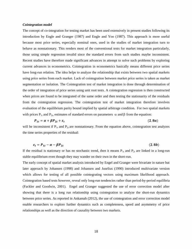
evaluation of the equilibrium parity bound implied by spatial arbitrage condition. For two spatial markets

with prices P1t and P2t, estimates of standard errors on parameters and from the equation:

𝑷𝟏𝒕 = 𝜶 + 𝜷𝑷𝟐𝒕 + 𝜺𝒕 (𝟐. 𝟖𝒂)

will be inconsistent if P1t and P2t are nonstationary. From the equation above, cointegration test analyzes

the time series properties of the residual:

𝜺𝒕 = 𝑷𝟏𝒕 − 𝜶 − 𝜷𝑷𝟐𝒕 (𝟐. 𝟖𝒃)

If the residual is stationary or has no stochastic trend, then it means P1t and P2t are linked in a long-run

stable equilibrium even though they may wander on their own in the short-run.

The early concept of spatial market analysis introduced by Engel and Granger were bivariate in nature but

later approach by Johansen (1998) and Johansen and Juselius (1990) introduced multivariate version

which allows for testing of all possible cointegrating vectors using maximum likelihood approach.

Cointegration based tests however, reveal only long-run tendencies rather than period-by-period equilibria

(Fackler and Goodwin, 2001). Engel and Granger suggested the use of error correction model after

showing that there is a long run relationship using cointegration to analyze the short-run dynamics

between price series. As reported in Ankamah (2012), the use of cointegration and error correction model

enable researchers to explore further dynamics such as completeness, speed and asymmetry of price

relationships as well as the direction of causality between two markets.

19

The use of cointegration test makes implicit assumption that transport costs are stationary or proportional

to prices in case of logarithmic transformations. This is sometimes regarded as a weakness because if

transport costs are non-stationary, then prices that are not integrated may not represent spatial arbitrage in

any case. Thus, as indicated by Barrett (1996) and Negassa et al. (2003) it may be completely consistent

with market integration even though one fails to find cointegration between two market price series if

transaction costs are non-stationary. Cointegration test alone is not sufficient to draw any meaningful

conclusion on market integration since the magnitude of cointegration coefficient may be far from unity, a

basic intuition behind market integration. The strength of the model remains its ability to allow for

consistent inferences in situations where individual market prices are non-stationary.

Switching regime (threshold autoregressive) models

The use of dynamic regression models in the test of market integration lack clearly articulated alternative

to the null hypothesis that market are integrated as argued by Fackler and Goodwin (2001). This

according to the authors is a problem when markets are imperfectly integrated because the network of

trading linkages may be changing over time due to factors such as seasonality. The switching regime

regression model is therefore designed to take care of such changes.

The model designed by Spiller and Wood (1998) suggest three possible regimes between two-location

markets M1 and M2: regime I where M1 ships to M2; regime II where and M2 ships to M1 and regime III

where there is trade between the two markets. The direction of trade depends on the transport rate from

one market to the other with positive supply region having the less net transport rate. Trade will however

not occur when there is equality in the transport rates involved in shipping from M1 to M2 and from M2 to

M1. The model provides estimate of probability of being in each regime conditional on the size of

observed price spread both ex ante and ex post. Integration between the two markets is tested with the

hypothesis that a particular regime’s probability equals one and all the others are zero. The Switching

regime model therefore uses price spreads as an indicator of market connectedness which maybe be

wrong since two markets may be connected simply because they both have a common trading partner.

Threshold Autoregressive (TAR) is a variation of the switching regime model used by Obstfeld and

Taylor (1997). In the TAR, a fixed but unknown transport cost is assumed to act as a threshold beyond

which price adjustment will take place and hence lead to market integration. When the price spread

exceeds the threshold, it reverse toward the threshold and when it is within the transaction cost band, it is

taken to behave in a serially independent ways (Fackler and Goodwin, 2001). This study approach

therefore recognizes the important role of transaction cost which are not dealt with in many models

20

reviewed above. However, as noted by Abdulai (2007), the assumption of fixed transaction cost which

implies fixed neutral band over the period under study could be too strong and hence a weakness of the

this model.

2.3 Review of similar studies

Analyses of market integration or market efficiency especially in the cereal sector have not been short in

literature over the years in Ghana. The first of such studies are those carried out by Alderman (`1992),

Shively (1996) and Badiane and Shively (1998). Alderman (1992) builds on the dynamic model used by

Ravallion (1986) described above to assess the efficiency of markets by investigating how information

flows across commodities. This study investigates the flow of information within a single market and then

the relationships between prices in other spatially distant markets. The aim of the study was to find out

whether prices of different agricultural commodities in Ghana are linked. In that case, policies could

concentrate on a single commodity’s price to achieve a broad base target in all other food commodities

especially, grains which are much consumed in Ghana. Alderman (1992) used maize as his reference

commodity and found that maize price movements are fully transmitted to other grains with three months

lags. He shows that in the long-run markets are integrated but his investigations reveal imperfections with

how markets process information. The possible explanation for lack of efficiency in terms of information

processing was given as, action of traders who may set prices of other grains in response to information

about maize prices which may require supply changes to bring the market to equilibrium. Another

explanation given was that some traders may not be dealing with all the grains considered and for that

matter, the cost of getting information may differ for different traders. His dynamic model therefore

realized that the grain market in Ghana was properly functioning but however lacks perfect information

flow in the marketing system.

This is however a reasonable finding considering the time the study was carried out, where Ghana’s

structural adjustment was still at its infant stages and communication technology such as mobile phones

and internet were nearly non-existent. Although our study looks at the root crop markets, it does not look

at intercommodity price transmission. The current penetration of Information Communication

Technology (ICT) tools are also expected to make information less difficult to access and hence improve

the imperfection regarding information processing

Shively (1996) is another study which looks at behavior of food commodity market prices in Ghana.

Shively used an Autoregressive Conditional Heteroskedasticity (ARCH) regression analysis to investigate

variability of monthly wholesale prices of maize in two markets in Ghana. Although this study differs in

terms of the motivation behind, it gives important information on how volatile maize prices are and helps

21

to understand how production, storage and trade influence changes in prices. This gives an idea of how

commodities prices have been formed as well as the dynamics of price variation in the Ghanaian markets

after structural adjustment which involved market liberalization, fiscal austerity and monetary reforms.

His results show that prices of maize were more variable and higher in the years when economic reforms

were adopted compared to years before and after. The results also suggest that the variations of prices are

different in the different markets considered. For instance the years subsequent to the economic reforms

saw Bolgatanga market’s price volatility reduced compared to the Cape Coast market. Reduction in price

volatility was attributed to storage during the reforms and possibly trade with the southern part of Burkina

Faso. Again, this brings into mind the role of trade on prices as we see Ghana export yam.

Badiane and Shively (1998) build on the earlier spatial studies above and investigate the roles played by

market integration and transport costs in explaining changes in prices in Ghana. This study examines both

theoretically and empirically, how price formation is influenced by transport costs and market integration

using a dynamic model. They argue that the link between prices and stockholding behavior provides a

mechanism for both intertemporal and spatial arbitrage and for that matter central market price history

could explain price levels in hinterland markets. In analyzing the market integration, the authors used the

Ravallion (1986) approach above. Their model investigated the relationship between local and a central

market of maize in the short-run and long-run. They defined the central market as the net exporting

market whereas local markets represent the net importing markets. The authors investigated the link

between market integration and price volatility by regressing the variance of local market price on central

market price history. This was based on the model by Deaton and Laroque (1992) which shows that the

link between prices and stockholding behavior creates a link between current period price volatility and

past prices. Thus, the current price in a local market is believed to depend on its previous price, central

market prices and harvest if there is positive storage and the markets are believed to be connected. Given

an initial price shock in the central market, Badiane and Shively (1998) developed a dynamic price

adjustment equation to compute the effects of this initial shocks originating from the central market on

outlying markets. Using maize wholesale prices covering the period of 1980-1993, they showed that the

price adjustment process in a particular market is determined by the degree of its interdependence on the

central market where the shock originates.

The price reductions in various local markets in Ghana following the 1983 economic reforms were

therefore attributed forces arising from both the local and the central markets. They however,

acknowledge the important role of transport cost in both the speed of the adjustment and the degree of

market connectedness and pointed out that changes in transport cost can be expected to lead to a different

22

pattern of responses of local markets to central market’s price shock. The path of a local market’s price at

a particular period after initial shock in a central market was consequently expressed as a function of the

long-run multiplier between local/central market pairs, changes in the transport cost, prices in the local

market prior to shocks in the central market and local market price level after shock has been fully

transmitted to the local market. Thus, local prices also respond to transport cost as they adjust to volumes

traded between two market pairs. In summary, Badiane and Shively (1988) produced results which

confirm Alderman (1992) that the Ghanaian maize markets are fairly well integrated with strong

connection between Techiman-Makola market pairs than the Techiman-Bolgatanga. Yet, time required

for price shocks to be transmitted between both market pairs are the same. There was a weak link in terms

contribution of price fall in the Bolgatanga market arising from a price fall in the central market, the

Techiman. Thus, prices in local markets are determined primarily on their own past values and other local

factors but not the central market’s price due to poor integration between markets. The importance of

market integration in price transmission was shown with evidence from the Makola market which is well

connected with the Techiman market and shows strong responses. The authors also used simulation to

show the importance of transport cost in determining how sensitive local market prices are to central

market by increasing the estimated transport cost. The results show that large transport costs dampen the

effect of the central market’s price shocks on local prices. This study has been examined extensively

because it does not only look at market integration but also how the integration affects price formation in

local markets. It also deals with the issue of transport cost which much spatial price literature are silent

on. It therefore gives important background to this study and helps to understand why some of the results

may be obtained particularly, with yam which transport costs cannot be overlooked in its marketing

process.

Following these early studies on spatial prices in Ghana, several authors have looked at different

commodities or markets and found interesting results. Abdulai (2000) used a cointegration test that allows

for symmetric price adjustment towards long-run equilibrium relationships to examine linkages between

principal maize markets in Ghana. His approach differs from the previous studies in that, he assumes

economic agents act to restore equilibrium when deviation from equilibrium exceeds a critical threshold

in which case the benefit of the adjustment exceeds the cost. Also his study disagrees that price responses

are always symmetric .This implies that a shock from a central market will elicit similar response in local

markets, but is of the view that certain features associated with market imperfections may lead to

asymmetric responses. He argues that effort of market participants to exploit arbitrage opportunities can

result in the maintenance of equilibrium relationships among commodity prices in distant markets.

Abdulai (2000) therefore employed threshold cointegration analysis models developed by Enders and

23

Granger (1998) to examine the relationships between wholesale prices of maize in Techiman (central

market) and two local markets (Accra and Bolgatanga) with the objective of determining whether

transmission between these markets is symmetric or asymmetric. The study results show that local

markets response to central market prices is asymmetric in the sense that the response to falling central

market prices is not the same as the response to increasing central market prices. For instance his results

show that while prices in the Accra market adjust to eliminate about 40% of a unit negative change in the

deviation from the equilibrium relationship created by the Techiman market, it adjust to eliminate only

13% of a unit positive change in the central market. In other words, increase in maize prices in the

Techiman market is quickly passed to the Accra market while a decrease takes longer time to be passed to

the Accra market. Again the study focuses on the grain sector as well as using the Techiman market as its

central market. The root and tuber crops which form part of major staples however, remain less studied

and this makes our study an important one by filling the gap between the extensively studied grain sector

and the root and tuber sector which provide food security for many households in Ghana.

In further studies about the grain sector, Ankamah (2012) used regional monthly prices of maize from

2002 to 2010 to assess the linkages between regional markets in Ghana. Using the threshold

autoregressive model, he shows that regional markets of maize are integrated, but characterized by

asymmetry in terms of the price adjustment. His results also show that there is either a bidirectional

market interdependence or causality to price changes in both the short-run and long-run. There is

however, heterogeneity in terms of responses towards positive and negative deviations in the long run.

The adjustment processes of all markets were not the same. For instance, whiles adjustment between the

Greater Accra-Brong Ahafo market pair exhibited positive asymmetry, the adjustment between of the

Brong Ahafo and the Northern, Ashanti, and Central regional markets exhibited negative asymmetry. The

study also found the time required for adjustment after a shock in the central market to be ranging from 7

months to 26 months with the adjustments between Greater Accra and the Brong Ahafo markets requiring

the least time. The author attributed the integration of regional markets to improvement in communication

infrastructures which allows for easy access to information by market agents.

The improvement in communication infrastructure raised here has been noted to play a very important

role in market integration. A similar study by Chowa (2014) in the Malawian maize markets shows that

ICT based market interventions have positively influenced market integration and price transmission.

They asserted that modern ICT tools have contributed to the reduction in information search cost leading

to complete market efficiency in Malawi. Nevertheless, earlier studies (Alderman, 1992; Shively, 1996;

Badiane and Shively 1998) have found similar results in the maize market in Ghana when there was low

ICT development. Studies with different commodities other than the maize are needed to understand

24

whether improvement in communication infrastructures have aided integration of all commodity markets

or just some selected commodities.

In a more recent study, Adom (2014) examined spatial market integration of domestically imported rice

markets and the extent of substitution between locally produced rice and imported rice. Based on current

monthly wholesale prices from January 2006 to December 2013, the author used Johansen multivariate

and cointegration models to show that the foreign rice markets in Ghana are well integrated, although

there are some imperfections, indicating that foreign rice market in Ghana provides opportunities for

arbitrage condition. He discovered the Accra market as the dominant market leader among the markets

considered. His analysis of the effect of government policies during the 2007/2008 periods reveals that

the policies somewhat succeeded in moderating the price fluctuations during the period, even though

various local markets differed in their responses to central market price shocks. The results of regional

substitution between the imported rice and the local rice suggest that there are evidences to that effect in

the long-run but no clear evidence in the short-run indicating that the two products are not perfect

substitutes. Hence, the author believes that government policy to limit importation of foreign rice in order

to raise producer prices of locally produced rice will only have a mild effect on producers but slam a

heavy burden on household’s budget.

In another spatial price analysis studies in Ghana, Amikuzuno (2010) used Johansen’s estimation method

to analyze the seasonal asymmetric price transmission in the Ghanaian tomato market. The tomato market

in Ghana shows significant seasonal patterns due to weekly price variations as noted by the study. The

author analyzed the dynamics and interdependence of wholesale prices of five major markets: Accra,

Kumasi, Techiman, Tamale, and Navrongo. Using semi-monthly data from March 2007 to February 2010

in a multivariate form of the Johansen’s estimation procedure, the author found strong evidence of market

integration with fast price transmission between markets. The study also found that any shock to the

tomato market equilibrium also triggers responses from the production regions which are the Tamale and

the Navrongo markets. The transmission of tomato price shocks were found to exhibit regime-dependent

adjustment with generally strong error-correction rates ranging from 10% to more than 40% per each

three days. This study gives important dimension to price transmission of highly perishable commodities

which are difficult to store. It also gives important dimension to the frequency of data which are required

for spatial prices. Although yam is different in terms of their features, their perishable natures make this

study interesting to compare with Amikuzuno (2010). As highlighted by Meyer and von Cramon-

Taubadel (2004), perishability plays a role in causing asymmetry in price transmission of products. They

think traders might hesitate to raise prices for perishable products for fear of spoilage which would lead to

25

negative asymmetry. However, Heien (1980) has rather opposite view that changing prices is more of

problem for products with longer shelf life rather than perishables since price change for the former

brings about higher cost and loss of goodwill. This study will contribute to such line of reasoning.

In a similar study, Mensah Bonsu et al. (2011) used the Johansen’s cointegration approach to analyze the

efficiency of plantain market system. They categorized the plantain markets in Ghana into central

consumption, assembling and producing markets and shows that arbitrage in the plantain marketing

system is working. Thus, there were both short-run and long-run relationships between the central market

(Accra), the assembling markets (Kumasi, Koforidua, and Sunyani) and the production markets (Goaso,

Begoro and Obogo). However, they realized the speed of price transmission between the central market

and the assembling and production markets was relatively weak at 27.7% compared to the 100%

threshold. Hence, they suggested the need for improvement in the market information in production areas.

With significant penetration of mobiles phones which Egyir et al. (2011) noted as facilitating speedy

transmission of market information, continuous studies are required to assess how the speed of

transmission has evolved in various commodity markets. This study aims to throw more light on the

matter.

Narrowing down on the root and tuber sectors, it is realized that not much has been done in terms of

spatial price analysis. This is because less attention has been given to the sector due to less trading

activity unlike the cereal sector. However, Acquah et al. (2012) analyzed price transmission in the

cassava market in Ghana using the Johansen cointegration, Granger causality and autoregressive

distributed lag models. They used weekly prices from 2008 to 2010 for six major markets in Ghana. They

showed that the price series of cassava markets were integrated of order one which means that there is a

unit root for market prices of cassava. They realized that there are no long-run relationships between

market prices of cassava. This shows there is poor price transmission between the different cassava

markets considered. There was also no causality between the reference market (Techiman) and the other

markets showing independence of the various markets. However, their results are not surprising because

cassava is not much traded in Ghana due to its low value-to-volume ratio. The costs of transportation are

therefore high which limits trade between regions. Comparing cassava and yam, the latter is much traded

and even exported. This study seeks to add to the sector’s investigation of market efficiency.

Away from Ghana, spatially price studies have been carried out in different regions including intra-

regional and inter-regional studies. To highlight a few studies, Muyatwa (2001) used the cointegration

analysis and the error correction models to examine the integration of regional markets in Zambia

26

following the liberalization of the maize markets. Using monthly wholesale prices from 1993 to 1997, the

study found that both the magnitude and speed of price transmission between regional markets are much

limited. The results also show that even though there has been rapid emergence of the private sector, the

rate at which they are filling the gap left by the state has been slow due to various constraints such as lack

of access to information and poor transportation infrastructures. Using a different framework from

cointegration models, Negassa and Myers (2007) applied an extension of the parity bound model which

allows dynamic shifts in regime probabilities in response to marketing policy to study the maize and

wheat markets in Ethiopia. Their results show a dynamic adjustment path in the grain markets and, also

the grain marketing reforms have improved efficiency in some markets but worsened it in others. They

pointed out misallocation of resources in the two markets as the cause of inefficiency. They suggest

different policy responses for the two commodities to improve efficiency, since there were asymmetries

in terms of profit made by maize and wheat traders.

In more recent studies, Serebrennikov et al. (2014) examined the spatial integration of the Russian

domestic wheat markets. Their study was based on the fact that the Russian Government always

intervened in the wheat market during periods of shortage in domestic supply. They therefore used the

threshold autoregressive model to understand whether the magnitude of transaction cost is high enough to

cause a break in the short-run linkages between the Russian wheat markets. Their results show that the

domestic markets became more active during restriction of export. In some cases, they found evidence of

trade between domestic markets even though transaction costs were higher than potential returns from

trade. They attributed this to other forces for instance, information flow which may determine trade

behaviors apart from the arbitrage condition. Mengel and von Cramon-Taubadel (2014) analyzed the

distance and border effects on price transmission of cereals which they believe are relatively more

homogenous in terms of marketable qualities. The authors therefore used the price transmission estimates

for 1189 cereal markets pairs from 57 studies to test the effects of border distance on price transmission

using meta-analysis. Their findings suggest that distance and border have effects on price transmission as

well as long-run price relationship between market pairs. Thus, both border and distance reduces

probability of price cointegration and consequently find that speed of price adjustment between

international markets is slower on the average than intra-national markets pairs.

2.4 Lessons and conclusion from review

There have been several models developed to empirically examine the behavior of spatial prices over the

past decades. They range from simple correlation tests to more sophisticated cointegration because of

27

recent advances in econometrics. Different tests make different assumptions and formulate different

hypothesis to achieve their objectives. Based on these assumptions and hypothesis, some of these tests

could lead to invalid conclusions. However, there is no single test which has been declared best among

these several models since each test has its limitations and strengths. Many of these limitations have been

pointed out above but one serious concern with most of these tests has been the assumption made about

transaction costs. It can be seen that most of these tests do not explicitly consider transaction costs. Few

of the models which take into account the critical role of transaction costs, do so by assumption due to

lack of data and also the inability to capture the different components of transaction costs. It is therefore

necessary that one understands the institutional mechanism and dynamics of a particular market in order

to make meaningful interpretations of spatial tests. For instance as indicated by Fackler and Goodwin

(2001), knowledge of continuous flow of commodities between two markets, direction of commodity

flow and the pattern of seasonality could be very useful in interpretation of tests of market integration.

The various tests therefore provide information on simple relationships between prices and it is necessary

that results are interpreted in the context of more realistic and factual behavior of the markets under

consideration. In some case, a single test may not be enough, but aggregation of different tests could give

a better situation of market integration.

On empirical studies, the use of cointegration analysis seems to dominate current studies. Most studies

however augment results from this test with other inferential techniques such as the threshold

autoregressive model, the Granger causality tests and impulse responses in order to draw more concrete

conclusions.

About the study area, spatial price studies to assess efficiency of commodity markets have not been

lacking in Ghana just as in other countries. However, dynamic change in behaviors of market agents and

with improvement in technology and somewhat infrastructure means continuous assessment is required in

order to keep policy makers informed and updated. Most of the studies have also focused on the cereal

sector, especially maize and rice, leaving a gap between the cereal and the root crop sector. Also as noted

by many researchers (Shively 1996, Badiane and Shively 1998 and Amikuzuno 2010), Ghana’s economy

is one of the economies that has experienced trade liberalization both domestically and to some extent

internationally. This makes the various commodity markets worth studying in order to understand how

similar economies which have liberalized market system and major economic reforms in the region

evolved over the years.

28

Chapter 3- Research methodology

4.1 Study area and data collection

The study is carried out in Ghana which is made up of ten administrative regions out of which yam

production takes place in seven of them. Production is mainly in the Northern and Eastern part of the

country with distribution routes to consumption markets shown on the figure 3.1 below. Due to the

widespread of yam consumption in Ghana, there are different marketing centers which can be categorized

into production and consumption markets. The markets chosen for this study are the markets of Accra,

Kumasi, Techiman, Tamale and Wa. These markets are chosen based on the major marketing routes and

data availability. It can be seen that most of the marketing routes lead to the Accra market which is a main

consumption market. The Accra market also serves as the main center where exporters compete for yam

for export though recent competition has forced some exporters to go to other production and rural

markets. The Accra market is therefore chosen as the central market for this study with all other markets

analyzed in reference to this market.

Figure 3.1 Marketing routes of yam in Ghana. Source: Adopted from Anaadumba (2013)

The data for this study is obtained from Statistical Research and Information Directorate (SRID) of the

Ministry of Food and Agriculture (MoFA) in Ghana. The data is cross-checked with a similar set of data

Techiman

Kumasi

Techiman

Tamale

Techiman

Wa

Accra

29

from FAOSTAT to iron out differences that arise. This data are collected by District Agricultural

Development Units in Ghana on weekly basis. The weekly data are used to compute monthly prices by

taking the average of the weekly prices. One key consideration in market integration analysis is the

frequency of the data. As noted by Amikuzuno (2010), high frequency data such as weekly data are

believed to capture precisely price transmission mechanisms better than low frequency data. However, as

noted by Mensah-Bonsu et al. (2010), high frequency data such as weekly series are noted to have several

long-run periods in which prices are constant. This could invalidate the statistical assumption of

independent and identically distributed of the error term that follows a continuous distribution. Weekly

prices could also pose greater challenges due to several missing figures which must be interpolated. This

study therefore uses monthly wholesale prices from 2006 to 2013, a total of 96 observations for each

market. Markets with missing figures are interpolated with previous monthly averages. The Tamale and

Wa markets are located in the northern part of Ghana while Techiman and Kumasi markets are more

central. The Accra market is located in the southern part of the country. The locations of the selected

markets give a good spatial spread for this study. The prices are in nominal terms and the currency unit is

Ghana Cedi (GHC). The prices are recorded per 250kg units. In order to interpret the econometric results

in terms of elasticity or percentage change, the various price series are log-transformed during various

empirical analyses.

3.2 Analytical methods

The concept of market integration has been presently dealt with in a cointegration framework as has been

shown in the literature review section. The rationale behind the use of cointegration models is the fact that

different variables may wander around in the short round but possess long-run equilibrium relationships.

This means that the variables may move together in the long-run. The model is therefore used to achieve

the first objective of this study which seeks to determine relationships between prices of regional yam

markets in Ghana. The use of this method in market integration studies has been welcomed since most

economic series have been found to be non-stationary. The use of cointegration involves several

adjustments and tests processes of the data in order to ensure price series exhibit the right characteristics

such as stationarity. The analysis starts with a unit root test of each series in order to ensure series do not

exhibit random walk and in some cases with a drift. Estimating ordinary least square from data with

random walk could lead to spurious regression and this may invalidate the hypotheses being tested as

indicated by Granger and Newbold (1974). As indicated by Alemu and Van Schalkwyk (2008) price data

collected over several periods must be adjusted for seasonality in order to avoid inconsistent and

inaccurate results. This seasonality in price data could be stable or variable due to natural phenomena

30

such as weather or behavior of economic agents respectively. Seasonality could be deterministic where

similar trends are observed year after year, random or both (Hylleberg et al. 1990). Depending on the

type of seasonality observed, different filtering approaches are used in order to correct for the problem.

For instance if a series is found to be deterministic as mostly assumed by researchers, a seasonal dummy

can be introduced in the model. To take care of seasonality in the price data, this study employs the

HEGY seasonal unit root tests developed for quarterly data by Hylleberg et al. (1990) and later extended

by Beaulieu and Miron (1993) for monthly data. This framework of analyses allows for examination of

seasonal and non-seasonal unit root processes in the data. The null hypothesis of unit root at zero is tested

against the alternate of stationarity for the model:

∆𝟏𝟐𝒚𝒊𝒕 = 𝜷° + 𝜸𝒕 + ∑ 𝜷𝒊

𝟏𝟏

𝒊=𝟏

𝑫𝒊𝒕 + ∑ 𝝅𝒌𝒛𝒌,𝒕−𝟏

𝟏𝟐

𝒌=𝟏

+ ∑ 𝜹𝒋∆𝟏𝟐𝒚𝒊𝒕−𝒋

𝒑

𝒋=𝟏

+ 𝜺𝒊𝒕 (3.1)

where 𝛽0, 𝛽𝑖, 𝜋𝑘 and 𝛿𝑗 are parameters to be estimated. The 𝐷𝑖𝑡 is a seasonal dummy which is equal to 1

for month i and 0 if otherwise, 𝑡 is a trend variable, 𝑧𝑘,𝑡−1 are non-singular linear transformations of

lagged values of 𝑦𝑖𝑡, 휀𝑖𝑡 is the error term and 𝑝 is the lag value selected automatically with the Ackaike

Information Criteria (AIC). From the above equation, the null hypothesis involves testing 𝐻𝑘𝑜: 𝜋𝑘 = 0 for

k = 1, 2 as against the alternative of 𝐻𝑘1: 𝜋𝑘 < 0 using t-statistics. Also using F-statistics, the complex

unit root is tested with the joint null hypothesis 𝐻𝑘0: 𝜋𝑘−1 = 𝜋𝑘 = 0 for k = 4,6,8,10,12 as against the

alternative of 𝐻𝑘1: 𝜋𝑘−1 ≠ 0 𝑜𝑟 𝜋𝑘 ≠ 0. The above test is augmented with the Canova and Hanson (1995)

Lagrangian multiplier type which tests null hypothesis of stationarity, implying that the seasonal pattern is

deterministic against the alternative of seasonal unit root for the individual or joint frequencies. From

equation 3.2, the Canova and Hanson approach investigates the instability of the parameter 𝛽𝑖𝑡 by testing

𝛽𝑖𝑡 = 𝛽𝑖𝑡−1 + 휀𝑡 and 𝑉𝑎𝑟(𝜇𝑡) = 0. A rejection of the null hypothesis means seasonality in the data is not

constant. This implies the null hypothesis should not be rejected for this test after adjusting for seasonality

using seasonal dummy.

Based on the conclusion from this seasonality test, the data is adjusted with an appropriate treatment

method. The most common treatment or filtering method in case of non-constant seasonality is the

introduction of seasonal dummy but in case of deterministic seasonality, the OLS estimation is the same

whether the data is treated or not as noted by Brendstrup et al. (2001).

3.2.1 Test for Unit roots in the presence of structural breaks

After the seasonal adjustment the conventional unit root test, called the Augmented Dickey-Fuller (ADF)

test, is used to examine the price series in order to find out if they are stationary or possess unit roots. The

ADF regression for a deseasonalized series Pit (i=1,2,..) is

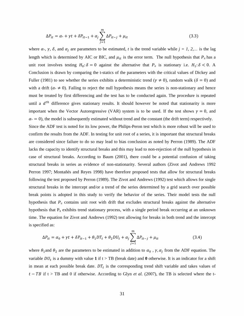
31

∆𝑃𝑖𝑡 = 𝛼° + 𝛾𝑡 + 𝛿𝑃𝑖𝑡−1 + 𝛼𝑗 ∑ ∆𝑃𝑖𝑡−𝑗

𝑚

𝑗=1

+ 𝜇𝑖𝑡 (3.3)

where 𝛼°, 𝛾, 𝛿, and 𝛼𝑗 are parameters to be estimated, t is the trend variable while j = 1, 2,… is the lag

length which is determined by AIC or BIC, and 𝜇𝑖𝑡 is the error term. The null hypothesis that Pit has a

unit root involves testing 𝐻0: 𝛿 = 0 against the alternative that Pit is stationary i.e. 𝐻1: 𝛿 < 0. A

Conclusion is drawn by comparing the t-statics of the parameters with the critical values of Dickey and

Fuller (1981) to see whether the series exhibits a deterministic trend (𝛾 ≠ 0), random walk (𝛿 = 0) and

with a drift (𝛼° ≠ 0). Failing to reject the null hypothesis means the series is non-stationary and hence

must be treated by first differencing and the test has to be conducted again. The procedure is repeated

until a 𝑑𝑡ℎ difference gives stationary results. It should however be noted that stationarity is more

important when the Vector Autoregressive (VAR) system is to be used. If the test shows 𝛾 = 0, and

𝛼° = 0), the model is subsequently estimated without trend and the constant (the drift term) respectively.

Since the ADF test is noted for its low power, the Philips-Peron test which is more robust will be used to

confirm the results from the ADF. In testing for unit root of a series, it is important that structural breaks

are considered since failure to do so may lead to bias conclusion as noted by Perron (1989). The ADF

lacks the capacity to identify structural breaks and this may lead to non-rejection of the null hypothesis in

case of structural breaks. According to Baum (2001), there could be a potential confusion of taking

structural breaks in series as evidence of non-stationarity. Several authors (Zivot and Andrews 1992

Perron 1997; Montañés and Reyes 1998) have therefore proposed tests that allow for structural breaks

following the test proposed by Perron (1989). The Zivot and Andrews (1992) test which allows for single

structural breaks in the intercept and/or a trend of the series determined by a grid search over possible

break points is adopted in this study to verify the behavior of the series. Their model tests the null

hypothesis that Pit contains unit root with drift that excludes structural breaks against the alternative

hypothesis that Pit exhibits trend stationary process, with a single period break occurring at an unknown

time. The equation for Zivot and Andrews (1992) test allowing for breaks in both trend and the intercept

is specified as:

∆𝑃𝑖𝑡 = 𝛼0 + 𝛾𝑡 + 𝛿𝑃𝑖𝑡−1 + 𝜃1𝐷𝑇𝑡 + 𝜃2𝐷𝑈𝑡 + 𝛼𝑗 ∑ ∆𝑃𝑖𝑡−𝑗

𝑚

𝑗=1

+ 𝜇𝑖𝑡 (3.4)

where 𝜃1and 𝜃2 are the parameters to be estimated in addition to 𝛼0 , 𝛾, 𝛼𝑗 from the ADF equation. The

variable 𝐷𝑈𝑡 is a dummy with value 1 if t > TB (break date) and 0 otherwise. It is an indicator for a shift

in mean at each possible break date. 𝐷𝑇𝑡 is the corresponding trend shift variable and takes values of

𝑡 − 𝑇𝐵 if t > TB and 0 if otherwise. According to Glyn et al. (2007), the TB is selected where the t-

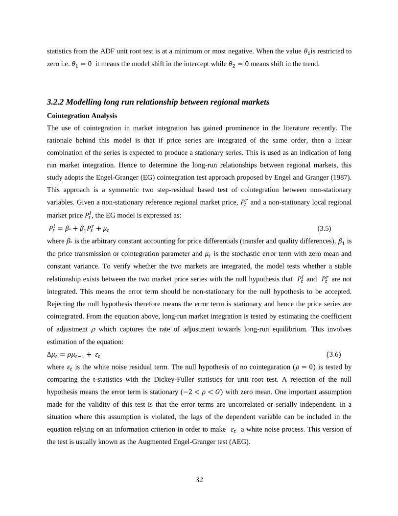
32

statistics from the ADF unit root test is at a minimum or most negative. When the value 𝜃1is restricted to

zero i.e. 𝜃1 = 0 it means the model shift in the intercept while 𝜃2 = 0 means shift in the trend.

3.2.2 Modelling long run relationship between regional markets

Cointegration Analysis

The use of cointegration in market integration has gained prominence in the literature recently. The

rationale behind this model is that if price series are integrated of the same order, then a linear

combination of the series is expected to produce a stationary series. This is used as an indication of long

run market integration. Hence to determine the long-run relationships between regional markets, this

study adopts the Engel-Granger (EG) cointegration test approach proposed by Engel and Granger (1987).

This approach is a symmetric two step-residual based test of cointegration between non-stationary

variables. Given a non-stationary reference regional market price, 𝑃𝑡𝑟 and a non-stationary local regional

market price 𝑃𝑡𝑙, the EG model is expressed as:

𝑃𝑡𝑙 = 𝛽° + 𝛽1𝑃𝑡

𝑟 + 𝜇𝑡 (3.5)

where 𝛽° is the arbitrary constant accounting for price differentials (transfer and quality differences), 𝛽1 is

the price transmission or cointegration parameter and 𝜇𝑡 is the stochastic error term with zero mean and

constant variance. To verify whether the two markets are integrated, the model tests whether a stable

relationship exists between the two market price series with the null hypothesis that 𝑃𝑡𝑙 and 𝑃𝑡

𝑟 are not

integrated. This means the error term should be non-stationary for the null hypothesis to be accepted.

Rejecting the null hypothesis therefore means the error term is stationary and hence the price series are

cointegrated. From the equation above, long-run market integration is tested by estimating the coefficient

of adjustment which captures the rate of adjustment towards long-run equilibrium. This involves

estimation of the equation:

∆𝜇𝑡 = 𝜌𝜇𝑡−1 + 휀𝑡 (3.6)

where 휀𝑡 is the white noise residual term. The null hypothesis of no cointegaration (𝜌 = 0) is tested by

comparing the t-statistics with the Dickey-Fuller statistics for unit root test. A rejection of the null

hypothesis means the error term is stationary (−2 < 𝜌 < 𝑂) with zero mean. One important assumption

made for the validity of this test is that the error terms are uncorrelated or serially independent. In a

situation where this assumption is violated, the lags of the dependent variable can be included in the

equation relying on an information criterion in order to make 휀𝑡 a white noise process. This version of

the test is usually known as the Augmented Engel-Granger test (AEG).

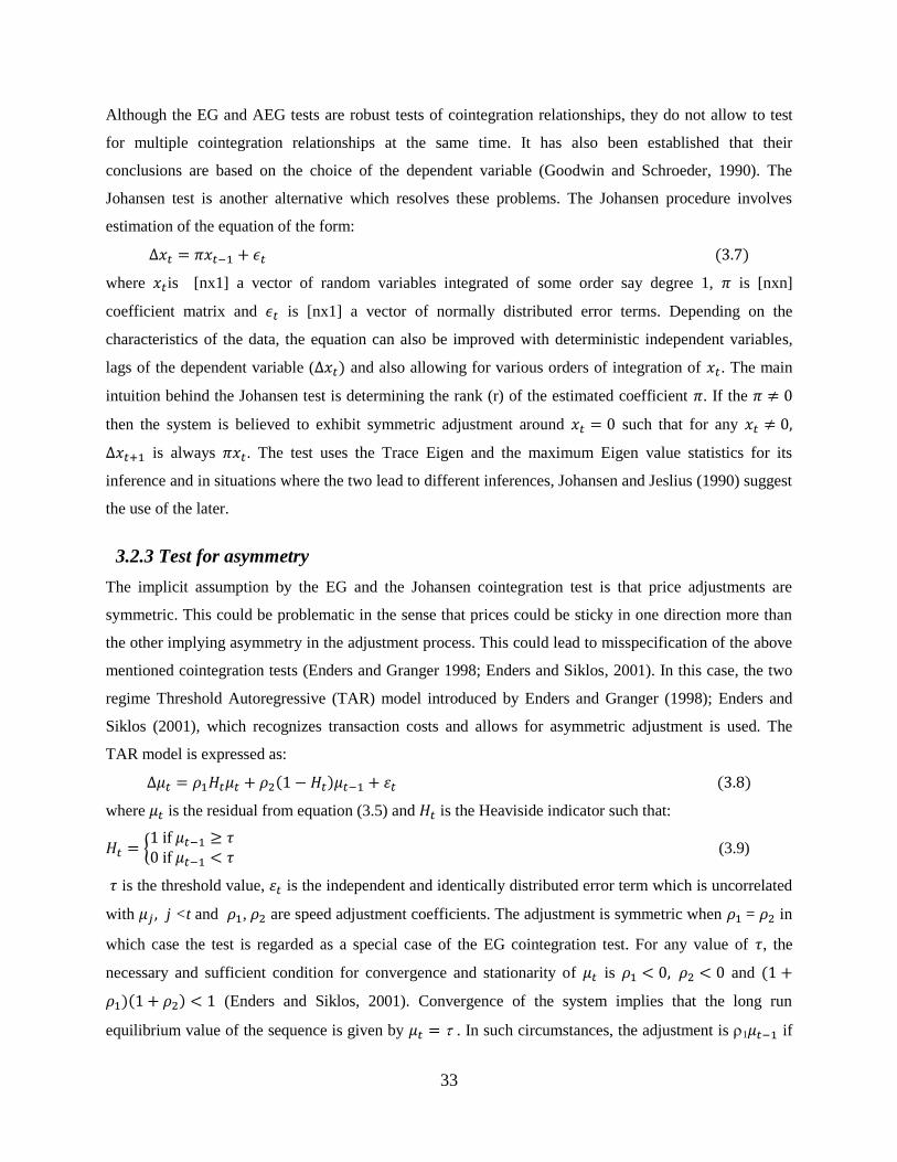
33

Although the EG and AEG tests are robust tests of cointegration relationships, they do not allow to test

for multiple cointegration relationships at the same time. It has also been established that their

conclusions are based on the choice of the dependent variable (Goodwin and Schroeder, 1990). The

Johansen test is another alternative which resolves these problems. The Johansen procedure involves

estimation of the equation of the form:

∆𝑥𝑡 = 𝜋𝑥𝑡−1 + 𝜖𝑡 (3.7)

where 𝑥𝑡is [nx1] a vector of random variables integrated of some order say degree 1, 𝜋 is [nxn]

coefficient matrix and 𝜖𝑡 is [nx1] a vector of normally distributed error terms. Depending on the

characteristics of the data, the equation can also be improved with deterministic independent variables,

lags of the dependent variable (∆𝑥𝑡) and also allowing for various orders of integration of 𝑥𝑡. The main

intuition behind the Johansen test is determining the rank (r) of the estimated coefficient 𝜋. If the 𝜋 ≠ 0

then the system is believed to exhibit symmetric adjustment around 𝑥𝑡 = 0 such that for any 𝑥𝑡 ≠ 0,

∆𝑥𝑡+1 is always 𝜋𝑥𝑡. The test uses the Trace Eigen and the maximum Eigen value statistics for its

inference and in situations where the two lead to different inferences, Johansen and Jeslius (1990) suggest

the use of the later.

3.2.3 Test for asymmetry

The implicit assumption by the EG and the Johansen cointegration test is that price adjustments are

symmetric. This could be problematic in the sense that prices could be sticky in one direction more than

the other implying asymmetry in the adjustment process. This could lead to misspecification of the above

mentioned cointegration tests (Enders and Granger 1998; Enders and Siklos, 2001). In this case, the two

regime Threshold Autoregressive (TAR) model introduced by Enders and Granger (1998); Enders and

Siklos (2001), which recognizes transaction costs and allows for asymmetric adjustment is used. The

TAR model is expressed as:

∆𝜇𝑡 = 𝜌1𝐻𝑡𝜇𝑡 + 𝜌2(1 − 𝐻𝑡)𝜇𝑡−1 + 휀𝑡 (3.8)

where 𝜇𝑡 is the residual from equation (3.5) and 𝐻𝑡 is the Heaviside indicator such that:

𝐻𝑡 = {1 if 𝜇𝑡−1 ≥ 𝜏0 if 𝜇𝑡−1 < 𝜏

(3.9)

𝜏 is the threshold value, 휀𝑡 is the independent and identically distributed error term which is uncorrelated

with 𝜇𝑗 , j <t and 𝜌1, 𝜌2 are speed adjustment coefficients. The adjustment is symmetric when 𝜌1 = 𝜌2 in

which case the test is regarded as a special case of the EG cointegration test. For any value of 𝜏, the

necessary and sufficient condition for convergence and stationarity of 𝜇𝑡 is 𝜌1 < 0, 𝜌2 < 0 and (1 +

𝜌1)(1 + 𝜌2) < 1 (Enders and Siklos, 2001). Convergence of the system implies that the long run

equilibrium value of the sequence is given by 𝜇𝑡 = . In such circumstances, the adjustment is 1𝜇𝑡−1 if

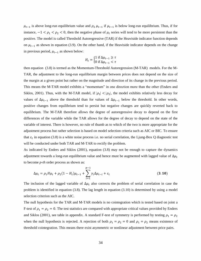
34

𝜇𝑡−1 is above long-run equilibrium value and 𝜌2 𝜇𝑡−1 if 𝜇𝑡−1 is below long-run equilibrium. Thus, if for

instance, −1 < 𝜌1 < 𝜌2 < 0, then the negative phase of 𝜇𝑡 series will tend to be more persistent than the

positive. The model is called Threshold Autoregressive (TAR) if the Heaviside indicator function depends

on 𝜇𝑡−1 as shown in equation (3.9). On the other hand, if the Heaviside indicator depends on the change

in previous period, 𝜇𝑡−1 as shown below:

𝐻𝑡 = {1 if ∆𝜇𝑡−1 ≥ 𝜏0 if ∆𝜇𝑡−1 < 𝜏

then equation (3.8) is termed as the Momentum-Threshold Autoregression (M-TAR) models. For the M-

TAR, the adjustment to the long-run equilibrium margin between prices does not depend on the size of

the margin at a given point but rather on the magnitude and direction of its change in the previous period.

This means the M-TAR model exhibits a “momentum” in one direction more than the other (Enders and

Siklos, 2001). Thus, with the M-TAR model, if 𝜌1 < 𝜌2, the model exhibits relatively less decay for

values of ∆𝜇𝑡−1 above the threshold than for values of ∆𝜇𝑡−1 below the threshold. In other words,

positive changes from equilibrium tend to persist but negative changes are quickly reverted back to

equilibrium. The M-TAR therefore allows the degree of autoregressive decay to depend on the first

differences of the variable while the TAR allows for the degree of decay to depend on the state of the

variable of interest. There is however, no rule of thumb as to which of the two is more appropriate for the

adjustment process but rather selection is based on model selection criteria such as AIC or BIC. To ensure

that 휀𝑡 in equation (3.8) is a white noise process i.e. no serial correlation, the Ljung-Box Q diagnostic test

will be conducted under both TAR and M-TAR to rectify the problem.

As indicated by Enders and Siklos (2001), equation (3.8) may not be enough to capture the dynamics

adjustment towards a long-run equilibrium value and hence must be augmented with lagged value of ∆𝜇𝑡

to become p-th order process as shown as:

∆𝜇𝑡 = 𝜌1𝐻𝜇𝑡 + 𝜌2(1 − 𝐻𝑡)𝜇𝑡−1 + ∑ 𝛾𝑖∆𝜇𝑡−𝑖

𝑝−1

𝑖=1

+ 휀𝑡 (𝟑. 𝟏𝟎)

The inclusion of the lagged variable of ∆𝜇𝑡 also corrects the problem of serial correlation in case the

problem is identified in equation (3.8). The lag length in equation (3.10) is determined by using a model

selection criterion such as the AIC.

The null hypothesis for the TAR and M-TAR models is no cointegration which is tested based on joint a

F-test of 𝜌1 = 𝜌2 = 0. The test statistics are compared with appropriate critical values provided by Enders

and Siklos (2001), see table in appendix. A standard F-test of symmetry is performed by testing 𝜌1 = 𝜌2

when the null hypothesis is rejected. A rejection of both 𝜌1 = 𝜌2 = 0 and 𝜌1 = 𝜌2 means existence of

threshold cointegration. This means there exist asymmetric or nonlinear adjustment between price pairs.

35

In general, the threshold value () is unknown in the estimation of TAR and M-TAR and hence needs to

be estimated with the values of 𝜌1 and 𝜌2. However, according to Enders and Siklos (2001), is

normally set to zero in most economic applications so that the cointegrating vector coincides with the

attractor. Following Otoo (2012), the threshold value in this study is initially set to zero in TAR and M-

TAR and afterwards estimated using the method proposed by Chan (1993).This methodology involves a

grid search over potential threshold values that minimize the sum of square residuals from the fitted TAR

or M-TAR. It is implemented by sorting all the lagged values of 𝜇𝑡in series from equation (3.5) and the

first difference of the lagged 𝜇𝑡 series in ascending order for both TAR and M-TAR respectively i.e.

𝜇1 < 𝜇2 < ⋯ < 𝜇𝑇 for TAR and ∆𝜇1 < ∆𝜇2 < ⋯ < ∆𝜇𝑇 for M-TAR where T represents the number of

observations used. The largest and smallest 15% of the values are discarded and each of the remaining

70% of the values is considered as a potential threshold value which is used to individually estimate

equation (3.10). The value that yields the lowest residual sum of square is chosen as the threshold value

and it is used to estimate either the consistent TAR or M-TAR model.

3.2.4 Modelling short-run dynamics of price linkages

Threshold Vector Error Correction Models

The above models deal with long-run price relationships and after they have been used to establish that

price series are linked or cointegrated, the vector error correction model (VECM) is used to analyze the

short-run dynamics (Enders and Granger, 1998). This study will therefore use the VECM to achieve the

objective of investigating the short-run dynamics between the reference market and the other regional

markets in Ghana. The VECM helps to estimate the speed at which a deviation of prices from equilibrium

is restored. The estimation of the error correction model depends on which of the symmetric or

asymmetric model is accepted from the cointegration analysis. Given that price adjustment is

asymmetric, then the asymmetric error correction model with local market price as dependent variables

can be specified as:

∆𝑃𝑡𝑙 = 𝛼° + ∑ 𝛼𝑗∆𝑃𝑡−𝑗

𝑙

𝑘

𝑗=1

+ ∑ 𝛾𝑗∆𝑃𝑡−𝑗𝑟

𝑚

𝑗=1

+ 1+𝐻𝑡𝜇𝑡−1 + 2

−(1 − 𝐻𝑡)𝜇𝑡−1 + 𝜖1𝑡 (𝟑. 𝟏𝟏)

∆𝑃𝑡𝑟 = 𝛼° + ∑ 𝛼𝑗∆𝑃𝑡−𝑗

𝑟

𝑘

𝑗=1

+ ∑ 𝛾𝑗∆𝑃𝑡−𝑗𝑙

𝑚

𝑗=1

+ 1+𝐻𝑡𝜇𝑡−1 + 2

−(1 − 𝐻𝑡)𝜇𝑡−1 + 𝜖1𝑡 (𝟑. 𝟏𝟐)

where 𝛼°, 𝛼𝑗, 𝛾𝑗 ,1+and 2

− are parameters to be estimated in the model, 𝐻𝑡 is the corresponding Heaviside

indicator from the threshold autoregressive model and 𝜖1𝑡 is the error term with zero mean and constant

36

variance. Theoretically, the TAR/M-TAR models indicate only cointegration relationships but not

causality. The vector error correction model is therefore useful in remedying this problem by determining

the direction of causality between selected regional yam markets. For that matter, equations (3.11) and

(3.12) will be estimated for all market pairs to ascertain the direction of causality between all regional

markets. The VECM basically implies any change in local market prices is the sum of both long-run

impact of the deviations from equilibrium value and the short-run effect of change in the central/reference

market on the local market price. 1+and 2

− are the long-run adjustment coefficients while 𝛾𝑗 is the short-

run adjustment coefficient. Using the Wald test, the Granger causality tests are performed by examining

whether the joint significance of all 𝛾𝑗 are statistically different from zero i.e. 𝛾0 = 𝛾1 = ⋯ = 0 (which

implies short-term causality) or whether all 𝛾𝑗 are significant (which implies long term causality). The

model will also reveal whether there is one-way causality or bi-directional causality from the different

market pairs.

Finally, the length of time needed for complete transmission of price shock or complete adjustment will

be analyzed from the VECM by impulse-responses calculations.

The general framework of the research methodology is summarized below.

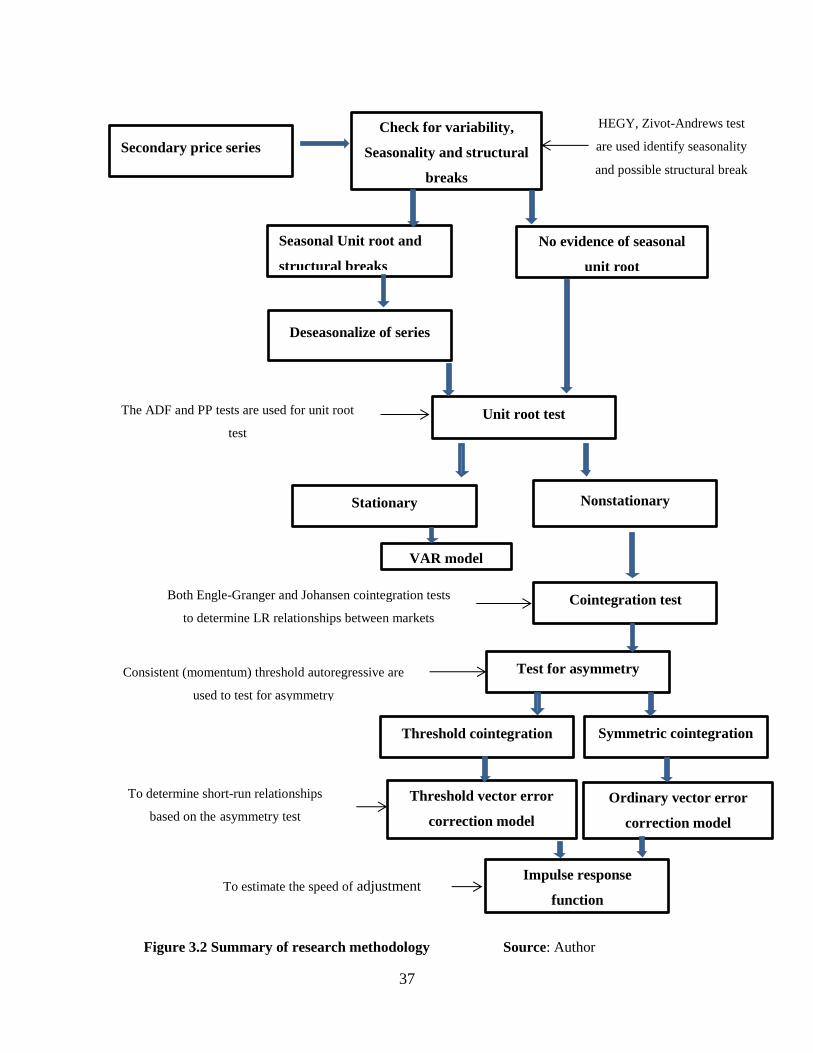
37

Figure 3.2 Summary of research methodology Source: Author

Secondary price series

Check for variability,

Seasonality and structural

breaks

Seasonal Unit root and

structural breaks

No evidence of seasonal

unit root

Deseasonalize of series

Unit root test

Stationary Nonstationary

Cointegration test

Test for asymmetry

Threshold cointegration Symmetric cointegration

Threshold vector error

correction model

Ordinary vector error

correction model

Impulse response

function

HEGY, Zivot-Andrews test

are used identify seasonality

and possible structural break

The ADF and PP tests are used for unit root

test

Both Engle-Granger and Johansen cointegration tests

to determine LR relationships between markets

Consistent (momentum) threshold autoregressive are

used to test for asymmetry

To determine short-run relationships

based on the asymmetry test

To estimate the speed of adjustment

VAR model

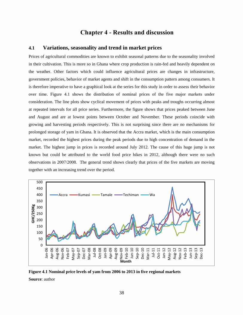
38

Chapter 4 - Results and discussion

4.1 Variations, seasonality and trend in market prices

Prices of agricultural commodities are known to exhibit seasonal patterns due to the seasonality involved

in their cultivation. This is more so in Ghana where crop production is rain-fed and heavily dependent on

the weather. Other factors which could influence agricultural prices are changes in infrastructure,

government policies, behavior of market agents and shift in the consumption pattern among consumers. It

is therefore imperative to have a graphical look at the series for this study in order to assess their behavior

over time. Figure 4.1 shows the distribution of nominal prices of the five major markets under

consideration. The line plots show cyclical movement of prices with peaks and troughs occurring almost

at repeated intervals for all price series. Furthermore, the figure shows that prices peaked between June

and August and are at lowest points between October and November. These periods coincide with

growing and harvesting periods respectively. This is not surprising since there are no mechanisms for

prolonged storage of yam in Ghana. It is observed that the Accra market, which is the main consumption

market, recorded the highest prices during the peak periods due to high concentration of demand in the

market. The highest jump in prices is recorded around July 2012. The cause of this huge jump is not

known but could be attributed to the world food price hikes in 2012, although there were no such

observations in 2007/2008. The general trend shows clearly that prices of the five markets are moving

together with an increasing trend over the period.

Figure 4.1 Nominal price levels of yam from 2006 to 2013 in five regional markets

Source: author

0

50

100

150

200

250

300

350

400

450

500

Jan

-06

Ap

r-0

6

Au

g-0

6

No

v-0

6

Feb

-07

May

-07

Sep

-07

De

c-0

7

Mar

-08

Jul-

08

Oct

-08

Jan

-09

Ap

r-0

9

Au

g-0

9

No

v-0

9

Feb

-10

Jun

-10

Sep

-10

De

c-1

0

Mar

-11

Jul-

11

Oct

-11

Jan

-12

May

-12

Au

g-1

2

No

v-1

2

Feb

-13

Jun

-13

Sep

-13

De

c-1

3

GH

C/2

50

Kg

Month

Accra Kumasi Tamale Techiman Wa

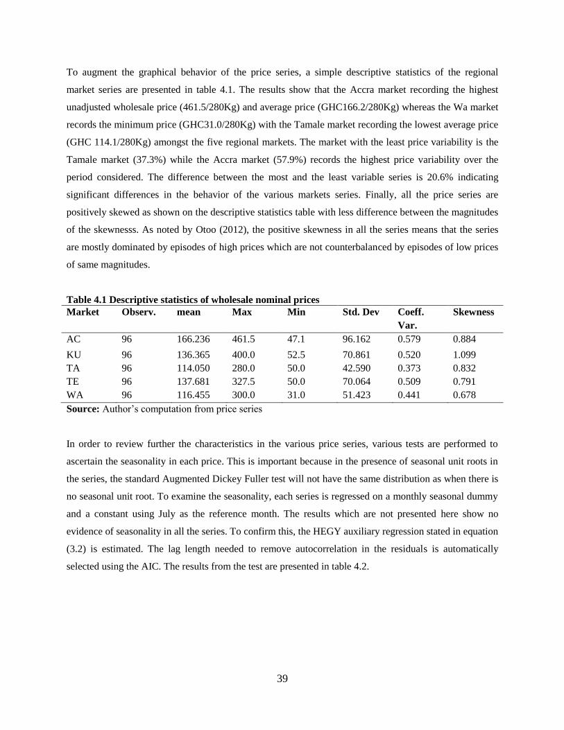
39

To augment the graphical behavior of the price series, a simple descriptive statistics of the regional

market series are presented in table 4.1. The results show that the Accra market recording the highest

unadjusted wholesale price (461.5/280Kg) and average price (GHC166.2/280Kg) whereas the Wa market

records the minimum price (GHC31.0/280Kg) with the Tamale market recording the lowest average price

(GHC 114.1/280Kg) amongst the five regional markets. The market with the least price variability is the

Tamale market (37.3%) while the Accra market (57.9%) records the highest price variability over the

period considered. The difference between the most and the least variable series is 20.6% indicating

significant differences in the behavior of the various markets series. Finally, all the price series are

positively skewed as shown on the descriptive statistics table with less difference between the magnitudes

of the skewnesss. As noted by Otoo (2012), the positive skewness in all the series means that the series

are mostly dominated by episodes of high prices which are not counterbalanced by episodes of low prices

of same magnitudes.

Table 4.1 Descriptive statistics of wholesale nominal prices

Market Observ. mean Max Min Std. Dev Coeff.

Var.

Skewness

AC 96 166.236 461.5 47.1 96.162 0.579 0.884

KU 96 136.365 400.0 52.5 70.861 0.520 1.099

TA 96 114.050 280.0 50.0 42.590 0.373 0.832

TE 96 137.681 327.5 50.0 70.064 0.509 0.791

WA 96 116.455 300.0 31.0 51.423 0.441 0.678

Source: Author’s computation from price series

In order to review further the characteristics in the various price series, various tests are performed to

ascertain the seasonality in each price. This is important because in the presence of seasonal unit roots in

the series, the standard Augmented Dickey Fuller test will not have the same distribution as when there is

no seasonal unit root. To examine the seasonality, each series is regressed on a monthly seasonal dummy

and a constant using July as the reference month. The results which are not presented here show no

evidence of seasonality in all the series. To confirm this, the HEGY auxiliary regression stated in equation

(3.2) is estimated. The lag length needed to remove autocorrelation in the residuals is automatically

selected using the AIC. The results from the test are presented in table 4.2.

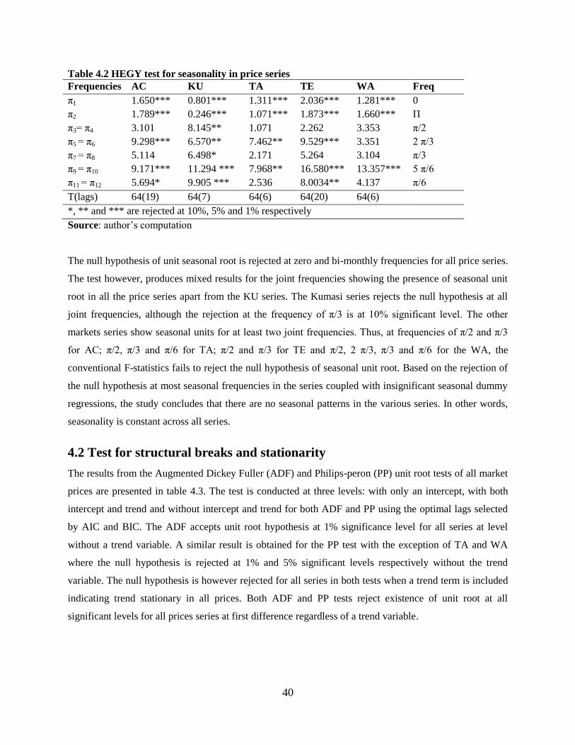
40

Table 4.2 HEGY test for seasonality in price series

Frequencies AC KU TA TE WA Freq

π1 1.650*** 0.801*** 1.311*** 2.036*** 1.281*** 0

π2 1.789*** 0.246*** 1.071*** 1.873*** 1.660*** Π

π3= π4 3.101 8.145** 1.071 2.262 3.353 π/2

π5 = π6 9.298*** 6.570** 7.462** 9.529*** 3.351 2 π/3

π7 = π8 5.114 6.498* 2.171 5.264 3.104 π/3

π9 = π10 9.171*** 11.294 *** 7.968** 16.580*** 13.357*** 5 π/6

π11 = π12 5.694* 9.905 *** 2.536 8.0034** 4.137 π/6

T(lags) 64(19) 64(7) 64(6) 64(20) 64(6)

*, ** and *** are rejected at 10%, 5% and 1% respectively

Source: author’s computation

The null hypothesis of unit seasonal root is rejected at zero and bi-monthly frequencies for all price series.

The test however, produces mixed results for the joint frequencies showing the presence of seasonal unit

root in all the price series apart from the KU series. The Kumasi series rejects the null hypothesis at all

joint frequencies, although the rejection at the frequency of π/3 is at 10% significant level. The other

markets series show seasonal units for at least two joint frequencies. Thus, at frequencies of π/2 and π/3

for AC; π/2, π/3 and π/6 for TA; π/2 and π/3 for TE and π/2, 2 π/3, π/3 and π/6 for the WA, the

conventional F-statistics fails to reject the null hypothesis of seasonal unit root. Based on the rejection of

the null hypothesis at most seasonal frequencies in the series coupled with insignificant seasonal dummy

regressions, the study concludes that there are no seasonal patterns in the various series. In other words,

seasonality is constant across all series.

4.2 Test for structural breaks and stationarity

The results from the Augmented Dickey Fuller (ADF) and Philips-peron (PP) unit root tests of all market

prices are presented in table 4.3. The test is conducted at three levels: with only an intercept, with both

intercept and trend and without intercept and trend for both ADF and PP using the optimal lags selected

by AIC and BIC. The ADF accepts unit root hypothesis at 1% significance level for all series at level

without a trend variable. A similar result is obtained for the PP test with the exception of TA and WA

where the null hypothesis is rejected at 1% and 5% significant levels respectively without the trend

variable. The null hypothesis is however rejected for all series in both tests when a trend term is included

indicating trend stationary in all prices. Both ADF and PP tests reject existence of unit root at all

significant levels for all prices series at first difference regardless of a trend variable.

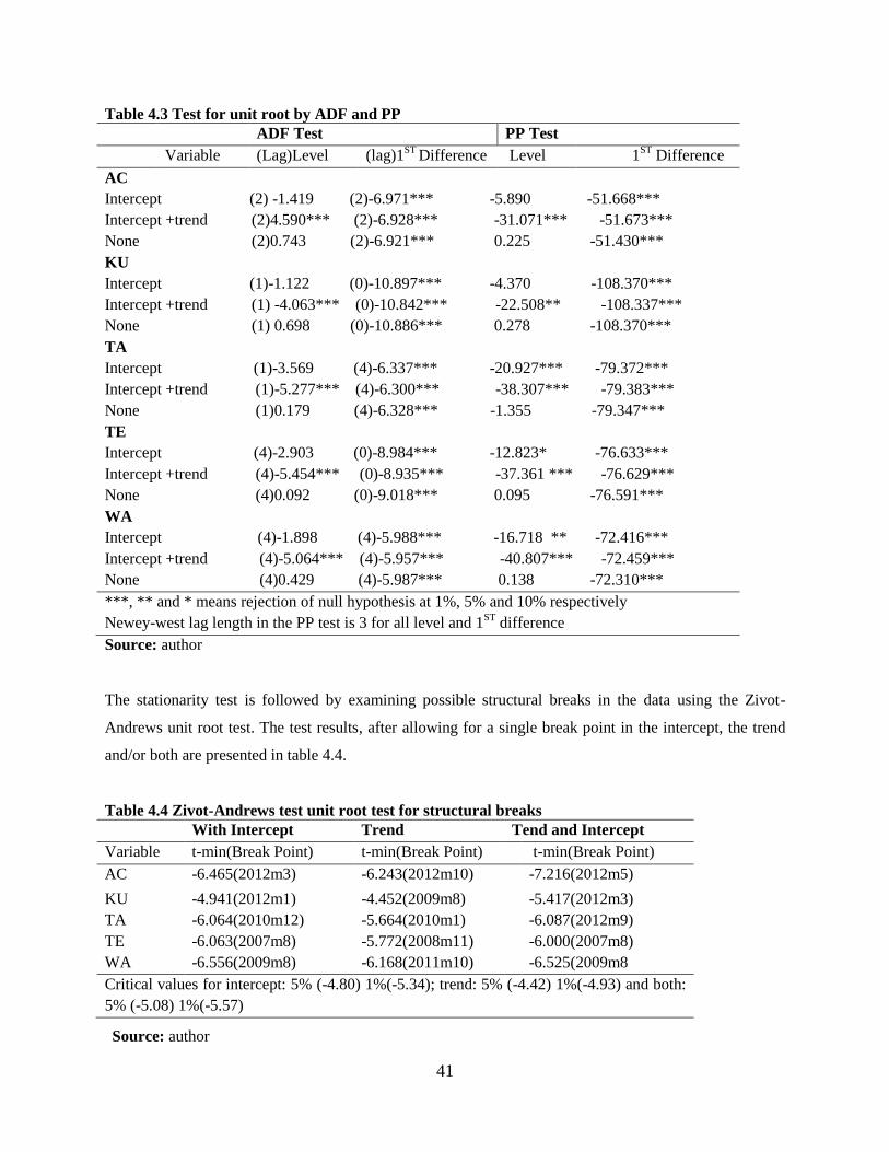
41

Table 4.3 Test for unit root by ADF and PP

ADF Test PP Test

Variable (Lag)Level (lag)1ST

Difference Level 1ST

Difference

AC

Intercept (2) -1.419 (2)-6.971*** -5.890 -51.668***

Intercept +trend (2)4.590*** (2)-6.928*** -31.071*** -51.673***

None (2)0.743 (2)-6.921*** 0.225 -51.430***

KU

Intercept (1)-1.122 (0)-10.897*** -4.370 -108.370***

Intercept +trend (1) -4.063*** (0)-10.842*** -22.508** -108.337***

None (1) 0.698 (0)-10.886*** 0.278 -108.370***

TA

Intercept (1)-3.569 (4)-6.337*** -20.927*** -79.372***

Intercept +trend (1)-5.277*** (4)-6.300*** -38.307*** -79.383***

None (1)0.179 (4)-6.328*** -1.355 -79.347***

TE

Intercept (4)-2.903 (0)-8.984*** -12.823* -76.633***

Intercept +trend (4)-5.454*** (0)-8.935*** -37.361 *** -76.629***

None (4)0.092 (0)-9.018*** 0.095 -76.591***

WA

Intercept (4)-1.898 (4)-5.988*** -16.718 ** -72.416***

Intercept +trend (4)-5.064*** (4)-5.957*** -40.807*** -72.459***

None (4)0.429 (4)-5.987*** 0.138 -72.310***

***, ** and * means rejection of null hypothesis at 1%, 5% and 10% respectively

Newey-west lag length in the PP test is 3 for all level and 1ST

difference

Source: author

The stationarity test is followed by examining possible structural breaks in the data using the Zivot-

Andrews unit root test. The test results, after allowing for a single break point in the intercept, the trend

and/or both are presented in table 4.4.

Table 4.4 Zivot-Andrews test unit root test for structural breaks

With Intercept Trend Tend and Intercept

Variable t-min(Break Point) t-min(Break Point) t-min(Break Point)

AC -6.465(2012m3) -6.243(2012m10) -7.216(2012m5)

KU -4.941(2012m1) -4.452(2009m8) -5.417(2012m3)

TA -6.064(2010m12) -5.664(2010m1) -6.087(2012m9)

TE -6.063(2007m8) -5.772(2008m11) -6.000(2007m8)

WA -6.556(2009m8) -6.168(2011m10) -6.525(2009m8

Critical values for intercept: 5% (-4.80) 1%(-5.34); trend: 5% (-4.42) 1%(-4.93) and both:

5% (-5.08) 1%(-5.57)

Source: author

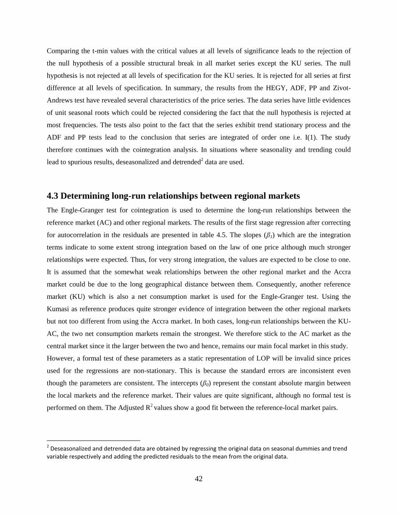
42

Comparing the t-min values with the critical values at all levels of significance leads to the rejection of

the null hypothesis of a possible structural break in all market series except the KU series. The null

hypothesis is not rejected at all levels of specification for the KU series. It is rejected for all series at first

difference at all levels of specification. In summary, the results from the HEGY, ADF, PP and Zivot-

Andrews test have revealed several characteristics of the price series. The data series have little evidences

of unit seasonal roots which could be rejected considering the fact that the null hypothesis is rejected at

most frequencies. The tests also point to the fact that the series exhibit trend stationary process and the

ADF and PP tests lead to the conclusion that series are integrated of order one i.e. I(1). The study

therefore continues with the cointegration analysis. In situations where seasonality and trending could

lead to spurious results, deseasonalized and detrended2 data are used.

4.3 Determining long-run relationships between regional markets

The Engle-Granger test for cointegration is used to determine the long-run relationships between the

reference market (AC) and other regional markets. The results of the first stage regression after correcting

for autocorrelation in the residuals are presented in table 4.5. The slopes (β1) which are the integration

terms indicate to some extent strong integration based on the law of one price although much stronger

relationships were expected. Thus, for very strong integration, the values are expected to be close to one.

It is assumed that the somewhat weak relationships between the other regional market and the Accra

market could be due to the long geographical distance between them. Consequently, another reference

market (KU) which is also a net consumption market is used for the Engle-Granger test. Using the

Kumasi as reference produces quite stronger evidence of integration between the other regional markets

but not too different from using the Accra market. In both cases, long-run relationships between the KU-

AC, the two net consumption markets remain the strongest. We therefore stick to the AC market as the

central market since it the larger between the two and hence, remains our main focal market in this study.

However, a formal test of these parameters as a static representation of LOP will be invalid since prices

used for the regressions are non-stationary. This is because the standard errors are inconsistent even

though the parameters are consistent. The intercepts (β0) represent the constant absolute margin between

the local markets and the reference market. Their values are quite significant, although no formal test is

performed on them. The Adjusted R2 values show a good fit between the reference-local market pairs.

2 Deseasonalized and detrended data are obtained by regressing the original data on seasonal dummies and trend

variable respectively and adding the predicted residuals to the mean from the original data.

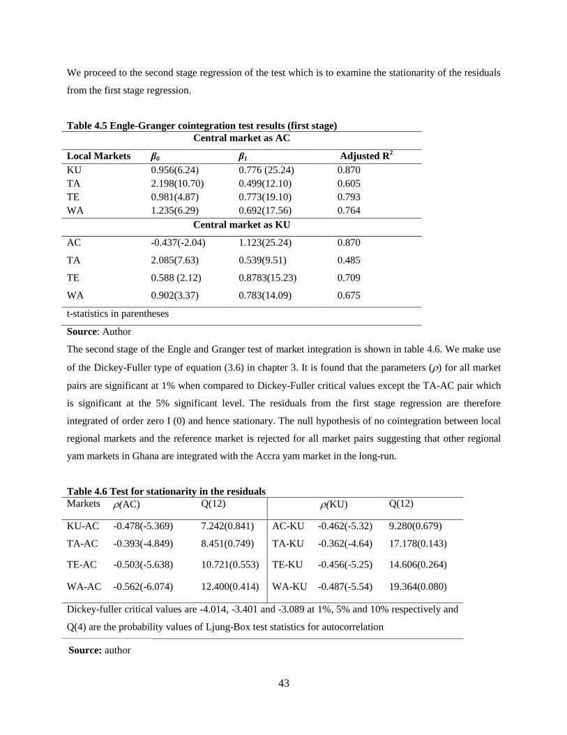
43

We proceed to the second stage regression of the test which is to examine the stationarity of the residuals

from the first stage regression.

Table 4.5 Engle-Granger cointegration test results (first stage)

Central market as AC

Local Markets β0 β1 Adjusted R2

KU 0.956(6.24) 0.776 (25.24) 0.870

TA 2.198(10.70) 0.499(12.10) 0.605

TE 0.981(4.87) 0.773(19.10) 0.793

WA 1.235(6.29) 0.692(17.56) 0.764

Central market as KU

AC -0.437(-2.04) 1.123(25.24) 0.870

TA 2.085(7.63) 0.539(9.51) 0.485

TE 0.588 (2.12) 0.8783(15.23) 0.709

WA 0.902(3.37) 0.783(14.09) 0.675

t-statistics in parentheses

Source: Author

The second stage of the Engle and Granger test of market integration is shown in table 4.6. We make use

of the Dickey-Fuller type of equation (3.6) in chapter 3. It is found that the parameters () for all market

pairs are significant at 1% when compared to Dickey-Fuller critical values except the TA-AC pair which

is significant at the 5% significant level. The residuals from the first stage regression are therefore

integrated of order zero I (0) and hence stationary. The null hypothesis of no cointegration between local

regional markets and the reference market is rejected for all market pairs suggesting that other regional

yam markets in Ghana are integrated with the Accra yam market in the long-run.

Table 4.6 Test for stationarity in the residuals

Markets (AC) Q(12) (KU) Q(12)

KU-AC -0.478(-5.369) 7.242(0.841) AC-KU -0.462(-5.32) 9.280(0.679)

TA-AC -0.393(-4.849) 8.451(0.749) TA-KU -0.362(-4.64) 17.178(0.143)

TE-AC -0.503(-5.638) 10.721(0.553) TE-KU -0.456(-5.25) 14.606(0.264)

WA-AC -0.562(-6.074) 12.400(0.414) WA-KU -0.487(-5.54) 19.364(0.080)

Dickey-fuller critical values are -4.014, -3.401 and -3.089 at 1%, 5% and 10% respectively and

Q(4) are the probability values of Ljung-Box test statistics for autocorrelation

Source: author

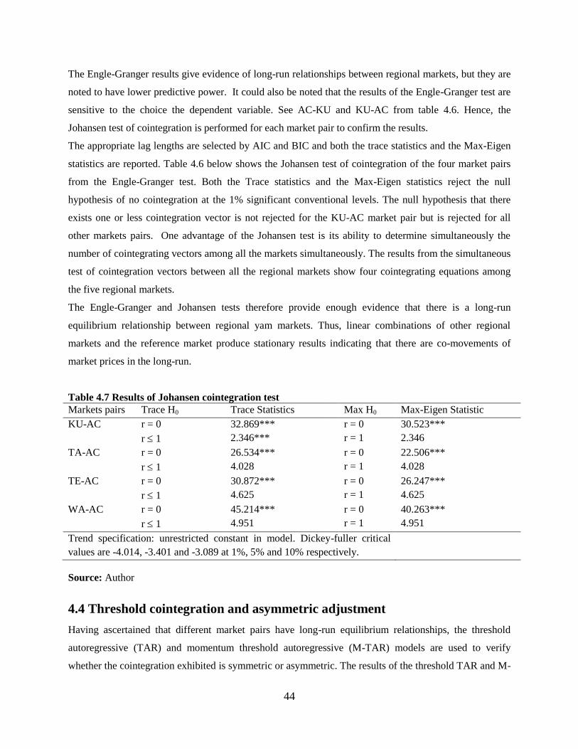
44

The Engle-Granger results give evidence of long-run relationships between regional markets, but they are

noted to have lower predictive power. It could also be noted that the results of the Engle-Granger test are

sensitive to the choice the dependent variable. See AC-KU and KU-AC from table 4.6. Hence, the

Johansen test of cointegration is performed for each market pair to confirm the results.

The appropriate lag lengths are selected by AIC and BIC and both the trace statistics and the Max-Eigen

statistics are reported. Table 4.6 below shows the Johansen test of cointegration of the four market pairs

from the Engle-Granger test. Both the Trace statistics and the Max-Eigen statistics reject the null

hypothesis of no cointegration at the 1% significant conventional levels. The null hypothesis that there

exists one or less cointegration vector is not rejected for the KU-AC market pair but is rejected for all

other markets pairs. One advantage of the Johansen test is its ability to determine simultaneously the

number of cointegrating vectors among all the markets simultaneously. The results from the simultaneous

test of cointegration vectors between all the regional markets show four cointegrating equations among

the five regional markets.

The Engle-Granger and Johansen tests therefore provide enough evidence that there is a long-run

equilibrium relationship between regional yam markets. Thus, linear combinations of other regional

markets and the reference market produce stationary results indicating that there are co-movements of

market prices in the long-run.

Table 4.7 Results of Johansen cointegration test

Markets pairs Trace H0 Trace Statistics Max H0 Max-Eigen Statistic

KU-AC r = 0

r 1

32.869***

2.346***

r = 0

r = 1

30.523***

2.346

TA-AC r = 0

r 1

26.534***

4.028

r = 0

r = 1

22.506***

4.028

TE-AC r = 0

r 1

30.872***

4.625

r = 0

r = 1

26.247***

4.625

WA-AC r = 0

r 1

45.214***

4.951

r = 0

r = 1

40.263***

4.951

Trend specification: unrestricted constant in model. Dickey-fuller critical

values are -4.014, -3.401 and -3.089 at 1%, 5% and 10% respectively.

Source: Author

4.4 Threshold cointegration and asymmetric adjustment

Having ascertained that different market pairs have long-run equilibrium relationships, the threshold

autoregressive (TAR) and momentum threshold autoregressive (M-TAR) models are used to verify

whether the cointegration exhibited is symmetric or asymmetric. The results of the threshold TAR and M-

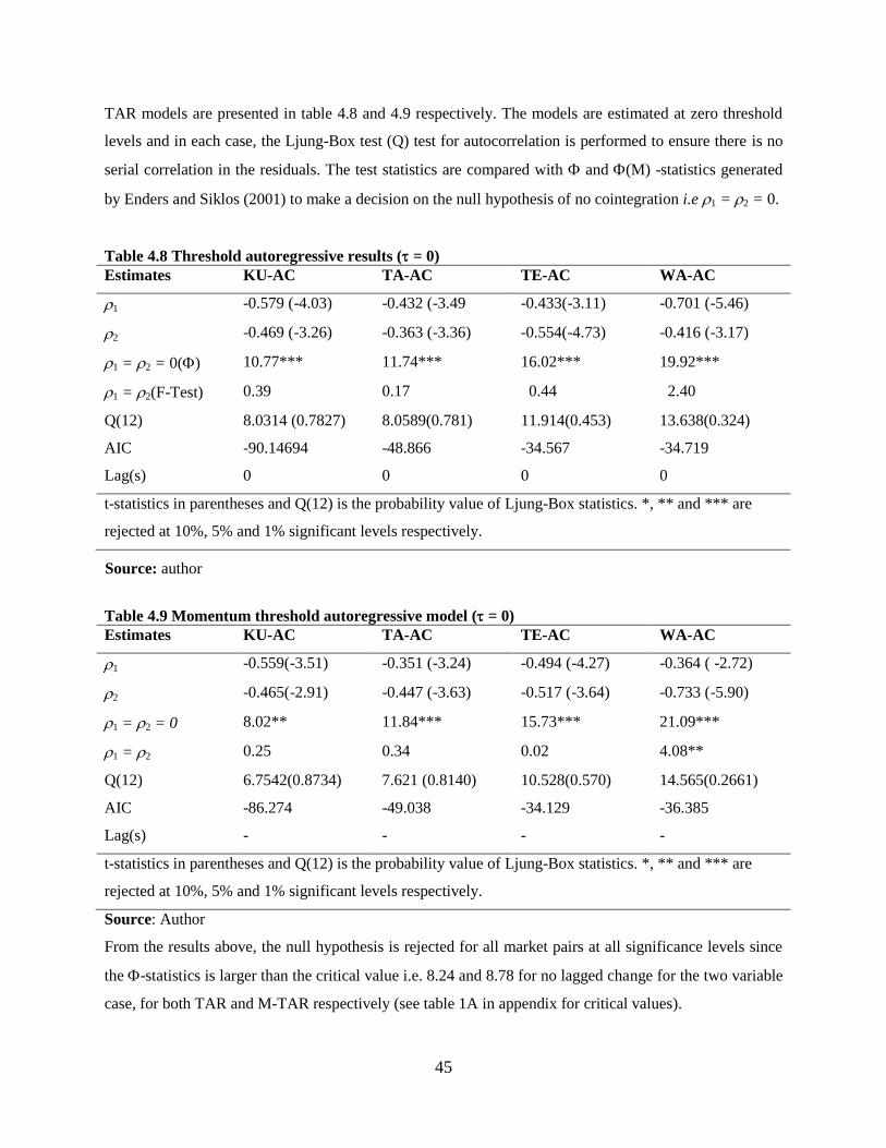
45

TAR models are presented in table 4.8 and 4.9 respectively. The models are estimated at zero threshold

levels and in each case, the Ljung-Box test (Q) test for autocorrelation is performed to ensure there is no

serial correlation in the residuals. The test statistics are compared with and (M) -statistics generated

by Enders and Siklos (2001) to make a decision on the null hypothesis of no cointegration i.e 1 = 2 = 0.

Table 4.8 Threshold autoregressive results ( = 0)

Estimates KU-AC TA-AC TE-AC WA-AC

1 -0.579 (-4.03) -0.432 (-3.49 -0.433(-3.11) -0.701 (-5.46)

2 -0.469 (-3.26) -0.363 (-3.36) -0.554(-4.73) -0.416 (-3.17)

1 = 2 = 0() 10.77*** 11.74*** 16.02*** 19.92***

1 = 2(F-Test) 0.39 0.17 0.44 2.40

Q(12) 8.0314 (0.7827) 8.0589(0.781) 11.914(0.453) 13.638(0.324)

AIC -90.14694 -48.866 -34.567 -34.719

Lag(s) 0 0 0 0

t-statistics in parentheses and Q(12) is the probability value of Ljung-Box statistics. *, ** and *** are

rejected at 10%, 5% and 1% significant levels respectively.

Table 4.9 Momentum threshold autoregressive model ( = 0)

Estimates KU-AC TA-AC TE-AC WA-AC

1 -0.559(-3.51) -0.351 (-3.24) -0.494 (-4.27) -0.364 ( -2.72)

2 -0.465(-2.91) -0.447 (-3.63) -0.517 (-3.64) -0.733 (-5.90)

1 = 2 = 0 8.02** 11.84*** 15.73*** 21.09***

1 = 2 0.25 0.34 0.02 4.08**

Q(12) 6.7542(0.8734) 7.621 (0.8140) 10.528(0.570) 14.565(0.2661)

AIC -86.274 -49.038 -34.129 -36.385

Lag(s) - - - -

t-statistics in parentheses and Q(12) is the probability value of Ljung-Box statistics. *, ** and *** are

rejected at 10%, 5% and 1% significant levels respectively.

Source: Author

From the results above, the null hypothesis is rejected for all market pairs at all significance levels since

the -statistics is larger than the critical value i.e. 8.24 and 8.78 for no lagged change for the two variable

case, for both TAR and M-TAR respectively (see table 1A in appendix for critical values).

Source: author

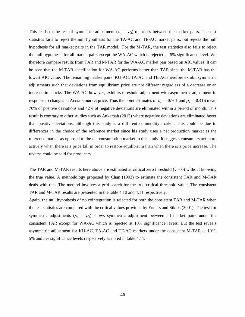
46

This leads to the test of symmetric adjustment (1 = 2) of prices between the market pairs. The test

statistics fails to reject the null hypothesis for the TA-AC and TE-AC market pairs, but rejects the null

hypothesis for all market pairs in the TAR model. For the M-TAR, the test statistics also fails to reject

the null hypothesis for all market pairs except the WA-AC which is rejected at 5% significance level. We

therefore compare results from TAR and M-TAR for the WA-AC market pair based on AIC values. It can

be seen that the M-TAR specification for WA-AC performs better than TAR since the M-TAR has the

lowest AIC value. The remaining market pairs: KU-AC, TA-AC and TE-AC therefore exhibit symmetric

adjustments such that deviations from equilibrium price are not different regardless of a decrease or an

increase in shocks. The WA-AC however, exhibits threshold adjustment with asymmetric adjustment in

response to changes in Accra’s market price. Thus the point estimates of 1 = -0.701 and 2 = -0.416 mean

70% of positive deviations and 42% of negative deviations are eliminated within a period of month. This

result is contrary to other studies such as Ankamah (2012) where negative deviations are eliminated faster

than positive deviations, although this study is a different commodity market. This could be due to

differences in the choice of the reference market since his study uses a net production market as the

reference market as opposed to the net consumption market in this study. It suggests consumers act more

actively when there is a price fall in order to restore equilibrium than when there is a price increase. The

reverse could be said for producers.

The TAR and M-TAR results here above are estimated at critical zero threshold ( = 0) without knowing

the true value. A methodology proposed by Chan (1993) to estimate the consistent TAR and M-TAR

deals with this. The method involves a grid search for the true critical threshold value. The consistent

TAR and M-TAR results are presented in the table 4.10 and 4.11 respectively.

Again, the null hypothesis of no cointegration is rejected for both the consistent TAR and M-TAR when

the test statistics are compared with the critical values provided by Enders and Siklos (2001). The test for

symmetric adjustments (1 = 2) shows symmetric adjustment between all market pairs under the

consistent TAR except for WA-AC which is rejected at 10% significance levels. But the test reveals

asymmetric adjustment for KU-AC, TA-AC and TE-AC markets under the consistent M-TAR at 10%,

5% and 5% significance levels respectively as noted in table 4.11.

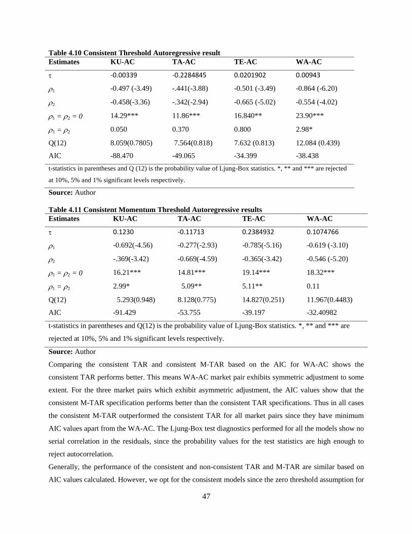
47

Table 4.10 Consistent Threshold Autoregressive result

Estimates KU-AC TA-AC TE-AC WA-AC

-0.00339 -0.2284845 0.0201902 0.00943

1 -0.497 (-3.49) -.441(-3.88) -0.501 (-3.49) -0.864 (-6.20)

2 -0.458(-3.36) -.342(-2.94) -0.665 (-5.02) -0.554 (-4.02)

1 = 2 = 0 14.29*** 11.86*** 16.840** 23.90***

1 = 2 0.050 0.370 0.800 2.98*

Q(12) 8.059(0.7805) 7.564(0.818) 7.632 (0.813) 12.084 (0.439)

AIC -88.470 -49.065 -34.399 -38.438

t-statistics in parentheses and Q (12) is the probability value of Ljung-Box statistics. *, ** and *** are rejected

at 10%, 5% and 1% significant levels respectively.

Source: Author

Table 4.11 Consistent Momentum Threshold Autoregressive results

Estimates KU-AC TA-AC TE-AC WA-AC

0.1230 -0.11713 0.2384932 0.1074766

1 -0.692(-4.56) -0.277(-2.93) -0.785(-5.16) -0.619 (-3.10)

2 -.369(-3.42) -0.669(-4.59) -0.365(-3.42) -0.546 (-5.20)

1 = 2 = 0 16.21*** 14.81*** 19.14*** 18.32***

1 = 2 2.99* 5.09** 5.11** 0.11

Q(12) 5.293(0.948) 8.128(0.775) 14.827(0.251) 11.967(0.4483)

AIC -91.429 -53.755 -39.197 -32.40982

t-statistics in parentheses and Q(12) is the probability value of Ljung-Box statistics. *, ** and *** are

rejected at 10%, 5% and 1% significant levels respectively.

Source: Author

Comparing the consistent TAR and consistent M-TAR based on the AIC for WA-AC shows the

consistent TAR performs better. This means WA-AC market pair exhibits symmetric adjustment to some

extent. For the three market pairs which exhibit asymmetric adjustment, the AIC values show that the

consistent M-TAR specification performs better than the consistent TAR specifications. Thus in all cases

the consistent M-TAR outperformed the consistent TAR for all market pairs since they have minimum

AIC values apart from the WA-AC. The Ljung-Box test diagnostics performed for all the models show no

serial correlation in the residuals, since the probability values for the test statistics are high enough to

reject autocorrelation.

Generally, the performance of the consistent and non-consistent TAR and M-TAR are similar based on

AIC values calculated. However, we opt for the consistent models since the zero threshold assumption for

48

the non-consistent TAR and M-TAR could be too strong. Based on this reason and model performance

revealed by AIC, the models selected for further analysis and inference are the consistent M-TAR for

KU-AC, TA-AC, TE-AC and consistent TAR for WA-AC.

The result from the consistent TAR for WA-AC in table 4.10 shows point estimates of 1 = -0.619 and 2

= -0.546. These values imply that approximately 62% of positive and 55% of negative price deviations

from equilibrium are eliminated within a period of one month. Thus, given that price series are at

equilibrium at period t but are moved out of this equilibrium by invisible market forces to new

equilibriums, then the results show that parts of the discrepancy from equilibrium will be eliminated in

the process. The rate at which the discrepancy is eliminated depends on whether the direction of shock is

positive or negative for asymmetry adjustment. For the WA-AC price pars, 62% of the discrepancy is

eliminated if the shock is positive and 55% if otherwise. This further implies that 38% of positive

discrepancy and 45% of negative discrepancy is carried over to the next month. Hence, the WA-AC

market responds quickly to shocks which increase profit margins between the two markets than shocks

which decrease the profit margin.

A similar trend is observed for the KU-AC and the TE-AC price pairs. In the KU-AC 69% of positive and

37% of negative deviations are eliminated within a period of one month meaning that 31% and 67% of

positive and negative discrepancies respectively persist for the following month. Again, this implies that

the market pair responds more quickly to shocks that stretch the profit margins than shocks that squeeze

the profit margins. For the TE-AC markets, approximately 79% of positive deviations and 37% of

negative discrepancies are eliminated after one month.

The TA-AC price pair however, responds differently to price shocks. From table 4.11, approximately

27% of positive deviations and 67% of negative deviations are eliminated within one month. This price

pair therefore responds more quickly to shocks which squeeze the profit margin than those which stretch

them. In other words, price falls are quickly adjusted compared to price increments between these two

markets. For prices between the different market pairs to adjust in the long-run when there is a

disequilibrium, it is expected that deviations exceed a certain threshold value due to the transaction costs

borne by market agents in the adjustment process. Using the threshold values generated as proxy for

transaction cost between market pairs as often hypothesized, we see that deviations must exceed certain

values before adjustments are triggered for the true models selected. Thus, for KU-AC and TA-AC,

absolute price deviations must exceed 12% before adjustment towards long-run equilibrium is triggered.

For the TE-AC and WA-AC, absolute price deviations must not be less than 23% and 0.9% respectively

in other to have an adjustment towards long-run equilibrium initiated.

49

4.5 Short-run relationships between regional markets

Having established that there are long-run relationships between other regional markets and the reference

market, the study seeks to analyze the short-run dynamics between the price series using the Vector Error

Correction Model (VECM). Table 4.12 below shows the asymmetric and symmetric VECM results from

equation (3.11) and (3.12).

The estimation of the VECM is based on results from the consistent threshold models. This means for

price pairs which exhibit consistent TAR cointegration, we estimate threshold VECM and vice versa.

Thus, the momentum threshold VECM is estimated for KU-AC, TA-AC AND TE-AC price pairs while

threshold VECM is estimated for WA-AC pair. For each model, we perform normality as well as the

Ljung-Box Q test on the residuals to ensure that residuals are white noise processes and follow a normal

distribution. The probability values at lag 12 of the Ljung-Box Q test are presented in tables of each

model. Also since the influence of the reference market is expected to be distributed over time, the AIC is

used to determine pre-estimation lag lengths for each model. The adjusted R2 of each model is reported to

show the extent to which variations in the dependent variables are explained by the right hand side

variables.

Adjustment of local markets to restore equilibrium are measured by the 𝑧_𝑝𝑙𝑢𝑠𝑡−1and 𝑧_𝑚𝑖𝑛𝑢𝑠𝑡−1 values

for each model. These values therefore indicate how quickly deviations in the long-run are corrected. It

can be seen from the first market pair, the KU-AC in table 4.12, that the adjustment coefficients are

significant for both positive and negative deviations at 10% and 1% levels respectively. The point

estimates show that the KU market adjust to eliminate 49% of a unit positive deviation within a month

while it adjusts to eliminate 34% of a unit negative deviation created by the AC market within the same

period. The AC market model also has both highly significant adjustments to positive and negative

deviations from equilibrium, although the speed of elimination of positive deviations is lower compared

to the KU model. For negative deviations, the AC models adjust quickly compared to the KU model.

There is therefore, asymmetry in terms of speed of adjustment for positive and negative deviation

between KU and AC. Thus, even though both markets respond to positive and negative price deviations

from equilibrium, the speed of response differs depending on whether deviations are positive or negative.

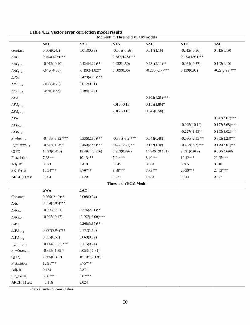
50

Table 4.12 Vector error correction model results Momentum Threshold VECM models

KU AC TA AC TE AC

constant 0.006(0.42) 0.013(0.93) -0.005(-0.26) 0.017(1.19) -0.012(-0.56) 0.013(1.19)

𝐴𝐶 0.493(4.79)*** 0.587(4.28)*** 0.473(4.93)***

𝐴𝐶𝑡−1 -0.012(-0.10) 0.424(4.22)*** 0.232(1.50) 0.231(2.11)** -0.064(-0.37) 0.102(1.10)

𝐴𝐶𝑡−2 -.042(-0.36) -0.190(-1.82)* 0.009(0.06) -0.268(-2.7)*** 0.139(0.95) -0.22(2.95)***

𝐾𝑈 0.429(4.79)***

𝐾𝑈𝑡−1 -.083(-0.70) 0.012(0.11)

𝐾𝑈𝑡−2 -.091(-0.87) 0.104(1.07)

𝑇𝐴 0.302(4.28)***

𝑇𝐴𝑡−1 -.015(-0.13) 0.155(1.86)*

𝑇𝐴𝑡−2 -.017(-0.16) 0.045(0.58)

𝑇𝐸 0.343(7.67)***

𝑇𝐸𝑡−1 -0.025((-0.19) 0.177(2.68)***

𝑇𝐸𝑡−2 -0.227(-1.93)* 0.185(3.02)***

𝑧_𝑝𝑙𝑢𝑠𝑡−1 -0.488(-3.92)*** 0.336(2.80)*** -0.381(-3.2)*** 0.043(0.48) -0.636(-2.15)** 0.353(2.23)**

𝑧_𝑚𝑖𝑛𝑢𝑠𝑡−1 -0.342(-1.96)* 0.450(2.83)*** -.444(-2.47)** 0.172(1.30) -0.493(-3.8)*** 0.149(2.01)**

Q(12) 12.33(0.410) 15.493 (0.216) 6.313(0.899) 17.805 (0.121) 3.631(0.989) 9.060(0.698)

F-statistics 7.28*** 10.13*** 7.91*** 8.40*** 12.42*** 22.25***

Adj. R2 0.323 0.410 0.345 0.360 0.465 0.618

SR_F-stat 10.54*** 8.70*** 9.38*** 7.73*** 20.39*** 26.53***

ARCH(1) test 2.003 3.520 0.771 1.438 0.244 0.077

Threshold VECM Model

WA AC

Constant 0.066( 2.10)** 0.008(0.34)

𝐴𝐶 0.554(3.85)***

𝐴𝐶𝑡−1 -0.099(-0.61) 0.276(2.51)**

𝐴𝐶𝑡−2 -0.025(-0.17) -0.292(-3.00)***

𝑊𝐴 0.268(3.85)***

𝑊𝐴𝑡−1 0.327(2.84)*** 0.132(1.60)

𝑊𝐴𝑡−2 0.055(0.51) 0.069(0.92)

𝑧_𝑝𝑙𝑢𝑠𝑡−1 -0.144(-2.07)*** 0.115(0.74)

𝑧_𝑚𝑖𝑛𝑢𝑠𝑡−1 -0.365(-1.89)* 0.0533( 0.39)

Q(12) 2.866(0.379) 16.108 (0.186)

F-statistics 12.91*** 8.75***

Adj. R2 0.475 0.371

SR_F-stat 5.80*** 8.82***

ARCH(1) test 0.116 2.024

Source: author’s computation

51

For TA-AC pairs, TA responds to both negative and positive deviations in the long-run price equilibrium

when there is a change in AC market prices. The AC does not respond to the changes in TA market

prices. The response of the TA prices to the AC is faster for negative deviation (44%) compared to a

positive deviation (38%) indicating negative asymmetry. In the final momentum threshold VECM, the

feedback mechanisms between prices of the TE-AC pair were symmetric in the sense that positive

discrepancies from equilibrium adjust faster than negative discrepancies regardless of which of the two

markets is used as the dependent variable.

The p-values of the SR_F-statistics for all the market in table 4.12 are significant at the 1% significant

level. This suggests contemporaneous and lagged changes of the independent variables (central market) in

each of the market pair significantly stimulate a response from the dependent variables (local markets) in

the short-run. This means we reject the null hypothesis that there are no short-run linkages between all

markets pairs. There is therefore two-way causality between all market pairs and hence an indication that

regional yam markets in Ghana are not segmented. The significant contemporaneous effects for all market

pairs mean that for instance, a 1% increase in AC market leads to 0.49%, 0.59% and 0.47% increases in

the KU, TA and TE markets respectively. This implies a decline in the marketing margin by 0.51%,

0.41% and 0.53% respectively. In the reverse situation, a 1% increase in the KU, TA and TE market

prices will increase prices in the AC market to 0.43%, 0.30% and 0.34% respectively.

From the threshold VECM, the results show that there is an asymmetry in terms of price feedbacks for the

WA-AC market pair. Thus, the point estimates suggest that the WA adjust to eliminate 14% and 37% of

positive and negative deviations caused by the AC market respectively, while the AC market neither

adjust to positive nor negative price deviations caused by WA markets. However, the joint hypothesis of

no short-run relationship is rejected at the 1% significance levels meaning there is a short-run linkage

between the two markets. This means the linkage is bi-directional as expected. Again, the

contemporaneous effect of a 1% increase in the price of the AC market leads to a 0.55% increase in the

WA market while a similar percentage increase of the WA market leads to a 0.27% increase in the AC

markets.

4.6 Impulse response estimation

From the various error correction models, we construct the impulse response functions. This gives

information about the magnitude of response to a price change in one market and the time needed to

restore equilibrium after a shock in the central market. For asymmetric adjustments, the response to a

price shock is dependent on the history of the time series as well as the sign (positive or negative) and

magnitude of the shock. Positive shocks are defined as shocks that lead to increment of the profit margin

52

for actors in the local markets i.e when there is a decrease in the reference or central market price while

negative shocks lead to a decrease in the profit margin of agents in the local markets (i.e increase in prices

of the reference market). The estimation of the impulse response function therefore helps to know the

time path required for a unit standard deviation shock in the central market to be eliminated from the

VECM models above.

As noted in table 4.12, our market pairs in the VECM are KU-AC, TA-AC, TE-AC and WA-AC. It can

be seen from the KU-AC pair that a 1 unit change in AC market price stimulates a 0.49 unit price change

in the KU market. If this change in the AC price is a 1% decrease/increase (i.e a positive/negative shock

to the profit margin of actors) then the KU market responds by increasing/decreasing by 0.49% (i.e

fall/rise in profit margins of actors). The decrease and increase in the profit margin by 0.51% (1-0.49) is

asymptotically corrected by a factor of 0.49 and 0.34 per period respectively in the following months as

the AC prices continue to increase or decrease. In the reverse situation, 1% change in KU market price

changes the AC market price by 0.43% leading to a 0.57%(1-0.43) shock to the profit margin. This is

corrected by a factor of 0.34 and 0.45 per period of one month for a decrease or increase respectively. The

results of the impulse response presented in figure A.1 and A.2 in appendix for KU-AC pair show that

price transmission from AC markets to KU market and vice versa. From the figure, it takes approximately

14 months for KU market margins to return to equilibrium after experiencing a negative shock (thus,

when there is an increase in AC market prices). However, it takes within 11months to return to

equilibrium when there is a positive shock (i.e when there is a decrease in AC market prices). For the AC

market response to changes in KU market prices, negative shocks are restored within 10 months while

positive shocks take approximately 13 months.

Following similar reasoning from the discussion above, the TA-AC impulse response function shows that

it takes approximately 16 months for the TA market price to adjust to negative shocks caused by AC

markets whereas it takes 9 months to adjust to positive shocks. The AC on the other hand, takes within 18

months to adjust to negative shocks in the TA market whereas positive shocks persist for a long time. For

the TE-AC market pair, the TE adjusts to restore equilibrium within 11 months for negative shocks

caused by AC while it takes within 8 months to adjust for a positive shock. The AC takes approximately

24 and 15 months to adjust for negative and positive shocks caused by changes in the TE market prices

respectively. Lastly, between the WA-AC market pair, the WA market adjusts within 11 months to

establish equilibrium in response to negative shocks caused by the AC prices while it takes 26 months to

adjust to positive shocks. In reverse, the AC takes 27 months to adjust to negative shocks caused by the

WA market whereas positive shocks persist for a very long time.

53

The rationale behind market integration studies using price transmission as mentioned in the introductory

chapter is to assess the efficiency of markets. This helps to avoid duplication of interventions (Goletti et

al. 1995). Thus, taking our five regional markets, the evidence of short-run and long-run relationships we

have established mean that a policy intervention in the reference market (AC) will eventually, be

experienced by all four other regional markets. For instance, any policy that leads to shortage in the AC

market is expected to lead to shortages in the KU, TA TE and WA markets. This is very important for a

developing country like Ghana where many depend on agriculture for livelihoods. A government policy

to raise price of yam producers could be initiated in the AC market. This also means that other

commodities which are complements or substitutes to yam could also be influenced through the yam

market. Nonetheless, the impact on of yam market integration on substitutes or complement commodities

is another broad area of price transmission studies which deals with inter-commodity. For instance,

cassava serves as substitute for some poor household in Ghana. This means, a study to assess the inter-

commodity price relationships between yam and cassava could be interesting to look at.

Our results point to the fact that there should be regional balance of yam since the markets are linked. As

stated in the chapter 1, yam production takes place in 7 out of the 10 regions in Ghana. Even though, we

studied only 5 regional markets, we expect the remaining markets to behave in a similar way. If that

happens to be the case, then a balance is expected between the yam-deficit and yam-surplus markets

(Delgado, 1980). This means households who depend on the crop may rely on the market system for

supply provided there is enough production from farmers.

However, the somewhat long periods of adjustment and the asymmetry of feedback between some

regional market pairs are worth pointing out. This implies the feedback received by producers and

consumers differ, when there is a shock to the market system equilibrium. The non-linear adjustment and

slow speed mean that there remain some impediments to full efficiency of yam markets in Ghana. Von

Cramon-Taubadel (1998) gave some reasons why we might observe such asymmetric relationships at

different market levels. Some of these factors include: delays in transportation from one region to another;

adjustment costs borne by market agents; market power, government interventions; price spreads between

the central and local markets and the mode of price data collection. Other factors include the

inventory/stock management behavior of market actors (Langyintuo, 2010), lack of bi-directional

information flow between markets (Abdulai 2000).

As noted by Ankamah (2012), for maize markets in Ghana, specific causes of asymmetries cannot be

pointed out directly. This is more so for this study, since we did not model explicitly, structural and

behavioral factors as found in Goletti et al. (1995). Nonetheless, a closer look at the yam marketing

dynamics in Ghana gives some indications of a few possible causes. Firstly, although the commodity is

54

not stored for long periods due to lack of storage facilities, transportation from one region takes a lot time

due to their bulky nature and the poor road connecting some of the local markets with the reference

market. The water transportation routes also take several days due to lack of Ferries and slow canoe

transportation. This could lead to delay in delivery and hence prevent swift adjustment of prices between

regional markets. We could also point out that the capacity of traders to determine the time of release of

products into markets to be a likely cause (Langyintuo, 2010). However, the perishable nature of yam,

which inhibits prolonged stocking, leaves this assertion open to verification. The issue of market power

and government intervention mentioned in some literature could be potential causes in the yam market.

Since we did not attempt to model market power in the process, we neither reject nor accept this as a

possible cause of asymmetry. On government interventions, although there have been several government

intervention in the root crop sector, such as the RTIMP, we do not have any evidence of market distortion

from such policies. However, information flow between markets can be ruled out since high penetration

of Information Communication Technology tools, such as mobile phones, have aided easy information

flow among regional markets. In any case, they could be the main reason why we find linkages between

regional markets both in the short-run and in long-run. Finally, on the mode of price recording, this could

be a very important factor considering the sensitivity of price transmission models to data frequency

(Amikuzuno, 2010). The data used for this study is a monthly data, which are recorded by averaging

weekly market prices. This may lead to loss of important information contained in the price series. Since

high frequency data are noted to capture the dynamics of price transmission better (Amikuzuno (2010),

we may also attribute the asymmetry to in the data recording process. A higher frequency data, such as

weekly, is needed to verify this claim.

55

Chapter 5 – Summary and conclusion

Intermittent fluctuations in world food prices raise food security concerns in many developing countries

including Ghana. Over the past decades, governments in Ghana and other donor partners have invested in

the root and tuber crop sector with the sole objective of boosting production in such crops where the

country is self-sufficient in terms of food balance sheets. However, the issue of distribution remains a

major problem without efficient marketing system. A well-integrated marketing system is needed to

distribute food from surplus regions to deficit regions. This will help improve welfare of both consumers

and producers of agricultural commodities and more so, considering the fact that the agricultural sector is

the second largest employer in Ghana. A good knowledge of price mechanisms also helps policy makers

to avoid duplication of interventions in markets that are linked. The author is also of the view that market

integration studies have focused mainly on the grain/cereal sector and much less on the root crop sector.

The objective of this study is therefore to determine the dynamics and price mechanism between the

regional yam markets in Ghana. By so doing, we adopted the cointegration approach to determine the

long-run relation and the vectors error correction model to determine the short-run relationships between

the central market (Accra) and local markets (Kumasi, Tamale, Techiman and Wa). We sought to also

determine whether there are linear or non-linear adjustments between the central market and other

regional markets as well as time period required for adjustments with the help of the consistent threshold

models and impulse response functions.

The study used secondary monthly wholesale price data from 2006 to 2013 to achieve its objectives.

Preliminary investigations of the price series show all the prices series are positively skewed meaning

there are possibly episodes of high price increases which are not counterbalanced by the same magnitude

of price falls. The coefficient of variations also showed quite significant differences between the various

price series. Stationarity assessment of the data revealed that they are all integrated of order one

processes. Thus, price series are non-stationary at levels without trend, but become stationary at first

difference. There was also no evidence of structural breaks in the data. The results for the main objectives

presented and discussed in chapter 4 show both short-run and long-run linkages between the central

market and other regional yam markets in Ghana. This shows that regional yam markets are integrated

and not isolated. These findings contradict Acquah et al. (2012) about cassava markets. We attribute this

to the fact that yam is more traded compared to cassava in Ghana. Yam is also exported and this could

drive linkages between the different regional markets.

56

However, we find adjustments between market pairs after a price shock to exhibit asymmetric feedbacks

with many markets responding faster to positive than negative shocks caused by the Accra market. Thus,

the Kumasi, Tamale and Techiman markets adjust faster to positive shocks (i.e deviations that increase

profit margin) whiles only the Wa markets adjust faster to negative shock (i.e deviation that decrease the

profit margin) caused by the Accra market. The adjustments of the Accra market in response to shocks

caused by other regional markets were mixed and in some cases the shocks persisted, indicating

unidirectional feedbacks.

We attribute the linkage between regional yam markets to improvement in communication tools, such as

mobile phones over the past decade. We point out a few possible causes of asymmetry. Improvement in

other infrastructures such as roads and efficient trucks for transporting the commodity could see much of

the asymmetries eliminated between regional yam markets in Ghana.

57

REFERENCES

Abdulai, A. (2000). Spatial price transmission and asymmetry in the Ghanaian maize market. Journal of

development economics, 63(2), 327-349.

Abdulai, A. (2007). Spatial and vertical price transmission in food staples market chains in Eastern and

Southern Africa: What is the evidence. In FAO Trade and Markets Division Workshop on Staple

Food Trade and Market Policy Options for Promoting Development in Eastern and Southern

Africa, Rome (pp. 1-2).

Acquah G. H., Micah A. J. and Owusu R. (2012): Price Transmission in Domestic Agricultural Markets:

Evidence from Selected Cassava Markets in Ghana, Journal of Sustainable Development in

Africa Vol. 14(5) pp 218-228.

Adom, P. K. (2014). Commodity-specific spatial integration: inter-commodity integration and

substitution between maize and sorghum in Ghana. Ghanaian Journal of Economics, 2, 49-76.

Aidoo, R. (2009). An analysis of yam consumption patterns in Ghanaian urban communities (Doctoral

Dissertation, School of Graduate Studies, Kwame Nkrumah University of Science &

Technology).

Alemu, Z. G., & Van Schalkwyk, H. D. (2008). Market integration in Mozambican maize markets.

African Books Collective.

Alderman, H. (1991). Prices and markets in Ghana. Washington, DC: Cornell Food and Nutrition Policy

Program.

Alderman, H. (1992). Intercommodity price transmittal. Analysis of Food Markets in Ghana. The World

Bank, WPS, 884.

Alderman, H., & Shively, G. (1996). Economic reform and food prices: Evidence from markets in Ghana.

World Development, 24(3), 521-534.

Amikuzuno, J. (2010). Spatial Price Transmission and Market Integration: In Agricultural Markets After

Liberalization in Ghana: Evidence from Fresh Tomato Markets. Suedwestdeutscher Verlag fuer

Hochschulschriften.

Amikuzuno, J. (2011). Border effects on spatial price transmission between fresh tomato markets in

Ghana and Burkina-Faso: Any case for promoting trans-border trade in West Africa?

Anaadumba P., (2013) Analysis of incentives and disincentives for yam in Ghana. Technical notes series,

MAFAP, FAO, Rome.

Ankamah-Yeboah, I. (2012). Spatial Price Transmission in the Regional Maize Markets in Ghana. MPRA

Paper.

Badiane, O., & Shively, G. E. (1998). Spatial integration, transport costs, and the response of local prices

to policy changes in Ghana. Journal of Development Economics, 56(2), 411-431.

Badiane, O., & Shively, G. E. (1997). The response of local maize prices to the 1983 currency

devaluation in Ghana (No. 12). International Food Policy Research Institute (IFPRI).

58

Bancroft, R. D. (2000). Relieving post-harvest constraints and identifying opportunities for improving the

marketing of fresh yam in Ghana, 1st January-31st March, 2000. Final Project Report No: R6505.

Natural Resources Institute, University of Greenwich, Chatham, Kent, UK, 51.

Barrett, C. B. (2005): Spatial Market Integration”. The New Palgrave Dictionary of Economics,

2nd Edition, London: Palgrave Macmillan. Edited by Lawrence E. Blume and Steven N. Durlauf

Barrett, C. B. (1996). Market analysis methods: are our enriched toolkits well suited to enlivened

markets?. American Journal of Agricultural Economics, 825-829.

Barrett, C. B., & Li, J. R. (2002). Distinguishing between equilibrium and integration in spatial price

analysis. American Journal of Agricultural Economics, 84(2), 292-307.

Baulch, B. (1997). Transfer costs, spatial arbitrage, and testing for food market integration. American

Journal of Agricultural Economics, 79(2), 477-487.

Baum, C. F. (2001). Stata: The language of choice for time series analysis. The Stata Journal, 1(1), 1-16.

Beaulieu, J. J., & Miron, J. A. (1993). Seasonal unit roots in aggregate US data. Journal of econometrics,

55(1), 305-328.

Brendstrup, B., Hylleberg, S., Nielsen, M. Ø., Skipper, L., & Stentoft, L. (2001). Seasonality in economic

models. University of Aarhus, Economics Working Paper, (2001-16).

Canova, F., & Hansen, B. E. (1995). Are seasonal patterns constant over time? A test for seasonal

stability. Journal of Business & Economic Statistics, 13(3), 237-252.

Chan, K. S. (1993). Consistency and limiting distribution of the least squares estimator of a threshold

autoregressive model. The annals of statistics, 520-533.

Chowa, S. E. T. (2014). Analysis of the effectiveness of modern information and communication

technologies on maize marketing efficiency in Malawi markets. IFPRI Working Paper 10,

November 2014.

Cirera, X., & Arndt, C. (2006). Measuring the Impact of Road Rehabilitation and the Liberalization

Trend on Spatial Market Efficiency in Maize Markets in Mozambique. mimeo.

Clemente, J., Montanes, A., & Reyes, M. (1998). Testing for a unit root in variables with a double change

in the mean. Economics Letters, 59(2), 175-182.

Deaton, A., & Laroque, G. (1992). On the behaviour of commodity prices. The Review of Economic

Studies, 59(1), 1-23.

Delgado, C. L. (1986). A variance components approach to food grain market integration in northern

Nigeria. American Journal of Agricultural Economics, 68(4), 970-979.

Egyir, I. S., Al-Hassan, R. M., & Abakah, J. K. (2011). The effect of ICT-based market information

services on the performance of agricultural markets: Experiences from Ghana. International

Journal of ICT Research and Development in Africa (IJICTRDA), 2(2), 1-13.

59

Enders, W., & Granger, C. W. J. (1998). Unit-root tests and asymmetric adjustment with an example

using the term structure of interest rates. Journal of Business & Economic Statistics, 16(3), 304-

311.

Enders, W., & Siklos, P. L. (2001). Cointegration and threshold adjustment. Journal of Business &

Economic Statistics, 19(2), 166-176.

Engle, R. F., & Granger, C. W. (1987). Co-integration and error correction: representation, estimation,

and testing. Econometrica: journal of the Econometric Society, 251-276.

Engle, R. F., & Yoo, B. S. (1987). Forecasting and testing in co-integrated systems. Journal of

econometrics, 35(1), 143-159.

FASDEPII (2008): Food and Agriculture Sector Development Policy Ghana, Ministry of Food and

Agriculture.

Fackler, P. L. (1996). Spatial Price Analaysis: A Methodological Review. Mimeo. Raleigh:

North Carolina State University

Fackler, P. L., & Goodwin, B. K. (2001). Spatial price analysis. Handbook of agricultural economics, 1,

971-1024.

Franses, P. H. (1991). Seasonality, non-stationarity and the forecasting of monthly time series.

International Journal of Forecasting, 7(2), 199-208.

Glynn, J., Perera, N., & Verma, R. (2007). Unit root tests and structural breaks: a survey with

applications. Faculty of Commerce-Papers, 455.

Godfray, H. C. J., Beddington, J. R., Crute, I. R., Haddad, L., Lawrence, D., Muir, J. F., & Toulmin, C.

(2010). Food security: the challenge of feeding 9 billion people. science, 327(5967), 812-818.

Goletti, F., Ahmed, R., & Farid, N. (1995). Structural determinants of market integration: The case of rice

markets in Bangladesh. The Developing Economies, 33(2), 196-198.

González-Rivera G. and Helfand S. M. (2001) Economic Development and the Determinants of Spatial

Integration in Agricultural Markets, Working Paper 01-28: Department of Economics, University

of California, Riverside, August.

Goodwin, B. K., Grennes, T. J., & McCurdy, C. (1999). Spatial price dynamics and integration in Russian

food markets. The Journal of Policy Reform, 3(2), 157-193.

Goodwin, B. K., & Schroeder, T. C. (1990). Testing Perfect spatial market integration: An Application to

regional US Cattle markets. North Central Journal of Agricultural Economics, 12(2), 173-186.

Granger, C. W. (1980). Testing for causality: a personal viewpoint. Journal of Economic Dynamics and

control, 2, 329-352.

60

Granger, C. W. (1988). Some recent development in a concept of causality. Journal of econometrics,

39(1), 199-211.

Granger, C. W., & Newbold, P. (1974). Spurious regressions in econometrics. Journal of econometrics,

2(2), 111-120.

GSS (2010). Ghana Statistical Service, National Population and Housing Census

GSS (2014). Ghana Statistical Service, Annual statistical report.

Harriss, B. (1983). There is method in my madness: Or is it vice versa?: Measuring agricultural market

performance. University of East Anglia.

Heien, D. M. (1980). Markup pricing in a dynamic model of the food industry. American Journal of

Agricultural Economics, 62(1), 10-18.

Hossain, M. I., & Verbeke, W. (2010). Evaluation of rice markets integration in Bangladesh. The

Lahore Journal of Economics 15: 2 (Winter 2010): pp. 77-96

Hylleberg, S., Engle, R. F., Granger, C. W., & Yoo, B. S. (1990). Seasonal integration and cointegration.

Journal of econometrics, 44(1), 215-238.

Jasdanwalla, Z. (1966). Marketing efficiency in Indian agriculture. Marketing efficiency in Indian

agriculture.

Johansen, S. (1988). Statistical analysis of cointegration vectors. Journal of economic dynamics and

control, 12(2), 231-254.

Johansen, S., & Juselius, K. (1990). Maximum likelihood estimation and inference on cointegration—

with applications to the demand for money. Oxford Bulletin of Economics and statistics, 52(2),

169-210.

Katengeza, S. P. (2009). Malawi Agricultural Commodity Exchange And Spatial Rice Market Integration

(No. 117804). Collaborative Masters Program in Agricultural and Applied Economics.

Langyintuo, A. S. (2010, September). Grain Distribution in Ghana under Imperfectly Competitive Market

Conditions. In AAAE Third Conference/AEASA 48th Conference, September (pp. 19-23).

Mengel, C., & Cramon-Taubadel, S. V. (2014). Distance and border effects on price transmission: A

meta-analysis (No. 37). Global Food Discussion Papers.

Mensah-Bonsu, A., Agyeiwaa-Afrane, A., & Kuwornu, J. K. (2011). Efficiency of the plantain marketing

system in Ghana: A co-integration analysis. Journal of Development and Agricultural Economics,

3(12), 593-601.

Meyer, J., & Cramon‐Taubadel, S. (2004). Asymmetric price transmission: a survey. Journal of

agricultural economics, 55(3), 581-611.

Mittal, A. (2009). The 2008 food price crisis: rethinking food security policies. UN.

61

Mohendru I. D. (1937). Some factors affecting the price of wheat in the Punjab. Publication No. 49

(Board of Economics Inquiries, Punjab Government)

Montañés, A., & Reyes, M. (1998). Effect of a shift in the trend function on Dickey–Fuller unit root tests.

Econometric Theory, 14(03), 355-363.

Muyatwa, V. P. (2000). The liberalization and integration of regional maize markets in Zambia (Doctoral

dissertation, University Microfilms International).

Negassa, A., & Myers, R. J. (2007). Estimating policy effects on spatial market efficiency: An extension

to the parity bounds model. American Journal of Agricultural Economics, 89(2), 338-352.

Negassa, A., Myers, R., & Gabre-Madhin, E. Z. (2003). Analyzing grain market efficiency in developing

countries (No. 63). International Food Policy Research Institute (IFPRI).

Nti, K., & Sackitey, C. (2010): Cassava becoming the mainstay of Ghana’s GDP. GNA report, 27th

July,

2010.

Obstfeld, M., & Taylor, A. M. (1997). Nonlinear aspects of goods-market arbitrage and adjustment:

Heckscher's commodity points revisited. Journal of the Japanese and international economies,

11(4), 441-479.

Otoo, E. A. (2012). Asymmetric Price Transmission between Local and Imported Rice Prices in Burkina

Faso. Journal of Economics & Behavioral Studies, 4(9).

Perron, P. (1989). The great crash, the oil price shock, and the unit root hypothesis. Econometrica:

Journal of the Econometric Society, 1361-1401.

Perron, P. (1997). Further evidence on breaking trend functions in macroeconomic variables. Journal of

econometrics, 80(2), 355-385.

Perron, P. (1990). Testing for a unit root in a time series with a changing mean. Journal of Business &

Economic Statistics, 8(2), 153-162.

Rahman, M. M., & Shahbaz, M. (2013). Do imports and foreign capital inflows lead economic growth?

Cointegration and causality analysis in Pakistan. South Asia Economic Journal, 14(1), 59-81.

Ravallion, M. (1986). Testing market integration. American Journal of Agricultural Economics, 68(1),

102-109.

Serebrennikov D., Gotz L., and Glauben T., (2014): Spatial integration of Russian domestic wheat

market. A paper presented at EAAE Congress, Agri-food and Rural Innovations for Healthier

Societies, Ljubljana, August 26-29, 2014

Sexton, R. J., Kling, C. L., & Carman, H. F. (1991). Market integration, efficiency of arbitrage, and

imperfect competition: methodology and application to US celery. American Journal of

Agricultural Economics, 73(3), 568-580.

62

Shively, G. E. (1996). Food price variability and economic reform: An ARCH approach for Ghana.

American Journal of Agricultural Economics, 78(1), 126-136.

Spiller, P. T., & Huang, C. J. (1986). On the extent of the market: wholesale gasoline in the northeastern

United States. The Journal of Industrial Economics, 131-145.

Spiller, P. T., & Wood, R. O. (1988). The estimation of transaction costs in arbitrage models. Journal of

Econometrics, 39(3), 309-326.

SRID-MoFA (2013): Statistical, Research and Information Directorate, Ministry of Food and Agriculture

Ghana, Fact and Figures, August.

Timmer, C. P. (1974). A model of rice marketing margins in Indonesia. Food Research Institute Studies,

(02).

Timmer, C. P. (1987). Corn marketing , chapter 8, in: C.P Timmer, ed. The corn economy of Indonesia.

Cornell University Press.

USAID (2005): United States Agency for International Development. West Africa Trade Hub: Export

Development Feasibility Study.

Vavra, P., & Goodwin, B. K. (2005). Analysis of price transmission along the food chain.

OECD Food,Agriculture and Fisheries Papers, No. 3, OECD Publishing.

von Cramon-Taubadel, S. (1998). Estimating asymmetric price transmission with the error correction

representation: An application to the German pork market. European review of agricultural

economics, 25(1), 1-18.

Zivot, E., & Andrews, D. W. K. (2002). Further evidence on the great crash, the oil-price shock, and the

unit-root hypothesis. Journal of Business & Economic Statistics, 20(1), 25-44.

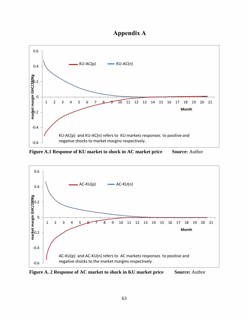
63

Appendix A

Figure A.1 Response of KU market to shock in AC market price Source: Author

Figure A. 2 Response of AC market to shock in KU market price Source: Author

-0.6

-0.4

-0.2

0

0.2

0.4

0.6

1 2 3 4 5 6 7 8 9 10 11 12 13 14 15 16 17 18 19 20 21

mar

ket

mar

gin

GH

C/2

80

Kg

Month

KU-AC(p) KU-AC(n)

KU-AC(p) and KU-AC(n) refers to KU markets responses to positive and negative shocks to market margins respectively .

-0.6

-0.4

-0.2

0

0.2

0.4

0.6

1 2 3 4 5 6 7 8 9 10 11 12 13 14 15 16 17 18 19 20 21

mar

ket

mar

gin

GH

C/2

80

Kg

Month

AC-KU(p) AC-KU(n)

AC-KU(p) and AC-KU(n) refers to AC markets responses to positive and negative shocks to the market margins respectively .

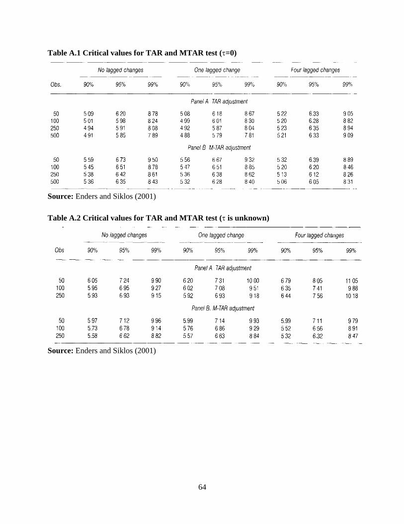
64

Table A.1 Critical values for TAR and MTAR test (=0)

Source: Enders and Siklos (2001)

Table A.2 Critical values for TAR and MTAR test ( is unknown)

Source: Enders and Siklos (2001)