integrating land survey data into measurement-based gis
TRANSCRIPT
INTEGRATING LAND SURVEY DATA
INTO MEASUREMENT-BASED GIS:
AN ASSESSMENT OF CHALLENGES AND PRACTICAL SOLUTIONS
FOR SURVEYORS IN TEXAS
by
Craig D. Bartosh
____________________________________________________________
A Thesis Presented to the
FACULTY OF THE USC GRADUATE SCHOOL
UNIVERSITY OF SOUTHERN CALIFORNIA
In Partial Fulfillment of the
Requirements for the Degree
MASTER OF SCIENCE
(GEOGRAPHIC INFORMATION SCIENCE AND TECHNOLOGY)
August 2012
Copyright 2012 Craig D. Bartosh

ii
Acknowledgments
I would like to take this opportunity to thank the many individuals who devoted
their time and efforts to complete this thesis research. Their continued guidance and
encouragement helped me persevere through the challenges of research. First, I would
like to thank my thesis faculty advisor Dr. Karen Kemp. Her infectious zeal and
eagerness to help find the right answer was a driving force in the completion of my
thesis. A special thanks to my other committee members Dr. Jordan Hastings and
Dr. Michael Goodchild. Dr. Hastings initially planted the seed that challenged me to
research measurement-based GIS. Dr. Goodchild, although not a University of Southern
California faculty member and was only a few months from retiring, chose to aid my
research and become a committee member. For the initial idea and willingness to be on
my committee, I will forever be grateful.
A very special thank you to individuals I was introduced to along the way. From
Esri, Brent Jones, Global Industry Manager – Survey/Cadastre/AEC. Thank you for the
hours of phone conversation and once again taking the time to explain the Parcel Editor.
Also from Esri, Tim Hodson, who also took the time and made an enormous effort to
help with my research. Finally, a special thanks to Byron Johnson, GCDB manager in
Nevada, for making the time for several phone conversations and providing publications
regarding the GCDB and its functionality.

iii
Table of Contents
Acknowledgments............................................................................................................... ii
List of Figures ..................................................................................................................... v
Abstract .............................................................................................................................. vi
Chapter 1: Introduction ....................................................................................................... 1
Chapter 2: Review of Literature ......................................................................................... 6
2.1 Land Surveying Background ..................................................................................... 7
2.2 GIS and Land Surveying ........................................................................................... 9
2.3 Measurement-Based GIS ......................................................................................... 13
2.4 MBGIS for Survey Data in Texas ........................................................................... 15
Chapter 3: Theoretical Model of MBGIS for Metes and Bounds Survey Data ................ 18
3.1 Functional Requirements of MBGIS for Survey Data ............................................ 18
3.2 Establishment of Control Points .............................................................................. 20
3.3 Upgradable Accuracy within a MBGIS .................................................................. 22
3.4 A Conceptual Model for Measurement Adjustment ............................................... 24
Chapter 4: Esri’s ArcGIS Parcel Fabric ............................................................................ 29
4.1 Measurement Elements of the Parcel Fabric ........................................................... 29
Table 1 Parcel Fabric Accuracy Table ..................................................................... 34
4.2 Examples of Measurement Elements ...................................................................... 36
4.2.1 Integrating Survey Data .................................................................................... 36
4.2.2 Establishing Control Points .............................................................................. 38
4.2.3 Adding Parcels.................................................................................................. 40
4.2.4 Failed Adjustment ............................................................................................ 43
4.2.5 Additional Test ................................................................................................. 45
Chapter 5: Towards the Management of Metes and Bounds Data in the Parcel Fabric ... 46
Chapter 6: Discussion ....................................................................................................... 52
Chapter 7: Conclusion....................................................................................................... 55
Glossary ............................................................................................................................ 58
References ......................................................................................................................... 61

iv
Appendix: Least-Squares Adjustment Results.................................................................. 64
Initial Least-squares Adjustment ................................................................................... 64
Least-Squares with three new Parcels ........................................................................... 66
Failed Results ................................................................................................................ 68

v
List of Figures
Figure 1: Geodetic Hierarchy 21
Figure 2: Interpolated Positions along a Surveyed Line Part 1 23
Figure 3: Interpolated Positions along a Surveyed Line Part 2 24
Figure 4: MBGIS Relationship Hierarchy for Survey Data 27
Figure 5: Connection Lines 31
Figure 6: Parcel Fabric Data Model 35
Figure 7: Initial CAD Import 37
Figure 8: Connection Lines within the Study Area 38
Figure 9: Parcel Coordinate Shifts 40
Figure 10: Adding Parcels 42
Figure 11: Failed Adjustment 43
Figure 12: Control Network Setup 48
Figure 13: Parent Tract Adjustment Regions 49

vi
Abstract
The land surveying community has discovered the economic benefits of managing
their survey data within a single system and view a geographic information system (GIS)
as a possible method of doing so. However, the traditional coordinate-based design of a
GIS does not contain the means to retain or employ the use of original measurements
collected by land surveyors, a legacy that has resulted in skepticism among the surveying
community. Thus, if a land surveyor desires to manage surveying data within a GIS
environment, that GIS should be a measurement-based GIS (MBGIS). This research
describes a MBGIS based upon the rules and relationships of measured points within the
metes and bounds surveying environment of the state of Texas. Since Esri’s parcel fabric
data model contains several characteristics that indicate it might be considered a
measurement-based system, it is explored as a possible method to manage and retain the
measurement-based elements of metes and bounds surveying within a GIS environment.
This study concludes that although the parcel fabric model has limitations when
compared to an ideal MBGIS, it does have the capability to manage metes and bounds
survey data if proper preparation and management techniques are applied.

1
Chapter 1: Introduction
The practice of land surveying involves working with measurements observed on
the ground to determine the boundary of a parcel of land (Robillard et al., 2003). In
contrast, a geographic information system (GIS) in its traditional practice defines a grid
coordinate system in which to locate objects for data analysis and visualization, often
compromising the integrity of ground measurements for the sake of creating a
homogenous product (Goodchild, 2002). There are many opportunities for surveyors to
integrate their work into traditional GIS practices, often improving upon the quality of the
GIS and further diversifying the role of a traditional land surveyor (Olaleye et al., 2011);
however, even with the recent contributions, the GIS community continues to fall victim
to skepticism from land surveyors because of its traditional coordinate-based approach
and early attention on data quantity as opposed to data quality (Deakin, 2008).
In contrast to Public Land Survey System (PLSS) regions, Texas is a metes and
bounds state, which does not require reference to a benchmark or the existence of a
geographic coordinate database (GCDB) when performing a land survey (Stamper,
1983). As a result, Texas surveyors typically create several arbitrary coordinate systems
at a local scale, which leads to a variety of coordinate datasets. As time progresses, some
coordinate datasets are consolidated, but as a whole, survey data remains divided,
creating the risk of duplicating field work and office research. As an employee of a land
surveying company in Texas, I have witnessed a lack of understanding of these problems
and the struggle to integrate numerous coordinate datasets into a central database to fully
derive the benefits of the data. Considerable time is wasted researching and pooling data

2
before a job can be completed. Most surveyors recognize that these problems could be
eliminated by having an integrated system (Jackson & Rambeau Sr., 2007). They also
recognize GIS as a popular solution, but have apprehension about the technology because
early GIS practices were not focused on survey-grade accuracy (Sorensen & Wetzel,
2007). As a result, GIS technology has been viewed as complementary to but not
sufficient for the profession (Deakin, 2008).
The initiative to integrate land survey data into GIS has been discussed heavily in
trade publications such as The American Surveyor and Professional Surveyor Magazine
and in many journal articles such as those noted above. Software vendors such as Esri,
the developer of the popular ArcGIS software, offer industry solutions to implement
survey data into GIS. Esri devotes a major section of their corporate website to the
management of land surveying and cadastral data.1 Often, however, the challenges of
data integration and the issues of data representation are rarely documented since the
usual solution is to purchase software and pay specialists to integrate data for surveyors..
Consequently, the end user fails to understand the technical aspects and issues involved
in the integration process. Lacking this knowledge has caused skepticism in the
surveying community, a profession built on knowledge of accuracy and error adjustments
in space (Jeffress, 2005).
The concept of a measurement-based geographic information system (MBGIS),
which stores and manipulates relative measures of distance and direction between points
rather than absolute coordinates for them, was formalized by Goodchild (2002). The key
1 Source: http://www.esri.com/industries/surveying/index.html

3
benefits of a MBGIS are its ability to calculate error and propagate adjustments
throughout the entire GIS database when a measurement changes. A traditional
coordinate-based GIS does not have this capability. It attempts to correct local areas
rather than adjusting the entire system, which may only make matters worse (Goodchild,
2002).
This research addresses the theoretical concept of managing metes and bounds
survey data within a MBGIS. If metes and bounds data is managed within a GIS, then it
must contain certain measurement-based characteristics for error analysis and have the
ability to retain original ground measurements to integrate with new measurements
obtained in the field. Section 2 of this document is a review of past literature that helps
support the argument that a MBGIS provides a suitable format to manage metes and
bounds survey data. Section 3 explores the design of a MBGIS that could be used to
manage and integrate metes and bounds survey data. As a supplement to these
background sections, a Glossary is included at the end of this document to insure that
technical surveying terms are used and understood consistently throughout this
document.
Although none of the concepts addressed in Section 3 are original, their inclusion
here still serves a purpose by addressing issues that arise when integrating survey data
into a MBGIS. Developing a MBGIS for a metes and bounds system offers unique
challenges because survey terminology and methodology are different than in PLSS
systems. Implementing the theory of MBGIS in the challenging survey environment of
Texas will indeed create new methodologies and may encourage the management of

4
survey coordinate datasets within a MBGIS. By incorporating measurement-based
adjustments and data representation methods traditionally used by surveyors into the
framework of a GIS data model, surveyors will become less apprehensive to use GIS as
their primary means of storing and manipulating survey data.
Section 4 of this document explores the parcel fabric data model within Esri’s
ArcGIS software. As research to complete this study progressed, the most recent design
of the parcel data model was discovered as a “best practice” attempt to incorporate and
retain original measurements from which parcels were derived. The parcel fabric, the
continuous surface of connected parcels defined by points and lines forming closed
polygons, within the data model incorporates ground distances when assessing error in
the overall coordinate model (Esri, 2011), which is a major characteristic of a MBGIS.
This data model also integrates highly accurate geodetic control points in the fabric
adjustment process, which is viewed as a successful method to integrate various
coordinate datasets into a single measurement-based system.
As reported later in Section 4, a small dataset of metes and bounds data, taken
from computer aided design (CAD) sources, was integrated into the parcel fabric to
display how common surveying data sources can be accommodated. Control points were
created in the fabric to illustrate the use of high-accuracy GPS technology within a
surveying environment. Additional metes and bounds data was then added to the fabric
and error adjustment processes were performed to explore the least-squares adjustment
process within the parcel fabric.

5
The results of these assessments were then used to formalize a methodology to
manage metes and bounds survey data within the parcel fabric. Section 5 illustrates
different methods to consider if one were to use the parcel fabric within a metes and
bounds surveying environment while maintaining the ultimate goal of administering
survey data within a GIS: integration of data into one system.
Section 6 of this document discusses the limitations of the parcel fabric in
relationship to the theory of a MBGIS. The coordinate-based design of the parcel fabric
is beneficial in terms of the visual representation of metes and bounds survey data.
Traditional GIS data visualization methods can greatly improve upon data representation
methods used in traditional surveying software. A MBGIS can potentially be used as a
dynamic tool to help determine boundaries as well as produce highly precise and accurate
maps for users, ultimately diversifying the business opportunities for survey companies.
However, there are still limitations to using the parcel fabric for metes and bounds survey
data. Although the current fabric dataset integrates ground measurements into the
system, the adjustment processes involving error are still performed within the coordinate
system. This does not allow for error propagation on the measured data itself, a
fundamental flaw of the data model when compared to the theory of MBGIS. As a final
point, future considerations of system design within the data model to better incorporate
the theory of MBGIS are mentioned.

6
Chapter 2: Review of Literature
Using measurements as the basic carriers of metric information is the key ingredient
in the design of a MBGIS (Buyong et al., 1991). If methods for incorporating ground-
measured data in a MBGIS can be easily understood, the surveying community may be
more willing to use the robust set of tools within a GIS environment. However, before a
theoretical model of a MBGIS for metes and bounds survey data can be formulated, there
are several topics that must be explored. The purpose of this review is to provide
background on the different themes that form the basis of this thesis research. The
review is divided into four sections as follows:
1. Land Surveying Background: A basic discussion of land surveying concepts is
provided, with primary focus on the semantics of metes and bounds surveying.
2. GIS and Land Surveying: Different methodologies of survey data integration into
GIS, including the creation of the abstract map from original survey field notes
for the General Land Office of Texas (GLO) and data integration into GIS from a
computer aided design (CAD) environment are discussed.
3. MBGIS: The theory of MBGIS, its brief history, and examples of the use and
evolution of MBGIS are explored.
4. MBGIS for Survey Data in Texas: The example of the geographic coordinate
database (GCDB) as a MBGIS is explained, and parallels from the three sections
above as well as the GCDB are drawn to form the basis of the conceptual model
used in this research.

7
2.1 Land Surveying Background
Land surveying is defined as the art of measuring and locating lines, angles, and
elevations of the surface of the earth, within underground workings, and on the beds of
bodies of water (U.S. Department of the Interior, 1973). Land in the modern state of
Texas was originally granted from the Mexican government and from the precursor
Republic of Texas in a different fashion than in PLSS states. Instead of being granted
sections and aliquot parts within a township & range cadastral system, Texans were
granted large acreages called “leagues” consisting of 4,428 acres. A married man was
granted an entire league, while a single man was given one-third of a league (Stamper,
1983). These grants, called abstracts, were given the name of the individual to whom the
land was granted. Today, the abstract remains the basis on which land is sold and
subdivided as metes and bounds tracts, defined as “…a description of real property that is
not described by reference to a lot or block shown on a map but is defined by starting at a
known point and describing, in sequence, the lines forming the boundaries of the
property” (Robillard et al., 2003).
Because of the growth of technology in surveying, metes and bounds tracts have
evolved into very precise and accurate depictions of ownership (Robillard et al., 2006).
They began as describing tracts of land in relation to who owned adjoining properties
(Stamper, 1983), but now consist of angles, distances, coordinate system references, and
detailed monumentation of corners (Robillard et al., 2003). It is the evolution and legal
statutes of metes and bounds surveys that form a semantic “rule guide” when surveyors
determine boundaries. The role of a surveyor in Texas is to collect and measure evidence
8
described in previous metes and bounds descriptions from the property boundary they are
determining as well as from adjoining properties, and establish the description of the
property being surveyed.
In Robillard et al. (2003, 2006), the authors discuss various scenarios of metes
and bounds legal descriptions and the procedures surveyors must follow to define a
boundary. Usually, each line segment in a metes and bounds description mentions an
angular direction, a distance, one or more monuments representing the line segment in
the field, and the adjoining property description. These items have different weights in
the decision of the surveyor in determining a property boundary. It is up to the surveyor
to determine the best evidence, but the order of importance is usually: monuments found
and measured in the field, adjoining legal descriptions, and finally bearing and distance.
When performing a boundary survey, surveyors usually begin with a sketch of the
property and adjoining properties they are surveying. This provides them with the
distances and monument calls within the area so a field crew knows what to look for at
each perceived property corner (Robillard et al., 2006). Once evidence is collected, the
data is usually downloaded to a computer for boundary calculations. The surveyor
checks measured angles and distances between found monumentation and interprets past
legal descriptions in the area to determine the boundary and write a legal description of
the property being surveyed. Collected data is commonly downloaded and manipulated
in a CAD environment, where a robust set of coordinate geometry tools are used to check
and calculate property corners (Olaleye et al., 2011).

9
No matter the amount of precision involved in the data collection process, errors
in surveying still occur (Robillard et al., 2006). These errors fall under three categories:
gross errors – blunders as a result of human error; systematic errors – errors within the
system or technology being used; and random errors – all unaccounted for errors. The
most famous method of error determination and adjustment calculation in surveying is
the least-squares adjustment method (Mikhail & Gracie, 1981). Least-squares is a
method of estimating values from a set of observations by minimizing the sum of the
squared differences between redundant observations. This method is incorporated into
most software packages used for surveying, including CAD software and GIS software
like Esri’s ArcGIS. The outcome of a least-squares adjustment in a computer
environment usually involves the output of error residuals and can be visualized by error
ellipses. These error residuals are associated with both measured points as well as
interpolated boundary corners.
2.2 GIS and Land Surveying
The benefits of integrating survey data into a GIS is a well-documented topic that
several different survey publications discuss on a monthly basis (see for example, Point
of Beginning and American Surveyor Magazine). Most focus on the business benefits of
having data in one database, and the advantages of base maps that offer vast amounts of
property and land visualization information in one file (Jackson & Rambeau Sr., 2007).
The ability of surveyors to overlay different GIS layers for visualization and management
purposes does indeed give users an advantage (Zimmer & Kirkpatrick, 2009). There is
no question that having files scanned, stored and linked to a GIS provides numerous

10
advantages over traditional file storage cabinets and paper copies (Corbley, 2001). These
initial practices of data management in GIS must be noted because their reliability and
use would only be increased within a MBGIS. This section discusses a few examples of
how survey data has been integrated into GIS as well as the skepticism that was created
between the two disciplines.
Data is integrated into a GIS several different ways, usually based on explicit
coordinates (Goodchild, 2002). This has traditionally been known as coordinate-based
GIS, resulting in processed and interpolated data where the integrity of the measurements
themselves is not retained (Goodchild, 2002). This coordinate-based methodology was
used by the General Land Office of Texas (GLO) to create the abstract layer base map for
the entire state. Abstract ownership maps created by the Tobin Map Company, which
originally created the maps for oil and mineral leasing purposes (P2 Energy Solutions,
2011), were digitized and georeferenced to form the base abstract map in Texas (General
Land Office of Texas, 2011). The inclusion of surveyor’s field notes has made the
original base map much more accurate, but its coordinate-based design remains the
driving force behind the GIS. Some data within the GLO’s base map is precise while
some is not. The ability to determine the amount of error in the different regions of the
abstract layer is not possible in the coordinate-based design (Goodchild, 2002). The
GLO’s base map stores and manages an enormous amount of survey data including links
to original copies of abstract legal descriptions, different mineral leases, their surveys,
and various other information such as submerged lands along the coast of Texas.
11
Since it is generally accepted that most surveyors have used a CAD environment
to calculate and store collected data measured in the field, the integration of survey data
from CAD into a GIS has become a common occurrence (Zimmer & Kirkpatrick, 2009).
Esri’s ArcGIS product has an entire toolset built to integrate CAD data. Sipes (2006)
highlights the historical differences between CAD and GIS. He states that CAD has
traditionally been used in architecture and engineering fields as a design tool, where GIS
has been used as a cartography and spatial analysis tool. Another difference he mentions
is that CAD is generally used on a project-by-project basis, while GIS is geared toward a
longer period of time; although, there have been recent software releases that use CAD
and GIS integration to build upon projects in the CAD environment (Carlson, 2011).
Sharing data between the two environments is usually done as an import where
CAD data is georeferenced or projected into GIS (Zimmer, 2011). Zimmer and
Kirkpatrick (2009) discuss integrating data using the Bureau of Land Management’s
(BLM) geographic coordinate data base (GCDB) as a control. This method involves the
use of GCDB measured data to adjust GIS data, a technique that is improving the
accuracy of GIS data in those states that use PLSS. However, no matter the methodology
to integrate survey data into GIS, the fundamental design of a coordinate-based GIS is
still intact, thus, from the surveyor’s perspective, ultimately degrading the integrity of the
data (Goodchild, 2002).
Advanced technology in the surveying fields has helped bridge the gap between
the two disciplines (Greenfeld, 2008) and recent articles suggest a movement towards
increasing the education of surveyors about the field of GIS. Felus (2007) discusses

12
several different concepts of GIS that are essential for surveying education including how
to integrate data into GIS for spatial analysis and data visualization purposes.
As technology and data integration has increased, the value of more accurate GIS
databases has been noted (Jeffress, 2003). As stated before, skepticism in the surveying
community arises from early GIS practices, which had a primary focus on getting data
into a system with less attention on accuracy of the data (Sorensen & Wetzel, 2007).
Deakin (2008) mentioned this as the reason why surveyors have always viewed GIS
technology as only being “complementary” to their profession, and few had greeted its
emergence with enthusiasm (Deakin, 2008).
However both Deakin (2008) and Sorensen and Wetzel (2007) state recent
movement in upgrading accuracy of spatial databases has sparked interest in surveying
professionals. Jeffress (2005) argues that the field of GIS needs surveyors because of
their understanding and knowledge of accuracy and error budgets. Zimmer and
Kirkpatrick (2009) also mention this in their article about improving GIS data accuracy
using survey data, noting that certain methods for integrating data can result in more
accurate and reliable GIS data (Zimmer & Kirkpatrick, 2009). Survey data has the
potential to play a large role in making GIS databases more accurate and more reliable,
but since it has been the tradition to integrate survey data into existing coordinate-based
GIS databases (Goodchild, 2002), the integrity of the survey data too often becomes
compromised.

13
2.3 Measurement-Based GIS
An early definition of a measurement-based GIS system comes from Buyong et
al. (1991). Such a system uses measurements as the basic carrier of metric information.
The authors defined the system as part of their conceptual model of a measurement-based
multipurpose cadastral system. They mention flaws in the cadastral system similar to that
mentioned in the section above, where measured data is integrated into coordinate data
and integrity is often compromised. They further argue that even though data within a
parcel cadastre is derived from surveyed legal descriptions, the implementation of the
coordinate-based system is substantially different from the traditional method of
surveying, where the relative positions between measured data is held in high regard.
The primary advantage offered by a measurement-based system is the ease of
updating - where the existence and value of each measurement are independent of each
other, and new measurements play a role in updating older measurements through least-
squares methods. The authors also cite incremental implementation as an advantage to a
measurement-based system—which is quite the opposite of many coordinate-based
systems—providing economic benefits for the implementation of a MBGIS. The most
important benefit is the continual improvement of accuracy based on measured data
points.
Following Buyong et al. (1991), Goodchild (2002) coined the term Measurement-
Based GIS (MBGIS), and distinguished it from the traditional coordinate-based GIS. He
argues that when data is stored in a coordinate-based system, its position becomes
absolute and fixed in space with no ability to correct or update the data without creating
14
geometric or topological distortions. Therefore any error between the rigid objects could
not fully be known. Contrary to the surveying community, Goodchild argues it is
traditional practice within the GIS community to assume the user can know the exact
location of objects in space.
Heo (2004) discusses the use of measurement-based data when building a
successful temporal land information system (LIS). Since surveyors are the primary
users of the system, basing the system on ground measurements is a necessity (Heo,
2004). He mentions four functional requirements to successfully incorporate measured
data into an LIS: measurement data retrieval, automatic coordinate update, spatial data
consistency checking, and blunder detection. These parts are similar to the architecture
proposed by Buyong et al. (1991). Within a measurement-based system, the three types
of errors—gross, systematic, and random (Mikhail & Gracie, 1981)—can be detected and
visualized in relation to other measured data (Heo, 2004). The ultimate decision process
of a surveyor involves the calculation of relative error between measured points on the
ground (Robillard et al., 2003). A system that can visualize these points based on
weighted controls and rules of methodology (Goodchild, 2002) are beneficial to the
surveying practice.
Building a GIS based on measured data and retaining the functions and
methodology of how the data was measured or derived, allows the possibility of
incremental correction and provides the user with estimates of the impact of measured
error, even when integrating data with different positional accuracy (Goodchild, 2002).
Measured points are not necessarily stored as static coordinates in space; rather, their

15
position is contingent upon their relationship with other measured points. After
establishing a set of rules to determine interpolated positions between measured points,
the means exist to detect and correct data that may be distorted due to errors in
measurement (Goodchild, 2002). This is not possible in a coordinate-based GIS.
2.4 MBGIS for Survey Data in Texas
The section above mentioned the benefits of a system that can visualize error
between measured points. Although this type of system has been achieved within a CAD
environment for the surveyor, it usually occurs at a very local scale. Therefore
measurements taken within a few blocks are retained in one file together, but have no
bearing upon the next block over, because its measurements are stored in a different file.
Some years ago Esri created an extension known as Survey Analyst that allowed for the
integration and display of measured data in a GIS. Navratil et al. (2004), tested the
capabilities of the Survey Analyst extension on cadastral data. The authors note the
ability of this MBGIS to improve the accuracy of the system as more accurate
measurements are placed within the system. They were able to adjust small parts of the
system just as the concept of MBGIS suggests. Although there were parts of the software
they did not like, they found the Survey Analyst extension to be a big step towards the
implementation of MBGIS. The Survey Analyst extension is no longer in existence and
has been replaced by the parcel fabric dataset and the Parcel Editor toolbar in ArcGIS
version 10.
The geographic coordinate database (GCDB) is the BLM’s initiative to create a
common coordinate database to reference within all federally owned lands (Wurm &

16
Hintz, 2003). The GCDB has also evolved into the closest example of a MBGIS for
survey data that is available to the public. All surveyed data within public lands in the
Western U.S. must use the GCDB as its coordinate reference (Zimmer & Kirkpatrick,
2009). With the development of the WINGMM (Windows-based Geographic
Measurement Management) software package which is a part of the National Integrated
Land System (NILS), the BLM has been able to integrate measured data into their
coordinate database (Zimmer & Kirkpatrick, 2009). The measured data is used to
estimate error on township and section corners from older surveys when technology and
accuracy were far inferior.
New technology in the surveying field has given the BLM a chance to weight the
different eras and methods of surveying into their system to better estimate and
understand error within their GIS. Wurm (2007) tested the GCDB’s ability to be updated
with more accurately measured data in a study undertaken at New Mexico State
University. He noted that the dynamic nature of the GCDB and its long-term
maintenance in which new measurements are added will improve the spatial accuracy
between points. As a MBGIS, the GCDB contains data whose location is established by
its measured position relative to other points in the system; has an upgradable accuracy
through some known function; and contains a set of rules to weight error within the
different eras and methods of survey data collection.
A MBGIS in a metes and bounds environment can be an ideal method of storing
and manipulating land survey data. Metes and bounds surveying contains a different set
of semantics than that of the PLSS, but can still fit within a MBGIS framework because

17
the weight of determination of a metes and bounds survey falls much greater upon found
and measured monumentation in the field rather than the actual bearings and distances
called in the legal description (Robillard et al., 2006). A set of rules can be established to
determine and assess the three types of error involved in survey data collection. The
incorporation of base map layers for enhanced data visualization and other survey-related
management decisions would still be available, combining the traditional benefits of a
GIS with the benefits of known error budgets of measured points in the system. Data can
be managed in one database, where all measured data are integrated and measured points
are continually updated to interpolate positions of other property corners between
measured points with greater precision (Goodchild, 2002). In addition to being a data
visualization tool, a MBGIS could be used to propagate error within survey data and
could be used as a decision support system for a surveying company.

18
Chapter 3: Theoretical Model of MBGIS for Metes and Bounds Survey
Data
There has been a significant amount of research performed in the arena of
measurement-based systems. Section 2 did not explore work done by others before that
of Buyong et al. (1991), and little work was mentioned since Goodchild (2002) defined
the term MBGIS and argued its advantages over traditional coordinate-based practices.
Since 2002 and especially since Buyong et al. (1991), both the GIS and surveying
communities have seen technological advances in their fields. This research presents the
argument that if metes and bounds data is managed in a GIS environment, the GIS must
be—or closely represent—a MBGIS. Because such a GIS must contain measurement-
based characteristics, the relationship between measured points that must be supported
within the GIS is discussed. The MBGIS must also retain relationships between
traditionally measured points and high accuracy control points established using GPS
technology. The use of control points within a MBGIS for metes and bounds survey data
is also argued. Finally, a relationship model of the measurement-based classes of a metes
and bounds MBGIS is illustrated for the purpose of retaining original ground
measurements and traditional survey error analysis.
3.1 Functional Requirements of MBGIS for Survey Data
A measurement-based GIS is defined as a system that “…provides access to the
measurements m used to determine the locations of objects, to the function f, and to the
rules used to determine interpolated positions” (Goodchild, 2002), where m are the
measured locations themselves and f are the functions that link measured positions

19
together. It also provides access to the locations, which may either be stored, or derived
on the fly from measurements (Goodchild, 2002). In terms of surveying, the
measurements m of points on the ground would be identified with coordinates through
the function f which are the recorded angles and distances between points. Sometimes
these angles and distances have been recorded by a data collector in the field and
converted to an <x, y, z> coordinate in an assumed system (Robillard et al., 2003).
Although the measurements are in a coordinate system, their original angles and
distances are retained in a data file for three main purposes:
To compare the relationship of points and apply the rules of metes and bounds
surveying to determine the boundary of a tract of land being surveyed.
To resume additional field work in the area and incrementally add more measured
positions to a system.
To perform least-squares adjustment processes to minimize error within a system.
Traditional surveying methodology in a metes and bounds environment uses
ground measurements as the carriers of metric information. A MBGIS for metes and
bounds data must also retain original measured angles and distances for the three
purposes above. The concept of retaining ground measurements differs from that of
coordinate-based GIS. Measured locations are traditionally converted to a system’s grid
coordinates and geometric constraints are applied to interpolated positions to ensure a
clean topological relationship between the points, lines, and polygons of a cadastral
system (Navratil et al., 2004). Within this process, the measured relationship between
points becomes unidentifiable resulting in the inability to ascertain and correct blunders

20
of measured points. Storage and access to measurements pertaining to the location of
each point in a system is essential to the design of a MBGIS (Goodchild, 2002).
3.2 Establishment of Control Points
The practice of land surveying has traditionally relied on the storage of measured
positions relative to each other for the purpose of error analysis (Mikhail & Gracie,
1981), and to interpolate positions between measured points. As GPS technology has
been inserted into the functionality of surveying, the practice of incorporating absolute
positioning methods with traditional surveying practices has become necessary (Olaleye
et al., 2011). The advancement of GPS technology contributes to Goodchild’s (2002)
hierarchy structure within a MBGIS as the creation of a coordinate database or control
network has become increasingly easier to accomplish. Positions established with great
accuracy by GPS can be assumed to “anchor” the network (Goodchild, 2002). The
establishment of a control network is usually well thought out in terms of geometric
continuity of a service area.
The network of “anchors” is then used to link other measured points together. If
measured points share a lineage, or are linked to the same control points within the
network, it can be assumed there will be a strong correlation in errors between locations
of the measured positions (Goodchild, 2002). Also, because all of these points would
inherit the same error involved in the establishment of control points, the effect of that
error between them is negated. Therefore one can conclude the coordinates of
established control points can be absolute, even within a MBGIS, assuming the shared
lineage of other measured points is known.

21
This approach is evident in GPS surveying using a Real Time Kinematic (RTK)
network of base stations. Redundancy in the system is established through linking
measured positions to multiple points in the control network so least-squares adjustments
and error analysis can still be performed on the measured positions. As additional
measured data is linked to the network, objects in space and interpolated positions
between measured points move up the geodetic hierarchy in terms of accuracy
(Goodchild, 2002). Figure 1 illustrates this concept.
An important goal for the surveyor managing data in a MBGIS is to implement a
network where all measured positions in space (or at least property corners measured in
the field) are at the top or systematically migrate to the top of the hierarchy of accuracy.
This is achieved by adding more ground measurements to the MBGIS and linking them
Control Points and Found Monuments
Recent COGO Legal
Descriptions
Old Legals
and
Digitized
Objects
Figure 1 - Geodetic Hierarchy: This image, obtained from Goodchild (2002), displays
the geodetic hierarchy of measured objects and the inheritance of error among positions
that share control points. The boxes in green are examples of data within the surveying
environment and how they would relate to each other in the hierarchy of measurement
positions. In terms of error adjustments, different weighting methods would be applied
to the different levels of accuracy.

22
to multiple control points. Other property boundaries (either sketched from other
surveyor’s legal descriptions or digitized using aerial imagery), then assume their
positions within the hierarchy of error within the MBGIS.
3.3 Upgradable Accuracy within a MBGIS
Interpolating positions of unfound or unmarked property corners is practiced by a
surveyor in a metes and bounds environment on a daily basis (Robillard et al., 2006).
The concept of a MBGIS states that as more measured positions are linked together and
their method of collection is identified, the ability to interpolate unfound positions with
greater accuracy occurs (Goodchild, 2002). A MBGIS for metes and bounds data must
link measured data into one system to upgrade the precision of interpolated points
represented in the system.
Because of time and money constraints, surveyors usually only establish the
property corners of parcels that are necessary to determine a boundary. This frequently
happens in metes and bounds surveying, especially when re-surveying smaller tracts of
land that were once part of a larger tract of land. The measured relationship of each sub-
parcel is incrementally established as the location of the larger parent tract is established.
If all the points within the original parent tract share a network lineage, then the network
of measured positions can correct for blunders within the original tract. The bounds of
the original parent tract would traverse up the hierarchy of the MBGIS and the
interpolated positions of unmeasured sub parcels would be more precise.
Consider Figures 2 and 3 as an example of upgradeable accuracy within a
MBGIS. The field work completed to determine an accurate boundary survey was
23
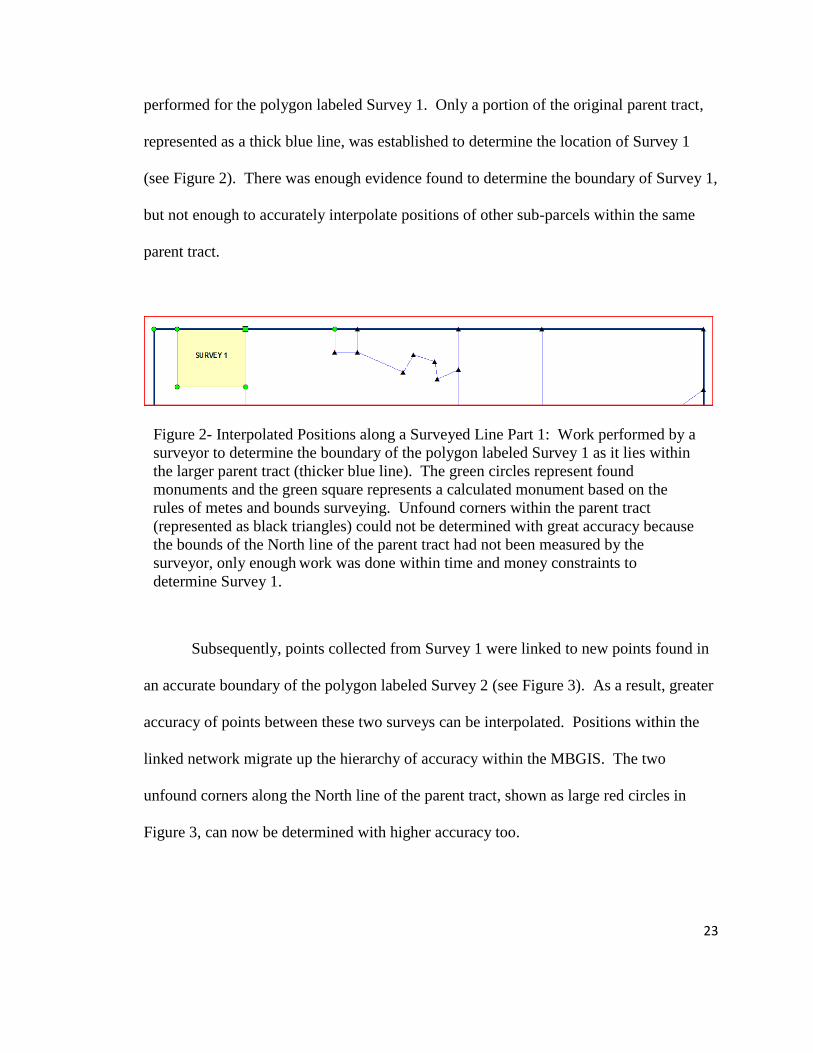
performed for the polygon labeled Survey 1. Only a portion of the original parent tract,
represented as a thick blue line, was established to determine the location of Survey 1
(see Figure 2). There was enough evidence found to determine the boundary of Survey 1,
but not enough to accurately interpolate positions of other sub-parcels within the same
parent tract.
Subsequently, points collected from Survey 1 were linked to new points found in
an accurate boundary of the polygon labeled Survey 2 (see Figure 3). As a result, greater
accuracy of points between these two surveys can be interpolated. Positions within the
linked network migrate up the hierarchy of accuracy within the MBGIS. The two
unfound corners along the North line of the parent tract, shown as large red circles in
Figure 3, can now be determined with higher accuracy too.
Figure 2- Interpolated Positions along a Surveyed Line Part 1: Work performed by a
surveyor to determine the boundary of the polygon labeled Survey 1 as it lies within
the larger parent tract (thicker blue line). The green circles represent found
monuments and the green square represents a calculated monument based on the
rules of metes and bounds surveying. Unfound corners within the parent tract
(represented as black triangles) could not be determined with great accuracy because
the bounds of the North line of the parent tract had not been measured by the
surveyor, only enough work was done within time and money constraints to
determine Survey 1.

24
Because original measurements are presumed accessible in a MBGIS, it is
possible to analyze the original positions measured in Survey 1 in terms of their
relationship to positions measured in Survey 2, and how both sets of points relate to
control points to further determine error within the system. The subsequent update of
measured positions would result not only in interpolated positions gaining accuracy, but
also originally measured positions being upgraded.
3.4 A Conceptual Model for Measurement Adjustment
The role of a surveyor has always been to accurately assess the boundary of the
property being surveyed (Robillard et al., 2003). This is done by establishing and
weighting the relationships between found and measured monuments in the field. A
MBGIS to manage metes and bounds survey data must also contain methods of storing
and weighting these relationships. Sections 3.1 through 3.3 above discussed
characteristics of metes and bounds data that must be represented in a MBGIS and the
use of absolute positioning of control points to establish a geodetic hierarchy of precision
Figure 3 - Interpolated Positions along a Surveyed Line Part 2: The upgradeable
accuracy of a MBGIS based on measured survey data and linking measured positions
through a control network. Monuments found from Survey 1 were linked with
monuments found for Survey 2 through common control points. As result, measured
accuracies between the found monuments were upgraded as well as any interpolated
position along the North line of the original parent tract. The red circles are still
unfound corners, but can be interpolated with higher precision because of the linked
measurements.

25
within a system of related data. This section integrates the parts by defining the required
relationships between different measurement classes using only measured angles and
distances to describe their relationship, thus creating a relational hierarchy.
Figure 4 below displays the relationships between the different measurement
classes that establish the hierarchy within a MBGIS. Control Points (CP) are grouped in
their own class and contain coordinates (x, y, and z) that are (assumed to be) absolute.
The Survey Points (SP) class contains points that are precisely measured or
referenced in legal descriptions by other surveyors, such as property corners or street
right-of-way monuments, and are used in the least-squares adjustment process. Because
not all points in the SP are established with an equal amount of accuracy, an Accuracy
attribute is used to weight measured points within the least-squares adjustment. This
value ranks the relative accuracies of various surveying techniques. For example, a
typical boundary survey might be assigned an accuracy value of 4 while a real-time
kinematic (RTK) survey might be assigned a value of 2. These rank values could be
provided in a reference table or a database domain.
A Data Source attribute of the SP also contributes to the weighting of points in the
error adjustment process. This attribute ranks the confidence held in the accuracy of the
data based on its source. For example, this can be used to indicate lower confidence in
certain surveyors’ measurements or uncertainty caused by missing metadata normally
provided within a legal description or survey plat of a tract of land. Although this type of
weighting is highly subjective, it must be included in a metes and bounds MBGIS
because it is important to assess the existence of certain vital items such as bearing basis
26
and scale factor that are frequently not reported by surveyors. A reference table or
database domain can be populated over time to record the ranks assessed for specific
sources and issues.
The relationship between pre-established control points and subsequent measured
points is defined by an angle (usually azimuth angle in surveyors’ raw data reports) and a
distance. These two attributes can be calculated between any two points in a system of
linked objects thus creating a lineage of measured relationships, creating a method in
which points in the SP are adjusted in relation to their lineage with points in the CP. The
lineage of the SP back to the CP is established by the Lineage relationship table, where a
PointID is matched with a ControlID and their relative angle and distance is recorded.
Each point in the CP can be related to one or more points in the SP and each point in the
SP may be related to one or more points in the CP, but not all points in the SP will be
directly related to points in the CP.
The Survey Points Association relationship table (SPA) retains measured angles
and distances between points in the SP class. The difference in the SPA and the Lineage
tables is that the former strictly interrelates survey points among themselves, without
reference to any absolute coordinate in the CP. The angles and distances in these
relationships are weighted through the attributes of the participating SP class and the
weighting is used in the error adjustment process.

27
MBGIS Relationship Hierarchy for Land Survey Data
The PointGroup table identifies redundant measurements in the SP class. The
result of each least-squares adjustment is a single point that represents the best fit of
redundant angles and distances. The PointGroup table contains descriptive information
Figure 4 – MBGIS Relationship Hierarchy for Land Survey Data: Relationships between
measured points and adjustments within a network would be achieved in a MBGIS using
the measured angles and distances between points. Measured Points are weighted in
terms of their accuracy and data source, and are adjusted based on their most likely
position relative to control points. Obviously more accurate points within a system
results in more accuracy overall within the network
MBGIS Relationship Hierarchy
28
about each single point that is represented redundantly in the dataset and links to the
relevant SPs through GroupID.
Finally, the Side Tie Points (STP) class contains all other points within the
MBGIS that are relative to the surveying environment, but not used in the least-squares
adjustment process. Points in the STP include items such as house corners, fences, and
driveways. The STP shares a Lineage relationship table with the SP in the same fashion
the SP and CP share a lineage, where points in the STP adjust based on their angular and
distance relationship to points in the SP in which a lineage is shared.
The relationships, classes and attributes shown in Figure 4 contain the elements
necessary to execute a least-squares adjustment of measured points in space and give the
surveyor the ability to retain the original measured positions. Neither of these
characteristics, both of which are essential to building and managing a metes and bounds
network, can be achieved in a traditional coordinate-based GIS (Goodchild, 2002). The
least-squares adjustment would use angles and distances between the CP and SP stored in
the Lineage relationship table, and relationships established by the SPA, to determine the
most likely angle and distance between all points in space. The Accuracy and
DataSource attributes within the SP weight each individual measurement within each
PointGroup. Points in the SP with higher accuracy are weighted higher and therefore
adjust less. Upgradeable accuracy would occur as more points are added to both the SP
and CP classes and linked to the system.

29
Chapter 4: Esri’s ArcGIS Parcel Fabric
The section above discussed elements of metes and bounds survey data within the
theory of a MBGIS–as points in space interrelated by angles and distances between other
points with some points having higher accuracy weight than others. The validity of a
survey in a metes and bounds system is contingent upon the verification of angles and
distances between monuments using ground measurements. Once again system is
singular as the goal of a MBGIS is to integrate all possible measurements into one
network (Buyong et al., 1991), a difficult concept when working with metes and bounds
survey data.
Measurement-based systems have already been established within other
computing environments such as CAD (Sipes, 2006). The advantage of a MBGIS over
other systems is the ability to harness the attributes of traditional GIS functionality while
still retaining original measurements for error adjustment, upgradable accuracy, and
particularly reuse in the field. Esri has attempted to achieve these benefits with their
release of ArcGIS 10 and the parcel fabric data model (Esri, 2012).
In this section, the Parcel Fabric data model is discussed as a “best practice” in
terms of employing the measurements of survey data within a GIS environment. Since
the Parcel Fabric data model is so extensive, only the parts pertaining to managing survey
data and retaining measurements are discussed below.
4.1 Measurement Elements of the Parcel Fabric
The parcel fabric data model is a conceptual framework of the components of a
parcel fabric dataset. The data model provides a schema for the creation of a geodatabase

30
containing the various feature classes and relationships used to store information about
parcel fabrics. The individual feature classes within a parcel fabric dataset are called
parcel fabric layers. The parcel fabric data model contains several elements that relate to
the measurement and error adjustment process. The phrase describing each element
below was taken directly from Esri’s web page describing the parcel fabric.2
1. Parcel lines, which store and preserve recorded boundary dimensions from legal
descriptions and other data sources
For a surveyor, these data include lines imported from a CAD environment or
legal descriptions involved in a deed sketch of an area surrounding a land survey
performed by the surveyor. The parcel lines retain the original or published measured
angles and distances between vertices. The retention of original measurements is key
within a MBGIS, but it is also significant to note that these original ground measurements
always remain unchanged, even after adjustment processes are applied.
A subtype of parcel lines is connection lines, which allow the user to integrate
additional ground measurements into the parcel fabric. Connection lines connect points
between parcels that are not adjacent. There are often times when legal descriptions
reference a bearing and distance to another monument or property corner that is not
adjacent to the tract of land (Robillard et al., 2006). This ground measurement can be
retained in the parcel fabric through the use of connection lines. Figure 5 displays a
connection line shown on a survey plat.
2Source:
http://help.arcgis.com/en/arcgisdesktop/10.0/help/index.html#/What_is_a_parcel_fabric/008500000002000000/

31
Figure 5 – Connection Lines: The arrow points to an additional measurement that
is not part of the boundary being surveyed, but displays an angle and distance
measured to a significant point within a metes and bounds system. A surveyor
could insert a connection line in the parcel fabric to represent this additional
measurement in order to integrate more ground measurements into the system.

32
2. Parcel points, which store x,y,z coordinates derived from a least-squares adjustment
Although these points are coordinate based, they represent the resulting corners
after a least-squares adjustment has been performed. If geometric continuity between
control points and survey data is strong, these parcel points represent an upgraded
location of the original measured points, and upgrade the accuracy of interpolating
unmeasured points.
3. Parcel polygons, defined by parcel lines
These polygons are the representation of the parcel lines after being imported into
the coordinate system and assembled as closed shapes. The polygons can store some
different measurement information such as misclosure ratio and the rotation and scale at
which the parcel was amended to fit into the coordinate network.
4. Line points, which are parcel corner points that lie on the boundaries of adjacent
parcels
In the surveying community, line points would be known as calculated points
along a known straight line when measured monuments or legal descriptions in a deed
sketch do not lie in a straight line (Robillard et al., 2003).
5. Control points, which have accurate, published coordinates for a physical location
The use of control points in a MBGIS was discussed above. In terms of the parcel
fabric, control points are always tied to a parcel corner point giving them an absolute
location. In terms of a MBGIS surveying environment, control points are accurately
located within the system and ordained to be absolute. The term fabric in parcel fabric is
indeed a metaphor for the manner in which the points, lines and polygons of the feature

33
class interact with each other. Control points in the parcel fabric are best described as the
points at which the fabric is “pinned” down (Esri, 2012) and cannot deviate from that
position. All positions between control points can still be molded and adjusted, but
control point coordinates are absolute.
6. Plans (table), which store information about the record of survey
The weighting procedure of measured positions is stored in the plans table. Each
plan is prescribed an accuracy attribute, the default being categories 1 (highest accuracy)
to 7 (lowest accuracy). The different accuracy ratings participate as weighting methods
within the least-squares adjustment process of the network. Each parcel and parcel line is
drawn or constructed within a plan thus giving that parcel and its lines a certain accuracy
weight for the least-squares adjustment. A plan may encompass the survey of a single
parcel or of many associated parcels completed in a single survey project.
7. Accuracies (table), which weight parcels in the least-squares adjustment
Known accuracies about each element of the parcel fabric is stored in this table
and accessed by the least-squares adjustment of the network. Although the default
accuracies were used for this research, they can be customized. Table 1 displays the
details of the different accuracy categories that can be assigned to each parcel in the
fabric dataset. The least-squares adjustment process uses these survey-style accuracy
thresholds when assigning weights to each parcel category. Standard deviation indicates
precision, or the spread of values when measuring the same target, whereas part per
million (PPM) is a measure of change or uncertainty in measurements and indicates
accuracy. The default levels 4 and 5 in the table contain the same PPM threshold but

34
different standard deviations indicating level 4 Accuracy measurements in the default
settings contain more precise but not necessarily more accurate measurements than
level 5 Accuracy measurements. The Description column shows the time period when
this level of accuracy was the best that could be achieved and it is used as one means of
assigning an accuracy level if no other information is available.
Table 1 - Parcel Fabric Accuracy Table: This table was taken from the ArcGIS 10.0 Help
Desktop Menu and displays the default settings for each accuracy category.
Source: http://help.arcgis.com/en/arcgisdesktop/10.0/help/index.html#//001t00000145000000.htm
8. Adjustment vectors (table), which store sets of displacement vectors from least-squares
adjustments
The adjustment vectors are an integral part of the parcel fabric and also important
within a MBGIS. This table stores the necessary information to adjust feature classes
related to the parcel fabric. For example, an access easement can be related to a parcel
line as being offset sixty feet and parallel to that line. Therefore, if the parcel line is
altered during the least-squares adjustment process, the adjustment vector table stores the
Accuracy
level
Std. deviation
bearing (secs)
Std. deviation
distance (m/ft)
PPM (m) (parts
per million) Description
1 5 0.001/0.00328 5 Highest
2 30 0.01/0.0328 25 After 1980
3 60 0.02/0.0656 50 1908–1980
4 120 0.05/0.164 125 1881–1907
5 300 0.2/0.656 125 Before 1881
6 3,600 1/3.28 1,000 1800
7 6,000 10/32.8 5,000 Lowest—excluded from
adjustment

35
necessary information to update the access easement, ensuring data integrity through the
measurement-based relationship (Goodchild, 2002).
Figure 6, from Esri’s Desktop Help Web page, describes the relationships
between the many parts mentioned above that form the parcel fabric data model.
Because the fabric retains original measurements, contains methods to adjust error and
improve accuracy, and stores a design to interpolate related features as a result of
adjusted positions, one may call it a measurement-based system. Figure 6 illustrates all
the parts that store measured data (Lines, Control, and Line Points) and the relationships
modeled to weight and execute the error adjustment process within the parcel fabric.
Figure 6 - Parcel Fabric Data Model: This UML diagram from Esri’s ArcGIS
documentation displays the relationships between the many parts that make up the
parcel fabric. Source: http://help.arcgis.com/en/arcgisdesktop/10.0/help/index.html#/The_parcel_data_model_in_the_parcel_fabric/008500000003000000/

36
4.2 Examples of Measurement Elements
The elements described above create the framework within the parcel fabric that
retain original measurements and drive the least-squares adjustment process, both of
which must exist to successfully manage metes and bounds survey data within a MBGIS.
This section provides practical demonstrations of how survey data is initially integrated
into the parcel fabric, how additional survey data is added, and the effect it has on the
management of the parcel fabric as a MBGIS.
4.2.1 Integrating Survey Data
A CAD dataset of survey data obtained in Hunt County, Texas, containing a
network of several surveyed points shown in Figure 7, was initially input into the parcel
fabric. The original data was gathered in the field using an assumed coordinate system
where the original point established in space was given an <x, y, z> ground coordinate of
<5000, 5000, 100>, respectively.
Because survey data must state the basis of bearing for a particular project, the
points in this dataset were rotated to the State Highway shown in the northerly portion of
Figure 7. The highway plans were designed and platted using a State Plane bearing
reference. This meant that the CAD dataset, although rotated to a different bearing basis
than originally collected in the field, still retained relative angles and distances between
other measured points collected in the field, but was merely rotated – not scaled into a
grid coordinate system – to match the highway plans. This also meant that one could
overlay the CAD dataset onto aerial imagery that was rectified using State Plane
coordinates consistent with the highway.

37
To ensure data was imported correctly and affirm the original measurements were
stored in the right fields designated in the Parcel Fabric data model, instructions on how
to import a CAD dataset provided in Esri’s “Loading Data into a Parcel Fabric” white
paper were followed carefully. A requirement of importing the CAD dataset was to
declare a coordinate system for the data. State Plane North Central Texas Zone (U.S.
Survey Feet) was chosen. The “Load a Topology into a Parcel Fabric” tool was then
used to load the line and parcels created from the CAD dataset.
Figure 7 - Initial CAD Import: These are the original lines and points imported into the
study area created in a CAD environment. This data was retrieved from Stovall and
Associates, Inc., a land surveying and mapping firm in Greenville, Hunt County, Texas.
It displays property lines determined by points measured in the field. All red lines in the
image are coded to be correct in terms of their measured positions and their relationship
to adjoining tracts of land. The red lines were imported into the study area data model
and given the highest accuracy rating.

38
4.2.2 Establishing Control Points
To simulate the collection of GPS points in the field, appropriate control points
were created manually so that data would be similar to that produced by a ground survey
in the field using GPS. Such control points produce geometric unity for better error
adjustment. Several control points were created at the location of different surveyed
parcel corners in the system. These became the absolute positional coordinates from
which least-squares adjustment was initiated and the fabric was “pinned” to the canvas.
Connection lines were also established across a State Highway dividing some of the
parcels. Since State right-of-way is considered the senior tract in relationship to
adjoining parcels, maintaining right-of-way width is important to producing an accurate
system. The connection lines were given the ground-measured width as indicated by the
distances displayed on the State right-of-way map. Figure 8 displays the connection lines
created across the right-of-way in the study area.
Figure 8 - Connection Lines within the Study Area: The blue lines are connection
lines drawn across highway right-of-way that ensure the ground-measured width of
the right-of-way during the adjustment process.

39
An initial least-squares adjustment was compiled to test the continuity of the
survey dataset and the control network. Its results proved to be a positive fit of data and
resulting coordinate shifts in parcel corner points were minimal. However, the slight
coordinate shifts did indicate some error between measured positions that had been
adjusted. The error was within survey measurement tolerances, but the shift was still
noted. The resulting file of the first least-squares adjustment is presented in the
Appendix.
An additional test within the study was undertaken to illustrate coordinate shifts
of parcel corner points when they are tied to a control point. The system assumes that a
control point has an absolute location of the point in space. This assumption is based
upon the method of establishment of control points. As mentioned above, control points
must be the most accurately established points within the coordinate dataset.
A control point in the system was given a slightly different coordinate than that of
its corresponding parcel corner point as shown by the image on the left in Figure 9. Once
the least-squares adjustment process was performed on the network, the parcel corner
point shifted in line with the control point, since they were intended to be at the same
position in space. The image on the right in Figure 9 displays the results of the
adjustment.

40
Figure 9 - Parcel Coordinate Shifts: The two images above display the parcel layer
and the parcel point that is coincident with a corresponding control point. In the right
image the parcel is shifted after a least-squares adjustment. The original coordinates
for each point differed slightly before the adjustment and were identical afterward.
This test illustrates the use of control points within a surveying network. When
certain property corners are be established using “control point” accuracy, they become
absolute positions in space relative to other unmeasured positions. When lines between
control points are original tract lines being surveyed, one may see the benefit of
“pinning” the endpoints resulting in points along that line being established with greater
precision.
4.2.3 Adding Parcels
Parcels can be added to the fabric using several methods. The three most popular
methods are:
Adding CAD data, as was the case for the initial setup of the study area.
Using coordinate geometry (COGO) tools within the parcel fabric to input a
written legal description which is illustrated below.
Digitization based on aerial imagery or other reference data.

41
The final method was not used in this study because this research is intended to
demonstrate methods in which land surveyors could input metes and bounds data into a
MBGIS and retain a reliable system. Parcel digitization would not fall within accuracy
thresholds desired by surveyors.
Parcels were added to the network in an attempt to display the use of error
adjustment within the network for increased accuracy when interpolating between
measured positions. Figure 10 is an image of the study area after the new parcels were
added using the parcel fabric COGO tools in accordance to their legal descriptions listed
in the most recent deed of the property filed at the Hunt County Courthouse. Three
parcels were initially created, according to their legal description, to fill a large hole in
the original fabric. They were given a different weight from that of the original parcels in
the fabric, using only the estimated date of the legal description as a factor (the default
setting in the parcel fabric).
When a parcel is added to the fabric, its initial starting point is assumed to be in a
local coordinate system and given a northing and easting of <0,0>. The ground
dimensions are used to input internal angles of the property and a Bowditch adjustment3
is used to calculate and correct any misclosure between the start and end point of the
traverse. At this time, the parcel is considered unjoined to the fabric and is represented in
its raw measurement form.
3 The Bowditch rule, also known as the compass rule, is a simple adjustment method that amends angular
error by proportionately distributing blunders based upon the length of lines or courses in a traverse versus the overall perimeter of the traverse (Mikhail & Gracie, 1981).

42
Figure 10 - Adding Parcels: The three parcels were added to the middle of the study area
using COGO tools provided within the parcel fabric toolset. A least-squares adjustment
was once again performed on the entire study area with favorable results.
The unjoined parcel is then linked to parcels in the fabric through shared points.
A Helmert transformation4 is used (rotation, scale, shift in x, shift in y) to determine the
location and representation of the parcel in the fabric. A local least-sqaures adjustment is
performed when the user defines more than two links when joining a parcel to the fabric.
The Helmert parameters at which the joined parcel fits is stored within the parcel polygon
attributes and is used in the bearing equation of the least-squares adjustment.
Once again a least-squares adjustment was performed on the data using the same
control points initially established. The result was an additional coordinate shift, but still
4 The Helmert transformation is a seven parameter transformation that preserves shape, while adjusting
scale, rotation of x, y, and z, and position of x, y, and z, when translating coordinates between two Euclidean spaces (Esri, 2012).

43
within the default constraints of the test. These three parcels integrated into the network
with little resistance and little coordinate shift, suggesting a decent fit of data. The results
of the least-squares adjustment can be seen in the Appendix.
4.2.4 Failed Adjustment
Two additional parcels were added to the fabric using the same COGO method as
was used for the three above. These two parcels were connected to the study area, but
altered the geometric unity of the test site. Figure 11 displays the elongated shapes of the
new parcels along the southern edge. Once again a least-squares adjustment was
performed on the entire study area; however, the adjustment failed. The failure was due
to several parcel lines exceeding the computed-minus-observed (c-o) distance threshold.
Figure 11 Failed Adjustment: The two odd-shaped parcels added at the bottom of
the study area caused several parcel lines to exceed the computed-minus-
observed distance tolerance for adjustment, which in turn caused the least-squares
adjustment to fail.

44
The ‘c-o’ computation is the difference between the newly computed coordinate parcel
line and the original ground distance or bearing attributes of the line.
There are two possible reasons for failure. The first is the lack of ‘geometric
unity’ within the system. As different shaped parcels are integrated into the fabric,
translation, rotation and scaling of each new parcel becomes difficult without additonal
measured positions on adjacent parcels. More redundancy with lines and points adjacent
to the odd-shaped parcel could have resulted in a successful adjustment.
The second reason for failure deals with the issue of ‘bearing basis’ in metes and
bounds surveying. As stated, surveyors establish their own compass bearing in a metes
and bounds system (Robillard et al., 2006). At times some legal descriptions are far from
true north orientation as the parcels are situated in fabric. When this occurs, the ‘c-o’
bearing threshold could cause the adjustment to fail. This failure occurs frequently in a
metes and bounds system, where every legal description in an area could have a different
‘bearing basis.’
A possible method to correcting failure due to multiple ‘bearing bases’ is to
sketch the original metes and bounds description in another layer using coordinate
geometry (COGO) tools. This newly drawn tract of land can then be translated and
rotated where it seems to fit in the fabric better. This approach orients the original
bearings closer to the fabric rotation. The original bearing is not as critical as retaining
original relative angle and distance in metes and bounds as mentioned above because the
surveyed line is the line between the two monumented corners at the surveyor’s defined

45
bearing (Robillard et al., 2003). The new rotated bearings can then be used to input the
new parcel into the fabric possibly resulting in a successful adjustment of the entire area.
4.2.5 Additional Test
If more time had been available to complete this study, field work would have
been performed to locate (with survey-grade accuracy) the property corners of the three
legal descriptions input into the system in relationship to the location of the published
control points in the system. Then the resulting error between the field measured location
and the interpolated position in the parcel fabric would be an indicator of how well the
least-squares adjustment was able to correct error in the network and estimate unknown
positions with greater accuracy based on the measurements already present in the system.
Furthermore, if the new surveyed positions were then added to the network, and
additional parcels were added per their legal descriptions, one could test to see if the
interpolated positions of these parcels contained less error than the first set, as the theory
of a MBGIS indicates they should.

46
Chapter 5: Towards the Management of Metes and Bounds Data in the
Parcel Fabric
The Esri parcel fabric data model is associated with several tools and attributes
for storing and utilizing original ground measurements (Esri, 2011). These are the
measurements used by land surveyors to solve property boundaries and determine
property corners. Because such a system retains and uses original measurements to
calculate error between measurements and to determine interpolated positions, one could
call it a MBGIS. However, as illustrated in the previous section, there must be certain
methodologies practiced in order for one to successfully integrate and manage metes and
bounds data with the parcel fabric. This section uses the results of the demonstrations of
integrating survey data described above to formulate a protocol to successfully manage
metes and bounds survey data using the parcel fabric.
The goal of the surveyor working in the parcel fabric would be to create a
seamless network of all his measured points within a service area (city, county, region,
etc.). The surveyor’s field measured data would be input with the highest accuracy rating
in the fabric, as it was all gathered, verified and linked through field measurements and
attributes about the measurements are known. Therefore it is the most reliable data
within the system.
Other parcels within the network might be given lesser accuracy ratings depending upon
the surveyor’s assessment of their accuracy. Although the survey date is the default
constraint within the accuracy table, other considerations are possible. For example, as
noted earlier, more or less weight might be placed on work performed by a particular
surveyor in the area because of personal knowledge of that surveyor’s work quality.

47
Thus, even though a surveyor’s legal description and survey was performed within the
accuracy-level two rating based on time frame, for example, it might be downgraded to
accuracy-level three or four.
The goal of the network from a surveying perspective is to interpolate
unmeasured property corners as precisely as possible before field crews begin their work
on a property. Land surveyors must always attempt to verify property corners in the field
(Robillard et al., 2003), a practice that will never be eliminated from surveying. But
giving field crews smaller zones in which to look for and identify monuments as property
corners can help save time in the field. These monuments can then be measured and their
subsequent parcels can then be upgraded to the highest accuracy parcel rating within the
fabric.
Control points within a metes and bounds system are irregular in contrast to the
systematic nature of the PLSS (Zimmer & Kirkpatrick, 2009). Control points would have
to be created by the private surveyor and be well positioned in terms of geometric
proportionality. It is evident through the demonstrations above that least-squares
adjustments have bearing and distance thresholds in terms of their benefit on the system
as a whole. It is more difficult to perform and analyze reliable adjustments to larger areas
of metes and bounds tracts. Since control points are “pinned” positions within a system,
one could systematically establish these points to regionalize a service area into several
different adjustment zones. Neighboring adjustment zones would share common control
points for their own adjustment of parcels within their region. The user would still
integrate all of their data into one network, but only employ certain control points in user-
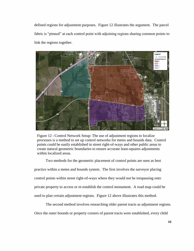
48
defined regions for adjustment purposes. Figure 12 illustrates the argument. The parcel
fabric is “pinned” at each control point with adjoining regions sharing common points to
link the regions together.
Two methods for the geometric placement of control points are seen as best
practice within a metes and bounds system. The first involves the surveyor placing
control points within street right-of-ways where they would not be trespassing onto
private property to access or re-establish the control monument. A road map could be
used to plan certain adjustment regions. Figure 12 above illustrates this method.
The second method involves researching older parent tracts as adjustment regions.
Once the outer bounds or property corners of parent tracts were established, every child
Figure 12 - Control Network Setup: The use of adjustment regions to localize
processes is a method to set up control networks for metes and bounds data. Control
points could be easily established in street right-of-ways and other public areas to
create natural geometric boundaries to ensure accurate least-squares adjustments
within localized areas.

49
parcel inside the original parent tract would be adjusted relative to the absolute position
of the parent tract. This second method, illustrated in Figure 13, could produce a true
surveying network of control and adjustment regions based upon the fundamental design
of a metes and bounds system, where smaller child tracts are formed relative to their
position of larger parent tracts.
Figure 13 - Parent Tract Adjustment Regions: This image displays three separate
parent tracts researched by the surveyor in order to determine least-squares
adjustment regions within the parcel fabric. Historical information about parent tracts
located in other layers within the MBGIS would match the control network
adjustment regions.
For the second method, historical research data, including parcel seniority rights,
could be stored in the GIS for later use. This approach would take significant planning
and time to establish, however. A survey company could begin with just one adjustment

50
region and slowly add additional regions, and/or integrate regions that are distant from
each other. Thus Control networks established using GPS would obviously be preferable
as integrating datasets would be of high accuracy-level.
Most elements of metes and bounds survey data can be accurately represented
within the parcel fabric. Original CAD data can be integrated into the fabric with the
ground measurements retained. The parcels can be assigned weights to justify their
existence within the parcel fabric. Control networks can be planned and established
using either natural boundaries for adjustment regions or historical tracts can be
researched to establish original parent tract adjustment regions. Knowledge of these
elements are important for surveyors to gain confidence in the use of the parcel fabric
both as a MBGIS and as a “best practice” method to manage survey data.
One final element to consider when adapting metes and bounds survey data to the
parcel fabric involves integrating or adding measured points into the fabric. Adding
measured positions from GPS would be the simplest method: these could be easily
integrated into the system and tied to a specified adjustment region. However, there are
times when the capabilities of the GPS are not available to complete ground
measurements and traditional surveying instruments must be used. Then, the surveyor
must tie into several control points or several common points already established in the
fabric. Tieing back to prior surveys not only allows additional redundancy for
measurement adjustment operations, but also ensures that new points are integrated into
the existing system accurately.

51
All positions collected in the field (either by GPS or by traditional surveying
equipment) would then be linked together in their specified adjustment region and given
the highest accuracy as all attributes about the points are known. Adjoining or un-
surveyed parcels could then be added per their legal descriptions and given an accuracy
rating as mentioned above. The fit of the data and results of adjustment operations would
indicate to the user the reliability of un-surveyed tracts of land. Ultimately, more points
gathered in the field would result in high accuracy survey regions and precise estimations
for interpolated positions. Correctly estimating interpolated positions could save
tremendous time in the field.

52
Chapter 6: Discussion
The parcel fabric data model contains several features that are indicative of a
measurement-based system. The lines within the model store original ground
measurements which are used in a least-squares adjustment process, where resulting
vector tables can be used to incrementally correct other features within the data model.
Resulting parcel corner point locations indicate a more accurate interpretation of how
properties are represented on the ground. However, there are several elements of the
parcel fabric that do not fit within the theory of a MBGIS. These elements are mentioned
below.
The irony of the parcel data model and using the parcel fabric is the first thing a
user must do is define a coordinate system (Esri, 2011). One could argue that ground
measurements are already compromised by this initial system definition and it is
impossible to correct or update parts of the system without creating geometric distortion
(Goodchild, 2002). This problem is evident within the least-squares adjustments on the
sample data and fabric adjustments demonstrated above. As more parcels were created
based upon their recorded legal descriptions, it became difficult to successfully complete
an adjustment in relation to the absolute coordinate location of control points within the
default thresholds of the adjustment process. The problem arises from the many different
bearing bases and distance factors used by land surveyors who have performed work in a
given area. These cannot all be adjusted relative to absolute positions while maintaining
the accuracy thresholds displayed in Table 1 above. Because of the unknowns within the
metes and bounds systems, the least-squares adjustment fails or topological distortions
53
are created if the adjustment tool thresholds are expanded. Therefore adjustments would
have to be constrained to very localized regions to ensure geometric unity.
A second survey-related issue arises from the use of a projected coordinate system
for the parcel fabric to represent tracts of land in space. The original theory of MBGIS
(Goodchild, 2002) as it relates to representing land surveying data describes a system
where all linked measurements contain the same spatial reference or the functions needed
to derive a common spatial reference and are scaled to ground measurements. Additional
measurements are then incrementally added to the system using the same survey
parameters (ground rotation and scale) thus allowing the original measurements to carry
the information needed to correct uncertainty (Buyong et al., 1991). This simplicity is
not possible within the parcel fabric feature class. Parcel lines store original ground
measurements which are used for adjustment purposes, but parcels are only linked
through the projected coordinates of parcel corner points.
There is also no method within the parcel fabric of calculating errors of original
measurements based on the addition of ground measurements to the network. This type
of calculation would give the user the ability to determine uncertainty in particular
measurements within the system (Goodchild, 2002). The only method of doing this in
the current parcel fabric involves the “guessing game” of a user-assigned accuracy level.
Instead the user must define the geometric boundaries and control network in which he
believes the least-squares adjustments will not fail or create topological distortions.
The parcel fabric also does not allow the transformation of parcel corner points
back to original ground measurements once they are in a projected coordinate system.

54
Some argue the optimal method of representing data is within a projected coordinate
system for data visualization and representation purposes (Jackson & Rambeau Sr.,
2007). However, a land surveyor must have the ability to use the coordinates derived in
the system on the ground to set new property corners and other monuments and to link
additional measurements. Since projections ultimately distort the geometry of the earth’s
surface, the use of displayed parcel corner coordinates would arguably be incorrect if
used to establish ground points.

55
Chapter 7: Conclusion
The goal of this research was to investigate and explore the management of metes
and bounds survey data integrated into a GIS. Traditional GIS practices and coordinate-
based systems are not ideal for the storage and retrieval of measurement-based survey
data. Rather if metes and bounds data is to be managed in a GIS environment, then the
system must be a MBGIS.
The retention and use of original measurements within a MBGIS for metes and
bounds survey data was theorized in Section 3 and relationships that must exist between
measured points were established. This proved that MBGIS provides a suitable format to
manage traditional metes and bounds survey data as well as modern data collected from
popular technologies such as GPS. A MBGIS for survey data would contain the
capabilities to:
Retain these original survey measurements to reuse in the field and to link to
additional points.
Apply metes and bounds surveying rules to determine a property boundary.
Assess unprojected error within the system for quality assurance purposes.
Skepticism of GIS within the surrveying community is a result of the traditional
practices of GIS (Deakin, 2008). Using a MBGIS to manage metes and bounds survey
data would produce less skepticism among surveyors. Esri’s ArcGIS 10 parcel fabric
data model was proposed as a “best practice” to manage metes and bounds survey data
within a GIS because it contains elements of a measurement-based system.

56
Section 4 illustrated several elements of the parcel fabric that incorporate original
ground measurements. To explore and test the measurement-based elements of the parcel
fabric, a CAD dataset was integrated into an empty parcel fabric model, then parcels were
added to the fabric and least-squares adjustments were applied. It was discovered that
original measurements stored within the fabric play a large role in the adjustment process
as well as accuracy weighting within the network.
These demonstrations indicate that the parcel fabric is suitable to manage metes
and bounds survey data. However, the surveyor creating the system would need to plan
adjustment zones appropriately in order for the parcel fabric to best utilize original
measurements. The surveyor would ultimately designate his own ground measurements
as the highest accuracy weight, while assigning different accuracy weights to other data
added to the fabric. Adjustments would then be more reliant upon ground measurements
taken by the surveyor and the geometry of the adjustment zones.
Managing survey data within a GIS environment would be beneficial to both the
GIS and surveying communities. Surveyors would obtain an ability to manage their data
in one system, while the GIS community would obtain the benefit of highly accurate data
managed by others. If the surveying community is to become less apprehensive to use
GIS to manage their data—especially when managing data in metes and bounds states
like Texas—knowledge of how measured positions are retained and utilized within a GIS
is necessary.
Esri’s parcel fabric does indeed contain most aspects of a measurement-based
system, and has the capabilities to manage metes and bounds survey data. However,

57
future work must be done to eliminate the drawbacks of the fabric model discovered in
this study, in particular: retaining measurements, applying survey rules, and assessing
unprojected error. For surveyors, having a MBGIS where error between original
measurements can be assessed and where groups of fitted coordinates can be transformed
back to their measurable locations on the ground is essential. The additions outlined here
would establish Esri’s parcel fabric as a MBGIS suitable for surveyors, even in metes and
bounds states such as Texas. This, in turn, would allow surveyors to integrate GIS
successfully into their business processes, providing tools to manage and retain their
original measurements on a long-term basis.

58
Glossary
Azimuth: Unit of angular measurement between two points determined by the number of
degrees from north measured from 0 to 359 rotating in a clockwise direction. North in
azimuth angle measurements can be magnetic or true north, or designated by the
surveyor.
Bearing: The horizontal angle that a line makes with the meridian of reference adjacent to
the quadrant in which the line lies. Bearings are classified according to the meridian of
reference, as: astronomic, geodetic, magnetic, grid, assumed, etc. A bearing is identified
by naming the end of the meridian from which it is reckoned, either north or south, and
the direction of that reckoning, either east or west. Thus, a line in the northeast quadrant
making an angle of 50 degrees from the reference meridian will have a bearing of N 50
degrees E.
Bearing Basis (Rotation, Control Line): The bearing between two points on a survey
which serves as the reference system for all other lines on the survey.
Call: Any single monument, landmark or measurement mentioned in a legal description.
For example, North 90 degrees east, 350 feet is a call, or East 6000 feet to a concrete
monument. A series of calls which begin and end in the same position form the legal
description of a property.
Child Tract: A tract of land (smaller than parent tracts) that were split from larger parent
tracts and sold.
Control Point: A point in space determined to be located with the greatest precision and
accuracy. Most control points in modern surveying are determined using RTK or
differentially corrected GPS technology.
Coordinate: A set of numbers (x, y, z) used in specifying the location of a point.
Coordinate Geometry: Also known as COGO, is an automated process to sketch legal
descriptions and other surveys using the angles, distances and monuments provided by
surveyors in their property descriptions.
Data Collector: A device used in the field while surveying that records and stores angles
and distances between objects located in the field that are pertinent to completing a
boundary survey.
Distance: The unit of measure, most commonly described in Texas in units of feet, used
in surveying to help describe the relationship between two points. In terms of land

59
surveying, distance is synonymous with slope distance, which is the calculated distance
between two points at different elevations. More traditional distance units of surveying
in Texas include the chain, link, Spanish vara, yard, and rod.
Evidence: Physical objects, monuments, traces of objects or any other object or
relationship discovered and measured in the field while performing a survey that aids in
correctly determining the metes and bounds of a parcel of land.
Ground Measurement: The actual measurement determined using surveying
instrumentation in the field where no scale factor or projection has been applied to the
measurement itself.
Junior Tract: The youngest of two or more adjacent survey whose angles, distances, and
monument calls are subordinate to tracts of land that are senior. Junior tracts are usually
the last child tracts split from a parent tract of land.
Metes and Bounds: A method of surveying in which a property is described by angles,
distances, and monuments on the ground (metes) in relationship to adjacent tracts
(bounds).
Monument: A permanently placed marking on the surface of or in the ground that is used
to represent a property corner of a parcel of land or some other important feature such as
a control point. These include iron re-bar sunken into the ground, concrete monuments, a
chiseled X or V in concrete, or a nail hammered into asphalt.
Parent Tract: A tract of land (usually quite large at one point in time) from which
additional ‘child tracts’ are split.
Raw Data: The original angles, distances, and descriptions of objects found in the field
while surveying, usually stored in a data collector in the field and downloaded to a
computer at the office. Raw data is used in most surveying software for error analysis
and adjustment.
Real Time Kinematic (RTK): A method of satellite navigation technology used in land
surveying where a single reference station (also known as a base station) provides real-
time corrections to a rover collecting positions, providing sub-centimeter accuracy
without post-processing.
Right-of-Way: The strip of land that determines the legal width of a road or railroad or
the width of a pipeline, power line, or telephone easement.

60
Scale Factor: The factor by which a set of measurements are multiplied to transform the
measurements into a projected plane or coordinate system.
Senior Tract: The eldest of two or more adjacent surveys whose angles, distances, and
monument calls take precedence over junior tracts. The most senior tract is usually the
first child tract split from a parent tract of land.

61
References
Buyong, T. B., Kuhn, W., & Frank, A. U. (1991). A Conceptual Model of Measurement-
Based Multipurpose Cadastral Systems. Journal of the Urban and Regional
Information Systems Association , 3 (2), 35-49.
Carlson. (2011). Carlson GIS. Retrieved December 3, 2011, from Carlson Software:
http://www.carlsonsw.com/PL_CS_GIS.html
Corbley, K. P. (2001). Land Information New Zealand Creates Online Title and Land
Survey Database. Retrieved October 3, 2011, from ArcNews Online:
http://www.esri.com/news/arcnews/winter0102articles/landinfo-newz.html
Deakin, A. K. (2008). Debating the Boundary between Geospatial Technology and
Licensed Land Surveying. Surveying and Land Information Science , 68 (1), 5-14.
Esri. (n.d.). ArcGIS Resource Center. Retrieved November 15, 2011, from Desktop 10:
http://help.arcgis.com/en/arcgisdesktop/10.0/help/index.html
Esri. (n.d.). GIS for Surveying. Retrieved October 20, 2011, from Esri:
http://www.esri.com/industries/surveying/
Esri. (2011). Loading Data into a Parcel Fabric. Redlands: Esri.
Felus, Y. A. (2007). Essential GIS Concepts in Surveying Education. Surveying and Land
Information Science , 67 (3), 175-182.
General Land Office of Texas. (2011). General Land Office of Texas. Retrieved
November 15, 2011, from The Land Office:
http://www.glo.texas.gov/GLO/index.html
Goodchild, M. (2002). Measurment-Based GIS. In P. F. Fisher, Spatial Data Quality (pp.
5-17). London: Taylor & Francis.
Greenfeld, J. P. (2008). Surveying Body of Knowledge--Preparing Professional
Surveyors for the 21st Century. Surveying and Land Information Science , 68 (3),
133-143.
Heo, J. (2004, February). Spatial and Temporal Functional Requirements for an Extended
Parcel-Based Land Information System. Journal of Surveying Engineering , 20-
28.

62
Jackson, J., & Rambeau Sr., R. (2007, June). Does GIS Help Surveyors Get the Job Done
Better and Faster? Professional Surveyor Magazine .
Jeffress, G. (2005). GIS and Surveying: Future Opportunities. Surveying and Land
Information Science , 65 (3), 169-177.
Jeffress, G. (2003). The Value of Cadastral Surveyiing to Efficient Land Administration.
Surveying and Land Information Science , 63 (4), 253-258.
Mikhail, E. M., & Gracie, G. (1981). Analysis and Adjustment of Survey Measurements.
New York, New York, U.S.: Van Nostrand Reinhold Company, Inc.
Navratil, G., Franz, M., & Pontikakis, E. (2004). Measurement-Based GIS Revisited. 7th
AGILE Conference on Geographic Information Science (pp. 771-775). Heraklion:
Institute for Geoinformation.
Olaleye, J. B., Abiodun, O. E., Olusina, J. O., & Alademoni, A. S. (2011). Surveyors and
the Challenges of Digital Surveying and Mapping Technology. Surveying and
Land Information Science , 71 (1), 3-11.
P2 Energy Solutions. (2011). Tobin. Retrieved December 2, 2011, from Off the Shelf
Map Data: http://www.tobin.com/psMain.asp
Point of Beginning. (2010). POB Online. Retrieved December 7, 2011, from Point of
Beginning Home Page: http://www.pobonline.com/
Robillard, W. G., Wilson, D. A., & Brown, C. M. (2006). Evidence and Procedures for
Boundary Locations (5th ed.). Hoboken, New Jersey, U.S.: John Wiley & Sons,
Inc.
Robillard, W., Wilson, D., & Brown, C. (2003). Brown's Boundary Control and Legal
Principles (5th ed.). Hoboken, New Jersey, U.S.: John Wiley & Sons, Inc.
Rolbiecki, D. A., & Lyle, S. D. (2008). Hybrid State Plane Coordinate System for
Transforming A City Wide Survey Control Network to Surface Values: Case
Study for Frisco, Texas. Journal of Surveying and Engiineering , 106-114.
Sipes, J. L. (2006). Integrating CAD and GIS. CADalyst , pp. 48-50.
Sorensen, M., & Wetzel, R. (2007). GIS the Survey Way. Professional Surveyor
Magazine .

63
Stamper, F. A. (1983). A Handbook for Texas Abstracters and Title Men (2nd Edition
ed.). Austin, Texas, U.S.: Texas Land Title Association as Assignee of Primitive
Press.
The American Surveyor. (2011). American Surveyor Publications Archives. Retrieved
December 7, 2011, from American Surveyor Magazine:
http://www.amerisurv.com/content/category/18/335/153
U.S. Department of the Interior, Bureau of Land Management. (1973). Manual of
Surveying Instruction. (R. Minnick, Ed.) Washington D.C.: Landmark Enterprise.
Wurm, K. (2007). An Assessment of the Upgradable Spatial Accuracy of the Geographic
Coordinat Data Base. Surveying and Land Information Science , 67 (2), 87-90.
Wurm, K., & Hintz, R. J. (2003). Use of Source Identification in the Optimization of a
Measurement-based Land Information System. Surveying and Land Information
Science , 63 (1), 55-61.
Zimmer, R. (2011). Convert CAD Data to GIS. The American Surveyor , 8 (1), pp. 28-38.
Zimmer, R., & Kirkpatrick, S. (2009). GIS Data Integration with the GCDB. The
American Surveyor .

64
Appendix: Least-Squares Adjustment Results
The data below are the results of the three least-squares adjustments generated by
ArcGIS in a temporary text file. The data in the text file was copied and pasted to this
appendix. They show whether the adjustment was completed or if it failed. The first set
of results is from the initial least-squares adjustment. The second set shows the results
after three parcels were added, and the third set is from the failed adjustment. Each set
contains different error residuals and additional statistics about the adjustment process
that indicate to the user if how the parcels were adjusted in space.
Initial Least-squares Adjustment
Craig Bartosh: USC Spatial Sciences Adjustment of Parcels Page: 1
Parcel Editor
ADJUSTMENT COMPLETED
Adjustment Settings
=======================
Linear Units : Foot_US
Coordinate System: NAD_1983_StatePlane_Texas_North_Central_FIPS_4202_Feet
No height data, assuming parcels are at sea level
Check Tolerances:
Bearings 1°40'00"
Distances 0.33
Dependent lines : No
Historical Data : Yes
Fixed Boundary : No
Results File : C:\Users\CBARTO~1\AppData\Local\Temp\FabricAdjustmentReport.lst
Adjustment Statistical Summary
==============================
Number of Control Points = 9
Number of Parcels = 31
Number of Points = 77
Number of Bearings = 170
Number of Distances = 170
Number of Unknowns = 167
Redundancy = 173
Bearings Exceeding Tolerance = 0
Distances Exceeding Tolerance = 4
Close Points Found = 0
Line Point Errors Found = 0

65
Max. coordinate shift: Easting = -0.000, Northing = 0.000 at point 119
Average coordinate shift: Easting = -0.000, Northing= -0.000
Mean(average) of coordinate residuals = 0.01
Standard deviation of coordinate residuals = 0.05
Range of coordinate residuals = 0.22
Close Points Report: Tolerance = 0.656
===================
0 close points found.
Linepoints Report: Tolerance = 0.656
===================
0 Linepoints found outside of the Check Tolerance
Parcel Lines Report - Difference between Computed and Observed/Recorded (c-o)
============
1/ModernSurveys Line: 68-71 Distance(c-o)=0.365
TAParcels_483/<map> Line: 64-68 Distance(c-o)=0.548
TAParcels_483/<map> Line: 68-71 Distance(c-o)=0.365
TAParcels_483/<map> Line: 71-70 Distance(c-o)=0.334
Suspect Points and Lines (exceeds 3x std deviation of adjusted data)
========================
Plan/Parcel Parcel Misclose Point dx dy
<map>/TAParcels_483 0.000 0.001 64 0.056 0.016
Plan/Parcel Parcel misclose From To Length (c-o)
StovallSurvey/TAParcels_479 -0.001 0.000 53 52 665.970 0.085
<map>/TAParcels_483 0.000 0.001 64 72 150.061 0.105
<map>/TAParcels_483 0.000 0.001 68 71 675.353 0.111
<map>/TAParcels_483 0.000 0.001 71 70 523.083 0.102
ModernSurveys/1 0.000 0.000 52 68 413.388 0.053
ModernSurveys/1 0.000 0.000 68 71 675.353 0.111
ModernSurveys/1 0.000 0.000 53 52 665.970 0.085
DigitizedParcels/NewParcel37 0.000 0.000 115 116 194.982 0.054
---------- Control Report ----------
TRANSFORMATION RESULTS
Point X Y dx dy Name
# 99 2687639.598 7071752.786 0.000 0.000 CP_99
# 6 2684056.023 7070223.857 0.000 0.000 CP_6
# 57 2683941.106 7067581.659 0.000 0.000 CP_57
# 89 2692458.541 7068600.426 0.000 0.000 CP_89
# 68 2688033.370 7068056.512 0.000 0.000 CP_68
# 70 2689743.861 7070288.805 0.000 0.000 CP_70
# 53 2686664.716 7070234.055 0.000 0.000 CP_53
# 52 2686677.131 7068049.154 0.000 0.000 CP_52

66
Least-Squares with three new Parcels
Craig Bartosh: USC Spatial Sciences Adjustment of Parcels Page: 1
Parcel Editor ADJUSTMENT COMPLETED
Adjustment Settings
=======================
Linear Units : Foot_US
Coordinate System: NAD_1983_StatePlane_Texas_North_Central_FIPS_4202_Feet
Check Tolerances:
Bearings 1°40'00"
Distances 0.33
Dependent lines : No
Historical Data : Yes
Fixed Boundary : No
Results File : C:\Users\CBARTO~1\AppData\Local\Temp\FabricAdjustmentReport.lst
Adjustment Statistical Summary
==============================
Number of Control Points = 6
Number of Parcels = 34
Number of Points = 91
Number of Bearings = 200
Number of Distances = 198
Number of Unknowns = 205
Redundancy = 193
Bearings Exceeding Tolerance = 0
Distances Exceeding Tolerance = 3
Close Points Found = 0
Line Point Errors Found = 0
Max. coordinate shift: Easting = 0.665, Northing = -0.495 at point 182
Average coordinate shift: Easting = -0.020, Northing= -0.014
Mean(average) of coordinate residuals = 0.01
Standard deviation of coordinate residuals = 0.16
Range of coordinate residuals = 0.78
Warning: Control point CP_53 references no point ID
Warning: Control point CP_52 references no point ID
Warning: Control point CP_68 references no point ID
Close Points Report: Tolerance = 0.656
===================
0 close points found.
Linepoints Report: Tolerance = 0.656
===================
0 Linepoints found outside of the Check Tolerance
Parcel Lines Report - Difference between Computed and Observed/Recorded (c-o)
============
1/ModernSurveys Line: 183-184 Distance(c-o)=0.776

67
1/OldSurveys Line: 129-128 Distance(c-o)=-0.490
1/OldSurveys Line: 128-129 Distance(c-o)=-0.490
Suspect Points and Lines (exceeds 3x std deviation of adjusted data)
========================
Plan/Parcel Parcel Misclose Point dx dy
OldSurveys/1 0.000 -0.000 183 0.100 -0.130
OldSurveys/1 0.000 -0.000 182 0.143 -0.121
OldSurveys/1 0.000 -0.000 181 0.151 -0.101
OldSurveys/1 0.000 -0.000 68 0.133 0.089
OldSurveys/1 0.000 -0.000 52 -0.145 0.061
OldSurveys/1 0.000 -0.000 53 -0.144 -0.055
Plan/Parcel Parcel misclose From To Length (c-o)
OldSurveys/1 0.000 -0.000 186 183 53.329 0.229
OldSurveys/1 0.000 -0.000 128 129 117.013 0.164
Error vectors between Inactive Control Points and Fabric points
========================================
Point Bearing Distance Name
0 N00°48'23E 7563489.730 CP_53
0 N00°48'45E 7561451.769 CP_52
0 N00°49'19E 7561940.641 CP_68
---------- Control Report ----------
TRANSFORMATION RESULTS
Point X Y dx dy Name
# 99 2687639.598 7071752.786 0.000 0.000 CP_99
# 6 2684056.023 7070223.857 0.000 -0.000 CP_6
# 57 2683941.106 7067581.659 -0.000 0.000 CP_57
# 89 2692458.541 7068600.426 0.000 -0.000 CP_89
# 70 2689743.861 7070288.805 -0.000 0.000 CP_70
# 90 2686918.470 7070386.530 -0.000 -0.000 CP_90

68
Failed Results
Craig Bartosh: USC Spatial Sciences Adjustment of Parcels Page: 1
Parcel Editor ADJUSTMENT FAILED
Close Points Report: Tolerance = 0.656
===================
0 close points found.
Linepoints Report: Tolerance = 0.656
===================
1/OldSurveys Line: 208-68 Linepoint=225, Offset= 5.638
1 Linepoints found outside of the Check Tolerance
Parcel Lines Report - Difference between Computed and Observed/Recorded (c-o)
============
TAParcels_489/StovallSurvey Line: 94-92 Distance(c-o)=0.456
## TAParcels_483/<map> Line: 64-68 Distance(c-o)=1.091
TAParcels_483/<map> Line: 71-70 Distance(c-o)=0.562
1/ModernSurveys Line: 194-195 Distance(c-o)=0.859
1/ModernSurveys Line: 196-190 Distance(c-o)=-0.429
## 1/ModernSurveys Line: 209-208 Distance(c-o)=8.297
1/ModernSurveys Line: 208-212 Distance(c-o)=-0.846
## 1/ModernSurveys Line: 212-209 Distance(c-o)=-5.563
1/OldSurveys Line: 198-196 Distance(c-o)=0.480
## 1/OldSurveys Line: 68-208 Distance(c-o)=-8.485
## 1/OldSurveys Line: 208-209 Distance(c-o)=8.836
1/OldSurveys Line: 225-68 Bearing(c-o)= 2°27'19", Effect=8.617
ERROR: Unable to complete adjustment. 5 parcel lines did not adjust within 3x the specified tolerances.