E.J. OpilaGlenn Research Center, Cleveland, Ohio

Integrated High Payoff Rocket PropulsionTechnology (IHPRPT) SiC Recession Model

NASA/TM—2009-215650

December 2009

https://ntrs.nasa.gov/search.jsp?R=20100002888 2020-04-08T21:25:51+00:00Z

NASA STI Program . . . in Profi le

Since its founding, NASA has been dedicated to the advancement of aeronautics and space science. The NASA Scientifi c and Technical Information (STI) program plays a key part in helping NASA maintain this important role.

The NASA STI Program operates under the auspices of the Agency Chief Information Offi cer. It collects, organizes, provides for archiving, and disseminates NASA’s STI. The NASA STI program provides access to the NASA Aeronautics and Space Database and its public interface, the NASA Technical Reports Server, thus providing one of the largest collections of aeronautical and space science STI in the world. Results are published in both non-NASA channels and by NASA in the NASA STI Report Series, which includes the following report types: • TECHNICAL PUBLICATION. Reports of

completed research or a major signifi cant phase of research that present the results of NASA programs and include extensive data or theoretical analysis. Includes compilations of signifi cant scientifi c and technical data and information deemed to be of continuing reference value. NASA counterpart of peer-reviewed formal professional papers but has less stringent limitations on manuscript length and extent of graphic presentations.

• TECHNICAL MEMORANDUM. Scientifi c

and technical fi ndings that are preliminary or of specialized interest, e.g., quick release reports, working papers, and bibliographies that contain minimal annotation. Does not contain extensive analysis.

• CONTRACTOR REPORT. Scientifi c and

technical fi ndings by NASA-sponsored contractors and grantees.

• CONFERENCE PUBLICATION. Collected papers from scientifi c and technical conferences, symposia, seminars, or other meetings sponsored or cosponsored by NASA.

• SPECIAL PUBLICATION. Scientifi c,

technical, or historical information from NASA programs, projects, and missions, often concerned with subjects having substantial public interest.

• TECHNICAL TRANSLATION. English-

language translations of foreign scientifi c and technical material pertinent to NASA’s mission.

Specialized services also include creating custom thesauri, building customized databases, organizing and publishing research results.

For more information about the NASA STI program, see the following:

• Access the NASA STI program home page at http://www.sti.nasa.gov

• E-mail your question via the Internet to help@

sti.nasa.gov • Fax your question to the NASA STI Help Desk

at 443–757–5803 • Telephone the NASA STI Help Desk at 443–757–5802 • Write to:

NASA Center for AeroSpace Information (CASI) 7115 Standard Drive Hanover, MD 21076–1320

E.J. OpilaGlenn Research Center, Cleveland, Ohio

Integrated High Payoff Rocket PropulsionTechnology (IHPRPT) SiC Recession Model

NASA/TM—2009-215650

December 2009

National Aeronautics andSpace Administration

Glenn Research CenterCleveland, Ohio 44135

Available from

NASA Center for Aerospace Information7115 Standard DriveHanover, MD 21076–1320

National Technical Information Service5285 Port Royal RoadSpringfi eld, VA 22161

Available electronically at http://gltrs.grc.nasa.gov

Level of Review: This material has been technically reviewed by technical management.

NASA/TM—2009-215650 iii

Contents 1.0  Summary .............................................................................................................................................. 1 2.0  SiC Recession Calculation Input Parameters and Data ........................................................................ 1 

2.1  Combustion Gas Chemistry ....................................................................................................... 1 2.2  SiC Material Temperature ......................................................................................................... 2 2.3  Combustion Gas Pressure and Velocity .................................................................................... 2 2.4  Thermochemical Data for Volatile Si-O-H Species .................................................................. 3 

3.0  Recession Calculations ......................................................................................................................... 4 3.1  Calculation of Volatile Species Partial Pressures ...................................................................... 4 3.2  Gas Boundary Limited Recession Calculation .......................................................................... 5 

4.0  Validation of the Recession Model ...................................................................................................... 7 4.1  Existence of a Silica Surface Layer on the SiC ......................................................................... 7 

4.1.1  FACTSAGE Calculations Indicate SiO2 is Present on the SiC Surface ....................... 8 4.1.2  Estimated Silica Thickness on SiC Surface From Rate Constants ............................... 8 4.1.3  Estimated Silica Thickness on SiC From EDS Measurements .................................... 9 4.1.4  Comparison of Cell 22 Conditions to Active Oxidation Conditions Reported in the

Literature ...................................................................................................................... 9 4.2  Gas Boundary Layer Limited Volatilization ........................................................................... 12 4.3  Evaluation of Thermochemical Data for Si-O-H(g) ................................................................ 13 

4.3.1  SiO(g) ......................................................................................................................... 13 4.3.2  Si(OH)4(g) .................................................................................................................. 13 4.3.3  SiO(OH)2(g) ............................................................................................................... 14 4.3.4  SiO(OH)(g) ................................................................................................................. 14 

5.0  Other Mechanisms Contributing to SiC Degradation in Addition to Silica Volatility ....................... 16 5.1  Cracking .................................................................................................................................. 17 5.2  Pitting ...................................................................................................................................... 17 5.3  Grooving .................................................................................................................................. 17 5.4  Oxidation of Underlying Carbon Fibers .................................................................................. 17 

6.0  Shear Flow of Liquid Layers at High Temperatures .......................................................................... 18 6.1  Modeling Shear Flow of Liquids ............................................................................................. 18 6.2  Comparison of Observed and Modeled Shear Flow of Liquids .............................................. 21 

Appendix A.—CEA Calculated Combustion Products for MR = 6.0, Pc = 160 psi ................................... 23 Appendix B.—Sample FACTSAGE Calculation for the Reaction of SiO2 and Combustion Gases at a

Material Temperature of 1700 °C and the Panel Trailing Edge Pressure, 0.34 atm ................. 25 Appendix C.—Example Recession Calculation for Combustion Gases at a Material Temperature of

1700 °C and the Panel Trailing Edge Pressure, 0.34 atm ......................................................... 27 Appendix D.—Assumptions Made in Calculating Recession With Equation (1) ...................................... 35 Appendix E.—Estimation of Oxide Thickness on SiC ............................................................................... 37 Appendix F.—Calculated Gas Boundary Layer Thickness as a Function of Test Panel Length ................ 39 Appendix G.—Calculation of Gas Velocity at Transition From Boundary Layer Limited Volatilization to

Free Evaporation ....................................................................................................................... 41 Appendix H.—Calculated Partial Pressures of Si-O-H Volatile Species as a Function of Panel Surface

Temperature. Krikorian (KRI70) Data for SiO(OH)(g) (Not Recommended) ......................... 43 Appendix I.—Photos of Borosilicate Glass Droplets on Panel 388 Tracked for Liquid Velocity

Measurements. Flow is From Left to Right. The Horizontal Black Lines in the Images are Artifacts of the Software ........................................................................................................... 45 

References .................................................................................................................................................. 46 

NASA/TM—2009-215650 iv

List of Tables Table 2.1.—Calculated combustion products for MR = 6.0, Pc = 160 psi [Results calculated using CEA

(MCB96).] ................................................................................................................................... 2 Table 2.2.—Combustion gas pressures and velocities as a function of position along test panel in direction

of flow ......................................................................................................................................... 3 Table 3.1—Calculated partial pressures of Si-O-H volatile species at MR = 6, P = 0.34 atm, as a function

of panel surface temperature [Allendorf (ALL95) Data for SiO(OH)(g) (Preferred).] ............... 4 Table 3.2.—Calculated partial pressures of Si-O-H volatile species at MR = 6, P = 2.10 atm, as a function

of panel surface temperature [Allendorf (ALL95) Data for SiO(OH)(g) (Preferred).] ............... 4 Table 3.3.—Parameters used in equation (1) ................................................................................................ 6 Table 3.4.—SiC recession (M) calculated from Si-O-H species for 1834 sec ........................................... 7 Table 3.5.—Calculated SiC recession rates as a function of temperature at the trailing (TE) and leading

edge (LE) of the panel ................................................................................................................. 7 Table 4.1.—Comparison of Si-O-H partial pressures assuming SiC versus SiO2 is the reacting condensed

phase ........................................................................................................................................... 8 Table 4.2.—Estimated oxide thickness on SiC panel under MR = 6 combustion conditions ...................... 9 Table 4.3.—Thermochemical data available for SiO(OH)(g) .................................................................... 14 Table 4.4.—Calculated sic recession due to SI-O-H volatility for 1834 sec exposure at MR = 6 at P = 2.10

atm (leading edge) and P = 0.34 atm (trailing edge) of panel in cell 22 [Comparison of Krikorian to Allendorf data for SiO(OH)(g).] ........................................................................... 16 

Table 6.2.—Parameters used to estimate the shear flow velocity of a liquid borosilicate film at 1700 °C representative of the applied coating......................................................................................... 20 

List of Figures

Figure 2.1.—Schematic drawing of the Cell 22 test configuration and test panel (left). Image of a panel under test (right). Drawing and image courtesy of O. Sudre, Q. Yang, and D. Marshall, Teledyne Scientific (SUD06). ..................................................................................................... 2 

Figure 3.1.—Temperature dependence of Si-O-H vapor species at MR = 6, P = 0.34 atm panel trailing edge conditions. Allendorf (ALL95) data for SiO(OH)(g) (preferred). ...................................... 5 

Figure 3.2.—Temperature dependence of Si-O-H vapor species at MR = 6, P = 2.10 atm panel leading edge conditions. Allendorf (ALL95) data for SiO(OH)(g) (preferred). ...................................... 5 

Figure 3.3—Schematic illustration of SiC volatility limited by transport of Si-O-H(g) species through a laminar gas boundary layer for a flat plate geometry. ................................................................ 6 

Figure 4.1.—Active to passive transition for SiC forming SiO(g) as a function of oxidant partial pressure extrapolated to 1700 °C (OPI95). ............................................................................................. 10 

Figure 4.2.—Active to passive transition pressures for SiC. From Kim and Readey (KIM87). ................ 10 Figure 4.3.—Active to passive transition data of Kim and Readey extrapolated to conditions of interest

for Cell 22 tests. ........................................................................................................................ 11 Figure 4.4.—Calculated gas boundary layer thickness as a function of test panel length. ......................... 13 Figure 4.5.—Temperature dependence of Si-O-H vapor species at MR = 6, P = 0.34 atm. Krikorian

(KRI70) estimated data for SiO(OH)(g) (not recommended). .................................................. 15 Figure 4.6.—Temperature dependence of Si-O-H vapor species at MR = 6, P = 2.10 atm. Krikorian

(KRI70) estimated data for SiO(OH)(g) (not recommended). .................................................. 15 Figure 5.1.—Grooving and pitting of SiC surface after test in Cell 22. (Test panel GE 1528-01-001-002)

Image courtesy of O. Sudre, Q. Yang, and D. Marshall, Teledyne Scientific (SUD06). .......... 16 Figure 6.1.—Schematic illustration of liquid film used in shear flow model. ............................................ 18 Figure 6.2.—Velocity of liquid silica at 1700 °C due to shear forces from gas flow as a function of

distance along the test panel. ..................................................................................................... 20 

NASA/TM—2009-215650 v

Figure 6.3.—Liquid glass flow velocity due to shear forces from gas flow as a function of distance along the test panel. Calculated and measured velocity of borosilicate liquid compared to silica liquid at 1700 °C. ................................................................................................................................ 20 

Figure 6.4.—Viscosity of various glasses as a function of temperature (BRI07). ...................................... 21 Figure 6.5.—Measured velocity of four glass drops on surface of panel from Cell 22 run 388. ................ 22 

NASA/TM—2009-215650 1

Integrated High Payoff Rocket Propulsion Technology (IHPRPT) SiC Recession Model

E.J. Opila

National Aeronautics and Space Administration Glenn Research Center Cleveland, Ohio 44135

1.0 Summary SiC stability and recession rates were modeled in hydrogen/oxygen combustion environments for the

Integrated High Payoff Rocket Propulsion Technology (IHPRPT) program. The IHPRPT program is a government and industry program to improve U.S. rocket propulsion systems. Within this program SiC-based ceramic matrix composites are being considered for transpiration cooled injector faceplates or rocket engine thrust chamber liners. Material testing under conditions representative of these environments was conducted at the NASA Glenn Research Center, Cell 22. For the study described herein, SiC degradation was modeled under these Cell 22 test conditions for comparison to actual test results: molar mixture ratio, MR (O2:H2) = 6, material temperatures to 1700 °C, combustion gas pressures between 0.34 and 2.10 atm, and gas velocities between 8,000 and 12,000 fps. Recession was calculated assuming rates were controlled by volatility of thermally grown silica limited by gas boundary layer transport. Assumptions for use of this model were explored, including the presence of silica on the SiC surface, laminar gas boundary layer limited volatility, and accuracy of thermochemical data for volatile Si-O-H species. Recession rates were calculated as a function of temperature. It was found that at 1700 °C, the highest temperature considered, the calculated recession rates were negligible, about 200 m/h, relative to the expected lifetime of the material. Results compared favorably to testing observations. Other mechanisms contributing to SiC recession are briefly described including consumption of underlying carbon and pitting. A simple expression for liquid flow on the material surface was developed from a one-dimensional treatment of the Navier-Stokes Equation. This relationship is useful to determine under which conditions glassy coatings or thermally grown silica would flow on the material surface, removing protective layers by shear forces. The velocity of liquid flow was found to depend on the gas velocity, the viscosity of gas and liquid, as well as the thickness of the gas boundary layer and the liquid layer. Calculated flow rates of a borosilicate glass coating compared well to flow rates observed for this coating tested on a SiC panel in Cell 22.

2.0 SiC Recession Calculation Input Parameters and Data

2.1 Combustion Gas Chemistry

The combustion gas environment for a weight mixture ratio MR = 6 (H2:O2) was chosen because this environment is representative of SiC panel testing that was conducted in the Rocket Combustion Lab, Cell 22, at the NASA Glenn Research Center also as part of the IHPRPT program. A schematic drawing and image of the test configuration and test panel is shown in Figure 2.1. Carbon fiber reinforced panels of overall dimensions 4 by 6 in., and exposed dimensions of approximately 3.5 in.2 were tested. The mixture ratio was hydrogen rich so that excess hydrogen was present in the combustion gas mixture. The combustion products were calculated using CEA (Chemical Equilibrium and Analysis) (MCB96). Inputs to this calculation include the MR and the relevant pressure for the Cell 22 test panel, a combustion chamber pressure (Pc) of 160 psi. The combustion gas chemistry is relatively insensitive to pressure and highly dependent on MR. The calculated results are shown in Table 2.1. Detailed results are found in Appendix A. The important results of the calculation are twofold. First, the primary products in the combustion environment are 60 percent H2O(g) and 25 percent H2(g). The second result of interest is that

NASA/TM—2009-215650 2

Figure 2.1.—Schematic drawing of the Cell 22 test configuration and test panel (left). Image of a panel under test (right). Drawing and image courtesy of O. Sudre, Q. Yang, and D. Marshall, Teledyne Scientific (SUD06).

TABLE 2.1.—CALCULATED COMBUSTION PRODUCTS

FOR MR = 6.0, Pc = 160 psi [Results calculated using CEA (MCB96).]

Combustion product gas Percent of total productsH2O ..................................................................................... 60 H2 ....................................................................................... 25 OH ..................................................................................... 6.4 O ...................................................................................... 0.95 O2 ..................................................................................... 0.88

the theoretical adiabatic gas temperature is 3354 K assuming complete mixing. In actual Cell 22 engine conditions, fuel and oxidant mixing is not uniform so that portions of the flow that are more fuel rich would be cooler, and those portions of the flow closer to the stoichiometric condition, MR = 8, would be hotter.

2.2 SiC Material Temperature

Material recession rates were calculated assuming SiC surface temperatures were between 1200 and 1700 °C. A maximum material temperature of 1700 °C was chosen for the calculations so that the silica film could be assumed to be solid and effects of silica melting (melting temperature of silica = 1723 °C) could be neglected. Liquid silica films are discussed in Section 6.0. Recession at lower temperatures was calculated to determine at which temperature recession becomes important, and to look at the temperature trends for SiC recession. Actual material temperatures in the Cell 22 tests exceeded 1700 °C on some portions of the test panels, however, high uncertainty exists in the measured material temperatures. Actual material temperatures are expected to be significantly lower than the theoretical adiabatic gas temperature 3354 K due to radiation and conduction heat losses from the panel.

2.3 Combustion Gas Pressure and Velocity

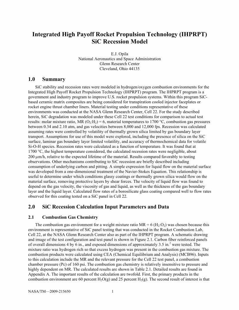
Pratt & Whitney provided gas pressures and velocities over the length of the test panel for the case of MR = 6 and Pc = 160 psi (STO07a). These data are shown in Table 2.2 in two sets of units. Recession rates were calculated at the leading edge and trailing edge of the panel at those conditions highlighted in yellow. Leading edge pressures were higher and velocities lower. Trailing edge pressures were lower and gas velocities higher as the gas expanded over the panel. These conditions are expected to bound the recession rates observed for this panel.

NASA/TM—2009-215650 3

TABLE 2.2.—COMBUSTION GAS PRESSURES AND VELOCITIES AS A FUNCTION OF POSITION ALONG TEST PANEL IN DIRECTION OF FLOW X Pinf Vinf X Pinf Vinf

(in.) (psia) (ft/sec) (cm) (atm) (cm/s)

0.00 30.82 8407.1 0 2.09681 256247.2 0.07 30.82 8407.1 0.167896 2.09681 256247.2 0.16 29.59 8503.2 0.404908 2.012733 259176.8 0.27 28.39 8598.5 0.67382 1.931432 262082.3 0.37 27.24 8693.1 0.930837 1.85283 264964.9 0.47 26.12 8786.9 1.19812 1.776856 267825.4 0.59 25.04 8880.1 1.500489 1.703439 270664.8 0.70 24.00 8972.6 1.790666 1.632511 273483.8 0.82 22.99 9064.4 2.092651 1.564006 276283.2 0.96 22.02 9155.6 2.433293 1.49786 279063.7 1.09 21.08 9246.3 2.76162 1.434011 281825.8 1.22 20.17 9336.3 3.103593 1.372398 284570.1 1.37 19.30 9425.8 3.488247 1.312962 287297.3 1.52 18.46 9514.7 3.860669 1.255645 290007.7 1.67 17.65 9603.1 4.248932 1.200389 292701.8 1.84 16.86 9690.9 4.684429 1.14714 295380.1 2.01 16.11 9778.3 5.108034 1.095843 298042.9 2.19 15.38 9865.2 5.550101 1.046444 300690.7 2.38 14.68 9951.6 6.044586 0.998889 303323.7 2.57 14.01 10037.5 6.527837 0.953128 305942.3 2.77 13.36 10122.9 7.032684 0.90911 308546.8 2.99 12.74 10207.9 7.59588 0.866784 311137.5 3.21 12.14 10292.5 8.1489 0.826101 313714.6 3.44 11.57 10376.6 8.727275 0.787013 316278.4 3.80 10.11 10604.0 9.654918 0.688071 323209.8 4.22 8.82 10828.3 10.73056 0.599726 330048 4.68 7.66 11049.8 11.88618 0.521089 336796.6 5.19 6.63 11268.3 13.18049 0.451318 343458.6 5.78 5.73 11484.1 14.69276 0.389615 350036.7 6.00 5.42 11560.1 15.24 0.368751 352351.8 6.43 4.93 11697.3 16.34254 0.335231 356533.1

2.4 Thermochemical Data for Volatile Si-O-H Species

Volatility of SiO2 (silica) or SiC results from the formation of stable gas species such as SiO(g), Si(OH)4(g), SiO(OH)(g), and SiO(OH)2(g) which consumes the starting material. The stability of these vapor species in the combustion environment was calculated using a free energy minimization technique. This calculation involves inputting the reactants SiO2 or SiC and the combustion gas reactants: H2O, H2, OH, H, O, and O2 into free energy minimization software, FACTSAGE (BAL02). The free energy minimization takes this reactant assemblage, and using thermochemical data for these species, calculates the equilibrium product assemblage with the lowest free energy, i.e., the most stable product combination. In order to calculate the partial pressures of these volatile Si-O-H(g) products, thermochemical data for all these species must be available in the software database. Data for the Si-O-H(g) species are not generally included in thermochemical databases, so data from various sources was input into the FACTSAGE database. Data for the following vapor species was input from the cited references: SiO(g) already present in FACT53 database (BAL02), Si(OH)4(g) (JAC05), SiO(OH)2(g) (JAC05), and SiO(OH)(g) (ALL95). These data are discussed in more detail in Section 4.3. The preferred recession rates reported here make use of the Allendorf (ALL95) data for SiO(OH)(g). Alternative calculations using the Krikorian data for SiO(OH)(g) (KRI70) are presented and discussed in Section 4.3.1.4.

NASA/TM—2009-215650 4

3.0 Recession Calculations

3.1 Calculation of Volatile Species Partial Pressures

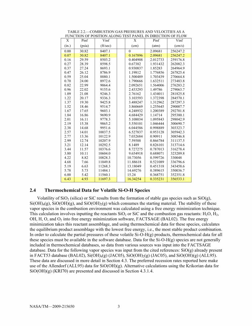
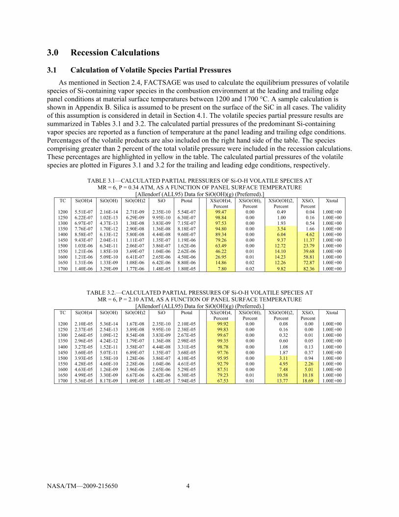
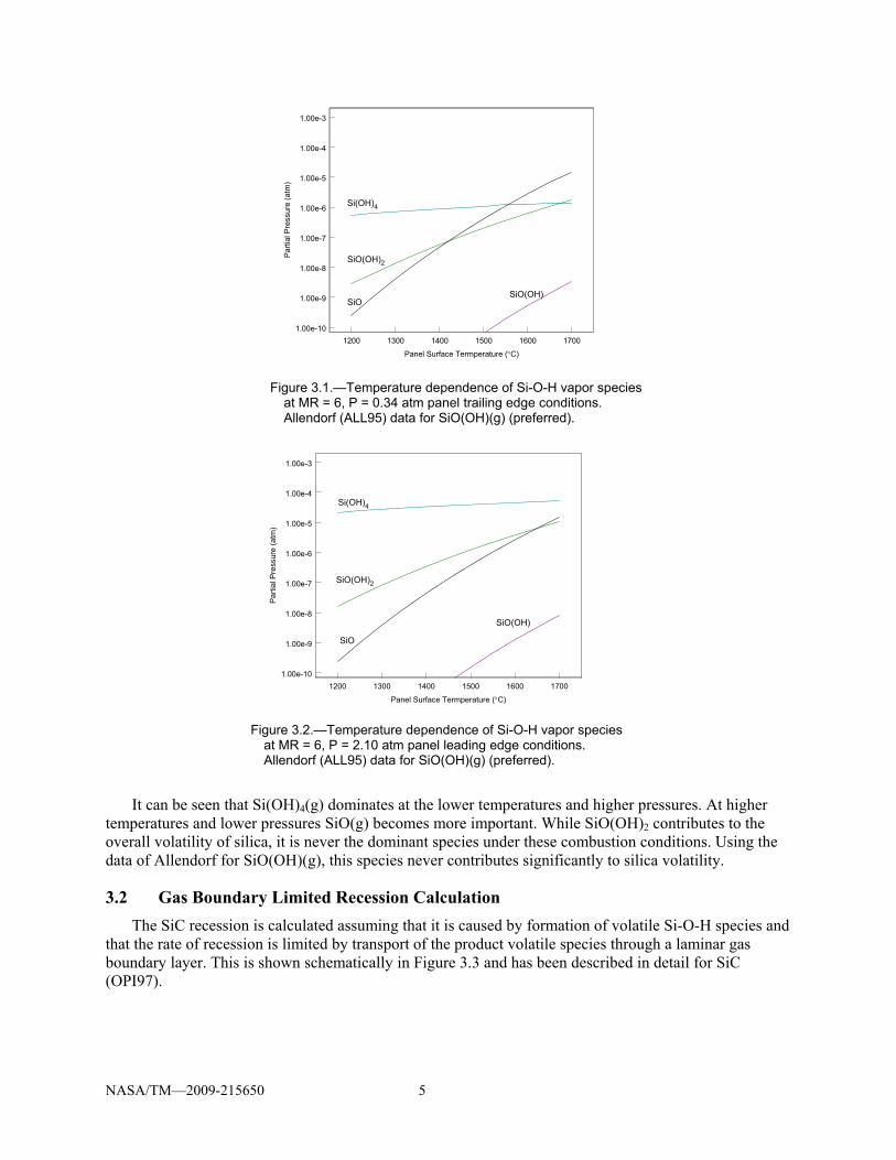
As mentioned in Section 2.4, FACTSAGE was used to calculate the equilibrium pressures of volatile species of Si-containing vapor species in the combustion environment at the leading and trailing edge panel conditions at material surface temperatures between 1200 and 1700 °C. A sample calculation is shown in Appendix B. Silica is assumed to be present on the surface of the SiC in all cases. The validity of this assumption is considered in detail in Section 4.1. The volatile species partial pressure results are summarized in Tables 3.1 and 3.2. The calculated partial pressures of the predominant Si-containing vapor species are reported as a function of temperature at the panel leading and trailing edge conditions. Percentages of the volatile products are also included on the right hand side of the table. The species comprising greater than 2 percent of the total volatile pressure were included in the recession calculations. These percentages are highlighted in yellow in the table. The calculated partial pressures of the volatile species are plotted in Figures 3.1 and 3.2 for the trailing and leading edge conditions, respectively.

TABLE 3.1—CALCULATED PARTIAL PRESSURES OF Si-O-H VOLATILE SPECIES AT MR = 6, P = 0.34 ATM, AS A FUNCTION OF PANEL SURFACE TEMPERATURE

[Allendorf (ALL95) Data for SiO(OH)(g) (Preferred).] TC Si(OH)4 SiO(OH) SiO(OH)2 SiO Ptotal XSi(OH)4,

Percent XSiO(OH),

Percent XSiO(OH)2,

Percent XSiO, Percent

Xtotal

1200 5.51E-07 2.16E-14 2.71E-09 2.35E-10 5.54E-07 99.47 0.00 0.49 0.04 1.00E+00 1250 6.22E-07 1.02E-13 6.29E-09 9.95E-10 6.30E-07 98.84 0.00 1.00 0.16 1.00E+00 1300 6.97E-07 4.37E-13 1.38E-08 3.83E-09 7.15E-07 97.53 0.00 1.93 0.54 1.00E+00 1350 7.76E-07 1.70E-12 2.90E-08 1.36E-08 8.18E-07 94.80 0.00 3.54 1.66 1.00E+00 1400 8.58E-07 6.13E-12 5.80E-08 4.44E-08 9.60E-07 89.34 0.00 6.04 4.62 1.00E+00 1450 9.43E-07 2.04E-11 1.11E-07 1.35E-07 1.19E-06 79.26 0.00 9.37 11.37 1.00E+00 1500 1.03E-06 6.34E-11 2.06E-07 3.86E-07 1.62E-06 63.49 0.00 12.72 23.79 1.00E+00 1550 1.21E-06 1.85E-10 3.69E-07 1.04E-06 2.62E-06 46.22 0.01 14.10 39.68 1.00E+00 1600 1.21E-06 5.09E-10 6.41E-07 2.65E-06 4.50E-06 26.95 0.01 14.23 58.81 1.00E+00 1650 1.31E-06 1.33E-09 1.08E-06 6.42E-06 8.80E-06 14.86 0.02 12.26 72.87 1.00E+00 1700 1.40E-06 3.29E-09 1.77E-06 1.48E-05 1.80E-05 7.80 0.02 9.82 82.36 1.00E+00

TABLE 3.2.—CALCULATED PARTIAL PRESSURES OF Si-O-H VOLATILE SPECIES AT MR = 6, P = 2.10 ATM, AS A FUNCTION OF PANEL SURFACE TEMPERATURE

[Allendorf (ALL95) Data for SiO(OH)(g) (Preferred).] TC Si(OH)4 SiO(OH) SiO(OH)2 SiO Ptotal XSi(OH)4,

Percent XSiO(OH),

Percent XSiO(OH)2,

Percent XSiO, Percent

Xtotal

1200 2.10E-05 5.36E-14 1.67E-08 2.35E-10 2.10E-05 99.92 0.00 0.08 0.00 1.00E+00 1250 2.37E-05 2.54E-13 3.89E-08 9.95E-10 2.38E-05 99.83 0.00 0.16 0.00 1.00E+00 1300 2.66E-05 1.09E-12 8.54E-08 3.83E-09 2.67E-05 99.67 0.00 0.32 0.01 1.00E+00 1350 2.96E-05 4.24E-12 1.79E-07 1.36E-08 2.98E-05 99.35 0.00 0.60 0.05 1.00E+00 1400 3.27E-05 1.52E-11 3.58E-07 4.44E-08 3.31E-05 98.78 0.00 1.08 0.13 1.00E+00 1450 3.60E-05 5.07E-11 6.89E-07 1.35E-07 3.68E-05 97.76 0.00 1.87 0.37 1.00E+00 1500 3.93E-05 1.58E-10 1.28E-06 3.86E-07 4.10E-05 95.95 0.00 3.11 0.94 1.00E+00 1550 4.28E-05 4.60E-10 2.28E-06 1.04E-06 4.61E-05 92.79 0.00 4.95 2.26 1.00E+00 1600 4.63E-05 1.26E-09 3.96E-06 2.65E-06 5.29E-05 87.51 0.00 7.48 5.01 1.00E+00 1650 4.99E-05 3.30E-09 6.67E-06 6.42E-06 6.30E-05 79.23 0.01 10.58 10.18 1.00E+00 1700 5.36E-05 8.17E-09 1.09E-05 1.48E-05 7.94E-05 67.53 0.01 13.77 18.69 1.00E+00

NASA/TM—2009-215650 5

1200 1300 1400 1500 1600 1700

Panel Surface Termperature (C)

1.00e-10

1.00e-9

1.00e-8

1.00e-7

1.00e-6

1.00e-5

1.00e-4

1.00e-3

Par

tial P

ress

ure

(a

tm)

Si(OH)4

SiO(OH)2

SiO(OH)SiO

Figure 3.1.—Temperature dependence of Si-O-H vapor species at MR = 6, P = 0.34 atm panel trailing edge conditions. Allendorf (ALL95) data for SiO(OH)(g) (preferred).

1200 1300 1400 1500 1600 1700

Panel Surface Termperature (C)

1.00e-10

1.00e-9

1.00e-8

1.00e-7

1.00e-6

1.00e-5

1.00e-4

1.00e-3

Pa

rtia

l Pre

ssur

e (

atm

)

Si(OH)4

SiO(OH)2

SiO(OH)

SiO

Figure 3.2.—Temperature dependence of Si-O-H vapor species at MR = 6, P = 2.10 atm panel leading edge conditions. Allendorf (ALL95) data for SiO(OH)(g) (preferred).

It can be seen that Si(OH)4(g) dominates at the lower temperatures and higher pressures. At higher

temperatures and lower pressures SiO(g) becomes more important. While SiO(OH)2 contributes to the overall volatility of silica, it is never the dominant species under these combustion conditions. Using the data of Allendorf for SiO(OH)(g), this species never contributes significantly to silica volatility.

3.2 Gas Boundary Limited Recession Calculation

The SiC recession is calculated assuming that it is caused by formation of volatile Si-O-H species and that the rate of recession is limited by transport of the product volatile species through a laminar gas boundary layer. This is shown schematically in Figure 3.3 and has been described in detail for SiC (OPI97).

NASA/TM—2009-215650 6

Figure 3.3—Schematic illustration of SiC volatility limited by transport of Si-O-H(g) species through a

laminar gas boundary layer for a flat plate geometry.

Assuming a flat plate geometry, the flux of volatile species, J, is given by (GEI80, GAS92):

LRT

DPM664.0

3/12/1

D

vLJ (1)

The term in the first parentheses is the dimensionless Reynolds number, while the term in the second

set of parentheses is the dimensionless Schmidt number. The symbols are defined in Table 3.3. The recession depends on gas pressures, temperature, and velocity.

TABLE 3.3.—PARAMETERS USED IN EQUATION (1)

Symbol Definition Units Comments ’ Density of gas boundary layer g/cm3 Calculated from ideal gas law v Gas velocity cm/sec Combustion gas variable L Characteristic length cm Length of panel Gas viscosity of boundary layer g/(cm sec) Obtained from tabulated values (SVE62) D Interdiffusion coefficient of volatile

species in laminar boundary layer cm2/sec Calculated from Chapman Enskog

Equation, see (GEI80) P Partial pressure of volatile species atm Predicted from thermodynamic data M Molecular weight of volatile species g/mol R Gas constant (cm3 atm) /K mol T Absolute temperature K Material surface temperature variable

A sample recession calculation is shown in Appendix C. The assumptions made in the recession

calculation Equation (1) are discussed in Appendix D. Required input to the recession calculation are the following: combustion gas pressure, material surface temperature, free stream combustion gas velocity, panel length, combustion gas viscosity (SVE62), force constants (SVE62) and collision integral (HIR54) for the volatile species and the boundary layer gas species (discussed in Appendix D), and the calculated equilibrium partial pressure of volatile Si-O-H species.

The recession attributed to the formation of each species as well as the overall recession rate in 1834 sec are reported in Table 3.4. This exposure time was chosen for comparison to GE Panel 1528-01-001-001 which actually endured nine exposures for a total plume exposure of 1834 sec. This panel is a standard matrix C/SiC panel with no oxidation protection coatings. The NASA GRC run numbers were 309 through 318. In the areas where the IR camera reported temperatures below 1723 °C, there was no measurable recession. The detectability limit of recession was estimated to be 1 mil (25 m). The calculated recession rates show that about 4 mils (0.1 mm) recession is expected at the leading edge and approximately an order of magnitude less recession is expected at the trailing edge of the panel. The very low calculated recession values are consistent with the lack of observable recession temperatures below the melting point of SiO2.

L

H2O gas flow, gas boundary layer

Si-O-H(g)

SiO2 =0

free stream gas

NASA/TM—2009-215650 7

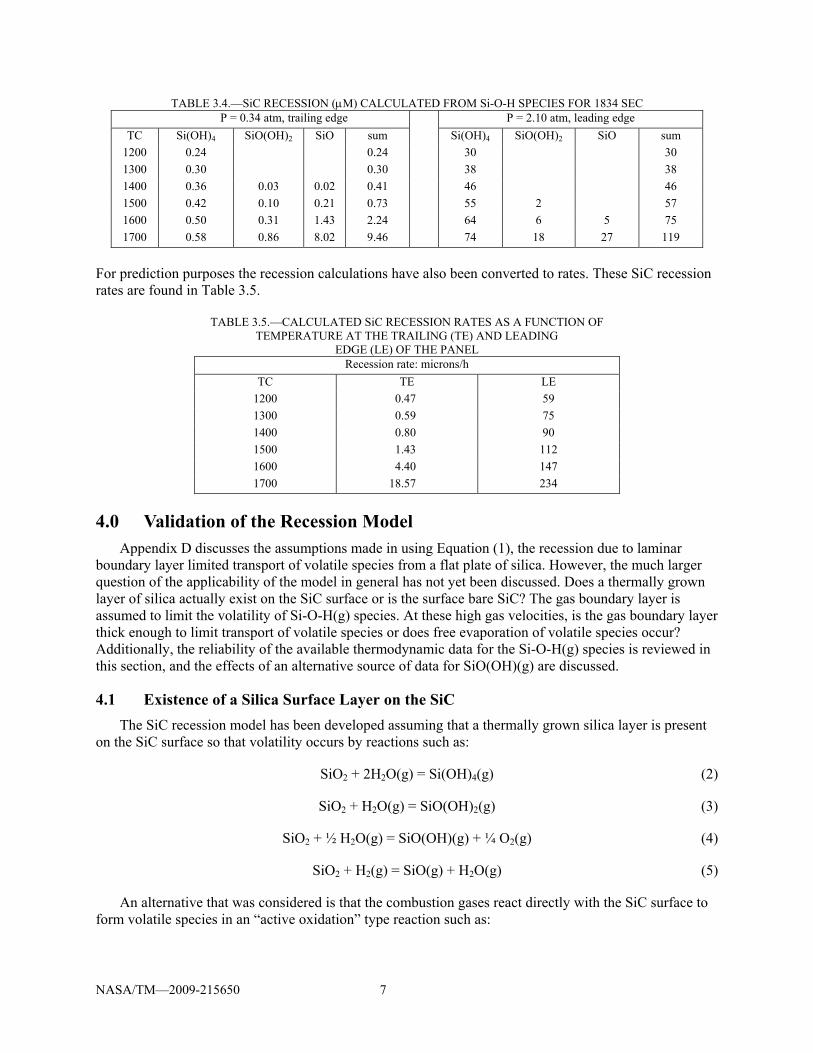
TABLE 3.4.—SiC RECESSION (M) CALCULATED FROM Si-O-H SPECIES FOR 1834 SEC P = 0.34 atm, trailing edge P = 2.10 atm, leading edge

TC Si(OH)4 SiO(OH)2 SiO sum Si(OH)4 SiO(OH)2 SiO sum

1200 0.24 0.24 30 30

1300 0.30 0.30 38 38

1400 0.36 0.03 0.02 0.41 46 46

1500 0.42 0.10 0.21 0.73 55 2 57

1600 0.50 0.31 1.43 2.24 64 6 5 75

1700 0.58 0.86 8.02 9.46 74 18 27 119

For prediction purposes the recession calculations have also been converted to rates. These SiC recession rates are found in Table 3.5.

TABLE 3.5.—CALCULATED SiC RECESSION RATES AS A FUNCTION OF TEMPERATURE AT THE TRAILING (TE) AND LEADING

EDGE (LE) OF THE PANEL Recession rate: microns/h

TC TE LE

1200 0.47 59

1300 0.59 75

1400 0.80 90

1500 1.43 112

1600 4.40 147

1700 18.57 234

4.0 Validation of the Recession Model Appendix D discusses the assumptions made in using Equation (1), the recession due to laminar

boundary layer limited transport of volatile species from a flat plate of silica. However, the much larger question of the applicability of the model in general has not yet been discussed. Does a thermally grown layer of silica actually exist on the SiC surface or is the surface bare SiC? The gas boundary layer is assumed to limit the volatility of Si-O-H(g) species. At these high gas velocities, is the gas boundary layer thick enough to limit transport of volatile species or does free evaporation of volatile species occur? Additionally, the reliability of the available thermodynamic data for the Si-O-H(g) species is reviewed in this section, and the effects of an alternative source of data for SiO(OH)(g) are discussed.

4.1 Existence of a Silica Surface Layer on the SiC

The SiC recession model has been developed assuming that a thermally grown silica layer is present on the SiC surface so that volatility occurs by reactions such as:

SiO2 + 2H2O(g) = Si(OH)4(g) (2)

SiO2 + H2O(g) = SiO(OH)2(g) (3)

SiO2 + ½ H2O(g) = SiO(OH)(g) + ¼ O2(g) (4)

SiO2 + H2(g) = SiO(g) + H2O(g) (5)

An alternative that was considered is that the combustion gases react directly with the SiC surface to

form volatile species in an “active oxidation” type reaction such as:

NASA/TM—2009-215650 8

SiC + 2H2O = SiO(g) + CO(g) + 2H2(g) (6) SiC + 4H2O = SiO(OH)2(g) + CO(g) + 3H2(g) (7) SiC + 5H2O = Si(OH)4(g) + CO(g) + 3H2(g) (8)

The existence of SiO2 on the SiC surface for MR = 6 conditions is shown to exist by a number of methods which are discussed in more detail in the following four subsections. First, FACTSAGE calculations to determine the equilibrium products were conducted for SiC plus the combustion gas reactants showing the stability of SiO2 on SiC when the calculations made physical sense. Second, the oxide thickness was estimated based on the oxidation rate of SiC and the volatility rate of SiO2. Third, these results were compared to EDS results obtained at Teledyne (CAL07). Finally, the combustion conditions were compared to the literature where active oxidation was observed in H2/H2O mixtures (KIM87).

4.1.1 FACTSAGE Calculations Indicate SiO2 is Present on the SiC Surface

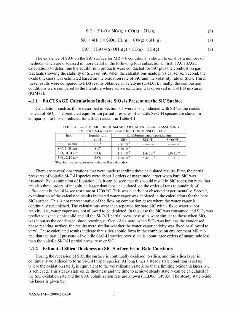
Calculations such as those described in Section 3.1 were also conducted with SiC as the reactant instead of SiO2. The predicted equilibrium partial pressures of volatile Si-O-H species are shown in comparison to those predicted for a SiO2 reactant in Table 4.1.

TABLE 4.1.—COMPARISON OF Si-O-H PARTIAL PRESSURES ASSUMING SiC VERSUS SiO2 IS THE REACTING CONDENSED PHASE

Input Equilibrium solid

Equilibrium vapor species, atm SiO Si(OH)4 SiO(OH)2

SiC, 0.34 atm SiCa 2.810–2 --------- --------- SiC, 2.10 atm SiCa 1.810–1 --------- --------- SiO2, 0.34 atm SiO2 1.510–5 1.410–6 1.810–6 SiO2, 2.10 atm SiO2 1.510–5 5.410–5 1.110–5

aReactant water vapor is depleted in this calculation

There are several observations that were made regarding these calculated results. First, the partial pressures of volatile Si-O-H species were about 3 orders of magnitude larger when bare SiC was assumed. By examination of Equation (1), it can be seen that this would result in SiC recession rates that are also three orders of magnitude larger than those calculated, on the order of tens to hundreds of millimeters in the 1834 sec test time at 1700 °C. This was clearly not observed experimentally. Second, examination of the calculated results indicated water vapor was depleted in the calculations for the bare SiC surface. This is not representative of the flowing combustion gases where the water vapor is continually replenished. The calculations were then repeated for bare SiC with a fixed water vapor activity, i.e., water vapor was not allowed to be depleted. In this case the SiC was consumed and SiO2 was predicted as the stable solid and all the Si-O-H partial pressure results were similar to those when SiO2 was input as the condensed phase reacting surface. (As a note, when SiO2 was input as the condensed phase reacting surface, the results were similar whether the water vapor activity was fixed or allowed to vary). These calculated results indicate that silica should form in the combustion environment MR = 6 and that the partial pressure of volatile Si-O-H species over silica is about three orders of magnitude less than the volatile Si-O-H partial pressure over SiC.

4.1.2 Estimated Silica Thickness on SiC Surface From Rate Constants

During the recession of SiC, the surface is continually oxidized to silica, and this silica layer is continually volatilized to form Si-O-H vapor species. At long times a steady state condition is set up where the oxidation rate kp is equivalent to the volatilization rate kl so that a limiting oxide thickness, xL, is achieved. This steady state oxide thickness and the time to achieve steady state tL can be calculated if the SiC oxidation rate and the SiO2 volatilization rate are known (TED66, OPI03). The steady state oxide thickness is given by:

NASA/TM—2009-215650 9

l

pL k

kx

2 (9)

and the time to reach this limiting oxide thickness is given by, tL:

2)(2 l

pL

k

kt (10)

These quantities have been estimated at 1700 °C based on parabolic rate constants that were extrapolated from lower temperatures and volatility rates that were calculated at 1700 °C. Details of this calculation and the assumptions made can be found in Appendix E. The results are summarized in Table 4.2.

TABLE 4.2.—ESTIMATED OXIDE THICKNESS ON SiC PANEL UNDER MR = 6 COMBUSTION CONDITIONS

Steady state oxide thickness, nm

Time to reach steady state, sec

Leading edge 19 0.1 Trailing edge 38 3

In summary, a silica layer thickness on the order of tens of nm is predicted to be present on the surface of SiC. This layer should protect the SiC from active oxidation type reactions.

4.1.3 Estimated Silica Thickness on SiC From EDS Measurements

Using the available EDS resources and without destructively analyzing the sample, Calabrese (CAL07) and coworkers were able to estimate the silica thickness on the surface of panel 1528-01-001-002 GE standard SiC seal coat tested for 16 min in Cell 22. By varying the electron accelerating voltage and calibrating the EDS oxygen signal to sampling volume for a silica film of known thickness, the silica film thickness near the leading edge of the SiC panel was estimated to be 10 nm. Portions of the panel downstream and in cooler areas had thicker estimated silica film thicknesses of 15 to 63 nm. The analyses were conducted on relatively large areas to prevent interpretation issues relative to the shape of the sampling volume. The actual pitted surface morphology suggests that there are inhomogeneities at a very small scale, but the analysis could not probe at that level of detail. The pitting will be discussed in more detail in Section 5.0. Nevertheless, the oxide thickness estimated from the experimental EDS results are in good agreement with the oxide thickness estimated from the rate constants in Section 4.1.2. The oxide thickness on the SiC panels in the flow stream is therefore likely on the order of tens of nanometers.

4.1.4 Comparison of Cell 22 Conditions to Active Oxidation Conditions Reported in the Literature

Active oxidation of SiC is known to occur in H2/H2O environments by reaction 6 as shown by Kim and Readey (KIM87). It has been demonstrated that the active to passive transition depends on the partial pressure of the oxidant (H2O in this case), independent of the H2O/H2 ratio (OPI95). These results were extrapolated to 1700 C, for the purposes of the assumed temperature of the Cell 22 panel result modeling as shown in Figure 4.1. This plot is used to find the pressure at which the transition between two gas phase processes occurs. At lower oxidant pressures than the transition pressure SiO(g) is formed directly from SiC. At higher oxidant pressures than the transition pressure, SiO2 will form. However, this transition pressure is not a well-defined cut-off for weight loss by volatility reactions. It has been experimentally observed (KIM87) that weight loss will continue at higher pressures because of formation of a discontinuous silica scale as well as the reduction of silica to form SiO(g) by:

SiO2 = SiO(g) + ½ O2(g) (11)

This is shown by Kim and Readey’s results in Figure 4.2.

NASA/TM—2009-215650 10

5.0 5.2 5.4 5.6 5.8 6.0

10,000/T(K)

10-5

10-4

10-3

10-2

norm

aliz

ed tr

ansi

tion

pres

sure

(at

m)

[KIM87], H2O[NAR93], CO2[NAR91], O21700C

Figure 4.1.—Active to passive transition for SiC forming SiO(g) as a function of oxidant partial pressure extrapolated to 1700 °C (OPI95).

10-5 10-4 10-3 10-2

PH2O (atm)

10-8

10-7

10-6

10-5

flux

(g/c

m2 s

ec)

discontinuous silica scale or

oxidation-reduction

active oxidation

1400C

1427C

1450C

1475C

1500C

1527C

Figure 4.2.—Active to passive transition pressures for SiC. From Kim and Readey

(KIM87).

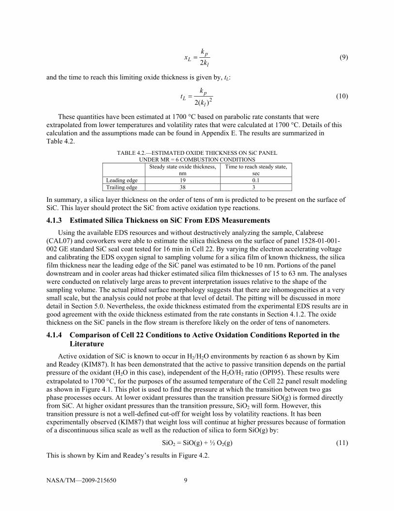
The solid symbols show the measured active to passive transition pressures. To the left of the maxima (low oxidant pressures), the weight loss rate increases with oxidant pressure as more SiO(g) is formed. To the right of the maxima, the weight loss rate decreases with oxidant pressure because more SiO2(s) is formed, partially covering the surface. The rate of SiO(g) formation may also decrease as the reduction of SiO2 becomes more unfavorable at higher oxidant pressures. At even higher oxidant pressures than shown on this plot, weight gain occurs as protective silica formation occurs. Extrapolating the maxima to 1700 C and the active to passive transition pressure at 1700 C, it can be seen where the Cell 22 conditions fall on this plot, as shown in Figure 4.3. From this plot, it is evident that the cell 22 conditions

NASA/TM—2009-215650 11

10-5 10-4 10-3 10-2 10-1 100

PH2O, atm

10-7

10-6

10-5

10-4

10-3

flux

(g/c

m2 s

ec)

active oxidation discontinuous silica scale or

oxidation-reduction

MR=6.0

1400C1427C1450C1475C1500C1527C

1700C

Figure 4.3.—Active to passive transition data of Kim and Readey extrapolated to conditions of interest for Cell 22 tests.

MR = 6 are really quite oxidizing (60 percent H2O/25 percent H2) and are well within the oxidant pressure range where a film of SiO2 is expected on the surface of SiC. Weight loss may still be possible as the SiO2 film may be discontinuous or be lost by reaction of SiO2 to form volatile species.

The data plotted in Figure 4.2 were determined at very low gas velocities, on the order of 1 cm/sec. From Wagner’s theory (WAG58), the active to passive transition oxidant pressure should be relatively independent of gas velocity. The flux of species X, H2O(g) inward to the SiC surface or SiO(g) outward from the surface, is given by:

RT

PDJ

X

XXX (12)

The transition pressure is obtained by equating the flux of oxidant inward to the SiO(g) flux outward. So that:

)SiO()OH(

)iOS(

)SiO(

)OH()OH( eq

2

22

transition PD

DP

(13)

The velocity dependence of each flux is contained within the boundary layer thickness term, . In

Figures 4.2 and 4.3, each temperature curve would be expected to shift up as the velocity increases. The SiO(g) flux will increase as the boundary layer thickness is decreased. However, it is expected that the gas boundary layer thickness would be similar for the oxidant and the SiO(g) so that the transition pressure should be independent of gas velocity. According to Wagner, each temperature curve in Figures 4.2 and 4.3 is not expected to move to the right or left as the velocity is increased.

In actual experimental observations, however, a small shift in the active to passive transition with velocity changes has been observed (NAR91) so that a velocity increase expands the passive regime to

NASA/TM—2009-215650 12

lower oxidant pressures. This velocity dependence is not well understood but was explained as a change the boundary layer ratio [oxidant)/SiO)] or a deviation from the equilibrium pressure, P(SiO), at the SiC surface (NAR91). Since this effect actually expands the passive regime, the Cell 22 conditions would remain well inside the passive regime even if velocity effects do occur.

In summary, the analyses in Sections 4.1.1 to 4.1.4 are in consistent agreement that a silica film should be present on the SiC surface in the Cell 22 conditions of interest. This aspect of the recession model is therefore believed to be accurate.

4.2 Gas Boundary Layer Limited Volatilization

The gas flow in Cell 22 (and other rocket engine environments) occurs at very high velocities, 8,000 to 12,000 fps. At these high gas velocities the gas boundary layer becomes very thin. The recession model assumes that volatility is limited by transport of volatile species through the gas boundary layer. It is important to understand how thin the gas boundary layer is under the Cell 22 test conditions and at what point volatility is better modeled by the free evaporation rate given by the Langmuir Equation. An expression for the gas boundary layer thickness is given by (GRA71):

3/12/1Re

5.1

Sc

L (14)

where

LRe (15)

D

Sc

(16)

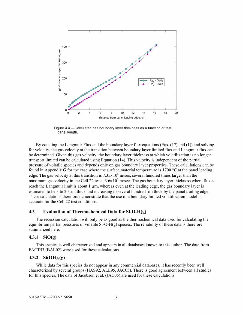
First, the gas boundary layer thickness, , along length of panel was calculated using the local Reynolds number, Rex, for PC160MR60 provided by Jeff Stout (STO07b). The length averaged ReL calculated using Equation (15) was also used to calculate the gas boundary layer thickness. The Reynolds numbers are reported in Appendix F. Both results are shown in Figure 4.4. The calculated gas boundary layer thickness varies from a few microns at the leading edge of the panel to a few hundred microns at the trailing edge of the panel. Again this is based on laminar flow. The exponent for the Reynolds number in the gas boundary layer calculation increases to 0.7 or 0.8 for turbulent flow (GAS92) which would decrease the boundary layer thickness. The Stout Rex are just in the turbulent flow regime for all x, assuming the laminar—turbulent flow transition occurs for Re = 3105. The ReL calculated from Equation (15) transition from laminar to turbulent at about 5.5 cm (2.2 in.) from the leading edge of the panel. However, the assumption of laminar flow has little effect on the overall values of the gas boundary layer thickness.

For vanishingly thin boundary layers and high gas velocities the Hertz-Langmuir Equation can be used to calculate the flux of volatiles from a surface, JL. This equation is used to calculate the maximum evaporation reaction rate from thermodynamic data (SEA70, BAR67).

2/1SiOH

SiOH 2

RT

MPJ L

(17)

NASA/TM—2009-215650 13

0 2 4 6 8 10 12 14 16 18 20

distance from panel leading edge, cm

0

100

200

300

400

gas

boun

dary

laye

r th

ickn

ess,

m

ReL - OpilaRex - Stout

Figure 4.4.—Calculated gas boundary layer thickness as a function of test panel length.

By equating the Langmuir Flux and the boundary layer flux equations (Eqs. (17) and (1)) and solving

for velocity, the gas velocity at the transition between boundary layer limited flux and Langmuir flux can be determined. Given this gas velocity, the boundary layer thickness at which volatilization is no longer transport limited can be calculated using Equation (14). This velocity is independent of the partial pressure of volatile species and depends only on gas boundary layer properties. These calculations can be found in Appendix G for the case where the surface material temperature is 1700 °C at the panel leading edge. The gas velocity at this transition is 7.35105 m/sec, several hundred times larger than the maximum gas velocity in the Cell 22 tests, 3.6103 m/sec. The gas boundary layer thickness where fluxes reach the Langmuir limit is about 1 m, whereas even at the leading edge, the gas boundary layer is estimated to be 3 to 20 m thick and increasing to several hundred m thick by the panel trailing edge. These calculations therefore demonstrate that the use of a boundary limited volatilization model is accurate for the Cell 22 test conditions.

4.3 Evaluation of Thermochemical Data for Si-O-H(g)

The recession calculation will only be as good as the thermochemical data used for calculating the equilibrium partial pressures of volatile Si-O-H(g) species. The reliability of these data is therefore summarized here.

4.3.1 SiO(g)

This species is well characterized and appears in all databases known to this author. The data from FACT53 (BAL02) were used for these calculations.

4.3.2 Si(OH)4(g)

While data for this species do not appear in any commercial databases, it has recently been well characterized by several groups (HAS92, ALL95, JAC05). There is good agreement between all studies for this species. The data of Jacobson et al. (JAC05) are used for these calculations.

NASA/TM—2009-215650 14

4.3.3 SiO(OH)2(g)

There are limited experimental data for this species (JAC05, HIL94, HIL98). Additional estimated data are given by Krikorian (KRI70). Preference is given to experimental data, therefore, the data of Jacobson et al (JAC05) have been used for these calculations. While these data are uncertain, there are no conditions where this species is predicted to dominate, thus the uncertainty of the stability of this vapor species is unlikely to affect the overall accuracy of the recession calculations.

4.3.4 SiO(OH)(g)

There is the most uncertainty for the thermodynamic data for this species. There is one possible identification of this species by experimental techniques (HIL94, HIL98) and three other sources of estimated (KRI70) or calculated data for this species (DAR93, ALL95). The thermochemical data for this vapor species, as well as the source of the data, are summarized in Table 4.3. The heats of formation fall into two groups, those in the range of –305 to –356 kJ/mol (DAR93, ALL95, HIL98, SAN07) as used in prior calculations and those around –500 kJ/mol (KRI70, HIL94). The two available values for S (KRI70, ALL95) are in better agreement. Since the enthalpy data are so uncertain, the recession rates previously calculated using the preferred values computed by Allendorf et al. (ALL95) are compared to the recession rates obtained using the data estimated by Krikorian (KRI70). The Allendorf data are preferred in this case, since they give better agreement with experimental observations in Cell 22. However, an upper bound of SiC recession attributed to SiO(OH)(g) formation is obtained using the estimated data of Krikorian (KRI70).

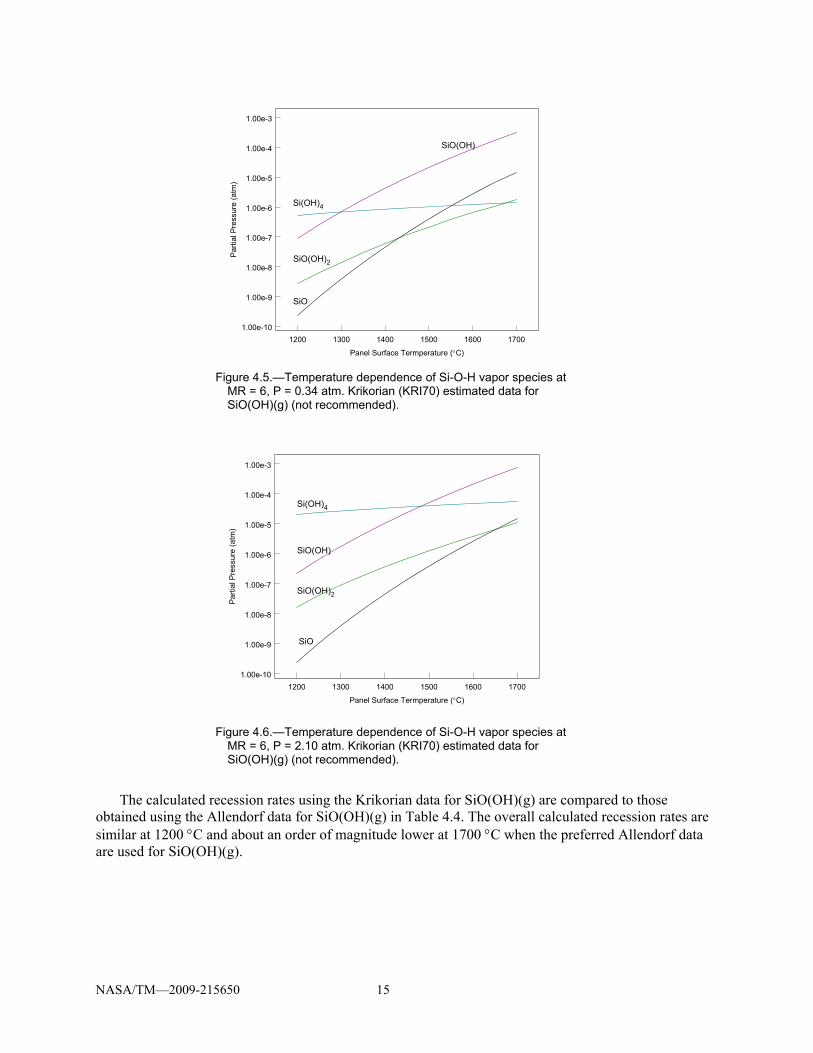
Using the thermodynamic data for SiO(OH)(g) of Krikorian, the partial pressures of all volatile Si-O-H species were calculated between the temperatures of 1200 and 1700 C for the Cell 22 conditions. The results are plotted for the Si-O-H species with the four highest partial pressures in Figures 4.5 and 4.6. Raw data can be found in Appendix G. The calculated partial pressures of SiO(OH)(g) are five to seven orders of magnitude lower using the data of Allendorf compared to the data of Krikorian. With the Allendorf data, SiO(OH)(g) does not contribute to volatility under any of the temperature and pressure conditions examined in these calculations whereas the SiO(OH)2(g) vapor species does contribute to the overall recession. Using the Krikorian data for SiO(OH)(g), Si(OH)4(g) still dominates at low temperature and high pressure conditions, but now SiO(OH)(g) exceeds the importance of SiO(g) at low pressures and high temperatures. The contributions of SiO(OH)2(g) are now negligible. While the Allendorf data for SiO(OH)(g) are preferred due to the better agreement with experimental results, this comparison shows that greater uncertainty in recession calculations is present at the high temperature, low pressure conditions.

TABLE 4.3.—THERMOCHEMICAL DATA AVAILABLE FOR SiO(OH)(g) Reference Hf(TK),

kJ/mol S,

J/mol Method of

determination Comments

Krikorian (KRI70) –4944, 0 K --- Estimation GEF available Krikoriana (KRI70) –5034, 298 K 263 Estimation Derived from GEF Darling (DAR93) –3058, 298 K --- Calculation G2 Hildenbrand (HIL94) –49417, 298 K --- Expt., mass spec Allendorf (ALL95) –3136, 298 K 271 Calculation BAC-MP4 Hildenbrand (HIL98) <–356, 298 K --- Expt., mass spec Revised from (HIL94) Sandia (SAN07) Same as (ALL95) Cp(T) available

aUsed in prior recession calculations

NASA/TM—2009-215650 15

1200 1300 1400 1500 1600 1700

Panel Surface Termperature (C)

1.00e-10

1.00e-9

1.00e-8

1.00e-7

1.00e-6

1.00e-5

1.00e-4

1.00e-3

Par

tial P

ress

ure

(atm

)

Si(OH)4

SiO(OH)2

SiO(OH)

SiO

Figure 4.5.—Temperature dependence of Si-O-H vapor species at MR = 6, P = 0.34 atm. Krikorian (KRI70) estimated data for SiO(OH)(g) (not recommended).

1200 1300 1400 1500 1600 1700

Panel Surface Termperature (C)

1.00e-10

1.00e-9

1.00e-8

1.00e-7

1.00e-6

1.00e-5

1.00e-4

1.00e-3

Pa

rtia

l Pre

ssur

e (a

tm)

Si(OH)4

SiO(OH)2

SiO(OH)

SiO

Figure 4.6.—Temperature dependence of Si-O-H vapor species at MR = 6, P = 2.10 atm. Krikorian (KRI70) estimated data for SiO(OH)(g) (not recommended).

The calculated recession rates using the Krikorian data for SiO(OH)(g) are compared to those

obtained using the Allendorf data for SiO(OH)(g) in Table 4.4. The overall calculated recession rates are similar at 1200 C and about an order of magnitude lower at 1700 C when the preferred Allendorf data are used for SiO(OH)(g).

NASA/TM—2009-215650 16

TABLE 4.4.—CALCULATED SIC RECESSION DUE TO SI-O-H VOLATILITY FOR 1834 SEC EXPOSURE AT MR = 6 AT P = 2.10 ATM (LEADING EDGE) AND P = 0.34 ATM (TRAILING EDGE) OF PANEL IN CELL 22

[Comparison of Krikorian to Allendorf data for SiO(OH)(g).] SiC recession calculated from Si-O-H species, m

with Krikorian data for SiO(OH) (NOT RECOMMENDED)

P = 0.34 atm P = 2.10 atm

TC Si(OH)4 SiO(OH) SiO Sum Si(OH)4 SiO(OH) Sum

1200 0.24 0.03 ---- 0.27 30 ---- 30

1300 0.30 0.27 ---- 0.57 38 2 40

1400 0.36 1.65 ---- 2.01 46 14 60

1500 0.42 8.35 ---- 8.77 55 68 123

1600 ---- 34 1.43 35.43 64 283 347

1700 ---- 123 8.02 131.02 74 1024 1098

with Allendorf data for SiO(OH) (PREFERRED)

P = 0.34 atm P = 2.10 atm

TC Si(OH)4 SiO(OH)2 SiO Sum Si(OH)4 SiO(OH)2 SiO Sum

1200 0.24 ---- ---- 0.24 30 ---- ---- 30

1300 0.30 ---- ---- 0.30 38 ---- ---- 38

1400 0.36 0.03 0.02 0.41 46 ---- ---- 46

1500 0.42 0.10 0.21 0.73 55 2 ---- 57

1600 0.50 0.31 1.43 2.24 64 6 5 75

1700 0.58 0.86 8.02 9.46 74 18 27 119

5.0 Other Mechanisms Contributing to SiC Degradation in Addition to Silica Volatility

Sudre and coworkers (SUD06) describe the failure of Cell 22 C/SiC test panels by a sequence of SiC cracking, pitting, grooving, oxidation of underlying carbon fibers, and eventual spallation of the SiC seal coat as shown in Figure 5.1. This mechanism results in greater recession rates than the volatility mechanism since the entire SiC coating tends to spall once the degradation occurs.

Figure 5.1.—Grooving and pitting of SiC surface after test in Cell 22. (Test panel GE 1528-01-001-002) Image courtesy of O. Sudre, Q. Yang, and D. Marshall, Teledyne Scientific (SUD06).

NASA/TM—2009-215650 17

5.1 Cracking

Presumably the cracks in the SiC arise due to the thermal expansion mismatch of the carbon fibers and the SiC matrix/seal coat. For C/C composites coated with SiC, cracks have been observed to follow the weave pattern of the fibers and to occur at regular intervals based on the stresses generated during cool down from the processing condition. (JAC07). These stress states could be modeled for the C/SiC composite leading to an understanding of the crack width and spacing.

5.2 Pitting

Similar SiC pitting has been observed for SiC exposed in molten salts, chlorine, and H2-rich environments (JAC86, MAR88, JAC90). Pitting occurs at several locations:

(1) Structural discontinuities (dislocations, high energy surfaces). (2) Areas without protective oxide such as areas where gaseous oxidation products disrupt the SiO2

scale. Since the estimated oxide layer thickness for the Cell 22 combustion conditions is only about 10 nm, it is likely this layer could be easily disrupted leading to more rapid attack. Once disrupted, the rate of attack should be much higher as predicted by the FACTSAGE calculations for bare SiC.

(3) Areas where, due to poor combustion gas mixing, the local environment is more aggressive. Such poor mixing conditions could lead to higher temperatures where local environments are closer to the stoichiometric condition. The silica scale could be molten and locally swept away by shear forces. This mechanism is discussed in Section 6.0. Alternatively, poor mixing can also result in areas with lower water partial pressures where the combustion products are more fuel rich. These local areas could be more reducing leading to locally higher degradation rates.

5.3 Grooving

The observed grooving that occurs at the crack locations in the SiC seal coat is not understood. One possibility is that local turbulence due to the rough weave morphology of the surface causes flow instabilities and enhanced attack at these locations (SUD07). An alternative explanation is that water vapor diffuses down the pre-existing cracks and oxidization of the underlying carbon fibers occurs by the reaction: C + H2O(g) = CO(g) + H2(g) (18)

The product gases CO and H2 diffuse out through the cracks and create a locally more aggressive (reducing) environment in which active oxidation occurs. Both explanations for the observed grooving are speculation at this point and this effect requires additional understanding.

5.4 Oxidation of Underlying Carbon Fibers

A model for oxidation of C/C beneath a SiC seal coat has been developed (JAC07). At high temperatures, the oxidation rate of the underlying carbon is controlled by diffusion of the oxidant through the gas boundary layer and through the coating cracks. Since the surface carbon oxidation rate is fast relative to the oxidant transport rate, oxidation at the first available surface of the underlying carbon occurs, forming oxidation cavities beneath the cracks. Once these cavities reach dimensions of half the crack spacing, the overlying SiC will spall. The parameters that affect the oxidation rate are temperature, oxidant pressure, gas velocity, and crack width. This model could be extended to C/SiC with an overlying SiC seal coat by including oxidation of the SiC matrix.

In summary, a thermomechanical model of cracking in SiC sealed C/SiC in combination with a model of carbon fiber oxidation may be applicable to explain the observed behavior of the C/SiC panels tested in Cell 22.

NASA/TM—2009-215650 18

6.0 Shear Flow of Liquid Layers at High Temperatures Recession of solid phase silica layers was discussed in Sections 2.0 through 4.0. At material surface

temperatures greater than the melting point of silica, 1723 °C (or lower temperatures in the presence of impurities), the liquid oxide film would be expected to flow due to shear forces of the flowing combustion gases on the liquid film. Similarly, for low melting borosilicate glass coatings, shear flow is expected to remove the liquid glass layer. Both shear flow of silica and glass coatings is expected to limit the protective capability of these layers by physically removing them. Therefore an understanding of the shear forces of the flowing combustion gases on the liquid films is needed.

6.1 Modeling Shear Flow of Liquids

A simple model to understand the effects of gas and liquid properties on the shear flow of a liquid film was developed with the help of David Jacqmin at GRC (JAQ07).

Assume the configuration for a gas film flowing over a liquid film on SiC as shown in Figure 6.1.

Here, the subscript g refers to gas and l refers to liquid. Start with one-dimensional Navier-Stokes equation for the liquid film:

2

2

z

v

z

p

dt

dv

(19)

Assume the velocity does not change with time and there are no pressure gradients. The first term on

each side of Equation (19) is zero, leaving:

2

2

0z

v

(20)

BC: at z = 0, vl = 0 (21)

at z = h(x,t) z

v

z

v ll

gg

(22)

The first boundary condition is the no slip condition for a fluid at a solid surface. The velocity of the liquid is zero at the SiC surface. The second BC is the same as g = l, the shear stress in the liquid is equal to the shear stress in the gas at the interface. Also at this interface, vg = vl. Here, g = f(T), T = f(x,t), Tf(z).

Figure 6.1.—Schematic illustration of liquid film used in shear flow model.

Liquid, vl

Gas, vg

x

z

z=0

z=h

z=H

SiC

NASA/TM—2009-215650 19

Assume the liquid velocity can be described by an equation of the form: vl(z) = a + bz + cz2 (23) If there is no pressure gradient in the glass then c = 0. We also know a = 0 from the first boundary condition. Taking the first derivative of the velocity equation, Eq. (23):

b

z

vl

(24)

We know from the second boundary condition that

z

vb g

l

g

(25)

and the result is that

zz

vv g

l

gl

(26)

The term

z

vg

can be approximated by the free stream gas velocity divided by the gas boundary layer

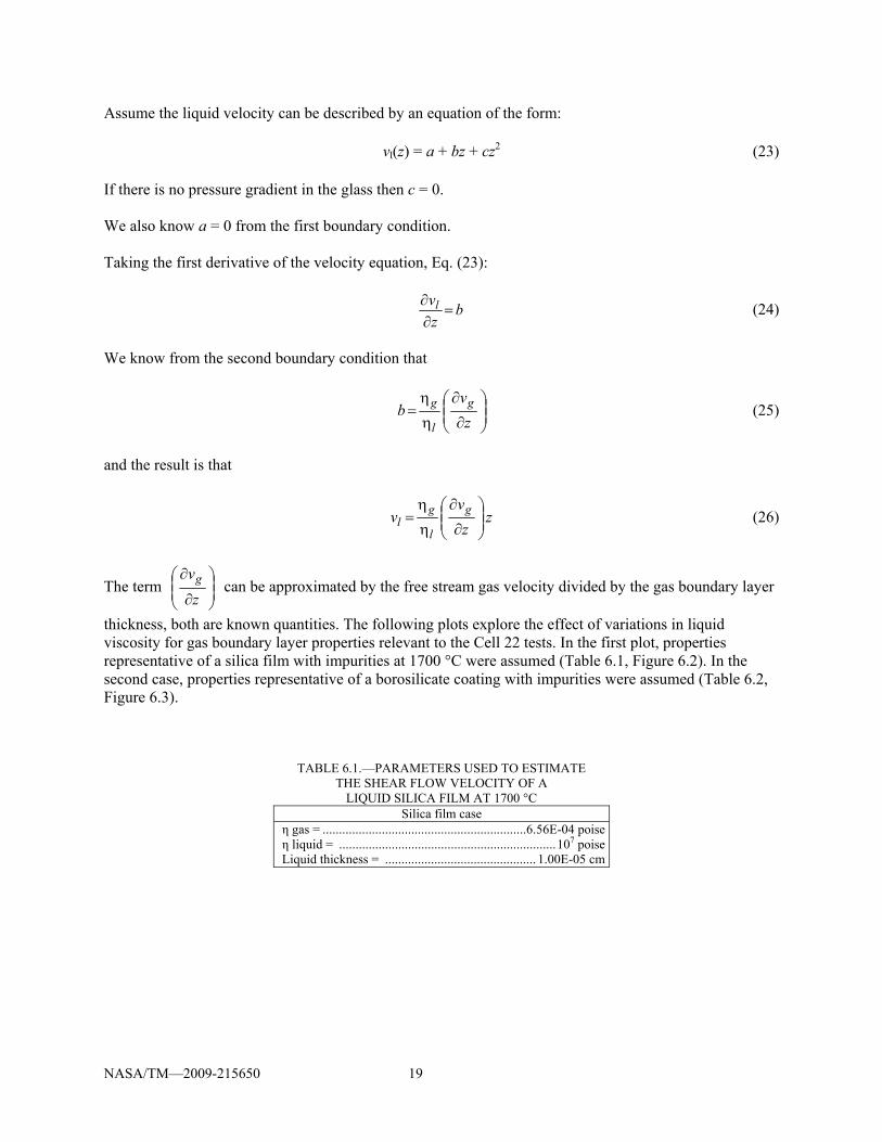
thickness, both are known quantities. The following plots explore the effect of variations in liquid viscosity for gas boundary layer properties relevant to the Cell 22 tests. In the first plot, properties representative of a silica film with impurities at 1700 °C were assumed (Table 6.1, Figure 6.2). In the second case, properties representative of a borosilicate coating with impurities were assumed (Table 6.2, Figure 6.3).

TABLE 6.1.—PARAMETERS USED TO ESTIMATE THE SHEAR FLOW VELOCITY OF A

LIQUID SILICA FILM AT 1700 °C Silica film case

η gas = .............................................................. 6.56E-04 poiseη liquid = .................................................................. 107 poiseLiquid thickness = .............................................. 1.00E-05 cm

NASA/TM—2009-215650 20

0 4 8 12 16

distance along panel, cm

0

2e-008

4e-008

6e-008

8e-008

glas

s ve

loci

ty, c

m/s

ec

Figure 6.2.—Velocity of liquid silica at 1700 °C due to shear forces from gas flow as a function of distance along the test panel.

0 4 8 12 16

distance along panel, cm

0

6

12

18

24

gla

ss v

elo

city

, cm

/se

c

borosilicate glass, calculatedsilica, calculatedborosilicate glass, measured

Figure 6.3.—Liquid glass flow velocity due to shear forces from gas flow as a function of distance along the test panel. Calculated and measured velocity of borosilicate liquid compared to silica liquid at 1700 °C.

TABLE 6.2.—PARAMETERS USED TO ESTIMATE THE

SHEAR FLOW VELOCITY OF A LIQUID BOROSILICATE FILM AT 1700 °C REPRESENTATIVE OF THE APPLIED COATING

Borosilicate coating case η gas = ......................................................................... 6.56E-04 poise η liquid = ............................................................................. 100 poise Liquid thickness = ........................................................... 2.50E-02 cm

NASA/TM—2009-215650 21

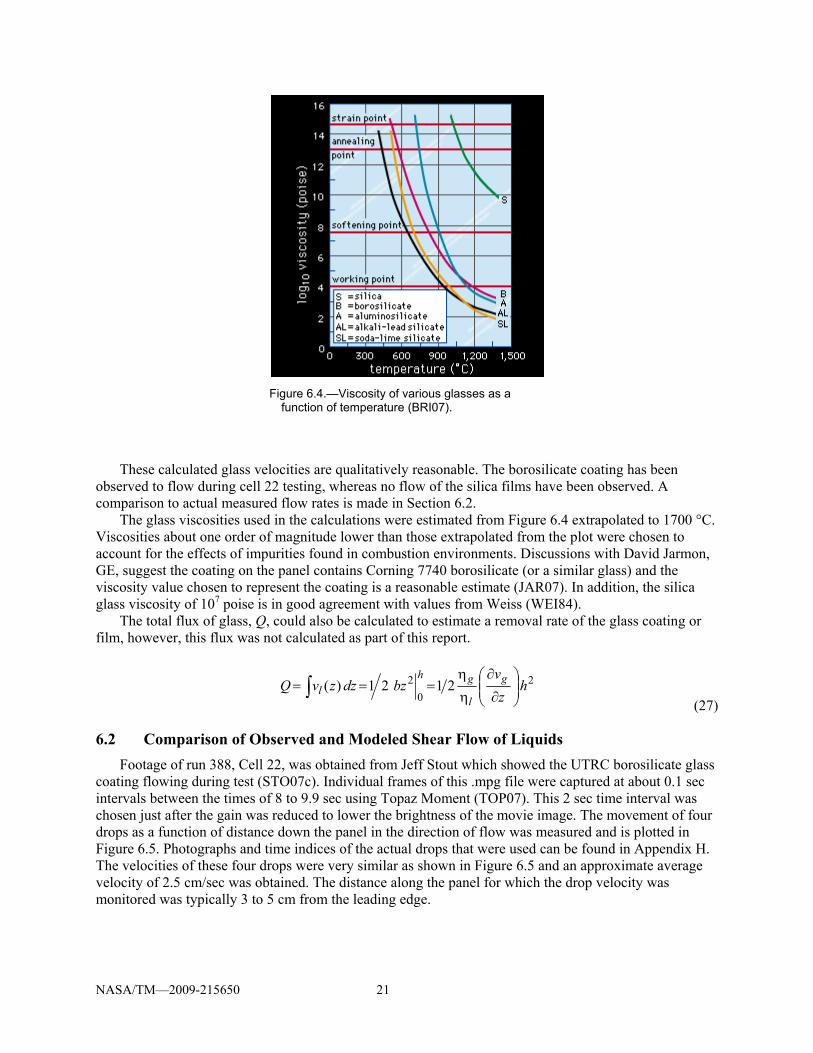
Figure 6.4.—Viscosity of various glasses as a function of temperature (BRI07).

These calculated glass velocities are qualitatively reasonable. The borosilicate coating has been

observed to flow during cell 22 testing, whereas no flow of the silica films have been observed. A comparison to actual measured flow rates is made in Section 6.2.

The glass viscosities used in the calculations were estimated from Figure 6.4 extrapolated to 1700 °C. Viscosities about one order of magnitude lower than those extrapolated from the plot were chosen to account for the effects of impurities found in combustion environments. Discussions with David Jarmon, GE, suggest the coating on the panel contains Corning 7740 borosilicate (or a similar glass) and the viscosity value chosen to represent the coating is a reasonable estimate (JAR07). In addition, the silica glass viscosity of 107 poise is in good agreement with values from Weiss (WEI84).

The total flux of glass, Q, could also be calculated to estimate a removal rate of the glass coating or film, however, this flux was not calculated as part of this report.

2

0

2 2121)( hz

vbzdzzvQ g

l

gh

l

(27)

6.2 Comparison of Observed and Modeled Shear Flow of Liquids

Footage of run 388, Cell 22, was obtained from Jeff Stout which showed the UTRC borosilicate glass coating flowing during test (STO07c). Individual frames of this .mpg file were captured at about 0.1 sec intervals between the times of 8 to 9.9 sec using Topaz Moment (TOP07). This 2 sec time interval was chosen just after the gain was reduced to lower the brightness of the movie image. The movement of four drops as a function of distance down the panel in the direction of flow was measured and is plotted in Figure 6.5. Photographs and time indices of the actual drops that were used can be found in Appendix H. The velocities of these four drops were very similar as shown in Figure 6.5 and an approximate average velocity of 2.5 cm/sec was obtained. The distance along the panel for which the drop velocity was monitored was typically 3 to 5 cm from the leading edge.

NASA/TM—2009-215650 22

0.0 0.2 0.4 0.6 0.8 1.0

time, sec

0.0

0.5

1.0

1.5

2.0

2.5

dist

ance

, cm

Figure 6.5.—Measured velocity of four glass drops on surface of panel from Cell 22 run 388.

Comparison of the measured velocity to the calculated velocity is quite good: 2.5 cm/sec measured

versus 3.5 to 4.4/sec cm calculated as shown graphically in Figure 6.3. The drop velocities do tend to slow slightly as they travel down the length of the panel, as shown in Figure 6.5, consistent with the model. The calculated liquid velocity depends on the glass and gas viscosity as well as the liquid and gas layer thickness (Eq. (26)). Since the viscosity varies strongly with temperature and all other values remain relatively constant with temperature, the liquid velocity is most strongly influenced by the viscosity of the glass for a given combustion condition and panel configuration.

NASA/TM—2009-215650 23

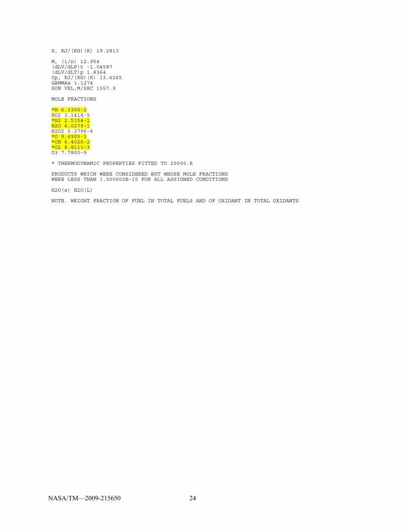
Appendix A.—CEA Calculated Combustion Products for MR = 6.0, Pc = 160 psi ******************************************************************************* NASA-LEWIS CHEMICAL EQUILIBRIUM PROGRAM CEA, SEP. 4, 1997 BY BONNIE MCBRIDE AND SANFORD GORDON REFS: NASA RP-1311, PART I, 1994 AND NASA RP-1311, PART II, 1996 ******************************************************************************* reac oxid O2 wtfrac= 1 t(k)=298.15 fuel H2 wtfrac= 1 t(k)=298.15 prob case=test hp p(psi)=160 o/f=6.0 output siunits trace=1.e-15 end OPTIONS: TP=F HP=T SP=F TV=F UV=F SV=F DETN=F SHOCK=F REFL=F INCD=F RKT=F FROZ=F EQL=F IONS=F SIUNIT=T DEBUGF=F SHKDBG=F DETDBG=F TRNSPT=F TRACE= 1.00E-15 S/R= 0.000000E+00 H/R= 0.000000E+00 U/R= 0.000000E+00 P,BAR = 11.031569 REACTANT WT.FRAC (ENERGY/R),K TEMP,K DENSITY EXPLODED FORMULA O: O2 1.000000 -.988318E-06 298.15 .0000 O 2.00000 F: H2 1.000000 -.489101E-05 298.15 .0000 H 2.00000 SPECIES BEING CONSIDERED IN THIS SYSTEM (CONDENSED PHASE MAY HAVE NAME LISTED SEVERAL TIMES) l 6/97 *H l 5/89 HO2 tpis78 *H2 l 8/89 H2O l 2/93 H2O2 l 5/97 *O tpis78 *OH tpis89 *O2 l 5/90 O3 l 8/89 H2O(s) l 8/89 H2O(L) O/F = 6.000000 EFFECTIVE FUEL EFFECTIVE OXIDANT MIXTURE ENTHALPY h(2)/R h(1)/R h0/R (KG-MOL)(K)/KG -.24262412E-05 -.30886106E-07 -.37307969E-06 KG-FORM.WT./KG bi(2) bi(1) b0i *O .00000000E+00 .62502344E-01 .53573438E-01 *H .99212255E+00 .00000000E+00 .14173179E+00 POINT ITN T O H 1 10 3354.366 -16.531 -10.113 THERMODYNAMIC EQUILIBRIUM COMBUSTION PROPERTIES AT ASSIGNED PRESSURES CASE = test REACTANT WT FRACTION ENERGY TEMP (SEE NOTE) KJ/KG-MOL K OXIDANT O2 1.0000000 .000 298.150 FUEL H2 1.0000000 .000 298.150 O/F= 6.00000 %FUEL= 14.285714 R,EQ.RATIO= 1.322780 PHI,EQ.RATIO= 1.322780 THERMODYNAMIC PROPERTIES P, BAR 11.032 T, K 3354.37 RHO, KG/CU M 5.1239-1 H, KJ/KG .00021 U, KJ/KG -2152.94 G, KJ/KG -64676.4

NASA/TM—2009-215650 24

S, KJ/(KG)(K) 19.2813 M, (1/n) 12.954 (dLV/dLP)t -1.04587 (dLV/dLT)p 1.8364 Cp, KJ/(KG)(K) 13.6265 GAMMAs 1.1274 SON VEL,M/SEC 1557.9 MOLE FRACTIONS *H 6.3300-2 HO2 3.1414-5 *H2 2.5154-1 H2O 6.0279-1 H2O2 5.3796-6 *O 9.4905-3 *OH 6.4026-2 *O2 8.8113-3 O3 7.7800-9 * THERMODYNAMIC PROPERTIES FITTED TO 20000.K PRODUCTS WHICH WERE CONSIDERED BUT WHOSE MOLE FRACTIONS WERE LESS THAN 1.000000E-15 FOR ALL ASSIGNED CONDITIONS H2O(s) H2O(L) NOTE. WEIGHT FRACTION OF FUEL IN TOTAL FUELS AND OF OXIDANT IN TOTAL OXIDANTS

NASA/TM—2009-215650 25

Appendix B.—Sample FACTSAGE Calculation for the Reaction of SiO2 and Combustion Gases at a Material Temperature of 1700 °C and the Panel

Trailing Edge Pressure, 0.34 atm

T = 1700.00 C P = 3.40000E-01 atm V = 4.37502E+02 dm3 STREAM CONSTITUENTS AMOUNT/mol H2O 6.0279E-01 H2 2.5154E-01 OH 6.4026E-02 H 6.3300E-02 O 9.4905E-03 O2 8.8113E-03 SiO2 1.0000E+00 EQUIL AMOUNT MOLE FRACTION FUGACITY PHASE: gas_ideal mol atm H2O_FACT53 6.9364E-01 7.5501E-01 2.5670E-01 H2_FACT53 2.2366E-01 2.4345E-01 8.2774E-02 H_FACT53 1.0446E-03 1.1370E-03 3.8659E-04 OH_FACT53 3.1410E-04 3.4189E-04 1.1624E-04 SiO_FACT53 4.0077E-05 4.3623E-05 1.4832E-05 SiO(OH)2_JACO 4.7792E-06 5.2021E-06 1.7687E-06 Si(OH)4_JACO 3.7934E-06 4.1290E-06 1.4039E-06 O2_FACT53 1.4152E-06 1.5404E-06 5.2375E-07 O_FACT53 1.0548E-06 1.1481E-06 3.9035E-07 SiO2H_SIO2 8.8763E-09 9.6616E-09 3.2850E-09 HOO_FACT53 1.3215E-09 1.4384E-09 4.8907E-10 HOOH_FACT53 T 8.6153E-10 9.3775E-10 3.1884E-10 Si_FACT53 3.0243E-13 3.2919E-13 1.1192E-13 SiH_FACT53 6.3502E-14 6.9121E-14 2.3501E-14 SiH4_FACT53 6.6085E-17 7.1932E-17 2.4457E-17 O3_FACT53 4.7069E-17 5.1233E-17 1.7419E-17 Si2_FACT53 1.0584E-23 1.1520E-23 3.9168E-24 Si3_FACT53 8.2340E-33 8.9626E-33 3.0473E-33 Si2H6_FACT53 T 2.8090E-34 3.0576E-34 1.0396E-34 TOTAL: 9.1871E-01 1.0000E+00 1.0000E+00 mol ACTIVITY SiO2_cristoba(s6)_FACT53 9.9995E-01 1.0000E+00 SiO2_tridymit(s4)_FACT53 0.0000E+00 9.9875E-01 SiO2(liq)_FACT53 0.0000E+00 9.9334E-01 SiO2_quartz(h(s2)_FACT53 0.0000E+00 9.0055E-01 SiO2_coesite(s7)_FACT53 0.0000E+00 4.2790E-01 SiO2_quartz(l)(s)_FACT53 T 0.0000E+00 8.5095E-02 SiO2_stishovi(s8)_FACT53 0.0000E+00 1.1087E-02 SiO2_cristoba(s5)_FACT53 T 0.0000E+00 7.9502E-03 SiO2_tridymit(s3)_FACT53 T 0.0000E+00 1.5361E-03 H2O(liq)_FACT53 T 0.0000E+00 5.4808E-04 H2SiO3(s)_FACT53 T 0.0000E+00 2.0642E-06 H2Si2O5(s)_FACT53 T 0.0000E+00 5.1737E-07 H2O_ice(s)_FACT53 T 0.0000E+00 1.4397E-07 Si(liq)_FACT53 0.0000E+00 3.5494E-09 Si(s)_FACT53 0.0000E+00 2.1105E-09 H4SiO4(s)_FACT53 T 0.0000E+00 2.8577E-12 HOOH(liq)_FACT53 T 0.0000E+00 1.8960E-13 H6Si2O7(s)_FACT53 T 0.0000E+00 9.5118E-18 Si2H6(s)_FACT53 T 0.0000E+00 1.1869E-32 ******************************************************************** Cp_EQUIL H_EQUIL S_EQUIL G_EQUIL V_EQUIL J.K-1 J J.K-1 J dm3 ******************************************************************** 1.20059E+02 -8.98538E+05 4.05268E+02 -1.69819E+06 4.37502E+02 Mole fraction of system components: gas_ideal Si 1.9232E-05 O 2.7431E-01 H 7.2567E-01 Data on 13 constituents marked with 'T' are extrapolated outside their valid temperature range

NASA/TM—2009-215650 27

Appendix C.—Example Recession Calculation for Combustion Gases at a Material Temperature of 1700 °C and the

Panel Trailing Edge Pressure, 0.34 atm

SAA P&W case 18: SiO2, 0.34 atm, 1700 C.

Calculating kl for SiC in Cell 22 assuming Si(OH)4, SiO(OH)2 and SiO formation dominate.

First, define the system and sample parameters: O/F = 6.0 Gas parameters:

(4.93 psia)

sample length:

(6.43 in.) Assume a boundary layer of water vapor at the surface of the SiC is rate controlling and calculate the Reynolds number.

is the viscosity of the H2O gas (Other components of the gas boundary layer are neglected here).

Individual viscosities are interpolated from NASA Technical Report R-132 by R.A. Svehla

The Reynolds number is:

Use Re=3x105 as criterion for transition from laminar to turbulent The flow is laminar for smooth sample lengths of less than 5.75 in. Calculate the interdiffusion coefficient for the water vapor and SiO gases. The collision diameter, , and collision integral, must be calculated first. A useful reference for these values is NASA Technical Report R-132 by R.A. Svehla.

collision diameter for H2O in angstroms

P 0.34 atm

T 1973 K

vl 3.565105

cm

sec

L 16.34 cm

M 18gm

mole

R82.06 cm

3 atm

mole K

P M

R T

3.78 105

gm

cm3

6.564104

gm

cm sec

Rel

vl L

Rel 3.355 105

A 2.641

NASA/TM—2009-215650 28

collision diameter for SiO in angstroms

This value is /for water vapor

This value is /for SiO

is then picked from a table on p. 20 of Mass Transfer by Sherwood et al. based on the value of T`. :=0.9569 The interdiffusion coefficient can now be calculated using the Chapman-Enskog Equation: MA:=18 The values are all entered without units here because the equation is formulated with the constant .0018583 and P(atm), T(K), (angstroms), M(gm/mole). MB:=44 T:=1973 P:=0.34

The Schmidt number can now be calculated:

The pressure and concentration of SiO are now needed: This information is based on SiO from FactSage. Material temp of 1973K was used to calculate PSiO PSiO:=1.5.10–5.atm The concentration of SiO is then:

B 3.374

AB

A B

2

AB 3.008

A 809.1K

B 569 K

AB A B

AB 678.512K

T'T

AB

T' 2.908

DAB .00185831

MA

1

MB T

3

2

1

P AB2

DAB 15.484

DAB 15.484cm

2

sec

Sc

DAB

Sc 1.121

M B 44gm

mole

NASA/TM—2009-215650 29

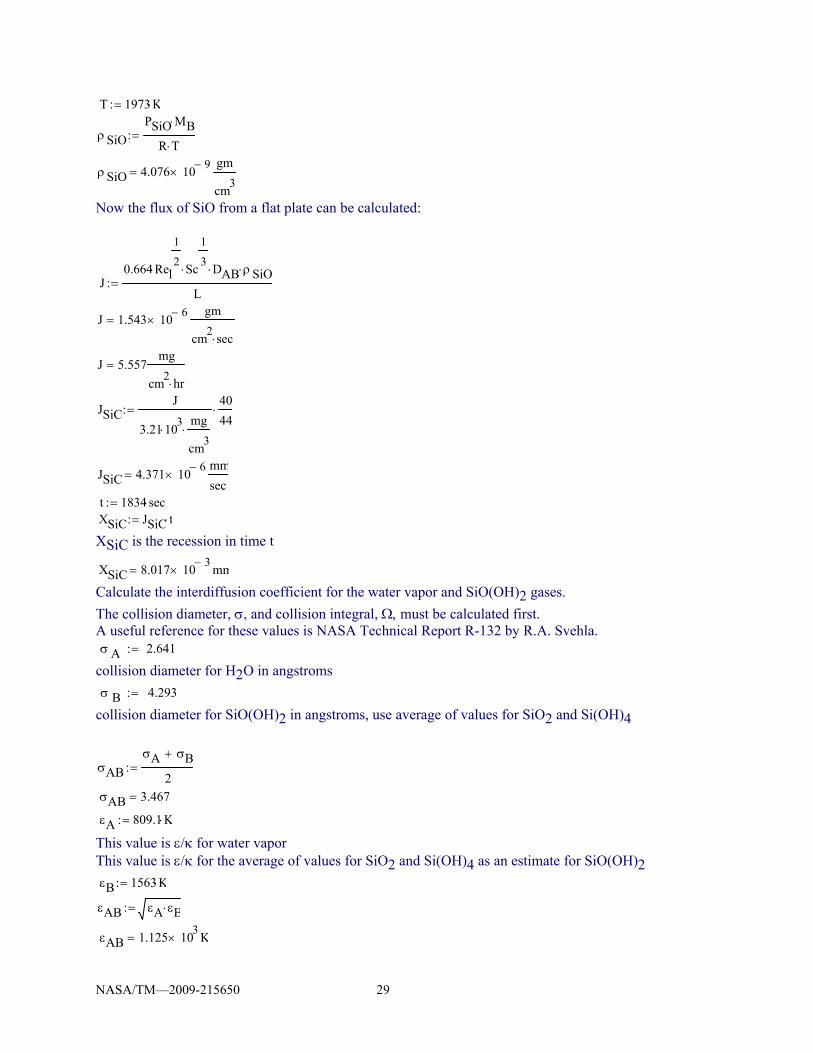
Now the flux of SiO from a flat plate can be calculated:

XSiC is the recession in time t

Calculate the interdiffusion coefficient for the water vapor and SiO(OH)2 gases.

The collision diameter, , and collision integral, must be calculated first. A useful reference for these values is NASA Technical Report R-132 by R.A. Svehla.

collision diameter for H2O in angstroms

collision diameter for SiO(OH)2 in angstroms, use average of values for SiO2 and Si(OH)4

This value is /for water vapor This value is /for the average of values for SiO2 and Si(OH)4 as an estimate for SiO(OH)2

T 1973 K

SiO

PSiO MB

R T

SiO 4.076 109

gm

cm3

J0.664 Rel

1

2 Sc

1

3 DAB SiO

L

J 1.543 106

gm

cm2

sec

J 5.557mg

cm2

hr

JSiCJ

3.21 103

mg

cm3

40

44

JSiC 4.371 106

mm

sec

t 1834 secXSiC JSiC t

XSiC 8.017 103

mm

A 2.641

B 4.293

AB

A B

2

AB 3.467

A 809.1 K

B 1563 K

AB A B

AB 1.125 103

K

NASA/TM—2009-215650 30

is then picked from a table on p. 20 of Mass Transfer by Sherwood et al. based on the value of T`. :=1.127 The interdiffusion coefficient can now be calculated using the Chapman-Enskog Equation:

The values are all entered without units here because the equation is formulated with the constant .0018583 and P(atm), T(K), (angstroms), M(gm/mole).

T:=1973 P:=0.34

The Schmidt number can now be calculated:

The pressure and concentration of SiO(OH)2 are now needed: Nate's transpiration data for SiO(OH)2 are

used in conjunction with the Allendorf Cp data.

The concentration of SiO(OH)2 is then:

T'T

AB

T' 1.754

M A 18

M B 78

DAB .00185831

MA

1

MB T

3

21

P AB2

DAB 9.246

DAB 9.246cm

2

sec

P 0.34 atmT 1973 K

M 18gm

mole

R82.06 cm

3 atm

mole K

P M

R T

3.78 105

gm

cm3

Sc

DAB

Sc 1.878

PSiOOH2 1.77 106

atm

MB 78gm

mole

T 1973 K

NASA/TM—2009-215650 31

Now the flux of SiO(OH)2 from a flat plate can be calculated:

XSiC is the recession in time t

Calculate the interdiffusion coefficient for the water vapor and Si(OH)4 gases.

The collision diameter, , and collision integral, must be calculated first. A useful reference for these values is NASA Technical Report R-132 by R.A. Svehla.

collision diameter for H2O in angstroms

collision diameter for Si(OH)4 in angstroms

use data for SiF4 as best approximation

This value is /for water vapor

This value is /for SiF4 as an approximation for Si(OH)4

SiOOH2

PSiOOH2 MB

R T

SiOOH2 8.527 1010

gm

cm3

J0.664 Rel

1

2 Sc

1

3 DAB SiOOH2

L

J 2.289 107

gm

cm2

sec

J 0.824mg

cm2

hr

JSiCJ

3.21 103

mg

cm3

40

61

JSiC 4.677 107

mm

sec

t 1834 secXSiC JSiC t

XSiC 8.578 104

mm

A 2.641

B 4.880

AB

A B

2

AB 3.76

A 809.1K

B 171.9 K

AB A B

AB 372.94K

NASA/TM—2009-215650 32

is then picked from a table on p. 20 of Mass Transfer by Sherwood et al. based on the value of T`. :=0.8336 The interdiffusion coefficient can now be calculated using the Chapman-Enskog Equation:

The values are all entered without units here because the equation is formulated with the constant .0018583 and P(atm), T(K), (angstroms), M(gm/mole). MB:=96 T:=1973 P:=0.34

The Schmidt number can now be calculated:

The pressure and concentration of Si(OH)4 are now needed:

This information is based on Nate's paper with data input to FactSage. Material temp of 1973K was used to calculate PSi(OH)4

The concentration of Si(OH)4 is then:

Now the flux of Si(OH)4 from a flat plate can be calculated:

T'T

AB

T' 5.29

M A 18

DAB .00185831

MA

1

MB T

3

21

P AB2

DAB 10.437

DAB 10.437cm

2

sec

Sc

DAB

Sc 1.664

PSiOH4 1.4 106

atm

MB 96gm

mole

T 1973 K

SiOH4

PSiOH4 MB

R T

SiOH4 8.301 1010

gm

cm3

J0.664 Rel

1

2 Sc

1

3 DAB SiOH4

L

NASA/TM—2009-215650 33

XSiC is the recession in time t

J 2.416 107

gm

cm2

sec

J 0.87mg

cm2

hr

JSiCJ

3.21 103

mg

cm3

40

96

JSiC 3.136 107

mm

sec

t 1834 secXSiC JSiC t

XSiC 5.752 104

mm

NASA/TM—2009-215650 35

Appendix D.—Assumptions Made in Calculating Recession With Equation (1) Several assumptions have been made in this calculation. First, the density of the gas boundary layer is

calculated assuming it is entirely water vapor. This is a reasonable assumption since the combustion gases are composed of 60 percent water vapor.

Second, it is assumed that the gas boundary layer is laminar. This is also a reasonable assumption. The Reynolds number has been calculated for each condition (see Appendix C) and compared to Re = 3105, the criterion for transition from laminar to turbulent flow. In all cases, the Reynolds number is less than this quantity for most of the length of the panel. Surface roughness is expected to result in more turbulent flow. If the gas boundary layer is turbulent the major effect on the calculated recession is to increase the exponent on the Reynolds number from 0.5 to 0.7, thus an increased dependence on the gas velocity is expected. However, the overall recession is only expected to increase by a small factor, so trends indicated by the calculated recession based on laminar flow are expected to hold true.

Third, in the calculation of the interdiffusion coefficient of the volatile Si-O-H species in the gas boundary layer, assumptions have been made about the force constants: collision diameter and /k of the Si-O-H gas molecules. The force constants for SiO(g) are found in Svehla’s report (SVE62) and the collision integral is interpolated using the tabulated values in Hirschfelder (HIR54). The force constant data for SiF4(g) from Svehla are used as an approximation for Si(OH)4(g). This is expected to be a fairly good assumption since OH groups are often compared to halide groups. The average collision diameter and /k data of SiF4(g) and SiO2(g) from Svehla are used for SiO(OH)2(g). This may not be a good assumption, however, it is known that gas phase diffusion coefficients do not vary much, so inaccuracies in the collision diameter and /k for SiO(OH)2(g) are expected to have very little effect on the overall calculated recession rates.

NASA/TM—2009-215650 37

Appendix E.—Estimation of Oxide Thickness on SiC SAA P&W. SiC recession in cell 22 Estimate silica thickness for case 3 and case 4, where silica is assumed to be on the surface of the SiC. First estimate parabolic oxidation rate, kp assuming:

Deal and Grove temperature dependence for transport of H2O through silica, 68 kJ/mol Using data from Opila, J.Am.Ceram.Soc. 82 [3] 625 (1999) - oxidation rate of SiC in water vapor at 1400 °C, PH2O = 0.9 atm, kp = 3.510–3 mg2/cm4 h First convert kp to units of silica thickness growth rate:

this expression is in mg2/cm4h

this expression is in 2/h solve for pre-exponential

in J/K mol T:=1673 in degrees K

now at 1700C:

this expression is in 2/h Now assume that kp varies with PH2O to the exponent of 1 (molecular diffusion of H2O in silica). The value just determined was in 0.9 atm PH2O

this value is valid for kp at 1 atm PH2O Case 3, Ptotal = 0.34 atm Case 4, Ptotal = 2.10 atm at MR=6, PH2O = 0.6*Ptotal

kp3:=kpwo.pH2O_3

kp1400 3.5 103 168

kp1400 0.588

R 8.314472

kTpokp1400

exp68000

R T

kTpo 78.062

T 1973

kp1700 kTpo exp68000

R T

kp1700 1.237

kpwokp1700

0.9

kpwo 1.374

pH2O_3 0.6 0.34pH2O_3 0.204

pH2O_4 1.26

kp3 0.28

pH2O_4 0.6 2.10

NASA/TM—2009-215650 38

Now assume oxidation rates are one order of magnitude larger due to impurities in the combustion environment: kp3real:=kp3.10

this expression is in 2/h kp4real:=kp4.10

this expression is in 2/h Calculate limiting oxide thickness, xL=kp/2kl. kl from previous calculations assuming silica is on the surface of SiC These recession rates are due to SiO, Si(OH)4 and SiO(OH)2 formation. Units in microns/1834 sec.

converted to microns/h. Converting from SiC recession to SiO2 recession (factor of 2).

now the limiting oxide thickness for each case:

These expressions for xL are in microns. So for both xL3 and xL4, an oxide thickness of 20 to 40 nm is predicted on the surface of the SiC. This assumes parabolic oxidation. At these nm oxide thicknesses, oxidation may be linear and reaction limited rather than diffusion limited. These thicknesses represent an upper bound.

now the time to reach steady state is calculated

Units are in hours, steady state is reached in three seconds for tL3 and even faster for tl4.

kp4 1.731

kp3real 2.803

kp4real 17.311

kl3 9.46( ) 23600

1834

kl3 37.138

kl4 119( ) 23600

1834

kl4 467.176

xL3kp3real

2 kl3

xL3 0.038

xL4kp4real

2 kl4

xL4 0.019

tl3kp3real

2 kl32

tl3 1.016 103

tL4kp4real

2 kl42

tL4 3.966 105

kp4 kpwo pH2O_4

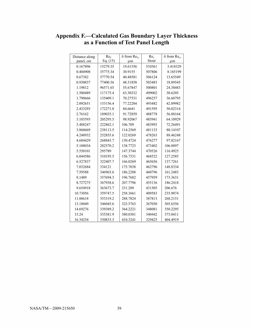
NASA/TM—2009-215650 39

Appendix F.—Calculated Gas Boundary Layer Thickness as a Function of Test Panel Length

Distance along

panel, cm ReL

Eq. (15) from ReL,

m Rex

Stout from Rex,

m

0.167896 15279.35 19.61556 510361 3.418329

0.404908 35775.34 30.9155 507806 8.185199

0.67382 57770.54 40.48581 506124 13.65549

0.930837 77400.36 48.31858 503483 18.89545

1.19812 96571.65 55.67847 500801 24.38483

1.500489 117175.4 63.30332 499002 30.6205

1.790666 135409.1 70.27531 496257 36.60795

2.092651 153156.4 77.22204 493482 42.89982

2.433293 172271.8 84.6641 491595 50.02314

2.76162 189035.1 91.72859 488778 56.88164

3.103593 205295.5 98.92067 485941 64.10929

3.488247 222862.1 106.709 483993 72.26491

3.860669 238113.5 114.2569 481133 80.14107

4.248932 252855.6 122.0269 478263 88.46248

4.684429 268843.7 130.4724 476277 97.82167

5.108034 282570.2 138.7723 473402 106.8897

5.550101 295789 147.3744 470526 116.4925

6.044586 310195.5 156.7331 468522 127.2585

6.527837 322407.7 166.0269 465656 137.7261

7.032684 334121 175.7038 462796 148.8334

7.59588 346965.6 186.2288 460796 161.2483

8.1489 357694.3 196.7682 457959 173.3631

8.727275 367938.6 207.7796 455136 186.2418

9.654918 363673.7 231.209 431505 206.676

10.73056 359747.5 258.3661 409583 235.9074

11.88618 353319.2 288.7824 387813 268.2151

13.18049 346045.6 323.5763 367050 305.6556

14.69276 339389.2 364.2221 348081 350.2295

15.24 335381.9 380.0381 340442 373.0411

16.34254 330833.3 410.3241 329425 404.4919

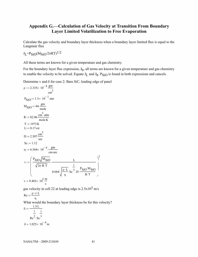
NASA/TM—2009-215650 41

Appendix G.—Calculation of Gas Velocity at Transition From Boundary Layer Limited Volatilization to Free Evaporation

Calculate the gas velocity and boundary layer thickness when a boundary layer limited flux is equal to the Langmuir flux

JL=PSiO(MSiO/2RT)1/2

All these terms are known for a given temperature and gas chemistry.

For the boundary layer flux expression, Jb, all terms are known for a given temperature and gas chemistry

to enable the velocity to be solved. Equate JL and Jb. PSiO is found in both expressions and cancels.

Determine v and for case 2: Bare SiC, leading edge of panel

gas velocity in cell 22 at leading edge is 2.5x103 m/s

What would the boundary layer thickness be for this velocity?

2.335 104

gm

cm3

PSiO 1.3 101

atm

MSiO 44gm

mole

R 82.06cm

3atm

mole K

T 1973 KL 0.17 cm

D 2.507cm

2

sec

Sc 1.121

6.564 104

gm

cm sec

vPSiO MSiO

2 R T

L

0.664 L

Sc

1

3 D

PSiO MSiO

R T

2

v 9.483 105

m

s

Re v L

1.5 L

Re

1

2Sc

1

3

1.025 106

m

NASA/TM—2009-215650 42

For a boundary layer thickness of 1 micron, the Langmuir flux applies. This is independent of the pressure of the volatile species, and depends primarily on the boundary layer properties.

Ap

pen

dix

H.—

Cal

cula

ted

Par

tial

Pre

ssu

res

of S

i-O

-H V

olat

ile

Sp

ecie

s as

a F

un

ctio

n o

f P

anel

Su

rfac

e T

emp

erat

ure

. Kri

kor

ian

(K

RI7

0) D

ata

for

SiO

(OH

)(g)

(N

ot R

ecom

men

ded

)

T

AB

LE

H1.

—C

AL

CU

LA

TE

D P

AR

TIA

L P

RE

SSU

RE

S O

F Si

-O-H

VO

LA

TIL

E S

PE

CIE

S A

T M

R =

6, P

= 0

.34

AT

M,

AS

A F

UN

CT

ION

OF

PA

NE

L S

UR

FA

CE

TE

MP

ER

AT

UR

E

TC

Si

(OH

)4

SiO

(OH

) Si

O(O

H)2

Si

O

Ptot

al

X

Si(O

H)4

,Pe

rcen

t X

SiO

(OH

),Pe

rcen

t X

SiO

(OH

)2,

Perc

ent

XSi

O,

Perc

ent

Xto

tal

1200

5.

51E

-07

8.71

E-0

8 2.

71E

-09

2.35

E-1

0 6.

02E

-07

85

.02

14.4

9 0.

45

0.04

1.

00E

+00

1250

6.

22E

-07

2.52

E-0

7 6.

29E

-09

9.95

E-1

0 8.

82E

-07

70

.57

28.6

0 0.

71

0.11

1.

00E

+00

1300

6.

97E

-07

6.82

E-0

7 1.

38E

-08

3.83

E-0

9 1.

40E

-06

49

.93

48.8

1 0.

99

0.27

1.

00E

+00

1350

7.

76E

-07

1.73

E-0

6 2.

90E

-08

1.36

E-0

8 2.

55E

-06

30

.43

67.9

0 1.

14

0.53

1.

00E

+00

1400

8.

58E

-07

4.15

E-0

6 5.

80E

-08

4.44

E-0

8 5.

11E

-06

16

.79

81.2

1 1.

13

0.87

1.

00E

+00

1450

9.

43E

-07

9.47

E-0

6 1.

15E

-07

1.35

E-0

7 1.

07E

-05

8.

85

88.8

1 1.

08

1.27

1.

00E

+00

1500

1.

03E

-06

2.06

E-0

5 2.

06E

-07

3.86

E-0

7 2.

22E

-05

4.

64

92.6

9 0.

93

1.74

1.

00E

+00

1550

1.

12E

-06

4.28

E-0

5 3.

69E

-07

1.04

E-0

6 4.

54E

-05

2.

47

94.4

2 0.

81

2.29

1.

00E

+00

1600

1.

21E

-06

8.57

E-0

5 6.

41E

-07

2.65

E-0

6 9.

02E

-05

1.

35

95.0

1 0.

71

2.94

1.

00E

+00

1650

1.

31E

-06

1.65

E-0

4 1.

08E

-06

6.41

E-0

6 1.

74E

-04

0.

75

94.9

4 0.

62

3.68

1.

00E

+00

1700

1.

40E

-06

3.08

E-0

4 1.

77E

-06

1.48

E-0

5 3.

26E

-04

0.

43

94.4

8 0.

54

4.55

1.

00E

+00

T

AB

LE

H2.

—C

AL

CU

LA

TE

D P

AR

TIA

L P

RE

SSU

RE

S O

F Si

-O-H

VO

LA

TIL

E S

PE

CIE

S A

T M

R =

6, P

= 2

.10

AT

M,

AS

A F

UN

CT

ION

OF

PA

NE

L S

UR

FA

CE

TE

MP

ER

AT

UR

E

TC

Si

(OH

)4

SiO

(OH

) Si

O(O

H)2

Si

O

Ptot

al

X

Si(O

H)4

,Pe

rcen

t X

SiO

(OH

),Pe

rcen

t X

SiO

(OH

)2,

Perc

ent

XSi

O,

Perc

ent

Xto

tal

1200

2.

10E

-05

2.17

E-0

7 1.

67E

-08

2.35

E-1

0 2.

13E

-05

98

.90

1.02

0.

08

0.00

1.

00E

+00

1250

2.

37E

-05

6.27

E-0

7 3.

89E

-08

9.95

E-1

0 2.

44E

-05

97

.27

2.57

0.

16

0.00

1.

00E

+00

1300

2.

66E

-05

1.69

E-0

6 8.

54E

-08

3.83

E-0

9 2.

84E

-05

93

.72

5.97

0.

30

0.01

1.

00E

+00

1350

2.

96E

-05

4.30

E-0

6 1.

79E

-07

1.36

E-0

8 3.

41E

-05

86

.82

12.6

2 0.

52

0.04

1.

00E

+00

1400

3.

27E

-05

1.03

E-0

5 3.

58E

-07

4.44

E-0

8 4.

35E

-05

75

.35

23.7

3 0.

82

0.10

1.

00E

+00

1450

3.

60E

-05

2.35

E-0

5 6.

89E

-07

1.35

E-0

7 6.

03E

-05

59

.63

39.0

0 1.

14

0.22

1.

00E

+00

1500

3.

93E

-05

5.12

E-0

5 1.

28E

-06

3.86

E-0

7 9.

21E

-05

42

.68

55.5

2 1.

38

0.42

1.

00E

+00

1550

4.

28E

-05

1.06

E-0

4 2.

28E

-06

1.04

E-0

6 1.

53E

-04

28

.04

69.7

9 1.

50

0.68

1.

00E

+00

1600

4.

63E

-05

2.13

E-0

4 3.

96E

-06

2.65

E-0

6 2.

66E

-04

17

.42

80.1

0 1.

49

1.00

1.

00E

+00

1650

4.

99E

-05

4.11

E-0

4 6.

67E

-06

6.42

E-0

6 4.

74E

-04

10

.54

86.7

0 1.

41

1.35

1.

00E

+00

1700

5.

36E

-05

7.66

E-0

4 1.

09E

-05

1.48

E-0

5 8.

45E

-04

6.

34

90.6

1 1.

29

1.76

1.

00E

+00

NASA/TM—2009-215650 43

NASA/TM—2009-215650 45

Appendix I.—Photos of Borosilicate Glass Droplets on Panel 388 Tracked for Liquid Velocity Measurements. Flow is From Left to Right. The Horizontal

Black Lines in the Images are Artifacts of the Software

Figure I1.—Drops A (left) and D (right), 8.903 sec. Figure I2.—Drop B, 9.307 sec.

Figure I3.—Drop C, 8.500 sec.

REPORT DOCUMENTATION PAGE Form Approved

OMB No. 0704-0188 The public reporting burden for this collection of information is estimated to average 1 hour per response, including the time for reviewing instructions, searching existing data sources, gathering and maintaining the data needed, and completing and reviewing the collection of information. Send comments regarding this burden estimate or any other aspect of this collection of information, including suggestions for reducing this burden, to Department of Defense, Washington Headquarters Services, Directorate for Information Operations and Reports (0704-0188), 1215 Jefferson Davis Highway, Suite 1204, Arlington, VA 22202-4302. Respondents should be aware that notwithstanding any other provision of law, no person shall be subject to any penalty for failing to comply with a collection of information if it does not display a currently valid OMB control number. PLEASE DO NOT RETURN YOUR FORM TO THE ABOVE ADDRESS.

1. REPORT DATE (DD-MM-YYYY) 01-12-2009

2. REPORT TYPE Technical Memorandum

3. DATES COVERED (From - To)

4. TITLE AND SUBTITLE Integrated High Payoff Rocket Propulsion Technology (IHPRPT) SiC Recession Model

5a. CONTRACT NUMBER

5b. GRANT NUMBER

5c. PROGRAM ELEMENT NUMBER

6. AUTHOR(S) Opila, E., J.

5d. PROJECT NUMBER

5e. TASK NUMBER

5f. WORK UNIT NUMBER WBS 599489.02.07.03.02.04.01

7. PERFORMING ORGANIZATION NAME(S) AND ADDRESS(ES) National Aeronautics and Space Administration John H. Glenn Research Center at Lewis Field Cleveland, Ohio 44135-3191

8. PERFORMING ORGANIZATION REPORT NUMBER E-16962

9. SPONSORING/MONITORING AGENCY NAME(S) AND ADDRESS(ES) National Aeronautics and Space Administration Washington, DC 20546-0001

10. SPONSORING/MONITOR'S ACRONYM(S) NASA

11. SPONSORING/MONITORING REPORT NUMBER NASA/TM-2009-215650

12. DISTRIBUTION/AVAILABILITY STATEMENT Unclassified-Unlimited Subject Category: 24 Available electronically at http://gltrs.grc.nasa.gov This publication is available from the NASA Center for AeroSpace Information, 443-757-5802

13. SUPPLEMENTARY NOTES

14. ABSTRACT SiC stability and recession rates were modeled in hydrogen/oxygen combustion environments for the Integrated High Payoff Rocket Propulsion Technology (IHPRPT) program. The IHPRPT program is a government and industry program to improve U.S. rocket propulsion systems. Within this program SiC-based ceramic matrix composites are being considered for transpiration cooled injector faceplates or rocket engine thrust chamber liners. Material testing under conditions representative of these environments was conducted at the NASA Glenn Research Center, Cell 22. For the study described herein, SiC degradation was modeled under these Cell 22 test conditions for comparison to actual test results: molar mixture ratio, MR (O2:H2) = 6, material temperatures to 1700 °C, combustion gas pressures between

0.34 and 2.10 atm, and gas velocities between 8,000 and 12,000 fps. Recession was calculated assuming rates were controlled by volatility of thermally grown silica limited by gas boundary layer transport. Assumptions for use of this model were explored, including the presence of silica on the SiC surface, laminar gas boundary layer limited volatility, and accuracy of thermochemical data for volatile Si-O-H species. Recession rates were calculated as a function of temperature. It was found that at 1700 °C, the highest temperature considered, the calculated recession rates were negligible, about 200 µm/h, relative to the expected lifetime of the material. Results compared favorably to testing observations. Other mechanisms contributing to SiC recession are briefly described including consumption of underlying carbon and pitting. A simple expression for liquid flow on the material surface was developed from a one-dimensional treatment of the Navier-Stokes Equation. This relationship is useful to determine under which conditions glassy coatings or thermally grown silica would flow on the material surface, removing protective layers by shear forces. The velocity of liquid flow was found to depend on the gas velocity, the viscosity of gas and liquid, as well as the thickness of the gas boundary layer and the liquid layer. Calculated flow rates of a borosilicate glass coating compared well to flow rates observed for this coating tested on a SiC panel in Cell 22.15. SUBJECT TERMS SiC; Recession; Combustion

16. SECURITY CLASSIFICATION OF: 17. LIMITATION OF ABSTRACT UU

18. NUMBER OF PAGES

50

19a. NAME OF RESPONSIBLE PERSON STI Help Desk (email:help@sti.nasa.gov)

a. REPORT U

b. ABSTRACT U

c. THIS PAGE U

19b. TELEPHONE NUMBER (include area code) 443-757-5802

Standard Form 298 (Rev. 8-98)Prescribed by ANSI Std. Z39-18