Integrated Geophysical Methods Applied to Geotechnical … and Resources/Near Surface... · Integrated Geophysical Methods Applied to Geotechnical and ... Penetration Test) ... if
65
Integrated Geophysical Methods Applied to Geotechnical and Geohazard Engineering: From Qualitative to Quantitative Analysis and Interpretation Dr. Koichi Hayashi The 2015 Near Surface Asia Pacific Conference 2015/07/08 1
Integrated Geophysical Methods Applied to Geotechnical and
Geohazard Engineering: From Qualitative to Quantitative
Analysis and Interpretation
Dr. Koichi HayashiThe 2015 Near Surface Asia Pacific Conference
2015/07/08
1
Outline
• Uncertainty in geophysical processing• Integrated Geophysical Methods• Application of the Integrated
Geophysical Methods • Conclusions
2
Presenter
Presentation Notes
This is outline of my talk. At first, I will introduce uncertainty in geophysical processing. Next, I will show the concept of integrated geophysical method to improve the problem of uncertainty and increase accuracy and reliability of geophysical methods. Third, I will show several application examples of the integrated geophysical method.
Outline
• Uncertainty in geophysical processing• Integrated Geophysical Methods• Application of the Integrated
Geophysical Methods • Conclusions
3
Presenter
Presentation Notes
In this talk, I do not focus on particular method. I would like to discuss general idea on the limitation of geophysical methods and how can we solve these limitations practically. One of the most important limitations of geophysical methods is uncertainty. Today, I would like to show the uncertainty in geophysical methods and introduce the concept of integrated geophysical ,method in order to solve uncertainty.
Cause of uncertainty or error • Geophysical issues
Non-uniquenessModel parameterizationDependence on initial conditionsConstraints
• Engineering issuesDifference of resolutionDifference between geophysical properties and engineering parameters
4
Presenter
Presentation Notes
At first, I would like to discuss the uncertainly of geophysical method. There are several causes of uncertainly during processing or inversion, such as non-uniqueness, model parameterization, dependence on initial condition and constraints. Today, I would like to show typical non-uniqueness for example. In addition to these mathematical issues in geophysical methods, we usually apply geophysics to other engineering problems in practical applications and we have to consider other issues, such as resolution and difference between geophysical and engineering properties.
Non-uniqueness in refraction data analysis
Traveltime curves for 2-layer model0
2
4
6
8
10
12
14
16
18
20
0 500 1000 1500 2000 2500
Dept
h(m
)
Velocity (m/sec)
5
Presenter
Presentation Notes
Here is an example of non-uniqueness in seismic refraction method. If we have a two-layer velocity model, traveltime curves looks like as a figure on the right. There is a direct arrival and a refracted arrival.
Non-uniqueness in refraction data analysis
Traveltime curves for 3-layer model0
2
4
6
8
10
12
14
16
18
20
0 500 1000 1500 2000 2500
Dept
h(m
)
Velocity (m/sec)
6
Presenter
Presentation Notes
Now, we have a special three layer model. This is a traveltime curve. We have direct, refraction from a second layer and refraction from a third layer. We can see that the first arrivals are only direct and the refraction from the third layer. The refraction from second layer will never be the first arrival.
Non-uniqueness in refraction data analysis
0
2
4
6
8
10
12
14
16
18
20
0 500 1000 1500 2000 2500
Dept
h(m
)
Velocity (m/sec)
Traveltime curves for 50-layer model
7
Presenter
Presentation Notes
This is a 50 layer model. And its traveltime curves. We can see that only direct arrival and refraction from 50th layer can be seen as the first arrival and the refraction from second to 49th layers will never be the first arrival.
Non-uniqueness in refraction
Uncertainty
8
Presenter
Presentation Notes
This is a comparison of five different velocity models with two, three, four, five and 50 layers. If we compare the first arrivals of these five velocity model, they are completely same. It implies that if we have only first arrival traveltime curve, we can never distinguish these five velocity models. This is a typical example of non-uniqueness. We usually call this kind of error uncertainty.
Uncertainty due to the difference in resolution
Observed data from passive surface wave method
S-wave velocity model
Comparison with Seismic Log9
Uncertainty
Presenter
Presentation Notes
I would like to talk about the uncertainly from a little bit different point of view. As I mentioned before, we have to consider different issues when we apply geophysical methods to other engineering or scientific areas. The difference of the resolution is big issue if we compare different methods. For example, this is a dispersion curve obtained by a surface wave method. This is a velocity model obtained by an inversion. The model is represented by 10 layers and S-wave velocity and thickness were estimated. We have a seismic log at the site. This is a comparison of S-wave velocity obtained by the surface wave method and seismic log. What do you think about this comparison? If we take some averaging for the seismic log, both profiles agrees very well. However, if we compare the S-wave velocity at some particular depth, for example 150m, S-wave velocity from the surface wave method is 600m/sec, seismic log may be 400 or 1000m/sec. there may be a large error or uncertainly. Like this seismic log, natural ground is generally very heterogeneous and complicated. Contrary, most geophysical method performed on the ground surface cannot delineate such small scale heterogeneity. We have to recognize this difference in resolution.
Differences between geophysical properties and engineering parameters
Geophysical properties do not directly relate to engineering properties !
10
Comparison of S-wave velocity and N-value (obtained by Standard Penetration Test)
Uncertainty
Presenter
Presentation Notes
Another important issue is what kind of property or parameters we need. Geophysical methods generally give us geophysical properties, such as P-wave velocity, S-wave velocity and resistivity. In contrast, engineering needs different parameters, such as Cohesion and internal friction angle, grain size distribution, sand or clay or gravel, and permeability. We usually have to estimate these engineering parameters from geophysical properties. There is no physical relationship between these values and this estimation generally includes large uncertainty. For example, this is a relationship between N-value obtained by standard penetration test and S-wave velocity. We can see there is large uncertainty.
Outline
• Uncertainty in geophysical processing• Integrated Geophysical Methods• Application of the Integrated
Geophysical Methods • Conclusions
11
Presenter
Presentation Notes
Conclusions so far, individual geophysical method is not enough for engineering purposes. How can we improve geophysical methods? This lecture will focus on integrated use of geophysical methods to improve the applicability of geophysical methods.
What is the Integrated Geophysical Methods?
• Several different geophysical methods are used together
• Geotechnical or geological investigation results are combined with geophysical results
• Different sets of information with a variety of resolutions and dimensions are combined
• Engineering parameters are estimated from geophysical properties
• Change the analysis from qualitative to quantitative 12
Presenter
Presentation Notes
What is the integrated geophysical methods? This is the summary. Several different geophysical methods are used together. Geotechnical or geological investigation results are combined with geophysical results. Different sets of information with a variety of resolutions and dimensions are combined. Engineering parameters are estimated from geophysical properties. Change the analysis from qualitative to quantitative.
Why do we need several different geophysical methods ?
Typicalengineering parameters
Geophysical properties
P-velocity S-velocity Resistivity
Groundwater level
○ × △
Stiffness △ ○ ×
Soil type △ △ △
Permeability × △ △
13
○:Good relationship△: Some relationship×: No relationship
Presenter
Presentation Notes
Why do we need several different geophysical methods ? In engineering site investigation, engineers typically need there parameters. Groundwater level, stiffness of soil, such as hard or soft, and soil type, such as sand, clay or gravel. How can we estimate these values from geophysical data? For example, P-wave velocity is sensitive to ground water, but there is no direct relationship to stiffness and soil type. S-wave velocity has direct relationship to the stiffness of soil, but no relationship to groundwater. Resistivity has no relationship to stiffness and some relationship to groundwater and soil type. But these relationships are not direct. Clearly, one geophysical method is not enough. We have to combine several methods together. This is a basic concept of the integrated geophysical method.
Provide a-priori information to constrain initial model
0
2
4
6
8
10
12
14
16
18
20
0 500 1000 1500 2000 2500
Dept
h(m
)
Velocity (m/sec)
2 layer
3 layer
4 layer
5 layer
50 layer
0
2
4
6
8
10
12
14
16
18
20
0 10 20 30 40 50
Dep
th (
m)
N-Value
2 layer model
0
2
4
6
8
10
12
14
16
18
20
0 10 20 30 40 50
Dep
th (
m)
N-Value
50 layer model
Blow counts (N-value) obtained by Standard Penetration Test
14
Presenter
Presentation Notes
The integrated geophysical method does not only mean integrating several geophysical methods. Other investigation method, such as geotechnical investigations can be combined. For example, most geophysical methods are non-uniqueness and a-priori information and constraint are very important in the inversion. For example, refraction method has non-uniqueness as I mentioned before. However, if we have some drilling logs, we can use them for a-priori information. For example this is N-value, obtained by standard penetrating test. If we have this N-value, there is clear boundary, it is better to choose 2 layer model. If we have this N-Value, there is no clear boundary and the N-value increasing with depth, it is better to choose smooth, such as 50 layer model. This is very simple idea but many geophysicists tend to analyze geophysical data without other information.
Combine methods with different resolutions and dimensions
Geophysical section Boring
Laboratory Test
15
Presenter
Presentation Notes
Another important concept of the integrated geophysical is combining different methods with different resolution and dimension. This is a resistivity section obtained by the resistivity method. And we have boring logs. Clearly the resolution of boring is much better than the geophysical methods and boring gives as much detailed information. We generally get soil or rock samples from boring and do laboratory tests. This is a grain size distribution. The resolution of laboratory tests is much better than boring and it gives us much detailed information. Question is which method is the best? There is no answer. We have to combine all together.
Flood control along a river
Boring
BoringBoring
16
Presenter
Presentation Notes
Let me think about flood control along a river. River is long continuous object. Of course, we cannot perform the boring continuously. However, levee breaks at some particularly place. In order to evaluate the levee continuously, we have to combine different methods together, Boring, Laboratory tests, and Geophysical methods. This is a very important concept of the integrated geophysical methods.
Outline
• Uncertainty in geophysical processing• Integrated Geophysical Methods• Application of the Integrated
Geophysical Methods • Conclusions
17
Presenter
Presentation Notes
From here, I would like to show actual examples of the integrated geophysical methods.
East Japan Earthquake and levee collapse (2011)
2011 Earthquake
Kanto plain
200kmNeed to detect weakened levees
without visible damage 18
Presenter
Presentation Notes
The first example is the levee investigation after 2011 East Japan Earthquake. The earthquake occurred 2011, magnitude was 9. The Kanto plain is placed several hundred kilometers away from ruptured area. Many levees were damaged. Like these photos. The problem is the levee loosened or damaged by the earthquake without visible damage.
Integrated Geophysical Method for evaluation of levee damage
5km
Survey line length = 160km
19
Presenter
Presentation Notes
This is a north-east portion of Kanto area. We applied the integrated geophysical method to many levees in the area. Yellow lines are survey lines. Total length of investigated levees was 160km.
Data acquisition
Surface wave surveyCapacitively-coupled
resistivity survey
20
Presenter
Presentation Notes
We applied a surface wave method using a land-streamer. And a capacitively coupled resistivity. We applied two methods to 160km of levee and total length of geophysical survey was 320km.
10408015030060015003000700042.2K 42.4K 42.6K 42.8K 43.0K 43.2KBoring A
Boring B
10 20 30 40 50
5
10
15
BS 0.6BS
2.0BS
3.5BS
5.3BS 6.1CH 7.2CH 8.0
GS
11.7
FS
15.7M-S
17.8S
10 20 30 40 50
5
10
15
BS 2.7
BS
6.7SM
7.9M-O
9.4Pt
10.8MS 11.8MO 12.4MS
14.1C 14.3M 15.1GF 15.4GS
17.0CH
Levee body
FoundationA database of the results from 160km of geophysical sections with boring logs was used for statistical analysis 21
Presenter
Presentation Notes
These are examples of sections, S-wave velocity and resistivity sections. This is only 1km and we have 160 km similar geophysical sections in this project. We put all 160km of geophysical sections together with bring logs to database in order to perform statistical analysis.
S-wave velocity and resistivity for levee safety
• From the modified Archie’s equation, the resistivity of soil mainly indicates the soil type.
• S-wave velocity is mainly affected by the stiffness or porosity.• The safety of levees can be evaluated by the S-wave velocity
and resistivity.
S-wave velocity
Resistivity
High
LowLow High
Soil type
Clay, Silt
Sand, Gravel
S-wave velocity
Resistivity
High
LowLow High
Safety
Safe (hard, tight, silty, clayey )
Danger (soft, loose, sandy, gravel)
Stiffness (degree of compaction)
High(hard, tight)
Low(soft, loose)
22
Large permeability
Small permeability
Presenter
Presentation Notes
This is a concept of levee safety evaluation based on S-wave velocity and resistivity. From the modified Archie’s equation, resistivity of soil mainly indicates soil type. High resistivity indicates sand or gravel and low resistivity indicates silt or clay. S-wave velocity is mainly affected by shear strength or porosity. High S-wave velocity indicates hard ground and low S-wave velocity indicates soft and loose ground. From the levee safety point of view, loose, soft and sandy or gravel levee is more danger than hard, tight and silty, clay levees. Safety of levees can be evaluated by S-wave velocity and resistivity.
S-wave velocity (m/s)
Vs, resistivity, in-situ and laboratory tests
0.001
0.01
0.1
1
10
10 100 1000 10000
20%
Gra
in s
ize
(mm
)
Resistivity (ohm-m)
N-V
alue
(SPT
)
N<3
VS<135m/s
Sand and gravel
ρ>200 ohm-m
Gravel
Sand
Clay
23
Presenter
Presentation Notes
I will show some examples of the statistical analysis using the database. This is a relationship between S-wave velocity and N-Value obtained from the standard penetrating tests. In Japan, the N-value has been conventionally used in levee safety evaluation and the relationship between S-wave velocity and N-Value is very important. For example, N-value less than 3 is usually considered as very loose soil. From this relationship, we define that S-wave velocity less than 135m/sec is loose soil. This is a relationship between resistivity and 20 % grain size. Color represents soil type, and blue, yellow and orange indicate clay, sand and gravel respectively. From rule of thumb, we defined that the soil its 20% grain size is larger the 0.03mm is sand and gravel. It corresponds to the resistivity of 200 ohm-m. Then, we will use the S-wave velocity of 135m/sec and the resistivity of 200 ohm-m for levee safety evaluation.
Cross-plot of Vs and resistivity
10
100
1000
75 100 125 150 175 200 225
Res
istiv
ity (o
hm-m
)
S-wave velocity (m/sec)
Danger
Safe
Vs =135 m/sR
esis
tivity
= 2
00 O
hm-m
24
Presenter
Presentation Notes
We made a cross-plot of S-wave velocity and resistivity using all 160 km of geophysical data. Difference of color and symbol indicates different river. As I mentioned before, top-left corner, high resistivity and low S-wave velocity area is more danger than bottom-right corner, low resistivity and high S-wave velocity. We set a threshold of S-wave velocity 135m/sec that corresponds to N-value less than 3. And a threshold of resistivity 200ohm-m that corresponds to a boundary between sand and clay. In conclusion, the data in this top left corner is relatively danger compared with rest of data.
Cross-plot analysis
Above groundwater
Below groundwater
S-wave velocity
Resistivity
Dangerous
25
Presenter
Presentation Notes
This is an example of actual processing. At first, we have S-wave velocity and resistivity sections. Next, we made cross-plots of S-wave velocity and resistivity. Sometimes, we divide data into two groups, above and below ground water, because groundwater may have large effect on the resistivity. We set the thresholds and evaluate the safety of levee from geotechnical point of view. Finally, we return the data on the cross-plots to the section. These red areas are relatively danger compared with rest of section.
Integrated Geophysical Method for evaluation of levee damage
5km
Survey line length = 160km
26
Using the Integrated Geophysical Method (including geophysics, borehole data, and levee maintenance records), we could identify the damaged sections from a very long levee.
Presenter
Presentation Notes
This is conclusions of our levee safety evaluation. We did 160 km of the integrated geophysical method in Kanto plain. And select three relatively danger portion, about 4km out of 160km based on cross-plot analysis. This one, about the 500m of levee is danger. This one about 2km. And this one, about 1.5km. In conclusion, we could select relatively danger portion from very long levee using the integrated geophysical method. I would like to note that, this is not only from geophysics. We drew this conclusion together with borehole data, laboratory tests and levee maintenance record as well.
Earthquake engineering
Long period
Short period
Buildings and foundation
Source characteristics
Propagation path effects
Local site effects
27
Basin Edge Effect
Presenter
Presentation Notes
Next, I change the subject to the earthquake engineering. The earthquake is very complex problem. We have source. We need to understand the source. Seismic waves generated at the source are propagating the earth. We need to understand the propagation path. We have many kinds of waves, for example, short period and long period. Generally, seismic velocity at the near-surface is slow and seismic waves are amplified. This is called local site effect. However, most of damages from the earthquake are due to buildings and foundation. Seismic ground motion itself does not kill people. We have to understand the buildings and foundation. Today, I would like to talk about the local site effect.
Local site amplification
20km
My officeSan Andreas Fault(Earthquake 1906)
Pacific plate
North American plate
Calaveras Fault
Hayward Fault
30-year probabilities of magnitude 6.7 or greater earthquakes on the Hayward and Calaveras Faults have been estimated at 31% and 7%, respectively 28
M6.0 Earthquake (2014/8/24)
Pacific plate
North American plate
Presenter
Presentation Notes
Our investigation site is the San Francisco Bay Area. I am currently working at Geometrics office in San Jose. The San Francisco Bay Area is placed on the plate boundary between The Pacific plate and North American Plate. The Pacific plate is moving north-west and North American plate is moving south-east direction. Here a plate boundary that is defined as San Andreas Fault that is running here. It generated the San Francisco earthquake at 1906. Its magnitude was 7.8. As the plate boundary, The San Andreas Fault takes charge of only one third of all displacement. Other faults, such as Hayward Fault and Calaveras Fault share the displacement of plate motion. According to the USGS, United States of Geological Survey, 30-year probabilities of magnitude 6.7 or greater earthquakes on the Hayward and Calaveras Faults have been estimated at 31% and 7%, respectively. It is very big probability and my office is very close to Hayward Fault and this is my problem.
Basin edge effectSeismic ground motion can be locally
amplified at the edge of a tectonic basin.
Bedrock
Sedimentary layers
Tectonic basinConverted surface waves
Surface ground motionBasin Edge
Effect
Hayward Fault
29
Presenter
Presentation Notes
Purpose of this investigation is studying so called the basin edge effect that seismic ground motion can be locally amplified at the edge of tectonic basin. Here is the Hayward Fault and west side of Hayward Fault is a Tectonic Basin where bedrock is very deep. If seismic waves get into this model, it will be amplified at the tectonic basic because there are thick low S-wave velocity layers. At the edge of basin, body waves may convert into surface waves and it propagates horizontal direction. Together with the amplification due to the low S-wave velocity layer, the converted surface waves may also increase surface ground motion at the tectonic basin side. This is so called the Basin Edge Effect.
Site of investigation
Diablo Range
San Francisco Bay Area
30
Presenter
Presentation Notes
This is a site of investigation. This is the Hayward Fault and this is the Calaveras Fault. There is a mountain, called Diablo Range, between Hayward and Calaveras Faults. Here, bedrock is almost exposure. Left hand side of the Hayward Fault is San Francisco Bay Area where bedrock depth is deep. In order to investigate S-wave velocity model of this area, we performed seismic tests at ten sites.
Surface wave methods• Multichannel Analysis of Surface Waves
(MASW)
• Passive Surface Wave Survey Using geophones in a Linear Array (Linear-MAM)
• Two-station Spatial Autocorrelation (2ST-SPAC)
46 to 92m (48 receivers)
46 to 92m (48 receivers)
Depth < 20m
10m < Depth < 100m
50m < Depth < 2000m31
4.5Hz geophones
4.5Hz geophones
Broadband accelerometers
Presenter
Presentation Notes
We performed three surface wave methods at each site in order to estimate shallow to deep S-wave velocity profiles. The first is multi-channel analysis of surface waves. We put 48 geophones and hit the ground by a sledge hammer. We observe high frequency phase velocities to estimate shallow S-wave velocity profiles, down to a depth of 20m. The next is passive surface wave method. We use same geophone array and observed ambient noise 10 to 20 minutes. It observed middle frequency range of phase velocity to estimate intermediate depth, down to 100m. Finally, we put two broad band accelerometers with variable separations. We call it a two-station SPAC. Recorded the ambient noise 10 minutes to one hour and obtained low frequency phase velocities. Its penetration depth is down to 2000m. We integrated all three methods together and estimate S-wave velocity from surface to a depth of several kilometers.
Comparison of dispersion curves
0
200
400
600
800
1000
1200
1400
1600
1800
0.1 1 10 100
Phas
e ve
loci
ty (m
/sec
)
Frequency (Hz)
MASW
Linear-MAM
2ST-SPACWavelength=10km
1km
500m
200m
100m
50m
20m10m
2km
5km
MASW (Active)Linear-MAM(Passive with geophones)
2ST-SPAC(Passive with broadband sensor )
32
Presenter
Presentation Notes
This is the example of dispersion curves. MASW using active sources gave us the phase velocity higher than 10Hz. Passive measurements using geophones (Linear-MAM) gave us 3 to 10Hz. Two-station SPAC gave us the frequency range of 0.2 to 4Hz. We can see that three dispersion curves agree with each other and the two-station SPAC gave us extremely low frequency and long wave length phase velocities. It implies that the two-station SPAC method give us very deep S-wave velocity information compared with other methods.
Schematic S-wave velocity modelacross the faults
700-800
1000-1500 1500-2000
Study 2D effect on surface ground motion
33
Presenter
Presentation Notes
This is a result of investigation, S-wave velocity profiles obtained at ten sites are shown. Here is the Hayward Fault and here is the Calaveras Fault. Let me focus on shallow bedrock, S-wave velocity is 700 to 800 m/sec. A depth to the bedrock is about 100m at the left hand side of the Hayward Fault. In contrast the bedrock is almost exposure between the Hayward and the Calaveras Faults. Let me focus on intermediate bedrock, S-wave velocity is 1000 to 1500 m/sec. A depth to the bedrock is 400 to 700m at the left hand side of the Hayward Fault. In contrast, the depth to bedrock is very shallow, less than 100m between two faults. S-wave velocity of the deepest bedrock is about 1500 to 2000m/sec. Depth to the bedrock is 1000 to 2000m at the west side of the Hayward Fault. Let me focus on the Hayward Fault, we can see that the bedrock depth, 1000 to 1500m/sec for example, changes about 400m. Here after, I would like to study effect of this two dimensional structure on surface seismic ground motion.
This is the two dimensional S-wave velocity model across the Hayward Fault. Here is the Hayward Fault. We input plane SH wave at the bottom of model. It propagates to upper direction.
This is a wave propagation calculated by a 2D finite difference method. The plane SH wave propagates to upper direction and reflected at the surface and back to lower direction. At the Hayward fault, other waves were generated and propagate to left hand side horizontally. They are surface waves, Love waves in this case.
I recorded the ground motion at the surface. Here is the Hayward Fault. This is a surface ground motion across the Hayward Fault. This is a direct wave. And we can see that other waves were generated at the Hayward Fault and propagates to left hand side. They are surface waves, Love waves.
We evaluate the effect of 2D structure quantitatively. I calculated the amplification, it is the amplitude of surface ground motion compared with the amplitude at the bedrock in frequency domain. This is a result of 1D calculation which does not include the effect of 2D ground motion. Vertical axis is frequency and color indicates the amplification. Blue to green indicates small amplitude and yellow to red indicates large amplitude. At the left hand side of the Hayward Fault, we can see that the amplitude is large at frequency of about 1Hz. It is about 4 times compared with bedrock.
Bedrock depth changes at least 400m across the Hayward Fault, and it may cause large local amplification (4 to 6 times greater than bedrock). The impact of this so-called basin edge effect must be taken into account at least several kilometers away from the Hayward Fault.
Presenter
Presentation Notes
Let me compare 1D and 2D calculation. They look basically same. However, at the left hand side of the Hayward Fault, amplitude of 2D calculation around the frequency of 1Hz is much larger than 1D. Let me focus on the frequency of 1Hz. At the distance of 1500 and 2500m for example, amplitude is 5 to 6 times larger than bedrock. In conclusions, bedrock depth changes at least 400m across the Hayward Fault, and it may cause local large amplification. It is 4 to 6 times compared with bedrock. We have to take account this effect of 2D structure, so called the basin edge effect, at least several kilometers away from the Hayward Fault.
Investigation site
Investigation site
Inuvik
Arctic Circle
40
Presenter
Presentation Notes
I would like to move up my presentation to further north, the North-west territory of Canada. Name of the city is Inuvik. It locates within the Arctic Circle.
Inuvik
Temperature at Inuvik
2 degrees
0.5 degrees
World average
41
Presenter
Presentation Notes
This project is the global warming. This is average temperature of all Earth and temperature increase 0.5 degree in last 50 years. This is the historical temperature at Inuvik. Average temperature increases about 2 degrees in last 50 years in Inuvik and it clearly shows that global warming is more serious at Inuvik compared with rest of the world.
Inuvik Airport on permafrost
About 1800m
Subsidence Zones
A B
42
The airport is on permafrost (permanently frozen soil)
Presenter
Presentation Notes
Our investigation site was the airport at Inuvik. The airport is on the permafrost which is permanently frozen soil. There was subsidence on the runway. It subsided about 50cm. This is another subsidence on taxiway.
Ground temperature of permafrost
WinterSpring
SummerFall
Summer
Runway ground temperatures to a depth of 540 cm at
Tasiujaq, Northern Quebec, 2004-2005Allard et al., 2007
Time
Depth
Frozen
Melted About 1m
Ground surface
Active layer is the top layer of soil that thaws during the summer and freezes again during the autumn.
MeltedActive layer
43
Tem
pera
ture
(C) 0 degree
Depth
Presenter
Presentation Notes
The problem is the permafrost at this site. This is the example of temperature change below a runway. The depth is from 90 cm to 5m. We can see that temperature in shallow depth raises more than 0 degree in summer time. This is the schematic diagram of permafrost. Shallow surface of the permafrost melt or thaw in summer and freeze in winter. This zone is called active layer. In the Inuvik area, people said that the thickness of active layer is about 1m.
Active layer in Inuvik Airport
Typical soil type
Depth
Time
Embankment
Peat (soft)
Stony, clayey silt
Global warming
Frozen
Active layer thickness may increase
Engineering problem?
3m
5m
How deep the active layer? What is the effect on runway subsidence?
Seismic and resistivity methods44
Presenter
Presentation Notes
Here is the problem of active layer in Inuvik. At the Inuvik airport, the thickness of runway embankment is about 3m and there is a peat layer below the embankment. These embankment and peat layer are permafrost and basically frozen. The embankment melts on summer time. It is not the problem. As the global warming progress, Thickness of active layer increases, If it reaches to peat layer, there may be engineering problems. The purpose of this investigation is investigating how deep the active layer and evaluating its effect on runway subsidence. We applied seismic and resistivity methods to study this problem.
Data acquisition
45
Presenter
Presentation Notes
We performed the data acquisition in middle of June. This is the airport under operation and we could not do the data acquisition at daytime. Then we did the field work at night time. Here is the arctic region and the Sun never sets in June. This is middle of night; we do not need to prepare lights for fieldwork.
Comparison of waveformNormal zone Subsidence zone (A)
They are examples of shot gathers used in surface wave analysis. We can see clear first arrivals and surface waves. A left hand side is a shot gather at no subsidence and right hand side is a shot gather at a subsidence. We can see that the apparent velocity of surface waves at subsidence zone are slower and frequency is lower. I converted these shot gathers to frequency and phase velocity domain. Blue color indicates large amplitude and it goes to dispersion curve. Let me focus on a frequency of 30 Hz, phase velocity is about 800 m/sec in the shot gather at no subsidence and 400 m/sec at the shot gather at subsidence zone. There is a big difference of phase velocity at the subsidence zone.
Temperature (C)
Res
istiv
ity (O
hm-m
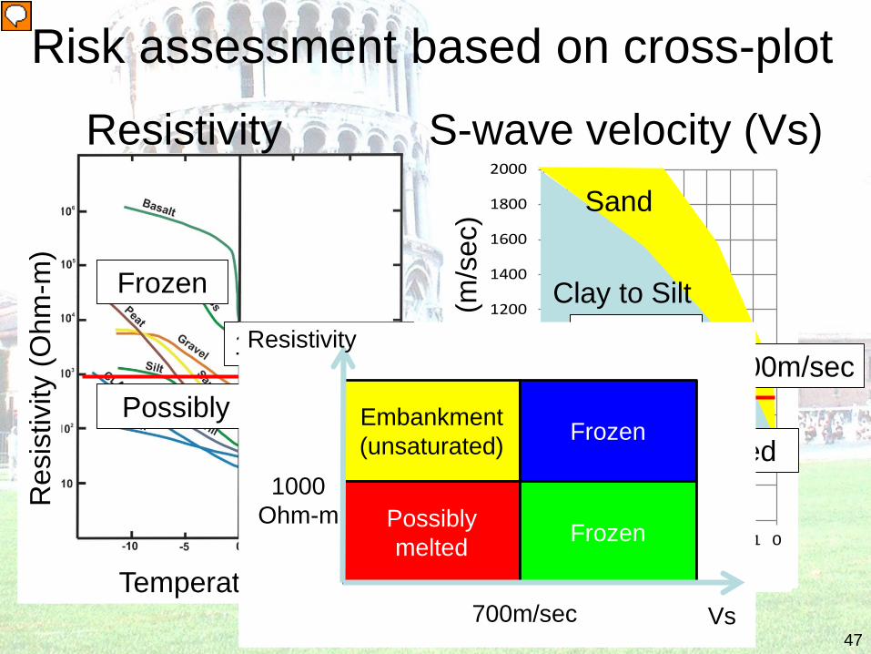
)Risk assessment based on cross-plot
0
200
400
600
800
1000
1200
1400
1600
1800
2000
-10 -9 -8 -7 -6 -5 -4 -3 -2 -1 0
S-wa
ve ve
locit
y (m
/sec
)
Tempelature (C)
Clay to Silt
Sand
Resistivity S-wave velocity (Vs)
1000 Ohm-m700m/sec
Frozen
Frozen
Possibly meltedPossibly Melted
47
Temperature (C)
S-w
ave
velo
city
(m
/sec
)
Embankment(unsaturated)
Possiblymelted
Frozen
Frozen
1000 Ohm-m
700m/sec Vs
Resistivity
Presenter
Presentation Notes
I am going to figure out the cause of subsidence in terms of integrated geophysical method. A left hand side is a relationship between resistivity and temperature, a right hand side is a relationship between S-wave velocity and temperature. We can see that the relationship very depends on soil type. But in spite of soil type, both resistivity and S-wave velocity increase with temperature decrease. We defined thresholds, between frozen and melted, resistivity of 1000 ohm-m and S-wave velocity of 700m/sec. They are boundary of frozen and possibility melted. We made this cross-plot using based on the thresholds of resistivity 1000ohm-m and S-wave velocity 700m/sec and soil condition. Definitely, this area, S-wave velocity is slower than 700 m/sec and resistivity is less than 1000 ohm-m, is possibly melted.
Subsidence at the site is due to the melted permafrost, probably a peat layer, beneath the embankment. The results of the Integrated Geophysical Method gave us the area of possibly melted soils.
Presenter
Presentation Notes
We have S-wave velocity and resistivity sections. Applied the cross-plot of 1000 ohm-m 700m/sec , to these sections. This is a cross-plot. I return the cross-plot analysis to the section. Red color indicates soil possibly melted. We can see that thickness of melted layer is large in this area. It agrees with subsidence zone. In conclusions, subsidence at the site is due to the melted permafrost, probably peat layer, beneath the embankment. The results of integrated geophysical method gave us the area of possibly melted soils.
Tidal flats
49
Tidal flats or mud flats are large beach that are exposed by tidal action
• Tidal flats or mudflats are important ecosystems.
• They usually support a large population of wildlife.
• The maintenance of tidal flats is important in preventing coastal erosion.
• However, tidal flats worldwide are under threat from predicted sea level rises, land claims for development, dredging due to shipping purposes, and chemical pollution.
Presenter
Presentation Notes
Final example is tidal flats or mud flats. Tidal flats or mud flats are large beach that are exposed by tidal action, like this photograph. Tidal flats or mudflats are important ecosystems. They usually support a large population of wildlife. The maintenance of tidal flats is important in preventing coastal erosion. However, tidal flats worldwide are under threat from predicted sea level rises, land claims for development, dredging due to shipping purposes, and chemical pollution.
Tidal Flat at San Francisco Bay1850 2000
Hydro-geologists and engineers try to reproduce and restore tidal flats so it is important to understand their characteristic soil conditions. This can be done using the Integrated Geophysical Method.
50
Presenter
Presentation Notes
This is a tidal flat at San Francisco Bay Area. This is a map of tidal flat at 1850, green area was tidal flats. This is a map at 2000. You can see that the most tidal flats were disappeared in 150 years. Hydro-geologists and engineers try to reproduce and restore tidal flats so it is important to understand their characteristic soil conditions. This can be done using the Integrated Geophysical Method.
Tidal flat investigations
12 : Japan2 : Canada
51
Presenter
Presentation Notes
We applied the integrated geophysical method to many tidal flats. 12 tidal flats in Japan and two tidal flats in Canada. Let me compare some results.
Surface wave method at tidal flatLow tideHigh tide
52
Presenter
Presentation Notes
We applied the surface wave method. This is the high tide. This is the low tide at the same place. When the tide is low, we did measurements using a land streamer. Put a seismograph on a cart, we need some beach parasol. And we hit the ground by a sledge hammer and generate seismic waves.
Sandy tidal flat
Oita
Bar
Trough
53
Presenter
Presentation Notes
There are many kind of tidal flats consisting of different soil types. At first, this is an example of sandy tidal flats. The site is Oita, Japan. It looks like this. This is the S-wave velocity section obtained from a surface wave method. Velocity is increasing with depth. We measured surface topography and there is clear oscillation, Called bar and trough. This oscillation is common in sandy tidal flats. This is near surface, average of top 50 cm, S-wave velocity. We can see clear oscillation like topography. High S-wave velocity agrees with high topography and low S-wave velocity agrees with low elevation.
Muddy tidal flat
Kumamoto
54
Presenter
Presentation Notes
Next is a muddy tidal flat, called mudflat. The site is Kumamoto, Japan. It looks like this. It is a very soft tidal flat and people cannot walk on the surface. We used special boat for data acquisition. This is an S-wave velocity section. Top 3 to 4 m is extremely slow; S-wave velocity is less than 50 m/sec. This is near surface, average of top 50 cm, S-wave velocity. There is no oscillation like sandy tidal flat.
Tidal flat in Vancouver
Vancouver3km
Muddy
Sandy
Muddy
55
Presenter
Presentation Notes
Last example is Vancouver, Canada. The site is here. It looks like this. It is a very wide tidal flat. Survey line is more than 3 km from coast to offshore. This is an S-wave velocity section. Difference of elevation is more than 3m. This is a near surface S-wave velocity. The tidal flat consists of both sandy and muddy part. The sandy part is high velocity and muddy part is low velocity. There is clear oscillation at sandy part and no oscillation at muddy part. We can see clear relationship between S-wave velocity and soil type and topography of tidal flats.
S-wave velocity
Ground level
Vane shear test
Where can we find clams at beach?
Bar Trough
Trough Bar
56
Presenter
Presentation Notes
We are going to discuss a relationship between soil condition and ecology. Here, I would like to study where we can find clams at beach. This is an example of tidal flats. We can see clear oscillation of topography. It is called bar and Trough. This is a comparison of S-wave velocity, topography and Vane shear test. Let me focus on the bar and trough. At the trough, S-wave velocity is low, elevation is low, and shear strength is low. In contrast, S-wave velocity is high, elevation is high and shear strength is high at the bar. We can see clear relationship between S-wave velocity, topography and shear strength.
Where can we find clams at beach?
Clams can dive
Sassa & Watabe (2009)
Clams dive into sandSoft sand
Hard sand
S-wave velocity
Ground level
Vane shear test
Trough
Trough (slow velocity and low shear strength) is better for clams.
57
Presenter
Presentation Notes
Next, we will investigate the relationship between shear strength and where clams would like to live. This is an experiment of clams. We made soil samples with different stiffness or shear strength. In soft sand, clams can dive into sand and they can live in the sand. In hard sand, clams cannot dive into the sand. Clams prefer soft sand. We made the soil samples with different shear strength and different density, and observed clams can dive into the sand or not. This is the result. In spite of density, clams can dive into the sand when shear strength is less than 0.3. This is the comparison of S-wave velocity and shear strength I mentioned before. For example, here is a trough. At the trough, S-wave velocity is low, elevation is low, and shear strength is low. Trough (slow velocity and low shear strength) is better for clams.
Where can we find clams at beach?
Trough
Go to the troughs or do a surface wave survey and find the low S-wave velocity areas !
58
Presenter
Presentation Notes
Finally, the answer to the question is; Go troughs or Do surface wave method and find low S-wave velocity area.
Conclusions• The “Near-Surface” provides benefits from nature that
are indispensable in our lives• Near surface geophysics relates to many other
science and engineering areas and understanding such related areas is very important
• Most geophysical analyses are essentially non-unique, and it is very difficult to obtain unique and reliable solutions without uncertainty from an individual geophysical method
• It is very important to understand the limitation of geophysical methods and to combine all available information
59
Presenter
Presentation Notes
The “Near-Surface” provides benefits from nature that are indispensable in our lives. Near surface geophysics relates to many other science and engineering areas and understanding such related areas is very important. Most geophysical analyses are essentially non-unique, and it is very difficult to obtain unique and reliable solutions without uncertainty from an individual geophysical method. It is very important to understand the limitation of geophysical methods and to combine all available all information.
Acknowledgements Society of Exploration Geophysicists Geometrics, Inc. OYO Corporation California State University East Bay Department of Transportation, Government of the
Northwest Territories, Canada Public Works Research Institute, Japan Port Airport Research Institute, Japan Washington State Department of Natural Resources Louisiana State university
60
Acknowledgements• Mony Geophysical Exploration• Nippon Geophysical Prospecting• Suncoh consultant• Nippon Koei• Prof. Jon Tunnicliffe, Univ. of Auckland• Prof. Alex Becker, Univ. of California, Berkeley• Prof. Lothar Schrott of Univ. of Salzburg• Dr. Patrick Finlay of EBA
61
SEG Membership
SEG Digital Library - full text articles Technical Journals in Print and Online Networking Opportunities Receive Membership Discounts on: Continuing Education Courses Publications (35% off list price)
Workshops and Meetings
Join Online http://seg.org/join S E G m a t e r i a l s a r e a v a i l a b l e t o d a y !
62
Student Opportunities Student Chapters available
Student Chapter Book Program SEG/Chevron Student Leadership Symposium Challenge Bowl