integer-valued garch processes - mat.uc.pt · duced in gonçalves et al (2015), that enlarges and...

Pré-Publicações do Departamento de Matemática

Universidade de Coimbra

Preprint Number 18�39

SIGNED COMPOUND POISSON

INTEGER-VALUED GARCH PROCESSES

E. GONÇALVES AND N. MENDES-LOPES

Abstract: We propose signed compound Poisson integer-valued GARCH processesfor the modelling of the di�erence of count time series data. We investigate the the-oretical properties of these processes and we state their ergodicity and stationarityunder mild conditions. We discuss the conditional maximum likelihood estimatorwhen the series appearing in the di�erence are INGARCH with geometric distribu-tion and explore its �nite sample properties in a simulation study. Two real dataexamples illustrate this methodology.

Keywords: Integer-valued time series, GARCH model, compound Poisson distri-butions.

AMS Subject Classification (2010): 62M10.

1. Introduction

The practical relevance of count time series has led to the development ofseveral class of integer-valued models in order to better describe and capturethe main characteristics of this kind of data. Among these classes, we high-light that of the compound Poisson INGARCH (CP-INGARCH) models, intro-duced in Gonçalves et al (2015), that enlarges and uni�es the main INGARCHprocesses present in literature and has the ability of capturing simultaneouslycharacteristics of overdispersion and conditional heteroscedasticity, in a generaldistributional context.Some papers emerged in the literature in recent years (a.e. Karlis and Nt-

zoufras, 2006, 2009; Koopman et al, 2014) have shown the interest of signedinteger-valued time series de�ned by the Skellam distribution, which is con-structed as di�erences in pairs of Poisson counts independent or not. Suchmodels allow us to describe, for example, the di�erences over time in the num-ber of accidents, catastrophes, or people contracting certain epidemic diseasein two cities, two world regions, or two populations.Several studies have shown that Poissonian models have some limitations

to describe counting data, particularly because this kind of data usually has

Received October 1, 2018.

1

2 E. GONÇALVES AND N. MENDES-LOPES

overdispersion characteristics, which are not captured by Poissonian distribu-tions but by others such as negative binomial (NB), Neyman-type A, general-ized Poisson (see a.e. Weiÿ, 2009; Zhu, 2011, 2012; Gonçalves et al, 2015) allof them included in the supra referred CP-INGARCH models. Therefore, toconsider the di�erences of general counting models have obviously theoreticaland practical interest.Following this idea we present here a Z-valued counting model de�ned as the

di�erence between two general independent CP-INGARCH processes, whichwill allow to describe in practice such kind of data, even when the phenomenaunder study has di�erent distributional behavior in each situation considered(in that di�erence). We observe that our proposal di�ers from those in whichmodels to adjust time series with Z-values are based on thinning operators,a subject where Kim and Park (2008) was pioneering; a good review of thesethinning operators models is presented in Scotto et al (2015).For sake of technical simplicity, we start with the study of a bivariate model

de�ned by two independent CP-INGARCH processes from which the di�erencemodel, that is the signed CP-INGARCH one, is constructed. The main proba-bilistic properties of weak and strict stationarity and ergodicity are deduced fora wide class of these kind of bivariate models. After we consider any measurablefunction of the marginal processes and in what concerns the statistical anal-ysis we concentrate our study in the estimation by the conditional maximumlikelihood method of a particular case of signed geometric INGARCH model,that is, that corresponding to a bivariate model whose marginal processes areparticular NB-INGARCH ones.The remainder of the paper is organized as follows. In Section 2 we recall the

class of CP-INGARCH models by presenting its de�nition and construction aswell as its main subclasses. The bivariate process is introduced in Section 3.Properties of stationarity and ergodicity are developed and, in particular, nec-essary and su�cient conditions of weak and strict stationarity are established.The signed CP-INGARCH model is de�ned in Section 4. For the particularcase of the signed geometric INGARCH processes, we develop in this Sectionthe conditional maximum likelihood estimator of the model parameter vector.The performance of the conditional likelihood estimator in �nite samples isevaluated via simulation experiments. We observe that with our models, wecan compare a temporal phenomenon in di�erent periods (su�ciently distantto assume independence) but also compare it in di�erent situations; we illus-trate it by discussing the monthly counts of poliomyelitis cases recorded in the

SIGNED CP INGARCH PROCESSES 3

United States in two periods as well as another application related to the num-ber of Olympic medals won by Swiss and Dutch athletes over all time. Someconcluding remarks end the paper.

2. Preliminairies

Let us recall the de�nition of Compound Poisson integer-valued GARCHmodel introduced in Gonçalves et al (2015) as well as some results that arerelevant for the study presented in next Sections.Let X = (Xt, t ∈ Z) be a stochastic process with values in N0 and, for any

t ∈ Z, let X t−1 be the σ−�eld generated by {Xt−j, j ≥ 1}.

De�nition 2.1 (CP-INGARCH(p,q) model). The process X is said to satisfya Compound Poisson INteger-valued GARCH model with orders p and q (p,q ∈ N) if, ∀t ∈ Z, the characteristic function of Xt|X t−1 is given by{

ΦXt|Xt−1(u) = exp

{i λtϕ′t(0)

[ϕt(u)− 1]}, u ∈ R

E(Xt|X t−1) = λt = α0 +∑p

j=1 αjXt−j +∑q

k=1 βkλt−k(1)

for some constants α0 > 0, αj ≥ 0 (j = 1, ..., p), βk ≥ 0 (k = 1, ..., q),and where (ϕt, t ∈ Z) is a family of characteristic functions on R, X t−1-measurable associated to a family of discrete laws with support N0 and �nitemean. i denotes the imaginary unit.

As ϕt, t ∈ Z, is the characteristic function of a discrete law with support N0

and �nite mean, the derivative of ϕt at u = 0, ϕ′t(0), exists and is nonzero.

In the previous de�nition, if βk = 0, k = 1, ..., q, the CP-INGARCH(p, q)model is simply denoted CP-INARCH(p).

Remark 2.1. (1) As the conditional distribution of Xt is a discrete com-pound Poisson law with support N0 then, ∀t ∈ Z and conditionally toX t−1, Xt can be identi�ed in distribution as

Xtd=

Nt∑j=1

Xt,j, (2)

where Nt follows a Poisson law with parameter λ∗t = i λt/ϕ′t(0), and

Xt,1,..., Xt,Ntare discrete independent random variables, with support

contained in N0, independent of Nt and having characteristic functionϕt with �rst derivative at zero, that is, with �nite mean. We note that


the characteristic function ϕt being X t−1-mensurable may be a randomfunction. This means that ϕt may depend on the previous observationsof the process.

(2) Let us consider the polynomialsA(L) = α1L+ ...+ αpL

p and B(L) = 1− β1L− ...− βqLq,where L is the backshift operator. To ensure the existence of the inverseof B(L) we suppose that the roots of B(z) = 0 lie outside the unitcircle which, for non-negative βj, is equivalent to

∑qj=1 βj < 1. Under

this assumption, the conditional expectation of the model (1) may berewritten in the form

B(L)λt = α0 + A(L)Xt ⇔ λt = α0B−1(1) +B−1(L)A(L)Xt

that is, with B−1(L)A(L) =∑∞

j=1 ψjLj,

λt = α0B−1(1) +

∞∑j=1

ψjXt−j,

which expresses a CP-INARCH(+∞) representation of the model (1).(3) The process X satisfying the model (1) is �rst order stationary if and

only if∑p

i=1 αi+∑q

j=1 βj < 1. Under this condition, the processes (Xt)and (λt) are both �rst order stationary and

E(Xt) = E(λt) =α0

1−∑p

i=1 αi −∑q

j=1 βj.

(4) If ϕt is deterministic, t ∈ Z, and independent of t, there is a strictlyand weakly stationary and ergodic process that satis�es the model (1),if and only if

∑pi=1 αi +

∑qj=1 βj < 1.

(5) The sub-class of CP-INGARCH models with ϕt deterministic and inde-pendent of t is still quite vaste including, among others. the INGARCH(Ferland et al, 2006), Negative-Binomial DINARCH (Xu et al, 2012),Generalized Poisson INGARCH (Zhu, 2012), Neyman type-A and GE-OMP2 (Gonçalves et al, 2015) INGARCH models.

3. Bivariate model

3.1. De�nition.Let X = (Xt, t ∈ Z) be a bivariate stochastic process, Xt = (X1,t, X2.t) ,

where X1 = (X1,t, t ∈ Z) and X2 = (X2,t, t ∈ Z) are univariate processes and,for any t ∈ Z, let X t−1 be the σ−�eld generated by {Xt−j, j ≥ 1}. If X1 satisfy


a CP-INGARCH(p, q) model and X2 satisfy a CP-INGARCH(p, q) model andif, for any t ∈ Z, X1,t e X2.t are independent relatively to the law conditionedby X t−1, then the characteristic function of Xt|X t−1 is, for any t ∈ Z, given by

ΦXt|Xt−1

(u, v) = exp{i Mt

ϕ′t(0)[ϕt(u)− 1]

}exp

{i Mt

ϕ′t(0)[ϕt(v)− 1]

}, (u, v) ∈ R2

E(X1,t|X1,t−1) = Mt = α0 +∑p

j=1 αjX1,t−j +∑q

k=1 βkMt−k,

E(X2,t|X2,t−1) = Mt = α0 +∑p

j=1 αjX2,t−j +∑q

k=1 βkM t−k,

(3)for some constants α0 > 0, αj ≥ 0 (j = 1, ..., p), βk ≥ 0 (k = 1, ..., q),

α0 > 0, αj ≥ 0 (j = 1, ..., p), βk ≥ 0 (k = 1, ..., q) and where (ϕt, t ∈ Z)and (ϕt, t ∈ Z) are two families of characteristic functions on R, X1,t−1 andX2,t−1−measurable, respectively, each one associated to a family of discretelaws with support N0 and �nite mean.We assume in what follows the hypothesis

H1 :

q∑k=1

βk < 1 and

q∑k=1

βk < 1. (4)

Introducing the polynomialsA(L) = α1L+ ...+ αpL

p and B(L) = 1− β1L− ...− βqLq,A(L) = α1L+ ...+ αpLp and B(L) = 1− β1L− ...− βqLq,

we may ensure the existence of the following representations for Mt and Mt

Mt = α0B−1(1) +

∑∞j=1 ψjX1,t−j, Mt = α0B

−1(1) +∑∞

j=1 ψjX2,t−j,

where ψj (resp., ψj) is the coe�cient of zj in the Maclaurin expansion of

A(z)/B(z) (resp., A(z)/B(z)), that is, B−1(L)A(L) =∑∞

j=1 ψjLj (resp.,

B−1(L)A(L) =∑∞

j=1 ψjLj).

3.2. First and second order stationarity.The process X is �rst order stationary if and only if

∑pi=1 αi +

∑qj=1 βj < 1

and∑p

i=1 αi +∑q

j=1 βj < 1. Under these conditions, the processes (X1,t) and


(Mt) are both �rst order stationary, as well as (X2,t) and (Mt), and we have

E(X1,t) = E(Mt) = µ =α0

1−∑p

i=1 αi −∑q

j=1 βj,

E(X2,t) = E(Mt) = µ =α0

1−∑p

i=1 αi −∑q

j=1 βj.

The study of the second order stationarity of CP- INGARCH models wasundertaken in Gonçalves et al (2015) under the condition

H2 : −iϕ′′

t (0)

ϕ′t (0)

= υ0 + υ1λt,

with υ0 ≥ 0, υ1 ≥ 0, not simultaneously zero. The stated results are valuablefor a quite general subclass including both random and deterministic charac-teristic functions ϕt; in particular, they apply to the INGARCH (Ferland et al,2006), NB-INARCH (Zhu, 2011), NB-DINARCH (Xu et al, 2012), GeneralizedPoisson INGARCH (Zhu, 2012), Neyman type-A INGARCH models and alsoto all the models where the ϕt functions are determinist and independent of t.This study apply naturally to the bivariate model Xt = (X1,t, X2.t) since thematrices of variances-covariances, ΓXt

(h) , h = 0, 1, 2, ..., are given by

ΓXt(h) =

[Cov (X1,t+h, X1,t) Cov (X1,t+h, X2,t)Cov (X1,t+h, X2,t) Cov (X2,t+h, X2,t)

]=

[Cov (X1,t+h, X1,t) 0

0 Cov (X2,t+h, X2,t)

]=

[ΓX1,t

(h) 00 ΓX2,t

(h)

],

due to the independence of X1 and X2.From Theorems 2 of Gonçalves et al (2015) and 3.1 of Gonçalves et al (2016),

a necessary and su�cient condition of weak stationarity of processes (X1,t) and(X2.t) and consequently of (Xt) is deduced.We refer, for example, that for a �rst order stationary CP-INGARCH(1,1)

model verifying H2, a necessary and su�cient condition of weak stationarity is(α1 + β1)

2 +υ1α21 < 1.We also note that the autocovariances of a second order

CP-INGARCH(p, q) process X and those of λ (respectively, Γ and Γ) verifythe linear equations


Γ (h) =

p∑j=1

αjΓ (h− j) +

min(h−1,q)∑k=1

βkΓ (h− k) +

q∑k=h

βkΓ (h− k) , h ≥ 1,

Γ (h) =

min(h,p)∑j=1

αjΓ (h− j) +

p∑j=h+1

αjΓ (j − h) +

q∑k=1

βkΓ (h− k) , h ≥ 0,

assuming that∑q

k=h βkΓ (h− k) = 0 if h > q and∑p

j=h+1 αjΓ (j − h) =0 if h > p. In particular, the autocovariances of a weakly stationary CP-INGARCH(1,1) are given by

Γ (h) =α1 (1− β1 (α1 + β1)) (α1 + β1)

h−1

1− (α1 + β1)2 + α2

1

Γ (0) , h ≥ 1,

with, under H2,

Γ (0) = µ(υ0 + υ1µ)

[1− (α1 + β1)

2 + α21

]1− (α1 + β1)

2 − υ1α21

where µ = α0

1−α1−β1 .

3.3. Strict stationarity.In this section we study the existence of strictly stationary solutions for the

class of models introduced in (3). Following Ferland et al (2006) and Gonçalveset al (2015) we begin by building a �rst order stationary process solution ofthe bivariate model that, under certain conditions, will be strictly stationaryand ergodic.

3.3.1. Construction of a process solution when ϕt and ϕt are determinis-tic.Let us consider model (3) associated to a given family of characteristic func-

tions (ϕt, ϕt, t ∈ Z) such that the hypothesis H1 is satis�ed. We assume

H3 : ϕt and ϕt are deterministic. (5)

Let (Ut, t ∈ Z) be a sequence of independent real random variables dis-tributed according to a discrete compound Poisson law with characteristic func-tion

ΦUt(u) = exp

{α0

B(1)

i

ϕ′t(0)[ϕt(u)− 1]

}.


For each t ∈ Z and k ∈ N, let Zt,k = {Zt,k,j}j∈N be a sequence of independentdiscrete compound Poisson random variables with characteristic function

ΦZt,k,j(u) = exp

{ψk

i

ϕ′t+k(0)[ϕt+k(u)− 1]

},

where (ψj, j ∈ N) is the sequence of coe�cients associated to theCP-INARCH(+∞) representation of the model X1,t. We note that E(Ut) =α0B

−1(1) = ψ0, E(Zt,k,j) = ψk and that Zt,k,j are identically distributedfor each (t, k) ∈ Z × N. We also assume that all the variables Us, Zt,k,j,s, t ∈ Z, k, j ∈ N, are mutually independent. Based on these random variables,

we de�ne the sequence X(n)1,t as follows:

X(n)1,t =

0, n < 0Ut, n = 0

Ut +∑n

k=1

∑X(n−k)1,t−k

j=1 Zt−k,k,j, n > 0

, (6)

where it is assumed that∑0

j=1 Zt−k,k,j = 0.We introduce, analogously, the sequences, independent of the previous ones,

(Ut, t ∈ Z), Zt,k = {Zt,k,j}j∈N for each t ∈ Z and k ∈ N, with characteristicfunctions

ΦUt(u) = exp

{α0

B(1)

i

ϕ′t(0)[ϕt(u)− 1]

},

ΦZt,k,j(u) = exp

{ψk

i

ϕ′t+k(0)[ϕt+k(u)− 1]

}and de�ne the sequence X

(n)2,t as:

X(n)2,t =

0, n < 0

Ut, n = 0

Ut +∑n

k=1

∑X(n−k)2,t−k

j=1 Zt−k,k,j, n > 0

. (7)

In what follows we present some properties of the sequence(X

(n)1,t , X

(n)2,t , n ∈ N

),

that are direct consequences of Ferland et al (2006) and Gonçalves et al (2015).


Property 3.1. If∑p

i=1 αi +∑q

j=1 βj < 1 and∑p

i=1 αi +∑q

j=1 βj < 1 then

{(X(n)1,t , X

(n)2,t , t ∈ Z), n ∈ Z} is a sequence of �rst order stationary processes

such that, as n→∞,(E(X

(n)1,t

), E(X

(n)2,t

))−→ (µ, µ) .

Property 3.2. If∑p

i=1 αi +∑q

j=1 βj < 1,∑p

i=1 αi +∑q

j=1 βj < 1 and ϕt

and ϕt are derivable at zero up to order 2, then the sequence {(X(n)1,t , X

(n)2,t , t ∈

Z), n ∈ Z} converges almost surely, in L1 and L2 to a process (X∗1 , X∗2) =

(X∗1,t, X∗2,t, t ∈ Z).

Taking into account the previous results, we obtain the next lemma thatwill be useful to establish the existence of a strictly stationary and ergodicprocess satisfying the bivariate model (3).

Lemma 3.1. Under the hypothesis H3, the process (X∗1 , X∗2) is a solution

of the model if∑p

j=1 αj +∑q

k=1 βk < 1 and∑p

i=1 αi +∑q

j=1 βj < 1.

Proof. The almost sure limit of the sequence (X(n)1,t , X

(n)2,t ) is a solution of the

model (3) since, for (u, v) ∈ R2,

Φ(X∗1,t|X∗1,t−1,X∗2,t|X∗2,t−1)(u, v) = lim

n→+∞Φn(u, v) (8)

= exp[iM ∗

t

ϕ′(0)(ϕ(u)− 1)] exp[i

M ∗t

ϕ′(0)(ϕ(v)− 1)], (9)

with Φn the characteristic function of the sequence(r(n)t |X∗1,t−1, r

(n)t |X∗2,t−1

),

where

r(n)t = Ut +

n∑k=1

X∗1,t−k∑j=1

Zt−k,k,j, r(n)t = Ut +

n∑k=1

X∗2,t−k∑j=1

Zt−k,k,j (10)

and M ∗t = α0B

−1(1) +∑∞

j=1 ψjX∗1,t−j, M ∗

t = α0B−1(1) +

∑∞j=1 ψjX

∗2,t−j.

As in Ferland et al (2006) and Gonçalves et al (2015), the equality in (8)

follows from Paul Lévy theorem since, for a �xed t, the sequence Y(n)1,t = r

(n)t −

X(n)1,t converges in mean to zero, when n→∞. So Y

(n)1,t andX∗1,t−X

(n)1,t converge

in probability to zero and

X∗1,t − r(n)t = (X∗1,t −X

(n)1,t ) + (X

(n)1,t − r

(n)t ) = (X∗1,t −X

(n)1,t )− Y (n)

1,t ,


which allows to conclude that the sequence r(n)t converges in probability to X∗1,t

and then r(n)t |X∗1,t−1 converges in law to X∗1,t|X∗1,t−1. In an analogous way, we

conclude that r(n)t |X∗2,t−1 converges in law to X∗2,t|X∗2,t−1.

Let us obtain Φn. Conditionally to X∗1,t−1, we have

Φ∑X∗1,t−k

j=1 Zt−k,k,j(u) =

X∗1,t−k∏j=1

ΦZt−k,k,j(u) = exp

X∗1,t−k∑j=1

ψki

ϕ′t(0)[ϕt(u)− 1]

= exp

{ψkX

∗1,t−k

i

ϕ′t(0)[ϕt(u)− 1]

},

and conditionally to X∗2,t−1, we have

Φ∑X∗2,t−k

j=1 Zt−k,k,j(v) =

X∗2,t−k∏j=1

ΦZt−k,k,j(v) = exp

{ψkX

∗2,t−k

i

ϕ′t(0)[ϕt(v)− 1]

}.

From the independence of the variables involved in the de�nition of r(n)t and

r(n)t , we obtain

Φn(u, v) = exp

(α0

B(1)

i

ϕ′t(0)[ϕt(u)− 1] +

n∑k=1

ψkX∗1,t−k

i

ϕ′t(0)[ϕt(u)− 1]

)×

× exp

(α0

B(1)

i

ϕ′t(0)[ϕt(v)− 1] +

n∑k=1

ψkX∗2,t−k

i

ϕ′t(0)[ϕt(v)− 1]

)

= exp

{(α0

B(1)+

n∑k=1

ψkX∗1,t−k

)i

ϕ′t(0)[ϕt(u)− 1]

}×

× exp

{(α0

B(1)+

n∑k=1

ψkX∗2,t−k

)i

ϕ′t(0)[ϕt(v)− 1]

},

and thus, when n→∞, we have the equality presented in (9). �

Remark 3.1. As a consequence of Property 3.1 and previous lemma, the pro-cess (X∗1 , X

∗2) is, under the hypothesis H3, a �rst order stationary solution of

the model if∑p

j=1 αj +∑q

k=1 βk < 1 and∑p

i=1 αi +∑q

j=1 βj < 1.


Now, we consider, additionally to the hypothesis H3, that ϕt and ϕt are inde-pendent of t. In this subclass, it is possible to establish the strict stationarityand ergodicity of (X∗1 , X

∗2).

Theorem 3.1. Let us consider the bivariate model de�ned by (3) with ϕt andϕt, t ∈ Z, deterministic and independent of t.

(a): {(X(n)1,t , X

(n)2,t , t ∈ Z), n ∈ Z} is a sequence of strictly stationary and

ergodic processes.(b): There is a strictly stationary and ergodic process in L1 that satis�es

the bivariate model if and only if∑p

i=1 αi+∑q

j=1 βj < 1 and∑p

i=1 αi+∑qj=1 βj < 1. Moreover, its �rst two moments are �nite.

Proof. (a) The sequence {(X(n)1,t , t ∈ Z), n ∈ Z} is strictly stationary since the

sequences (Ut, t ∈ Z) and (Zt,k, t ∈ Z, k ∈ N), de�ned in Section 3.3.1, are in

this case (ϕt = ϕ) of i.i.d. random variables. Moreover, (X(n)1,t ) is a sequence of

ergodic processes, because it is a measurable function of the sequence of i.i.d.random variables {(Ut, Zt,j), t ∈ Z, j ∈ N} (Durrett, 2010). Analogously, we

conclude that the sequence {(X(n)2,t , t ∈ Z), n ∈ Z} is strictly stationary and

ergodic as it envolves the sequences (Ut, t ∈ Z) and (Zt,k, t ∈ Z, k ∈ N).

As X(n)1,t and X

(n)2,t are independent for each t, the process (X

(n)1,t , X

(n)2,t , t ∈ Z)

is strictly stationary.(b) In Lemma 3.1 we proved that (X∗1,t, X

∗2,t, t ∈ Z) is a solution of (3). So,

it is enough to prove that when ϕt and ϕt are deterministic and indepen-dent of t, the almost sure limit is strictly stationary and ergodic. From (a),

(X(n)1,t , X

(n)2,t , n ∈ Z) is a sequence of strictly stationary processes. Otherwise,

(X(n)1,t , X

(n)2,t ) converges almost surely to (X∗1,t, X

∗2,t) if

∑pi=1 αi +

∑qj=1 βj < 1

and∑p

i=1 αi +∑q

j=1 βj < 1. So, considering without loss of generality, theindexes {1, ..., k}, we have when n tends to +∞

((X(n)1,1 , X

(n)2,1 ), ..., (X

(n)1,k , X

(n)2,k )) →

((X∗1,1, X

∗2,1), ..., (X

∗1,k, X

∗2,k)),

((X(n)1,1+h, X

(n)2,1+h), ..., (X

(n)1,k+h, X

(n)2,k+h)) → ((X∗1,1+h, X

∗2,1+h), ..., (X

∗1,k+h, X

∗2,k+h)),

almost surely, for any h ∈ Z, and consequently, in law. Considering the strict

stationarity of (X(n)1,t , X

(n)2,t ) and the limit unicity, we conclude that (X∗1,t, X

∗2,t)

is a strictly stationary process. Moreover, taking into account that (X(n)1,t , X

(n)2,t )

is the measurable function of (Ut, Zt,j, Ut, Zt,j) referred above, (X∗1,t, X∗2,t) is the


almost sure limit of a sequence of measurable functions, so a measurable one(Halmos, 1974), of the ergodic process (Ut, Zt,j, Ut, Zt,j). Thus (X∗1,t, X

∗2,t) is

ergodic.Regarding the necessary condition of existence of a strictly stationary solu-

tion, we observe that if (X1,t, X2,t) is such a solution of the bivariate model,it is also �rst order stationary as, by hypothesis, it is a process of L1. So, bySection 2 we have

∑pi=1 αi +

∑qj=1 βj < 1 and

∑pi=1 αi +

∑qj=1 βj < 1. �

Remark 3.2. Under the conditions of the previous theorem it follows that(X∗1,t, X

∗2,t, t ∈ Z

)is also a weakly stationary solution of the model (3) because

it is a strictly stationary second order process, from Property 3.2 .

4. Signed compound Poisson INGARCH models

If we consider that the law de X1,t|X1,t−1 is any discrete Compound Poissonlaw, and analogously for X2,t|X2,t−1, we see that the class of models proposedin the previous Section includes inumerous bivariate cases. As examples ofINGARCH models related to discrete compound Poisson laws recently studied,we refer the Binomial negative (Zhu, 2011), generalized Poisson (Zhu, 2012),dispersed INARCH (Xu et al, 2012), geometric and Neyman type-A (Gonçalveset al, 2015), among others.The study of the resulting model for any measurable function of X1,t e X2,t

will be more or less complexe according to the retained laws. In particular,there is a strictly stationary and ergodic solution for the model if the conditionallaws relative to X1,t and X2,t are chosen among INGARCH, NB-DINARCH,GP, Neyman Type-A and GEOMP2 models as, in these cases, the characteristicfunction of the compounding variables is deterministic and independent of t.A natural transformation is the process di�erence Dt = X1,t −X2,t, t ∈ Z.

Example 4.1. Let us consider that X1,t|X1,t−1 is Poisson distributed withparameter Mt = α0 +

∑pj=1 αjX1,t−j +

∑qk=1 βkMt−k. This model was intro-

duced by Ferland et al (2006), is denoted INGARCH model and it belongsto CP-INGARCH models as it is enough to consider, in Observation 2.1, ϕtequal to the characteristic function of Dirac law concentrated in {1} and Nt

Poisson distributed with parameter Mt. Analogously, let us consider that the

law of X2,t|X2,t−1 is Poisson with parameter Mt = α0 +∑p

j=1 αjX2,t−j +∑qk=1 βkM t−k. The constants verify α0 > 0, αj ≥ 0 (j = 1, ..., p), βk ≥ 0

(k = 1, ..., q), α0 > 0, αj ≥ 0 (j = 1, ..., p), βk ≥ 0 (k = 1, ..., q) and

SIGNED CP INGARCH PROCESSES 13∑pi=1 αi+

∑qj=1 βj < 1 and

∑pi=1 αi+

∑qj=1 βj < 1. The conditional law of the

di�erence process, Dt = X1,t −X2,t, t ∈ Z, is a Skellam law (Skellam, 1946),that is, with probability function given by

P (Dt = d | Dt−1) = exp[−(Mt + Mt

)](Mt

Mt

)d2

I|d|

(2

√MtMt

), d ∈ Z,

where I|d| (.) is the modi�ed Bessel fonction of the �rst kind, that is, (Abramowitzand Stegun, 1965)

Iα (x) =+∞∑m=0

1

m!Γ (m+ α + 1)

(x2

)2m+α

,when α is not an integer

Ik (x) = limα→k

Iα (x) ,when k is an integer.

The process di�erence Dt = X1,t −X2,t, t ∈ Z, is an INGARCH process withvalues in Z and the previous study shows that it is strictly stationary andergodic. We note that the Skellam law has a recognized utility in the modellingof the number of accidents (or murders, strikes, catastrophes, ...) registered,for example, in two towns, two populations, two years, ...

We present now the �rst and second-order moments of the di�erence process.The conditional mean of Dt is

E (Dt|Dt−1) = Mt − Mt,

and so the �rst unconditional moment is

E (Dt) = E(Mt − Mt

)=

α0

1−∑p

i=1 αi −∑q

j=1 βj− α0

1−∑p

i=1 αi −∑q

j=1 βj.

Moreover, ΓDt(h) = ΓX1,t

(h) + ΓX2,t(h) , h ∈ Z, due to the independence.

In particular, if Mt = α0 + α1X1,t−1 and Mt = α0 + α1X2,t−1 we have

E (Dt) =α0

1− α1− α0

1− α1,

ΓDt(h) = αh1 ΓX1,t

(0) + αh1 ΓX2,t(0) , h ≥ 1

ΓX1,t(0) =

α0

1− α1

ν0 + υ1α0

1−α1

1− (1 + υ1)α21


and analogously for ΓX2,t(0) , with α0, α1, ν0 and υ1 replaced by α0, α1, ν0 and

υ1.

Let us illustrate the study of the process di�erence when X1,t|X1,t−1 andX2,t|X2,t−1 are geometrically distributed, observing that the characteristic func-tions of the compounding variables are not deterministic in this case.

4.1. The signed geometric INGARCH model.

4.1.1.Preliminaires.The geometric law belongs to the Compound Poisson distributions. In what

follows we consider that X1,t|X1,t−1 e X2,t|X2,t−1 are geometrically distributedand we analyse some properties of the process di�erence.Let us recall that if the random variable X is geometrically distributed with

parameter p1, that is, with probability function P (X = k) = p1(1 − p1)k,

k ∈ N0, then its characteristic function is given by ϕ (t) = p11−(1−p1) exp(it) , t ∈ R,

and we have, for example, E (X) = 1−p1p1, V (X) = 1−p1

p21. Moreover, if Y is

another random variable that is independent of X and following a geometriclaw with parameter p2, then the di�erenceX−Y has support Z and probabilityfunction

P (X − Y = k) =+∞∑n=0

P (X = n+ k, Y = n)

=

p1p2

1− (1− p1) (1− p2)(1− p1)k , k ∈ N0

p1p21− (1− p1) (1− p2)

(1− p2)−k , −k ∈ N.

The geometric INGARCH process (Xt, t ∈ Z) is a particular case of the bi-nomial negative INGARCH process introduced in Zhu (2011), and such that

P (Xt = k|X t−1) =1

1 + λt

(1− 1

1 + λt

)k, k ∈ N0,

where λt = α0 +∑p

i=1 αiXt−i +∑q

j=1 βjλt−j. It is also obtained in Gonçalves

et al (2015), and noted NB(

1, 11+λt

), considering, conditionally to X t−1,

Xt = Yt,1 + Yt,2 + ...+ Yt,Nt


with Yt,1, Yt,2, ..., independent and identically distributed random variableswith logarithmic distribution with parameter 1

1+λt, independent of the random

variable Nt which follows a Poisson law with parameter ln(1 + λt). The char-acteristic function of the compounding variables, Yt,j, is given by

ϕt (u) =ln(

1− λt1+λt

exp (iu))

ln(

11+λt

) .

which is a X t−1− measurable and dependent on t function.First and second order stationarity conditions and the study of the auto-

correlation function of the geometric INGARCH process may be found in Zhu(2011) and Gonçalves et al (2015). In particular, we have

E (Xt|X t−1) =1− 1

1+λt1

1+λt

= λt

V (Xt|X t−1) =1− 1

1+λt(1

1+λt

)2 = λt (1 + λt) ,

This model allows integer-valued time series with overdispersion, as we de-duce that V (Xt) > E (Xt) .

4.1.2. The model for Zt = X1,t −X2,t.Let us consider that the processes (X1,t, t ∈ Z) and (X2,t, t ∈ Z) are

NB(

1, 11+Mt

)and NB

(1, 1

1+Mt

), respectively, with

Mt = α0 +

p∑j=1

αjX1,t−j +

q∑k=1

βkMt−k

and

Mt = α0 +

p∑j=1

αjX2,t−j +

q∑k=1

βkM t−k.


The probability function of the conditional law of the process di�erence Zt =X1,t −X2,t, t ∈ Z, is given by

P (Zt = k | Zt−1) =

1

1 +Mt + Mt

(Mt

1 +Mt

)k, k ∈ N0

1

1 +Mt + Mt

(Mt

1 + Mt

)−k, −k ∈ N.

=1

1 +Mt + Mt

(Mt

1 +Mt

)k1N0(k)( Mt

1 + Mt

)−k1N(−k).

4.1.3.Conditional maximum likelihood estimation.To describe the maximum likelihood approach to estimate the parameter

vector

Θ =(α0, ..., αp, β1, ..., βq, α0, ..., αp, β1, ..., βq

)T= (θ1, ..., θp+1, θp+2, ..., θp+q+1, θp+q+2, ..., θp, θp+1, ..., θp+p+q+q+2)

T

of a stochastic process Z following a signed geometric INGARCH model, wenote that the conditional likelihood function associated to n observations Z1, ..., Znconditionally to the initial values is

L (Θ) =n∏t=1

1

1+Mt+Mt

(Mt

1+Mt

)Zt1N0(Zt) (Mt

1+Mt

)−Zt1N(−Zt)

The log-likelihood function is given by

L (Θ) = logL (Θ) =n∑t=1lt (Θ)

withlt (Θ) = − log

(1 +Mt + Mt

)+Zt

[1N0

(Zt) log(

Mt

1+Mt

)− 1N (−Zt) log

(Mt

1+Mt

)].

To estimate the true value of Θ, Θ0, it is natural to maximize L (Θ) but, asthe estimates has no closed form, numerical optimization methods have to beused.In order to estimate the asymptotic covariance matrix of the conditional max-

imum likelihood estimator, Θ, namely [nI (Θ0)]−1 where I (Θ0) is the infor-

mation matrix evaluated at Θ0, let us begin by considering the �rst derivatives


of lt in order to the �rst parameters θi, i = 1, ..., p+ q + 1, namely,

∂lt∂θi

= − 1

1 +Mt + Mt

∂Mt

∂θi+ Zt1N0

(Zt)

[1

Mt− 1

1 +Mt

]∂Mt

∂θi

=

[− 1

1 +Mt + Mt

+ Zt1N0(Zt)

1

Mt (1 +Mt)

]∂Mt

∂θi(11)

and the second derivatives

∂2lt∂θi∂θj

=

[− 1

1 +Mt + Mt

+Zt1N0 (Zt)

Mt (1 +Mt)

]∂2Mt

∂θi∂θj+

+

1(1 +Mt + Mt

)2 ∂Mt

∂θj+ Zt1N0 (Zt)

−∂Mt

∂θj(1 +Mt)−Mt

∂Mt

∂θj

M2t (1 +Mt)

2

∂Mt

∂θi

=

[− 1

1 +Mt + Mt

+Zt1N0 (Zt)

Mt (1 +Mt)

]∂2Mt

∂θi∂θj+

+

1(1 +Mt + Mt

)2 − Zt1N0 (Zt) (1 + 2Mt)

M2t (1 +Mt)

2

∂Mt

∂θi

∂Mt

∂θj, (12)

for 1 ≤ i, j ≤ p+ q + 1. Moreover,

∂Mt

∂α0= 1 +

q∑k=1

βk∂Mt−k

∂α0;

∂Mt

∂αi= Zt−i +

q∑k=1

βk∂Mt−k

∂αi, i = 1, ..., p,

∂Mt

∂βj= Mt−j +

q∑k=1

βk∂Mt−k

∂βj, j = 1, ..., q.

Taking expectations in both sides of the equation (12) we obtain

E

(∂2lt∂θi∂θj

|Zt−1

)=

(− 1

1 +Mt + Mt

+E(Zt1N0 (Zt) |Zt−1

)Mt (1 +Mt)

)∂2Mt

∂θi∂θj+

+

1(1 +Mt + Mt

)2 − (1 + 2Mt)E(Zt1N0 (Zt) |Zt−1

)M2

t (1 +Mt)2

∂Mt

∂θi

∂Mt

∂θj.


But from

E(Zt1N0 (Zt) |Zt−1

)=

1

1 +Mt + Mt

+∞∑k=0

k

(Mt

1 +Mt

)k=

1 +Mt

1 +Mt + Mt

1− 11+Mt

11+Mt

=1 +Mt

1 +Mt + Mt

Mt

we deduce that

E(∂2lt∂θi∂θj

|Zt−1) =

1(1 +Mt + Mt

)2 − (1 + 2Mt)

M2t (1 +Mt)

2E(Zt1N0 (Zt) |Zt−1

) ∂Mt

∂θi

∂Mt

∂θj

=

1(1 +Mt + Mt

)2 − (1 + 2Mt)

Mt (1 +Mt)(

1 +Mt + Mt

) ∂Mt

∂θi

∂Mt

∂θj.

In an analogous way, from (11) we get

E(∂lt∂θi

∂lt∂θj|Zt−1) = E

((− 1

1 +Mt + Mt

+ Zt1N0(Zt)

1

Mt (1 +Mt))2|Zt−1

)∂Mt

∂θi

∂Mt

∂θj.

Taking into account that E(Z2t 1N0

(Zt) |Zt−1)

=Mt (1 +Mt) (1 + 2Mt)

1 +Mt + Mt

we

obtain

E

(∂lt∂θi

∂lt∂θj|Zt−1

)= (

1(1 +Mt + Mt

)2 − 2E(Zt1N0 (Zt) |Zt−1

)Mt (1 +Mt)

(1 +Mt + Mt

) +E(Z2t 1N0 (Zt) |Zt−1

)M2

t (1 +Mt)2 )

∂Mt

∂θi

∂Mt

∂θj

=

− 1(1 +Mt + Mt

)2 +1 + 2Mt

Mt (1 +Mt)(

1 +Mt + Mt

) ∂Mt

∂θi

∂Mt

∂θj,

deducing that −E(

∂2lt∂θi∂θj

|Zt−1

)= E

(∂lt∂θi

∂lt∂θj|Zt−1

), i, j = 1, ..., p+q+1.

We obtain analogously the �rst and second derivatives of lt in order to theother parameters θi, i = p+ q + 2, ..., p+ p+ q + q + 2, namely

∂lt∂θi

=

− 1

1 +Mt + Mt

− Zt1N (−Zt)

Mt

(1 + Mt

) ∂Mt

∂θi(13)


∂2lt∂θi∂θj

=

− 1

1 +Mt + Mt

− Zt1N (−Zt)

Mt

(1 + Mt

) ∂2Mt

∂θi∂θj+

+

1(1 +Mt + Mt

)2 +Zt1N (−Zt)

(1 + 2Mt

)M 2

t

(1 + Mt

)2 ∂Mt

∂θi

∂Mt

∂θj(14)

Proceeding as above we deduce that the usual information matrix equalityfollows

−E(

∂2lt∂θi∂θj

|Zt−1

)= E

(∂lt∂θi

∂lt∂θj|Zt−1

), i, j = 1, ..., p+ p+ q + q + 2.

Asymptotic standard errors of the conditional maximum likelihood estimators

of Θ can be computed from the matrix 1n

(DnSnDn

)−1where

Sn =1

n

n∑t=1

∂lt∂Θ

∂lt∂ΘT

and Dn = −1

n

n∑t=1

∂2lt∂Θ∂ΘT

.

4.2. Simulation study.

A simulation study was carried out to evaluate the �nite sample performanceof the CML estimators.Table 1 presents the sample means and the standard deviations for the CML

estimates of α0, α1, β1, α0, α1 and β1 for the signed geometric model withMt =

α0 + α1X1,t−1 + β1Mt−1 and Mt = α0 + α1X2,t−1 + β1M t−1. These estimateswere obtained considering di�erent sample sizes, namely n = 1000, 4000, 10000and α0 = α0 = 1.2, α1 =α1 = β1 =β1 = 0.2.We generated a sample of the signed geometric model of size n and, for

this sample, we obtained its CML estimates following the previous theoreticalapproach. We repeated this procedure 100 times and the mean values of theestimates, along with the standard deviations in parenthesis, are presented inTable 1.These simulations show that, as expected, the estimates of the six parameters

seem to converge to the corresponding true parameter values as the sample size


0.0

0.5

1.0

1.5

2.0

2.5

ALFA0

.05

.10

.15

.20

.25

.30

ALFA1

0.0

0.5

1.0

1.5

2.0

2.5

ALFATIL0

.05

.10

.15

.20

.25

.30

ALFATIL1

-.6

-.4

-.2

.0

.2

.4

.6

.8

BETA1

-.2

.0

.2

.4

.6

.8

BETATIL1

0.9

1.0

1.1

1.2

1.3

1.4

1.5

ALFA0

.16

.17

.18

.19

.20

.21

.22

.23

ALFA1

0.9

1.0

1.1

1.2

1.3

1.4

1.5

ALFATIL0

.16

.18

.20

.22

.24

ALFATIL1

.05

.10

.15

.20

.25

.30

BETA1

.05

.10

.15

.20

.25

.30

.35

BETATIL1

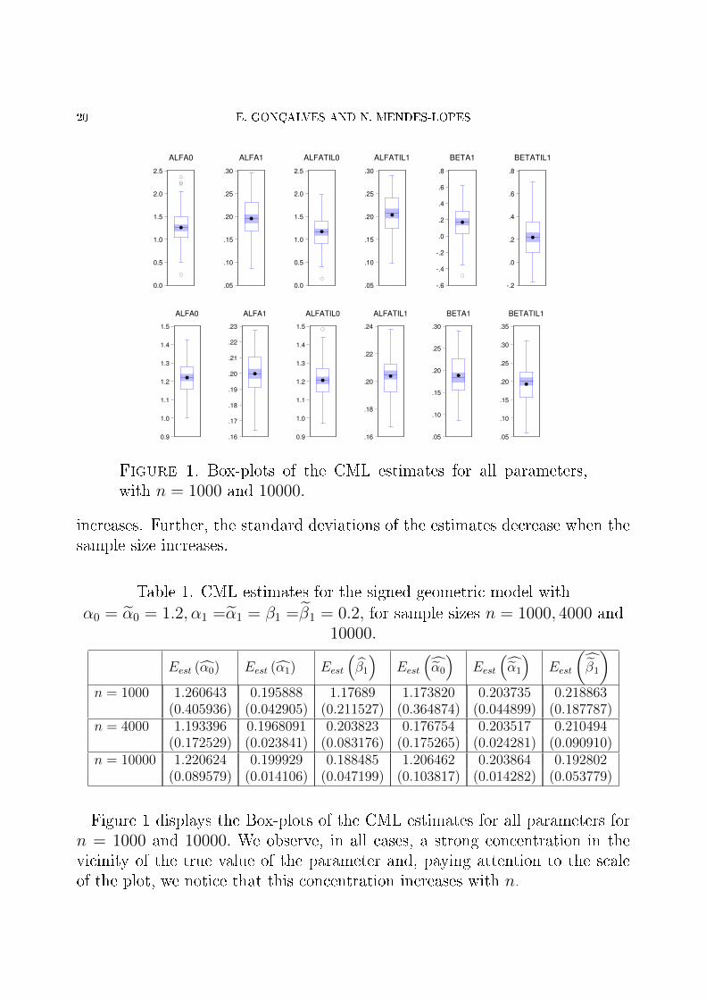
Figure 1. Box-plots of the CML estimates for all parameters,with n = 1000 and 10000.

increases. Further, the standard deviations of the estimates decrease when thesample size increases.

Table 1. CML estimates for the signed geometric model withα0 = α0 = 1.2, α1 =α1 = β1 =β1 = 0.2, for sample sizes n = 1000, 4000 and

10000.

Eest (α0) Eest (α1) Eest

(β1

)Eest

(α0

)Eest

(α1

)Eest

(β1

)n = 1000 1.260643 0.195888 1.17689 1.173820 0.203735 0.218863

(0.405936) (0.042905) (0.211527) (0.364874) (0.044899) (0.187787)n = 4000 1.193396 0.1968091 0.203823 0.176754 0.203517 0.210494

(0.172529) (0.023841) (0.083176) (0.175265) (0.024281) (0.090910)n = 10000 1.220624 0.199929 0.188485 1.206462 0.203864 0.192802

(0.089579) (0.014106) (0.047199) (0.103817) (0.014282) (0.053779)

Figure 1 displays the Box-plots of the CML estimates for all parameters forn = 1000 and 10000. We observe, in all cases, a strong concentration in thevicinity of the true value of the parameter and, paying attention to the scaleof the plot, we notice that this concentration increases with n.


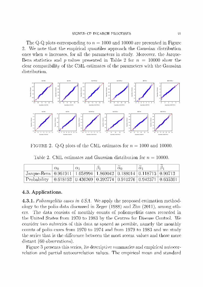
The Q-Q plots corresponding to n = 1000 and 10000 are presented in Figure2. We note that the empirical quantiles approach the Gaussian distributionones when n increases, for all the parameters in study. Moreover, the Jarque-Bera statistics and p-values presented in Table 2 for n = 10000 show theclear compatibility of the CML estimates of the parameters with the Gaussiandistribution.

0.0

0.5

1.0

1.5

2.0

2.5

0.0 0.5 1.0 1.5 2.0 2.5

Quantiles of ALFA0

Quantile

s o

f N

orm

al

ALFA0

.08

.12

.16

.20

.24

.28

.32

.05 .10 .15 .20 .25 .30

Quantiles of ALFA1

Quantile

s o

f N

orm

al

ALFA1

0.0

0.5

1.0

1.5

2.0

2.5

0.0 0.5 1.0 1.5 2.0 2.5

Quantiles of ALFATIL0

Quantile

s o

f N

orm

al

ALFATIL0

.05

.10

.15

.20

.25

.30

.35

.05 .10 .15 .20 .25 .30

Quantiles of ALFATIL1Q

uantile

s o

f N

orm

al

ALFATIL1

-.4

-.2

.0

.2

.4

.6

.8

-.6 -.4 -.2 .0 .2 .4 .6 .8

Quantiles of BETA1

Quantile

s o

f N

orm

al

BETA1

-.4

-.2

.0

.2

.4

.6

.8

-.2 .0 .2 .4 .6 .8

Quantiles of BETATIL1

Quantile

s o

f N

orm

al

BETATIL1

0.9

1.0

1.1

1.2

1.3

1.4

1.5

0.9 1.0 1.1 1.2 1.3 1.4 1.5

Quantiles of ALFA0

Quantile

s o

f N

orm

al

ALFA0

.16

.18

.20

.22

.24

.16 .17 .18 .19 .20 .21 .22 .23

Quantiles of ALFA1

Quantile

s o

f N

orm

al

ALFA1

0.9

1.0

1.1

1.2

1.3

1.4

1.5

0.9 1.0 1.1 1.2 1.3 1.4 1.5


Quantile

s o

f N

orm

al

ALFATIL0

.16

.18

.20

.22

.24

.26

.16 .18 .20 .22 .24


Quantile

s o

f N

orm

al

ALFATIL1

.05

.10

.15

.20

.25

.30

.35

.05 .10 .15 .20 .25 .30

Quantiles of BETA1

Quantile

s o

f N

orm

al

BETA1

.05

.10

.15

.20

.25

.30

.35

.05 .10 .15 .20 .25 .30 .35

Quantiles of BETATIL1

Quantile

s o

f N

orm

al

BETATIL1

Figure 2. Q-Q plots of the CML estimates for n = 1000 and 10000.

Table 2. CML estimates and Gaussian distribution for n = 10000.

α0 α1 β1 α0 α1 β1

Jarque-Bera 0.961911 1.658994 1.869042 0.188014 0.118713 0.90713Probability 0.618193 0.436269 0.392774 0.910276 0.942371 0.635361

4.3. Applications.

4.3.1.Poliomyelitis cases in USA. We apply the proposed estimation method-ology to the polio data discussed in Zeger (1988) and Zhu (2011), among oth-ers. The data consists of monthly counts of poliomyelitis cases recorded inthe United States from 1970 to 1983 by the Centres for Disease Control. Weconsider two subseries of this data as spaced as possible, namely the monthlycounts of polio cases from 1970 to 1974 and from 1979 to 1983 and we studythe series that is the di�erence between the most recent values and those moredistant (60 observations).Figure 3 presents this series, its descriptive summaries and empirical autocor-

relation and partial autocorrelation values. The empirical mean and standard


-16

-12

-8

-4

0

4

8

5 10 15 20 25 30 35 40 45 50 55 60

DIF

0

4

8

12

16

20

-12 -10 -8 -6 -4 -2 0 2 4 6

Series: DIF

Sample 1 60

Observations 60

Mean -0.450000

Median 0.000000

Maximum 6.000000

Minimum -12.00000

Std. Dev. 2.466212

Skewness -1.715012

Kurtosis 10.23537

Jarque-Bera 160.2892

Probability 0.000000

Figure 3. Di�erence series: plot, descriptive summaries and au-tocorrelation and partial autocorrelation values.

deviation of the data are −0.45 and 2.466 respectively. We conclude that therewas, on average, progress in that 10-year interval in the direction of polio eradi-cation in United States. The data is overdispersed, the autocorrelation of orderone is 0.223 and the autocorrelations of higher order are not signi�cant, whichallows inferring an order 1 dependence although not very strong.In order to model the data we consider a signed geometric INARCH model

with p = p = 1 with parameters α0, α1, α0, α1. The conditional maximumlikelihood estimates from this �tting are summarised in Table 3 (0.509345,0.293369, 0.519798 and 0.522338, respectively) leading to an estimated modelthat is �rst order stationary.The �tted conditional mean is given in Figure 4 and we note that it closely

follows the values and trend of the observed series. The resulting Pearsonresidual is de�ned by


-16

-12

-8

-4

0

4

8

5 10 15 20 25 30 35 40 45 50 55 60

CDIF COND_MEAN_EST

Figure 4. Di�erence series and �tted conditional mean from thesigned geometric INGARCH model.

rt =

Xt −(Mt −

Mt

)√Mt

(1 + Mt

)+Mt

(1 +

Mt

)where Mt = α0 + α1X1,t−1 and

Mt = α0 + α1X2,t−1. The residual analysis

is shown in Figure 5 and there is no evidence of any correlation within theresiduals. The Jarque-Bera statistics implies the normality of the Pearsonresiduals at the 0.01 signi�cance level and this fact is also suggested by thekernel density estimation and normal Q-Q plots for the Pearson residuals.

Table 3. Signed geometric INARCH model parameter estimation

4.3.2. Olympic Medals won by Swiss and Dutch athletes. Our second appli-cation consists of the number of Olympic medals won by Switzerland (S) andNetherlands (N) as displayed in https://demos.telerik.com/ aspnet-ajax/sample-applications/olympic-games/.


0

2

4

6

8

10

12

-3 -2 -1 0 1 2

Series: RPEARSON

Sample 1 60

Observations 59

Mean 0.011028

Median 0.126622

Maximum 2.280471

Minimum -2.877725

Std. Dev. 0.970987

Skewness -0.772077

Kurtosis 4.148276



.0

.1

.2

.3

.4

.5

.6

-4 -3 -2 -1 0 1 2 3 4

De

nsity

RPEARSON

-3

-2

-1

0

1

2

3

-3 -2 -1 0 1 2 3

Quantiles of RPEARSON

Qu

an

tile

s o

f N

orm

al

Figure 5. Pearson residuals: descriptive summaries, autocorrela-tion and partial autocorrelation values, kernel density estimationand Gaussian Q-Q plot.

Figure 6 presents the plot of the S-N di�erence series, its descriptive sum-maries and the empirical autocorrelation and partial autocorrelation values.The empirical mean and variance are −1.935 and 76.74, respectively. A betterperformance, on average, of Dutch athlets is observed. The data is overdis-persed and the autocorrelations of order greater than two are not signi�cant.The conditional maximum likelihood estimates after �tting a signed geo-

metric INARCH model with parameters α0, α1, α0, α2 are 1.64603, 0.306622,2.145151 and 0.476046, respectively (Table 4).

Table 4. Signed geometric INARCH model parameter α0, α1, α0, α2 estimation


-20

-10

0

10

20

30

00 08 16 24 32 40 48 56 64 72 80 88 96 04 12

DIF

0

2

4

6

8

10

12

-20 -15 -10 -5 0 5 10 15 20 25

Series: DIF

Sample 1896 2016

Observations 31

Mean -1.935484

Median -1.000000

Maximum 24.00000

Minimum -17.00000

Std. Dev. 8.759511

Skewness 0.539363

Kurtosis 4.163419



Figure 6. Di�erence series: plot, descriptive summaries and au-tocorrelation and partial autocorrelation values.

Despite the signi�cance of all the estimated parameters we decided, in viewof the small signi�cance of the order 2 autocorrelation, to �t the series by aa signed geometric INARCH model with parameters α0, α1, α0, α1. The corre-sponding estimates are now 1.374252, 0.368949, 0.81656 and 0.622359, respec-tively (Table 5). The values of the Akaike and Schwarz criteria lead us to retainthis second modeling.

Table 5. Signed geometric INARCH model parameter α0, α1, α0, α1 estimation


-20

-10

0

10

20

30

00 08 16 24 32 40 48 56 64 72 80 88 96 04 12

CDIF COND_MEAN_EST

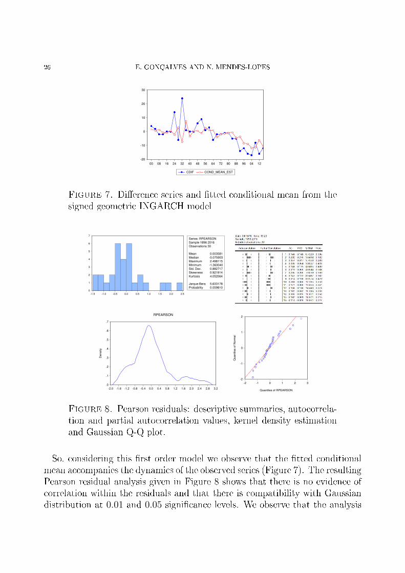
Figure 7. Di�erence series and �tted conditional mean from thesigned geometric INGARCH model

0

1

2

3

4

5

6

7

-1.5 -1.0 -0.5 0.0 0.5 1.0 1.5 2.0 2.5

Series: RPEARSON

Sample 1896 2016

Observations 30

Mean 0.003581

Median -0.075903

Maximum 2.498115

Minimum -1.363040

Std. Dev. 0.882717

Skewness 0.921914

Kurtosis 4.052064



.0

.1

.2

.3

.4

.5

.6

.7

-2.0 -1.6 -1.2 -0.8 -0.4 0.0 0.4 0.8 1.2 1.6 2.0 2.4 2.8 3.2

De

nsity

RPEARSON

-2

-1

0

1

2

-2 -1 0 1 2 3

Quantiles of RPEARSON

Qu

an

tile

s o

f N

orm

al

Figure 8. Pearson residuals: descriptive summaries, autocorrela-tion and partial autocorrelation values, kernel density estimationand Gaussian Q-Q plot.

So, considering this �rst order model we observe that the �tted conditionalmean accompanies the dynamics of the observed series (Figure 7). The resultingPearson residual analysis given in Figure 8 shows that there is no evidence ofcorrelation within the residuals and that there is compatibility with Gaussiandistribution at 0.01 and 0.05 signi�cance levels. We observe that the analysis


of the Pearson residuals for the second order model, �rstly considered, led toworst results con�rming the decision based on the criteria.

5. Conclusion

Time series of counts appear in a large variety of contexts like in studies ofthe incidence of a certain disease in a country, number of daily transactions ona �nancial market or number of accidents in a town. This kind of time seriesoften reveals overdispersion and conditional heteroscedasticity and the largefamily of integer-valued CP-INGARCH models has wide potential to describeand capture these characteristics.With the aim of modeling the di�erence of two count time series, we propose

in this paper a bivariate model de�ned by two independent CP-INGARCHprocesses. A Z-valued counting process is then de�ned as the di�erence betweenthe two marginal processes. The signed integer-valued process de�ned by theSkellam distribution, which is constructed as di�erences in pairs of Poissoncounts, is included in this study if the counts series are independent.Since the Poissonian models are not the most adequated to model overdis-

persed series we concentrated our study in the geometric models, a particularcase of the NB-INARCH ones. The probabilistic and statistical study here de-veloped shows that this family of Z-valued models may be useful in applicationswhere the analysis of the di�erence of count time series is relevant.Although we have privileged the di�erence of the two marginal processes,

we note that any other measurable function of these processes may be consid-ered and emphasize that the main probabilistic properties of such models havealready been here stated.

Acknowledgements

This work was partially supported by the Centre for Mathematics of the Uni-versity of Coimbra - UID/MAT/00324/2013 funded by the Portuguese Govern-ment trough FCT/MEC and co-funded by the European Regional DevelopmentFund through the Partnership Agreement PT2020.

References[1] Abramowitz M, Stegun I (eds.). 1965. Handbook of Mathematical Functions, New York: Dover

Publications, Inc.[2] Durrett R. 2010. Probability: Theory and Examples, Cambridge University Press (4th edn).[3] Ferland R, Latour A, Oraichi D. 2006. Integer-valued GARCH process., J. Time Ser. Analysis,

27, 923�42.


[4] Fokianos K, Rahbek A, Tjøtheim D. 2009. Poisson autoregression, Journal of the AmericanStatistical Association, 104, 1430�39.

[5] Gonçalves E, Mendes-Lopes N, Silva F. 2015. In�nitely divisible distributions in integer-valued

GARCH models, J. Time Ser. Analysis, 36, 503-527.[6] Gonçalves E, Mendes-Lopes N, Silva F. 2016. Zero-in�ated compound Poisson distributions in

integer-valued GARCH models, Statistics, 50, 558-578.[7] Halmos P. 1974. Measure Theory, New York: Springer-Verlag.[8] Karlis D, Ntzoufras I. 2006. Bayesian analysis of the di�erences of count data, Statistics in

Medicine, 25, 1885�1905.[9] Karlis D, Ntzoufras I. 2009. Bayesian modelling of football outcomes: using the Skellam distri-

bution for the goal di�erence, IMAJ of Management Mathematics, 20, 133�145.[10] Kim HY, Park Y. 2008. A non-stationary integer-valued autoregressive model, Statistical Pa-

pers, 49, 485�502.[11] Koopman SJ, Lit R, Lucas A. 2014. The Dynamic Skellam Model with Applica-

tions, Tinbergen Institute Discussion Paper 14-032/IV/DSF73, Available at SSRN:https://ssrn.com/abstract=2406867 or http://dx.doi.org/10.2139/ssrn.2406867.

[12] Scotto MG, Weiÿ CH, Gouveia S. 2015.Thinning-based models in the analysis of integer-valued

time series: A review, Statistical Modelling, 15(6): 590�618.[13] Skellam JG. 1946.The frequency distribution of the di�erence between two Poisson variates

belonging to di�erent populations, J. of the Royal Statistical Society, A, 109 (3), 296-.[14] Weiÿ CH. 2009. Modelling time series of counts with overdispersion, Statistical Methods and

Applications, 18, 507�519.[15] Xu H-Y, Xie M, Goh TN., Fu X. 2012. A model for integer-valued time series with conditional

overdispersion,Computational Statistics and Data Analysis, 56, 4229�4242.[16] Zeger SL. 1988.A regression model for time series of counts, Biometrika, 75, 621-629.[17] Zhu F. 2011. A negative binomial integer-valued GARCH model, J. Time Ser. Anal. 32, 54�67.[18] Zhu F. 2012. Modelling overdispersed or underdispersed count data with generalized Poisson

integer-valued GARCH models,Journal of Mathematical Analysis and Applications, 389 1, 58�71.

[19] Zhu F, Li Q, Wang D. 2010.A mixture integer-valued ARCH model, Journal of Stat. Plann.and Inf., 140, 2025�2036.

E. Gonçalves

CMUC, Department of Mathematics, University of Coimbra, 3001-501 Coimbra, Portugal

E-mail address: [email protected]

N. Mendes-Lopes

CMUC, Department of Mathematics, University of Coimbra, 3001-501 Coimbra, Portugal

E-mail address: [email protected]

integer-valued garch processes - mat.uc.pt · duced in gonçalves et al (2015), that enlarges and...

Documents