integer programming - guilanstaff.guilan.ac.ir/staff/users/salahi/fckeditor_repo/... · ·...

Sven O. Krumke

Integer ProgrammingPolyhedra and Algorithms

Draft: January 4, 2006

0 1 2 3 4 5

0

1

2

3

4

5 S

G

shrink S

shrink S = V \ S

GS

S

GS

S

V \ S

ii

These course notes are based on my lectures»Integer Programming: Polyhedral Theory«and »Integer Programming: Algorithms« atthe University of Kaiserslautern.

I would be happy to receive feedback, inparticular suggestions for improvement andnotificiations of typos and other errors.

Sven O. Krumkekrumkemathematik.uni-kl.de

Contents

1 Introduction 1

1.1 Integer Linear Programs . . . . . . . . . . . . . . . . . . . . . . . . . . . . . . . . . . 1

1.2 Notes of Caution . . . . . . . . . . . . . . . . . . . . . . . . . . . . . . . . . . . . . . 4

1.3 Examples . . . . . . . . . . . . . . . . . . . . . . . . . . . . . . . . . . . . . . . . . . . 5

1.4 Literature . . . . . . . . . . . . . . . . . . . . . . . . . . . . . . . . . . . . . . . . . . . 10

1.5 Acknowledgements . . . . . . . . . . . . . . . . . . . . . . . . . . . . . . . . . . . . . 10

2 Basics 11

2.1 Notation . . . . . . . . . . . . . . . . . . . . . . . . . . . . . . . . . . . . . . . . . . . 11

2.2 Convex Hulls . . . . . . . . . . . . . . . . . . . . . . . . . . . . . . . . . . . . . . . . 11

2.3 Polyhedra and Formulations . . . . . . . . . . . . . . . . . . . . . . . . . . . . . . . 13

2.4 Linear Programming . . . . . . . . . . . . . . . . . . . . . . . . . . . . . . . . . . . . 15

2.5 Agenda . . . . . . . . . . . . . . . . . . . . . . . . . . . . . . . . . . . . . . . . . . . . 16

I Polyhedral Theory 17

3 Polyhedra and Integer Programs 19

3.1 Valid Inequalities and Faces of Polyhedra . . . . . . . . . . . . . . . . . . . . . . . . 19

3.2 Dimension . . . . . . . . . . . . . . . . . . . . . . . . . . . . . . . . . . . . . . . . . . 22

3.3 Extreme Points . . . . . . . . . . . . . . . . . . . . . . . . . . . . . . . . . . . . . . . . 29

3.4 Facets . . . . . . . . . . . . . . . . . . . . . . . . . . . . . . . . . . . . . . . . . . . . . 34

3.5 Minkowski’s Theorem . . . . . . . . . . . . . . . . . . . . . . . . . . . . . . . . . . . 38

3.6 Most IPs are Linear Programs . . . . . . . . . . . . . . . . . . . . . . . . . . . . . . . 42

4 Integrality of Polyhedra 47

4.1 Equivalent Definitions of Integrality . . . . . . . . . . . . . . . . . . . . . . . . . . . 48

4.2 Matchings and Integral Polyhedra I . . . . . . . . . . . . . . . . . . . . . . . . . . . 49

4.3 Total Unimodularity . . . . . . . . . . . . . . . . . . . . . . . . . . . . . . . . . . . . 50

4.4 Conditions for Total Unimodularity . . . . . . . . . . . . . . . . . . . . . . . . . . . 52

4.5 Applications of Unimodularity: Network Flows . . . . . . . . . . . . . . . . . . . . 54

4.6 Matchings and Integral Polyhedra II . . . . . . . . . . . . . . . . . . . . . . . . . . . 57

4.7 Total Dual Integrality . . . . . . . . . . . . . . . . . . . . . . . . . . . . . . . . . . . . 61

4.8 Submodularity and Matroids . . . . . . . . . . . . . . . . . . . . . . . . . . . . . . . 64

iv

II Algorithms 69

5 Basics about Problems and Complexity 715.1 Encoding Schemes, Problems and Instances . . . . . . . . . . . . . . . . . . . . . . . 715.2 The Classes P and NP . . . . . . . . . . . . . . . . . . . . . . . . . . . . . . . . . . . . 735.3 The Complexity of Integer Programming . . . . . . . . . . . . . . . . . . . . . . . . 765.4 Optimization and Separation . . . . . . . . . . . . . . . . . . . . . . . . . . . . . . . 77

6 Relaxations and Bounds 816.1 Optimality and Relaxations . . . . . . . . . . . . . . . . . . . . . . . . . . . . . . . . 816.2 Combinatorial Relaxations . . . . . . . . . . . . . . . . . . . . . . . . . . . . . . . . . 846.3 Lagrangian Relaxation . . . . . . . . . . . . . . . . . . . . . . . . . . . . . . . . . . . 886.4 Duality . . . . . . . . . . . . . . . . . . . . . . . . . . . . . . . . . . . . . . . . . . . . 94

7 Dynamic Programming 977.1 Shortest Paths Revisited . . . . . . . . . . . . . . . . . . . . . . . . . . . . . . . . . . 977.2 Knapsack Problems . . . . . . . . . . . . . . . . . . . . . . . . . . . . . . . . . . . . . 997.3 Problems on Trees . . . . . . . . . . . . . . . . . . . . . . . . . . . . . . . . . . . . . . 101

8 Branch and Bound 1038.1 Divide and Conquer . . . . . . . . . . . . . . . . . . . . . . . . . . . . . . . . . . . . 1038.2 Pruning Enumeration Trees . . . . . . . . . . . . . . . . . . . . . . . . . . . . . . . . 1038.3 LP-Based Branch and Bound: An Example . . . . . . . . . . . . . . . . . . . . . . . 1068.4 Techniques for LP-based Branch and Bound . . . . . . . . . . . . . . . . . . . . . . . 109

9 Cutting Planes 1159.1 Cutting-Plane Proofs . . . . . . . . . . . . . . . . . . . . . . . . . . . . . . . . . . . . 1159.2 A Geometric Approach to Cutting Planes: The ChvÃ¡tal Rank . . . . . . . . . . . . 1219.3 Cutting-Plane Algorithms . . . . . . . . . . . . . . . . . . . . . . . . . . . . . . . . . 1239.4 Gomory’s Cutting-Plane Algorithm . . . . . . . . . . . . . . . . . . . . . . . . . . . 1259.5 Mixed Integer Cuts . . . . . . . . . . . . . . . . . . . . . . . . . . . . . . . . . . . . . 1319.6 Structured Inequalities . . . . . . . . . . . . . . . . . . . . . . . . . . . . . . . . . . . 133

10 Column Generation 14510.1 Dantzig-Wolfe Decomposition . . . . . . . . . . . . . . . . . . . . . . . . . . . . . . . 14510.2 Dantzig-Wolfe Reformulation of Integer Programs . . . . . . . . . . . . . . . . . . . 148

11 More About Lagrangean Duality 15711.1 Convexity and Subgradient Optimization . . . . . . . . . . . . . . . . . . . . . . . . 15711.2 Subgradient Optimization for the Lagrangean Dual . . . . . . . . . . . . . . . . . . 16011.3 Lagrangean Heuristics and Variable Fixing . . . . . . . . . . . . . . . . . . . . . . . 162

A Notation 165A.1 Basics . . . . . . . . . . . . . . . . . . . . . . . . . . . . . . . . . . . . . . . . . . . . . 165A.2 Sets and Multisets . . . . . . . . . . . . . . . . . . . . . . . . . . . . . . . . . . . . . . 165A.3 Analysis and Linear Algebra . . . . . . . . . . . . . . . . . . . . . . . . . . . . . . . . 166A.4 Growth of Functions . . . . . . . . . . . . . . . . . . . . . . . . . . . . . . . . . . . . 166A.5 Particular Functions . . . . . . . . . . . . . . . . . . . . . . . . . . . . . . . . . . . . 166A.6 Probability Theory . . . . . . . . . . . . . . . . . . . . . . . . . . . . . . . . . . . . . 167A.7 Graph Theory . . . . . . . . . . . . . . . . . . . . . . . . . . . . . . . . . . . . . . . . 167A.8 Theory of Computation . . . . . . . . . . . . . . . . . . . . . . . . . . . . . . . . . . 169

v

B Symbols 171

Bibliography 173

Introduction

Linear Programs can be used to model a large number of problems arising inpractice. A standard form of a Linear Program is

(LP) max cT x(1.1a)

Ax ≤ b(1.1b)

x ≥ 0,(1.1c)

where c ∈ Rn, b ∈ Rm are given vectors and A ∈ Rm×n is a matrix. The focusof these lecture notes is to study extensions of Linear Programs where we aregiven additional integrality conditions on all or some of the variables.

Problems with integrality constraints on the variables arise in a variety of ap-plications. For instance, if we want to place facilities, it makes sense to requirethe number of facilites to be an integer (it is not clear what it means to build2.28 fire stations). Also, frequently, one can model decisions as 0-1-variables:the variable is zero if we make a negative decision and one otherwise.

1.1 Integer Linear Programs

We first state the general form of a Mixed Integer Program as it will be usedthroughout these notes:

Definition 1.1 (Mixed Integer Linear Program (MIP))A Mixed Integer Linear Program (MIP) is given by vectors c ∈ Rn, b ∈ Rm, amatrix A ∈ Rm×n and a number p ∈ 0, . . . , n. The goal of the problem is to find avector x ∈ Rn solving the following optimization problem:

(MIP) max cT x(1.2a)

Ax ≤ b(1.2b)

x ≥ 0(1.2c)

x ∈ Zp × Rn−p.(1.2d)

If p = 0, then then there are no integrality constraints at all, so we obtain the LinearProgram (1.1). On the other hand, if p = n, then all variables are required to beintegral. In this case, we speak of an Integer Linear Program (IP): we note again forlater reference:

(IP) max cT x(1.3a)

Ax ≤ b(1.3b)

x ≥ 0(1.3c)

x ∈ Zn(1.3d)

2 Introduction

If in an (IP) all variables are restricted to values from the set B = 0, 1, we have a0-1-Integer Linear Program or Binary Linear Integer Program:

(BIP) max cT x(1.4a)

Ax ≤ b(1.4b)

x ≥ 0(1.4c)

x ∈ Bn(1.4d)

Most of the time we will be concerned with Integer Programs (IP) and BinaryInteger Programs (BIP).

Example 1.2Consider the following Integer Linear Program:

max x + y(1.5a)

2y − 3x ≤ 2(1.5b)

x + y ≤ 5(1.5c)

1 ≤ x ≤ 3(1.5d)

1 ≤ y ≤ 3(1.5e)

x, y ∈ Z(1.5f)

The feasible region S of the problem is depicted in Figure 1.1. It consists of theintegral points emphasized in red, namely

S = (1, 1), (2, 1), (3, 1), (1, 2), (2, 2), (3, 2), (2, 3).

0 1 2 3 4 5

0

1

2

3

4

5

b b b

b b b

b

Figure 1.1: Example of the feasible region of an integer program.

⊳

Example 1.3 (Knapsack Problem)A climber is preparing for an expedition to Mount Optimization. His equip-ment consists of n items, where each item i has a profit pi ∈ Z+ and aweight wi ∈ Z+. The climber knows that he will be able to carry items of

1.2 Notes of Caution 3

total weight at most b ∈ Z+. He would like to pack his knapsack in such away that he gets the largest possible profit without exceeding the weight limit.

We can formulate the KNAPSACK problem as a (BIP). Define a decision vari-able xi, i = 1, . . . , n with the following meaning:

xi =

1 if item i gets packed into the knapsack0 otherwise

Then, KNAPSACK becomes the (BIP)

maxn∑

i=1

pixi(1.6a)

n∑

i=1

wixi ≤ b(1.6b)

x ∈ Bn(1.6c)

⊳

In the preceeding example we have essentially identified a subset of the pos-sible items with a 0-1-vector. Given a ground set E, we can associate with eachsubset F ⊆ E an incidence vector χF ∈ RF by setting

χFe =

1 if e ∈ F

0 if e /∈ F.

Then, we can identify the vector χF with the set F and vice versa. We will seenumerous examples of this identification in the rest of these lecture notes. Thisidentification appears frequently in the context of combinatorial optimizationproblems.

Definition 1.4 (Combinatorial Optimization Problem)A combinatorial optimization problem is given by a finite ground set N, a weightfunction c : N→ R and a family F ⊆ 2N of feasible subsets of N. The goal is to solve

(1.7) (COP) min

∑

j∈S

cj : S ∈ F

.

Thus, we can write KNAPSACK also as (COP) by using:

N := 1, . . . , n

F :=

S ⊆ N :∑

i∈S

wi ≤ b

,

and c(i) := −wi. We will see later that there is a close connection betweencombinatorial optimization problems (as stated in (1.7)) and Integer LinearPrograms.

4 Introduction

0 1 2 3 4 5 6 7 8

0

1

2

3

4

5

6

7

8

y =√

2xx = 1

y = 0

Figure 1.2: An IP without optimal solution.

1.2 Notes of Caution

Integer Linear Programs are qualitatively different from Linear Programs in anumber of aspects. Recall that from the Fundamental Theorem of Linear Pro-gramming we know that, if the Linear Program (1.1) is feasible and bounded,it has an optimal solution.

Now, consider the following Integer Linear Program:

max −√

2x + y(1.8a)

−√

2x + y ≤ 0(1.8b)

x ≥ 1(1.8c)

y ≥ 0(1.8d)

x, y ∈ Z(1.8e)

The feasible region S of the IP (1.8) is depicted in Figure 1.2. The set of feasiblesolutions is nonempty (for instance (1, 0) is a feasible point) and by the con-straint −

√2x+y ≤ 0 the objective is also bounded from above on S. However,

the IP does not have an optimal solution!

To see this, observe that from the constraint −√

2x + y ≤ 0 we have y/x ≤√

2

and, since we know that√

2 is irrational, −√

2x + y < 0 for any x, y ∈ Z. Onthe other hand, for integral x, the function −

√2x+ ⌊

√2x⌋ gets arbitrarily close

to 0.

Remark 1.5 An IP with irrational input data can be feasible and bounded butmay still not have an optimal solution.

1.3 Examples 5

The reason why the IP (1.8) does not have an optimal solution lies in the factthat we have used irrational data to specify the problem. We will see later thatunder the assumption of rational data any feasible and bounded MIP musthave an optimal solution. We stress again that for standard Linear Programsno assumption about the input data is needed.

At first sight it might sound like a reasonable idea to simply drop the inte-grality constraints in an IP and to “round the corresponding” solution. But, ingeneral, this is not a good idea for the following reasons:

• The rounded solution may be infeasible (see Figure 1.3(a)), or

• the rounded solution may be feasible but far from the optimum solution(see Figure 1.3(b)).

x∗

cT x

(a)

x∗

cT x

(b)

Figure 1.3: Simply rounding a solution of the LP-relaxation to an IP may giveinfeasible or very bad solutions.

1.3 Examples

In this section we give various examples of integer programming problems.

Example 1.6 (Assignment Problem)Suppose that we are given n tasks and n people which are available for car-rying out the tasks. Each person can carry out exactly one job, and there is acost cij if person i serves job j. How should we assign the jobs to the personsin order to minimize the overall cost?

We first introduce binary decision variables xij with the following meaning:

xij =

1 if person i carrys out job j

0 otherwise.

Given such a binary vector x, the number of persons assigned to job j is ex-actly

∑n

i=1 xij. Thus, the requirement that each job gets served by exactly oneperson can be enforced by the following constraint:

n∑

i=1

xij = 1, for j = 1, . . . , n.

Similarly, we can ensure that each person does exactly one job by having thefollowing constraint:

n∑

j=1

xij = 1, for i = 1, . . . , n.

6 Introduction

We obtain the following BIP:

minn∑

i=1

n∑

j=1

cijxij

n∑

i=1

xij = 1 for j = 1, . . . , n

n∑

j=1

xij = 1 for i = 1, . . . , n

x ∈ Bn2

⊳

Example 1.7 (Uncapacitated Facility Location Problem)In the uncapacitated facility location problem (UFL) we are given a set of potentialdepots M = 1, . . . , m and a set N = 1, . . . , n of clients. Opening a depot atsite j involves a fixed cost fj. Serving client i by a depot at location j costs cij

units of money. The goal of the UFL is to decide at which positions to opendepots and how to serve all clients such as to minimize the overall cost.

We can model the cost cij which arises if client i is served by a facility at j withthe help of binary variables xij similar to the assignment problem:

xij =

1 if client i is served by a facility at j

0 otherwise.

The fixed cost fj which arises if we open a facility at j can be handled by binaryvariables yj where

yj =

1 if a facility at j is opened0 otherwise.

Following the ideas of the assignment problem, we obtain the following BIP:

minm∑

j=1

fjyj +

m∑

j=1

n∑

i=1

cijxij(1.9a)

m∑

j=1

xij = 1 for i = 1, . . . , n(1.9b)

x ∈ Bnm, y ∈ Bm(1.9c)

As in the assignment problem, constraint (1.9b) enforces that each client isserved. But our formulation is not complete yet! The current constraints allowa client i to be served by a facility at j which is not opened, that is, whereyj = 0. How can we ensure that clients are only served by open facilities?

One option is to add the nm constraints xij ≤ yj for all i, j to (1.9). Then, ifyj = 0, we must have xij = 0 for all i. This is what we want. Hence, the UFL

1.3 Examples 7

can be formulated as follows:

minm∑

j=1

fjyj +

m∑

j=1

n∑

i=1

cijxij(1.10a)

m∑

j=1

xij = 1 for i = 1, . . . , n(1.10b)

xij ≤ yj for i = 1, . . . , n and j = 1, . . . , m(1.10c)

x ∈ Bnm, y ∈ Bm(1.10d)

A potential drawback of the formulation (1.10) is that it contains a large num-ber of constraints. We can formulate the condition that clients are served onlyby open facilities in another way. Observe that

∑ni=1 xij is the number of

clients assigned to facility j. Since this number is an integer between 0 and n,the condition

∑n

i=1 xij ≤ nyj can also be used to prohibit clients being servedby a facility which is not open. If yj = 0, then

∑ni=1 xij must also be zero. If

yj = 1, we have the constraint∑n

i=1 xij ≤ n which is always satisfied sincethere is a total of n clients. This gives us the alternative formulation of theUFL:

minm∑

j=1

fjyj +

m∑

j=1

n∑

i=1

cijxij(1.11a)

m∑

j=1

xij = 1 for i = 1, . . . , n(1.11b)

n∑

i=1

xij ≤ nyj for j = 1, . . . , m(1.11c)

x ∈ Bnm, y ∈ Bm(1.11d)

Are there any differences between the two formulations as far as solvability isconcerned? We will explore this question later in greater detail. ⊳

Example 1.8 (Traveling Salesman Problem)In the traveling salesman problem (TSP) a salesman must visit each of n givencities V = 1, . . . , n exactly once and then return to his starting point. Thedistance between city i and j is cij. The salesman wants to find a tour ofminimum length.

The TSP can be modeled as a graph problem by considering a complete di-rected graph G = (V, A), that is, a graph with A = V × V , and assigning a costc(i, j) to every arc a = (i, j). A tour is then a cycle in G which touches everynode in V exactly once.

We formulate the TSP as a BIP. We have binary variables xij with the followingmeaning:

xij =

1 if the salesman goes from city i directly to city j

0 otherwise.

Then, the total length of the tour taken by the salesman is∑

i,j cijxij. In afeasible tour, the salesman enters each city exactly once and also leaves each

8 Introduction

city exactly once. Thus, we have the constraints:∑

j:j6=i

xji = 1 for i = 1, . . . , n

∑

j:j6=i

xij = 1 for i = 1, . . . , n.

However, the constraints specified so far do not ensure that a binary solutionforms indeed a tour.

2

1 4 5

3

Figure 1.4: Subtours are possible in the TSP if no additional constraints areadded.

Consider the situation depicted in Figure 1.4. We are given five cities and foreach city there is exactly one incoming and one outgoing arc. However, thesolution is not a tour but a collection of directed cycles called subtours.

To elminimate subtours we have to add more constraints. One possible way ofdoing so is to use the so-called subtour elimination constraints. The underlyingidea is as follows. Let ∅ 6= S ⊂ V be a subset of the cities. A feasible tour(on the whole set of cities) must leave S for some vertex outside of S. Hence,the number of arcs that have both endpoints in S can be at most |S| − 1. Onthe other hand, a subtour which is a directed cycle for a set ∅ 6= S ⊂ V , hasexactly |S| arcs with both endpoints in S. We obtain the following BIP for theTSP:

minn∑

i=1

n∑

j=1

cijxij(1.12a)

∑

j:j6=i

xij = 1 for i = 1, . . . , n(1.12b)

∑

i:i6=j

xij = 1 for j = 1, . . . , n(1.12c)

∑

i∈S

∑

j∈S

xij ≤ |S| − 1 for all ∅ ⊂ S ⊂ V.(1.12d)

x ∈ Bn(n−1)(1.12e)

As mentioned before, the constraints (1.12d) are called subtour elimination con-straints. ⊳

Example 1.9 (Set-Covering, Set-Packing and Set-Partitioning Problem)Let U be a finite ground set and F ⊆ 2U be a collection of subsets of U. Thereis a cost/benefit cf associated with every set f ∈ F. In the the set covering

1.3 Examples 9

(set packing, set partitioning) problem we wish to find a subcollection of thesets in F such that each element in U is covered at least once (at most once,exactly once). The goal in the set covering and set partitioning problem is tominimize the cost of the chosen sets, whereas in the set packing problem wewish to maximize the benefit.

We can formulate each of these problems as a BIP by the following approach.We choose binary variables yf, f ∈ F with the meaning that

xf =

1 if set f is chosen to be in the selection0 otherwise.

Let A = (auf) be the |U|×|F|-matrix which reflects the element-set containmentrelations, that is

auf :=

1 if element u is contained in set f

0 otherwise.

Then, the constraint that every element is covered at least once (at most once,exactly once) can be expressed by the linear constraints Ax ≥ 1 (Ax ≤ 1,Ax = 1), where 1 = (1, . . . , 1) ∈ RU is the vector consisting of all ones. ⊳

Example 1.10 (Minimum Spanning Tree Problem)A spanning tree in an undirected graph G = (V, E) is a subgraph T = (V, F)

of G which is connected and does not contain cycles. Given a cost functionc : E→ R+ on the edges of G the minimum spanning tree problem (MST-Problem)asks to find a spanning tree T of minimum weight c(F).

We choose binary indicator variables xe for the edges in E with the meaningthat xe = 1 if and only if e is included in the spanning tree. The objectivefunction

∑e∈E cexe is now clear. But how can we formulate the requirement

that the set of edges chosen forms a spanning tree?

A cut in an undirected graph G is a partition S∪ S = V , S∩ S = ∅ of the vertexset. We denote by δ(S) the set of edges in the cut, that is, the set of edges whichhave exactly one endpoint in S. It is easy to see that a subset F ⊆ E of the edgesforms a connected spanning subgraph (V, F) if and only if F ∩ δ(S) 6= ∅ for allsubsets S with ∅ ⊂ S ⊂ V . Hence, we can formulate the requirement that thesubset of edges chosen forms a connected spanning subgraph by having theconstraint

∑e∈δ(S) xe ≥ 1 for each such subset. This gives the following BIP:

min∑

e∈E

cexe(1.13a)

∑

e∈δ(S)

xe ≥ 1 for all ∅ ⊂ S ⊂ V(1.13b)

x ∈ BE(1.13c)

How do we incorporate the requirement that the edge set chosen should bewithout cycles? The answer is that we do not need to, as far as optimality isconcerned! The reason behind that is the following: if χF is a feasible solutionfor (1.13) and F contains a cycle, we can remove one edge e from the cycle andF \ e is still feasible. Since c is nonnegative, the vector χF\e is a feasiblesolution for (1.13) of cost at most that of χF. ⊳

10 Introduction

1.4 Literature

These notes are a revised version of [Kru04], which followed more closelythe book by Laurence Wolsey [Wol98]. Classical books about Linear andInteger Programming are the books of George Nemhauser and LaurenceWolsey [NW99] and Alexander Schrijver [Sch86]. You can also find a lotof useful stuff in the books [CC+98, Sch03, GLS88] which are mainly aboutcombinatorial optimization. Section 5.3 discusses issues of complexity. Aclassical book about the theory of computation is the book by Garey andJohnson [GJ79]. More books from this area are [Pap94, BDG88, BDG90].

1.5 Acknowledgements

I wish to thank all students of the lecture »Optimization II: Integer Program-ming« at the Technical University of Kaiserslautern (winter semester 2003/04)for their comments and questions. Particular thanks go to all students whoactively reported typos and provided constructive criticism: Robert Dorbritz,Ulrich Dürholz, Tatjana Kowalew, Erika Lind, Wiredu Sampson and PhillipSüß. Needless to say, all remaining errors and typos are solely my faults!

Basics

In this chapter we introduce some of the basic concepts that will be useful forthe study of integer programming problems.

2.1 Notation

Let A ∈ Rm×n be a matrix with row index set M = 1, . . . , m and columnindex set N = 1, . . . , n. We write

A = (aij)i=1,...,mj=1,...,n

A·,j =

a1j

...amj

: jth column of A

Ai,· = (ai1, . . . , an1) : ith row of A.

For subsets I ⊆ M and J ⊆ N we denote by

AI,J := (aij)i∈Ij∈J

the submatrix of A formed by the corresponding indices. We also set

A·,J := AM,J

AI,· := AI,N.

For a subset X ⊆ Rn we denote by

lin(X) := x =

k∑

i=1

λivi : λi ∈ R and v1, . . . , vk ∈ X

the linear hull of X.

2.2 Convex Hulls

Definition 2.1 (Convex Hull)Given a set X ⊆ Rn, the convex hull of X, denoted by conv(X) is defined to be theset of all convex combinations of vectors from X, that is,

conv(X) := x =

k∑

i=1

λivi : λi ≥ 0,

k∑

i=1

λi = 1 and v1, . . . , vk ∈ X

12 Basics

Suppose that X ⊆ Rn is some set, for instance X is the set of incidence vectorsof all spanning trees of a given graph (cf. Example 1.10). Suppose that we wishto find a vector x ∈ X maximizing cTx.

If x =∑k

i=1 λivi ∈ conv(X) is a convex combination of the vectors v1, . . . , vk,then

cT x =

k∑

i=1

λicT vi ≤ maxcTvi : i = 1, . . . , k.

Hence, we have that

max cT x : x ∈ X = max cTx : x ∈ conv(X)

for any set X ⊆ Rn.

Observation 2.2 Let X ⊆ Rn be any set and c ∈ Rn be any vector. Then

(2.1) max cTx : x ∈ X = max cTx : x ∈ conv(X) .

Proof: See above. 2

Observation 2.2 may seem of little use, since we have replaced a discrete finiteproblem (left hand side of (2.1) by a continuous one (right hand side of (2.1)).However, in many cases conv(X) has a nice structure that we can exploit inorder to solve the problem. It turns out that “most of the time” conv(X) is apolyhedron x : Ax ≤ b (see Section 2.3) and that the problem max cTx : x ∈conv(X) is a Linear Program.

Example 2.3We return to the IP given in Example 1.2:

max x + y

2y − 3x ≤ 2

x + y ≤ 5

1 ≤ x ≤ 3

1 ≤ y ≤ 3

x, y ∈ Z

We have already noted that the set X of feasible solutions for the IP is

X = (1, 1), (2, 1), (3, 1), (1, 2), (2, 2), (3, 2), (2, 3).

Observe that the constraint y ≤ 3 is actually superfluous, but that is not ourmain concern right now. What is more important is the fact that we obtain thesame feasible set if we add the constraint x − y ≥ −1 as shown in Figure 2.1.Moreover, we have that the convex hull conv(X) of all feasible solutions forthe IP is described by the following inequalities:

2y − 3x ≤ 2

x + y ≤ 5

−x + y ≤ 1

1 ≤ x ≤ 3

1 ≤ y ≤ 3

2.3 Polyhedra and Formulations 13

0 1 2 3 4 5

0

1

2

3

4

5

b b b

b b b

b

Figure 2.1: The addition of a the new constraint x − y ≥ −1 (shown as the redline) leads to the same set feasible set.

Observation 2.2 now implies that instead of solving the original IP we can alsosolve the Linear Program

max x + y

2y − 3x ≤ 2

x + y ≤ 5

−x + y ≤ 1

1 ≤ x ≤ 3

1 ≤ y ≤ 3

that is, a standard Linear Program without integrality constraints. ⊳

In the above example we reduced the solution of an IP to solving a standardLinear Program. We will see later that in principle this reduction is alwayspossible (provided the data of the IP is rational). However, there is a catch!The mentioned reduction might lead to an exponential increase in the problemsize. Sometimes we might still overcome this problem (see Section 5.4).

2.3 Polyhedra and Formulations

Definition 2.4 (Polyhedron, polytope)A polyhedron is a subset of Rn described by a finite set of linear inequalities, that is,a polyhedron is of the form

(2.2) P(A, b) := x ∈ Rn : Ax ≤ b ,

where A is an m×n-matrix and b ∈ Rm is a vector. The polyhedron P is a rationalpolyhedron if A and b can be chosen to be rational. A bounded polyhedron is calledpolytope.

In Section 1.3 we have seen a number of examples of Integer Linear Programsand we have spoken rather informally of a formulation of a problem. We nowformalize the term formulation:

14 Basics

Definition 2.5 (Formulation)A polyhedron P ⊆ Rn is a formulation for a set X ⊆ Zp ×Rn−p, if X = P ∩ (Zp ×Rn−p).

It is clear, that in general there is an infinite number of formulations for a set X.This naturally raises the question about “good” and “not so good” formula-tions.

We start with an easy example which provides the intuition how to judge for-mulations. Consider again the set X = (1, 1), (2, 1), (3, 1), (1, 2), (2, 2), (3, 2), (2, 3) ⊂R2 from Examples 1.2 and 2.3. Figure 2.2 shows our known two formula-tions P1 and P2 together with a third one P3.

P1 =

(

x

y

)

:

2y − 3x ≤ 2

x + y ≤ 5

1 ≤ x ≤ 3

1 ≤ y ≤ 3

P2 =

(

x

y

)

:

2y − 3x ≤ 2

x + y ≤ 5

−x + y ≤ 1

1 ≤ x ≤ 3

1 ≤ y ≤ 3

0 1 2 3 4 5

0

1

2

3

4

5

b b b

b b b

b

Figure 2.2: Different formulations for the integral set X =

(1, 1), (2, 1), (3, 1), (1, 2), (2, 2), (3, 2), (2, 3)

Intuitively, we would rate P2 much higher than P1 or P3. In fact, P2 is anideal formulation since, as we have seen in Example 2.3 we can simply solve aLinear Program over P2, the optimal solution will be an extreme point whichis a point from X.

Definition 2.6 (Better and ideal formulations)Given a set X ⊆ Rn and two formulations P1 and P2 for X, we say that P1 is betterthan P2, if P1 ⊂ P2.

A formulation P for X is called ideal, if P = conv(X).

We will see later that the above definition is one of the keys to solving IPs.

2.4 Linear Programming 15

Example 2.7In Example 1.7 we have seen two possibilities to formulate the UncapacitatedFacility Location Problem (UFL):

minn∑

j=1

fjyj +

m∑

j=1

n∑

i=1

cijxij minn∑

j=1

fjyj +

m∑

j=1

n∑

i=1

cijxij

x ∈ P1 x ∈ P2

x ∈ Bnm, y ∈ Bm x ∈ Bnm, y ∈ Bm,

where

P1 =

(x

y

)

:

∑m

j=1 xij = 1 for i = 1, . . . , n

xij ≤ yj for i = 1, . . . , n and j = 1, . . . , m

P2 =

(x

y

)

:

∑mj=1 xij = 1 for i = 1, . . . , n∑n

i=1 xij ≤ nyj for j = 1, . . . , m

We claim that P1 is a better formulation than P2. If x ∈ P1, then xij ≤ yj for alli and j. Summing these constraints over i gives us

∑n

i=1 xij ≤ nyj, so x ∈ P2.Hence we have P1 ⊆ P2. We now show that P1 6= P2 thus proving that P1 is abetter formulation.

We assume for simplicity that n/m = k is an integer. The argument can beextended to the case that m does not divide n by some technicalities. Wepartition the clients into m groups, each of which contains exactly k clients.The first group will be served by a (fractional) facility at y1, the second groupby a (fractional) facility at y2 and so on. More precisely, we set

xij = 1 for i = k(j − 1) + 1, . . . , k(j − 1) + k and j = 1, . . . , m

and xij = 0 otherwise. We also set yj = k/n for j = 1, . . . , m.

Fix j. By construction∑n

i=1 xij = k = n kn

= nyj. Hence, the point (x, y) justconstructed is contained in P2. On the other hand, (x, y) /∈ P1. ⊳

2.4 Linear Programming

We briefly recall the following fundamental results from Linear Programmingwhich we will use in these notes. For proofs, we refer to standard books aboutLinear Programming such as [Sch86, Chv83].

Theorem 2.8 (Duality Theorem of Linear Programming) Let A be an m × n-matrix, b ∈ Rm and c ∈ Rn. Define the polyhedra P = x : Ax ≤ b and Q =y : ATy = c, y ≥ 0

.

(i) If x ∈ P and y ∈ Q then cT x ≤ bTy. (weak duality)

(ii) In fact, we have

(2.3) max cTx : x ∈ P = min bTy : y ∈ Q ,

provided that both sets P and Q are nonempty. (strong duality) 2

16 Basics

Theorem 2.9 (Complementary Slackness Theorem) Let x∗ be a feasible solu-tion of max cT x : Ax ≤ b and y∗ be a feasible solution of min bTy : ATy =

c, y ≥ 0 . Then x∗ and y∗ are optimal solutions for the maximization problem andminimization problem, respectively, if and only if they satisfy the complementaryslackness conditions:

(2.4) for each i = 1, . . . , m, either y∗i = 0 or Ai,·x

∗i = bi.

2

Theorem 2.10 (Farkas’ Lemma) The set x : Ax = b, x ≥ 0 is nonempty if andonly if there is no vector y such that ATy ≥ 0 and bTy < 0. 2

2.5 Agenda

These lecture notes are consist of two main parts. The goal of Part I are asfollows:

1. Prove that for any rational polyhedron P(A, b) = x : Ax ≤ b and X =

P ∩ Zn the set conv(X) is again a rational polyhedron.

2. Use the fact maxcTx : x ∈ X

= max

cT x : x ∈ conv(X)

(see Obser-

vation 2.2) and 1 to show that the latter problem can be solved by meansof Linear Programming by showing that an optimum solution will al-ways be found at an extreme point of the polyhedron conv(X) (whichwe show to be a point in X).

3. Give tools to derive good formulations.

Part I

Polyhedral Theory

Polyhedra and IntegerPrograms

3.1 Valid Inequalities and Faces of Polyhedra

Definition 3.1 (Valid Inequality)Let w ∈ Rn and t ∈ R. We say that the inequality wT x ≤ t is valid for a set S ⊆ Rn

ifS ⊆ x : wT x ≤ t .

We usually write briefly(

wt

)

for the inequality wT x ≤ t. The set

Sγ :=

(w

t

)

: wT x ≤ t is valid for S

is called γ-polar of S.

Definition 3.2 (Face)Let P ⊆ Rn be a polyhedron. The set F ⊆ P is called a face of P, if there is a be a validinequality

(

wt

)

for P such that

F =x ∈ P : wT x = t

.

If F 6= ∅ we say that(

wt

)

supports the face F and callx : wT x = t

the correspond-

ing supporting hyperplane. If F 6= ∅ and F 6= P, then we call F a nontrivial orproper face.

Observe that any face of P(A, b) has the form

F =x : Ax ≤ b, wTx ≤ t, −wTx ≤ −t

which shows that any face of a polyhedron is again a polyhedron.

Example 3.3We consider the polyhedron P ⊆ R2, which is defined by the inequalities

x1 + x2 ≤ 2(3.1a)

x1 ≤ 1(3.1b)

x1, x2 ≥ 0.(3.1c)

20 Polyhedra and Integer Programs

1 2 3

1

2

3

P

F2

F1

x1 + x2 = 2

2x1 + x2 = 3

3x1 + x2 = 4

x1 = 5/2

Figure 3.1: Polyhedron for Example 3.3

We have P = P(A, b) with

A =

1 1

1 0

−1 0

0 −1

und b =

2

1

0

0

.

The line segment F1 from(

02

)

to(

11

)

is a face of P, since x1 + x2 ≤ 2 is a validinequality and

F1 = P ∩x ∈ R2 : x1 + x2 = 2

.

The singleton F2 = (

11

)

is another face of P, since

F2 = P ∩x ∈ R2 : 2x1 + x2 = 3

F2 = P ∩x ∈ R2 : 3x1 + x2 = 4

.

Both inequalities 2x1 + x2 ≤ 3 and 3x1 + x2 ≤ 4 induce the same face of P. Inparticular, this shows that the same face can be induced by completely differ-ent inequalities.

The inequalities x1 + x2 ≤ 2, 2x1 + x2 ≤ 3 and 3x1 + x2 ≤ 4 induce nonemptyfaces of P. They support P In contrast, the valid inequality x1 ≤ 5/2 has

F3 = P ∩x ∈ R2 : x1 = 5/2

= ∅,

and thus x1 = 5/2 is not a supporting hyperplane of P. ⊳

Remark 3.4 (i) Any polyhedron P ⊆ Rn is a face of itself, since P = P ∩x ∈ Rn : 0T x = 0

.

3.1 Valid Inequalities and Faces of Polyhedra 21

(ii) ∅ is a face of any polyhedron P ⊆ Rn, since ∅ = P∩x ∈ Rn : 0Tx = 1

.

(iii) If F = P ∩x ∈ Rn : cT x = γ

is a nontrivial face of P ⊆ Rn, then c 6= 0,

since otherwise we are either in case (i) or (ii) above.

Let us consider Example 3.3 once more. Face F1 can be obtained by turninginequality (3.1a)) into an equality: machen:

F1 =

x ∈ R2 :

x1 + x2 = 2

x1 ≤ 1

x1, x2 ≥ 0

Likewise F2 can be obtained by making (3.1a) and (3.1b) equalities

F2 =

x ∈ R2 :

x1 + x2 = 2

x1 = 1

x1, x2 ≥ 0

Let P = P(A, b) ⊆ Rn be a polyhedron and M be the index set of the rowsof A. For a subset I ⊆ M we consider the set

(3.2) fa(I) := x ∈ P : AI,·x = bI .

Since any x ∈ P satisfies AI,·x ≤ bI, we get by summing up the rows of (3.2)for

cT :=∑

i∈I

AI,· and γ :=∑

i∈I

bi

a valid inequality cTx ≤ γ for P. For all x ∈ P \ fa(I) there is at least one i ∈ I,such that Ai,·x < bi. Thus cT x < γ for all x ∈ P \ F and

fa(I) =x ∈ P : cT x = γ

is a face of P.

Definition 3.5 (Face induced by index set)The set fa(I) defined in (3.2) is called the face of P induced by I.

In Example 3.3 we have F1 = fa(1) and F2 = fa(1, 2). The following theoremshows that in fact all faces of a polyhedron can be obtained this way.

Theorem 3.6 Let P = P(A, b) ⊆ Rn be a nonempty polyhedron and M be theindex set of the rows of A. The set F ⊆ Rn with F 6= ∅ is a face of P if and only ifF = fa(I) = x ∈ P : AI,·x = bI for a subset I ⊆ M.

Proof: We have already seen that fa(I) is a face of P for any I ⊆ M. Assumeconversely that F = P ∩

x ∈ Rn : cT x = t

is a face of P. Then, F is precisely

the set of optimal solutions of the Linear Program

(3.3) maxcT x : Ax ≤ b

.

(here we need the assumption that P 6= ∅). By the Duality Theorem of LinearProgramming (Theorem 2.8), the dual Linear Program for (3.3)

minbTy : ATy = c, y ≥ 0

also has an optimal solution y∗ which satisfies bT y∗ = t. Let I := i : y∗i > 0.

The by complementary slackness (Theorem 2.9) the optimal solutions of (3.3)are precisely those x ∈ P with Ai,·x = bi for i ∈ I. This gives us F = fa(I). 2


This result implies the following consequence:

Corollary 3.7 Every polyhedron has only a finite number of faces.

Proof: There is only a finite number of subsets I ⊆ M = 1, . . . , m. 2

We can also look at the binding equations for subsets of polyhedra.

Definition 3.8 (Equality set) Let P = P(A, b) ⊆ Rn be a polyhedron. For S ⊆ P

we calleq(S) := i ∈ M : Ai,·x = bi for all x ∈ S ,

the equality set of S.

Clearly, for subsets S, S ′ of a polyhedron P = P(A, b) with S ⊆ S ′ we haveeq(S) ⊇ eq(S ′). Thus, if S ⊆ P is a nonempty subset of S, then any face F of P

which contains S must satisfy eq(F) ⊆ eq(S). On the other hand, fa(eq(S)) is aface of P containing S. Thus, we have the following observation:

Observation 3.9 Let P = P(A, b) ⊆ Rn be a polyhedron and S ⊆ P be a nonemptysubset of P. The smallest face of P which contains S is fa(eq(S)).

Corollary 3.10 (i) The polyhedron P = P(A, b) does not have any proper faceif and only if eq(P) = M, that is, if and only if P is an affine subspace P =

x : Ax = b.

(ii) If Ax < b, then x is not contained in any proper face of P.

Proof:

(i) Immediately from the characterization of faces in Theorem 3.6.

(ii) If Ax < b, then eq(x) = ∅ and fa(∅) = P.

2

3.2 Dimension

Intuitively the notion of dimension seems clear by considering the degrees offreedom we have in moving within a given polyhedron (cf. Figure 3.2).

Definition 3.11 (Affine Combination, affine independence, affine hull)An affine combination of the vectors v1, . . . , vk ∈ Rn is a linear combination x =∑k

i=1 λivi such that

∑k

i=1 λi = 1.

Given a set X ⊆ Rn, the affine hull of X, denoted by aff(X) is defined to be the set ofall affine combinations of vectors from X, that is

aff(X) := x =

k∑

i=1

λivi :

k∑

i=1

λi = 1 and v1, . . . , vk ∈ X

The vectors v1, . . . , vk ∈ Rn are called affinely independent, if∑k

i=1 λivi = 0 and

∑k

i=1 λi = 0 implies that λ1 = λ2 = · · · = λk = 0.

3.2 Dimension 23

1 2 3 4 5 6

1

2

3

4

5

6

P2P1

P0

(a) Polyhedra in R2

x y

z

b

b b

Q1

Q2

Q3

Q0

(b) Polyhedra in R3

Figure 3.2: Examples of polyhedra with various dimensions

Lemma 3.12 The following statements are equivalent

(i) The vectors v1, . . . , vk ∈ Rn are affinely independent.

(ii) The vectors v2 − v1, . . . , vk − v1 ∈ Rn are linearly independent.

(iii) The vectors(

v1

1

)

, . . . ,(

vk

1

)

∈ Rn+1 are linearly independent.

Proof:

(i)⇔(ii) If∑k

i=2 λi(vi − v1) = 0 and we set λ1 := −

∑k

i=2 λi, this gives us∑k

i=1 λivi = 0 and

∑k

i=1 λi = 0. Thus, from the affine independence itfollows that λ1 = · · · = λk = 0.

Assume conversely that v2 − v1, . . . , vk − v1 are linearly independentand∑k

i=1 λivi = 0 with

∑k

i=1 λi = 0. Then λ1 = −∑k

i=2 λi which gives∑k

i=2 λi(vi − v1) = 0. The linear independence of v2 − v1, . . . , vk − v1

implies λ2 = · · · = λk = 0 which in turn also gives λ1 = 0.

(ii)⇔(iii) This follows immediately from

k∑

i=1

λi

(

vi

1

)

= 0⇔

∑ki=1 λiv

i = 0∑ki=1 λi = 0

2

Definition 3.13 (Dimension of a polyhedron, full-dimensional polyhedron)The dimension dim P of a polyhedron P ⊆ Rn is one less than the maximum numberof affinely independent vectors in P. We set dim ∅ = −1. If dim P = n, then we callP full-dimensional.

Example 3.14Consider the polyhedron P ⊆ R2 defined by the following inequalities (see


Figure 3.3):

x ≤ 2(3.4a)

x + y ≤ 4(3.4b)

x + 2y ≤ 10(3.4c)

x + 2y ≤ 6(3.4d)

x + y ≥ 2(3.4e)

x, y ≥ 0(3.4f)

1 2 3 4 5

1

2

3

4

5

(2, 2)

Figure 3.3: A fulldimensional polyhedron in R2.

The polyhedron P is full dimensional, since (2, 0), (1, 1) and (2, 2) are threeaffinely independent vectors. ⊳

Example 3.15A stable set (or independent set) in an undirected graph G = (V, E) is a subsetS ⊆ V of the vertices such that none of the vertices in S are joined by an edge.We can formulate the problem of finding a stable set of maximum cardinalityas an IP:

max∑

v∈V

xv(3.5a)

xu + xv ≤ 1 for all edges (u, v) ∈ E(3.5b)

xv ≥ 0 for all vertices v ∈ V(3.5c)

xv ≤ 1 for all vertices v ∈ V(3.5d)

xv ∈ Z for all vertices v ∈ V(3.5e)

Let P be the polytope determined by the inequalities in (3.5). We claimthat P is full dimensional. To see this, consider the n unit vectors ei =

(0, . . . , 1, 0, . . . , 0)T , i = 1, . . . , n and e0 := (0, . . . , 0)T . Then e0, e1, . . . , en

are affinely independent and thus dim P = n. ⊳

Definition 3.16 (Inner point, interior point)The vector x ∈ P = P(A, b) is called an inner point, if it is not contained in anyproper face of P. We call x ∈ P an interior point, if Ax < b.

3.2 Dimension 25

By Corollary 3.10(ii) an interior point x is not contained in any proper face.

Lemma 3.17 Let F be a face of the polyhedron P(A, b) and x ∈ F. Then x is an innerpoint of F if and only if eq(x) = eq(F).

Proof: Let G be an inclusionwise smallest face of F containing x. Then, x isan inner point of F if and only if F = G. By Observation 3.9 we have G =

fa(eq(x)). And thus, x is an inner point of F if and only if fa(eq(x)) = F asclaimed. 2

Thus, Definition 3.16 can be restated equivalently as: x ∈ P = P(A, b) is aninnner point of P if eq(x) = eq(P).

Lemma 3.18 Let P = P(A, b) be a nonempty polyhedron. Then, the set of innerpoints of P is nonempty.

Proof: Let M = 1, . . . , m be the index set of the rows of A, I := eq(P) andJ := M\I. If J = ∅, that is, if I = M, then by Corollary 3.10(i) the polyhedron P

does not have any proper face and any point in P is an inner point.

If J 6= ∅, then for any j ∈ J we can find an xj ∈ P such that Axj ≤ b andAj,·x

j < bj. Since P is convex, the vector y, defined as

y :=1

|J|

∑

j∈J

xj

(which is a convex combination of the xj, j ∈ J) is contained in P. Then, AJ,·y <

bJ and AI,·y = bI. So, eq(y) = eq(P) and the claim follows. 2

Theorem 3.19 (Dimension Theorem) Let F 6= ∅ be a face of the polyhedronP(A, b) ⊆ Rn. Then we have

dim F = n − rank Aeq(F),·.

Proof: By Linear Algebra we know that

dim Rn = n = rank Aeq(F),· + dim kern Aeq(F),·.

Thus, the theorem follows, if we can show that dim kern(Aeq(F),·) = dim F. Weabbreviate I := eq(F) and set r := dim kern AI,·, s := dim F.

“r ≥ s”: Select s + 1 affinely independent vectors x0, x1, . . . , xs ∈ F. Then, byLemma 3.12 x1 − x0, . . . , xs − x0 are linearly independent vectors andAI,·(x

j − x0) = bI − bI = 0 for j = 1, . . . , s. Thus, the dimension ofkern AI,· is at least s.

“s ≥ r”: Since we have assumed that F 6= ∅, we have s = dim F ≥ 0. Thus, inthe sequel we can assume that r ≥ 0 since otherwise there is nothing leftto prove.

By Lemma 3.18 there exists an inner point x of F which by Lemma 3.17satisfies eq(x) = eq(F) = I. Thus, for J := M \ I we have

AI,·x = bI and AJ,·x < bJ.


Let x1, . . . , xr be a basis of kern AI,·. Then, since AJ,·x < bJ we can findε > 0 such that AJ,·(x+εxk) < bJ and AI,·(x+εxk) = bI for k = 1, . . . , r.Thus, x + εxk ∈ F for k = 1, . . . , r.

The vectors εx1, . . . , εxr are linearly independent and, by Lemma 3.12x, εx1 + x, . . . , εxr + x form a set of r+1 affinely independent vectors in F

which implies dim F ≥ r.

2

Corollary 3.20 Let P = P(A, b) ⊆ Rn be a nonempty polyhedron. Then:

(i) dim P = n − rank Aeq(P),·

(ii) P is full dimensional if eq(P) = ∅.

(iii) P is full dimensional if and only if P contains an interior point.

(iv) If F is a proper face of P, then dim F ≤ dim P − 1.

2

Proof:

(i) Use Theorem 3.19 with F = P.

(ii) Immediate from (i).

(iii) P has an interior point if and only if eq(P) = ∅.

(iv) Let I := eq(P) and j ∈ eq(F) \ I and J := eq(P) ∪ j. We show that Aj,· islinearly independent of the rows in AI,·. This shows that rank Aeq(F),· ≥rank AJ,· > rank AI,· and by the Dimension Theorem we have dim F ≤dim P − 1.

Assume that Aj,· =∑

i∈I λiAi,·. Take x ∈ F arbitrary, then

bj = Aj,·x =∑

i∈I

λiAi,· =∑

i∈I

λibi.

Since j /∈ eq(P), there is x ∈ P such that Aj,·x < bj. But by the above wehave

bj > Aj,·x =∑

i∈I

λiAi,·x =∑

i∈I

λibi = bj,

which is a contradiction.

2

Example 3.21Let G = (V, R) be a directed graph and s, t ∈ V be two distinct vertices. Wecall a subset A ⊆ R of the arcs of R an s-t-connector if the subgraph (V, A)

contains an s-t-path. It is easy to see that A is an s-t-connector if and onlyif A ∩ δ+(S) 6= ∅ for each s-t-cut (S, T), that is for each partition V = S ∪ T ,S ∩ T = ∅ of the vertex set V such that s ∈ S and t ∈ T (cf. [KN05, Satz 3.19]).Here, we denote by δ+(S) the subset of the arcs (u, v) ∈ R such that u ∈ S andv ∈ T .

3.2 Dimension 27

Thus, the s-t-connectors are precisely the solutions of the following system:

∑

r∈δ+(S)

xr ≥ 1 for all s-t-cuts (S, T)(3.6a)

xr ≤ 1 for all arcs r ∈ R(3.6b)

xr ≥ 0 for all arcs r ∈ R(3.6c)

xr ∈ Z for all arcs r ∈ R.(3.6d)

Let P be the polyhedron determined by the inequalities in (3.6). It can beshown (we will do this later, but you can also find a proof in [Sch03]) that P isin fact the convex hull of the s-t-connectors in G. For the moment, we will notneed this result.

Let R ′ ⊆ R be the set of arcs r ∈ R such that there is an s-t-path in G−r (that is,there is an s-t-path which does not use r). We claim that dim P = |R ′|. By theDimension Theorem this is equivalent to showing that rank Aeq(P),· = |R|−|R ′|.

None of the inequalities xr ≥ 0 is in eq(P), since any superset of an s-t-connector is again an s-t-connector, so it can not be the case that χA

r = 0 forall s-t-connectors A with incidence vector χA ∈ RR (which are a subset of P).Thus we note:

• None of the inequalities xr ≥ 0 is in eq(P).

Now consider the inequalities xr ≤ 1. If r /∈ R ′, then any s-t-path must use r,so we find an (S, T)-cut with δ+(S) = r (choose S to be all vertices reachablefrom s in G − r and T := V \ S). By (3.6a) we have

∑r∈δ+(S) xr ≥ 1 for all

x ∈ P. Since δ+(S) = r, we have xr = 1 for any x ∈ P. On the other hand, ifr ∈ R ′, there is an s-t-path which misses r and thus there is an s-t-connector A

(formed by the arc set of this path) with χAr = 0. Thus, we have

• The inequality xr ≤ 1 is in eq(P) if and only if r ∈ R \ R ′.

Finally, let us look at the inequalities (3.6a). Assume that that there exists ands-t-cut (S, T) such that

∑r∈δ+(S) xr = 1 for all x ∈ P. Then, this equality

must also hold for all incidence vectors of s-t-connectors. Then, it follows that|δ+(S)| = 1 (since any superset of an s-t-connector is again an s-t-connector).This implies that r ∈ R \ R ′. Conversely, as we have seen above, if |δ+(S)| = 1

for an s-t-cut, the corresponding inequality (3.6a) must hold with equality.

• The inequality∑

r∈δ+(S) xr ≥ 1 is in eq(P) if and only if δ+(S) = r forsome r ∈ R \ R ′ in which case it collapses to xr ≥ 1.

Thus, the rows corresponding to the inequalities xr ≤ 1, r ∈ R \ R ′ are a max-imum size set of linearly vectors with indices in eq(P). Thus, rank Aeq(P),· =

|R \ R ′| = |R| − |R ′| as needed. ⊳

We derive another important consequence of the Dimesion Theorem about thefacial structure of polyhedra:

Theorem 3.22 (Hoffman and Kruskal) Let P = P(A, b) ⊆ Rn be a polyhedron.Then a nonempty set F ⊆ P is an inclusionwise minimal face of P if and only ifF = x : AI,·x = bI for some index set I ⊆ M and rank AI,· = rank A.


Proof: “⇒”: Let F be a minimal nonempty face of P. Then, by Theorem 3.6and Observation 3.9 we have F = fa(I), where I = eq(F). Thus, for J := M \ I

we have

(3.7) F = x : AI,·x = bI, AJ,·x ≤ bJ .

We claim that F = G, where

(3.8) G = x : AI,·x = bI .

By (3.7) we have F ⊆ G. Suppose that there exists y ∈ G \ F. Then, there existsj ∈ J

(3.9) AI,·y = bI, Aj,·y > bj.

Let x be any inner point of F which exists by Lemma 3.18. We consider forτ ∈ R the point

z(τ) = x + τ(y − x) = (1 − τ)x + τy.

Observe that AI,·z(τ) = (1 − τ)AI,·x + τAI,·y = (1 − τ)bI + τbI = bI, sincex ∈ F and y satisfies (3.9). Moreover, AJ,·z(0) = AJ,·x < bJ, since J ⊆ M \ I.

Since Aj,·y > bj we can find τ ∈ R and j0 ∈ J such that Aj0,·z(τ) = bj0and

AJ,·z(τ) ≤ bJ. Then, τ 6= 0 and

F ′ := x ∈ P : AI,·x = bI, Aj0,·x = bj0

is a face which is properly contained in F (note that x ∈ F \ F ′). This contra-dicts the choice of F as inclusionwise minimal. Hence, we have that F can berepresented as (3.8).

It remains to prove that rank AI,· = rank A. If rank AI,· < rank A, then thereexists an index j ∈ J = M \ I, such that Aj,· is not a linear combination of therows in AI,·. Then, we can find a vector w 6= 0 such that AI,·w = 0 and Aj,·w >

0. For θ > 0 appropriately chosen the vector y := x + θw satifies (3.9) and asabove we can construct a proper face F ′ of F contradicting the minimality of F.

“⇐”: If F = x : AI,· = bI, then F is an affine subspace and Corollary 3.10(i)shows that F does not have any proper face. By assumption F ⊆ P and thusF = x : AI,· = bI, AJ,·x ≤ bJ is a minimal face of P. 2

Corollary 3.23 All minimal nonempty faces of a polyhedron P = P(A, b) have thesame dimension, namely n − rank A. 2

Corollary 3.24 Let P = P(A, b) ⊆ Rn be a nonempty polyhedron and rank(A) =

n − k. Then P has a face of dimension k and does not have a proper face of lowerdimension.

Proof: Let F be any nonempty face of P. Then, rank Aeq(F),· ≤ rank A = n − k

and thus by the Dimension Theorem (Theorem 3.19) it follows that dim(F) ≥n − (n − k) = k. Thus, any nonempty face of P has dimension at least k.

On the other hand, by Corollary 3.23 any inclusionwise minimal nonemptyface of P has dimension n− rank A = n−(n−k) = k. Thus, P has in fact facesof dimension k. 2

There will be certain types of faces which are of particular interest:

3.3 Extreme Points 29

• extreme points (vertices),

• extreme rays, and

• facets.

In the next section we discuss extreme points and their meaning for optimiza-tion. Section 3.4 deals with facets and their importance in describing polyhe-dra by means of inequalities. Section 3.5 shows how we can describe polyhe-dra by their extreme points and extreme rays. The two descriptions of poly-hedra will be important later on.

3.3 Extreme Points

Definition 3.25 (Extreme point, pointed polyhedron)The point x ∈ P = P(A, b) is called an extreme point of P, if x = λx + (1 − λ)y forsome x, y ∈ P and 0 < λ < 1 implies that x = y = x.

A polyhedron P = P(A, b) is pointed, if it has at least one extreme point.

Example 3.26Consider the polyhedron from Example 3.14. The point (2, 2) is an extremepoint of the polyhedron. ⊳

Theorem 3.27 (Characterization of extreme points) Let P = P(A, b) ⊆ Rn bea polyhedron and x ∈ P. Then, the following statements are equivalent:

(i) x is a zero-dimensional face of P.

(ii) There exists a vector c ∈ Rn such that x is the unique optimal solution of theLinear Program max

cT x : x ∈ P

.

(iii) x is an extreme point of P.

(iv) rank Aeq(x),· = n.

Proof: “(i)⇒(ii)”: Since x is a face of P, there exists a valid inequality wT x ≤ t

such that x =x ∈ P : wT x = t

. Thus, x is the unique optimum of the Linear

Program with objective c := w.

“(ii)⇒(iii)”: Let x be the unique optimum solution of maxcT x : x ∈ P

. If

x = λx + (1 − λ)y for some x, y ∈ P and 0 < λ < 1, then we have

cT x = λcT x + (1 − λ)cT y ≤ λcT x + (1 − λ)cT x = cT x.

Thus, we can conclude that cT x = cT x = cT y which contradicts the unique-ness of x as optimal solution.

“(iii)⇒(iv)”: Let I := eq(x). If rank AI,· < n, there exists y ∈ Rn \ 0 suchthat AI,·y = 0. Then, for sufficiently small ε > 0 we have x := x + εy ∈ P andy := x − εy ∈ P (since Aj,·x < bj for all j /∈ I). But then, x = 1

2x + 1

2y which

contradicts the assumption that x is an extreme point.

“(iv)⇒(i)”: Let I := eq(x). By (iv), the system AI,·x = bI has a unique solu-tion which must be x (since AI,·x = bI by construction of I). Hence

x = x : AI,·x = bI = x ∈ P : AI,·x = bI

and by Theorem 3.6 x is a zero-dimensional face of P. 2


The result of the previous theorem has interesting consequences for optimiza-tion. Consider the Linear Program

maxcTx : x ∈ P

,(3.10)

where P is a pointed polyhedron (that is, it has extreme points). Since byCorollary 3.23 on page 28 all minimal proper faces of P have the same dimen-sion, it follows that the minimal proper faces of P are of the form x, where x

is an extreme point of P. Suppose that P 6= ∅ and cT x is bounded on P. Weknow that there exists an optimal solution x∗ ∈ P. The set of optimal solutionsof (3.10) is a face

F =x ∈ P : cTx = cT x∗

which contains a minimal nonempty face F ′ ⊆ F. Thus, we have the followingcorollary:

Corollary 3.28 If the polyhedron P is pointed and the Linear Program (3.10) hasoptimal solutions, it has an optimal solution which is also an extreme point of P.

Another important consequence of the characterization of extreme points inTheorem 3.27 on the previous page is the following:

Corollary 3.29 Every polyhedron has only a finite number of extreme points.

Proof: By the preceeding theorem, every extreme point is a face. By Corol-lary 3.7, there is only a finite number of faces. 2

Let us now return to the Linear Program (3.10) which we assume to have anoptimal solution. We also assume that P is pointed, so that the assumptions ofCorollary 3.28 are satisfied. By the Theorem of Hoffman and Kruskal (Theo-rem 3.22 on page 27) every extreme point x of is the solution of a subsystem

AI,·x = bI, where rank AI,· = n.

Thus, we could obtain an optimal solution of (3.10) by “brute force”, if wesimply consider all subsets I ⊆ M with |I| = n, test if rank AI,· = n (this canbe done by Gaussian elimination) and solve AI,·x = bI. We then choose thebest of the feasible solutions obtained this way. This gives us a finite algorithmfor (3.10). Of course, the Simplex Method provides a more sophisticated wayto or solving (3.10).

Let us now derive conditions which ensure that a given polyhedron is pointed.

Corollary 3.30 A nonempty polyhedron P = P(A, b) ⊆ Rn is pointed if and only ifrank A = n.

Proof: By Corollary 3.23 the minimal nonempty faces of P are of dimension 0

if and only if rank A = n. 2

Corollary 3.31 Any nonempty polytope is pointed.

Proof: Let P = P(A, b) and x ∈ P be arbitrary. By Corollary 3.30 it suffices toshow that rank A = n. If rank A < n, then we can find y ∈ Rn with y 6= 0

such that Ay = 0. But then x + θy ∈ P for all θ ∈ R which contradicts theassumption that P is bounded. 2


Corollary 3.32 Any nonempty polyhedron P ⊆ Rn+ is pointed.

Proof: If P = P(A, b) ⊆ Rn+, we can write P alternatively as

P =

x :

(

A

−I

)

x ≤(

b

0

)= P(A, b).

Since rank A = rank(

A

−I

)

= n, we see again that the minimal faces of P are

extreme points. 2

On the other hand, Theorem 3.27(ii) is is a formal statement of the intuitionthat by optimizing with the help of a suitable vector over a polyhedron wecan “single out” every extreme point. We now derive a stronger result forrational polyhedra:

Theorem 3.33 Let P = P(A, b) be a rational polyhedron and let x ∈ P be an extremepoint of P. There exists an integral vector c ∈ Zn such that x is the unique solutionof max

cTx : x ∈ P

.

Proof: Let I := eq(x) and M := 1, . . . , m be the index set of the rows of A.Consider the vector c =

∑i∈M Ai,·. Since all the Ai,· are rational, we can find a

θ > 0 such that c := θc ∈ Zn is integral. Since fa(I) = x (cf. Observation 3.9),for every x ∈ P with x 6= x there is at least one i ∈ I such that Ai,·x < bi. Thus,for all x ∈ P \ x we have

cTx = θ∑

i∈M

ATi,·x < θ

∑

i∈M

bi = θcT x0.

This proves the claim. 2

Consider the polyhedron

P=(A, b) := x : Ax = b, x ≥ 0 ,

where A is an m × n matrix. A basis of A is an index set B ⊆ 1, . . . , n with|B| = m such that the square matrix A·,B formed by the columns from B isnonsingular. The basic solution corresponding to B is the vector (xB, xN) withxB = A−1

·,Bb, xN = 0. The basic solution is called feasible, if it is containedin P=(A, b).

The following theorem is a well-known result from Linear Programming:

Theorem 3.34 Let P = P=(A, b) = x : Ax = b, x ≥ 0 and x ∈ P, where A is anm × n matrix of rank m. Then, x is an extreme point of P if and only if x is a basicfeasible solution for some basis B.

Proof: Suppose that x is a basic solution for B and x = λx + (1 − λ)y for somex, y ∈ P. It follows that xN = yN = 0. Thus xB = yb = A−1

·,Bb = x. Thus, x isan extreme point of P.

Assume now conversely that x is an extreme point of P. Let B := i : vi > 0.We claim that the matrix A·,B consists of linearly independent colums. Indeed,if A·,ByB = 0 for some yB 6= 0, then for small ε > 0 we have xB ± εyB ≥ 0.Hence, if we set N := 1, . . . , m \ B and y = (yB, yB) we have x ± εy ∈ P


and hence we can write x as a convex combination x = 12(x + εy) + 1

2(x − εy)

contradicting the fact that x is an extreme point.

Since AB has linearly independent columns, it follows that |B| ≤ m. Sincerank A = m we can augment B to a basis B ′. Then, x is the basic solutionfor B ′. 2

We close this section by deriving structural results for polytopes. We need oneauxiliary result:

Lemma 3.35 Let X ⊂ Rn be a finite set and v ∈ Rn \ conv(X). There exists aninequality that separates v from conv(X), that is, there exist w ∈ Rn and t ∈ R suchthat wT x ≤ t for all x ∈ conv(X) and wT v > t.

Proof: Let X = x1, . . . , xk. Since v /∈ conv(X), the system

k∑

i=1

λkxk = v

k∑

i=1

λk = 1

λi ≥ 0 for i = 1, . . . , k

does not have a solution. By Farkas’ Lemma (Theorem 2.10 on page 16), thereexists a vector

(

yz

)

∈ Rn+1 such that

yTxi + z ≤ 0, for i = 1, . . . , k

yTv + z > 0.

If we choose w := −y and t := −z we have wTxi ≤ t for i = 1, . . . , k.

If x =∑k

i=1 λixi is a convex combination of the xi, then as in Section 2.2 wehave:

wT x =

k∑

i=1

λiwT xi ≤ maxwT xi : i = 1, . . . , k ≤ t.

Thus, wT x ≤ t for all x ∈ conv(X). 2

Theorem 3.36 A polytope is equal to the convex hull of its extreme points.

Proof: The claim is trivial, if the polytope is empty. Thus, let P = P(A, b)

be a nonempty polytope. Let X = x1, . . . , xk be the extreme points of P

(which exist by Corollary 3.31 on page 30 and whose number is finite by Corol-lary 3.29). Since P is convex and x1, . . . , xk ∈ P, we have conv(X) ⊆ P. Wemust show that conv(X) = P. Assume that there exists v ∈ P \ conv(X). Then,by Lemma (3.35) we can find an inequality wT x ≤ t such that wT x ≤ t forall x ∈ conv(X) but wTv > t. Since P is bounded and nonempty, the LinearProgram max

wT x : x ∈ P

has a finite solution value t∗ ∈ R. Since v ∈ P

we have t∗ > t. Thus, none of the extreme points of P is an optimal solution,which is impossible by Corollary 3.28 on page 30. 2

Theorem 3.37 A set P ⊆ Rn is a polytope if and only if P = conv(X) for a finiteset X ⊆ Rn.


Proof: By Theorem 3.36 for any polytope P, we have P = conv(X), whereX is the finite set of extreme points. Thus, we only need to prove the otherdirection.

Let X = x1, . . . , xk ⊆ Rn be a finite set and P = conv(X). We define the setQ ⊆ Rn+1 by

Q :=

(a

t

)

: a ∈ [−1, 1]n, t ∈ [−1, 1], aT x ≤ t for all x ∈ X.

Since Q is bounded by construction, Q is a polytope. Let A := (

a1

t1

)

, . . . ,(

ap

tp

)

be the set of extreme points of Q. By Theorem 3.36 we have Q = conv(A). Set

P ′ :=x ∈ Rn : aT

j x ≤ tj, j = 1, . . . , p

.

We show that P = P ′ which completes the proof.

“P ⊆ P ′”: Let x ∈ P = conv(X), x =∑k

i=1 λixi be a convex combination of thepoints in X. Fix j ∈ 1, . . . , p. Since

(

aj

tj

)

∈ Q we have aTj xi ≤ tj for all i and

thus

aTj x =

k∑

i=1

λi aTj xi︸︷︷︸≤tj

≤k∑

i=1

λitj = tj.

So aTt x ≤ tj for all j and x ∈ P ′. This shows P ⊆ P ′.

“P ′ ⊆ P”: Assume that there exists a vector v ∈ P ′ \ P. Then, by Lemma 3.35there exists an inequality wTx ≤ t such that wT x ≤ t for all x ∈ P but wT v > t.Let θ > 0 be such that w := w/θ ∈ [−1, 1]n and t := t/θ ∈ [−1, 1]. Then, stillwT v > t and wT x ≤ t for all x ∈ P, and thus

(

wt

)

∈ Q.

Since Q is the convex hull of its extreme points, we can represent(

wt

)

as aconvex combination

(

wt

)

=∑p

j=1 λj

(

aj

tj

)

of the the extreme points of Q. Since

v ∈ P ′ we have aTj ≤ tj for all j. This gives us

wT v =

p∑

j=1

λjaTj v ≤

p∑

j=1

λjtj = t,

which is a contradiction to the assumption that wT v > t. 2

Example 3.38As an application of Theorem 3.37 we consider the so-called stable-set polytopeSTAB(G), which is defined as the convex hull of the incidence vectors of stablesets in an undirected graph G (cf. Example 3.15):(3.11)

STAB(G) = conv(x ∈ BV : x is an incidence vector of a stable set in G

).

By Theorem 3.37, STAB(G) is a polytope whose extreme points are all (inci-dence vectors of) stable sets in G.

The n unit vectors ei = (0, . . . , 1, 0, . . . , 0)T , i = 1, . . . , n and the vector e0 :=

(0, . . . , 0)T are all contained in STAB(G). Thus, dim STAB(G) = n and thepolytope is full-dimensional. ⊳

The result of Theorem 3.37 is one of the major driving forces behind polyhe-dral combinatorics. Let X ⊆ Rn be a nonempty finite set, for instance, let X bethe set of incidence vectors of stable sets of a given graph G as in the above


example. Then, by the preceeding theorem we can represent conv(X) as apointed polytope:

conv(X) = P = P(A, b) = x : Ax ≤ b .

Since P is bounded and nonempty, for any given c ∈ Rn the Linear Program

(3.12) maxcT x : x ∈ P

= max

cT x : x ∈ conv(X)

has a finite value which by Observation 2.2 coincides with maxcT x : x ∈ X

.

By Corollary 3.28 an optimal solution of (3.12) will always be obtained at anextreme point of P, which must be a point in X itself. So, if we solve the LinearProgram (3.12) we can also solve the problem of maximizing cT x over thediscrete set X.

3.4 Facets

In the preceeding section we proved that for a finite set X ⊆ Rn its convex hullconv(X) is always a polytope and thus has a representation

conv(X) = P(A, b) = x : Ax ≤ b .

This motivates the questions which inequalities are actually needed in orderto describe a polytope, or more general, to describe a polyhedron.

Definition 3.39 (Facet)A nontrivial face F of the polyhedron P = P(A, b) is called a facet of P, if F is notstrictly contained in any proper face of P.

Example 3.40Consider again the polyhedron from Example 3.14. The inequality x ≤ 3 isvalid for P. Of course, also all inequalities from (3.4) are also valid. Moreover,the inequality x + 2y ≤ 6 defines a facet, since (3, 3) and (2, 2) are affinelyindependent. On the other hand, the inequality x + y ≤ 4 defines a face thatconsists only of the point (2, 2). ⊳

Theorem 3.41 (Characterization of facets) Let P = P(A, b) ⊆ Rn be a polyhe-dron and F be a face of P. Then, the following statements are equivalent:

(i) F is a facet of P.

(ii) rank Aeq(F),· = rank Aeq(P),· + 1

(iii) dim F = dim P − 1.

Proof: The equivalence of (ii) and (iii) is an immediate consequence of theDimension Theorem (Theorem 3.19).

“(i)⇒(iii)”: Suppose that F is a facet but k = dim F < dim P − 1. By the equiv-alence of (ii) and (iii) we have rank AI,· > Aeq(P),· + 1, where I = eq(F). Chosei ∈ I such that for J := I \ i we have rank AJ,· = rank AI,· − 1. Then fa(J) is aface which contains F and which has dimension k + 1 ≤ dim P − 1. So fa(J) isa proper face of P containing F which contradicts the maximality of F.

“(iii)⇒(i)”: Suppose that G is any proper face of P which strictly contains F.Then F is a proper face of G and by Corollary 3.20(iv) applied to F and P ′ =

G we get dim F ≤ dim G − 1 which together with dim F = dim P − 1 givesdim G = dim P. But then, again by Corollary 3.20(iv), G can not be a properface of P. 2

3.4 Facets 35

Example 3.42As an application of Theorem 3.41 we consider again the stable-set polytope,which we have seen to bee full-dimensional in Example 3.38.

For any v ∈ V , the inequality xv ≥ 0 defines a facet of STAB(G), since then−1 unit vectors with ones at places other than position v and the zero vectorform a set of n affinely independent vectors from STAB(G) which all satisfythe inequality as equality. ⊳

As a consequence of the previous theorem we show that for any facet of apolyhedron P = P(A, b) there is at least one inequality in Ax ≤ b inducing thefacet:

Corollary 3.43 Let P = P(A, b) ⊆ Rn be a polyhedron and F be a facet of P. Then,there exists an j ∈ M \ eq(P) such that

(3.13) F = x ∈ P : Aj,·x = bj .

Proof: Let I = eq(P). Choose any j ∈ eq(F)\I and set J := I∪j. Still J ⊆ eq(F),since I ⊆ eq(F) and j ∈ eq(F). Thus, F ⊆ fa(J) ⊂ P (we have fa(J) 6= P sinceany inner point x of P has Aj,·x < bj since j ∈ eq(F) \ I) and by the maximalityof F we have F = fa(J). So,

F = fa(J) = x ∈ P : AJ,·x ≤ bJ

= x ∈ P : AI,·x = bI, Aj,·x = bj

= x ∈ P : Aj,·x = bj ,

where the last equality follows from I = eq(P). 2

The above corollary shows that, if for a polyhedron P we know A and b suchthat P = P(A, b), then all facets of P are of the form (3.13).

Definition 3.44 (Redundant constraint, irredundant system)Let P = P(A, b) be a polyhedron and I = eq(P). The constraint Ai,· ≤ bi is calledredundant with respect to Ax ≤ b, if P(A, b) = P(AM\i,·, bM\i), that is, if wecan remove the inequality without changing the solution set.

We call Ax ≤ b irredundant or minimal, if it does not contain a redundant con-straint.

Observe that removing a redundant constraint may make other redundantconstraints irredundant.

The following theorem shows that in order to describe a polyhedron we needan inequality for each of its facets and that, conversely, a list of all facet defin-ing inequalities suffices.

Theorem 3.45 (Facets are necessary and sufficient to describe a polyhedron)Let P = P(A, b) be a polyhedron with equality set I = eq(P) and J := M \ I. Sup-pose that no inequality in AJ,·x ≤ bJ is redundant. Then, there is a one-to-onecorrespondence between the facets of P and the inequalities in AJ,·x ≤ bJ:

For each row Aj,· of AJ,· the inequality Aj,·x ≤ bj defines a distinct facet of P.Conversely, for each facet F of P there exists exactly one inequality in AJ,·x ≤ bJ

which induces F.


Proof: Let F be a facet of P. Then, by Corollary 3.43 on the previous page thereexists j ∈ J such that

(3.14) F = x ∈ P : Aj,·x = bj .

Thus, each facet is represented by an inequality in AJ,·x ≤ bJ.

Moreover, if F1 and F2 are facets induced by rows j1 ∈ J and j2 ∈ J withj1 6= j2, then we must have F1 6= F2, since eq(Fi) = eq(P) ∪ ji for i = 1, 2 byCorollary 3.43. Thus, each facet is induced by exactly one row of AJ,·.

Conversely, consider any inequality Aj,·x ≤ bj where j ∈ J. We must showthat the face F given in (3.14) is a facet. Clearly, F 6= P, since j ∈ eq(F) \ eq(P).So dim F ≤ dim P − 1. We are done, if we can show that eq(F) = eq(P) ∪ j,since then rank Aeq(F),· ≤ Aeq(P),· + 1 which gives dim F ≥ dim P − 1 andTheorem 3.41 proves that F is a facet.

Take any inner point x of P. This point satisfies

AI,·x = bI and AJ,·x < bI.

Let J ′ := J\ j. Since Aj,·x ≤ bj is not redundant in Ax ≤ b, there exists y suchthat

AI,·y = bI, AJ ′,·y ≤ bJ ′ and Aj,·y > bj.

Consider z = λy + (1 − λ)x. Then for an appropriate choice of λ ∈ (0, 1) wehave

AI,·z = bI, AJ ′,·z < bJ ′ , and Aj,·z = bj.

Thus, z ∈ F and eq(F) = eq(P) ∪ j as required. 2

Corollary 3.46 Each face of a polyhedron P, except for P itself, is the intersection offacets of P.

Proof: Let K := eq(P). By Theorem 3.6, for each face F, there is an I ⊆ M suchthat

F = x ∈ P : AI,·x = bI =x ∈ P : AI\K,·x = bI\K

=⋂

j∈I\K

x ∈ P : Aj,·x = bj ,

where by Theorem 3.45 on the preceding page each of the sets in the intersec-tion above defines a facet. 2

Corollary 3.47 Any defining system for a polyhedron must contain a distinct facet-inducing inequality for each of its facets. 2

Lemma 3.48 Let P = P(A, b) with I = eq(P) and let F =x ∈ P : wT x = t

be a

proper face of P. Then, the following statements are equivalent:


(ii) If cTx = γ for all x ∈ F, then cT is a linear combination of wT and the rowsin AI,·.

3.4 Facets 37

Proof: “(i)⇒(ii)”: We can write F =x ∈ P : wTx = t, cTx = γ

, so we have

for J := eq(F) by Theorem 3.41 and the Dimension Theorem

dim P = n − rank AI,· = 1 + dim F ≤ n − rank

AI,·

wT

cT

.

Thus

rank

AI,·

wT

cT

≤ rank AI,· + 1.

Since F is a proper face, we have rank(

AI,·

wT

)

= rank AI,· + 1 which means

that rank

AI,·

wT

cT

= rank(

AI,·

wT

)

. So, c is a linear combination of wT and

the vectors in AI,·.

“(ii)⇒(i)”: Let J = eq(F). By assumption, rank AJ,· = rank(

AI,·

wT

)

= rank AI,·+

1. So dim F = dim P − 1 by the Dimension Theorem and by Theorem 3.41 weget that F is a facet. 2

Suppose that the polyhedron P = P(A, b) is of full dimension. Then, for I :=

eq(P) we have rank AI,· = 0 and we obtain the following corollary:

Corollary 3.49 Let P = P(A, b) be full-dimensional let F =x ∈ P : wT x = t

be

a proper face of P. Then, the following statements are equivalent:


(ii) If cT x = γ for all x ∈ F, then(

cγ

)

is a scalar multiple of(

wt

)

.

Proof: The fact that (ii) implies (i) is trivial. Conversely, if F is a facet, thenby Lemma 3.48 above, cT is a “linear combination” of wT , that is, c = λw

is a scalar multiple of w. Now, since for all x ∈ F we have wT x = t andγ = cT x = λwT x = λt, the claim follows. 2

Example 3.50In Example 3.42 we saw that each inequality xv ≥ 0 defines a facet of the stableset polytope STAB(G). We now use Corollary 3.49 to provide an alternativeproof.

Let F = x ∈ STAB(G) : xv = 0. We want to prove that F is a facet of STAB(G).Assume that cT x = γ for all x ∈ F. Since (0, . . . , 0)T ∈ F, we concludethat γ = 0. Using the n − 1 unit vectors with ones at position other thanat v we obtain that cu = 0 for all u 6= v. Thus, cT = (0, . . . , λ, 0, . . . , 0)T =

λ(0, . . . , 1, 0, . . . , 0)T and by Corollary 3.49, F is a facet. ⊳

Corollary 3.51 A full-dimensional polyhedron has a unique (up to positive scalarmultiples) irredundant defining system.

Proof: Let Ax ≤ b be an irredundant defining system. Since P is full-dimensional, we have Aeq(P),· = 0. By Theorem 3.45 there is a one-to-onecorrespondence between the inequalities in Ax ≤ b and the facets of P. ByCorollary 3.49 two valid inequalities for P which induce the same facet arescalar multiples of each other. 2


3.5 Minkowski’s Theorem

In the previous section we have learned that each polyhedron can be repre-sented by its facets. In this section we learn another representation of a poly-hedron which is via its extreme points and extreme rays.

Definition 3.52 (Characteristic cone, (extreme) ray)Let P be a polyhedron. Then, its characteristic cone or recession cone char. cone(P)

is defined to be:

char. cone(P) := r : x + r ∈ P for all x ∈ P .

We call any r ∈ char. cone(P) a ray of P. A ray r of P is called an extreme ray if theredo not exist rays r1, r2 of P, r1 6= θr2 for any θ ∈ R+ such that r = λr1 + (1 − λ)r2

for some λ ∈ [0, 1].

In other words, char. cone(P) is the set of all directions y in which we can gofrom all x ∈ P without leaving P. This justifies the name “ray” for all vectorsin char. cone(P). Since P 6= 0 implies that 0 ∈ char. cone(P) and P = ∅ implieschar. cone(P) = ∅, we have that char. cone(P) = ∅ if and only if P 6= ∅.

Lemma 3.53 Let P = P(A, b) be a nonempty polyhedron. Then

char. cone(P) = x : Ax ≤ 0 .

Proof: If Ay ≤ 0, then for all x ∈ P we have A(x + y) = Ax + Ay ≤ Ax ≤ b, sox + y ∈ P. Thus y ∈ char. cone(P).

Conversely, if y ∈ char. cone(P) we have Ai,·y ≤ 0 if there exists an x ∈ P

such that Ai,·x = bi. Let J := j : Aj,·x < bj for all x ∈ P be the set of all otherindices. We are done, if we can show that AJ,·y ≤ 0J.

If Aj,·y > 0 for some j ∈ J, take an interior point x ∈ P and consider z = x+λy

for λ ≥ 0. Then, by choosing λ > 0 appropriately, we can find j ′ ∈ J suchthat Aj ′,·z = bj ′ , AJ,·z ≤ bJ and AI,·z ≤ bI which contradicts the fact thatj ′ ∈ J. 2

The characteristic cone of a polyhedron P(A, b) is itself a polyhedron char. cone(P) =

P(A, 0), albeit a very special one. For instance, char. cone(P) has at most oneextreme point, namely the vector 0. To see this, assume that r 6= 0 is an ex-treme point of char. cone(P). Then, Ar ≤ 0 and from r 6= 0 we have we haver 6= 1

2r ∈ char. cone(P) and r 6= 3

2r ∈ char. cone(P). But then r = 1

2(1

2r)+ 1

2(3

2r)

is a convex combination of two distinct points in char. cone(P) contradictingthe assumption that r an extreme point of char. cone(P).

Together with Corollary 3.30 on page 30 we have:

Observation 3.54 Let P = P(A, b) 6= ∅. Then, 0 ∈ char. cone(P) and 0 is theonly potential extreme point of char. cone(P). The zero vector is an extreme pointof char. cone(P) if and only if rank A = n.

Theorem 3.55 (Characterization of extreme rays) points] Let P = P(A, b) ⊆Rn be a nonempty polyhedron. Then, the following statements are equivalent:

(i) r is an extreme ray of P.

3.5 Minkowski’s Theorem 39

(ii) θr : θ ∈ R+ is a one-dimensional face of char. cone(P) = x : Ax ≤ 0.

(iii) r ∈ char. cone(P) \ 0 and for I := i : Ai,·r = 0 we have rank AI,· = n − 1.

Proof: Let I := i : Ai,·r = 0.

“(i)⇒(ii)”: Let F be the smallest face of char. cone(P) containing the set θr : θ ∈ R+.By Observation 3.9 on page 22 we have

F = x ∈ char. cone(P) : AI,·x = 0I

and eq(F) = I. If dim F > 1, then the Dimension Theorem tells us thatrank AI,· < n − 1. Thus, the solution set of AI,·x = 0I contains a vector r1

which is linearly independent from r. For sufficently small ε > 0 we haver± εr1 ∈ char. cone(P), since AI,·r = 0I, AI,·r

1 = 0I and AM\I,·r < 0. But thenr = 1

2(r + εr1) + 1

2(r − εr1) contradicting the fact that r is an extreme ray.

So dim F = 1. Since r 6= 0, the unbounded set θr : θ ∈ R+ which is containedin F has also dimension 1, thence F = θr : θ ∈ R+ is a one-dimensional faceof char. cone(P).

“(ii)⇒(iii)”: The Dimension Theorem applied to char. cone(P) implies thatrank AI,· = n − 1. Since θr : θ ∈ R+ has dimension 1 it follows that r 6= 0.

“(iii)⇒(i)”: By Linear Algebra, the solution set of AI,·x = 0I is one-dimensional.Since AI,·r = 0I and r 6= 0, for any y with AI,·y = 0I we have y = θr for someθ ∈ R.

Suppose that r = λr1 + (1 − λ)r2 for some r1, r2 ∈ char. cone(P). Then

0I = AI,·r = λ AI,·r1

︸︷︷︸≤0I

+(1 − λ)AI,·r2

︸︷︷︸≤0I

≤ 0I

implies that AI,·rj = 0 for j = 1, 2. So rj = θjrj for appropriate scalars, and

both rays r1 and r2 must be scalar multiples of each other. 2

Corollary 3.56 Every polyhedron has only a finite number of extreme rays.

Proof: By the preceeding theorem, every extreme point is a face. By Corol-lary 3.7, there is only a finite number of faces. 2

Combining this result with Corollary 3.29 on page 30 we have:

Corollary 3.57 Every polyhedron has only a finite number of extreme points andrays.

Consider once more the Linear Program

maxcT x : x ∈ P

,(3.15)

where P is a pointed polyhedron. We showed in Corollary 3.28 on page 30,that if the Linear Program (3.10) has optimal solutions, it has an optimal so-lution which is also an extreme point of P. What happens, if the Linear Pro-gram (3.15) is unbounded?

Theorem 3.58 Let P = P(A, b) be a pointed nonempty polyhedron.

(i) If the Linear Program (3.15) has optimal solutions, it has an optimal solutionwhich is also an extreme point of P.


(ii) If the Linear Program (3.15) is unbounded, then there exists an extreme ray r

of P such that cT r > 0.

Proof: Statement (i) is a restatement of Corollary 3.28 on page 30. So, we onlyneed to prove (ii). By the Duality Theorem of Linear Programming (Theo-rem 2.8 on page 15) the set

y : AT y = c, y ≥ 0

(which is the feasible set for the dual to (3.10)) must be empty. By Farkas’Lemma (Theorem 2.10 on page 16), there exists r such that Ar ≥ 0 and cT r < 0.Let r ′ := −r, then Ar ′ ≤ 0 and cT r ′ > 0. In particular, r is a ray of P.

We now consider the Linear Program

(3.16) maxcTx : Ax ≤ 0, cT x ≤ 1

= max

cT x : x ∈ P ′

.

Since rank A = n, it follows that P ′ is pointed. Moreover, P ′ 6= ∅ sincer ′/cT r ′ ∈ P. Finally, the constraint cTx ≤ 1 ensures that (3.16) is bounded.In fact, the optimum value of (3.16) is 1, since this value is achieved for thevector r ′/cT r ′.

By (i) an optimal solution of (3.16) is attained at an extreme point of P ′ ⊆char. cone(P), say at r∗ ∈ char. cone(P). So

(3.17) cT r∗ = 1.

Let I = i : Ai,·r∗ = 0. By the Dimension Theorem we have rank

(

AI,·

cT

)

= n

(since r∗ is a zero-dimensional face of the polyhedron P ′ by Theorem 3.27 onpage 29).

If rank AI,· = n − 1, then by Theorem 3.55 on page 38 we have that r∗ isan extreme ray of P as needed. If rank AI,· = n, then r∗ 6= 0 is an extremepoint of char. cone(P) by Theorem 3.27 on page 29 which is a contradiction toObservation 3.54 on page 38. 2

The following theorem states a fundamental result on the representation ofpolyhedra:

Theorem 3.59 (Minkowski’s Theorem) Let P = P(A, b) be nonempty and rank(A) =

n (observe that by Corollary 3.30 on page 30 this implies that the polyhedron P ispointed). Then(3.18)

P =

x ∈ Rn : x =

∑

k∈K

λkxk +∑

j∈J

µjrj,∑

k∈K

λk = 1, λk ≥ 0 for k ∈ K, µj ≥ 0 for j ∈ J

,

where xk, k ∈ K are the extreme points of P and rj, j ∈ J are the extreme rays of P.

Proof: Let Q be the set on the right hand side of (3.18). Since xk ∈ P for k ∈ K

and P is convex, we have that any convex combination x =∑

k∈K λkxk of theextreme points of P is also in P. Moreover, since the rj are rays of P, we havethat x +

∑j∈J µjr

j ∈ P for any µj ≥ 0. Thus, Q ⊆ P.

3.5 Minkowski’s Theorem 41

Assume for the sake of a contradiction that there exists v ∈ P \ Q. By assump-tion, there is no λ, µ solving the following linear system:

∑

k∈K

λkxk +∑

j∈J

µjrj = v(3.19a)

−∑

k∈K

λk = −1(3.19b)

λ, µ ≥ 0(3.19c)

We can write the solution set of (3.19) in the form

x : A(

λµ

)

= b,(

λµ

)

≥ 0

,where

A =

(

x1 x2 . . . r1 r2 . . .

−1 −1 . . . 0 0 . . .

)

, b =

(

v

−1

)

By Farkas’ Lemma (see Theorem 2.10 on page 16), there exists (y, t) ∈ Rn+1

such that AT(

yt

)

≤ 0 and bT(

yt

)

> 0. This is equivalent to:

yT xk − t ≤ 0 for all k ∈ K(3.20a)

yT rj ≤ 0 for all j ∈ J(3.20b)

yTv − t > 0.(3.20c)

Consider the Linear Program

(3.21) maxyTx : x ∈ P

.

Recall that, since rank A = n we have that P is pointed.

If (3.21) has an optimal solution, then by Theorem 3.58 on page 39(i) thereexists an optimal solution of (3.21) which is also an extreme point. However,yT xk ≤ t and yT v > t for the vector v ∈ P \ Q by (3.20a) and (3.20c)which is acontradiction to this fact.

On the other hand, if (3.21) is unbounded, then by Theorem 3.58 on page 39(ii),there must be an extreme ray rj with yT rj > 0 which is a contradictionto (3.20b). 2

The above theorem tells us that we can represent each polyhedron by its ex-treme points and extreme rays.

Now let P = P(A, b) be a rational pointed polyhedron where A and b are al-ready choosen to have rational entries. By Theorem 3.27 the extreme pointsof P are the 0-dimensional faces. By the Theorem of Hoffmann and Kruskal(Theorem 3.22 on page 27) each extreme point x is the unique solution of asubsystem AI,·x = bI. Since A and b are rational, it follows that each extremepoint has also rational entries (Gaussian elimination applied to the linear sys-tem AI,·x = bI does not leave the rationals). Similarly, by Theorem 3.55 anextreme ray r is determined by a system AI,·r = 0, where rank A = n − 1. Soagain, r must be rational. This gives us the following observation:

Observation 3.60 The extreme points and extreme rays of a rational polyhedron arerational vectors.


3.6 Most IPs are Linear Programs

This section is dedicated to establishing the important fact that if

X = x ∈ R : Ax ≤ b, x ≥ 0 ∩ Zn

is nonempty, then conv(X) is a rational polyhedron. In order to do so, we needa few auxiliary results.

Consider the two Linear Programs

maxcTx : x ∈ P

minbTy : y ∈ Q

P = x ∈ Rn : Ax ≤ b Q =y ∈ Rm : ATy = c, y ≥ 0

.

Observe that Q is pointed (see Corollary 3.32 on page 31). From Linear Pro-gramming duality we know that if P and Q are nonempty, then the maximumand the minimum both exist and their values coincide.

Lemma 3.61 Let P and Q be defined as above. Then P 6= ∅ if and only if bTvt ≥ 0

for all t ∈ T , where vt, t ∈ T are the extreme rays of Q.

Proof: We have

P = x : Ax ≤ b = ∅ ⇐⇒(x+, x−, s) ∈ R2n+m

+ : Ax+ − Ax− + s = b

= ∅.

By Farkas’ Lemma (Theorem 2.10 on page 16) the set on the right hand side

above is nonempty, if and only if for all y such that

AT

−AT

I

y ≥ 0 we have

bT y ≥ 0. In other words, P 6= ∅ if and only if for all y ≥ 0 such that ATy = 0

we have bT y ≥ 0.

Observe that

char. cone(Q) =

y :

AT

−AT

−I

y ≤ 0

=y : ATy = 0, y ≥ 0

.

So we have that P 6= ∅ if and only if bTv ≥ 0 for all v ∈ char. cone(Q).

In particular, if P 6= ∅, then bTv ≥ 0 for all extreme rays v of Q (since eachextreme ray of Q is a vector in char. cone(Q)). Conversely, since any rayin char. cone(Q) is a convex combination of extreme rays, the condition bTv ≥0 for all extreme rays v of Q implies that bTv ≥ 0 for all v ∈ char. cone(Q)

which implies that P 6= ∅. 2

Definition 3.62 (Projection of a polyhedron)Given a polyhedron Q ⊆ Rn+k we define the projection of Q onto the subspace Rn

as:proj

xQ := x ∈ Rn : (x, w) ∈ Q for some w ∈ Rk .

Theorem 3.63 Let P = (x, y) ∈ Rn × Rp : Ax + Gy ≤ b and vt, t ∈ T be theextreme rays of Q =

y ∈ Rm

+ : GTy = 0

. Then

projx(P) =

x ∈ Rn : (vt)T (b − Ax) ≥ 0 for all t ∈ T

3.6 Most IPs are Linear Programs 43

Proof: We have that projx(P) =

⋃

x∈Rn:Mx 6=∅x where

(3.22) Mx := y ∈ Rp : Gy ≤ b − Ax .

We apply Lemma 3.61 to the polyhedron Mx from (3.22). The lemma showsthat Mx 6= ∅ if and only if (vt)T (b − Ax) ≥ 0 for all extreme rays vt of Q =v ∈ Rm

+ : GTv = 0

. Hence, we have

projx(P) =

x ∈ Rn : (vt)T (b − Ax) ≥ 0 for all t ∈ T

as claimed. 2

We immediately obtain the following corollary:

Corollary 3.64 The projection of a polyhedron is a polyhedron.

Another important consequence of Theorem 3.63 is the following converse ofMinkowski’s Theorem:

Theorem 3.65 (Weyl’s Theorem) If A is a rational m1 ×n matrix, B is a rationalm2 × n matrix and

P =

x ∈ Rn+ : x = ATy + BT z,

m1∑

k=1

yk = 1, y ∈ Rm1+ , z ∈ R

m2+

,

then P is a rational polyhedron.

Proof: Observe that P = projx

Q, where

Q =

(x, y, z) ∈ Rn × Rm1+ × R

m2+ : x − ATy − BT z = 0,

m1∑

k=1

yk = 1

.

We now apply Theorem 3.63 to get another description of P = projx

Q. Ob-serve that we can write Q =

(x, y) : Ax + Gy ≤ b

, where A, G are rational

matrices, b is a rational vector and y = (y, z) ∈ Rm1 × Rm2 . By Theorem 3.63we have

(3.23) projx

Q =x ∈ Rn : (vt)T (b − Ax) ≥ 0 for all t ∈ T

,

where vt are the finitely many extreme rays of the rational polyhedrony : GT y = 0

.

Since all of the extreme rays have rational coordinates it follows that (3.23) isa rational polyhedron. 2

Suppose now that we are given P = x ∈ Rn : Ax ≤ b, x ≥ 0, where A, b areintegral and let X = P ∩ Zn. If P is bounded, then X contains a finite numberof points, say X = a1, . . . , ak. We already know by Theorem 3.37 on page 32that conv(X) is a polytope. We now know more!

Any point v in conv(X) is of the form v =∑k

i=1 yiai with yi ≥ 0 and

∑k

i=1 yi = 1. Thus, if AT is the matrix whose columns are the ai, then conv(X)

is of the form

conv(X) =

x ∈ Rn+ : x = ATy,

k∑

i=1

yi = 1, y ∈ Rk+

.


Thus, by Weyl’s theorem conv(X) is a rational polyhedron . In the remainderof this section we are going to show the analogous result, when X containsan infinite number of points. The idea behind the proof is to find a finite setQ ⊆ X and to show that every point in X can be generated by taking a pointin Q plus a nonnegative integer linear combination of the extreme rays of P.

Lemma 3.66 Let P = P(A, b) 6= ∅ and X = P ∩ Zn where A, b are integral. Thereexists a finite set of points ql ∈ X, l ∈ L and a finite set of rays rj, j ∈ J of P such that

X =

x ∈ Rn

+ : x = ql +∑

j∈J

βjrj, l ∈ L, β ∈ Z

j+

Proof: Let xk, k ∈ K be the extreme points and rj, j ∈ J be the extreme rays of P.Since P is a rational polyhedron, all of these vectors have rational coordinates.By Minkowski’s Theorem we have:

P =

x ∈ Rn

+ : x =∑

k∈K

λkxk +∑

j∈J

µjrj,∑

k∈K

λk = 1, λk ≥ 0 for k ∈ K, µj ≥ 0 for j ∈ J

,

Thus, without loss of generality we can assume that the rj have integral en-tries. We define the set Q ⊆ S by

Q =

x ∈ Zn

+ : x =∑

k∈K

λkxk +∑

j∈J

µjrj,∑

k∈K

λk = 1, λk ≥ 0 for k ∈ K, 0 ≤ µj < 1 for j ∈ J

.

Then, Q is a finite set, since Q is bounded and contains only integral points.Suppose that Q =

ql : l ∈ L

⊂ Zn. Observe that we can write any point xi ∈

P as

xi =

∑

k∈K

λkxk +∑

j∈J

(µj − ⌊µj⌋)rj

︸︷︷︸=:qli∈Q if xi ∈ Z

n

+∑

j∈J

⌊µj⌋rj,(3.24)

where∑

k∈K λk = 1, λk ≥ 0 for k ∈ K and µj ≥ 0 for j ∈ J. Hence, xi ∈ X ifany only xi ∈ Zn

+ and xi is of the form (3.24). Observe that, if xi ∈ Zn, thenthe first term in (3.24) is a point qli ∈ Q (it is integral, since the second term∑

j∈J⌊µj⌋rj is integral). Hence, we have have

xi = qli +∑

j∈J

βijr

j, βij = ⌊µi

j⌋ for j ∈ J(3.25)

where βj = ⌊µj⌋ is integral. Thus,

X =

x ∈ Zn

+ : x = q +∑

j∈J

βjrj, β ∈ Zl

+, and q ∈ L

=

x ∈ Rn

+ : x = q +∑

j∈J

βjrj, β ∈ Zl

+, and q ∈ L

,

where the equality of the two sets follows from the fact that we use only inte-gral linear combinations of integral vectors. This shows the claim. 2

3.6 Most IPs are Linear Programs 45

We are now ready to establish the main result of this chapter.

Theorem 3.67 (Most IPs are LPs) Let P =x ∈ Rn

+ : Ax ≤ b

with integral A

and b and X = P ∩ Zn. Then conv(X) is a rational polyhedron.

Proof: In the proof of the previous lemma we have shown that any point xi ∈X can be written in the form (3.25). Thus, any point x ∈ conv(X) can be writtenas a convex combination of points of the form (3.25):

x =∑

i∈I

λixi

=∑

i∈I

λi

qli +∑

j∈J

βjrj

=∑

l∈L

(

∑

i∈I:li=l

λi

)

ql +∑

j∈J

(

∑

i∈I

λiβij

)

rj

=∑

l∈L

αlql +∑

j∈J

βjrj,

where αl =∑

i∈I:li=l λi and βj =∑

i∈I λiβij. Observe that

∑

l∈L

αl =∑

i∈I

λi = 1

andβj =

∑

i∈I

λi︸︷︷︸≥0

βij︸︷︷︸

≥0

≥ 0.

This shows that

conv(X) =

x ∈ Rn : x =

∑

l∈L

αlql +∑

j∈J

βjrj,∑

l∈L

αl = 1, αl, βj ≥ 0 for l ∈ L, j ∈ J

,

where the ql and the rj are all integral. By Weyl’s Theorem, it now followsthat conv(X) is a rational polyhedron. 2

It should be noted that the above result can be extended rather easily to mixedinteger programs. Moreover, as a byproduct of the proof we obtain the follow-ing observation:

Observation 3.68 Let P =x ∈ Rn

+ : Ax ≤ b

with integral A and b and X =

P ∩ Zn. If X 6= ∅, then the extreme rays of P and conv(X) coincide.

Theorem 3.69 Let P =x ∈ Rn

+ : Ax ≤ b

and X = P ∩ Zn where X 6= ∅. Letc ∈ Rn be arbitrary. We consider the two optimization problems:

(IP) zIP = maxcT x : x ∈ X

(LP) zLP = maxcT x : x ∈ conv(X)

.

Then, the following statements hold:

(i) The objective value of IP is bounded from above if and only if the objective valueof LP is bounded from above.


(ii) If LP has a bounded optimal value, then it has an optimal solution (namely, anextreme point of conv(X)), that is an optimal solution to IP.

(iii) If x∗ is an optimal solution to IP, then x∗ is also an optimal solution to LP.

Proof: Since X ⊆ conv(X) it trivially follows that zIP ≥ zIP.

(i) If zIP = +∞ it follows that zLP = +∞. on the other hand, if zLP = +∞,there is an integral extreme point x0 ∈ conv(X) and an integral extremeray r of conv(X) such that cT x0 +µr ∈ conv(X) for all µ ≥ 0 and cT r > 0.Thus, x0 + µr ∈ X for all µ ∈ N. Thus, we also have zIP = +∞.

(ii) By Theorem 3.67 we know that conv(X) is a rational polyhedron. Hence,if LP has an optimal solution, there exists also an optimal solution whichis an extreme point of conv(X), say x0. But then x0 ∈ X and zIP ≥ cT x0 =

zLP ≥ zIP. Hence, x0 is also an optimal solution for IP.

(iii) Since x∗ ∈ X ⊆ conv(X), the point x∗ is also feasible for LP. The claimnow follow from (ii).

2

Theorems 3.67 and 3.69 are particularly interesting in conjunction with thepolynomial time equivalence of the separation and optimization (see Theo-rem 5.24 on page 78 later on). A general method for showing that an IntegerLinear Program max

cT x : x ∈ X

with X = P(A, b) ∩ Zn can be solved in

polynomial time is as follows:

1. Find a description of conv(X), that is, conv(X) = P ′ = x : A ′x ≤ b ′.

2. Give a polynomial time separation algorithm for P ′.

3. Apply Theorem 5.24.

Although this procedure does usually not yield algorithms that appear to bethe most efficient in practice, the equivalence of optimization and separationshould be viewed as a guide for searching for more efficient algorithms. Infact, for the vast majority of problems that were first shown to be solvable inpolynomial time by the method outlined above, later algorithms were devel-oped that are faster both in theory and practice.

Integrality of Polyhedra

In this chapter we study properties of polyhedra P which ensure that the Lin-ear Program max

cT x : x ∈ P

has optimal integral solutions.

Definition 4.1 (Integral Polyhedron)A polyhedron P is called integral if every face of P contains an integral point.

Informally speaking, if we are optimizing over an integral polyhedron we getintegrality for free: the set of optimal solutions of z = max

cT x : x ∈ P

is a

face F =x ∈ P : cT x = z

of P, and, if each face contains an integral point,

then there is also an optimal solution which is also integral. In other words,for integral polyhedra we have

(4.1) maxcT x : x ∈ P

= max

cT x : x ∈ P ∩ Zn

.

Thus, the IP on the right hand side of (4.1) can be solved by solving the LinearProgram on the left hand side of (4.1).

A large part of the study of polyhedral methods for combinatorial optimiza-tion problems was motivated by a theorem of Edmonds on matchings ingraphs. A matching in an undirected graph G = (V, E) is a set M ⊆ E ofedges such that none of the edges in M share a common endpoint. Given amatching M we say that a vertex v ∈ V is M-covered if some edge in M isincident with v. Otherwise, we call v M-exposed. Observe that the number ofM-exposed nodes is precisely |V | − 2|M|. We define:

(4.2) PM(G) :=χM ∈ BE : M is a perfect matching in G

to be the set of incidence vectors of perfect matchings in G.

We will show in the next section that a polyhedron P is integral if and only ifP = conv(P ∩ Zn). Edmonds’ Theorem can be stated as follows:

Theorem 4.2 (Perfect Matching Polytope Theorem) For any graph G = (V, E),the convex hull conv(PM(G)) of the perfect matchings in G is identical to the set ofsolutions of the following linear system:

x(δ(v)) = 1 for all v ∈ V(4.3a)

x(δ(S)) ≥ 1 for all S ⊆ V , |S| ≥ 3 odd(4.3b)

xe ≥ 0 for all e ∈ E.(4.3c)

Proof: See Theorem 4.23 on page 59. 2

48 Integrality of Polyhedra

Observe that any integral solution of (4.3) is a perfect matching. Thus, if P

denotes the polyhedron defined by (4.3), then by the equivalence shown in thenext section the Perfect Matching Polytope Theorem states that P is integraland P = conv(PM(G)). Edmond’s results is very strong, since it gives us anexplicit description of conv(PM(G)).

4.1 Equivalent Definitions of Integrality

We are now going to give some equivalent definitions of integrality which willturn out to be quite useful later.

Theorem 4.3 Let P = P(A, b) be a pointed rational polyhedron. Then, the followingstatements are equivalent:

(i) P is an integral polyhedron.

(ii) The LP maxcT x : x ∈ P

has an optimal integral solution for all c ∈ Rn

where the value is finite.

(iii) The LP maxcT x : x ∈ P

has an optimal integral solution for all c ∈ Zn

where the value is finite.

(iv) The value zLP = maxcT x : x ∈ P

is integral for all c ∈ Zn where the value

is finite.

(v) P = conv(P ∩ Zn).

Proof: We first show the equivalence of statements (i)-(iv):

(i)⇒(ii) The set of optimal solutions of the LP is a face of P. Since every facecontains an integral point, there is an integral optimal solution.

(ii)⇒(iii) trivial.

(iii)⇒(iv) trivial.

(iv)⇒(i) Suppose that (i) is false and let x0 be an extreme point which byassumption is not integral, say component x0

j is fractional. By Theo-rem 3.33 there exists a vector c ∈ Zn such that x0 is the unique solutionof max

cT x : x ∈ P

. Since x0 is the unique solution, we can find a large

ω ∈ N such that x0 is also optimal for the objective vector c := c + 1ω

ej,where ej is the jth unit vector. Clearly, x0 must then also be optimal forthe objective vector c := ωc = ωc + ej. Now we have

cT x0 − ωcT x0 = (ωcT x0 + eTj x0) − ωcT x0 = eT

j x0 = x0j .

Hence, at least one of the two values cT x0 and cT x0 must be fractional,which contradicts (iv).

We complete the proof of the theorem by showing two implications:

(i)⇒(v) Since P is convex, we have conv(P∩Zn) ⊆ P. Thus, the claim followsif we can show that P ⊆ conv(P ∩ Zn). Let v ∈ P, then v =

∑k∈K λkxk +∑

j∈J µjrj, where the xk are the extreme points of P and the rj are the

extreme rays of P. By (i) every xk is integral, thus∑

k∈K λkxk ∈ conv(P∩Zn). Since by Observation 3.68 the extreme rays of P and conv(P ∩ Zn)

are the same, we get that v ∈ conv(P ∩ Zn).

4.2 Matchings and Integral Polyhedra I 49

(v)⇒(iv) Let c ∈ Zn be an integral vector. Since by assumption conv(P ∩Zn) = P, the LP max

cT x : x ∈ P

has an optimal solution in P ∩ Zn (If

x =∑

i xi ∈ conv(P ∩ Zn) is a convex combination of points in P ∩ Zn,then cT x ≤ maxi cT xi (cf. Observation 2.2)). Thus, the LP has an integralvalue for every integral c ∈ Zn where the value is finite.

This shows the theorem. 2

Recall that each minimal nonempty face of P(A, b) is an extreme point if andonly if rank(A) = n (Corollary 3.23 on page 28). Thus, we have the followingresult:

Observation 4.4 A nonempty polyhedron P = P(A, b) with rank(A) = n is inte-gral if and only if all of its extreme points are integral. 2

Moreover, if P(A, b) ⊆ Rn+ is nonempty, then rank(A) = n. Hence, we also

have the following corollary:

Corollary 4.5 A nonempty polyhedron P ⊆ Rn+ is integral if and only if all of its

extreme points are integral. 2

4.2 Matchings and Integral Polyhedra I

As mentioned before, a lot of the interest about integral polyhedra and theirapplications in combinatorial optimization was fueled by results on the match-ing polytope. As a warmup we are going to prove a weaker form of the perfectmatching polytope due to Birkhoff.

A graph G = (V, E) is called bipartite, if there is a partition V = A∪B, A∩B = ∅

of the vertex set such that every edge e is of the form e = (a, b) with a ∈ A

and b ∈ B.

Lemma 4.6 A graph G = (V, E) is bipartite if and only if it does not contain an oddcycle.

Proof: Let G = (V, E) be bipartite with bipartition V = A ∪ B. Assume for thesake of a contradiction that C = (v1, v2, . . . , v2k−1, v2k = v1) is an odd cyclein G. We can assume that v1 ∈ A. Then (v1, v2) ∈ E implies that v2 ∈ B. Now(v2, v3) ∈ E implies v3 ∈ A. Continuing we get that v2i−1 ∈ A and v2i ∈ B

for i = 1, 2, . . .. But since v1 = v2k we have v1 ∈ A ∩ B = ∅, which is acontradiction.

Assume conversely that G = (V, E) does not contain an odd cycle. Since it suf-fices to show that any connected component of G is bipartite, we can assumewithout loss of generality that G is connected.

Choose r ∈ V arbitrary. Since G is connected, the shortest path distancesfrom v to all v ∈ V are finite. We let

A = v ∈ V : d(v) is even

B = v ∈ V : d(v) is odd

This gives us a partition of V with r ∈ A. We claim that all edges are betweenA and B. Let (u, v) ∈ E and suppose that u, v ∈ A. Clearly, |d(u) − d(v)| ≤ 1


which gives us that d(u) = d(v) = 2k. Let p = r, v1, . . . , v2k = v and q =

r, u1, . . . , u2k = u be shortest paths from r to v and u, respectively. The pathsmight share some common parts. Let vi and uj be maximal with the prop-erty that vi = uj and the paths vi+1, . . . , v and uj+1, . . . , u are node disjoint.Observe that we must have that i = j since otherwise one of the paths couldnot be shortest. But then vi, vi+1, . . . , v2k = v, u = u2k, u2k−1, . . . , ui = vi is acycle of odd length, which is a contradiction. 2

Theorem 4.7 (Birkhoff’s Theorem) Let G be a bipartite graph. Then, conv(PM(G)) =

P, where P is the polytope described by the following linear system:

x(δ(v)) = 1 for all v ∈ V(4.4a)

xe ≥ 0 for all e ∈ E.(4.4b)

In particular, P is integral.

Proof: Clearly conv(PM(G)) ⊆ P. To show that conv(PM(G)) = P let x be anyextreme point of P. Assume for the sake of a contradiction that x is fractional.Define E := e ∈ E : 0 < xe < 1 to be set of “fractional edges”. Since x(δ(v)) =

1 for any v ∈ V , we can conclude that any vertex that has an edge from E

incident with it, in fact is incident to at least two such edges from E. Thus, E

contains an even cycle C (by Lemma 4.6 the graph G does not contain any oddcycle). Let y be a vector which is alternatingly ±1 for the edges in C and zerofor all other edges. For small ε > 0 we have x ± εy ∈ P. But then, x can not bean extreme point. 2

Observe that we can view the assignment problem (see Example 1.6 on page 5)as the problem of finding a minimum cost perfect matching on a complete bi-partite graph. Thus, Birkhoff’s theorem shows that we can solve the assign-ment problem by solving a Linear Program.

Remark 4.8 The concept of total unimodularity derived in the next sectionwill enable us to give an alternative proof of Birkhoff’s Theorem.

4.3 Total Unimodularity

Proving that a given polyhedron is integral is usually a difficult task. In thissection we derive some conditions under which the polyhedron

P=(A, b) = x : Ax = b, x ≥ 0

is integral for every integral right hand side b.

As a motivation for the following definition of total unimodularity, considerthe Linear Program

(LP) maxcT x : Ax = b, x ≥ 0

,(4.5)

where rank A = m. From Linear Programming theory, we know that if (4.5)has a feasible (optimal) solution, it also has a feasible (optimal) basic solution,that is, a solution of the form x = (xB, xN), where xB = A−1

·,Bb and xN = 0

and A·,B is an m × m nonsingular submatrix of A indexed by the columns inB ⊆ 1, . . . , n, |B| = m. Here, N = 1, . . . , n \ B.

4.3 Total Unimodularity 51

Given such a basic solution x = (xB, xN) we have by Cramer’s rule:

xi =det(Bi)

det(AB)for i ∈ B,

where Bi is the matrix obtained from AB by replacing the ith column by thevector b. Hence, we conclude that if det(AB) = ±1, then each entry of xB willbe integral (provided b is integral as well).

Definition 4.9 (Unimodular matrix, total unimodular matrix)Let A be an m × n-matrix with full row rank. The matrix A is called unimodularif all entries of A are integral and each nonsingular m × m-submatrix of A has de-terminant ±1. The matrix A is called totally unimodular, if each square submatrixof A has determinant ±1 or 0.

Since every entry of a matrix forms itself a square submatrix, it follows thatfor a totally unimodular matrix A every entry must be either ±1 or 0.

Observation 4.10 (i) A is totally unimodular, if and only if AT is totally uni-modular.

(ii) A is totally unimodular, if and only if (A, I) is unimodular.

(iii) A is totally unimodular, if and only if

A

−A

I

−I

is totally unimodular.

We now show that a Linear Program with a (totally) unimodular matrix hasalways an integral optimal solution provided the optimum is finite. Thus, byTheorem 4.3 we get that the corresponding polyhedron must be integral.

Theorem 4.11 Let A be an m×n matrix with integer entries and linearly indepen-dent rows. The polyhedron x ∈ Rn : Ax = b, x ≥ 0 is integral for all b ∈ Zm ifand only if A is unimodular.

Proof: Suppose that A is unimodular and b ∈ Zm be an integral vector. ByCorollary 4.5 it suffices to show that all extreme points of x : Ax = b, x ≥ 0

are integral. Let x be such an extreme point. Since A has full row rank, thereexists a basis B ⊆ 1, . . . , n, |B| = m such that xB = A−1

·,Bb and xN = 0. Since A

is unimodular, we have det(A·,B) = ±1 and by Cramer’s rule we can concludethat x is integral.

Assume conversely that x : Ax = b, x ≥ 0 is integral for every integral vec-tor b. Let B be a basis of A. We must show that det(A·,B) = ±1. Let x bethe extreme point corresponding to the basis B. By assumption xB = A−1

·,Bb

is integral for all integral b. In particular we can choose b to be the unit vec-tors ei = (0, . . . , 1, 0, . . . , 0). Then, we get that A−1

·,B must be integral. Thus,it follows that det(A−1

·,B) = 1/ det(A·,B) is integral. On the other hand, alsodet(A·,B) is also integral by the integrality of A. Hence, det(A·,B) = ±1 asrequired. 2

We use the result of the previous theorem to show the corresponding resultfor the polyhedron x : Ax ≤ b, x ≥ 0.


Corollary 4.12 (Integrality-Theorem of Hoffmann and Kruskal) Let A be anm × n matrix with integer entries. The matrix A is totally unimodular if and only ifthe polyhedron x : Ax ≤ b, x ≥ 0 is integral for all b ∈ Zm.

Proof: From Observation 4.10 we know that A is totally unimodular if andonly if (A, I) is unimodular. Moreover, the polyhedron x : Ax ≤ b, x ≥ 0 isintegral if and only if the polyhedron z : (A, I)z = b, z ≥ 0 is integral. Theresult now follows from Theorem 4.11. 2

The Integrality-Theorem of Hoffmann and Kruskal in conjunction with Ob-servation 4.10 yields more characterizations of totally unimodular matrices.

Corollary 4.13 Let A be an integral matrix. Then the following statements hold:

(a) A is totally unimodular, if and only if the polyhedron x : a ≤ Ax ≤ b, l ≤ x ≤ u

is integral for all integral a, b, l, u.

(b) A is totally unimodular, if and only if the polyhedron x : Ax = b, 0 ≤ x ≤ u

is integral for all integral b, u.

2

4.4 Conditions for Total Unimodularity

In this section we derive sufficient conditions for a matrix to be totally uni-modular.

Theorem 4.14 Let A be any m× n matrix with entries taken from 0, +1, −1 withthe property that any column contains at most two nonzero entries. Suppose alsothat there exists a partition M1 ∪ M2 = 1, . . . , m of the rows of A such that everycolumn j with two nonzero entries satisfies:

∑i∈M1

aij =∑

i∈M2aij. Then, A is

totally unimodular.

Proof: Suppose for the sake of a contradiction that A is not totally unimodular.Let B be a smallest square submatrix such that det(B) /∈ 0, +1, −1. Obviously,B can not contain any column with at most one nonzero entry, since otherwiseB would not be smallest. Thus, any column of B contains exactly two nonzeroentries. By the assumptions of the theorem, adding the rows in B that arein M1 and subtracting those that are in M2 gives the zero vector, thus det(B) =

0, a contradiction! 2

Example 4.15Consider the LP-relaxation of the assignment problem.

minn∑

i=1

n∑

j=1

cijxij(4.6a)

n∑

i=1

xij = 1 for j = 1, . . . , n(4.6b)

n∑

j=1

xij = 1 for i = 1, . . . , n(4.6c)

0 ≤ x ≤ 1,(4.6d)

4.4 Conditions for Total Unimodularity 53

We can write the constraints (4.6b) and (4.6c) as Ax = 1, where A is the node-edge incidence matrix of the complete bipartite graph G = (V, E) (Figure 4.1shows the situation for n = 3). The rows of A correspond to the vertices andthe columns to the edges. The row corresponding to edge (u, v) has exactlytwo ones, one at the row for u and one at the row for v. The fact that G isbipartite V = A ∪ B, gives us a partition A ∪ B of the rows such that theconditions of Theorem 4.14 are satisfied. Hence, A is totally unimodular.

1 1 1

1 1 1

1 1 1

1 1 1

1 1 1

1 1 1

·

x11 ′

x12 ′

x13 ′

x21 ′

x22 ′

x23 ′

x31 ′

x32 ′

x33 ′

=

1

1

1

1

1

1

(a) Constraint system

1 1 ′

2 2 ′

3 3 ′

(b) Complete bipar-tite graph

Figure 4.1: The matrix of the assignment problem as the node-edge incidencematrix of a complete bipartite graph.

⊳

We derive some other useful consequences of Theorem 4.14:

Theorem 4.16 Let A be any m×n matrix with entries taken from 0, +1, −1 withthe property that any column contains at most one +1 and at most one −1. Then A

is totally unimodular.

Proof: First, assume that A contains exactly two nonzero entries per column.The fact that A is totally unimodular for this case follows from Theorem 4.14with M1 = 1, . . . , m and M2 = ∅. For the general case, observe that acolumn with at most one nonzero from −1, +1 can not destroy unimodu-larity, since we can develop the determinant (of a square submatrix) by thatcolumn. 2

The node-arc incidence matrix of a directed network G = (V, A) is the n × m-Matrix M(A) = (mxy) such that

mxy =

+1 if a = (i, j) and x = j

−1 if a = (i, j) and y = i

0 otherwise

The minimum cost flow problem can be stated as the following Linear Pro-gram:

min∑

(i,j)∈A

c(i, j)x(i, j)(4.7a)

∑

j:(j,i)∈A

x(j, i) −∑

j:(i,j)∈A

x(i, j) = b(i) for all i ∈ V(4.7b)

0 ≤ x(i, j) ≤ u(i, j) for all (i, j) ∈ A(4.7c)


By using the node-arc incidence matrix M = M(A), we can rewrite (4.7) as:

mincT x : Mx = b, 0 ≤ x ≤ u

,(4.8)

where b is the vector of all required demands.

Corollary 4.17 The node-arc incidence matrix of a directed network is totally uni-modular.

Proof: The claim follows immediately from Theorem 4.16 and Corollary 4.13. 2

We close this section by one more sufficient condition for total unimodularity.

Theorem 4.18 (Consecutive ones Theorem) Let A be any m × n-matrix withentries from 0, 1 and the property that the rows of A can be permutated in such away that all 1s appear consecutively. Then, A is totally unimodular.

Proof: Let B be a square submatrix of A. Without loss of generality we canassume that the rows of A (and thus also of B) are already permuted in sucha way that the ones appear consecutively. Let bT

1 , . . . , bTk be the rows of B.

Consider the matrix B ′ with rows bT1 − bT

2 , bT2 − bT

3 , . . . , bTk−1 − bT

k , bk. Thedeterminant of B ′ is the same as of B.

Any column of B ′ contains at most two nonzero entries, one of which is a −1

(one before the row where the ones in this column start) and a +1 (at the rowwhere the ones in this column end). By Theorem 4.16, B ′ is totally unimodular,in particular det(B ′) = det(B) ∈ 0, +1, −1. 2

4.5 Applications of Unimodularity: Network Flows

We have seen above that if M is the node-arc incidence matrix of a directedgraph, then the polyhedron x : Mx = b, 0 ≤ x ≤ u is integral for all integralb and u. In particular, for integral b and u we have strong duality betweenthe IP

maxcTx : Mx = b, 0 ≤ x ≤ u, x ∈ Zn

(4.9)

and the dual of the LP-relaxation

minbTz + uTy : MTz + y ≥ c, y ≥ 0

.(4.10)

Moreover, if the vector c is integral, then by total unimodularity the LP (4.10)has always an integral optimal solution value.

4.5.1 The Max-Flow-Min-Cut-Theorem

As an application of the strong duality of the problems (4.9) and (4.10) we willestablish the Max-Flow-Min-Cut-Theorem.

Definition 4.19 (Cut in a directed graph, forward and backward part)Let G = (V, A) be a directed graph and S ∪ T = V a partition of the node set V . Wecall (S, T) the cut induced by S and T . We also denote by

δ+(S := (i, j) ∈ A : i ∈ S und j ∈ T

δ−(S) := (j, i) ∈ A : j ∈ T und i ∈ S

4.5 Applications of Unimodularity: Network Flows 55

the forward part and the backward part of the cut. The cut (S, T) is an (s, t)-cutif s ∈ S and t ∈ T .

If u : A→ R0≥0 is a capacity function defined on the arcs of the network G = (V, A)

and (S, T) is a cut, then the capacity of the cut is defined to be the sum of thecapacities of its forward part:

u(δ+(S)) :=∑

(u,v)∈(S,T)

u(u, v).

Figure 4.2 shows an example of a cut and its forward and backward part.

2 3

1 4

5 6

s t

(a) An (s,t)-cut (S,T) in a directedgraph. The arcs in δ+(S) ∪ δ−(S) areshown as dashed arcs.

2 3

1 4

5 6

s t

(b) The forward part δ+(S) of the cut:Arcs in δ+(S) are shown as dashed arcs.

2 3

1 4

5 6

s t

(c) The backward part δ−(S) of the cut:arcs in δ−(S) are shown as dashed arcs.

Figure 4.2: A cut (S, T) in a directed graph and its forward part δ+(S) andbackward part δ−(S).

Let f be an (s, t)-flow and [S, T ] be an (s, t)-cut in G. For a node i ∈ V wedefine by

(4.11) excessf(i) :=∑

a∈δ−(v)

f(a) −∑

a∈δ+(v)

f(a)


the excess of i with respect to f. The first term in (4.11) corresponds to theinflow into i, the second term is the outflow out of i. Then we have:

val(f) = −excessf(s) = −∑

i∈S

excessf(i)

=∑

i∈S

∑

(i,j)∈A

f(i, j) −∑

(j,i)∈A

f(j, i)

.(4.12)

If for an arc (x, y) both nodes x and y are contained in S, then the term f(x, y)

appears twice in the sum (4.12), once with a positive and once with a negativesign. Hence, (4.12) reduces to

(4.13) val(f) =∑

a∈δ+(S)

f(a) −∑

(a)∈δ−(S)

f(a).

Using that f is feasible, that is, 0 ≤ f(i, j) ≤ u(i, j) for all arcs (i, j), we getfrom (4.13):

val(f) =∑

(a)∈δ+(S)

f(a) −∑

a∈δ−(S)

f(a) ≤∑

a∈δ+(S)

u(a) = u(δ+(S)).

Thus, the value val(f) of the flow is bounded from above by the capac-ity u(δ+(S))) of the cut. We have proved the following lemma:

Lemma 4.20 Let f be an (s, t)-flow and [S, T ] an (s, t)-cut. Then:

val(f) ≤ u(δ+(S)).

Since f and [S, T ] are arbitrary we deduce that:

(4.14) maxf is an (s, t)-flow in G

val(f) ≤ min(S, T) is an (s, t)-cut in G

u(δ+(S)).

2

We are now ready to prove the famous Max-Flow-Min-Cut-Theorem of Fordand Fulkerson:

Theorem 4.21 (Max-Flow-Min-Cut-Theorem) Let G = (V, A) be a network withcapacities u : A→ R+, then the value of a maximum (s, t)-flow equals the minimumcapacity of an (s, t)-cut.

Proof: We add a backward arc (t, s) to G. Call the resulting graph G ′ = (V, A ′),where A ′ = A ∪ (t, s). Then, we can write the maximum problem as theLinear Program

(4.15) z = max xts : Mx = 0, 0 ≤ x ≤ u ,

where M is the node-arc incidence matrix of G ′ and u(t, s) = +∞. We knowthat M is totally unimodular from Corollary 4.17. So, (4.15) has an optimalintegral solution value for all integral capacities u. By Linear Programmingduality we have:

max xts : Mx = 0, 0 ≤ x ≤ u = minuT y : MTz + y ≥ χ(t,s), y ≥ 0

,

4.6 Matchings and Integral Polyhedra II 57

where χ(t,s) is the vector in RA which has a one at entry (t, s) and zero at allother entries. We unfold the dual which gives:

w = min∑

(i,j)∈A

uijyij(4.16a)

zi − zj + yij ≥ 0 for all (i, j) ∈ A(4.16b)

zt − zs ≥ 1(4.16c)

yij ≥ 0 for all (i, j) ∈ A(4.16d)

There are various ways to see that (4.16) has an optimum solution which isalso integral, for instance:

• The constraint matrix of (4.16) is of the form (MT I) and, from the totalunimodularity of M it follows that (MT I) is also totally unimodular. Inparticular, (4.16) has an integral optimal solution for every integral righthand side (and our right hand side is integral!).

• The polyhedron of the LP (4.15) is integral by total unimodularity. Thus,it has an optimum integer value for all integral capacities (the objectiveis also integral). Hence, by LP-duality (4.16) has an optimum integralvalue for all integral objectives (which are the capacities). Hence, byTheorem 4.3 the polyhedron of (4.16) is integral and has an optimuminteger solution.

Let (y∗, z∗) be such an integral optimal solution of (4.16). Observe that replac-ing z∗ by z∗ − α for some α ∈ R does not change anything, so we may assumewithout loss of generality that z∗s = 0.

Since (y∗, z∗) is integral, the sets S and T defined by

S := v ∈ V : z∗v ≤ 0

T := v ∈ V : z∗v ≥ 1

induce an (S, T)-cut. Then,

w =∑

(i,j)∈A

uijy∗ij ≥

∑

(i,j)∈δ+(S)

uijy∗ij ≥

∑

(i,j)∈δ+(S)

uij( z∗j︸︷︷︸≥1

− z∗i︸︷︷︸≤0

) ≥ u(δ(S)).

Thus, the optimum value w of the dual (4.16) which by strong duality equalsthe maximum flow value is at least the capacity u(δ+(S)) of the cut (S, T). ByLemma 4.20 it now follows that (S, T) must be a minimum cut and the claimof the theorem is proved. 2

4.6 Matchings and Integral Polyhedra II

Birkhoff’s theorem provided a complete description of conv(PM(G)) in thecase where the graph G = (V, E) was bipartite. In general, the conditions in(4.4) do not suffice to ensure integrality of every extreme point of the corre-sponding polytope. Let FPM(G) (the fractional matching polytope) denote thepolytope defined by (4.4). Consider the case where the graph G contains anodd cycle of length 3 (cf. Figure 4.3).

The vector x with xe1= xe2

= xe3= xe5

= xe6= xe7

= 1/2 and xe4= 0 is

contained in FPM(G). However, x is not a convex combination of incidence


5 6

4

2

1 3

xe7= 1/2 xe6

= 1/2

xe5= 1/2

xe1= 1/2 xe2

= 1/2

xe3= 1/2

xe4= 0

Figure 4.3: In an odd cycle, the blossom inequalities are necessary to ensureintegrality of all extreme points.

vectors of perfect matchings of G, since e3, e4, e5 is the only perfect matchingin G. However, the fractional matching polytope FPM(G) still has an interest-ing structure, as the following theorem shows:

Theorem 4.22 (Fractional Matching Polytope Theorem) Let G = (V, E) be agraph and x ∈ FPM(G). Then, x is an extreme point of FPM(G) if and only ifxe ∈ 0, 1/2, 1 for all e ∈ E and the edges e for which xe = 1/2 form node disjointodd cycles.

Proof: Suppose that x is a half-integral solution satisfying the conditionsstated in the theorem. Define the vector w ∈ Rn by we = −1 if xe = 0

and we = 0 if xe > 0. Consider the face F =x ∈ FPM(G) : wT x = 0

. Clearly,

x ∈ F. We claim that F = x which shows that x is an extreme point.

For every x ∈ F we have

0 = wT x = −∑

e∈E:xe=0

xe︸︷︷︸≥0

.

Thus xe = 0 for all edges such that xe = 0. Now consider an edge e wherexe = 1/2. By assumption, this edge lies on an odd cycle C. It is now easy tosee that the values of x on the cycle must be alternatingly θ and 1 − θ sincex(δ(v)) = 1 for all v ∈ V (see Figure 4.4). The only chance that x ∈ FPM(G) isθ = 1/2 and thus x = x.

1

5 2

4 3

x12 = 1/2, x12 = θ

x23 = 1/2, x12 = 1 − θ

x23 = 1/2, x12 = θ

x45 = 1/2, x12 = 1 − θ

x51 = 1/2, x12 = θ

Figure 4.4: If x satisfies the conditions of Theorem 4.22 it is the only memberof the face F =

x ∈ FPM(G) : wT x = 0

.

4.6 Matchings and Integral Polyhedra II 59

Assume conversely that x is an extreme point of FPM(G). We first show thatx is half-integral. By Theorem 3.33 there is an integral vector c such that x isthe unique solution of max

cTx : x ∈ FPM(G)

.

Construct a bipartite graph H = (VH, EH) from G by replacing each nodev ∈ V by two nodes v ′, v ′′ and replacing each edge e = (u, v) by two edgese ′ = (u ′, v ′′) and e ′′ = (v ′, u ′′) (see Figure 4.5 for an illustration). We extendthe weight function c : E→ R to EH by setting c(u ′, v ′′) = c(v ′, u ′′) = c(u, v).

4

2

1 3

xe1= 1/2 xe2

= 1/2

xe3= 1/2

xe4= 0

(a) The original graph G.

1 ′ 1 ′′

2 ′ 2 ′′

3 ′ 3 ′′

4 ′ 4 ′′

(b) The bipartite graph H.

Figure 4.5: Construction of the bipartite graph G in the proof of Theorem 4.22.

Observe that, if x ∈ FPM(G), then x ′ defined by x ′u ′,v ′′ := x ′

v ′,u ′′ := xuv isa vector in FPM(H) of twice the objective function value of x. Conversely, ifx ′ ∈ FPM(H), then xuv = 1

2(x ′

u ′v ′′ +x ′u ′′v ′) is a vector in FPM(G) of half of the

objective function value of x ′.

By Birkhoff’s Theorem (Theorem 4.7 on page 50), the problem

maxcT xH : xH ∈ FPM(H)

has an integral optimal solution x∗H. Using the correspondence xuv = 1

2(x∗

u ′v ′′+

x∗u ′′v ′) we obtain a half-integral optimal solution to

maxcT x : x ∈ FPM(G)

.

Since x was the unique optimal solution to this problem, it follows that x mustbe half-integral.

If x is half-integral, it follows that the edges e : xe = 1/2 must form nodedisjoint cycles (every node that meets a half-integral edge, meets exactly twoof them). As in the proof of Birkhoff’s Theorem, none of these cycles can beeven, since otherwise x is no extreme point. 2

With the help of the previous result, we can now prove the Perfect MatchingPolytope Theorem, which we restate here for convenience.

Theorem 4.23 (Perfect Matching Polytope Theorem) For any graph G = (V, E),the convex hull conv(PM(G)) of the perfect matchings in G is identical to the set ofsolutions of the following linear system:

x(δ(v)) = 1 for all v ∈ V(4.17a)

x(δ(S)) ≥ 1 for all S ⊆ V , |S| ≥ 3 odd(4.17b)

xe ≥ 0 for all e ∈ E.(4.17c)


The inequalities (4.17b) are called blossom inequalities.

Proof: We show the claim by induction on the number |V | of vertices of thegraph G = (V, E). If |V | = 2, then the claim is trivial. So, assume that |V | > 2

and the claim holds for all graphs with fewer vertices.

Let P be the polyhedron defined by the inequalities (4.17) and let x ′ ∈ P be anyextreme point of P. Since conv(PM(G)) ⊆ P, the claim of the theorem followsif we can show that x ′ ∈ PM(G). Since x ′ is a minimal face of conv(PM(G)),by Theorem 3.6 there exist a subset E ′ ⊆ E of the edges and a family S ′ of oddsubsets S ⊆ V such that x ′ is the unique solution to:

x(δ(v)) = 1 for all v ∈ V(4.18a)

x(δ(S)) = 1 for all S ∈ S ′(4.18b)

xe = 0 for all e ∈ E ′.(4.18c)

Case 1: S ′ = ∅.In this case, x ′ is a vertex of FPM(G). By Theorem 4.22, x ′ is half-integraland the fractional edges form node-disjoint odd cycles. On the other hand, x ′

satisfies the blossom inequalities (4.17b) which is a contradiction.

Case 2: S ′ 6= ∅.Fix S ∈ S ′, by definition we have x ′(δ(S)) = 1. Notice that |S| is odd. Thecomplement S := V \ S need not be of odd cardinality, but observe that, if S isof odd cardinality, then G does not contain a perfect matching (since the totalnumber of vertices is odd in this case). Let GS and GS be the graphs obtainedfrom G by shrinking S and S = V \ S to a single node (see Figure 4.6). LetxS and xS be the restriction of x ′ to the edges of GS and GS, respectively. Byconstruction, xi(δ(S)) = xi(δ(S) = 1 for i = S, S.

S

G

shrink S

shrink S = V \ S

GS

S

GS

S

V \ S

Figure 4.6: Graphs GS and GS obtained from G by shrinking the odd set S andV \ S in the proof of Theorem 4.23.

It is easy to see that xS and xS satisfy the constraints (4.17) with respectto GS and GS, respectively. Thus, by the induction hypothesis, we have

4.7 Total Dual Integrality 61

xi ∈ conv(PM(Gi)) for i = S, S. Hence, we can write xi as convex combi-nations of perfect matchings of Gi:

xS =1

k

k∑

j=1

χMSj(4.19)

xS =1

k

k∑

j=1

χMSj(4.20)

Here, we have assumed without loss of generality that in both convex com-binations the number of vectors used is the same, namely k. Also, we haveassumed a special form of the convex combination which can be justified asfollows: x ′ is an extreme point of P and thus is rational. This implies thatxi, i = S, S are also rational. Since all λj are rational, any convex combination∑

j λjyj can be written by using common denominator k as

∑j

µj

kyj, where all

µj are integral. Repeating vector yj exactly µj times, we get the form 1k

∑j zj.

For e ∈ δ(S) the number of j such that e ∈ MSj is kxS

e = kx ′e = kxS

e . This isthe same number of j such that e ∈ MS

j . Again: for every e ∈ δ(S) the numberof j such that e ∈ MS

j is the same as the number of j with e ∈ MSj . Thus, we

can order the Mij so that MS

j and MSj share an edge in δ(S) (any Mi

j, i = S, S

has exactly one edge from δ(S)). Then, Mj := MSj ∪ MS

j is a perfect matchingof G since every vertex in G is matched and no vertex has more than one edgeincident with it.

Let Mj := MSj ∪ MS

j . Then we have:

(4.21) x ′ =1

k

k∑

i=1

χMj .

Since Mj is a perfect matching of G we see from (4.21) that x ′ is a convexcombination of perfect matchings of G. Since x ′ is an extreme point, it followsthat x ′ must be a perfect matching itself. 2

4.7 Total Dual Integrality

Another concept for proving integrality of a polyhedron is that of total dualintegrality.

Definition 4.24 (Totally dual integral system)A rational linear system Ax ≤ b is totally dual integral (TDI), if for each integralvector c such that

zLP = maxcTx : Ax ≤ b

is finite, the dualminbTy : ATy = c, y ≥ 0

has an integral optimal solution.

Theorem 4.25 If Ax ≤ b is TDI and b is integral, then the polyhedron P =

x : Ax ≤ b is integral.


Proof: If Ax ≤ b is TDI and b is integral, then the dual Linear Program


has an optimal integral objective value if it is finite (the optimal vector y∗ isintegral and b is integral by assumption, so bTy∗ is also integral). By LP-duality, we see that the value

zLP = maxcT x : Ax ≤ b

is integral for all c ∈ Zn where the value is finite. By Theorem 4.3(iv), thepolyhedron P is integral. 2

Example 4.26Let G = (A ∪ B, E) be a complete bipartite graph. Suppose we wish to solve ageneralized form of STABLESET on G in which we are allowed to pick a vertexmore than once. Given weights cab for the edges (a, b) we want to solve thefollowing Linear Program:

max∑

v∈V

wvxv(4.22a)

xa + xb ≤ cab for all (a, b) ∈ E(4.22b)

We claim that the system of ineqalities xa + xb ≤ cab (a, b) ∈ A is TDI. Thedual of (4.22) is given by:

min∑

(a,b)∈E

cabyab(4.23a)

∑

b∈B

xab = wa for all a ∈ A(4.23b)

∑

a∈a

xab = wb for all b ∈ B(4.23c)

yab ≥ 0 for all (a, b) ∈ A.(4.23d)

The constraint matrix of (4.23) is the constraint matrix of the assignmentproblem, which we have already shown to be totally unimodular (see Ex-ample 4.15). Thus, if the weight vector w is integral, then the dual (4.23) hasan optimal integral solution (if it is feasible). ⊳

It should be noted that the condition “and b is integral” in the previous the-orem is crucial. It can be shown that for any rational system Ax ≤ b thereis an integer ω such that (1/ω)Ax ≤ (1/ω)b is TDI. Hence, the fact that asystem is TDI does not yet tell us anything useful about the structure of thecorresponding polyhedron.

We have seen that if we find a TDI system with integral right hand side, thenthe corresponding polyhedron is integral. The next theorem shows that theconverse is also true: if our polyhedron is integral, then we can also find a TDIsystem with integral right hand side defining it.

Theorem 4.27 Let P be a rational polyhedron. Then, there exists a TDI system Ax ≤b with A integral such that P = P(A, b). Moreover, if P is an integral polyhedron,then b can be chosen to be integral.

4.7 Total Dual Integrality 63

Proof: Let P = x ∈ Rn : Mx ≤ d be a rational polyhedron. If P = ∅, then theclaim is trivial. Thus, we assume from now on that P is nonempty. Since wecan scale the rows of M by multiplying with arbitrary scalars, we can assumewithout loss of generality that M has integer entries. We also assume that thesystem Mx ≤ d does not contain any redundant rows. Thus, for any row mT

i

of M there is an x ∈ P with mTi x = di.

Let S =s ∈ Zn : s = MTy, 0 ≤ y ≤ 1

be the set of integral vectors which

can be written as nonnegative linear combinations of the rows of M where nocoefficient is larger than one. Since y comes from a bounded domain and S

contains only integral points, it follows that S is finite. For s ∈ S we define

z(s) := maxsTx : x ∈ P

.

Observe that, if s ∈ S, say s =∑m

i=1 yimi, and x ∈ P, then mTi x ≤ di which

means yimTi x ≤ yidi for i = 1, . . . , m, from which we get that

sTx =

m∑

i=1

yimTi x ≤

m∑

i=1

yidi ≤m∑

i=1

|di|.

Thus, sTx is bounded on P and z(s) < +∞ for all s ∈ S. Moreover, the in-equality sT x ≤ z(s) is valid for P. We define the system Ax ≤ b to consist ofall inequalities sTx ≤ z(s) with s ∈ S.

Every row mTi of M is a vector in S (by assumption M is integral and mT

i isa degenerated linear combination of the rows, namely with coefficient one foritself and zero for all other rows). Since mT

i x ≤ di for all x ∈ P, the inequalitymT

i x ≤ di is contained in Ax ≤ b. Furthermore, since we have only addedvalid inequalities to the system, it follows that

(4.24) P = x : Ax ≤ b .

If P is integral, then by Theorem 4.3 the value z(s) is integral for each s ∈ S,so the system Ax ≤ b has an integral right hand side. The only thing thatremains to show is that Ax ≤ b is TDI.

Let c be an integral vector such that zLP = maxcT x : Ax ≤ b

is finite. We

have to construct an optimal integral solution to the dual

(4.25) minbTy : AT y = c, y ≥ 0

.

We have

zLP = maxcTx : Ax ≤ b

= maxcTx : x ∈ P

(by (4.24))

= maxcTx : Mx ≤ d

= mindTy : MTy = c, y ≥ 0

(by LP-duality).(4.26)

Let y∗ be an optimal solution for the problem in (4.26) and consider the vectors = MT (y∗ − ⌊y∗⌋). Observe that y − ⌊y∗⌋ has entries in [0, 1]. Morever s isintegral, since s = MTy∗ − MT ⌊y∗⌋ = c − MT ⌊y∗⌋ and c, MT and ⌊y∗⌋ are allintegral. Thus, s ∈ S. Now,

z(s) = maxsTx : x ∈ P

= mindTy : MTy = s, y ≥ 0

(by LP-duality).(4.27)


The vector y∗ − ⌊y∗⌋ is feasible for (4.27) by construction. If v is feasiblefor (4.27), then v+⌊y∗⌋ is feasible for (4.26). Thus, it follows easily that y−⌊y∗⌋is optimal for (4.27). Thus, z(s) = dT (y∗ − ⌊y∗⌋), or

(4.28) zLP = dTy∗ = z(s) + dT ⌊y∗⌋.

Consider the integral vector y defined as ⌊y∗⌋ for the dual variables corre-sponding to rows in M, one for the dual variable corresponding to the con-straint sTx ≤ z(s) and zero everywhere else. Clearly, y ≥ 0. Moreover,

AT y =∑

s∈S

yss = MT ⌊y∗⌋ + 1 · s = MT ⌊y∗⌋ + MT (y∗ − ⌊y∗⌋) = MTy∗ = c.

Hence, y is feasible for (4.25). Furthermore,

bT y = z(s) + dT ⌊y∗⌋ (4.28)= zLP.

Thus, y is an optimal integral solution for the dual (4.25). 2

4.8 Submodularity and Matroids

In this section we apply our results about TDI systems to prove integrality fora class of important polyhedra.

Definition 4.28 (Submodular function)Let N be a finite set. A function f : 2N → R is called submodular, if

(4.29) f(A) + f(B) ≥ f(A ∩ B) + f(A ∪ B) for all A, B ⊆ N.

The function is called nondecreasing if

(4.30) f(A) ≤ f(B) for all A, B ⊆ N with A ⊆ B.

Usually we will not be given f “explicitly”, that is, by a listing of all the 2|N|

pairs (N, f(N)). Rather, we will have access to f via an “oracle”, that is, givenN we can compute f(N) by a call to the oracle.

Example 4.29(i) The function f(A) = |A| is nondecreasing and submodular.

(ii) Let G = (V, E) be an undirected graph with edge weights u : E → R+.The function f : 2V → R+ defined by f(A) :=

∑e∈δ(A) u(e) is submodu-

lar but not necessarily nondecreasing.

⊳

Definition 4.30 (Submodular polyhedron, submodular optimization problem)Let f be submodular and nondecreasing. The submodular polyhedron associatedwith f is

(4.31) P(f) :=

x ∈ Rn

+ :∑

j∈S

xj ≤ f(S) for all S ⊆ N.

The submodular optimization problem is to optimize a linear objective functionover P(f):

maxcT x : x ∈ P(f)

.

4.8 Submodularity and Matroids 65

Observe that by the polynomial time equivalence of optimization and sepa-ration (see Section 5.4) we can solve the submodular optimization problemin polynomial time if we can solve the corresponding separation problem inpolynomial time: We index the polyhedra by the finite sets N, and it is easy tosee that this class is proper.

We now consider the simple Greedy algorithm for the submodular optimiza-tion problem described in Algorithm 4.1. The surprising result proved in thefollowing theorem is that the Greedy algorithm in fact solves the submodularoptimization problem. But the result is even stronger:

Algorithm 4.1 Greedy algorithm for the submodular optimization problem.

GREEDY-SUBMODULAR

1 Sort the variables such that c1 ≥ c2 ≥ · · · ≥ ck > 0 ≥ ck+1 ≥ · · · ≥ cn.2 Set xi := f(Si) − f(Si−1) for i = 1, . . . , k and xi = 0 for i = k + 1, . . . , n,

where Si = 1, . . . , i and S0 = ∅.

Theorem 4.31 Let f be a submodular and nondecreasing function, c : N → R be anarbitrary weight vector.

(i) The Greedy algorithm solves the submodular optimization problem for maxi-mizing cTx over P(f).

(ii) The system (4.31) is TDI.

(iii) For integral valued f, the polyhedron P(f) is integral.

Proof:

(i) Since f is nondecreasing, we have xi = f(Si) − f(Si−1) ≥ 0 for i =

1, . . . , k. Let S ⊆ N. We have to show that∑

j∈S xj ≤ f(S). By thesubmodularity of f we have for j ∈ S:

f(

=A︷︸︸︷Sj ∩ S) + f(

=B︷︸︸︷Sj−1) ≥ f(

=A∪B︷︸︸︷Sj ) + f(

=A∩B︷︸︸︷Sj−1 ∩ S)

⇔f(Sj) − f(Sj−1) ≤ f(Sj ∩ S) − f(Sj−1 ∩ S)(4.32)

Thus,∑

j∈S

xj =∑

j∈S∩Sk

(

f(Sj) − f(Sj−1))

≤∑

j∈S∩Sk

(

f(Sj ∩ S) − f(Sj−1 ∩ S))

(by (4.32))

≤∑

j∈Sk

(

f(Sj ∩ S) − f(Sj−1 ∩ S))

(f nondecreasing)

= f(Sk ∩ S) − f(∅)

≤ f(S).

Thus, the vector x computed by the Greedy algorithm is in fact containedin P(f). Its solution value is

(4.33) cT x =

k∑

i=1

ci

(

f(Si) − f(Si−1))

.


We now consider the Linear Programming dual of the submodular opti-mization problem:

wD = min∑

S⊆N

f(S)yS

∑

S:j∈S

yS ≥ cj for all j ∈ N

yS ≥ 0 for all S ⊆ N.

If we can show that cT x = wD, then it follows that x is optimal. Con-struct a vector y by ySi = ci − ci+1 for i = 1, . . . , k − 1, ySk = ck andyS = 0 for all other sets S ⊆ N. Since we have sorted the sets suchthat c1 ≥ c2 ≥ ck > 0 ≥ ck+1 ≥ · · · ≥ cn, it follows that y has onlynonnegative entries.

For j = 1, . . . , k we have

∑

S:j∈S

yS ≥k∑

i=j

ySi =

k−1∑

i=j

(ci − ci+1) + ck = cj.

On the other hand, for j = k + 1, . . . , n

∑

S:j∈S

yS ≥ 0 ≥ cj.

Hence, y is feasible for the dual. The objective function value for y is:

∑

S⊆N

f(S)yS =

k∑

i=1

f(Si)ySi =

k−1∑

i=1

f(Si)(ci − ci+1) + f(Sk)ck

=

k∑

i=1

(f(Si) − f(Si−1)ci

= cT x,

where the last equality stems from (4.33). Thus, y must be optimal forthe dual and x optimal for the primal.

(ii) The proof of statement (ii) follows from the observation that, if c is inte-gral, then the optimal vector y constructed is integral.

(iii) Follows from (ii) and Theorem 4.25.

2

An important class of submodular optimization problems are induced by spe-cial submodular functions, namely the rank functions of matroids.

Definition 4.32 (Independence system, matroid)Let N be a finite set and I ⊆ 2N. The pair (N, I) is called an independence system,if A ∈ I and B ⊆ A implies that B ∈ I. The sets in I are called independent sets.

The independence system is a matroid if for each A ∈ I and B ∈ I with |B| > |A|

there exists a ∈ B \ A with A ∪ a ∈ I.

Given a matroid (N, I), its rank function r : 2N → N is defined by

r(A) := max |I| : I ⊆ A and I ∈ I .

4.8 Submodularity and Matroids 67

Observe that r(A) ≤ |A| for any A ⊂ N and r(A) = |A| if any only if A ∈ I.Thus, we could alternatively specify a matroid (N, I) also by (N, r).

Lemma 4.33 The rank function of a matroid is submodular and nondecreasing.

Proof: The fact that r is nondecreasing is trivial. Let A, B ⊆ N. We must provethat

r(A) + r(B) ≥ r(A ∪ B) + r(A ∩ B).

Let X ⊆ A ∪ B with |X| = r(A ∪ B) and Y ⊆ A ∩ B with |Y| = r(A ∩ B). LetX ′ := Y. Since X ′ is independent and X is independent, if |X ′| < |X| we canadd an element from X to X ′ without loosing independence. Continuing thisprocedure, we find X ′ with |X ′| = |X| and Y ⊆ X ′ by construction. Hence, wecan assume that Y ⊆ X. Now,

r(A) + r(B) ≥ |X ∩ A| + |X ∩ B|

= |X ∩ (A ∩ B)| + |X ∩ (A ∪ B)|

≥ |Y| + |X|

= r(A ∩ B) + r(A ∪ B).

This shows the claim. 2

Example 4.34 (Matric matroid)Let A be an m×n-matrix with columns a1, . . . , an. Set N := 1, . . . , n and thefamily I by the condition that S ∈ I if and only if the vectors ai : i ∈ S arelinearly independent. Then (N, I) is an independendence system. By Steinitz’Theorem (basis exchange) from Linear algebra, we know that (N, I) is in factalso a matroid. ⊳

Example 4.35Let E = 1, 3, 5, 9, 11 and F :=

A ⊆ E :

∑e∈A e ≤ 20

. Then, (E,F) is an

independence system but not a matroid.

The fact that (E,F) is an independence system follows from the property that,if B ⊆ A ∈ F , then

∑e∈B e ≤∑e∈A e ≤ 20.

Now consider B := 9, 11 ∈ F and A := 1, 3, 5, 9 ∈ F where |B| < |A|.However, there is no element in A \ B that can be added to B without losingindependence. ⊳

Definition 4.36 (Tree, forest)Let G = (V, E) a graph. A forest in G is a subgraph (V, E ′) which does not containa cycle. A tree is a forest which is connected (i.e., which contains a path between anytwo vertices).

Example 4.37 (Graphic matroid)Let G = (V, E) be a graph. We consider the pair (E,F), where

F := T ⊆ E : (V, T) is a forest .

Clearly, (E,F) is an independence system, since by deleting edges from a for-est, we obtain again a forest. We show that the system is also a matroid. If(V, T) is a forest, then it follow easily by induction on |T | that (V, T) has ex-actly |V | − |T | connected components. Let A ∈ I and B ∈ I with |B| > |A|.Let C1, . . . , Ck be the connected components of (V, A) where k = |V | − |A|.Since (V, B) has fewer connected components, there must be an edge e ∈ B\A

whose endpoints are in different components of (V, A). Thus A ∪ e is also aforest. ⊳


Lemma 4.38 Let G = (V, E) be a graph and (N, I) be the associated graphic matroid.Then the rank function r is given by r(A) = |V | − comp(V, A), where comp(V, A)

denotes the number of connected components of the graph (V, A).

Proof: Let A ⊆ E. It is easy to see that in a matroid all maximal indepen-dent subsets of A have the same cardinality. Let C1, . . . , Ck be the connectedcomponents of (V, A). For i = 1, . . . , k we can find a spanning tree of Ci. Theunion of these spanning trees is a forest with

∑k

i=1(|Ci| − 1) = |V | − k edges,all of which are in A. Thus, r(A) ≥ |V | − k.

Assume now that F ⊆ A is an independent set. Then, F can contain only edgesof the components C1, . . . , Ck. Since F is a forest, the restriction of F to any Ci

is also a forest, which implies that |F∩Ci| ≤ |Ci|−1. Thus, we have |F| ≤ |V |−k

and hence r(A) ≤ |V | − k. 2

Definition 4.39 (Matroid optimization problem)Given a matroid (N, I) and a weight function c : N→ R, the matroid optimizationproblem is to find a set A ∈ I maximizing c(A) =

∑a∈A c(a).

By Lemma 4.33 the polyhedron

P(N, I) :=

x ∈ Rn

+ :∑

j∈S

xj ≤ r(S) for all S ⊆ N

is a submodular polyhedron. Moreover, by the integrality of the rank functionand Theorem 4.31(iii) P(N, I) is integral. Finally, since r(j) ≤ 1 for all j ∈ N,it follows that 0 ≤ x ≤ 1 for all x ∈ P(N, I). Thus, in fact we have:

(4.34) P(N, I) = conv

x ∈ Bn :

∑

j∈S

xj ≤ r(S) for all S ⊆ N.

With (4.34) it is easy to see that the matroid optimization problem reduces tothe submodular optimization problem. By Theorem 4.31(i) the Greedy algo-rithm finds an optimal (integral) solution and thus solves the matroid opti-mization problem.

It is worthwhile to have a closer look at the Greedy algorithm in the specialcase of a submodular polyhedron induced by a matroid. Let again be Si =

1, . . . , i, S0 = ∅. Since r(Si) − r(Si−1) ∈ 0, 1 and the algorithm works asfollows:

1. Sort the variables such that c1 ≥ c2 ≥ · · · ≥ ck > 0 ≥ ck+1 ≥ · · · ≥ cn.

2. Start with S = ∅.

3. For i = 1, . . . , k, if S ∪ i ∈ I, then set S := S ∪ i.

Part II

Algorithms

Basics about Problems andComplexity

5.1 Encoding Schemes, Problems and Instances

We briefly review the basics from the theory of computation as far as they arerelevant in our context. Details can be found for instance in the book of Gareyand Johnson [GJ79].

Informally, a decision problem is a problem that can be answered by “yes”or ”no”. As an example consider the problem of asking whether a givengraph G = (V, E) has a Hamiltonian Tour. Such a problem is characterizedby the inputs for which the answer is “yes”. To make this statement more for-mal we need to define exactly what we mean by “input”, in particular if wespeak about complexity in a few moments.

2

1 4

3

Figure 5.1: Example of an undirected graph.

Let Σ be a finite set of cardinality at least two. The set Σ is called the alphabet.By Σ∗ we denote the set of all finite strings with letters from Σ. The size |x| ofa string x ∈ Σ∗ is defined to be the number of characters in it. For example,the undirected graph depicted in Figure 5.1 can be encoded as the followingstring over an appropriate alphabet which contains all the necessary letters:

(001, 010, 011, 100, (001, 010), (001, 011), (010, 011), (011, 100))

Here, we have encoded the vertices as binary numbers.

A (decision) problem is a subset Π ⊆ Σ∗. To decide Π means, given x ∈ Σ∗ todecide whether x ∈ Π or not. The string x is called the input of the problem.

72 Basics about Problems and Complexity

One speaks of an instance of the problem if one asks for a concrete input x

whether x belongs to Π or not.

Example 5.1 (Stable Set Problem)A stable set (or independent set) in an undirected graph G = (V, E) is a subsetS ⊆ V of the vertices such that none of the vertices in S are joined by an edge.The set of instances of the stable set problem (STABLESET) consists of all words(a, b) such that:

• a encodes an undirected graph G = (V, E)

• b encodes an integer k with 0 ≤ k ≤ |V |

• G contains a stable set of size at least k.

Alternatively we could also say that an instance of STABLESET is given by anundirected graph G(V, E) and an integer k and the problem is to decide wetherG has a stable set of size at least k. ⊳

Classical complexity theory expresses the running time of an algorithm interms of the size of the input, which is intended to measure the amount ofdata necessary to describe an instance of a problem. Naturally, there are manyways to encode a problem as words over an alphabet Σ. We assume the fol-lowing standard encoding:

• Integers are encoded in binary. The standard binary representation of aninteger n uses ⌈log

2n⌉ + 1 bits. We need an additional bit to encode the

sign. Hence, the encoding length of an integer n is 〈n〉 = ⌈log2n⌉ + 2.

• Any rational number r has a unique representation r = p/q where p ∈ Z,q ∈ N and p and q do not have a common divisor other than 1. Theencoding length of r is 〈r〉 := 〈p〉 + 〈q〉.

• The encoding length of a vector x = (x1, . . . , xn)T ∈ Qn is∑n

i=1〈xi〉.• The encoding length of a matrix A = (aij) ∈ Qm×n is

∑i,j〈aij〉.

• Graphs are encoded by means of their adjacency matrices, incidence ma-trices or adjacency lists.

The adjacency matrix of a graph G = (V, E) with n := |V | nodes is then × n matrix A(G) ∈ Bn×n with aij = 1 if (vi, vj) ∈ E and aij = 0

if (vi, vj) /∈ E. The incidence matrix of G is the m × n matrix I(G) withrows corresponding to the vertices of G and columns representing thearcs/edges of G. The column corresponding to arc (vi, vj) has a −1 atrow i and a +1 at row j. All other entries are zero. Since we have alreadyspecified the encoding lengths of matrices, the size of a graph encodingis now defined if one of the matrix represenations is used.

The adjacency list representation consists of the number n of vertices andthe number m of edges plus a vector Adj of n lists, one for each vertex.The list Adj[u] contains all v ∈ V such that (u, v) ∈ E. Figure 5.2 showsan example of such a representation for a directed graph. The size of theadjacency list representation of a graph is 〈n〉+ 〈m〉+m+n for directedgraphs and 〈n〉 + 〈m〉 + 2m + n for undirected graphs.

One might wonder why we have allowed different types of encodingsfor graphs. The answer is that for the question of polynomial time solv-ability it does in fact not matter which representation we use, since theyare all polynomially related in size.

5.2 The Classes P and NP 73

2 4

1 6

3 5

7

4

1

1

5

2

v Adj[v]

1 2 7 3 4

2 4 1 5 1

3 5 5

4 5 2

5 NULL6 NULL

Figure 5.2: Adjacency list representation of a directed graph.

Example 5.2An instance (G = (V, E), k) of STABLESET has size 〈n〉 + 〈m〉 + n + 2m + 〈k〉 ifwe use the adjacency list representation. ⊳

Example 5.3Suppose we are given a MIP

(MIP) max cT x

Ax ≤ b

x ≥ 0

x ∈ Zp × Rn−p.

where all data A, b, c is integral. Then, the encoding size of an instance ofthe decision version of the MIP which asks whether there exists a feasiblesolution x with cT x ≥ k is given by

〈A〉 + 〈b〉 + 〈c〉 + 〈k〉 + n + p.

⊳

The running time of an algorithm on a specific input is defined to be the sumof times taken by each instruction executed. The worst case time complexityor simply time complexity of an algorithm is the function T(n) which is themaximum running time taken over all inputs of size n (cf. [AHU74, GJ79,GLS88]). An algorithm is a polynomial time algorithm if T(n) ≤ p(n) for somepolynomial p.

5.2 The Classes P and NP

Definition 5.4 (Complexity Class P)The class P consists of all problems which can be decided in polynomial time on adeterministic Turing machine.


Example 5.5The decision version of the maximum flow problem, that is, decide whetherthe following IP has a solution of value greater than a given flow value F,

max∑

(i,t)∈A

f(i, t) −∑

(t,j)∈A

f(t, j)

∑

(j,i)∈A

f(j, i) −∑

(i,j)∈A

f(i, j) = 0 for all i ∈ V \ s, t

0 ≤ f(i, j) ≤ u(i, j) for all (i, j) ∈ A

is in P, since for instance the Edmonds-Karp-Algorithm solves it in time O(nm2)

which is polynomial in the input size.1 ⊳

Definition 5.6 (Complexity Class NP)The class NP consists of all problems Π ⊆ Σ∗ such that there is a problem Π ′ ∈ P anda polynomial p such that for each x ∈ Σ∗ the following property holds:

x ∈ Π if and only if there exists y ∈ Σ∗ with |y| ≤ p(|x|) and (x, y) ∈ Π ′.

The word y is called a certificate for x.

It is clear from the definition of NP and P that P ⊆ NP.

Example 5.7 (Stable Set Problem (continued))STABLESET is in NP, since if a graph G = (V, E) has a stable set S of size k wecan simply use S as a certificate. Clearly it can be checked in polynomial timethat S is in fact a stable set in G of size at least k. ⊳

To obtain a classification of “easy” and “difficult” problems we introduce theconcept of a polynomial time reduction:

Definition 5.8 (Polynomial Time Reduction)A polynomial time reduction of a problem Π to a problem Π ′ is a polynomial timecomputable function f with the property that x ∈ Π if and only if f(x) ∈ Π ′.

We say that Π is polynomial time reducible to Π ′ if there exists a polynomial timereduction from Π to Π. In this case we write Π ∝ Π ′.

Intuitively, if Π ∝ Π ′, then Π could be called “easier” than Π ′, since we can re-duce the solvability of Π to that of Π ′. In fact, we have the following importantobservation:

Observation 5.9 If Π ∝ Π ′ and Π ′ ∈ P, then Π ∈ P.

Definition 5.10 (Vertex Cover)Let G = (V, E) be an undirected graph. A vertex cover in G is a subset C ⊆ V of thevertices of G such that for each edge e ∈ M at least one endpoint is in C.

1There are actually faster algorithms such as the FIFO-Preflow-Push Algorithm of Goldberg

and Tarjan which runs in time O(n3). This time can even be reduced to O

“

nmlog n2

m

”

by the

use of sophisticated data structures.

5.2 The Classes P and NP 75

Example 5.11An instance of the vertex cover problem (VC) consists of a graph G and an in-teger k. The question posed is whether there exists a vertex cover of size atmost k in G.

We claim that VC ∝ STABLESET. To see this observe that C is a vertex coverin G if and only if V \C is a stable set. This immediately leads to a polynomialtime reduction. ⊳

Example 5.12A clique C in a graph G = (V, E) is a subset of the nodes such that every pair ofnodes in C is connected by an edge. The clique problem (CLIQUE) asks whethera given graph G contains a clique of size at least a given number k.

Since C is a clique in G if and only if C is a stable set in the complementgraph G, a polynomial time reduction from CLIQUE to STABLESET is obtainedby computing G. ⊳

We are now ready to define “hard” problems:

Definition 5.13 (NP-complete problem)A problem Π ′ ∈ NP is called NP-complete if Π ∝ Π ′ for every problem Π ∈ NP.

By the fact that the composition of polynomial time reductions is again a poly-nomial time reduction, we have the following useful observation:

Observation 5.14 Suppose that Π is NP-complete. Let Π ′ ∈ NP with the propertythat Π ∝ Π ′. Then, Π ′ is also NP-complete.

From Observation 5.9 we also have the following important fact:

Observation 5.15 Suppose that Π is NP-complete and also Π ∈ P. Then, P = NP.

Most problems encountered in these lecture notes are optimization problemsrather than decision problems. Clearly, to any minimization problem (max-imization problem) we can associate a corresponding decision problem thatasks whether there exists a feasible solution of cost at most (at least) a givenvalue.

Definition 5.16 (NP-hard optimiziation problem)An optimization problem whose corresponding decision problem is NP-complete iscalled NP-hard.

Definition 5.13 raises the question whether there exist NP-complete prob-lems. This question was settled in the affirmative in the seminal work byCook [Coo71] and Karp [Kar72]. An instance of the Satisfiability Problem (SAT)is given by a finite number n of Boolean variables X1, . . . , Xn and a finitenumber m of clauses

Cj = Li1∨ Li2

∨ · · · ∨ Lij,

where Lil∈ Xil

, Xil is a literal, that is, a variable or its negation. Given an

instance of SAT the question posed is whether there exists an assignment oftruth values to the variables such that all clauses are satisfied.

Theorem 5.17 (Cook [Coo71]) SAT is NP-complete.


Karp [Kar72] showed a number of elementary graph problems to be NP-complete, among them STABLESET, CLIQUE, VC and the TSP. Since thenthe list of NP-complete problems has been growing enormously (see the bookGarey and Johnson [GJ79] for an extensive list of NP-complete problems).

Theorem 5.18 (Karp [Kar72]) The following problems are all NP-complete:

• STABLESET

• CLIQUE

• VC

• TSP

• KNAPSACK

2

We have already remarked above that P ⊆ NP. By Observation 5.15 we wouldhave P = NP if we find a polynomial time algorithm for a single NP-completeproblem. Despite great efforts to date no one has succeeded in doing so. Itis widely believed that NP-completeness, or, more general, NP-hardness of aproblem is a certificate of intractability.

5.3 The Complexity of Integer Programming

We now consider the complexity of Integer Linear Programming. To this endwe first address the case of binary variables.

(BIP) max cT x

Ax ≤ b

x ≥ 0

x ∈ Bn

Theorem 5.19 Binary Integer Programming (BIP) is NP-hard.

Proof: In order to show that the decision version of BIP (here also called BIPfor simplicity) is NP-complete we have to prove two things:

1. BIP is in NP.

2. There is an NP-complete problem Π such that Π is polynomial time red-ucable to BIP.

The fact that BIP is contained in NP is easy to see. Suppose that the in-stance (A, b, c, k) has a feasible solution x∗ with cT x ≥ k. The encoding sizeof x∗ ∈ Bn is n (since x∗ is a binary vector with n entries). Since we cancheck in polynomial time that in fact x∗ is a feasible solution by checking allthe contraints and the objective function value, this gives us a certificate that(A, b, c, k) is a “yes”-instance.

In order to prove the completeness of BIP, we reduce the satisfiability problemSAT to BIP. Suppose that we are given an instance (X1, . . . , Xn, C1, . . . , Cm) of

5.4 Optimization and Separation 77

SAT. For a clause Cj we denote by C+j and C−

j the index sets of positive andnegative literals in Cj, respectively. We now formulate the following BIP:

max 0∑

i∈C+

j

xi +∑

i∈C−

j

(1 − xi) ≥ 1(5.1)

xi ∈ 0, 1 for i = 1, . . . , n

It is easy to see that the BIP can be set up in polynomial time given the instanceof SAT. Consider a clause Cj. If we have a truth assignment to the variablesin Cj that satisfies Cj, then the corresponding setting of binary values to thevariables in the BIP will satisfy the constraint (5.1) and vice versa. Hence itfollows that the BIP has a feasible solution if and only if the given instance ofSAT is satisfiable. 2

Integer Linear Programming and Mixed Integer Programming are generaliza-tions of Binary Integer Programming. Hence, Binary Integer Programmingcan be reduced to both problems in polynomial time. Can we conclude nowthat both IP and MIP are NP-complete? We can not, since we still have toshow that in case of a “yes”-instance there exists a certificate of polynomialsize. This was not a problem for the BIP since the certificate just involvedn binary values, but for general IP and MIP we have to bound the entries ofa solution vector x by a polynomial in 〈A〉, 〈b〉 and 〈c〉. This is somewhattechnical and we refer the reader to [Sch86, NW99].

Theorem 5.20 Solving MIP and IP is NP-hard. 2

Thus, solving general Integer Linear Programs is a hard job. Nevertheless,proving a problem to be hard does not make the problem disappear. Thus, inthe remainder of these notes we seek to explore the structure of specific prob-lems which sometimes makes it possible to solve them in polynomial time orat least much more efficiently than brute-force enumeration.

5.4 Optimization and Separation

We have seen a number of problems which had an exponential number ofconstraints (e.g. the formulation of the TSP in Example 1.8, the formulation ofthe minimum spanning tree problem in Example 1.10). Having such a largenumber of constraints in a Linear Programming problem does not defeat theexistence of a polynomial time algorithm, at least not if we do not write downthe LP explicitly. We will now make this statement precise.

To this end, we need a framework for describing linear systems that may bevery large (relative to the size of the combinatorial problem that we want tosolve). For instance, we do not want to list all the 2n inequalities for the LP-relaxation of the MST-problem.

Definition 5.21 (Separation problem over an implicitly given polyhedron)Given a bounded rational polyhedron P ⊂ Rn and a rational vector v ∈ Rn, eitherconclude that v ∈ P or, if not, find a rational vector w ∈ Rn such that wT x < wT v

for all x ∈ P.


Definition 5.22 (Optimization problem over an implicitly given polyhedron)Given a bounded rational polyhedron P ⊂ Rn and a rational objective vector c, eitherfind x∗ ∈ P maximizing cT x over P or conclude that P is empty.

A famous theorem of Grötschel, Lovász and Schrijver [GLS88] says that theseparation problem is polynomial time solvable if and only if the correspond-ing optimization problem is. To make this statement more precise, we need abit of notation.

We consider classes of polyhedra P = Po : o ∈ O, where O is some collectionof objects. For instance, O can be the collection of all graphs, and for a fixedo ∈ O, Po is the convex hull of all incidence vectors of spanning trees of o.The class P of polyhedra is called proper, if for each o ∈ O we can computein polynomial time (with respect to the size of o) positive integers no and so

such that Po ⊂ Rno and Po can be described by a linear system of inequalitieseach of which has encoding size at most so.

Example 5.23We consider the LP-relaxation of the IP-formulation for the MST-problem fromExample 1.10, that is, the LP obtained by dropping the integrality constraints:

min∑

e∈E

cexe(5.2a)

∑

e∈δ(S)

xe ≥ 1 for all ∅ ⊂ S ⊂ V(5.2b)

0 ≤ x ≤ 1(5.2c)

The class of polyhedra associated with (5.2) MST-problem is proper. Given thegraph (object) o = G = (V, E), the dimension where the polytope Po lives inis m = |E|, the number of edges of G. Clearly, m can be computed in polyno-mial time. Moreover each of the inequalities (5.2b) has encoding size at mostm + 1, since we need to specify at most m variables to sum up. Each of theinequalities (5.2c) has also size at most m + 1. ⊳

We say that the separation problem is polynomial time solvable for a proper classof polyhedra P , if there exists an algorithm that solves the separation problemfor each Po ∈ P in time polynomial in the size of o and the given rationalvector v ∈ Rno . The optimiziation problem over P is polynomial time solvable,if there exists a polynomial time algorithm for solving any instance (Po, c) ofthe optimization problem, where o ∈ O and c is a rational vector in Rno .

The exact statement of the theorem of Grötschel, Lovász and Schrijver [GLS88]is as follows:

Theorem 5.24 For any proper class of polyhedra, the optimization problem is poly-nomial time solvable if and only if the separation problem is polynomial time solvable.

The proof is beyond the scope of these lecture notes, and we refer the readerto [GLS88, NW99] for details. We close this section with an example to give aflavor of the application of this result.

Example 5.25Consider again the LP-relaxation of the IP-formulation for the MST-problem.We have already seen that the class of polytopes associate with this problem

5.4 Optimization and Separation 79

is proper. We show that we can solve the separation problem in polynomialtime. To this end, let v ∈ RE be a vector. We have to check whether x ∈ Po andif not, find a violated inequality.

As a first step, we check the 2n constraints 0 ≤ ve ≤ 1 for all e ∈ E. Clearly, wecan do this in polynomial time. If we find a violated inequality, we are alreadydone. The more difficult part is to check the 2n −2 constraints

∑e∈δ(S) ve ≥ 1.

Consider the graph G = (V, E) with edge weights given by v, that is, edge e hasweight ve. Then, the constraints

∑e∈δ(S) ve ≥ 1 for ∅ ⊂ S ⊂ V say that with

respect to this weighing, G must not have a cut of weight less than 1. Thus,we solve a minimum cut problem in G with edge weights v. If the minimumcut has weight at least 1, we know that v satisfies all constraints. In the othercase, if S is one side of the minimum cut, which has weight less than 1, then∑

e∈δ(S) ve ≥ 1 is a violated inequality. Since we can solve the minimumcut problem in polynomial time, we can now solve the separation problem inpolynomial time, too.

By the result in Theorem 5.24, it now follows that we can solve the optimiza-tion problem (5.2) in polynomial time. ⊳

Relaxations and Bounds

6.1 Optimality and Relaxations

Suppose that we are given an IP

z = maxcTx : x ∈ X

,

where X = x : Ax ≤ b, x ∈ Zn and a vector x∗ ∈ X which is a candidate foroptimality. Is there a way we can prove that x∗ is optimal? In the realm ofLinear Programming the Duality Theorem provides a nice characterization ofoptimality. Similarly, the concept of complementary slackness is useful for(continuous) Linear Programs.

Unfortunately, there a no such nice characterizations of optimality for IntegerLinear Programs. However, there is a simple concept that sometimes sufficesto prove optimality, namely the concept of bounding with the help of upperand lower bounds. If we are given a lower bound z ≤ z and an upper boundz ≤ z and we know that z − z ≤ ε for some ε > 0, then we have enclosed theoptimal function value within an accuracy of ε. Moreover, if z = z, then wehave found an optimal solution.

In particular, consider the case mentioned at the beginning of this section, wehad a candidate x∗ for optimality. Then, z = cT x∗ is a lower bound for theoptimal solution value z. If we are able to find an upper bound z such thatcT x∗ = z, we have shown that x∗ is an optimal solution.

In the case of maximization (minimization) problems lower (upper) boundsare usually called primal bounds, whereas upper (lower) bounds are referred toas dual bounds.

In the sequel we consider the case of a maximization problem

maxcTx : x ∈ X ⊆ Rn

,

the case of a minimization problem is analogous.

Primal bounds Every feasible solution x ∈ X provides a lower bound z = cT x

for the optimal objective function value z. This is the only known way toestablish primal bounds and the reason behind the name: every primalbound goes with a feasible solution for the (primal) problem.

Sometimes, it is hard to find a feasible solution. However, sometimeswe can find a feasible solution (and thus a lower bound) almost trivially.For instance, in the traveling salesman problem (see Example 1.8), anypermutation of the cities gives a feasible solution.

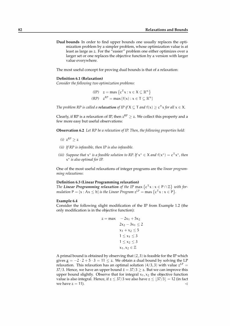
82 Relaxations and Bounds

Dual bounds In order to find upper bounds one usually replaces the opti-mization problem by a simpler problem, whose optimization value is atleast as large as z. For the “easier” problem one either optimizes over alarger set or one replaces the objective function by a version with largervalue everywhere.

The most useful concept for proving dual bounds is that of a relaxation:

Definition 6.1 (Relaxation)Consider the following two optimization problems:

(IP) z = maxcT x : x ∈ X ⊆ Rn

(RP) zRP = max f(x) : x ∈ T ⊆ Rn

The problem RP is called a relaxation of IP if X ⊆ T and f(x) ≥ cT x for all x ∈ X.

Clearly, if RP is a relaxation of IP, then zRP ≥ z. We collect this property and afew more easy but useful observations:

Observation 6.2 Let RP be a relaxation of IP. Then, the following properties hold:

(i) zRP ≥ z

(ii) If RP is infeasible, then IP is also infeasible.

(iii) Suppose that x∗ is a feasible solution to RP. If x∗ ∈ X and f(x∗) = cT x∗, thenx∗ is also optimal for IP.

One of the most useful relaxations of integer programs are the linear program-ming relaxations:

Definition 6.3 (Linear Programming relaxation)The Linear Programming relaxation of the IP max

cT x : x ∈ P ∩ Z

with for-

mulation P = x : Ax ≤ b is the Linear Program zLP = maxcTx : x ∈ P

.

Example 6.4Consider the following slight modification of the IP from Example 1.2 (theonly modification is in the objective function):

z = max − 2x1 + 5x2

2x2 − 3x1 ≤ 2

x1 + x2 ≤ 5

1 ≤ x1 ≤ 3

1 ≤ x2 ≤ 3

x1, x2 ∈ Z

A primal bound is obtained by observing that (2, 3) is feasible for the IP whichgives z = −2 · 2 + 5 · 3 = 11 ≤ z. We obtain a dual bound by solving the LPrelaxation. This relaxation has an optimal solution (4/3, 3) with value zLP =

37/3. Hence, we have an upper bound z = 37/3 ≥ z. But we can improve thisupper bound slightly. Observe that for integral x1, x2 the objective functionvalue is also integral. Hence, if z ≤ 37/3 we also have z ≤ ⌊37/3⌋ = 12 (in factwe have z = 11). ⊳

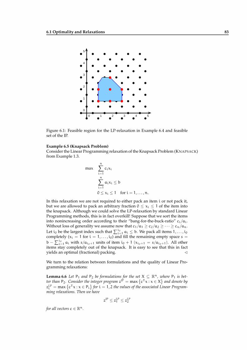
6.1 Optimality and Relaxations 83

0 1 2 3 4 5

0

1

2

3

4

5

b b b

b b b

b

Figure 6.1: Feasible region for the LP-relaxation in Example 6.4 and feasibleset of the IP.

Example 6.5 (Knapsack Problem)Consider the Linear Programming relaxation of the Knapsack Problem (KNAPSACK)from Example 1.3.

maxn∑

i=1

cixi

n∑

i=1

aixi ≤ b

0 ≤ xi ≤ 1 for i = 1, . . . , n.

In this relaxation we are not required to either pack an item i or not pack it,but we are allowed to pack an arbitrary fraction 0 ≤ xi ≤ 1 of the item intothe knapsack. Although we could solve the LP-relaxation by standard LinearProgramming methods, this is in fact overkill! Suppose that we sort the itemsinto nonincreasing order according to their “bang-for-the-buck-ratio” ci/ai.Without loss of generality we assume now that c1/a1 ≥ c2/a2 ≥ · · · ≥ cn/an.Let i0 be the largest index such that

∑i0

i=1 ai ≤ b. We pack all items 1, . . . , i0completely (xi = 1 for i = 1, . . . , i0) and fill the remaining empty space s =

b −∑i0

i=1 ai with s/ai0+1 units of item i0 + 1 (xi0+1 = s/ai0+1). All otheritems stay completely out of the knapsack. It is easy to see that this in factyields an optimal (fractional) packing. ⊳

We turn to the relation between formulations and the quality of Linear Pro-gramming relaxations:

Lemma 6.6 Let P1 and P2 be formulations for the set X ⊆ Rn, where P1 is bet-ter than P2. Consider the integer program zIP = max

cT x : x ∈ X

and denote by

zLPi = max

cT x : x ∈ Pi

for i = 1, 2 the values of the associated Linear Program-

ming relaxations. Then we have

zIP ≤ zLP1 ≤ zLP

2

for all vectors c ∈ Rn.


Proof: The result immediately follows from the fact that X ⊆ P1 ⊆ P2. 2

Example 6.7By using the formulation given in Example 6.4 we obtained an upper boundof 12 for the optimal value of the IP. If we use the ideal formulation

z = max 2x1 + 5x2

x1 + x2 ≤ 5

− x1 + x2 ≤ 1

1 ≤ x1 ≤ 3

1 ≤ x2 ≤ 3

x1, x2 ∈ Z

then we obtain the optimal solution for the relaxation (2, 3) with objectivefunction value 11. Thus, (2, 3) is an optimal solution for the original IP. ⊳

6.2 Combinatorial Relaxations

Sometimes the relaxation of a problem is a combinatorial optimization prob-lem. In this case we speak of a combinatorial relaxation. We have already seen anexample of such a problem in Example 6.5, where the LP-relaxation of KNAP-SACK turned out to be solvable by combinatorial methods. Combinatorialrelaxations are particularly nice if we can solve them in polynomial time.

Example 6.8 (Traveling Salesman Problem)Consider the TSP from Example 1.8.

minn∑

i=1

n∑

j=1

cijxij

∑

j:j6=i

xij = 1 for i = 1, . . . , n

∑

i:i6=j

xij = 1 for j = 1, . . . , n

∑

i∈S

∑

j∈S

xij ≤ |S| − 1 for all ∅ ⊂ S ⊂ V.(6.1)

x ∈ Bn(n−1)

Observe that if we drop the subtour elimination constraints (6.1) we have infact an assignment problem. An assignment in a directed graph G = (V, A) is asubset T ⊆ A of the arcs such that for each vertex v ∈ V we have either exactlyone outgoing arc or exactly one incoming arc. If we interprete the TSP in thegraph theoretic setting as we already did in Example 1.8 we get:

zTSP = minT⊆A

∑

(i,j)∈T

cij : T forms a tour

≥ minT⊆A

∑

(i,j)∈T

cij : T forms an assignment

⊳

6.2 Combinatorial Relaxations 85

Assignments in directed graphs are an analogon to matchings in undirectedgraphs. Matchings will play an important role througout our lecture notes,one reason being that a theorem by Edmonds about perfect matching polyhe-dra sparked the interest in polyhedral combinatorics.

Definition 6.9 (Matching, perfect matching)Let G = (V, E) be an undirected graph. A matching in G is a subset M ⊆ E ofthe edges of G such that no two edges in M share an endpoint. A matching is calledperfect, if for each v ∈ V there is one edge in M that is incident to v.

We remark here that we can decide in polynomial time whether a given graphhas a perfect matching. We can also compute a perfect matching of minimumweight in polynomial time.

Example 6.10 (Symmetric Traveling Salesman Problem)If in the TSP all distances are symmetric, that is cij = cji for all i, j, one speaksof a symmetric traveling salesman problem. This problem is best modelled on acomplete undirected graph G = (V, E). Each tour corresponds to a Hamilto-nian cycle in G, that is, a cycle which touches each vertex exactly once.

Observe that every TSP-tour (i.e., a Hamiltonian cycle) also contains a span-ning tree: If we remove one edge of the tour we obtain a path, a somewhatdegenerated spanning tree. Hence, the problem of finding a minimum span-ning tree in G = (V, E) with edge weights cij is a relaxation of the symmetricTSP:

zTSP ≥ zMST .

Recall that a minimum spanning tree can be computed in polynomial time forinstance by Kruskal’s algorithm. ⊳

The relaxation in the previous example can actually be used to prove an im-proved lower bound on the length of the optimal TSP-tour. Suppose that weare given an instance of the symmetric TSP where the distances satisfy thetriangle inequality, that is, we have

cij ≤ cik + ckj for all i, j, k.

Let T be a minimum spanning tree in G = (V, E) and let O denote the subset ofthe vertices which have an odd degree in T . Observe that O contains an evennumber of vertices, since the sum of all degrees in T sums up to 2(n−1) whichis even. Build a complete auxiliary graph H = (O, EO) where the weight ofan edge (u, v) coincides with the corresponding edgeweight in G. Since H

contains an even number of vertices and is complete, there exists a perfectmatching M in H. We can compute a perfect matching with minimum weightin H in polynomial time.

Lemma 6.11 The total weight c(M) =∑

e∈M ce of the minimum weight perfectmatching in H is at most 1/2zTSP .

Proof: Let O = (v1, . . . , v2k) be the sequence of odd degree vertices in T in theorder as they are visited by the optimum TSP-tour T∗. Consider the followingtwo perfect matchings in H:

M1 = (v1, v2), (v3, v4), . . . , (v2k−1, v2k)

M2 = (v2, v3), (v4, v5), . . . , (v2k, v1)


Figure 6.2 shows an illustration of the matchings M1 and M2. By the triangleinequality we have c(T∗) ≥ c(M1) + c(M2), so that at least one of the twomatchings has weight at most 1/2c(T∗). Thus, the minimum weight perfectmatching must have weight at most 1/2c(T∗). 2

v1 v2 v13 v14

v8 v9 v10 v3

v7 v11 v4

v15 v6 v5

(a) The TSP-tour.

v1 v2

v8 v3

v7 v4

v6 v5

(b) The two matchings

Figure 6.2: The two matchings constructed in Lemma 6.11 from the optimalTSP-tour. Matching M1 contains all the solid edges, M2 all the dashed ones.

Consider the graph G = (V, T ∪ M) obtained by adding the edges of the min-imum weight perfect matching M to the spanning tree T (see Figure 6.3(c)).Then, by construction any node in G has even degree. Since G is also con-nected (by the fact that it contains a spanning tree), it follows that G is Eule-rian (see e.g. [Har72, AMO93]), that is, it contains a cycle W which traversesevery edge exactly once. We have that

(6.2) c(W) =∑

w∈W

c(e) = c(T) + c(M) ≤ zTSP +1

2zTSP =

3

2zTSP .

In other words, 23c(W) ≤ zTSP is a lower bound for the optimal TSP-tour.

Moreover, we can convert the cycle W into a feasible tour T ′ by “shortcut-ting” the Eulerian cycle: we start to follow W at node 1. If we have reachedsome node i, we continue to the first subsequent node in W which we havenot visited yet. Due to the triangle inequality, the tour obtained this way has

6.2 Combinatorial Relaxations 87

weight at most that of W which by (6.2) is at most 3/2zTSP . The algorithm wejust described is known as Christofides’ algorithm. Figure 6.3 shows an exampleof the execution. Let T ′ be the tour found by the algorithm. By (6.2) we knowthat

2

3c(T ′) ≤ zTSP ≤ c(T ′).

We summarize our results:

Theorem 6.12 Given any instance of the symmetric TSP with triangle inequality,Christofides’ algorithm returns a tour of length at most 3/2zTSP . 2

1 2 3

4

5

6 7

8(a) The minimum spanning tree T.

1 2 3

4

5

6 7

8(b) The mimimum weight perfectmatching M on the vertices in T withodd degree.

1 2 3

4

5

6 7

8(c) The Eulerian graph G = (V,T∪M).

1 2 3

4

5

6 7

8(d) The approximate tour T ′ obtainedby shortcutting.

Figure 6.3: Example of the execution of Christofides’ algorithm for the sym-metric TSP with triangle inequality.

Christofides’ algorithm falls in the class of approximation algorithms. Those arealgorithms with provable worst-case performance guarantees.

Example 6.13 (1-Tree relaxation for the symmetric TSP)Another relaxation of the symmetric TSP is obtained by the following obser-vation: Every tour consists of two edges incident to node 1 and a path throughnodes 2, . . . , n (in some order). Observe that every path is also a tree. Call asubgraph T of G = (V, E) a 1-tree, if T consists of two edges incident on node 1


and the edges of a tree on nodes 2, . . . , n. We get:

zTSP = min

∑

e∈T

ce : T is a tour

≥ min

∑

e∈T

ce : T is a 1-tree

(6.3)

=: z1-Tree

The problem in (6.3) is called the 1-tree relaxation of the (symmetric) TSP. Ob-serve that we can find an optimal 1-tree easily in polynomial time: Let e, f ∈ E

with e 6= f be the two lightest edges incident with 1 and let H = G \ 1 bethe graph obtained from G by removing vertex 1. Then, the weight of an op-timal 1-tree is ce + cf + MST(H), where MST(H) is the weight of a minimumspanning tree in H. ⊳

6.3 Lagrangian Relaxation

The shortest path problem consists of finding a path of minimum weight be-tween given vertices s and t in a directed (or undirected) graph G. Here, weconsider the directed version, that is, we are given a directed graph G = (V, A)

with arc weights c : A → R+. We set up binary variables x(i, j) for (i, j) ∈ A

where x(i, j) = 1 if the path from s to t uses arc (i, j). Then, the shortest pathproblem (which is a special case of the minimum cost flow problem) can bewritten as the following IP:

min∑

(i,j)∈A

c(i, j)x(i, j)

∑

j:(j,i)∈A

x(j, i) −∑

j:(i,j)∈A

x(i, j) =

1 if i = t

−1 if i = s

0 otherwise(6.4)

x ∈ BA

The mass balance constraints (6.4) ensure that any feasible solution contains apath from s to t. Now, the shortest path problem can be solved very efficientlyby combinatorial algorithms. For instance, Dijkstra’s algorithm implementedwith Fibonacci-heaps runs in time O(m+n log n), where n = |V | and m = |A|.In other words, the above IP is “easy” to solve.

Now, consider the addition of the following constraint to the IP: in additionto the arc weights c : A → R+ we are also given a second set of arc costsd : A → R+. Given a budget B we wish to find a shortest (s, t)-path withrespect to the c-weights subject to the constraint that the d-cost of the pathis at most B. This problem is known as the resource constrained shortest pathproblem (RCSP).

Lemma 6.14 The RCSP is NP-hard to solve.

Proof: We show the claim by providing a polynomial time reduction fromKNAPSACK, which is known to be NP-complete to solve. Given an instanceof KNAPSACK with items 1, . . . , n we construct a directed acyclic graph for

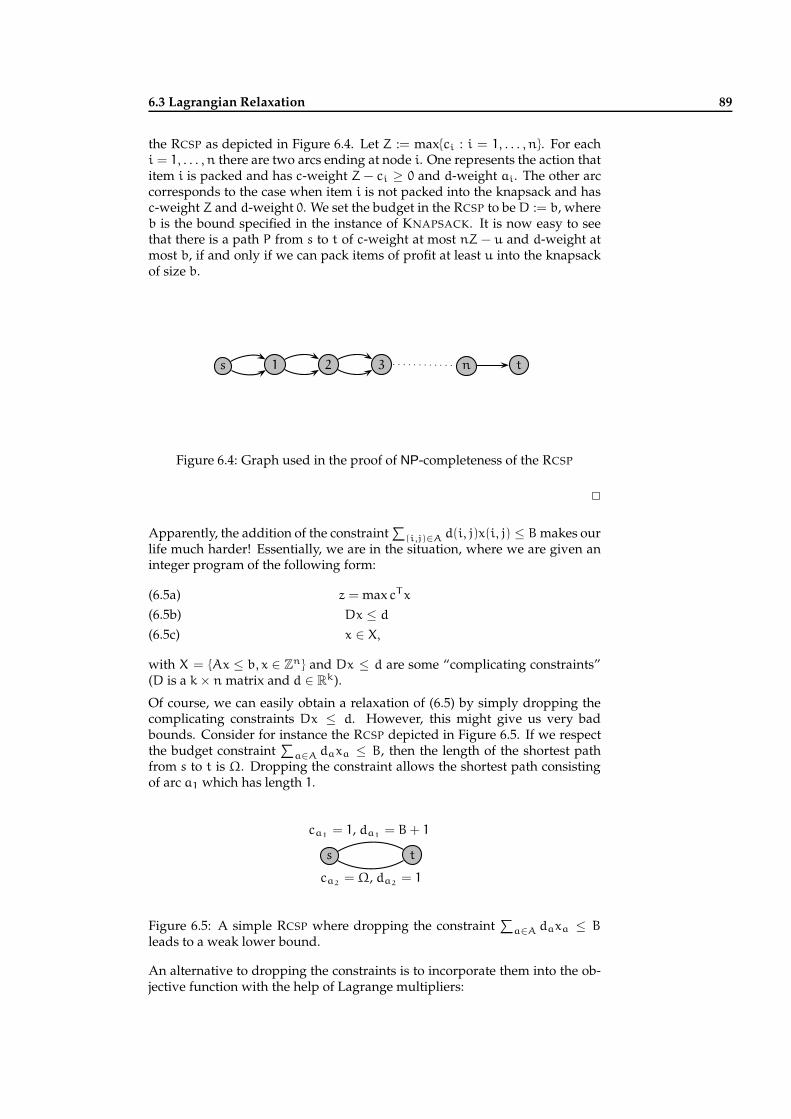
6.3 Lagrangian Relaxation 89

the RCSP as depicted in Figure 6.4. Let Z := maxci : i = 1, . . . , n. For eachi = 1, . . . , n there are two arcs ending at node i. One represents the action thatitem i is packed and has c-weight Z − ci ≥ 0 and d-weight ai. The other arccorresponds to the case when item i is not packed into the knapsack and hasc-weight Z and d-weight 0. We set the budget in the RCSP to be D := b, whereb is the bound specified in the instance of KNAPSACK. It is now easy to seethat there is a path P from s to t of c-weight at most nZ − u and d-weight atmost b, if and only if we can pack items of profit at least u into the knapsackof size b.

s 1 2 3 n t

Figure 6.4: Graph used in the proof of NP-completeness of the RCSP

2

Apparently, the addition of the constraint∑

(i,j)∈A d(i, j)x(i, j) ≤ B makes ourlife much harder! Essentially, we are in the situation, where we are given aninteger program of the following form:

z = max cT x(6.5a)

Dx ≤ d(6.5b)

x ∈ X,(6.5c)

with X = Ax ≤ b, x ∈ Zn and Dx ≤ d are some “complicating constraints”(D is a k × n matrix and d ∈ Rk).

Of course, we can easily obtain a relaxation of (6.5) by simply dropping thecomplicating constraints Dx ≤ d. However, this might give us very badbounds. Consider for instance the RCSP depicted in Figure 6.5. If we respectthe budget constraint

∑a∈A daxa ≤ B, then the length of the shortest path

from s to t is Ω. Dropping the constraint allows the shortest path consistingof arc a1 which has length 1.

s t

ca1= 1, da1

= B + 1

ca2= Ω, da2

= 1

Figure 6.5: A simple RCSP where dropping the constraint∑

a∈A daxa ≤ B

leads to a weak lower bound.

An alternative to dropping the constraints is to incorporate them into the ob-jective function with the help of Lagrange multipliers:


Definition 6.15 (Langrangean Relaxation)For a vector u ∈ Rm

+ the Lagrangean relaxation IP(u) for the IP (6.5) is defined asthe following optimization problem:

IP(u) z(u) = max cT x + uT (d − Dx)(6.6a)

x ∈ X(6.6b)

We note that there is no “unique” Lagrangean relaxation, since we are freeto include or exclude some constraints by the definition of the set X. Therelaxation IP(u) as defined above is usually called the relaxation obtained byrelaxing the constraints Dx ≤ d. The vector u ≥ 0 is referred to as the price, dualvariable or Lagrangian multiplier associated with the constraints Dx ≤ d.

Lemma 6.16 For any u ≥ 0, the problem IP(u) is a relaxation of the IP (6.5).

Proof: The fact that any feasible solution to the IP is also feasible to IP(u)

is trivial: X ⊇ x : Dx ≤ d, x ∈ X. If x is feasible for the IP, then Dx ≤ d ord−Dx ≥ 0. Since u ≥ 0 we have uT (d−Dx) ≥ 0 and thus cT x+uT (d−Dx) ≥cT x as required. 2

Consider again the RCSP. What happens, if we relax the budget constraint∑(i,j)∈A d(i, j)x(i, j) ≤ B? For u ∈ R+ the Lagrangean relaxation is

min∑

(i,j)∈A

c(i, j)x(i, j) + u

∑

(i,j)∈A

d(i, j)x(i, j) − B

∑

j:(j,i)∈A

x(j, i) −∑

j:(i,j)∈A

x(i, j) =

1 if i = t

−1 if i = s

0 otherwise

x ∈ BA.

If we rearrange the terms in the objective function, we obtain

∑

(i,j)∈A

(c(i, j) + ud(i, j))x(i, j) − uB.

In other words, IP(u) asks for a path P from s to t minimizing∑

a∈P(ca +

uda) − uB. If u ≥ 0 is fixed, this is the same as minimizing∑

a∈P(ca + uda).Hence, IP(u) is a (standard) shortest path problem with weights (c + ud) onthe arcs.

We have seen that IP(u) is a relaxation of IP for every u ≥ 0, in particularz(u) ≥ zIP. In order to get the best upper bound for zIP we can optimizeover u, that is, we solve the Lagrangean Dual Problem:

(6.7) (LD) wLD = min z(u) : u ≥ 0 .

Lemma 6.17 Let u ≥ 0 and x(u) be an optimal solution for IP(u). Suppose that thefollowing two conditions hold:

(i) Dx(u) ≤ d (that is, x is feasible for IP);

(ii) (Dx(u))i = di if ui > 0 (that is, x is complementary to u).


Then, x(u) is an optimal solution for the original IP.

Proof: Since x(u) is feasible for IP, we have cT x(u) ≤ z. On the other hand

z ≤ cTx(u) + uT (d − Dx(u)) (by Lemma 6.16)

= cT x(u) +

m∑

i=1

ui(Dx(u) − d)i︸︷︷︸=0

(by assumption (ii))

= cT x(u).

Thus, cT x(u) = z and x(u) is optimal as claimed. 2

Observe that if we dualize some equality constraints Dx = d, then the La-grange multiplier u is unrestricted in sign. In this case, the Lagrangean dualbecomes:

(6.8) (LD) wLD = min z(u) : u ∈ Rm .

Moreover, in this case, assumption (ii) of Lemma 6.17 is automatically satis-fied. Hence, if x(u) is feasible for the IP, then x(u) is also optimal.

What kind of bounds can we expect from LD? The following theorem ad-dresses this question:

Theorem 6.18 Let X = x : Ax ≤ b, x ∈ Zn where A and b are rational, and let z

denote the optimal value of the IP (6.5):

z = maxcT x : Dx ≤ x, x ∈ X

Then for the value of the Lagrangean dual as defined in (6.8) we have:

wLD = maxcTx : Dx ≤ d, x ∈ conv(X)

≥ z.

Proof: We have:

wLD = min z(u) : u ≥ 0

= minu≥0

maxcT x + uT (d − Dx) : x ∈ X

= minu≥0

max(c − DTu)T x + uT d : x ∈ X

= minu≥0

maxcT x + uT (d − Dx) : x ∈ conv(X)

,

where the last equality follows from the fact that the objective function is lin-ear. If X = ∅, then conv(X) = ∅ and wLD = −∞ since the inner maximum istaken over the empty set for every u. Since z = −∞, the result holds in thiscase.

If X 6= ∅ by Theorem 3.67 conv(X) is a rational polyhedron. Let xk, k ∈ K bethe extreme points and rj, j ∈ J be the extreme rays of conv(X). Fix u ≥ 0. Wehave

z(u) = maxcT x + uT (d − Dx) : x ∈ conv(X)

=

+∞ if (cT − uT D)rj > 0 for some j ∈ J

cT xk + uT (d − Dxk) for some k ∈ K otherwise.


Since for the minimization of z(u) it suffices to consider the case of finite z(u),we have

wLD = minu≥0:(cT −uT D)rj≤0 for j ∈ J

maxk∈K

cT xk + uT (d − Dxk)

We can restate the last problem as follows:

wLD = min t(6.9a)

t + (Dxk − d)T u ≥ cT xk for k ∈ K(6.9b)

(Drj)T u ≥ cT rj for j ∈ J(6.9c)

u ∈ Rm+ , t ∈ R(6.9d)

Observe that the problem (6.9) is a Linear Program. Hence by Linear Program-ming duality (cf. Theorem 2.8) we get:

wLD = max∑

k∈K

αkcT xk +∑

j∈J

βjcT rj

∑

k∈K

αk = 1

∑

k∈K

αk(Dxk − d) +∑

j∈J

βjrj ≤ 0

αk, βj ≥ 0, for k ∈ K, j ∈ J

Rearranging terms this leads to:

wLD = max cT

∑

k∈K

αkxk +∑

j∈J

βjrj

∑

k∈K

αk = 1

D

∑

k∈K

αkxk +∑

j∈J

βjrj

≤ d(∑

k∈K

αk)

αk, βj ≥ 0, for k ∈ K, j ∈ J

Since any point of the form∑

k∈K αkxk+∑

j∈J βjrj is in conv(X) (cf. Minkowski’s

Theorem), this gives us:

wLD = maxcT x : x ∈ conv(X), Dx ≤ d

.

This completes the proof. 2

Theorem 6.18 tells us exactly how strong the Langrangean dual is. Undersome circumstances, the bounds provided are no better than that of the LP-relaxation: More precisely, if conv(X) = x : Ax ≤ b, then by Theorem 6.18:wLD = max

cT x : Ax ≤ b, Dx ≤ d

and wLD is exactly the value of the LP-

relaxation of (6.5):

zLP = maxcT x : Ax ≤ b, Dx ≤ d

However, since

conv(X) = conv x ∈ Zn : Ax ≤ b ⊆ x ∈ Rn : Ax ≤ b ,


we always havez ≤ wLD ≤ zLP,

and in most cases we will have wLD < zLP. In Chapter 11 we will learn moreabout Lagrangean duality. In particular, we will be concerned with the ques-tion how to solve the Lagrangean dual.

Example 6.19 (Lagrangean relaxation for the symmetric TSP)The symmetric TSP can be restated as the following Integer Linear Program:

zTSP = min∑

e∈E

cexe(6.10a)

∑

e∈δ(i)

xe = 2, for all i ∈ V(6.10b)

∑

e∈E(S)

xe ≤ |S| − 1, for all 2 ≤ |S| ≤ |V | − 1(6.10c)

x ∈ BE(6.10d)

Here δ(i) denotes the set of edges incident with node i and E(S) is the set ofedges that have both endpoints in S.

Let x be any feasible solution to the LP-relaxation of (6.10). Let S ⊂ V with2 ≤ |S| ≤ |V | − 1 and S = V \ S. We denote by (S, S) the set of edges whichhave one endpoint in S and the other one in S. Due to the constraints (6.10b)we have:

|S| =1

2

∑

i∈S

∑

j∈δ(i)

xe.

Hence,

|S| −∑

e∈E(S)

xe =1

2

∑

i∈S

∑

j∈δ(i)

xe −∑

e∈E(S)

xe

=1

2

∑

e∈(S,S)

xe.(6.11)

By the analogous calculation we get

|S| −∑

e∈E(S)

xe =1

2

∑

e∈(S,S)

xe.(6.12)

From (6.11) and (6.12) we conclude that∑

e∈E(S) xe ≤ |S| − 1 if and only if∑

e∈E(S) xe ≤ |S| − 1. This calculation shows that in fact half of the subtourelimination constraints (6.10b) are redundant. As a consequence, we can dropall subtour constraints with 1 ∈ S. This gives us the equivalent integer pro-gram:

zTSP = min∑

e∈E

cexe(6.13a)

∑

e∈δ(i)

xe = 2, for all i ∈ V(6.13b)

∑

e∈E(S)

xe ≤ |S| − 1, for all 2 ≤ |S| ≤ |V | − 1, 1 /∈ S(6.13c)

x ∈ BE(6.13d)


If we sum up all the constraints (6.13b) we get 2∑

e∈E xe = 2n, since everyedge is counted exactly twice. Now comes our Lagrangean relaxation: We du-alize all degree constraints (6.13b) in (6.13) but leave the degree constraint fornode 1. We also add the constraint

∑e∈E xe = n. This gives us the following

relaxation:

z(u) = min∑

(i,j)∈E

(cij − ui − uj)xe + 2∑

i∈V

ui(6.14a)

∑

e∈δ(1)

xe = 2(6.14b)

∑

e∈E(S)

xe ≤ |S| − 1, for all 2 ≤ |S| ≤ |V | − 1, 1 /∈ S(6.14c)

∑

e∈E

xe = n(6.14d)

x ∈ BE(6.14e)

Let us have a closer look at the relaxation (6.14). Every feasible solution T hastwo edges incident with node 1 by constraint (6.14b). By constraint (6.14d),the solution must consist of exactly n edges and hence has a cycle. By con-straints (6.14c), T can not contain a cycle that does not contain node 1. Thus,if we remove one edge incident to 1, then T is cycle free and must contain aspanning tree on the vertices 2, . . . , n. To summarize, the feasible solutionsfor (6.14) are exactly the 1-trees. We have already seen in Example 6.13 thatwe can compute a minimum weight 1-tree in polynomial time. Hence, therelaxation (6.14) is particularly interesting. ⊳

6.4 Duality

As mentioned at the beginning of Chapter 6, for Linear Programs the Dual-ity Theorem is a convenient way of proving optimality or, more general, forproving upper and lower bounds for an optimization problem. We are nowgoing to introduce the concept of duality in a more general sense.

Definition 6.20 ((Weak) dual pair of optimization problems)The two optimization problems:

(IP) z = max c(x) : x ∈ X

(D) w = min ω(y) : y ∈ Y

for a (weak-) dual pair, if c(x) ≤ ω(y) for all x ∈ X and all y ∈ Y. If z = w, thenwe say that the problem form a strong-dual pair.

By the Duality Theorem of Linear Programming, the both problems

(P) max cT x : x ∈ Ax ≤ b

(D) min bTy : y ∈ Q

form a strong-dual pair.

6.4 Duality 95

Example 6.21 (Matching and vertex cover)Given an undirected graph G = (V, E), the following two problems form aweak-dual pair:

max |M| : M ⊆ E is a matching in G

min |C| : C ⊆ V is a vertex cover in G

In fact, let M ⊆ E be a matching in G and C ⊆ V a vertex cover. Since M

is a matching, the edges in M do not share a common endpoint. Thus, sinceC must contain at least one endpoint for each e ∈ M (and all of the 2|M|

endpoints are different as we have just seen), we get that |C| ≥ |M|.

Do the two problems form a strong-dual pair? The answer is no: Figure 6.6shows an example of a graph, where the maximum size matching has cardi-nality 1, but the minimum vertex cover has size 2. After a moment’s thought,it would be very surprising if the two problems formed a strong-dual pair:the vertex-cover problem is NP-hard to solve, whereas the matching problemis solvable in polynomial time. ⊳

2

1 3

e1 e2

e3

Figure 6.6: A graph where the maximum matching has size 1, but the mini-mum vertex cover has size 2.

Lemma 6.22 The Integer Linear Program maxcT x : Ax ≤ b, x ∈ Zn

and the

Linear Program minbTy : AT y ≥ c, y ∈ Rm

+

form a weak dual pair. Moreover,

also the two Integer Linear Programs

maxcT x : Ax ≤ b, x ∈ Zn

minbTy : ATy ≥ c, y ∈ Zm

+

form a weak dual pair.

Proof: We have


≤ max

cTx : Ax ≤ b, x ∈ Rn

= minbTy : ATy ≥ c, y ∈ Rm

+

≤ minbTy : AT y ≥ c, y ∈ Zm

+

,

where the equality follows from the Duality Theorem of Linear Program-ming. 2

Example 6.23 (Matching and vertex cover (continued))We formulate the maximum cardinality matching problem as an integer pro-gram:

z = max∑

e∈E

xe(6.15)

∑

e:e∈δ(v)

xe ≤ 1, for all v ∈ V(6.16)

x ∈ BE(6.17)


Let zLP be the value of the LP-relaxation of (6.15) obtained by dropping theintegrality constraints. The dual of the LP-relaxation is

wLP = min∑

v∈V

yv(6.18)

xu + xv ≥ 1, for all e = (u, v) ∈ E(6.19)

x ≥ 0.(6.20)

If we put integrality constraints on (6.18) we obtain the vertex cover problem.Let w denote the optimal value of this problem. We then have z ≤ zLP =

wLP ≤ w. This is an alternative proof for the fact that the matching problemand the vertex cover problem form a weakly dual pair.

Consider again the graph depicted in Figure 6.6. We have already seen thatfor this graph z = 1 and w = 2. Moreover, the Linear Programming relaxationis

maxxe1+ xe2

+ xe3

xe1+ xe2

≤ 1

xe1+ xe3

≤ 1

xe2+ xe3

≤ 1

xe1, xe2

, xe3≥ 0

The vector xe1= xe2

= xe3= 1/2 is feasible for this relaxation with objective

function value 3/2. The dual of the LP is

miny1 + y2 + y3

y1 + y2 ≥ 1

y2 + y3 ≥ 1

y1 + y3 ≥ 1

y1, y2, y3 ≥ 0

so that y1 = y2 = y3 = 1/2 is feasible for the dual. Hence we have zLP =

wLP = 3/2. ⊳

Dynamic Programming

7.1 Shortest Paths Revisited

Suppose that we are given a directed graph G = (V, A) with arc lengthsc : A → R+ and we wish to compute a shortest paths from a distinguishedsource node s to all other vertices v ∈ V . Let d(v) denote the shortest pathdistance from s to v with respect to c.

Suppose the shortest path from s to v passes through some intermediatenode u (see Figure 7.1 for an illustration). What can we say about the paths Psu

and Puv from s to u and from u to v? Clearly, Psu must be a shortest (s, u)-path since otherwise we could replace it by a shorter one which together withPuv would form a shorter path from s to v. The same arguments show thatPuv must be a shortest (u, v)-path.

The above observations are known as the Bellman principle of optimality: anysubpath (any partial solution) of a shortest path (of an optimal solution) mustbe a shortest path (an optimal solution of a subproblem) itself.

Let v ∈ V \ s. If we apply the Bellman principle to all predecessors u of v,that is, to all u such that (u, v) ∈ A we get the following recurrences for theshortest path distances:

(7.1) d(v) = minu:(u,v)∈A

d(u) + c(u, v).

Equation (7.1) states that, if we know the shortest path distance d(u) from s

to all predecessors u of v, then we can easily compute the shortest path dis-tance d(v). Unfortunately, it may be the case that in order to compute d(u) we

s

u

v

Figure 7.1: A shortest path from s to v that passes through the intermediatenode u. The subpath from s to u must be a shortest (s, u)-path.

98 Dynamic Programming

also need d(v), because v in turn is a predecessor of u. So, for general graphs,(7.1) does not yet give us a method for solving the shortest path problem.

There is, however, one important class of graphs, where (7.1) can be used suchas to obtain a very efficient algorithm.

Definition 7.1 (Directed acyclic graph (DAG))A directed acyclic graph (DAG) is a graph that does not contain a directed cycle.

DAGs allow a special ordering of the vertices defined below:

Definition 7.2 (Topological sorting)Let G = (V, A) be a directed graph. A bijection f : V → 1, . . . , n is called a topo-logical sorting of G if for all (u, v) ∈ A we have f(u) < f(v).

The proof of the following fact is left as an exercise:

Theorem 7.3 Let G = (V, A) be a directed graph. Then, G has a topological sortingif and only if G is acyclic. If G is acyclic, the topological sorting can be computed inlinear time.

Proof: Exercise. 2

Suppose that G is a DAG and that f is a topological sorting (which by theprevious theorem can be obtained in linear time O(n + m), where n = |V |

and m = |A|). For the sake of a simpler notation we assume that the verticesare already numbered v1, . . . , vn according to the topological sorting, that is,f(vi) = i. We can now use (7.1) by computing d(vi) = 0 in order of increas-ing i = 1, . . . , n. In order to compute d(vi) we need values d(vj) where j < i

and these have already been computed. Thus, in case of a DAG (7.1) leads toan algorithm which can be seen to run in total time O(n + m).

In our algorithm above we have calculated the solution value of a problem re-cursively from the optimal values of slightly different problems. This methodis known as dynamic programming. We will see in this chapter that this methodcan be used to obtain optimal solutions to many problems. As a first step wego back to the shortest path problem but we now consider the case of generalgraphs. As we have already remarked above, the recursion (7.1) is not directlyuseful in this case. We need to somehow enforce an ordering on the verticessuch as to get a usable recursion.

Let dk(v) be the length of a shortest path from s to v using at most k arcs.Then, we have

(7.2) dk(v) = min

dk−1(v), minu:(u,v)∈A

dk−1(u) + c(u, v)

.

Now, the recurrence (7.2) gives us a way to compute the shortest path dis-tances in time O((n + m)m). We first compute d1(v) for all v which is easy.Once we know all values dk−1, we can use (7.2) to compute dk(v) for all v ∈ V

in time O(n+m) (every arc has to be considered exactly once). Since the rangeof k is from 1 to n−1 (every path with at least n arcs contains a cycle and thuscan not be shortest), we get the promised running time of O(n(n + m)) =

O(n2 + nm).

The general tune of a dynamic programming algorithm is the following: Wecompute a solution value recursively from the values of modified problems.

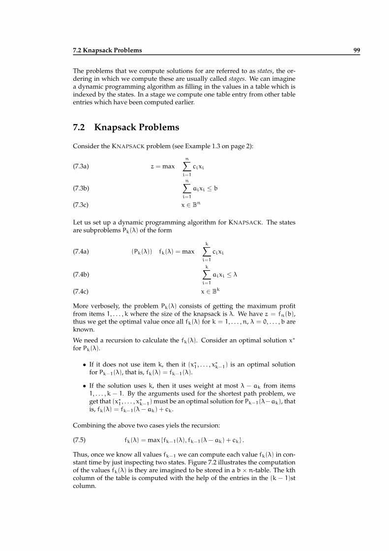
7.2 Knapsack Problems 99

The problems that we compute solutions for are referred to as states, the or-dering in which we compute these are usually called stages. We can imaginea dynamic programming algorithm as filling in the values in a table which isindexed by the states. In a stage we compute one table entry from other tableentries which have been computed earlier.

7.2 Knapsack Problems

Consider the KNAPSACK problem (see Example 1.3 on page 2):

z = maxn∑

i=1

cixi(7.3a)

n∑

i=1

aixi ≤ b(7.3b)

x ∈ Bn(7.3c)

Let us set up a dynamic programming algorithm for KNAPSACK. The statesare subproblems Pk(λ) of the form

(Pk(λ)) fk(λ) = maxk∑

i=1

cixi(7.4a)

k∑

i=1

aixi ≤ λ(7.4b)

x ∈ Bk(7.4c)

More verbosely, the problem Pk(λ) consists of getting the maximum profitfrom items 1, . . . , k where the size of the knapsack is λ. We have z = fn(b),thus we get the optimal value once all fk(λ) for k = 1, . . . , n, λ = 0, . . . , b areknown.

We need a recursion to calculate the fk(λ). Consider an optimal solution x∗

for Pk(λ).

• If it does not use item k, then it (x∗1, . . . , x∗

k−1) is an optimal solutionfor Pk−1(λ), that is, fk(λ) = fk−1(λ).

• If the solution uses k, then it uses weight at most λ − ak from items1, . . . , k − 1. By the arguments used for the shortest path problem, weget that (x∗

1, . . . , x∗k−1) must be an optimal solution for Pk−1(λ−ak), that

is, fk(λ) = fk−1(λ − ak) + ck.

Combining the above two cases yiels the recursion:

(7.5) fk(λ) = max fk−1(λ), fk−1(λ − ak) + ck .

Thus, once we know all values fk−1 we can compute each value fk(λ) in con-stant time by just inspecting two states. Figure 7.2 illustrates the computationof the values fk(λ) is they are imagined to be stored in a b × n-table. The kthcolumn of the table is computed with the help of the entries in the (k − 1)stcolumn.


1 2 k − 1 k

fk−1(λ − ak)

fk−1(λ)fk(λ)

Figure 7.2: Computation of the values fk(λ) in the dynamic programmingalgorithm for KNAPSACK.

The recursion (7.5) gives a dynamic programming algorithm for KNAPSACK

which runs in total time O(nb) (it is easy to actually set the binary variablesaccording to the results of the recusion). Observe that this running time isnot polynomial, since the encoding length of an instance of KNAPSACK is onlyO(n + n log amax + n log cmax + log b).

Let us now consider a generalized version of KNAPSACK, where we are al-lowed to pack more than one copy of an item. The Integer Knapsack Problem(INTEGERKNAPSACK) is:

z = maxn∑

i=1

cixi(7.6a)

n∑

i=1

aixi ≤ b(7.6b)

x ∈ Zn+(7.6c)

Analogous to KNAPSACK we can define

(Pk(λ)) gk(λ) = maxk∑

i=1

cixi(7.7a)

k∑

i=1

aixi ≤ λ(7.7b)

x ∈ Zk+(7.7c)

As before, gn(b) gives us the optimal solution for the whole problem. Weneed a recursion to compute the gk(λ), k = 1, . . . , n, λ = 0, . . . , b.

Let x∗ be an optimal solution for Pk(λ). Suppose that x∗k = t for some integer

t ∈ Z+. Then, x∗ uses space at most λ − tak for the items 1, . . . , k − 1. Itfollows that (x∗

1, . . . , x∗k−1) must be an optimal solution for Pk(λ − tak). These

observations give us the following recursion:

(7.8) gk(λ) = maxt=0,...,⌊λ/ak⌋

ckt + gk−1(λ − tak) .

Notice that ⌊λ/ak⌋ ≤ b, since ak is an integer. Thus (7.8) shows how to com-pute gk(λ) in time O(b). This yields an overall time of O(nb2) for the nb val-ues gk(λ).

Let us now be a bit smarter and get a dynamic programming algorithm witha better running time. The key is to accomplish the computation of gk(λ) by

7.3 Problems on Trees 101

inspecting only a constant (namely two) previously computed values insteadof Θ(b) as in (7.8).

Again, let x∗ be an optimal solution for Pk(λ).

• If x∗k = 0, then gk(λ) = gk−1(λ).

• If x∗k = t + 1 for some t ∈ Z+, then (x∗

1, . . . , x∗k − 1) must be an optimal

solution for Pk(λ − ak).

The above two cases can be combined into the new recursion

(7.9) gk(λ) = max gk−1(λ), gk(λ − ak) + ck .

Observe that the recursion allows us to compute all gk(λ) if we compute themin the order k = 1, . . . , n and λ = 0, . . . , b. The total running time is O(nb)

which is the same as for KNAPSACK.

7.3 Problems on Trees

Problems defined on tree structures are natural candidates for dynamic pro-gramming algorithms. Suppose that we are given a tree T = (V, E) with root r

(cf. Figure 7.3). The ubiquitous theme for applying dynamic programming al-gorithms on tree structured problems is to solve the problem on T by solvingproblems on Tvi

, i = 1, . . . , k, where vi are the children of r and Tviis the

subtree of T rooted at vi.

r

v1 v2 · · · vk

Figure 7.3: Recursive solution of a problem on a rooted tree.

We illustrate the construction by considering a specific problem. Suppose thatwe are given a tree T = (V, E) with root r profits/costs p : V → R for thevertices. The goal is to find a (possibly empty) subtree T ′ rooted at r (whichmay correspond to some distribution center) such as to maximize the profit,that is, maximize

f(T ′) :=∑

v∈V(T ′)

p(v)

For a node v ∈ V let g(v) denote the optimal net profit of a subtree of Tv (thesubtree rooted at v). Thus, the optimal solution (value) is obtained from g(r).

We now show how to build a recursion in order to compute g(v) for all ver-tices v ∈ V . The recursion scheme is typical for dynamic programming algo-rithms on trees. We compute the values g(v) “bottom up” starting from theleaves. If v is a leaf, then

(7.10) g(v) = max 0, p(v) .

Suppose now that v has the children v1, . . . , vk and that we have already com-puted g(vi), i = 1, . . . , k. Any subtree T ′ of Tv is composed of (possibly empty)


subtrees of Tvi. Consider an optimal subtree T∗ of Tv. Any subtree of Tvi

in-cluded in T∗ must be an optimal subtree of Tvi

(by Bellman’s principle). Thus,we get

(7.11) g(v) = max

0, p(v) +

k∑

i=1

g(vi)

,

where the 0 in the maximum covers the case that the optimal subtree of Tv isempty. Equations (7.10) and (7.11) now give us a way to compute all the g(v)

in time O(n), where n = |V | is the number of vertices in T .

We now consider a generalization of the problem. In addition to the prof-its/costs on the vertices, we are also given costs c : E → R+ on the edges (thevertices correspond to customers which may be connected by a network thathas to be built at some cost). The problem is now to select a subtree whichmaximizes the net profit:

h(T ′) :=∑

v∈V(T ′)

p(v) −∑

e∈E(T ′)

c(e).

Again, we define h(v) to be the optimal profit obtainable in the subtree rootedat v ∈ V . The problem once more easy for the leaves:

(7.12) h(v) = max 0, p(v) .

Now consider a non-leaf v with children v1, . . . , vk. An optimal subtree T∗

of Tv is once more composed of optimal subtrees of the Tvi. But now the sub-

tree Tvimay only be nonempty if the edge (v, vi) is contained in T∗. This gives

us the recursion:

(7.13) h(v) = max

0, maxx∈Bk

k∑

i=1

(h(vi) − c(v, vi))xi

.

Here, xi ∈ B is a decision variable which indicates whether we should includethe optimal subtree of Tvi

in the solution for Tv. It seems like (7.13) forces usto evaluate 2k values in order to compute h(v), if v has k children. However,the problem

maxx∈Bk

k∑

i=1

(h(vi) − c(v, vi))xi

can be solved easily in time O(k): Set xi = 1, if h(vi) − c(v, vi) > 0 andxi = 0 otherwise. Let deg+

(v) denote the number of children of v in T . Then,∑v∈V deg+

(v) = n − 1, since every edge is counted exactly once. Thus, thedynamic programming algorithm for the generalized problem runs in timeO(n

∑v∈V deg+

(v)) = O(n2).

Branch and Bound

8.1 Divide and Conquer

Suppose that we would like to solve the problem

z = maxcT x : x ∈ S

.

If the above problem is hard to solve, we might try to break it into smallerproblems which are easier to solve.

Observation 8.1 If S = S1∪· · ·∪Sk and zi = maxcT x : x ∈ Si

for i = 1, . . . , k

then z = maxzi : i = 1, . . . , k

.

Although Observation 8.1 is (almost) trivial, it is the key to branch and boundmethods which turn out to be effective for many integer programming prob-lems.

The recursive decomposition of S into smaller problems can be representedby an enumeration tree. Suppose that S ⊆ B3. We first divide S into S0 and S1,where

S0 = x ∈ S : x1 = 0

S1 = x ∈ S : x1 = 1

The sets S0 and S1 will be recursively divided into smaller sets as shown inthe enumeration tree in Figure 8.1.

As a second example consider the tours of a TSP on four cities. Let S denotethe set of all tours. We first divide S into three pieces, S12, S13 and S14, whereS1i ⊂ S is the set of all tours which from city 1 go directly to city i. Set S1i

in turn is divided into two pieces S1i,ij, j 6= 1, i, where S1i,ij is the set of alltours in Si1 which leave city i for city j. The recursive division is depicted inthe enumeration tree in Figure 8.2. The leaves of the tree correspond to the(4 − 1)! = 3! = 6 possible permutations of 1, . . . , 4 which have 1 at the firstplace.

8.2 Pruning Enumeration Trees

It is clear that a complete enumeration soon becomes hopeless even for prob-lems of medium size. For instance, in the TSP the complete enumeration tree

104 Branch and Bound

S

S0

x1 = 0

S00

x2 = 0

S000

x3 = 0

S001

x3 = 1

S01

x2 = 1

S010

x3 = 0

S011

x3 = 1

S1

x1 = 1

S10

x2 = 0

S100

x3 = 0

S101

x3 = 1

S11

x2 = 1

S110

x3 = 0

S111

x3 = 1

Figure 8.1: Enumeration tree for a set S ⊆ B4.

S

S12

S12,23 S12,24

S13

S13,32 S13,34

S14

S14,42 S14,43

Figure 8.2: Enumeration tree for the TSP on four cities.

8.2 Pruning Enumeration Trees 105

would have (n − 1)! leaves and thus for n = 60 would be larger than theestimated number of atoms in the universe1.

The key to efficient algorithms is to “cut off useless parts” of an enumerationtree. This is where bounds (cf. Chapter 6) come in. The overall scheme ob-tained is also referred to as implicit enumeration, since most of the time not allof the enumeration tree is completely unfolded.

Observation 8.2 Let S = S1∪. . . Sk and zi = maxcT x : x ∈ Si

for i = 1, . . . , k

then z = maxzi : i = 1, . . . , k

. Suppose that we are given zi and zi for i =

1, . . . , k withzi ≤ zi ≤ zi for i = 1, . . . , k.

Then for z = maxcT x : x ∈ S

it is true that:

max

zi : i = 1, . . . , k≤ z ≤ max

zi : i = 1, . . . , k

The above observation enables us to deduce rules how to prune the enumerationtree.

Observation 8.3 (Pruning by optimality) If zi = zi for some i, then the optimalsolution value for the ith subproblem zi = max

cT x : x ∈ Si

is known and there is

no need to subdivide Si into smaller pieces.

As an example consider the situation depicted in Figure 8.3. The set S is di-vided into S1 and S2 with the upper and lower bounds as shown.

S

S1 S2

z = 10

z = 30

z1 = 20

z1 = 20

z2 = 15

z2 = 25

→ S

S1 S2

z = 20

z = 25

z2 = 15

z2 = 25

Figure 8.3: Pruning by optimality.

Since z1 = z1, there is no need to further explore the branch rooted at S1. So,this branch can be pruned by optimality. Moreover, Observation 8.2 allows usto get new lower and upper bounds for z as shown in the figure.

Observation 8.4 (Pruning by bound) If zi < zj for some i 6= j, then the optimalsolution value for the ith subproblem zi = max

cTx : x ∈ Si

can never be an opti-

mal solution of the whole problem. Thus, there is no need to subdivide Si into smallerpieces.

Consider the example in Figure 8.4. Since z1 = 20 < 21 = z2, we can concludethat the branch rooted at S1 does not contain an optimal solution: any solutionin this branch has objective function value at most 20, whereas the branchrooted at S2 contains solutions of value at least 21. Again, we can stop toexplore the branch rooted at S1.

We list one more generic reason which makes the exploration of a branch un-necessary.

Observation 8.5 (Pruning by infeasibility) If Si = ∅, then there is no need tosubdivide Si into smaller pieces, either.

1The estimated number of atoms in the universe is 1080 .


S

S1 S2

z = 10

z = 30

z1 = 15

z1 = 20

z2 = 21

z2 = 25

→ S

S1 S2

z = 21

z = 25

z2 = 21

z2 = 25

Figure 8.4: Pruning by bound.

The next section will make clear how the case of infeasibility can occur ina branch and bound system. We close this section by showing an examplewhere no pruning is possible. Consider the partial enumeration tree in Fig-ure 8.5, where again we have divided the set S into the sets S1 and S2 with thebounds as shown.

S

S1 S2

z = 10

z = 30

z1 = 15

z1 = 20

z2 = 17

z2 = 25

→ S

S1 S2

z = 17

z = 25

z1 = 15

z1 = 20

z2 = 17

z2 = 25

Figure 8.5: No pruning possible.

Although the lower and upper bounds for the subproblems allow us to getbetter bounds for the whole problem, we still have to explore both subtrees.

8.3 LP-Based Branch and Bound: An Example

The most common way to solve integer programs is to use an implicit enu-meration scheme based on Linear Programming. Lower bounds are providedby LP-relaxations and branching is done by adding new constraints. We illus-trate this procedure for a small example. Figure 8.6 shows the evolution of thecorresponding branch-and-bound-tree.

Consider the integer program

z = max 4x1 − x2(8.1a)

3x1 − 2x2 + x3 = 14(8.1b)

x2 + x4 = 3(8.1c)

2x1 − 2x2 + x5 = 3(8.1d)

x ∈ Z5+(8.1e)

Bounding The first step is to get upper and lower bounds for the optimalvalue z. An upper bound is obtained by solving the LP-relaxation of (8.1).This LP has the optimal solution x = (4.5, 3, 6.5, 0, 0). Hence, we get the upperbound z = 15. Since we do not have any feasible solution yet, by conventionwe use z = −∞ as a lower bound.

Branching In the current situation (see Figure 8.6(a)) we have z < z, so wehave to branch, that is, we have to split the feasible region S. A common wayto achieve this is to take an integer variable xj that is basic but not integral and

8.3 LP-Based Branch and Bound: An Example 107

Sz = −∞

z = 15

(a) Initial tree

S

S1

x1 ≤ 4

S2

x1 ≥ 5

z = −∞

z =

Pruned by infeasibility

(b) Node S2 is pruned by infea-sibility.

S

S1

x1 ≤ 4

S2

x1 ≥ 5

z = −∞

z = 13.5

z1 = −∞

z1 = 13.5Pruned by infeasibility

(c) After the LP-relaxation of S2

is solved, we get a new upperbound.

S

S1

x1 ≤ 4

S11

x2 ≤ 2

S12

x2 ≥ 3

S2

x1 ≥ 5

z = −∞

z = 13.5

z1 = −∞

z1 = 13.5Pruned by infeasibility

(d) Branching on variable x2

leads to two new subproblems.

S

S1

x1 ≤ 4

S11

x2 ≤ 2

S12

x2 ≥ 3

S2

x1 ≥ 5

z = 13

z = 13.5

z1 = 13

z1 = 13.5

z12 = 13

z12 = 13


Pruned by optimality

(e) Problem S12 has an inte-gral optimal solution, so we canprune it by optimality. Thisalso gives the first finite lowerbound.

S

S1

x1 ≤ 4

S11

x2 ≤ 2

S12

x2 ≥ 3

S2

x1 ≥ 5

z = 13

z = 13.5

z1 = 13

z1 = 13.5

z12 = 13

z12 = 13

z11 = −∞

z11 = 12


Pruned by optimalityPruned by bound

(f) Problem S11 can be prunedby bound, since z11 = 12 <

13 = z.

Figure 8.6: Evolution of the branch-and-bound-tree for the example. The ac-tive nodes are shown in white.


set:

S1 = S ∩ x : xj ≤ ⌊xj⌋S2 = S ∩ x : xj ≥ ⌈xj⌉

Clearly, S = S1 ∪ S2 and S1 ∩ S2 = ∅. Observe that due to the above choiceof branching, the current optimal basic solution x is not feasible for eithersubproblem. If there is no degeneracy (i.e., multiple optimal LP solutions),then we get max

z1, z2

< z, which means that our upper bound decreases

(improves).

In the concrete example we choose variable x1 where x1 = 4.5 and set S1 =

S ∩ x : x1 ≤ 4 and S2 = S ∩ x : x1 ≥ 5.

Choosing an active node The list of active problems (nodes) to be examinedis now S1, S2. Suppose we choose S2 to be explored. Again, the first step is toobtain an upper bound by solving the LP-relaxation:

z = max 4x1 − x2(8.2a)

3x1 − 2x2 + x3 = 14(8.2b)

x2 + x4 = 3(8.2c)

2x1 − 2x2 + x5 = 3(8.2d)

x1 ≥ 5(8.2e)

x ≥ 0(8.2f)

It turns out that (8.2) is infeasible, so S2 can be pruned by infeasibility (seeFigure 8.6(b)).

Choosing an active node The only active node at the moment is S1. So, wechoose S1 to be explored. We obtain an upper bound z1 by solving the LP-relaxation

z = max 4x1 − x2(8.3a)

3x1 − 2x2 + x3 = 14(8.3b)

x2 + x4 = 3(8.3c)

2x1 − 2x2 + x5 = 3(8.3d)

x1 ≤ 4(8.3e)

x ≥ 0.(8.3f)

An optimal solution for (8.3) is x2 = (4, 2.5, 7, 4, 0) with objective functionvalue 13.5. This allows us to update our bounds as shown in Figure 8.6(c).

This time we choose to branch on variable x2, since x22 = 2.5. The two subprob-

lems are defined on the sets S11 = S1 ∩ x : x2 ≤ 2 and S12 = S1 ∩ x : x2 ≥ 3,see Figure 8.6(d).

8.4 Techniques for LP-based Branch and Bound 109

Choosing an active node The list of active nodes is S12 and S22. We choose S22

and solve the LP-relaxation

z = max 4x1 − x2(8.4a)

3x1 − 2x2 + x3 = 14(8.4b)

x2 + x4 = 3(8.4c)

2x1 − 2x2 + x5 = 3(8.4d)

x1 ≤ 4(8.4e)

x2 ≥ 3(8.4f)

x ≥ 0.(8.4g)

An optimal solution of (8.4) is x12 = (4, 3, 8, 1, 0) with objective functionvalue 13. As the solution is integer, we can prune S12 by optimality. Moreover,we can also update our bounds as shown in Figure 8.6(e).

Choosing an active node At the moment we only have one active node: S11.The corresponding LP-relaxation is

z = max 4x1 − x2(8.5a)

3x1 − 2x2 + x3 = 14(8.5b)

x2 + x4 = 3(8.5c)

2x1 − 2x2 + x5 = 3(8.5d)

x1 ≤ 4(8.5e)

x2 ≤ 2(8.5f)

x ≥ 0,(8.5g)

which has x11 = (3.5, 2, 7.5, 1, 0) as an optimal solution. Hence, z11 = 12

which is strictly smaller than z = 13. This means that S11 can be pruned bybound.

8.4 Techniques for LP-based Branch and Bound

The previous section contained an example for an execution of an LP-basedbranch and bound algorithm. While the basic outline of such an algorithmshould be clear, there are a few issues that need to be taken into account inorder to obtain the best possible efficiency.

8.4.1 Reoptimization

Consider the situation in the example from the previous section when wewanted to explore node S1. We had already solved the initial LP for S.The only difference between LP(S) and LP(S1) is the presence of the con-straint x1 ≤ 4 in LP(S1). How can we solve LP(S1) without starting fromscratch?

The problem LP(S) is of the form maxcT x : Ax = b, x ≥ 0

. An optimal basis

for this LP is B = x1, x2, x3 with solution x∗B = (4.5, 3, 6.5) and x∗

N = (0, 0).We can parametrize any solution x = (xB, xN) for LP(S) by the nonbasic vari-ables:

xB := A−1B b − A−1

B ANxN = x∗B − A−1

B ANxN


Let AN := A−1B AN, cT

N := cTBA−1

B AN − cN and b := A−1B b. Multiplying the

constraints Ax = b by A−1B gives the optimal basis representation of the LP:

max cTBx∗

B − cTNxN(8.6a)

xB + ANxN = b(8.6b)

x ≥ 0(8.6c)

Recall that a basis B is called dual feasible, if cN ≥ 0. The optimal primalbasis is also dual feasible. We refer to [Sch86, NW99] for details on LinearProgramming.

In the branch and bound scheme, we add a new constraint xi ≤ t (or xi ≥t) for some basic variable xi ∈ B. Let us make this constraint an equalityconstraint by adding a slack variable s ≥ 0. The new constraints are xi +s = t,s ≥ 0. By (8.6) we can express xi in terms of the nonbasic variables: xi =

(b − ANxN)i. Hence xi + s = t becomes

(−ANxN)i + s = t − bi.

Adding this constraint to (8.6) gives us the following new LP that we mustsolve:

max cTBx∗

B − cTNxN(8.7a)

xB + ANxN = b(8.7b)

(−ANxN)i + s = t − bi(8.7c)

x ≥ 0, s ≥ 0(8.7d)

The set B∪ s forms a dual feasible basis for (8.7), so we can start to solve (8.7)by the dual Simplex method starting with the situation as given.

Let us illustrate the method for the concrete sitation of our example. We have

AB =

3 −2 1

0 1 0

2 −2 0

A−1B =

0 1 1/2

0 1 0

1 −1 −3/2

and thus (8.6) amounts to

max 15 − 3x4 − 2x5

x1 +x4 +12x5 = 9

2

x2 +x4 = 3

x3 −x4 −32x5 = 13

2

x1, x2, x3, x4, x5 ≥ 0

If we add a slack variable s, then the new constraint x1 ≤ 4 becomes x1+s = 4,s ≥ 0. Since x1 = 9

2− x4 − 1

2x5, we can rewrite this constraint in terms of the

nonbasic variables as:

(8.8) −x4 −1

2x5 + s = −

1

2.


This gives us the dual feasible representation of LP(S1):

max 15 − 3x4 − 2x5

x1 +x4 +12x5 = 9

2

x2 +x4 = 3

x3 −x4 −32x5 = 13

2

−x4 −12x5 +s = −1

2

x1, x2, x3, x4, x5, s ≥ 0

We can now do dual Simplex pivots to find the optimal solution of LP(S1).

8.4.2 Other Issues

Storing the tree In practice we do not need to store the whole branch andbound tree. It suffices to store the active nodes.

Bounding Upper bounds are obtained by means of the LP-relaxations. Cutting-planes (see the following chapter) can be used to strengthen bounds.Lower bounds can be obtained by means of heuristics and approxima-tion algorithms.

Branching In our example we branched on a variable that was fractional inthe optimal solution for the LP-relaxation. In general, there will be morethan one such variable. A choice that has proved to be efficient in prac-tice is to branch on the most fractional variable, that is, to choose a variablewhich maximizes maxj min fj, 1 − fj, where fj = xj − ⌊xj⌋. There areother rules based on estimating the cost of a variable to become integer.We refer to [NW99] for more details.

Choosing an active node In our example we just chose an arbitrary activenode to be explored. In practice there are two antagonistic argumentshow to choose an active node:

• The tree can only be pruned significantly if there is a good primalfeasible solution available which gives a good lower bound. Thissuggests to apply a depth-first search strategy. Doing so, in each stepa single new constraint is added and we can reoptimize easily asshown in Section 8.4.1.

• On the other hand, one would like to minimize the total number ofnodes evaluated in the tree. This suggests to choose an active nodewith the best upper bound. Such a strategy is known as best-firstsearch.

In practice, one usually employs a mixture of depth-first search and best-first search. After an initial depth-first search which leads to a feasiblesolution one switches to a combined best-first and depth-first strategy.

Preprocessing An important technique for obtaining efficient algorithms is touse preprocessing which includes

• tightening of bounds (e.g. by cutting-planes, see the followingchapter)

• removing of redundant variables

• variable fixing


We demonstrate preprocessing techniques for a small example. Consider theLP

max 2x1 + x2 − x3

5x1 − 2x2 + 8x3 ≤ 15

8x1 + 3x2 − x3 ≥ 9

x1 + x2 + x3 ≤ 6

0 ≤ x1 ≤ 3

0 ≤ x2 ≤ 1

1 ≤ x3

Tightening of constraints

Suppose we take the first constraint and isolate variable x1. Then we get

5x1 ≤ 15 + 2x2 − 8x3

≤ 15 + 2 · 1 − 8 · 1= 9,

where we have used the bounds on the variables x2 and x3. This gives us thebound

x1 ≤ 9

5.

Similarly, taking the first constraint and isolating variable x3 results in:

8x3 ≤ 15 + 2x2 − 5x1

≤ 15 + 2 · 1 − 5 · 0= 17.

Our new bound for x3 is:

x3 ≤ 17

8.

By similar operations we get the new bound

x1 ≥ 7

8

and now using all the new bounds for x3 in the first inequality gives:

x3 ≤ 101

64.

Plugging the new bounds into the third constraint gives:

x1 + x2 + x3 ≤ 9

5+ 1 +

101

64< 6.

So, the third constraint is superfluous and can be dropped. Our LP has re-duced to the following problem:

max 2x1 + x2 − x3

5x1 − 2x2 + 8x3 ≤ 15

8x1 + 3x2 − x3 ≥ 9

7

8≤ x1 ≤ 9

5

0 ≤ x2 ≤ 1

1 ≤ x3 ≤ 101

64


Variable Fixing

Consider variable x2. Increasing variable x2 makes all constraints less tight.Since x2 has a positive coefficient in the objective function it will be as large aspossible in an optimal solution, that is, it will be equal to its upper bound of 1:

x2 = 1.

The same conclusion could be obtained by considering the LP dual. One cansee that the dual variable corresponding to the constraint x2 ≤ 1 must be pos-itive in order to achieve feasibility. By complementary slackness this meansthat x2 = 1 in any optimal solution.

Decreasing the value of x3 makes all constraints less tight, too. The coefficientof x3 in the objective is negative, so x3 can be set to its lower bound.

After all the preprocessing, our initial problem has reduced to the followingsimple LP:

max 2x1

7

8≤ x1 ≤ 9

5

We formalize the ideas from our example above:

Observation 8.6 Consider the set

S =

x : a0x0 +

n∑

j=1

ajxj ≤ b, lj ≤ xj ≤ uj, for j = 1, . . . , n

.

The following statements hold:

Bounds on variables If a0 > 0, then

x0 ≤

b −∑

j:aj>0

ajlj −∑

j:aj<0

ajuj

/a0.

and, if a0 < 0, then

x0 ≥

b −∑

j:aj>0

ajlj −∑

j:aj<0

ajuj

/a0.

Redundancy The constraint a0x0 +∑n

j=1 ajxj ≤ b is redundant, if∑

j:aj>0

ajuj +∑

j:aj<0

ajlj ≤ b.

Infeasibility The set S is empty, if∑

j:aj>0

ajlj +∑

j:aj<0

ajuj > b.

Variable Fixing For a maximization problem of the form maxcT x : Ax ≤ b, l ≤ x ≤ u

,

if aij ≥ 0 for all i = 1, . . . , m and cj < 0, then xj = lj in an optimal solution.Conversely, if aij ≤ 0 for all i = 1, . . . , m and cj > 0, then xj = uj in anoptimal solution.


For integer programming problems, the preprocessing can go further. If xj ∈ Z

and the bounds lj ≤ xj ≤ uj are not integer, then we can tighten them to

⌈lj⌉xj ≤ ⌊uj⌋.

We will explore this fact in greater depth in the following chapter on cutting-planes.

Cutting Planes

Let P =x ∈ Rn

+ : Ax ≤ b

be a ratioinal polyhedron and PI = conv(P ∩ Zn).We have seen in Section 3.6 that PI is a rational polyhedron and that we cansolve the integer program

(9.1) maxcT x : x ∈ P ∩ Zn

by solving the Linear Program

(9.2) maxcTx : x ∈ PI

.

In this chapter we will be concerned with the question how to find a lineardescription of PI (or an adequate superset of PI) which enables us to solve (9.2)and (9.1).

Recall that by Theorem 3.45 on page 35 in order to describe a polyhedron weneed exactly its facets.

9.1 Cutting-Plane Proofs

Suppose that we are about to solve an integer program


.

Let P = x ∈ Rn : Ax ≤ b and X = P ∩ Zn. If we want to establish optimalityof a solution (or at least provide an upper bound) this task is equivalent toproving that cT x ≤ t is valid for all points in X. Without the integrality con-straints we could prove the validity of the inequality by means of a variant ofFarkas’ Lemma (cf. Theorem 2.10):

Lemma 9.1 (Farkas’ Lemma (Variant)) Let P = x ∈ Rn : Ax ≤ b 6= ∅. Thefollowing statements are equivalent:

(i) The inequality cT x ≤ t is valid for P.

(iii) There exists y ≥ 0 such that ATy = c and bTy ≤ t.

Proof: By Linear Programming duality, maxcT x : x ∈ P

≤ t if and only if


≤ t. So, cT x ≤ t is valid for P 6= ∅ if and only if

there exists y ≥ 0 such that ATy = c and bTy ≤ t. 2

116 Cutting Planes

As a consequence of the above lemma, if an inequality cT x ≤ t is valid for P =

x : Ax ≤ b, then we can derive the validity of the inequality. Namely, we canfind y ≥ 0 such that for c = ATy and t ′ = yT b the inequality cT x ≤ t ′ is validfor P and t ′ ≤ t. This clearly implies that cT x ≤ t is valid.

How can we prove validity in the presence of integrality constraints? Let usstart with an example. Consider the following linear system

2x1 + 3x2 ≤ 27(9.3a)

2x1 − 2x2 ≤ 7(9.3b)

−6x1 − 2x2 ≤ −9(9.3c)

−2x1 − 6x2 ≤ −11(9.3d)

−6x1 + 8x2 ≤ 21(9.3e)

Figure 9.1 shows the polytope P defined by the inequalities in (9.3) togetherwith the convex hull of the points from X = P ∩ Z2.

0 1 2 3 4 5 6 7 8

0

1

2

3

4

5

6

7

Figure 9.1: Example of a polytope and its integer hull.

As can be seen from Figure 9.1, the inequality x2 ≤ 5 is valid for X = P ∩ Z2.However, we can not use Farkas’ Lemma to prove this fact from the linearsystem (9.3), since the point (9/2, 6) ∈ P has second coordinate 6.

Suppose we multiply the last inequality (9.3e) of the system (9.3) by 1/2. Thisgives us the valid inequality

(9.4) −3x1 + 4x2 ≤ 21/2.

For any integral vector (x1, x2) ∈ X the left hand side of (9.4) will be integral,so we can round down the right hand side of (9.4) to obtain the valid inequal-ity (for X):

(9.5) −3x1 + 4x2 ≤ 10.

9.1 Cutting-Plane Proofs 117

We now multiply the first inequality (9.3a) by 3 and (9.5) by 2 and add thoseinequalities. This gives us a new valid inequality:

17x2 ≤ 101.

Dividing this inequality by 17 and rounding down the resulting right handside gives us the valid inequality x2 ≤ 5.

The procedure used in the example above is called a cutting plane proof. Sup-pose that our system Ax ≤ b is formed by the inequalities

(9.6) aTi x ≤ bi, i = 1, . . . , m

and let P = x : Ax ≤ b. Let y ∈ Rm+ and set

c := (ATy) =

m∑

i=1

yiai

t := bTy =

m∑

i=1

yibi.

As we have already seen, every point in P satisfies cT x ≤ t. But we can saymore. If c is integral, then for every integral vector in P the quantity cT x isintegral, so it satisfies the stronger inequality

(9.7) cTx ≤ ⌊t⌋.

The inequality (9.7) is called a Gomory-ChvÃ¡tal cutting plane. The term “cut-ting plane” stems from the fact that (9.7) cuts off part of the polyhedron P butnot any of the integral vectors in P.

Definition 9.2 (Cutting-Plane Proof)Let Ax ≤ b be a system of linear inequalities and cTx ≤ t be an inequality. Asequence of linear inequalities

cT1x ≤ t1, cT

2x ≤ t2, . . . , cTkx ≤ tk

is called a cutting-plane proof of cTx ≤ t (from Ax ≤ b), if each of the vectorsc1, . . . , ck is integral, ck = c, tk = t, and if for each i = 1, . . . , k the followingstatement holds: cT

i x ≤ t ′i is a nonnegative linear combination of the inequalitiesAx ≤ b, cT

1x ≤ t1, . . . , cTi−1x ≤ ti−1 for some t ′i with ⌊t ′i⌋ ≤ ti.

Clearly, if cT x ≤ t has a cutting-plane proof from Ax ≤ b, then cT x ≤ t isvalid for each integral solution of Ax ≤ b. Moreover, a cutting plane proof isa clean way to show that the inequality cT x ≤ t is valid for all integral vectorsin a polyhedron.

Example 9.3 (Matching Polytope)The matching polytope M(G) of a graph G = (V, E) is defined as the convexhull of all incidence vectors of matchings in G. It is equal to the set of solutionsof

x(δ(v)) ≤ 1 for all v ∈ V

x ∈ BE

Alternatively, if we let P denote the polytope obtained by replacing x ∈ BE by0 ≤ x, then M(G) = PI.

118 Cutting Planes

Let T ⊆ V be a set of nodes of odd cardinality. As the edges of a matchingdo not share an endpoint, the number of edges of a matching having bothendpoints in T is at most |T |−1

2. Thus,

(9.8) x(γ(T)) ≤ |T | − 1

2

is a valid inequality for M(G) = PI. Here, γ(T) denotes the set of edges whichhave both endpoints in T . We now give a cutting-plane proof of (9.8).

For v ∈ T take the inequality x(δ(v)) ≤ 1 with weight 1/2 and sum up theresulting |T | inequalities. This gives:

(9.9) x(γ(E)) +1

2x(δ(E)) ≤ |T |

2.

For each e ∈ δ(E) we take the inequality −xe ≤ 0 with weight 1/2 and add itto (9.9). This gives us:

(9.10) x(γ(E)) ≤ |T |

2.

Rounding down the right hand side of (9.10) yields the desired result (9.8). ⊳

In the sequel we are going to show that cutting-plane proofs are always pos-sible, provided P is a polytope.

Theorem 9.4 Let P = x : Ax ≤ b be a rational polytope and let cT x ≤ t be a validinequality for X = P ∩ Zn, where c is integral. Then, there exists a cutting-planeproof of cT x ≤ t ′ from Ax ≤ b for some t ′ ≤ t.

We will prove Theorem 9.4 by means of a special case (Theorem 9.6). We needanother useful equivalent form of Farkas’ Lemma:

Theorem 9.5 (Farkas’ Lemma for inequalities) The sytem Ax ≤ b has a solu-tion x if and only if there is no vector y ≥ 0 such that yT A = 0 and yT b < 0.

Proof: See standard textbooks about Linear Programming, e.g. [Sch86]. 2

From this variant of Farkas’ Lemma we see that P = x : Ax ≤ b is empty ifand only if we can derive a contradiction 0T x ≤ −1 from the system Ax ≤ b

by means of taking a nonnegative linear combination of the inequalities. Thefollowing theorem gives the analogous statement for integral systems:

Theorem 9.6 Let P = x : Ax ≤ b be a rational polytope and X = P∩Zn be empty:X = ∅. Then there exists a cutting-plane proof of 0T x ≤ −1 from Ax ≤ b.

Before we embark upon the proofs (with the help of a technical lemma) let usderive another look at Gomory-ChvÃ¡tal cutting-planes. By Farkas’ Lemma,we can derive any valid inequality cT x ≤ t (or a stronger version) for apolytope P = x : Ax ≤ b by using a nonnegative linear combination of theinequalities. In view of this fact, we can define Gomory-ChvÃ¡tal cutting-planes also directly in terms of the polyhedron P: we just take a valid inequal-ity cT x ≤ t for P with c integral which induces a nonempty face and rounddown t to obtain the cutting plane cT x ≤ ⌊t⌋.

The proof of Theorems 9.4 and 9.6 is via induction on the dimension of thepolytope. The following lemma allows us to translate a cutting-plane proofon a face F to a proof on the entire polytope P.

9.1 Cutting-Plane Proofs 119

Lemma 9.7 Let P = x : Ax ≤ b be a rational polytope and F be a face of P. IfcT x ≤ ⌊t⌋ is a Gomory-ChvÃ¡tal cutting-plane for F, then there exists a Gomory-ChvÃ¡tal cutting-plane cTx ≤ ⌊t⌋ for P such that

(9.11) F ∩x : cT x ≤ ⌊t⌋

= F ∩

x : cT x ≤ ⌊t⌋

.

Proof: By Theorem 3.6 we can write P = x : A ′x ≤ b ′, A ′′x ≤ b ′ and F =

x : A ′x ≤ b ′, A ′′x = b ′′, where A ′′ and b ′′ are integral. Let t∗ = maxcTx : x ∈ F

.

Since cT x ≤ t is valid for F we must have t ≥ t∗. So, the following systemdoes not have a solution:

A ′x ≤ b ′

A ′′x ≤ b ′′

−A ′′x ≤ −b ′′

cT x > t

By the Farkas’ Lemma there exist vectors y ′ ≥ 0, y ′′ such that

(y ′)TA ′ + (y ′′)T A ′′ = cT

(y ′)Tb ′ + (y ′′)T b ′′ = t.

This looks like a Gomory-ChvÃ¡tal cutting-plane cT x ≤ ⌊t∗⌋ for P with theexception that y ′′ is not necessarily nonnegative. However, the vector y ′′ −

⌊y ′′⌋ is nonnegative and it turns out that replacing y ′′ by this vector will work.Let

cT := (y ′)TA ′ + (y ′′ − ⌊y ′′⌋)T A ′′ = c − (⌊y ′′⌋)T A ′′

t := (y ′)Tb ′ + (y ′′ − ⌊y ′′⌋)T b ′′ = t − (⌊y ′′⌋)T b ′′.

Observe that c is integral, since c is integral, A ′′ is integral and ⌊y ′′⌋ is inte-gral. The inequality cT x ≤ t is a valid inequality for P, since we have taken anonnegative linear combination of the constraints. Now, we have

(9.12) ⌊t⌋ = ⌊y ′ + (⌊y ′′⌋)Tb ′′⌋ = ⌊t⌋ + (⌊y ′′⌋)T b ′′,

where the last equality follows from the fact that ⌊y ′′⌋ and b ′′ are integral.This gives us:

F ∩x : cT x ≤ ⌊t⌋

=F ∩x : cT x ≤ ⌊t⌋, A ′′x = b ′′

=F ∩x : cT x ≤ ⌊t⌋, (⌊y ′′⌋)T A ′′x = (⌊y ′′⌋)Tb ′′

=F ∩x : cT x ≤ ⌊t⌋ + (⌊y ′′⌋)Tb ′′, (⌊y ′′⌋)TA ′′x = (⌊y ′′⌋)T b ′′

=F ∩x : cT x ≤ ⌊t⌋

.

This completes the proof. 2

Proof of Theorem 9.6 We use induction on the dimension of P. If dim(P) = 0,then the claim obviously holds. So, let us assume that dim(P) ≥ 1 and that theclaim holds for all polytopes of smaller dimension.

Let cT x ≤ δ with c integral be an inequality which induces a proper face of P.Then, by Farkas’ Lemma, we can derive the inequality cT x ≤ δ from Ax ≤ b

and cT x ≤ ⌊δ⌋ is a Gomory-ChvÃ¡tal cutting-plane for P. Let

P :=x ∈ P : cTx ≤ ⌊δ⌋

120 Cutting Planes

be the polytope obtained from P by applying the Gomory-ChvÃ¡tal cut cT x ≤⌊δ⌋.

Case 1: P = ∅:

By Farkas’ Lemma we can derive the inequality 0T x ≤ −1 from the inequalitysystem Ax ≤ b, cTx ≤ ⌊δ⌋ which defines P. Since cT x ≤ ⌊δ⌋ was a Gomory-ChvÃ¡tal cutting-plane for P (and thus was derived itself from Ax ≤ b) thismeans, we can derive the contradiction from Ax ≤ b.

Case 2: P 6= ∅:

Define the face F of P by

F :=x ∈ P : cT x = ⌊δ⌋

=x ∈ P : cTx = ⌊δ⌋

.

If δ is integral, then F is a proper face of P, so dim(F) < dim(P) in this case. Ifδ is not integral, then P contains points which do not satisfy cT x = ⌊δ⌋ and soalso in this case we have dim(F) < dim(P).

By the induction hypothesis, there is a cutting-plane proof of 0T x ≤ −1 for F,that is, from the system Ax ≤ b, cTx = ⌊δ⌋. By Lemma 9.7 there is a cutting-plane proof from Ax ≤ b, cT x ≤ ⌊δ⌋ for an inequality wT x ≤ d such that

∅ = F ∩x : 0T x ≤ −1

= F ∩

x : wT x ≤ ⌊d⌋

.

We have

(9.13) ∅ = F ∩x : wTx ≤ ⌊d⌋

= P ∩

x : cTx = ⌊δ⌋, wTx ≤ ⌊d⌋

.

Let us restate our result so far: We have shown that there is a cutting planeproof from Ax ≤ b, cT x ≤ ⌊δ⌋ for an inequality wTx ≤ d which satisfies (9.13).

Thus, the following linear system does not have a solution:

Ax ≤ b(9.14a)

cT x ≤ ⌊δ⌋(9.14b)

−cT x ≤ −⌊δ⌋(9.14c)

wT x ≤ ⌊d⌋.(9.14d)

By Farkas’ Lemma for inequalities there exist y, λ1, λ2, µ ≥ 0 such that

yTA + λ1cT − λ2cT + µwT = 0(9.15a)

yT b + λ1⌊δ⌋ − λ2⌊δ⌋ + µ⌊d⌋ < 0.(9.15b)

If λ2 = 0, then (9.15) means that already the system obtained from (9.15) bydropping cT x ≥ ⌊δ⌋ does not have a solution, that is

∅ =x : Ax ≤ b, cT x ≤ ⌊δ⌋, wTx ≤ ⌊d⌋

.

So, by Farkas’ Lemma we can derive 0T x ≤ −1 from this system which con-sists completely of Gomory-ChvÃ¡tal cutting-planes for P.

So, it suffices to handle the case that lambda2 > 0. In this case, we can divideboth lines in (9.15) by λ2 and get that there exist y ′ ≥ 0, λ ′ ≥ 0 and µ ≥ 0 suchthat

(y ′)T A + (λ ′)cT + (µ ′)wT = cT(9.16a)

(y ′)Tb + (λ ′)⌊δ⌋ + (µ ′)⌊d⌋ = θ < ⌊δ⌋.(9.16b)

9.2 A Geometric Approach to Cutting Planes: The ChvÃ¡tal Rank 121

Now, (9.16) states that we can derive an inequality cTx ≤ θ from Ax ≤ b,cT x ≤ ⌊δ⌋, wTx ≤ ⌊d⌋ with θ < ⌊d⌋. Since all the inequalities in the systemwere Gomory-ChvÃ¡tal cutting-planes this implies that

(9.17) cT x ≤ ⌊δ⌋− τ for some τ ∈ Z, τ ≥ 1

is a Gomory-ChvÃ¡tal cutting-plane for P.

Since P is bounded, the value z = mincT x : x ∈ P

is finite. If we continue as

above, starting with P =x ∈ P : cT x ≤ ⌊δ⌋ − τ

, at some point we will obtain

a cutting-plane proof of some cT x ≤ t where t < z so that P ∩x : cT x ≤ t

=

∅. Then, by Farkas’ Lemma we will be able to derive 0T x ≤ −1 from Ax ≤ b,cT x ≤ t. 2

Proof of Theorem 9.4 Case 1: P ∩ Zn = ∅

By Theorem 9.6 there is a cutting-plane proof of 0T x ≤ −1 from Ax ≤ b.Since P is bounded, ℓ := max

cT x : x ∈ P

is finite. By Farkas’ Lemma, we

can derive cT x ≤ ℓ and thus we have the Gomory-ChvÃ¡tal cutting planecT x ≤ ⌊ℓ⌋. Adding an appropriate multiple of 0Tx ≤ −1 to cT x ≤ ⌊ℓ⌋ gives aninequality cT x ≤ t ′ for some t ′ ≤ t which yields the required cutting-planeproof.

Case 2: P ∩ Zn 6= ∅

Again, let ℓ := maxcT x : x ∈ P

which is finite, and define P :=

x ∈ P : cT x ≤ ⌊ℓ⌋

,

that is, P is the polytope obtained by applying the Gomory-ChvÃ¡tal cutting-plane cT x ≤ ⌊ℓ⌋ to P.

If ⌊ℓ⌋ ≤ t we already have a cutting-plane proof of an inequality with thedesired properties. So, assume that ⌊ℓ⌋ > t. Consider the face

F =x ∈ P : cT x = ⌊ℓ⌋

of P. Since cTx ≤ t is valid for all integral points in P and by assumptiont < ⌊ℓ⌋, the face F can not contain any integral point. By Theorem 9.6 thereis a cutting-plane proof of 0T x ≤ −1 from Ax ≤ b, cT x = ⌊ℓ⌋. We now useLemma 9.7 as in the proof of Theorem 9.6. The lemma shows that there existsa cutting plane proof of some inequality wT x ≤ ⌊d⌋ from Ax ≤ b, cT x ≤ ⌊ℓ⌋such that P ∩

x : cT x = ⌊ℓ⌋, wTx ≤ ⌊d⌋

= ∅.

By using the same arguments as in the proof of Theorem 9.6 it follows thatthere is a cutting-plane proof of an inequality cT x ≤ ⌊ℓ⌋ − τ for some τ ∈ Z,τ ≥ 1 from Ax ≤ b. Contiuning this way, we finally get an inequality cT x ≤ t ′

with t ′ ≤ t. 2

9.2 A Geometric Approach to Cutting Planes: TheChvÃ¡tal Rank

Let P = x : Ax ≤ b be a rational polyhedron and PI := conv(P ∩ Zn). Sup-pose we want to find a linear description of PI. One approach is to add validinequalities step by step, obtaining tighter and tighter approximations of PI.

We have already seen that, if cTx ≤ δ is a valid inequality for P with c integral,then cT x ≤ ⌊δ⌋ is valid for PI. If cT x = δ was a supporting hyperplane of P,

122 Cutting Planes

that is, P ∩x : cTx = δ

is a proper face of P, then cTx ≤ ⌊δ⌋ is a Gomory-

ChvÃ¡tal cutting-plane. Otherwise, the inequality cT x ≤ δ is dominated bythat of a supporting hyperplane. Anyway, we have

(9.18) PI ⊆x ∈ Rn : cT x ≤ ⌊δ⌋

for any valid inequality cT x ≤ δ for P where c is integral. This suggests to takethe intersection of all sets of the form (9.18) as an approximation to P.

Definition 9.8 Let P be a rational polyhedron. Then, P ′ is defined as

(9.19) P ′ :=⋂

c is integraland

cT x ≤ δ is valid for P

x ∈ Rn : cT x ≤ ⌊δ⌋

.

Observe that (9.19) is the same as taking the intersection over all Gomory-ChvÃ¡tal cutting-planes for P. It is not a priori clear that P ′ is a polyhedron,since there is an infinite number of cuts.

Theorem 9.9 Let P be a rational polyhedron. Then P ′ as defined in (9.19) is also arational polyhedron.

Proof: If P = ∅ the claim is trivial. So let P 6= ∅. By Theorem 4.27 there is aTDI-system Ax ≤ b with integral A such that P = x : Ax ≤ b. We claim that

(9.20) P ′ = x ∈ Rn : Ax ≤ ⌊b⌋ .

From this the claim follows, since the set on the right hand side of (9.20) is arational polyhedron (A and ⌊b⌋ are integral, and there are only finitely manyconstraints).

Since every row aTi x ≤ bi of Ax ≤ b is a valid inequality for P it follows that

P ′ ⊆ x ∈ Rn : Ax ≤ ⌊b⌋. So, it suffices to show that the set on the right handside of (9.20) is contained in P ′.

Let cTx = δ be a supporting hyperplane of P with c integral, P ⊆x : cT x ≤ δ

.

By Linear Programming duality we have

(9.21) δ = maxcT x : x ∈ P

= min

bT y : ATy = c, y ≥ 0

.

Since the system Ax ≤ b is TDI and c is integral, the minimization problemin (9.21) has an optimal solution y∗ which is integral.

Let x ∈ x : Ax ≤ ⌊b⌋.

cT x = (ATy∗)Tx (since y∗ is feasible for the problem in (9.21))

= (y∗)T (Ax)

≤ (y∗)T ⌊b⌋ (since Ax ≤ ⌊b⌋ and y∗ ≥ 0)

= ⌊(y∗)T ⌊b⌋⌋ (since y∗ and ⌊b⌋ are integral)

≤ ⌊(y∗)T b⌋ (since ⌊b⌋ ≤ b and y∗ ≥ 0)

= ⌊δ⌋ (by the optimality of y∗ for (9.21)).

Thus, we havex : Ax ≤ ⌊b⌋ ⊆

x : cTx ≤ ⌊δ⌋

.

9.3 Cutting-Plane Algorithms 123

Since cT x = δ was an arbitrary supporting hyperplane, we get that

x : Ax ≤ ⌊b⌋ ⊆⋂

c,δ

x : cTx ≤ ⌊δ⌋

= P ′

as required. 2

We have obtained P ′ from P by taking all Gomory-ChvÃ¡tal cuts for P as a firstwave. Given that P ′ is a rational polyhedron, we can take as a second wave allGomory-ChvÃ¡tal cuts for P ′. Continuing this procedure gives us better andbetter approximations of PI. We let

P(0) := P

P(i) :=(

P(i−1)) ′

for i ≥ 1.

This gives us a sequence of polyhedra

P = P(0) ⊃ P(1) ⊃ P(2) ⊃ · · · ⊃ PI,

which are generated by the waves of cuts.

We know that PI is a rational polyhedron (given that P is one) and by The-orem 9.4 every valid inequality for PI will be generated by the waves ofGomory-ChvÃ¡tal cuts. Thus, we can restate the result Theorem 9.4 in termsof the polyhedra P(i) as follows:

Theorem 9.10 Let P be a rational polytope. Then we have P(k) = PI for some k ∈N. 2

Definition 9.11 (ChvÃ¡tal rank)Let P be a rational polytope. The ChvÃ¡tal rank of P is defined to be the smallestinteger k such that P(k) = PI.

9.3 Cutting-Plane Algorithms

Cutting-plane proofs are usually employed to prove the validity of someclasses of inequalities. These valid inequalities can then be used in a cutting-plane algorithm.

Suppose that we want to solve the integer program

z∗ = maxcT x : x ∈ P ∩ Zn

and that we know a family F of valid inequalities for PI = conv(P ∩ Zn).Usually, F will not contain a complete description of PI since either such a de-scription is not known or we do not know how to separate over F efficiently.The general idea of a cutting-plane algorithm is as follows:

• We find an optimal solution x∗ for the Linear Program maxcT x : x ∈ P

.

This can be done by any Linear Programming algorithm (possibly asolver that is available only as a black-bock).

• If x∗ is integral, we already have an optimal solution to the IP and wecan terminate.

124 Cutting Planes

• Otherwise, we search our family (or families) of valid inequalities forinequalities which are violated by x∗, that is, wTx∗ > d where wT x ≤ d

is valid for PI.

• We add the inequalities found to our LP-relaxation and resolve to find anew optimal solution x∗∗ of the improved formulation. This procedureis contiued.

• If we are fortunate (or if F contains a complete description of PI), weterminate with an optimal integral solution. We say “fortunate”, sinceif F is not a complete description of PI, this depends on the objectivefunction and our family F .

• If we are not so lucky, we still have gained something. Namely, we havefound a new formulation for our initial problem which is better thanthe original one (since we have cut off some non-integral points). Theformulation obtained upon termination gives an upper bound z for theoptimal objective function value z∗ which is no worse than the initial one(and usually is much better). We can now use z in a branch and boundalgorithm.

Algorithm 9.1 gives a generic cutting-plane algorithm along the lines of theabove discussion. The technique of using improved upper bounds from acutting-plane algorithm in a branch and bound system is usually referred toas branch-and-cut (cf. the comments about preprocessing in Section 8.4.2).

Algorithm 9.1 Generic cutting-plane algorithm

GENERIC-CUTTING-PLANEInput: An integer program max

cTx : x ∈ P, x ∈ Zn

; a family F of

valid inequalities for PI = conv(P ∩ Zn)1 repeat2 Solve the Linear Program max

cT x : x ∈ P

. Let x∗ be an optimal solu-

tion.3 if x∗ is integral then4 An optimal solution to the integer program has been found. stop.5 else6 Solve the separation problem for F , that is, try to find an inequality

wTx ≤ d in F such that wT x∗ > d.7 if such an inequality wTx ≤ d cutting off x∗ was found then8 Add the inequality to the system, that is, set P := P∩

x : wTx ≤ d

.

9 else10 We do not have an optimal solution yet. However, we have a better

formulation for the original problem. stop.11 end if12 end if13 until forever

It is clear that the efficiency of a cutting-plane algorithm depends on the avail-ability of constraints that give good upper bounds. In view of Theorem 3.45the only inequalities (or cuts) we need are those that induce facets. Thus, oneis usually interested in finding (by means of mathematical methods) as manyfacet-inducing inequalities as possible.

9.4 Gomory’s Cutting-Plane Algorithm 125

9.4 Gomory’s Cutting-Plane Algorithm

In this section we assume that the integer program which we want to solve isgiven in the following form:

maxcT x(9.22a)

Ax = b(9.22b)

x ≥ 0(9.22c)

x ∈ Zn(9.22d)

where A is an integral m × n-matrix and b is an integral vector in Zm. Asusual we let P = x ∈ Rn : Ax = b, x ≥ 0 and PI = conv(P ∩ Zn).

Any integer program with rational data can be brought into this form by el-ementary transformations (see textbooks about Linear Programming [Sch86,Lue84, NW99] where those methods are used for Linear Programs): if xj isnot sign restricted, we replace xj by two new variables xj = x+

j − x−j where

x+j , x−

j ≥ 0. Any inequality aTi x ≤ bi can be transformed into an equality by

introducing a slack variable s ≥ 0 which yields aTi x + s = bi. Since A and b

are integral, the new slack variable will also be an integral variable.

Suppose that we solve the LP-relaxation

max cT x(9.23a)

Ax = b(9.23b)

x ≥ 0(9.23c)

of (9.22) by means of the Simplex method.1

Recall that a basis for (9.23) is an index set B ⊆ 1, . . . , n with |B| = m suchthat the corresponding submatrix AB of A is nonsingular. The basis is termedfeasible if xB := A−1

B b ≥ 0. Clearly, in this case (xB, xN) with xN := 0 isa feasible solution of (9.23). It is a well known fact that (9.23) has an optimalsolution if and only if there is an optimal basic solution [Lue84, CC+98, Sch86].

Suppose that we are given an optimal basis B and a corresponding optimalbasic solution x∗ for (9.23). As in Section 8.4.1 we can parametrize x∗ by thenonbasic variables:

x∗B = A−1

B b − A−1B ANx∗

N =: b − ANx∗Nx∗

N(9.24)

x∗N = 0.(9.25)

This gives the equivalent statement of the problem (9.23) in the basis represen-tation:

max cTBx∗

B − cTNxN(9.26a)

xB + ANxN = b(9.26b)

x ≥ 0(9.26c)

If x∗ is integral, then x∗ is an optimal solution for our integer program (9.22).Otherwise, there is a basic variable x∗

i which has a fractional value, that is,x∗

i = bi /∈ Z. We will now use the equation in (9.24) which defines x∗i to derive

a valid inequality for PI. We will then show that the inequality derived is infact a Gomory-ChvÃ¡tal cutting-plane.

1Basically, one could also use an interior point method. The key point is that in the sequel weneed an optimal basis.

126 Cutting Planes

Let A = (alk). Any feasible solution x of the integer program (9.22) satis-fies (9.24). So, we have

xi = bi −∑

j∈N

aijxj ∈ Z(9.27)

−⌊bi⌋ ∈ Z(9.28)∑

j∈N

⌊aij⌋xj ∈ Z.(9.29)

Adding (9.27), (9.28) and (9.29) results in:

(9.30) (bi − ⌊bi⌋)︸︷︷︸∈(0,1)

−∑

j∈N

(aij − ⌊aij⌋)xj

︸︷︷︸≥0

∈ Z.

Since 0 < (bi − ⌊bi⌋) < 1 and∑

j∈N(aij − ⌊aij⌋)xj ≥ 0, the value on the lefthand side of (9.30) can only be integral, if it is nonpositive, that is, we musthave

(bi − ⌊bi⌋) −∑

j∈N

(aij − ⌊aij⌋)xj ≤ 0

for every x ∈ PI. Thus, the following inequality is valid for PI:

(9.31)∑

j∈N

(aij − ⌊aij⌋)xj ≥ (bi − ⌊bi⌋).

Moreover, the inequality (9.31) is violated by the current basic solution x∗,since x∗

N = 0 (which means that the left hand side of (9.31) is zero) and x∗i =

bi /∈ Z, so that (bi − ⌊bi⌋) = (x∗i − ⌊x∗

i⌋) > 0.

As promised, we are now going to show that (9.31) is in fact a Gomory-ChvÃ¡tal cutting-plane. By (9.24) the inequality

(9.32) xi +∑

j∈N

aijxj ≤ bi

is valid for P. Since P ⊆ Rn+, we have

∑j∈N⌊aij⌋xj ≤ ∑j∈N aijxj and the

inequality

(9.33) xi +∑

j∈N

⌊aij⌋xj ≤ bi

must also be valid for P. In fact, since the basic solution x∗ for the basis B

satisfies (9.32) and (9.33) with equality, the inequalities (9.32) and (9.33) bothinduce supporting hyperplanes. Observe that all coefficients in (9.33) are inte-gral. Thus,

(9.34) xi +∑

j∈N

⌊aij⌋xj ≤ ⌊bi⌋,

is a Gomory-ChvÃ¡tal cutting-plane. Â We can now use (9.24) to rewrite (9.34),that is, to eliminate xi (this corresponds to taking a nonnegative linear com-bination of (9.34) and the appropriate inequality stemming from the equal-ity (9.24)). This yields (9.31), so (9.31) is (a scalar multiple of) a Gomory-ChvÃ¡tal cutting-plane. It is important to notice that the difference between


the left-hand side and the right-hand side of the Gomory-ChvÃ¡tal cutting-plane (9.34), hence also of (9.31) is integral, when x is integral. Thus, if (9.31)is rewritten using a slack variable s ≥ 0 as

(9.35)∑

j∈N

(aij − ⌊aij⌋)xj − s = (bi − ⌊bi⌋),

then this slack variable s will also be a nonnegative integer variable. Gomory’scutting plane algorithm is summarized in Algorithm 9.2.

Algorithm 9.2 Gomory’s cutting-plane algorithm

GOMORY-CUTTING-PLANEInput: An integer program max

cT x : Ax = b, x ≥ 0, x ∈ Zn

1 repeat2 Solve the current LP-relaxation max

cT x : Ax = b, x ≥ 0

. Let x∗ be an

optimal basic solution.3 if x∗ is integral then4 An optimal solution to the integer program has been found. stop.5 else6 Choose one of the basis integer variables which is fractional in the

optimal LP-solution, say xi = bi. This variable is parametrized asfollows:

xi = bi −∑

j∈N

aijxj

7 Generate the Gomory-ChvÃ¡tal cut∑

j∈N

(aij − ⌊aij⌋)xj ≥ (bi − ⌊bi⌋)

and add it to the LP-formulation by means of a new nonnegative in-teger slack variable s:

∑

j∈N

(aij − ⌊aij⌋)xj − s = (bi − ⌊bi⌋)

s ≥ 0

s ∈ Z

8 end if9 until forever

Example 9.12We consider the following integer program:

max 4x1 −x2

7x1 −2x2 ≤ 14

x2 ≤ 3

2x1 −2x2 ≤ 3

x1, x2 ≥ 0

x1, x2 ∈ Z

The feasible points and the polyhedron P described by the inequalities aboveare depicted in Figure 9.2 (a).

128 Cutting Planes

0 1 2 3 4

0

1

2

3

4

(a) Inequalities leading to the polytopeshown with thick lines together with theconvex hull of the integral points.

0 1 2 3 4

0

1

2

3

4

(b) The first cut produced by Gomory’salgorithm is x1 ≤ 2 (shown in red)

0 1 2 3 4

0

1

2

3

4

(c) The next cut produced is x1 −x2 ≤ 1

(shown in red). After this cut the algo-rithm terminates with the optimum solu-tion (2,1).

Figure 9.2: Example problem for Gomory’s algorithm. Thick solid lines indi-cate the polytope described by the inequalities, the pink shaded region is theconvex hull of the integral points (red) which are feasible.


Adding slack variables gives the following LP-problem:

max 4x1 −x2

7x1 −2x2 +x3 = 14

x2 +x4 = 3

2x1 −2x2 +x5 = 3

x1, x2, x3, x4, x5 ≥ 0

x1, x2, x3, x4, x5 ∈ Z

An optimal basis for the corresponding LP-relaxation is B = 1, 2, 5 with

AB =

7 −2 0

0 1 0

2 −2 1

x∗B =

20/7

3

0

0

23/7

The optimal basis representation (9.26) is given by:

max 59/7 −4/7x3 −1/7x4

x1 +1/7x3 +2/7x4 = 20/7

x2 +x4 = 3

−2/7x3 +10/7x4 +x5 = 23/7

(9.36a)

x1, x2, x3, x4, x5 ≥ 0(9.36b)

x1, x2, x3, x4, x5 ∈ Z(9.36c)

The variable x∗1 is fractional, x∗

1 = 20/7. From the first line of (9.36) we have:

x1 +1

7x3 +

2

7x4 =

20

7.

The Gomory-ChvÃ¡tal cut (9.31) generated for x1 is

(1

7− ⌊1

7⌋)x3 + (

2

7− ⌊2

7⌋)x4 ≥ (

20

7− ⌊20

7⌋)

⇔1

7x3 +

2

7x4 ≥ 6

7

Thus, the following new constraint will be added to the LP-formulation:

1

7x3 +

2

7x4 − s =

6

7,

where s ≥ 0, s ∈ Z is a new integer nonnegative slack variable. Before wecontinue, let us look at the inequality in terms of the original variables, thatis, without the slack variables. We have x3 = 14 − 7x1 + 2x2 and x4 = 3 − x2.Substituting we get the cutting-plane

1

7(14 − 7x1 + 2x2) +

2

7(3 − x2) ≥ 6

7

⇔x1 ≤ 2.

The cutting-plane x1 ≤ 2 is shown in Figure 9.2(b).

130 Cutting Planes

Reoptimization of the new LP leads to the following optimal basis representa-tion:

max 15/2 −1/5x5 −3s

x1 +s = 2

x2 −1/2x5 +s = 1/2

x3 −x5 −s = 1

x4 +1/2x5 +6s = 5/2

x1, x2, x3, x4, x5, s ≥ 0

x1, x2, x3, x4, x5, s ∈ Z

The optimal solution x∗ = (2, 12, 1, 5

2, 0) is still fractional. We choose basic

variable x2 which is fractional to generate a new cut. We have

x2 −1

2x5 + s =

1

2,

and so the new cut is

(−1

2− ⌊−1

2⌋)x5 ≥ (

1

2− ⌊1

2⌋)

⇔1

2x5 ≥ 1

2

(observe that (−12

− ⌊−12⌋) = 1

2, since ⌊−1

2⌋ = −1). We introduce a new slack

variable t ≥ 0, t ∈ Z and add the following constraint:

1

2x5 − t =

1

2.

Again, we can translate the new cut 12x5 ≥ 1

2in terms of the original variables.

It amounts to

1

2(2x1 − 2x2) ≥ 1

2

⇔x1 − x2 ≤ 1.

The new cutting-plane x1 − x2 ≤ 1 is shown in Figure 9.2(c).

After reoptimization we obtain the following situation:

max 7 −3s −t

x1 +s = 2

x2 +s −t = 1

x3 −5s −2t = 2

x4 +6s +t = 2

x5 −t = 1

x1, x2, x3, x4, x5, s, t ≥ 0

x1, x2, x3, x4, x5, s, t ∈ Z

The optimal basic solution is integral, thus it is also an optimal solution forthe original integer program: (x1, x2) = (2, 1) constitutes an optimal solutionof our original integer program. ⊳

One can show that Gomory’s cutting-plane algorithm always terminates aftera finite number of steps, provided the cuts are chosen appropriately. The proofof the following theorem is beyond the scope of these lecture notes. We referthe reader to [Sch86, NW99].

9.5 Mixed Integer Cuts 131

Theorem 9.13 Suppose that Gomory’s algorithm is implemented in the followingway:

(i) We use the lexicographic Simplex algorithm for solving the LPs.

(ii) We always derive the Gomory-ChvÃ¡tal cut from the first Simplex row in whichthe basic variable is fractional.

Then, Gomory’s cutting-plane algorithm terminates after a finite number of steps withan optimal integer solution. 2

9.5 Mixed Integer Cuts

In this section we consider the situation of mixed integer programs

(MIP) max cT x(9.37a)

Ax = b(9.37b)

x ≥ 0(9.37c)

x ∈ Zp × Rn−p.(9.37d)

In this case, the approach taken so far does not work: In a nutshell, the basisof the Gomory-ChvÃ¡tal cuts was the fact that, if X = y ∈ Z : y ≤ b, theny ≤ ⌊b⌋ is valid for X. More precisely, we saw that all Gomory-ChvÃ¡tal cutsfor PI = P ∩ Zn are of the form cT x ≤ ⌊δ⌋ where cT x ≤ δ is a supportinghyperplane of P with integral c. If x is not required to be integral, we may notround down the right hand side of cT x ≤ δ to obtain a valid inequality for PI.

The approach taken in Gomory’s cutting-plane algorithm from Section 9.4does not work either, since for instance

1

3+

1

3x1 − 2x2 ∈ Z

with x1 ∈ Z+ and x2 ∈ R+ has a larger solution set than

1

3+

1

3x1 ∈ Z.

Thus, we can not derive the validity of (9.31) (since we can not assume that thecoefficients of the fractional variables are nonnegative) which forms the basisof Gomory’s algorithm.

The key to obtaining cuts for mixed integer programs is the following disjunc-tive argument:

Lemma 9.14 Let P1 and P2 be polyhedra in Rn+ and (a(i))T x ≤ αi be valid for Pi,

i = 1, 2. Then, for any vector c ∈ Rn satisfying c ≤ min(a(1), a(2)) componentwiseand δ ≥ max(α1, α2) the inequality

cT x ≤ δ

is valid for X = P1 ∪ P2 and conv(X).

Proof: Let x ∈ X, then x ∈ P1 or x ∈ P2. If x ∈ Pi, then

cT x =

n∑

j=1

cjxj ≤n∑

j=1

a(i)

j xj ≤ αi ≤ δ,

where the first inequality follows from c ≤ a(i) and x ≥ 0. 2

132 Cutting Planes

Let us go back to the situation in Gomory’s algorithm. We solve the LP-relaxation

(LP) max cT x(9.38a)

Ax = b(9.38b)

x ≥ 0(9.38c)

of (9.37) and obtain an optimal basic solution x∗. As in Section 9.4 we parametrizethe solutions of (9.38) by means of the nonbasic variables:

x∗B = A−1

B b − A−1B ANx∗

N =: b − ANx∗N

Let xi be an integer variable. Then, any feasible solution to the MIP (9.37)satisfies:

(9.39) bi −∑

j∈N

aijxj ∈ Z,

since the quantity on the left hand side of (9.39) is the value of variable xi. LetN+ := j ∈ N : aij ≥ 0, N− := N \ N+. Also, for a shorter notation we setf0 := (bi − ⌊bi⌋) ∈ [0, 1). Equation (9.39) is equivalent to

(9.40)∑

j∈N

aijxj = f0 + k for some k ∈ Z.

If, k ≥ 0, then the quantity on the left hand side of (9.40) is at least f0, if k ≤ −1,then it is at most f0 − 1. Accordingly, we distinguish between two cases:

Case 1:∑

j∈N aijxj ≥ f0 ≥ 0: In this case, we get from∑

j∈N+ aijxj ≥∑

j∈N aijxj

the inequality:

(9.41)∑

j∈N+

aijxj ≥ f0.

Case 2:∑

j∈N aijxj ≤ f0 − 1 < 0: Then,∑

j∈N− aijxj ≤ ∑j∈N aijxj ≤ f0 − 1

which is equivalent to

(9.42) −f0

1 − f0

∑

j∈N−

aijxj ≥ f0.

We split PI into two parts, PI = P1 ∪ P2, where

P1 := PI ∩

x :∑

j∈N

aijxj ≥ 0

P2 := PI ∩

x :∑

j∈N

aijxj < 0

.

Inequality (9.41) is valid for P1, while inequality (9.42) is valid for P2. Weapply Lemma 9.14 to get an inequality πTx ≥ π0. If j ∈ N+, the coefficientfor xj is πj = max aij, 0 = aij. If j ∈ N−, the coefficient for xj is πj =

max0, − f0

1−f0aij

= − f0

1−f0aij. Thus, we obtain the following inequality

which is valid for PI:

(9.43)∑

j∈N+

aijxj −f0

1 − f0

∑

j∈N−

aijxj ≥ f0.

9.6 Structured Inequalities 133

We can strengthen (9.43) by the following technique: The derivation of (9.43)remains valid even if we add integer multiples of integer variables to the lefthand side of (9.40): if π is an integral vector, then

(9.40’)∑

j:xj is an integer variable

πjxj +∑

j∈N

aijxj = f0 + k for some k ∈ Z.

Thus, we can achieve that every integer variable is in one of the two sets M+ =

j : aij + πj ≥ 0 or M− := j : aij + πj < 0. If j ∈ M+, then the coefficient πj

of xj in the new version πTx ≥ π0 of (9.43) is aij+πj, so the best we can achieveis πj = fj := (aij − ⌊aij⌋). If j ∈ M−, then the coefficient πj is − f0

1−f0(aij + πj)

and the smallest value we can achieve is − f0

1−f0(fj−1) =

f0(1−fj)

1−f0. In summary,

the smallest coefficient we can achieve for an integer variable is

(9.44) min(

fj,f0(1 − fj)

1 − f0

)

.

The minimum in (9.44) is fj if and only if fj ≤ f0. This leads to Gomory’s mixedinteger cut:

∑

j:fj≤f0

xj integer variable

fjxj +∑

j:fj>f0

j: xj integer variable

f0(1 − fj)

1 − f0

xj.

+∑

j∈N+

xj no integer variable

aijxj −f0

1 − f0

∑

j∈N−

xj no integer variable

aijxj ≥ f0.

(9.45)

Similar to Theorem 9.13 it can be shown that an appropriate choice of cutting-planes (9.45) leads to an algorithm which solves the MIP (9.37) in a finite num-ber of steps.

9.6 Structured Inequalities

In the previous sections of this chapter we have derived valid inequalities forgeneral integer and mixed-integer programs. Sometimes focussing on a singleconstraint (or a small subset of the constraints) can reveal that a particularproblem has a useful “local structure”. In this section we will explore suchlocal structures in order to derive strong inequalities.

9.6.1 Knapsack and Cover Inequalities

We consider the 0/1-Knapsack polytope

PKNAPSACK := PKNAPSACK (N, a, b) := conv

x ∈ BN :

∑

j∈N

ajxj ≤ b

which we have seen a couple of times in these lecture notes (for instance inExample 1.3). Here, the ai are nonnegative coefficients and b ≥ 0. We usethe general index set N instead of N = 1, . . . , n to emphasize that a knap-sack constraint

∑j∈N ajxj ≤ b might occur as a constraint in a larger integer

program and might not involve all variables.

134 Cutting Planes

In all what follows, we assume that aj ≤ b for j ∈ N since aj > b implies thatxj = 0 for all x ∈ PKNAPSACK (N, a, b). Under this assumption PKNAPSACK (N, a, b)

is full-dimensional, since χ∅ and χj (j ∈ N) form a set of n + 1 affinelyindependent vectors in PKNAPSACK (N, a, b).

Each inequality xj ≥ 0 for j ∈ N is valid for PKNAPSACK (N, a, b). Moreover,each of these nonnegativity constraints defines a facet of PKNAPSACK (N, a, b),since χ∅ and χi (i ∈ N \ j) form a set of n affinely independent vectors thatsatisfy the inequality at equality. In the sequel we will search for more facetsof PKNAPSACK (N, a, b) and, less ambitious, for more valid inequalities.

Definition 9.15 (Cover, minimal cover)A set C ⊆ N is called a cover, if

∑

j∈C

aj > b.

The cover is called a minimal cover, if C \ j is not a cover for all j ∈ C.

Each cover C gives us a valid inequality∑

j∈C xj ≤ |C| − 1 for PKNAPSACK (ifyou do not see this immediately, the proof will be given in the following the-orem). It turns out that this inequality is quite strong, provided that the coveris minimal.

Example 9.16Consider the knapsack set

X =x ∈ B7 : 11x1 + 6x2 + 6x3 + 5x4 + 5x5 + 4x6 + x7 ≤ 19

Three covers are C1 = 1, 2, 6, C2 = 3, 4, 5, 6 and C3 = 1, 2, 5, 6 so we havethe cover inequalities:

x1 +x2 +x6 ≤ 2

x3 +x4 +x5 +x6 ≤ 3

x1 +x2 +x5 +x6 ≤ 3

The cover C3 is not minimal, since C1 ⊂ C3 is also a cover. ⊳

Theorem 9.17 Let C ⊆ N be a cover. Then, the cover inequality∑

j∈C

xj ≤ |C| − 1

is valid for PKNAPSACK (N, a, b). Moreover, if C is minimal, then the cover inequalitydefines a facet of PKNAPSACK (C, a, b).

Proof: By Observation 2.2 it suffices to show that the inequality is valid for theknapsack set

X :=

x ∈ BN :

∑

j∈N

ajxj ≤ b

.

Suppose that x ∈ X does not satisfy the cover inequality. We have that x = χS

is the incidence vector of a set S ⊆ N. By assumption we have

|C| − 1 <∑

j∈C

xj =∑

j∈C∩S

xj︸︷︷︸=1

= |C ∩ S|.


So |C ∩ S| = |C| and consequently C ⊆ S. Thus,∑

j∈N

ajxj ≥∑

j∈C

ajxj =∑

j∈C∩S

aj =∑

j∈C

aj > b,

which contradicts the fact that x ∈ X.

It remains to show that the cover inequality defines a facet of PKNAPSACK (C, a, b),if the cover is minimal. Suppose that there is a facet-defining inequalitycT x ≤ δ such that

x ∈ PKNAPSACK (C, a, b) :

∑

j∈C

xj = |C| − 1

⊆ Fc :=x ∈ PKNAPSACK (C, a, b) : cTx = δ

.

(9.46)

We will show that cTx ≤ δ is a nonnegative scalar multiple of the cover in-equality.

For i ∈ C consider the set Ci := C \ i. Since, C is minimal, Ci is not a cover.Consequently, each of the |C| incidence vectors χCi ∈ BC is contained in theset on the left hand side of (9.46), so χCi ∈ Fc for i ∈ C. Thus, for i 6= j wehave

0 = cT χCi − cT χCj = cT (χCi − χCj) = ci − cj.

Hence we have ci = γ for i ∈ C and cT x ≤ δ is of the form

(9.47) γ∑

j∈C

xj ≤ δ.

Fix i ∈ C. Then, by (9.47) we have

cT χCi = γ∑

j∈Ci

xj = δ

and by (9.46) we have ∑

j∈Ci

xj = |C| − 1,

so δ = γ(|C| − 1) and cT x ≤ δ must be a nonnegative scalar multiple of thecover inequality. 2

The proof technique above is a general tool to show that an inequality definesa facet of a full-dimensional polyhedron:

Observation 9.18 (Proof technique 1 for facets) Suppose that P = conv(X) ⊆Rn is a full dimensional polyhedron and πTx ≤ π0 is a valid inequality for P. In orderto show that πTx ≤ π0 defines a facet of P, it suffices to accomplish the following steps:

(i) Select t ≥ n points x1, . . . , xt ∈ X with πTxi = π0 and suppose that all thesepoints lie on a generic hyperplane cT x = δ.

(ii) Solve the linear equation system

(9.48)n∑

j=1

cjxij = δ for i = 1, . . . , t

in the n + 1 unknowns (c, δ).

136 Cutting Planes

(iii) If the only solution of (9.48) is (c, δ) = γ(π, π0) for some γ 6= 0, then theinequality πTx ≤ π0 defines a faceet of P.

In the proof of Theorem 9.17 we were dealing with a polytope PKNAPSACK (C, a, b) ⊂RC and we choose |C| points χCi (i ∈ C) satisfying the cover inequality withequality.

Let us return to the cover inequalities. We have shown that for a minimalcover C the cover inequality

∑j∈C xj ≤ |C|−1 defines a facet of PKNAPSACK (C, a, b).

However, this does not necessarily mean that the inequality is also facet-defining for PKNAPSACK (N, a, b). Observe that there is a simple way to strengthenthe basic cover inequalities:

Lemma 9.19 Let C be a cover for X =x ∈ BN :

∑j∈N ajxj ≤ b

. We define the

extended cover E(C) by

E(C) := C ∪ j ∈ N : aj ≥ ai for all i ∈ C .

The extended cover inequality

∑

j∈E(C)

xj ≤ |C| − 1

is valid for PKNAPSACK (N, a, b).

Proof: Along the same lines as the validity of the cover inequality in Theo-rem 9.17. 2

Example 9.20 (Continued)In the knapsack set of Example 9.16 the extended cover inequality for C =

3, 4, 5, 6 isx3 + x4 + x5 + x6 ≤ 3.

So, the cover inequality x3 + x4 + x5 + x6 ≤ 3 is dominated by the extendedcover inequality. On the other hand, the extended cover inequality in turn isdominatd by the inequality 2x1 + x2 + x3 + x4 + x5 + x6 ≤ 3, so it can not befacet-defining (cf. Theorem 3.45). ⊳

We have just seen that even extended cover inequalities might not give us afacet of the knapsack polytope. Nevertheless, under some circumstances theyare facet-defining:

Theorem 9.21 Let a1 ≥ a2 ≥ · · · ≥ an and C = j1, . . . , jr with j1 < j2 < · · · <

jr be a minimal cover. Suppose that at least one of the following conditions is satisfied:

(i) C = N

(ii) E(C) = N and (C \ j1, j2) ∪ 1 is not a cover.

(iii) C = E(C) and (C \ j1) ∪ p is a cover, where p = min j : j ∈ N \ E(C).

(iv) C ⊂ E(C) ⊂ N and (C \ j1, j2)∪ 1 is a cover and (C \ j1)∪ p is a cover,where p = min j : j ∈ N \ E(C).


Proof: We construct n affinely independent vectors in X that satisfy the ex-tended cover inequality at equality. Then, it follows that the proper face in-duced by the inequality has dimension at least n − 1, which means that isconstitutes a facet.

We use the incidence vectors of the following subsets of N:

1. the |C| sets Ci := C \ ji for ji ∈ C.

2. the |E(C) \ C| sets C ′k := (C \ j1, j2) ∪ k for k ∈ E(C) \ C. Observe that

|C ′k ∩E(C)| = |C|−1 and that C ′

k is not a cover by the assumptions of thetheorem.

3. the |N \ E(C)| sets Cj := C \ j1∪ j for j ∈ N \ E(C); again |E(C) ∩ Cj| =

|C| − 1 and Cj is not a cover by the assumptions of the theorem.

It is straightforward to verify that the n vectors constructed above are in factaffinely independent. 2

On the way to proving Theorem 9.21 we saw another technique to prove thatan inequality is facet defining, which for obvious reasons is called the directmethod:

Observation 9.22 (Proof technique 2 for facets) In order to show that πTx ≤ π0

defines a facet of P, it suffices to present dim(P) − 1 affinely independent vectors in P

that satisfy πTx = π0 at equality.

Usually we are in the situation that P = conv(X) and we will be able to exploitthe combinatorial structure of X. Let us diverge for a moment and illustratethis one more time for the matching polytope.

Example 9.23Let G = (V, E) be an undirected graph and M(G) be the convex hull of theincidence vectors of all matchings of G. Then, all vectors in M(G) satisfy thefollowing inequalities:

x(δ(v)) ≤ 1 for all v ∈ V(9.49a)

x(γ(T)) ≤ |T | − 1

2for all T ⊆ V , |T | ≥ 3 odd(9.49b)

xe ≥ 0 for all e ∈ E.(9.49c)

Inequalities (9.49a) and (9.49c) are obvious and the inequalities (9.49b) havebeen shown to be valid in Example 9.3.

The polytope M(G) is clearly full-dimensional. Moreover, each inequalityxe ′ ≥ 0 defines a facet of M(G). To see this, take the |E| incidence vectorsof the matchings ∅ and e where e ∈ E \ e ′ which are clearly independentand satisfy the inequality at equality. ⊳

9.6.2 Lifting of Cover Inequalities

We return from our short excursion to matchings to the extended cover in-equalities. In Example 9.20 we saw that the extended cover inequality x1+x2+

x3+x4+x5+x6 ≤ 3 is dominated by the inequality 2x1+x2+x3+x4+x5+x6 ≤3. How could we possibly derive the latter inequality?

138 Cutting Planes

Consider the cover inequality for the cover C = 3, 4, 5, 6

x3 + x4 + x5 + x6 ≤ 3

which is valid for our knapsack set

X =x ∈ B7 : 11x1 + 6x2 + 6x3 + 5x4 + 5x5 + 4x6 + x7 ≤ 19

from Example 9.16. We may also say that the cover inequality is valid for theset

X ′ :=x ∈ B4 : 6x3 + 5x4 + 5x5 + 4x6 ≤ 19

,

which is formed by the variables in C. Since the cover is minimal, by The-orem 9.17 the cover inequality defines a facet of conv(X ′), so it is as strongas possible. We would like to transfer the inequality and its strength to thehigher dimensional set conv(X).

As a first step, let us determine the coefficients β1 such that the inequality

(9.50) β1x1 + x3 + x4 + x5 + x6 ≤ 3

is valid for

X ′′ :=x ∈ B5 : 11x1 + 6x3 + 5x4 + 5x5 + 4x6 ≤ 19

.

In a second step, we will choose β1 as large as possible, making the inequalityas strong as possible.

For all x ∈ X ′′ with x1 = 0, the inequality (9.50) is valid for all values of β1. Ifx1 = 1, then (9.50) is valid if and only if

β1 + x3 + x4 + x5 + x6 ≤ 3

is valid for all x ∈ B4 satisfying

6x3 + 5x4 + 5x5 + 4x6 ≤ 19 − 11 = 8.

Thus, (9.50) is valid if and only if

β1 + maxx3 + x4 + x5 + x6 : x ∈ B4 and 6x3 + 5x4 + 5x5 + 4x6 ≤ 8

≤ 3.

This is equivalent to saying that β1 ≤ 3 − z1, where

(9.51) z1 = maxx3 + x4 + x5 + x6 : x ∈ B4 and 6x3 + 5x4 + 5x5 + 4x6 ≤ 8

The problem in (9.51) is itself a KNAPSACK problem. However, the objectivefunction is particularly simple and in our example we can see easily that z1 =

1 (we have z1 ≥ 2 since (1, 0, 0, 0) is feasible for the problem; on the other handnot two items fit into the knapsack of size 8). Thus, (9.50) is valid for all valuesβ ≤ 3 − 1 = 2. Setting β1 = 2 gives the strongest inequality.

The technique that we have seen above is called lifting: we “lift” a lower-dimensional (facet-defining) inequality to a higher-dimensional polyhedron.The fact that this lifting is possible gives another justification for studying“local structures” in integer programs such as knapsack inequalities.

In our example we have lifted the cover inequality one dimension. In order tolift the inequality to the whole polyhedron, we need to solve a more generalproblem. Namely, we wish to find the best possible values βj for j ∈ N \ C

such that the inequality∑

j∈N\C

βjxj +∑

j∈C

xj ≤ |C| − 1

is valid for X =x ∈ BN :

∑j∈N ajxj ≤ b

. The procedure in Algorithm 9.3

accomplishes this task.


Algorithm 9.3 Algorithm to lift cover inequalities.

LIFT-COVERInput: The data N, a, b for a knapsack set

X =x ∈ BN :

∑j∈N ajxj ≤ b

, a minimal cover C

Output: Values βj for j ∈ N \ C such that∑

j∈N\C

βjxj +∑

j∈C

xj ≤ |C| − 1

is valid for X

1 Let j1, . . . , jr be an ordering of N \ C.2 for t = 1, . . . , r do3 The valid inequality

t−1∑

i=1

βjixji

+∑

j∈C

xj ≤ |C| − 1

has been obtained so far.4 To calculate the largest value βjt

for which

βjtxjt

+

t−1∑

i=1

βjixji

+∑

j∈C

xj ≤ |C| − 1

is valid, solve the following KNAPSACK problem:

zt = maxt−1∑

i=1

βjixji

+∑

j∈C

xj

t−1∑

i=1

ajixji

+∑

j∈C

ajxj ≤ b − ajt

x ∈ B|C|+t−1

5 Set βjt:= |C| − 1 − zt.

6 end for

140 Cutting Planes

Example 9.24 (Continued)We return to the knapsack set of Example 9.16 and 9.20. Take the minimalcover C = 3, 4, 5, 6

x3 + x4 + x5 + x6 ≤ 3

and set j1 = 1, j2 = 2 and j3 = 7. We have already calculated the value β1 = 2.For βj2

= β2, the coefficient for x2 in the lifted inequality we need to solve thefollowing instance of KNAPSACK:

z2 = max 2x1 + x3 + x4 + x6 + x6

11x1 + 6x3 + 5x4 + 5x5 + 4x6 ≤ 19 − 6 = 13

x ∈ B5

It is easy to see that z2 = 2, so we have βj2= β2 = 3 − 2 = 1.

Finally, for βj3= β7, we must solve

z7 = max 2x1 + x2 + x3 + x4 + x6 + x6 + x7

11x1 + 6x2 + 6x3 + 5x4 + 5x5 + 4x6 ≤ 19 − 1 = 18

x ∈ B6

Here, the problem gets a little bit more involved. It can be seen that z7 = 3,so the coefficient β7 for x7 in the lifted cover inequality is β7 = 3 − 3 = 0. Wefinish with the inequality:

2x1 + x2 + x3 + x4 + x5 + x6 ≤ 3.

⊳

We prove that the lifting technique in a more general setting provides us witha tool to derive facet-defining inequalities:

Theorem 9.25 Suppose that X ⊆ Bn and let Xδ = X ∩ x ∈ Bn : x1 = δ for δ ∈0, 1.

(i) Suppose that the inequality

(9.52)n∑

j=2

πjxj ≤ π0

is valid for X0. If X1 = ∅, then x1 ≤ 0 is valid for X. If X1 6= ∅, then theinequality

(9.53) β1x1 +

n∑

j=2

πjxj ≤ π0

is valid for X if β1 ≤ π0 − z, where

z = max

n∑

i=2

πjxj : x ∈ X1

.

Moreover, if β1 = π0 − z and (9.52) defines a face of dimension k of conv(X0),then the lifted inequality (9.53) defines a face of dimension k+1 of conv(X). Inparticular, if (9.52) is facet-defining for conv(X0), then (9.53) is facet-definingfor conv(X).


(ii) Suppose that the inequality (9.52) is valid for X1. If X0 = ∅, then x1 ≥ 1 isvalid for X. If X0 6= ∅, then

(9.54) γ1x1 +

n∑

j=2

πjxj ≤ π0 + γ1

is valid for X if γ1 ≥ z ′ − π0, where

z ′ = max

n∑

i=2

πjxj : x ∈ X0

.

Moreover, if γ1 = π0 −z ′ and (9.52) defines a face of dimension k of conv(X1),then the lifted inequality (9.54) defines a face of dimension k+1 of conv(X). Inparticular, if (9.52) is facet-defining for conv(X1), then (9.53) is facet-definingfor conv(X).

Proof: We only prove the first part of the theorem. The second part can beproved along the same lines.

We first show that the lifted inequality (9.53) is valid for X for all β1 ≤ π0 − z.We have X = X0 ∪ X1. If x ∈ X0, then

β1x1 +

n∑

j=2

πjxj =

n∑

j=2

πjxj ≤ π0.

If x ∈ X1, then

β1x1 +

n∑

j=2

πjxj = β1 +

n∑

j=2

πjxj ≤ β1 + z ≤ (π0 − z) + z = π0

by definition of z. Thus, the validity follows.

If (9.52) defines a k-dimensional face of conv(X0), then there are k + 1 affinelyindependent vectors xi, i = 1, . . . , k+1 that satisfy (9.52) at equality. Everyoneof those vectors has x1 = 0 and also satisfies (9.53) at equality. Choose x∗ ∈ X1

such that z =∑n

j=2 πjx∗j . If β1 = π0 − z, then x∗ satsifies (9.53) also at equality.

Moreover, x∗ must be affinely independent from all the vectors xi, since thefirst component of x∗ is 1 while all the vectors xi have first component 0. Thus,we have found k + 2 affinely independent vectors satisfying (9.53) at equalityand it follows that the face induced has dimension k + 1. 2

Theorem 9.25 can be used iteratively as in our lifting procedure (Algorithm 9.3):Given N1 ⊂ N = 1, . . . , n and an inequality

∑j∈N1

πjxj ≤ π0 which is validfor

X ∩ x ∈ Bn : xj = 0 for j ∈ N \ N1

we can lift one variable at a time to obtain a valid inequality

(9.55)∑

j∈N\N1

βjxj +∑

j∈N1

xj ≤ |C| − 1

for X. The coefficients βj in (9.55) are independent of the order in which thevariables are lifted. The corresponding lifting procedure is a straightforwardgeneralization of our lifting procedure for the cover inequalities. From Theo-rem 9.25 we obtain the following corollary:

Corollary 9.26 Let C be a minimal cover for X =x ∈ BN :

∑j∈N ajxj ≤ b

. The

lifting procedure in Algorithm 9.3 determines a facet-defining inequality for conv(X). 2

142 Cutting Planes

9.6.3 The Set-Packing Polytope

Integer and mixed integer programs often contain inequalities that have allcoefficients from B = 0, 1. In particular, many applications require logicalinequalities of the form

∑j∈N xj ≤ 1 (packing constraint: at most one of the js

is chosen) or∑

j∈N xj ≥ 1 (covering constraint: at least one of the js is picked).This motivates the study of packing, covering problems, cf. Example 1.9 onpage 8:

Definition 9.27 (Set-Packing Polytope and Set Covering Polytope)Let A ∈ Bm×n be an m × n-matrix with entries from B = 0, 1 and c ∈ Rn. Theinteger problems

maxcT x : Ax ≤ 1, x ∈ Bn

maxcT x : Ax ≥ 1, x ∈ Bn

maxcT x : Ax = 1, x ∈ Bn

are called the set-packing problem, the set-covering problem and the set-coveringpartitioning problem, respectively.

In this section we restrict ourselves to the set-packing problem and the set-packing polytope:

PPACKING (A) := conv x ∈ Bn : Ax ≤ 1 .

For the set-packing problem, there is a nice graph-theoretic interpretation offeasible solutions. Given the matrix A, define an undirected graph G(A) asfollows: the vertices of G(A) correspond to the columns of A. There is an edgebetween i and j if there is a common nonzero entry in columns i and j. Thegraph G(A) is called the conflict graph or intersection graph.

Obviously, each feasible binary vector for the set-packing problem corre-sponds to a stable set in G(A). Conversely, each stable set in G(A) gives afeasible solution for the set-packing problem. Thus, we have a one-to-onecorrespondence and it follows that

PPACKING (A) = conv x ∈ Bn : xi + xj ≤ 1 for all (i, j) ∈ G(A) .

In other words, PPACKING (A) is the stable-set polytope STAB(G(A)) of G(A). IfG is a graph, then incidence vectors of the n + 1 sets ∅ and v, where v ∈ V

are all affinely independent and contained in STAB(G) whence STAB(G) hasfull dimension.

We know from Theorem 4.14 that the node-edge incidende matrix of a bi-partite graph is totally unimodular (see also Example 4.15). Thus, if G(A) isbipartite, then by the Theorem of Hoffmann and Kruskal (Corollary 4.12 onpage 52) we have that PPACKING (A) is completely described by the linear sys-tem:

xi + xj ≤ 1 for all (i, j) ∈ G(A)(9.56a)

x ≥ 0.(9.56b)

We also know that for a general graph, the system (9.56) does not suffice todescribe the convex hull of its stable sets, here PPACKING (A). A graph is bipartiteif and only if it does not contain an odd cycle (see Lemma 4.6). Odd cyclesgives us new valid inequalities:


Theorem 9.28 Let C be an odd cycle in G. The odd-cycle inequality

∑

i∈C

xi ≤|C| − 1

2

is valid for STAB(G). The above inequality defines a facet of STAB(V(C), E(C)) ifand only if C is an odd hole, that is, a cycle without chords.

Proof: Any stable set x can contain at most every second vertex from C, thusx(C) ≤ (|C| − 1)/2 since |C| is odd. So, the odd-cycle inequality is validfor STAB(G).

Suppose the C is an odd hole with V(C) = 0, 1, . . . , k − 1, k ∈ N even and letcT x ≤ δ be a facet-defining inequality with

FC =

x ∈ STAB(V(C), E(C)) :∑

i∈C

xi =|C| − 1

2

⊆ Fc =x ∈ STAB(V(C), E(C)) : cTx = δ

0

12

3

4

56

(a) The stable set S1 =

i+2,i+4,...,i−3,i in the odd cy-cle C.

0

12

3

4

56

(b) The stable set S2 =

i+2,i+4,...,i−3,i−1 in the oddcycle C.

Figure 9.3: Construction of the stable sets S1 and S2 in the proof of Theo-rem 9.28: Here, node i = 0 is the anchor point of the stable sets. The stablesets are indicated by the black nodes.

Fix i ∈ C and consider the two stable sets

S1 = i + 2, i + 4, . . . , i − 3, i

S2 = i + 2, i + 4, . . . , i − 3, i − 1

where all indices are taken modulo k (see Figure 9.3 for an illustration). Then,χSi ∈ FC ⊆ Fc, so we have

0 = cT χS1 − cT χS2 = cT (χS1 − χS2) = ci − ci−1.

Since we can choose i ∈ C arbitrarily, this implies that ci = γ for all i ∈ C

for some γ ∈ R. As in the proof of Theorem 9.17 on page 134 we can nowconclude that cTx ≤ δ is a positive scalar multiple of the odd-hole inequality(observe that we used proof technique 1 for facets).

144 Cutting Planes

0

12

3

4

56

Figure 9.4: If C is an odd cycle with choords, then there is an odd hole H

contained in C (indicated by the thick lines).

Finally, suppose that C is a cycle with at least one chord. We can find an oddhole H that is contained in C (see Figure 9.4). There are |C| − |H| vertices inC \ H, and we can find (|C| − |H|)/2 edges (ik, vk) ∈ C where both endpointsare in C \ H. Consider the following valid inequalities:

∑

i∈H

xi ≤|H| − 1

2

xik+ xjk

≤ 1 for k = 1, . . . ,|C| − |H|

2.

Summing up those inequalities yields∑

i∈C xi ≤ |C|−1

2, which is the odd-

cycle inequality for C. Hence, C is redundant and can not induce a facetof STAB(V(C), E(C)). This completes the proof. 2

The final class of inequalities we consider here are the so-called clique-inequalities:

Theorem 9.29 Let Q be a clique in G. The clique inequality

∑

i∈Q

xi ≤ 1

is valid for STAB(G). The above inequality defines a facet of STAB(G) if and only ifQ is a maximal clique, that is, a clique which is maximal with respect to inclusion.

Proof: The validity of the inequality is immediate. Assume that Q is maximal.We find n affinely independent vectors that satisfy x(Q) = 1. For v ∈ Q, wetake the incidence vector of v. For u /∈ Q, we choose a node v ∈ Q which isadjacent to u. Such a node exists, since Q is maximal. We add the incidencevector of u, v to our set. In total we have n vectors which satisfy x(Q) ≤ 1

with equality. They are clearly affinely independent.

Assume conversely that Q is not maximal. So, there is a clique Q ′ ⊃ Q, Q ′ 6=Q. The clique inequality x(Q ′) ≤ 1 dominates x(Q) ≤ 1, so x(Q) ≤ 1 isnot necessary in the description of STAB(G) and x(Q) ≤ 1 can not define afacet. 2

Column Generation

One of the recurring ideas in optimization is that of decomposition. The idea of adecomposition method is to remove some of the variables from a problem andhandle them in a master problem. The resulting subproblems are often easierand more efficient to solve. The decomosition method iterates back and forthbetween the master problem and the subproblem(s), exchanging informationin order to solve the overall problem to optimality.

10.1 Dantzig-Wolfe Decomposition

We start with the Dantzig-Wolfe Decomposition for Linear Programs. Sup-pose that we are given the following Linear Program:

max cTx(10.1a)

A1x ≤ b1(10.1b)

A2x ≤ b2(10.1c)

where Ai is an mi × n-matrix. Consider the polyhedron

P2 =x : A2x ≤ b2

.

From Minkowski’s Theorem (Theorem 3.59 on page 40) we know that anypoint x ∈ P2 is of the form

(10.2) x =∑

k∈K

λkxk +∑

j∈J

µjrj

with∑

k∈K λk = 1, λk ≥ 0 for k ∈ K, µj ≥ 0 for j ∈ J. The vectors xk and rj arethe extreme points and extreme rays of P2. Using (10.2) in (10.1) yields:

max cT

∑

k∈K

λkxk +∑

j∈J

µjrj

(10.3a)

A1

∑

k∈K

λkxk +∑

j∈J

µjrj

≤ b1(10.3b)

∑

k∈K

λk = 1(10.3c)

λ ∈ RK+, µ ∈ RJ

+(10.3d)

146 Column Generation

Rearranging terms, we see that (10.3) is equivalent to the following LinearProgram:

max∑

k∈K

(cT xk)λk +∑

j∈J

(cT µj)rj(10.4a)

∑

k∈K

(A1xk)λk +∑

j∈J

(A1rj)µj ≤ b1(10.4b)

∑

k∈K

λk = 1(10.4c)

λ ∈ RK+, µ ∈ RJ

+(10.4d)

Let us compare the initial formulation (10.1) and the equivalent one (10.4):

Formulation number of variables number of constraints(10.1) n m1 + m2

(10.4) |K| + |J| m1

In the transition from (10.1) to (10.4) we have decreased the number of con-tstraints by m2, but we have increased the number of variables from n to|K| + |J| which is usually much larger than n (as an example that |K| + |J|

can be exponentially larger than n consider the unit cube x ∈ Rn : 0 ≤ x ≤ 1

which has 2n constraints and 2n extreme points). Thus, the reformulation mayseem like a bad move. The crucial point is that we can still apply the Simplexmethod to (10.4) without actually writing down the huge formulation.

Let us abbreviate (10.4) (after the introduction of slack variables) by

(10.5) maxwT η : Dη = b, η ≥ 0

,

where D ∈ R(m1+1)×(|K|+|J|), d ∈ Rm1+1.

The Simplex method iterates from basis to basis in order to find an optimalsolution. A basis of (10.5) is a set B ⊆ 1, . . . , |K| + |J| with |B| = m1 + 1 suchthat the corresponding square submatrix DB of B is nonsingular. Observe thatsuch a basis is smaller (namely by m2 variables) than a basis of the originalformulation (10.1). In particular, the matrix DB ∈ R(m1+1)×(m1+1) is muchsmaller than a basic matrix for (10.1) which is an (m1 + m2) × (m1 + m2)-matrix. In any basic solution ηB := D−1

B d of (10.5) and ηN := 0 only a verysmall number of variables (m1 + 1 out of |K| + |J|) can be nonzero.

It is easy to see that a basic solution (ηB, ηN) of (10.5) is optimal if and only ifthe vector y defined by yT DB = wT

B satisfies wN −yT DN ≤ 0. We only outlinethe basics and refer to standard textbooks on Linear Programming for details,e.g. [Lue84, CC+98]. The key observation is that in the Simplex method theonly operation that uses all columns of the system (10.5) is this pricing oper-ation, which checks whether the reduced costs of the nonbasic variables arenonnegative.

10.1.1 A Quick Review of Simplex Pricing

Recall that the Linear Programming dual to (10.5) is given by:

(10.6) minbT y : DTy ≥ w

.

The pricing step works as follows. Given a basis B and correspondig basicsolution η = (ηB, ηN) = (D−1

B d, 0) the Simplex method solves yT DB = wTB to

10.1 Dantzig-Wolfe Decomposition 147

obtain y. If wN − yT DN ≤ 0, then y is feasible for the dual (10.6) and we havean optimal solution for (10.5), since

wT η = wTBηB = yT DBηB = yT b = bTy,

and for any pair (η ′, y ′) of feasible solutions for (P) and (D), respectively, wehave

wT η ≤ (DTy ′)T η ′ = (y ′)TDη ′ = bT y ′.

If on the other hand, wi − dTi y > 0 for some i ∈ N, we can improve the

solution by adding variable ηi to the basis and throwing out another index.We first express the new variable in terms of the old basis, that is, we solveDBz = di. Let η(ε) be defined by ηB(ε) := ηB − εz, ηi(ε) := ε and zero for allother variables. Then,

wTBη(ε) = wT

B(ηB − εz) + wiε

= wTBηB + ε(wi − wT

Bz)

= wTBηB + ε(wi − yT DBz)

= wTBηB + ε (wi − yTdi)︸︷︷︸

>0

Thus, for ε > 0 the new solution η(ε) is better than the old one η. The Simplexmethod now chooses the largest possible value of ε, such that η(ε) is feasible,that is η(ε) ≥ 0. This operation will make one of the old basic variables j in B

become zero. The selection of j is usually called the ratio test, since j is anyindex in B such that zj > 0 and j minimizes the ratio ηi/zi over all i ∈ B

having zi > 0.

10.1.2 Pricing in the Dantzig-Wolfe Decomposition

In our particular situation we do not want to explicitly iterate over all entriesof the vector wN − yT DN in order to check for nonnegativity. Rather, thepricing can be accomplished by solving the following Linear Program:

ζ = max (cT − yT A1)x − ym1+1(10.7a)

A2x ≤ b2(10.7b)

where y is the vector composed of the first m1 components of y and y satisfiesyT DB = wB. The following cases can occur:

Case 1: We have ζ > 0 in (10.7).

Then, the problem (10.7) has an optimal solution x∗ with (cT −yTA1)x∗ >

ym1+1. In this case, x∗ = xk for some k ∈ K is an extreme point. Let Dk,·

be the kth row of D. The reduced cost of xk is given by

wk − yTD·,k = cTxk − yT

(

A1xk

1

)

= cT xk − yT A1xk − ym1+1 > 0.

Thus, xk will be the variable entering the basis in the Simplex step (or inother words,

(

A1xk

1

)

will be the column entering the Simplex tableau).

Case 2: The problem (10.7) is unbounded.


Then, there is an extreme ray rj for some j ∈ J with (cT − yT A1)rj > 0.The reduced cost of rj is given by

w|K|+j − yT D·,|K|+j = cT rj − yT

(

A1rj

0

)

= cT rj − yTA1rj > 0.

So, rj will be the variable entering the basis, or(

A1rj

0

)

will be the columnentering the Simplex tableau.

Case 3: We have ζ < 0 in (10.7).

Then, the problem (10.7) has an optimal solution x∗ with (cT −yTA1)x∗ ≤ym1+1. By the same arguments as in Case 1 and Case 2 it follows thatwi − yTD·,i ≤ 0 for all i ∈ K ∪ J which shows that the current basicsolution is an optimal solution solution of (10.4).

We have decomposed the original problem (10.1) into two problems: the mas-ter problem (10.4) and the pricing problem (10.7). The method works with afeasible solution for the master problem (10.4) and generates columns of theconstraint matrix on demand. Thus, the method is also called column generationmethod.

10.2 Dantzig-Wolfe Reformulation of Integer Pro-grams

We now turn to integer programs. Decomposition methods are particularlypromising if the solution set of the IP which we want to solve has a “decom-posable structure”. In particular, we will be interested in integer programswhere the constraints take on the following form:

(10.8)

A1x1 +A2x2 + . . . Akxk = b

D1x1 ≤ d1

D2x2 ≤ d2

. . ....

...DKxK ≤ dK

If the IP has the form above, then the sets

Xk =xk ∈ Z

nk+ : Dkxk ≤ dk

are independent except for the linking constraint∑K

k=1 Akxk = b. Our integerprogram which we want to solve is:

(10.9) z = max

K∑

k=1

(ck)T xk :

K∑

k=1

Akxk = b, xk ∈ Xk for k = 1, . . . , k

.

In the sequel we assume that each set Xk contains a large but finite number ofpoints:

(10.10) Xk =xk,t : t = 1, . . . , Tk

.

An extension of the method also works for unbounded sets Xk but the presen-tation is even more technical since we also need to handle extreme rays. In the

10.2 Dantzig-Wolfe Reformulation of Integer Programs 149

Dantzig-Wolfe decomposition in Section 10.1 we reformulated the problem tobe solved by writing every point as a convex combination of its extreme points(in case of bounded sets there are no extreme rays). We will adopt this idea tothe integer case.

Using (10.10) we can write:

Xk =

xk ∈ Rnk : xk =

Tk∑

t=1

λk,txk,t,

Tk∑

t=1

λk,t = 1, λt,k ∈ 0, 1 for t = 1, . . . , Tk

.

Substituting into (10.9) gives an equivalent integer program, the IP master prob-lem:

(IPM) z = maxK∑

k=1

Tk∑

t=1

((ck)Txk,t)λk,t

(10.11a)

K∑

k=1

Tk∑

t=1

(Akxk,t)λk,t = b(10.11b)

Tk∑

t=1

λk,t = 1 for k = 1, . . . , K(10.11c)

λk,t ∈ 0, 1 for k = 1, . . . , K and t = 1, . . . , Tk(10.11d)

10.2.1 Solving the Master Linear Program

In order to solve the IP master problem (10.11) we first solve its Linear Pro-gramming relaxation which is given by

(LPM) zLPM = maxK∑

k=1

Tk∑

t=1

((ck)T xk,t)λk,t

(10.12a)

K∑

k=1

Tk∑

t=1


Tk∑

t=1

λk,t = 1 for k = 1, . . . , K(10.12c)

λk,t ≥ 0 for k = 1, . . . , K and t = 1, . . . , Tk(10.12d)

The method to solve (10.12) is the same we used for the reformulation in Sec-tion 10.1: a column generation technique allows us to solve (10.12) withoutwriting down the whole Linear Program at once. We always work with asmall subset of the columns.

Observe that (10.12) has a column

ckx

Akx

ek

with ek =

0...1

0...0

← k


for every x ∈ Xk. The constraint matrix of (10.12) is of the form:

A1x1,1 . . . A1x1,T1 A2x2,1 . . . A2x2,T2 . . . . . . AKxK,1 . . . AKx1,TK

1 . . . 1

1 . . . 1

. . .. . .

1 . . . 1

,

while the right hand side has the form

b =

(

b

1

)

.

Let πi, i = 1, . . . , m be the dual variables associated with the linking con-straints (10.12b) and µk, k = 1, . . . , K be the dual variables correspondingto the constraints (10.12c). Constraints (10.12c) are also called convexity con-straints. The Linear Programming dual of (10.1) is given by:

(DLPM) minm∑

i=1

πi +

K∑

k=1

µk

(10.13a)

πT (Akxk) + µk ≥ ck for all xk ∈ Xk, k = 1, . . . , K(10.13b)

Suppose that we have a subset of the columns which contains at least onecolumn for each k = 1, . . . , K such that the following Restricted Linear Program-ming Master Problem is feasible:

(RLPM) zRLPM = max cT λ(10.14a)

Aλ = b(10.14b)

λ ≥ 0(10.14c)

The matrix A is a submatrix of the constraint matrix, λ denotes the restrictedset of variables and c is the corresponding restriction of the cost vector to thosevariables. Let λ∗ be an optimal solution of (10.14) and (π, µ) ∈ Rm × RK bea corresponding dual solution (which is optimal for the Linear Programmingdual to (10.14)).

Clearly, any feasible solution to the (RLPM) (10.14) is feasible for (LPM) (10.12),so we get

zRLPM = cT λ∗ =

m∑

i=1

πibi +

K∑

k=1

µk ≤ zLPM ≤ z.

The pricing step is essentially the same as in Section 10.1. We need to checkwhether for each x ∈ Xk the reduced cost is nonpositive, that is whether(ck)T x − πTAkx − µk ≤ 0 (equivalently, this means to check whether (π, µ)

is feasible for the Linear Programming dual (DLPM) (10.13) of (LPM) (10.12)).Instead of going through the reduced costs one by one, we solve K optimiza-tion problems. While in Section 10.1.2 the corresponding optimization prob-lem was a Linear Program (10.7), here we have to solve an integer program foreach k = 1, . . . , K:

ζk = max ((ck)T x − πTAk)x − µk(10.15a)

x ∈ Xk =xk ∈ Z

nk+ : Dkxk ≤ dk

(10.15b)


Two cases can occur, ζk ≤ 0 and ζk > 0 (the case that (10.15) is unbounded isimpossible since we have assumed that Xk is a bounded set).

Case 1: ζk > 0 for some k ∈ 1, . . . , K

Let xk be the optimal solution of (10.15) for this value of k. As in Sec-tion 10.1.2 it follows that xk is an extreme point of Xk, say xk = xk,t. Thecolumn corresponding to the variable xk,t has a positive reduced price.

We introduce a new column

ckxt,k

Akxt,k

ek

. This leads to a new Restricted

Linear Programming Master Problem which can be reoptimized easilyby Simplex steps.

Case 2: ζk ≤ 0 for k = 1, . . . , K

In this case, the dual solution (π, µ) which we obtained for the dual of(RLPM) (10.14) is also feasible for the Linear Programming dual (DLPM)(10.13) of (LPM) (10.12) and we have

zLPM ≤m∑

i=1

πibi +

K∑

k=1

µk = cT λ∗ = zRLPM ≤ zLPM.

Thus λ∗ is optimal for (LPM) (10.12) and we can terminate.

We can derive an upper bound for zLPM during the run of the algorithm byusing Linear Programming duality. By definition, we have

ζk ≥ ((ck)T − πTAk)xk − µk for all xk ∈ K, k = 1, . . . , K.

Let ζ = (ζ1, . . . , ζK). Then, it follows that (π, µ + ζ) is feasible for the dual(DLPM) (10.13). Thus, by Linear Programming duality we get

(10.16) zLPM ≤m∑

i=1

πibi +

K∑

k=1

µk +

K∑

k=1

ζk.

Finally, we note that there is an alternative stopping criterion to the one wehave already derived in Case 2 above. Let (x1, . . . , xK) be the K solutionsof (10.15), so that ζk = ((ck)T xk − πTAk)xk − µk. Then

K∑

k=1

(ck)T xk =

K∑

k=1

πTAkxk +

K∑

k=1

µk +

K∑

k=1

ζk.(10.17)

So, if (x1, . . . , xK) satisfies the linking constraint∑K

k=1 Akxk = b, then we getfrom (10.17) that

K∑

k=1

(ck)T xk = πTb +

K∑

k=1

µk +

K∑

k=1

ζk.(10.18)

The quantity on the right hand side of (10.18) is exactly the upper bound (10.16)for the optimal value zLPM of the Linear Programming Master. Thus, we canconclude that (x1, . . . , xK) is optimal for (LPM).


10.2.2 Strength of the Master Linear Program and Relations toLagrangean Duality

We first investigate what kind of bounds the Master Linear Program will pro-vide us with.

Theorem 10.1 The optimal value zLPM of the Master Linear Program (10.12) satis-fies:

zLPM = max

K∑

k=1

(ck)T xk :

K∑

k=1

Akxk = b, xk ∈ conv(Xk) for k = 1, . . . , K

.

Proof: We obtain the Master Linear Program (10.12) by substituting xk =∑Tk

t=1 λk,txk,t,∑Tk

t=1 λk,t = 1 and λt,k ≥ 0 for t = 1, . . . , Tk. This is equiv-alent to substituting xk ∈ conv(Xk). 2

The form of the integer program (10.9) under study suggests an alternativeapproach to solving the problem. We could dualize the linking constraints toobtain the Lagrangean dual (see Section 6.3)

wLD = minu∈Rm

L(u),

where

L(u) = max

K∑

k=1

(ck)T xk + uT (b − Akxk) : xk ∈ Xk k = 1, . . . , K

= max

K∑

k=1

((ck)T − uTAk)xk + uT b) : xk ∈ Xk k = 1, . . . , K

Observe that the calculation of L(u) decomposes automatically into K inde-pendent subproblems:

L(u) = uT b +

K∑

k=1

max((ck)T − uT Ak)xk : xk ∈ Xk

.

Theorem 6.18 tells us that

wLD = max

K∑

k=1

((ck)T − uT Ak)xk + uTb) : xk ∈ conv(Xk) k = 1, . . . , K

.

Comparing this result with Theorem 10.1 gives us the following corollary:

Corollary 10.2 The value of the Linear Programming Master and the Lagrangeandual obtained by dualizing the linking constraints coincide:

zLPM = wLD.

2


10.2.3 Getting an Integral Solution

We have shown how to solve the Linear Programming Master and also shownthat it provides the same bounds as a Lagrangean dual. If at the end of the col-umn generation process the optimal solution λ∗ of (LPM) (10.12) is integral,we have an optimal solution for the integer program (10.11) which was ouroriginal problem. However, if λ∗ is fractional, then (10.11) is not yet solved.We know that zLPM = wLD ≥ z. This gives us at least an upper bound forthe optimal value and suggests using this bound in a branch-and-bound algo-rithm.

Recall that in Section 9.3 we combined a branch-and-bound algorithm witha cutting-plane approach. The result was a branch-and-cut algorithm. Simi-larly, we will now combine branch-and-bound methods and column gener-ation which gives us what is known as a branch-and-price algorithm. In thissection we restrict the presentation to 0-1-problems (“binary problems”).

The integer program which we want to solve is:

(10.19) z = max

K∑

k=1

(ck)T xk :

K∑

k=1

Akxk = b, xk ∈ Xk for k = 1, . . . , k

,

where

Xk =xk ∈ B

nk+ : Dkxk ≤ dk

for k = 1, . . . , K. As in Section 10.2 we reformulate the problem. Observe thatin the binary case each set Xk is automatically bounded, Xk =

xk,t : t = 1, . . . , Tk

.

so that

Xk =

xk ∈ Rnk : xk =

Tk∑

t=1

λk,txk,t,

Tk∑

t=1

λk,t = 1, λt,k ∈ 0, 1 for t = 1, . . . , Tk

.

and substituting into (10.19) gives the IP master problem:

(IPM) z = maxK∑

k=1

Tk∑

t=1

((ck)Txk,t)λk,t

(10.20a)

K∑

k=1

Tk∑

t=1


Tk∑

t=1

λk,t = 1 for k = 1, . . . , K(10.20c)


Let λ be an optimal solution to the LP-relaxation of (10.20), so that zLPM =


∑K

k=1

∑Tk

t=1((ck)T xk,t)λk,t, where

(LPM) zLPM = maxK∑

k=1

Tk∑

t=1

((ck)Txk,t)λk,t

(10.21a)

K∑

k=1

Tk∑

t=1


Tk∑

t=1

λk,t = 1 for k = 1, . . . , K(10.21c)

λk,t ≥ 0 for k = 1, . . . , K and t = 1, . . . , Tk(10.21d)

Let xk =∑Tk

t=1 λk,txk,t and x = (x1, . . . , xk). Since all the xk,t ∈ Xk are

different binary vectors, it follows that xk ∈ Bnk if and only if all λk,t areintegers.

So, if λ is integral, then x is an optimal solution for (10.19). Otherwise, thereis k0 such that xk0 /∈ Bnk0 , i.e, there is t0 such that xk0

t0/∈ B. So, like in

the branch-and-bound scheme in Chapter 8 we can branch on the fractionalvariable xk0

t0: We split the feasible set S of all feasible solutions into S = S0∪S1,

where

S0 = S ∩

x : xk0

j0= 0

S1 = S ∩

x : xk0

j0= 1

.

This is illustrated in Figure 10.1(a). We could also branch on the column vari-ables and split S into S = S ′

0 ∪ S ′1 where

S ′0 = S ∩

λ : λk1,t1 = 0

S ′1 = S ∩

λ : λk1,t1 = 1

,

where λk1

t1is a fractional varialbe in the optimal solution λ of the Linear Pro-

gramming Master (see Figure 10.1(b)). However, branching on the columnvariables leads to a highly unbalanced tree for the following reason: thebranch with λk1,t1

= 0 exludes just one column, namely the t1th feasiblesolution of the k1st subproblem. Hence, usually branching on the originalvariables is more desirable, since it leads to more balanced enumeration trees.

S

S0

xkt = 0

S1

xkt = 1

(a) Branching on the original variables

S

S ′0

λkt = 0

S ′1

λkt = 1

(b) Branching on the column variables

Figure 10.1: Branching for 0-1 column generation.

We return to the situation where we branch on an original variable xk0

j0. We


have

xk0

j0=

Tk0∑

t=1

λk0,txk0,tj0

.

Recall that xk0,tj0

∈ B, since each vector xk0,t ∈ Bnk0 .

If we require that xk0

j0= 0, this implies that λk0,t = 0 for all t with xk0,t

j0> 0.

Put in Similarly, if we require that xk0

j0= 1, this implies that λk0,t = 0 for all t

with xk0,tj0

> 0.

In summary, if we require in the process of branching that xk0

j0= δ for some

fixed δ ∈ 0, 1, then λk0,t > 0 only for those t such that xk0,tj = δ. Thus, the

Master Problem at node Sδ = S0 = S ∩

x : xk0

j0= δ

is given by:

(IPM)(Sδ) max∑

k6=k0

Tk∑

t=1

((ck)T xk,t)λk,t +∑

t:xk0,t

j0=δ

((ck0 )Txk0,t)λk0,t

(10.22a)

∑

k6=k0

Tk∑

t=1

(Akxk,t)λk,t +∑

t:xk0,t

j0=δ

(Ak0xk0,t)λk0,t = b(10.22b)

Tk∑

t=1

λk,t = 1 for k 6= k0(10.22c)


The new problems (10.22) have the same form as the original Master Prob-lem (10.20). The only difference is that some columns, namely all those wherexk0,t

j06= δ, are excluded. This means in particular that for k 6= k0 each sub-

problem

ζk = max ((ck)Tx − πTAk)x − µk(10.23a)

x ∈ Xk =xk ∈ B

nk+ : Dkxk ≤ dk

(10.23b)

remains unchanged. For k = k0 and δ = 0, 1 the k0th subproblem is

ζk0= max ((ck0)T x − πTAk0)x − µk0

(10.24a)

x ∈ Xk ∩ x : xj = δ .(10.24b)

More About LagrangeanDuality

Consider the integer program:

z = maxcT x : Dx ≤ d, x ∈ X

(11.1)

with

(11.2) X = Ax ≤ b, x ∈ Zn

and Dx ≤ d are some “complicating constraints” (D is a k × n matrix andd ∈ Rk). In Section 6.3 we introduced the Lagrangean Relaxation

IP(u) z(u) = maxcT x + uT (d − Dx) : x ∈ X

(11.3)

for fixed u ≥ 0 and showed that IP(u) is a relaxation for (11.1) (Lemma 6.16).We then considered the Lagrangean Dual for (11.1)

(11.4) (LD) wLD = min z(u) : u ≥ 0 .

Clerly, wLD ≥ z, and Theorem 6.18 gave us precise information about therelation between wLD and z, namely,

wLD = maxcT x : Dx ≤ d, x ∈ conv(X)

.

In this chapter we will learn more about Lagrangean duality. We will investi-gate how we can use information from a Lagrangean Relaxation to determinevalues for the variables in the original problem (variable fixing) and we willalso sketch how to actually solve the Lagrangean Dual.

11.1 Convexity and Subgradient Optimization

In the proof of Theorem 6.18 we derived two Linear Programming formula-tion for solving the Lagrangean dual (11.4):

wLD = min t(11.5a)

t + (Dxk − d)T u ≥ cTxk for k ∈ K(11.5b)

(Drj)T u ≥ cT rj for j ∈ J(11.5c)

u ∈ Rm+ , t ∈ R(11.5d)

158 More About Lagrangean Duality

and

wLD = max cT

∑

k∈K

αkxk +∑

j∈J

βjrj

(11.6a)

∑

k∈K

αk = 1(11.6b)

D

∑

k∈K

αkxk +∑

j∈J

βjrj

≤ d(∑

k∈K

αk)(11.6c)

αk, βj ≥ 0, for k ∈ K, j ∈ J.(11.6d)

Here, xk, k ∈ K are the extreme points and rj, j ∈ J are the extreme raysof conv(X), where X is defined in (11.2). Formulation (11.5) contains a hugenumber of constraints, so a practially efficient solution method will have touse a cutting-plane algorithm. Formulation (11.6) contains a huge number ofconstraints, in fact, it is a Dantzig-Wolfe reformulation and we may solve it bycolumn generation (see Chapter 10).

In this section we describe an alternative approach to solve the Lagrangeandual. This approach is comparatively simple, easy to implement and exploitsthe fact that the function z(u), defined in (11.3) is convex and piecewise linear(we will prove this fact in a minute).

Definition 11.1 (Convex Function)A function f : Rn → R is convex, if

f(λx + (1 − λ)y) ≤ λf(x) + (1 − λ)f(y)

for all x, y ∈ Rn and all λ ∈ [0, 1].

The definition above simply states that for any point λx + (1 − λ)y on thesegment joining x and y the function value f(λx + (1 − λ)y) lies below thesegment connecting f(x) and f(y). Figure 11.1 provides an illustration for theone-dimensional case.

x

y(

λx+(1−λ)y

λf(x)+(1−λ)f(y)

)

(

λx+(1−λ)y

f(λx+(1−λ)y)

)

Figure 11.1: A convex function.

11.1 Convexity and Subgradient Optimization 159

Convex functions have a the nice property that local minimal are also globalminima:

Definition 11.2 (Local and global minimum)The point x∗ ∈ Rn is a local minimum of f : Rn → R if there is δ > 0 such thatf(x) ≥ f(x∗) for all ‖x−x∗‖ ≤ δ. The point x∗ is a global minimum if f(x) ≥ f(x∗)

for all x ∈ Rn.

Lemma 11.3 Let x∗ be a local minimum of the convex function f : Rn → R. Then,x∗ is also a global minimum.

Proof: Let δ > 0 be such that f(x) ≥ f(x∗) for all ‖x − x∗‖ ≤ δ. Suppose thatx ∈ Rn with f(x) < f(x∗). Let y := x∗ + δ(x− x∗)/‖x− x∗‖. Then, ‖y− x∗‖ = δ.

f(y) = f((1 −δ

‖x − x∗‖ )x∗ +δ

‖x − x∗‖ x)

≤ (1 −δ

‖x − x∗‖)f(x∗) +δ

‖x − x∗‖ f(x)

< (1 −δ

‖x − x∗‖ )f(x∗) +δ

‖x − x∗‖ f(x∗)

= f(x∗).

This contradicts the fact that x∗ is a local minimum. 2

It can be shown that a differentiable function f : Rn → R is convex if and onlyif

f(x) ≥ f(x∗) + ∇f(x∗)(x − x∗)

for all x, x∗ ∈ Rn, see e.g. [Lue84]. Here, ∇f(x∗) is the gradient of f at x∗.So x∗ is a local (and by Lemma 11.3 also a global) minimizer of a convex dif-ferentiable function f : Rn → R if and only if ∇f(x∗) = 0. The notion of asubgradient is meant as an extension to the nondifferentiable (and possiblynon-smooth) case:

Definition 11.4 (Subgradient, subdifferential)Let f : Rn → R be convex. The vector s ∈ Rn is a subgradient of f at x∗ if

f(x) ≥ f(x∗) + sT (x − x∗)

for all x ∈ Rn. The subdifferential ∂f(x) of f at x is the set of all subgradients of f

at x.

Lemma 11.5 Let f : Rn → R be convex. Then, x∗ is an optimal solution of min f(x) : x ∈ Rn

if and only if 0 ∈ ∂f(x∗).

Proof: We have

0 ∈ ∂f(x∗)⇔ f(x) ≥ f(x∗) + 0T (x − x∗) for all x ∈ Rn

⇔ f(x) ≥ f(x∗) for all x ∈ Rn

2


Algorithm 11.1 Subgradient algorithm for minimizing a convex functionf : Rn → R.SUBGRADIENT-ALG(f)

1 Choose a starting point x0 ∈ Rn and set k := 0.2 Choose any subgradient s ∈ ∂f(xk).3 while s 6= 0 do4 Set xk+1 := xk − θks for some θk > 0.5 Set k = k + 1.6 end while7 xk−1 is an optimal solution. stop.

The subgradient algorithm (see Algorithm 11.1) is designed to solve problemsof the form

min f(x) : x ∈ Rn ,

where f is convex. At any step, it chooses an arbitrary subgradient and movesinto that direction. Of course, the question arises how to get a subgradient,which subgradient to choose and how to select the steplengths θk.

We will not elaborate on this in the general setting and restrict ourselves to thespecial case of the Lagrangean dual.

11.2 Subgradient Optimization for the LagrangeanDual

Before we start to apply subgradient descent methods to the Lagrangean dual,we will first prove that the function we wish to minimize actually possessesthe desired structural properties.

Lemma 11.6 Let f1, . . . , fm : Rn → R be convex functions and

f(x) = max fi(x) : i = 1, . . . , m

be the pointwise maximum of the fi. Then, f is convex.

Proof: Let x, y ∈ Rn and λ ∈ [0, 1]. For i = 1, . . . , m we have from the convex-ity of fi

fi(λx + (1 − λ)y) ≤ λfi(x) + (1 − λ)fi(y).

Thus,

f(λx + (1 − λ)y) = max fi(λx + (1 − λ)y) : i = 1, . . . , m

≤ max λfi(x) + (1 − λ)fi(y) : i = 1, . . . , m

≤ λ max fi(x) : i = 1, . . . , m + (1 − λ) max fi(y) : i = 1, . . . , m

= λf(x) + (1 − λ)f(y).

Thus, f is convex. 2

Theorem 11.7 The function z(u) defined in (11.3) is piecewise linear and convex onthe domain over which it is finite.

11.2 Subgradient Optimization for the Lagrangean Dual 161

Proof: Let xk, k ∈ K be the extreme points and rj, j ∈ J be the extreme raysof conv(X). Fix u ≥ 0. We have (see also Theorem 6.18):

z(u) = maxcT x + uT (d − Dx) : x ∈ conv(X)

=

+∞ if (cT − uT D)rj > 0 for some j ∈ J

cT xk + uT (d − Dxk) for some k ∈ K otherwise.

So, z(u) is finite if and only if u is contained in the polyhedron

Q :=y ∈ Rm

+ : uT Drj ≥ cT rj for all j ∈ J

If u ∈ Q, then

z(u) = uTd + max(cT − uTD)xk : k ∈ K

is the maximum of a finite set of affine functions fk(u) = uT d+(cT −uT D)xk,(k ∈ K). Since affine functions are convex, the convexity of z(u) follows fromLemma 11.6. 2

The above theorem shows that the function occuring in the Lagrangean dualis a particular convex function: it is piecewise linear. This property enables usto derive subgradients easily:

Lemma 11.8 Let u ≥ 0 and x(u) be an optimal solution of the Lagrangean relaxationIP(u) given in (11.3). Then, the vector d − Dx(u) is a subgradient of z(u) at u.

Proof: For any u ≥ 0 we have

z(u) = maxcTx + uT (d − Dx) : x ∈ X

≥ cTx(u) + uT (d − Dx(u)

= cT x(u) + uT (d − Dx(u)) + (u − u)T (d − Dx(u))

= z(u) + (u − u)T (d − Dx(u))

= z(u) + (d − Dx(u))T (u − u)

This proves the claim. 2

Algorithm 11.2 Subgradient algorithm for solving the Lagrangean dual.

SUBGRADIENT-LD1 Choose a starting dual vector u0 ∈ Rn

+ and set k := 0.2 repeat3 Solve the Lagrangean Problem:

IP(ut) z(uk) = maxcT x + (uk)T (d − Dx) : x ∈ X

and let x(uk) be its optimal solution.4 Set s := d−Dx(uk), then st is a subgradient of z(u) at uk (Lemma 11.8).5 Set uk+1 := maxuk − θks, 0 for some θk > 0.6 Set k := k + 1.7 until s = 0

8 uk−1 is an optimal solution. stop.

We state the following theorem without proof:


Theorem 11.9 Let θt be the sequence of set lengths chosen by Algorithm 11.2.

(i) If limk→∞ θk = 0 and∑∞

k=0 θk =∞, then limk→∞ z(uk) = wLD.

(ii) If θk = θ0ρk for some 0 < ρ < 1, then limk→∞ z(uk) = wLD if θ0 and ρ aresufficiently large.

(i) If w ≥ wLD and θk = εkz(uk)−w

‖d−Dx(uk)‖ with 0 < εk < 2, then limk→∞ z(uk) =

wLD, or the algorithm finds uk with w ≥ z(uk) ≥ wLD for some finite k.

2

11.3 Lagrangean Heuristics and Variable Fixing

Suppose that we solve the Lagrangean dual by some algorithm, e.g. by thesubgradient method described in the previous section. It makes sense to hopethat once the multipliers uk approach the optimal solution (of the dual), wemay possibly extract some information about the original IP (11.1). In partic-ular, we would hope that x(uk), the optimal solution of the problem 11.3 is«close » to an optimal solution of (11.1).

In this section we examine this idea for a particular example, the set-coveringproblem (see also Example 1.9 on page 8). In this problem we are given afinite ground set U and a collection F ⊆ 2N of subsets of N. There is a cost cf

associated with every set f ∈ F. We wish to find a subcollection of the sets in F

of minimum cost such that each element in U is covered at least once:

(11.7) min

∑

f∈F

cfxf :∑

f∈F

aifxf ≥ 1 for i ∈ N, x ∈ BF

.

Here, as in Example 1.9 on page 8)

aif :=

1 if element i is contained in set f

0 otherwise.

Let us consider the Lagrangean relaxation of (11.7) where we dualize all cov-ering constraints. For u ≥ 0 we have:

z(u) = min

∑

f∈F

cfxf +∑

i∈N

ui

(

1 −∑

f∈F

aifxf

)

, x ∈ BF

= min

∑

i∈N

ui +∑

f∈F

(

cf −∑

i∈N

uiaif

)

xf : x ∈ BF

(11.8)

Observe that the problem (11.8) is trivial to solve. Let

F+ :=

f ∈ F : cf −∑

i∈N

uiaif > 0

F− :=

f ∈ F : cf −∑

i∈N

uiaif < 0

F0 :=

f ∈ F : cf −∑

i∈N

uiaif = 0

11.3 Lagrangean Heuristics and Variable Fixing 163

We set xf = 1 if f ∈ F− and xf := 0 if f ∈ F+ ∪ F0. otherwise. So, given u ≥ 0,we can easily calculate x(u) and the corresponding optimal value z(u).

Given x(u) ∈ BF, we can use this vector to obtain a feasible solution xH

of (11.7): We drop all rows i ∈ N where∑

f ∈ Faifxf ≥ 1 and solve the re-maining smaller set-covering problem by a greedy-heuristic (always choose aset such that the ratio of the cost over the number of elements newly coveredis minimized). If y∗ is the heuristic solution, then xH := x(u) + y∗ is a feasiblesolution to (11.7).

Once we are given xH we can use the dual information in the multipliers u forvariable fixing. Suppose that x is a feasible solution for (11.7) with cT x < cT xH.Since we are dealing with a relaxation, we have

(11.9)∑

i∈N

ui +∑

f∈F

(

cf −∑

i∈N

uiaif

)

xf ≤ cT x < cTxH.

Let f ∈ F+ and suppose that∑

i∈N ui +∑

f∈F−

(

cf −∑

i∈N uiaif

)

≥ cT xH.Then, (11.9) can only hold if xf = 0.

Similarly, let f ∈ F− and suppose that∑

i∈N ui+∑

f∈F−\f

(

cf −∑

i∈N uiaif

)

≥cT xH. Then, for (11.9) to hold we must have xf = 1.

Notation

This chapter is intended mainly as a reference for the notation used in theselecture notes and the foundations this work relies on. We assume that thereader is familiar with elementary graph theory, graph algorithmic concepts,and combinatorial optimization as well as with basic results from complexitytheory. For detailed reviews we refer the reader to monographs and textbookswhich are listed at the end of this chapter.

A.1 Basics

By R (Q, Z, N) we denote the set of real (rational, integral, natural) numbers.The set N of natural numbers does not contain zero. R+

0 (Q+0 , Z+

0 ) denotes thenonnegative real (rational, integral) numbers.

The rounding of real numbers x ∈ R+ is denoted by the notation ⌊x⌋ :=

max n ∈ N ∪ 0 : n ≤ x and ⌈x⌉ := min n ∈ N : n ≥ x .

By 2S we denote the power set of a set S, which is the set of all subsets of set S

(including the empty set ∅ and S itself).

A.2 Sets and Multisets

A multiset Y over a ground set U, denoted by Y < U, can be defined as amapping Y : U→ N, where for u ∈ U the number Y(u) denotes the multiplicityof u in Y. We write u ∈ Y if Y(u) ≥ 1. If Y < U then X < Y denotes a multisetover the ground set u ∈ U : Y(u) > 0 .

If Y < U and Z < U are multisets over the same ground set U, then we denoteby Y +Z their multiset union, by Y −Z their multiset difference and by Y∩Z theirmultiset intersection, defined for u ∈ U by

(Y + Z)(u) = Y(u) + Z(u)

(Y − Z)(u) = maxY(u) − Z(u), 0

(Y ∩ Z)(u) = minY(u), Z(u).

The multiset Y < U is a subset of the multiset Z < U, denoted by Y ⊆ Z,if Y(u) ≤ Z(u) for all u ∈ U. For a weight function c : U → R the weightof a multiset Y < U is defined by c(Y) :=

∑u∈U c(u)Y(u). We denote the

cardinality of a multiset Y < U by |Y| :=∑

u∈U Y(u).

Any (standard) set can be viewed as a multiset with elements of multiplicity 0

and 1. If X and Y are two standard sets with X ⊆ Y and X 6= Y, then X is a proper

166 Notation

subset of Y, denoted by X ⊂ Y. Two subsets X1 ⊆ Y, X2 ⊆ Y of a standard set Y

form a partition of Y, if Y = X1 ∪ X2 and X1 ∩ X2 = ∅.

A.3 Analysis and Linear Algebra

Reference books: [Rud76]

A metric space (X, d) consists of a nonempty set X and a distance function ormetric d : X × X→ R+ which satisfies the following three conditions:

(i) d(x, y) > 0 if x 6= y; d(x, x) = 0;

(ii) d(x, y) = d(y, x);

(iii) d(x, y) ≤ d(x, z) + d(z, y) for all z ∈ X.

Inequality (iii) is called the triangle inequality. An example of a metric spaceis the set Rp endowed with the Euclidean metric which for vectors x =

(x1, . . . , xp) ∈ Rp and y = (y1, . . . , yp) ∈ Rp is defined by

d(x, y) :=

(

p∑

i=1

(xi − yi)2

)1/2

.

This metric space is usually referred to as the Euclidean space.

A path in a metric space (X, d) is a continuous function γ : [0, 1] → X. Thepath γ is called rectifiable, if for all dissections 0 = t0 < t1 < · · · < tk = 1 ofthe interval [0, 1] the sum

k∑

i=1

d(γ(ti), γ(ti−1))

is bounded from above. The supremum of the sums, taken over all dissections,is then referred to as the length of the path γ.

A.4 Growth of Functions

Reference books: [CLR90, AHU74]

Let g be a function from N to N. The set O(g(n)) contains all those functionsf : N → N with the property that there exist constants c > 0 and n0 ∈ N

such that f(n) ≤ c · g(n) for all n ≥ n0. A function f belongs to the setΩ(g(n)), if and only if g(n) ∈ O(f(n)). The notation f(n) ∈ Θ(g(n)) meansthat f(n) ∈ O(g(n)) and f(n) ∈ Ω(g(n)). Finally, we write f(n) ∈ o(g(n)), iflim

n→∞f(n)/g(n) = 0.

A.5 Particular Functions

We use loga

to denote the logarithm function to the basis of a. We omit thebasis in the case of a = 2 for the sake of convenience. By ln n we denote thenatural logarithm of a positive number n, that is, ln n := log

en.

A.6 Probability Theory 167

A.6 Probability Theory

Reference books: [Fel68, Fel71, MR95]

A probability space (Ω, F, Pr) consists of a σ-field (Ω, F) with a probability mea-sure Pr defined on it. When specifying a probability space, F may be omittedwhich means that the σ-field referred to is (Ω, 2Ω).

In this thesis we are mainly concerned with the case that Ω is either the theset of real numbers R or an interval contained in R. In this context a densityfunction is a non-negative function p : R → R+ whose integral, extended overthe real numbers, is unity, that is

∫+∞−∞ p(x)dx = 1. The density corresponds to

the probability measure Pr, which satisfies

Pr [] x ∈ (−∞, t] =

∫ t

−∞p(x)dx.

A.7 Graph Theory

Reference books: [Har72, AMO93]

A mixed graph G = (V, E, R) consists of a set V of vertices (or nodes), a set E ofundirected edges, and a multiset R of directed arcs. We usually denote by n :=

|V |, mE := |E| and mR := |R| the number of vertices, edges and arcs, in G

respectively. Throughout the thesis we assume that V , E, and R are all finite.If R = ∅, we briefly write G = (V, E) and call G an undirected graph (or simplygraph) with vertex set V and edge set E. If E = ∅, we refer to G = (V, R) as adirected graph with vertex set V and arc (multi-) set R.

168 Notation

Each undirected edge is an unordered pair [u, v] of distinct vertices u 6= v. Theedge [u, v] is said to be incident to the vertices u and v. Each arc is an orderedpair (u, v) of vertices which is incident to both u and v. We refer to vertex u asthe source of arc (u, v) and to vertex v as its target. The arc (u, v) emanates fromvertex u and terminates at vertex v. An arc (u, v) is incident to both vertices u

and v. The arc (u, v) is an outgoing arc of node u and an incoming arc of vertex v.We call two vertices adjacent, if there is an edge or an arc which is incident withboth of them.

Two arcs are called parallel arcs if they refer to copies of the same element (u, v)

in the multiset R. Arcs (u, v) and (v, u) are termed anti-parallel or inverse. Wewrite (u, v)−1 := (v, u) to denote an inverse arc to (u, v). For a set R of arcs wedenote by R−1 the set R−1 := r−1 : r ∈ R .

Let G = (V, E, R) be a mixed graph. A graph H = (VH, EH, RH) is a subgraphof G if VH ⊆ V , EH ⊆ E and RH ⊆ R. For a multiset X < E + R we denoteby G[X] the subgraph of G induced by X, that is, the subgraph of G consisting ofthe arcs and edges in X together with their incident vertices. A subgraph of G

induced by vertex set X ⊆ V is a subgraph with node set X and containing allthose edges and arcs from G which have both endpoints in X.

For v ∈ V we let Rv be the set of arcs in R emanating from v. The outdegree ofa vertex v in G, denoted by deg+

G(v), equals the number of arcs in G leaving v.

Similarly, the indegree deg−G

(v) is defined to be the number of arcs entering v.If X < R, we briefly write deg+

X(v) and deg−

X(v) instead of deg+

G[X](v) and

deg−

G[X](v). The degree of a vertex v in an undirected graph G = (V, E) is de-

fined to be the number of edges incident with v.

A subset C of the vertices of an undirected graph G = (V, E) such that everypair of vertices is adjacent is called a clique of size |C| in the graph G. A graph G

whose vertex set forms a clique is said to be a complete graph.

A path P in an undirected graph G = (V, E) is defined to be an alternatingsequence p = (v1, e1, v2, . . . , ek, vk+1) of nodes vi ∈ V and edges ei ∈ E,where for each triple (vi, ei, vi+1) we have ei = (vi, vi+1). We use equivalentlythe alternative notation P = (v1, v2, . . . , vk+1) and P = (e1, e2, . . . , ek) whenthe meaning is clear. For directed graphs G = (V, R), edges are replaced byarcs, and we require ri = (vi, vi+1) and ri ∈ R ∪ R−1 for each triple. If thestronger condition ri ∈ R holds, the path is called directed.

For mixed graphs, we define a walk which traverses arbitrarily edges and di-rected arcs. An oriented walk is a “directed version” of a walk in the sense thatfor any two consecutive vertices vi and vi+1 we require that either xi is anundirected edge [vi, vi+1] between vi and vi+1 or a directed arc (vi, vi+1) fromvi to vi+1.

If all nodes of the path or walk are pairwise different (without considering thepair v1, vk+1), the path or walk is called simple. A path or walk with coincidentstart and endpoint is closed. A closed and simple path or walk is a cycle. AnEulerian cycle in a directed graph G = (V, R) is a directed cycle which contains(traverses) every arc from R exactly once. The directed graph G is called Eu-lerian if it contains an Eulerian cycle. A Hamiltonian path Hamiltonian cycle) isa simple path (cycle) which touches every vertex in a directed (or undirected)graph.

A mixed graph G = (V, E, R) is connected (strongly connected), if for every pairof vertices u, v ∈ V with u 6= v there is an walk (oriented walk) from u to v

in G. A (strongly) connected subgraph of G which is maximal with respect toset inclusion is called (strongly) connected component of G.

A.8 Theory of Computation 169

A tree is a connected graph that contains no cycle. A node in a tree is calleda leaf if its degree equals 1, and an inner node otherwise. A spanning tree of agraph G is a tree which has the same vertex set as G.

A Steiner tree with respect to a subset K of the vertices of an undirectedgraph G, is a tree which is a subgraph of G and whose vertex set includes K.The vertices in K are called terminals.

A directed in-tree rooted at o ∈ V is a subgraph of a directed graph H = (V, A)

which is a tree and which has the property that for each v ∈ V it contains adirected path from v to o.

Additional definitions to the basic ones presented above will be given in therespective contexts.

A.8 Theory of Computation

Reference books: [GJ79, Pap94, GLS88, CLR90]

Model of Computation

The Turing machine [GJ79] is the classical model of computation that was usedto define the computational complexity of algorithms. However, for practicalpurposes it is fairly more convenient to use a different model. In the randomaccess machine or RAM model [Pap94, MR95] we have a machine which con-sists of an infinite array of registers, each capable of containing an arbitrarilylarge integer, possibly negative. The machine is capable of performing thefollowing types of operations involving registers and main memory: input-output operations, memory-register transfers, indirect addressing, arithmeticoperations and branching. The arithmetic operations permitted are addition,subtraction, multiplication and division of numbers. Moreover, the RAM cancompare two numbers and evaluate the square root of a positive number.

There are two types of RAM models used in literature. In the log-cost RAMthe execution time of each instruction takes time proportional to the encodinglength, i.e. proportional to the logarithm of the size of its operands, whereasin the unit-cost RAM each instruction can be accomplished in one time step. Alog-cost RAM is equivalent to the Turing machine under a polynomial timesimulation [Pap94]. In contrast, in general there is no polynomial simula-tion for a unit-cost RAM, since in this model we can compute large integerstoo quickly by using multiplication. However, if the encoding lengths of theoperands occurring during the run of an algorithm on a unit-cost RAM arebounded by a polynomial in the encoding length of the input, a polynomialtime algorithm on the unit-cost RAM will transform into a polynomial timealgorithm on a Turing machine [GLS88, Pap94]. This argument remains validin the case of nondeterministic programs.

For convenience, we will use the general unit-cost RAM to analyze the run-ning time of our algorithms. This does not change the essence of our results,because the algorithms in which we are interested involve only operations onnumbers that are not significantly larger than those in the input.

170 Notation

Computational Complexity

Classical complexity theory expresses the running time of an algorithm interms of the “size” of the input, which is intended to measure the amountof data necessary to describe an instance of a problem. The running time of analgorithm on a specific input is defined to be the sum of times taken by eachinstruction executed. The worst case time complexity or simply time complexity ofan algorithm is the function T(n) which is the maximum running time takenover all inputs of size n (cf. [AHU74, GJ79, GLS88]).

An alphabet Σ is a nonempty set of characters. By Σ∗ we denote the set of allstrings over Σ including the empty word. We will assume that every prob-lem Π has an (encoding independent) associated function length : DΠ → N,which is polynomially related to the input lengths that would result from a“reasonable encoding scheme”. Here, DΠ ⊆ Σ∗ is the set of instances of theproblem Π, expressed as words over the alphabet Σ. For a more formal treat-ment of the input length and also of the notion of a “reasonable encodingscheme” we refer to [GJ79].

A decision problem is a problem where each instance has only one of two out-comes from the set yes, no. For a nondecreasing function f : N → N the de-terministic time complexity class DTIME(f(n)) consists of the decision problemsfor which there exists a deterministic Turing machine deciding the problem inO(f(n)) time. Its nondeterministic counterpart NTIME(f(n)) is defined analo-gously. The most important complexity classes with respect to this thesis are

P :=

∞⋃

k=1

DTIME(nk) and NP :=

∞⋃

k=1

NTIME(nk) .

Suppose we are given two decision problems Π and Π ′. A polynomial timetransformation is an algorithm t which, given an encoded instance I of Π, pro-duces in polynomial time an encoded instance t(I) of Π ′ such that the follow-ing holds: For every instance I of Π, the answer to Π is “yes” if and only if theanswer to the transformation t(I) (as an instance of Π ′) is “yes”. A decisionproblem Π is called NP-complete if Π ∈ NP and every other decision problemin NP can be transformed to Π in polynomial time.

To tackle also optimization problems rather than just decision problems it isuseful to extend the notion of a transformation between problems. Informally,a polynomial time Turing reduction (or just Turing reduction) from a problem Π

to a problem Π ′ is an algorithm ALG, which solves Π by using a hypotheticalsubroutine ALG’ for solving Π ′ such that if ALG’ were a polynomial time al-gorithm for Π ′, then ALG would be a polynomial time algorithm for Π. Moreprecisely, a polynomial time Turing reduction from Π to Π ′ is a deterministicpolynomial time oracle Turing machine (with oracle Π ′) solving Π.

An optimization problem Π is called NP-hard (“at least as difficult as any prob-lem in NP”), if there is an NP-complete decision problem Π ′ such that Π ′ canbe Turing reduced to Π. Results from complexity theory (see e.g. [GJ79]) showthat such an NP-hard optimization problem can not be solved in polynomialtime unless P = NP.

Symbols

∅ the empty setZ the set of integers, that is, Z = . . . , −2, −1, 0, 1, 2, . . .

Z+ the set of nonnegative integers Z+ = 0, 1, 2, . . .

N the set of natural numbers, N = Z+

Q the set of rational numbersQ+ the set of nonnegative rational numbersR the set of real numbersR+ the set of nonnegative real numbers2A the set of subsets of the set A

|A| the cardinality of the (multi-) set A

A ⊆ B A is a (not necessarily proper) subset of B

A ⊂ B A is a proper (multi-) subset of B

Y < U Y is a multiset over the ground set U

f(n) ∈ O(g(n)) f grows at most as fast as g (see page 166)f(n) ∈ Ω(g(n)) f grows at least as fast as g (see page 166)f(n) ∈ Θ(g(n)) f grows exactly as fast as g (see page 166)f(n) ∈ o(g(n)) f grows more slowly than g (see page 166)log

alogarithm to the basis of a

log logarithm to the basis of 2

ln natural logarithm (basis e)G = (V, E) undirected graph with vertex set V and edge set E

G = (V, A) directed graph with vertex set V and edge set E

δ(S) set of edges that have exactly one endpoint in S

x(S) x(S) =∑

s∈S xs

Bibliography

[Ada96] S. Adams, The Dilbert principle, HarperCollins, New York, 1996.

[AHU74] A. V. Aho, J. E. Hopcroft, and J. D. Ullman, The design and analysis of computer algo-rithms, Addison-Wesley Publishing Company, Inc., Reading, Massachusetts, 1974.

[AMO93] R. K. Ahuja, T. L. Magnanti, and J. B. Orlin, Networks flows, Prentice Hall, EnglewoodCliffs, New Jersey, 1993.

[BDG88] J. L. Balcázar, J. Díaz, and J. Gabarró, Structural complexity I, EATCS monographs ontheoretical computer science, Springer, 1988.

[BDG90] J. L. Balcázar, J. Díaz, and J. Gabarró, Structural complexity II, EATCS monographs ontheoretical computer science, Springer, 1990.

[CC+98] W. J. Cook, W. H. Cunningham, W. R. Pulleyblank, and A. Schrijver, Combinatorial op-timization, Wiley Interscience Series in Discrete Mathematics and Optimization, JohnWiley & Sons, 1998.

[Chv83] V. Chvátal, Linear programming, W. H. Freeman and Company, 1983.

[CLR90] T. H. Cormen, C. E. Leiserson, and R. L. Rivest, Introduction to algorithms, MIT Press,1990.

[Coo71] S. A. Cook, The complexity of theorem-proving procedures, Proceedings of the 3rd AnnualACM Symposium on the Theory of Computing, 1971, pp. 151–158.

[Fel68] W. Feller, An introduction to probability theory and its applications, 3 ed., vol. 1, JohnWiley & Sons, Inc., 1968.

[Fel71] W. Feller, An introduction to probability theory and its applications, 2 ed., vol. 2, JohnWiley & Sons, Inc., 1971.

[GJ79] M. R. Garey and D. S. Johnson, Computers and intractability (a guide to the theory ofNP-completeness), W.H. Freeman and Company, New York, 1979.

[GLS88] M. Grötschel, L. Lovász, and A. Schrijver, Geometric algorithms and combinatorial opti-mization, Springer-Verlag, Berlin Heidelberg, 1988.

[Har72] F. Harary, Graph theory, Addison-Wesley Publishing Company, Inc., 1972.

[Kar72] R. M. Karp, Reducibility among combinatorial problems, Complexity of Computer Com-putations (R. E. Miller and J. W. Thatcher, eds.), Plenum Press, New York, 1972,pp. 85–103.

[KN05] S. O. Krumke and H. Noltemeier, Graphentheorische Konzepte und Algorithmen, B.G.Teubner, 2005 (ngerman).

174 BIBLIOGRAPHY

[Kru04] S. O. Krumke, Integer programming, Lecture notes,http://www.mathematik.uni-kl.de/~krumke, 2004.

[Lue84] D. G. Luenberger, Linear and nonlinear programming, 2 ed., Addison-Wesley, 1984.

[MR95] R. Motwani and P. Raghavan, Randomized algorithms, Cambridge University Press,1995.

[NW99] G. L. Nemhauser and L. A. Wolsey, Integer and combinatorial optimization, Wiley-Interscience series in discrete mathematics and optimization, John Wiley & Sons,1999.

[Pap94] C. M. Papadimitriou, Computational complexity, Addison-Wesley Publishing Com-pany, Inc., Reading, Massachusetts, 1994.

[Rud76] W. Rudin, Principles of mathematical analysis, 3 ed., McGraw Hill, 1976.

[Sch86] A. Schrijver, Theory of linear and integer programming, John Wiley & Sons, 1986.

[Sch03] A. Schrijver, Combinatorial optimization: Polyhedra and efficiency, Springer, 2003.

[Wol98] L. A. Wolsey, Integer programming, Wiley-Interscience series in discrete mathematicsand optimization, John Wiley & Sons, 1998.

http://www.mathematik.uni-kl.de/~krumke

integer programming - guilanstaff.guilan.ac.ir/staff/users/salahi/fckeditor_repo/... · ·...

Documents