insurance take-up in rural china: learning from ... take-up in rural china, where weather insurance...
TRANSCRIPT
Insurance Take-up in Rural China: Learning from Hypothetical Experience1
Jing Cai2 Changcheng Song3
Nov 10th, 2011
Abstract
This paper uses a novel experimental design to test the role of experience and information in
insurance take-up in rural China, where weather insurance is a new and highly subsidized
product. We randomly selected a group of poor households to play insurance games and find
that it increases the actual insurance take-up by roughly 48%. To pinpoint mechanisms, we
test whether the result is due to: (1) changes in risk attitudes, (2) changes in the perceived
probability of future disasters, (3) learning the objective benefits of insurance, or (4) the
experience of hypothetical disaster. We show that the overall effect is unlikely to be fully
explained by mechanisms (1) to (3), and that the experience acquired in playing the insurance
game matters. To explain these findings, we develop a descriptive model in which agents give
less weight to disasters and benefits which they experienced infrequently. Our estimation also
suggests that experience acquired in the recent insurance game has a stronger effect on the
actual insurance take-up than that of real disasters in the previous year, implying that learning
from experience displays a strong recency effect.
JEL CODES: D03, D14, G22, M31, O16, O33, Q12
Keywords: Insurance, Take-up, Game, Experience, Learning, Financial Education
1We are extremely grateful to Stefano DellaVigna and Edward Miguel for the encouragement, guidance, and helpful suggestions. We thank Liang Bai, Michael Carter, Frederico Finan, Benjamin Handel, Jonas Hjort, Shachar Kariv, Botond Kőszegi, David Levine, Ulrike Malmendier, Matthew Rabin, Gautam Rao and Emmanuel Saez for helpful comments and suggestions. We thank the People’s Insurance Company of China for their close collaboration at all stages of the project. The study was funded by Xlab at UC Berkeley and the 3ie. All errors are our own.2 317 Giannini Hall #3310, University of California at Berkeley, Berkeley, CA 94720-3310, U.S.A. http://areweb.berkeley.edu/candidate.php?id=2257. Email: [email protected] 3 530 Evans Hall #3380, University of California at Berkeley, Berkeley, CA 94720-3880, USA, https://sites.google.com/site/songchch02/. Email: [email protected].
- 1
- 2 -
1. Introduction
Poor households in rural areas are vulnerable to losses from negative weather shocks
(Banerjee 2003). To protect themselves from these shocks, they engage in costly ex ante
risk-mitigation strategies, such as avoidance of high-risk and high-return agricultural
activities, high levels of precautionary saving and insufficient investment in production
(Rosenzweig et al. 1993) and human capital (Jesen 2000). The negative shock, the loss of
profitable opportunities and the reduction of human capital accumulation can lead to
persistent poverty.
A potential way to shield farmers from risks and to reduce poverty is to provide formal
weather insurance products. In many cases, such insurance products are available but are not
widely used.4 In 2009, a rice insurance policy was first offered to rural households in Jiangxi
Province of China. Under certain reasonable assumptions (discussed in Section 5), calibration
suggests that more than 70 % of rural households should buy the weather insurance. However,
the baseline take-up in our sample was only around 20%.These findings suggest a puzzle:
why do so few households participate in weather insurance markets, given the potentially
large benefit?
In this paper, we apply a novel method of financial education to test the role of
experience and information in influencing weather insurance take-up, using a randomized
experiment in rural China. Such insurance products are new to most farmers and large
disasters are relatively uncommon.5 Therefore, improving farmers’ understanding of
insurance benefits is important in this context.6
We offered financial education about weather insurance to a randomly selected group of
households by playing insurance games with them. During the game, household heads were
asked whether they would like to buy insurance for the hypothetical future year and then
played a lottery to see whether there is disaster in that year. After the lottery results were
4For example, Gine, Townsend and Vickery (2008) find relatively low take-up (4.6%) of a standard rainfall insurance policy among farmers in rural India in 2004. Cole et al. (2008) also found relatively low take-up (5%-10%) of standard rainfall insurance in two regions of India in 2006. The take-up is higher (20%-30%) with door-to-door household visits. 5 According to the private communication with local government officials, the actual probability of relatively large disaster in a year is around 10%. 6 For example, in Gine et al. (2008), farmers who were asked why they did not buy weather insurance often responded that they “do not understand the product.” This suggests that financial education might be important to help increase the use of insurance product.
- 3 -
revealed, the enumerator helped them to calculate the income from that year according to
their insurance purchase decisions and the insurance contract. The game was played for 10
rounds. One or three days later, we visited sample households again to ask for their actual
purchase decisions.
We find that playing insurance games increased the actual insurance take-up by 9.6
percentage points, a 48% increase relative to the baseline take-up of 20 percentage points. The
effect is roughly equivalent to experiencing a 45 percentage point higher loss in yield in the
previous year, or a 45 percentage point increase in the perceived probability of future
disasters.
There are at least four possible mechanisms through which this effect could work:
changes in risk attitude, changes in the perceived probability of future disasters, learning the
benefits of insurance, and changes in experience of disasters and insurance benefits. We
investigate each of them below.
After playing the insurance games, we elicited the subjects’ risk attitudes and the
perceived probability of future disasters. We then test whether playing insurance games
increases either risk aversion or the perceived probability of future disasters by an amount
that could generate the observed 9.6 percentage points increase in take-up. Our results show
that it’s not the case.
We also test whether this effect is due to learning the benefits of insurance by randomly
assigning households to a group in which we explained the benefits of insurance. For these
people, we calculated the payoff of the policy under different situations, but did not play
insurance games. This treatment increases the actual take-up by only 2.7 percentage points,
and the increase is not statistically significant. In fact, playing insurance games has a larger
effect than just receiving the calculations, a difference which is significant at the 5% level.
This suggests that learning the objective benefits of insurance is unlikely to fully explain the
increased take-up.
To test whether this effect is driven by the experience of hypothetical disasters, we
explore a second source of exogenous variation: the number of hypothetical disasters
experienced during the game. We find that the total number of disaster increases take-up
significantly and it is mainly driven by the number of disasters in last few rounds. Specifically,

- 4 -
experiencing one more hypothetical disaster in the last five rounds increased the actual
take-up by 6.7 percentage points. This suggests that the experience of recent disasters, even if
hypothetical, might be the mechanism to influence the actual insurance decisions.
This paper contributes to the existing literature in the following ways. First, it sheds light
on the puzzle of low weather insurance demand. Although existing research has tested a
number of explanations (Gine et al. 2008; Cole et al. 2011), lack of experience remains less
explored as a possible explanation. We provide evidence that the lack of experience of
disasters and insurance contributes to the low take-up rate of weather insurance.
Second, this paper demonstrates a new method of financial education and shows that
Although there is correlational evidence suggesting that individuals with low levels of
financial literacy are less likely to participate in financial markets (Lusardi and Tufano 2008;
Lusardi and Mitchell 2007; Stango and Zinman 2009), the experimental evidence of financial
education is mixed.7 We show that the novel method we used in this paper has a large and
significant effect on improving insurance demand and it is more effective than the traditional
method of financial education, which simply involves explaining the benefits.
Our results also contribute to the literature on the effect of direct experience. Existing
work has shown the effect of actual experience in areas including consumer behavior
(Haselhuhn et al. 2009), financial markets (Choi et al. 2009; Agarwal et al. 2011; Malmendier
and Nagel 2010) and charitable giving (Small et al. 2006). This paper analyzes the effect of
hypothetical experience on poor households’ insurance take-up and disentangles the effects of
learning new information from the effects of personal experience. Results suggest that we can
influence individual decisions by simulating experiences, as even hypothetical experience has
an impact on household behaviors.
Fourth, this paper provides a new perspective on the role of laboratory experiments.
Laboratory experiments provide controlled institutional contexts which are otherwise
exceptionally difficult to obtain; they can generate deep insights about economic theories and
policy applications (Holt 2005; Plott 2001). However, the behavior observed in the laboratory
might not be a good indicator for behavior in the field under certain conditions (Levitt and 7 Some find small or no effects of financial education on individual decisions (Duflo and Saez 2003; Cole et al. 2011; Carter et al. 2008), while others find positive and significant effects (Cole et al. 2010; Gaurav et al. 2011; Cai. 2011).

- 5 -
List 2007). We demonstrate that laboratory experiments can serve as interventions in field
experiments, by testing the causal effect of the laboratory experiment itself on actual behavior
in the field. This differs from the more commonly used design of having all subjects
participate in both a laboratory experiment and a field intervention, and correlating behaviors
in the two (Ashraf et al. 2006; Gazzale et al. 2009; Fehr and Götte 2007). Unlike these studies,
our random assignment procedure allows us to make a causal interpretation of the laboratory
exposure. A difference from most laboratory experiments is that we paid all households a flat
fee to eliminate confounding due to income effects.8 It is interesting that, even when there is
no incentive, we still observe a large treatment effect. Follow-up work will tell whether
experiments with monetary incentives provide similar results.
The paper proceeds as follows. In section 2, we provide background information on rice
insurance in China. In section 3, we describe the experimental design and survey data. The
main empirical results are discussed in section 4. There, we present the main treatment effect
of playing games on actual insurance take-up, analyze the possible channels of this effect and
then show the dynamics of the take-up decision during the hypothetical games. Finally, in
section 5, we develop a simple model to explain the results.
2. Rice Insurance in China
Nearly 50 percent of farmers in China produce rice, and rice is the staple crop for
more than 60 percent of Chinese consumers. In 2009, The People's Insurance
Company of China designed the first rice insurance program and offered it to rural
households in 31 pilot counties. Our experimental sites are 16 natural villages within
two rice production counties that were included in the first round pilots in Jiangxi
province, which is one of China’s major rice bowls.9 All households in these villages
were provided with the formal rice insurance product. Since the product was new at
8 The literature on financial incentives in experiments suggests that when there is no clear standard of performance in experiments, such as risky choices, incentives often cause subjects to move away from social desirable behavior toward more realistic choices (Camerer and Hogarth 1999). If social desirability depends on subject-experimenter interaction, households might buy more insurance during the games because of demand effects. In our data, the take-up during the games is around 75% and the actual take-up is around 27%. 9 “Natural village” refers to the actual villages, “administrative village” refers to a bureaucratic entity that contains several natural villages.
- 6 -
that time, no households had heard of or bought such insurance before.
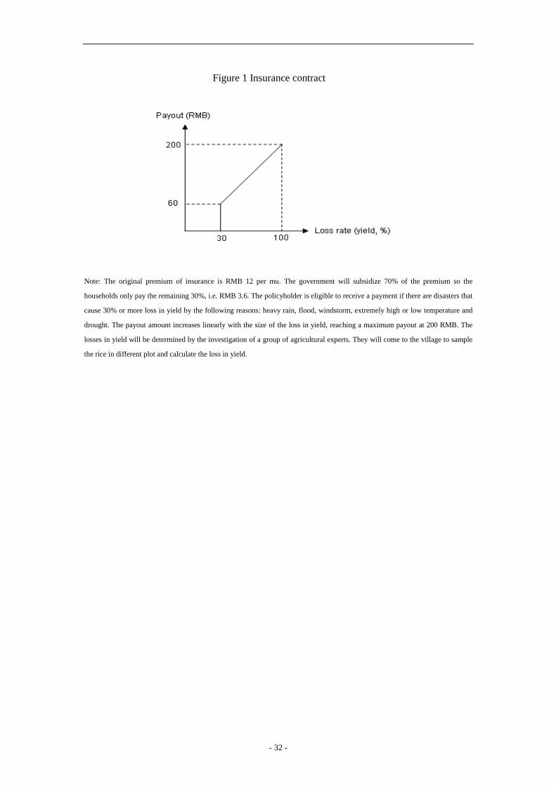
The insurance contract is depicted in figure 1.
[Insert Figure 1 Insurance contract]
The full insurance premium is 12 RMB per mu per season.10The government
subsidizes 70 percent of the premium so that the households only pay 3.6 RMB. The
policyholder is eligible to receive a payment if there are disasters that cause 30
percent or more loss in yield for one of the following reasons: heavy rain, floods,
windstorms, extremely high or low temperatures, or drought. Losses in yield are
determined by investigation by a group of insurance agents and agricultural experts.
The payout amount increases linearly with the size of the loss in yield. For example,
consider a farmer growing rice with an area of 2 mu. The normal yield per mu is
500kg but this year a wind disaster happens to reduce the yield to 300kg per mu. In
that case, since the loss in yield is 40%, the farmer is supposed to get 200*40% = 80
RMB per mu from the insurance company. Note that the insurance is partial: payout is
capped at 200 RMB, but the medium gross income in our sample is around 855 RMB
per mu so the insurance covers at most 25 percent of income.
It’s also important to note that the post-subsidy price is below the actuarially fair
price according to our calculations. The profit of the insurance company is revenue
minus payment to households and fixed cost.
FCindemnitypNpremiumN −⋅⋅−⋅=π
where p is the probability of future disasters, N is the number of households who buy
insurance and the indemnity is the payment to households when there is a disaster.
According to private communications with local government officials, the actual
probability of a disaster that leads to 30 percent or more loss is around 10 percent.
Since 60%106.3 ⋅⋅<⋅ NN , the post subsidy price is below fair price. However,
because the pre-subsidy price is higher than the fair price, the insurance company
earns a profit if its fixed costs are not large.
10 1 USD≈6.35 RMB or 3.95 RMB in PPP; 1 mu≈666.7 m2; 1 mu≈0.165 acre; Farmers produce two or three seasons of rice every year.
- 7 -
3. Experimental Design and Survey Data
3.1 Experimental Design
In 2009 and 2010, we randomly selected 16 natural villages as our experiment sites.
Nine hired enumerators consisting of government officials and primary school teachers,
together with the two authors, visited each village and conducted surveys of 885 households
before the beginning of the growing season. Randomization is conducted at the household
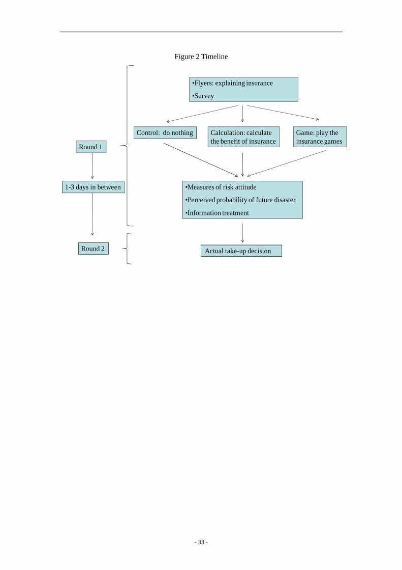
level. There were two rounds of interviews for each household. The timeline is presented in
the figure below.
[Insert Figure 2 Timeline]
We implemented the baseline survey and intervention in round 1. The procedure is as
follows: the enumerators first gave households flyers with information about the insurance
contract, including liability, period and premium. Households were then asked questions
about their socioeconomic background. If the households were assigned to the game treatment,
the enumerators played the insurance games with them (discussed below). After the games,
we elicited risk attitudes and the perceived probability of future disasters for all households
(discussed below). If the households were assigned to the information treatment (discussed
below), the enumerators informed them of the actual probability of a large disaster.11 At the
end of round 1, households were also told to think about whether they would like to buy the
rice insurance and that enumerators would come back to ask them to make a decision in round
2.
Round 2 was conducted one to three days later. In round 2, the enumerators asked
sample households to indicate their purchase decisions. The decisions would be passed to
insurance company who would collect the premium later.12
Round 2 was conducted one to three days later. In round 2, the enumerators
asked sample households to indicate their purchase decisions. The decisions would be
passed on to the insurance company, which would collect the premium later.13
11 As estimated by government officials. 12 Note that in round 1 the enumerators were randomly assigned to households while in round 2 one enumerator visited one or more villages. In our data, 22 percent of households (196 households) were visited twice by the same enumerator. 13Note that the enumerators were randomly assigned to households in round 1, while in round 2 one
- 8 -
At the end of round 1, we paid each household 5 RMB to compensate for the
participant’s time. As discussed in the introduction, we did not incentivize decisions in order
to eliminate confounding due to income effects.
We first approached the leaders of the villages and obtained a list that included the
names of villagers and basic information about them14.Then we stratified the households by
their natural villages, ages of household heads, and area of rice production. In each stratum,
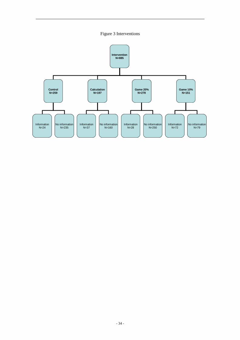
households were randomly assigned to one of eight interventions. We randomized the
treatments in two dimensions: how the contract was explained to the households (four groups)
and whether the true disaster risk was revealed to the households (two groups). Figure 3
summarizes our design with eight groups in round 1.
[Insert Figure 3 Interventions]
The contract was explained in the following four ways. In the Control group, the
enumerators gave households rice insurance flyers and went through the information about
the contract. Then household heads were asked to fill out a short survey about their age,
education, insurance experience, disasters experienced in recent years, production, social
networks, risk attitudes and perception of the probability of future disasters.
In the Calculation group, the enumerators followed the same procedure as in the control
group but additionally calculated the expected benefit of buying insurance if zero, one, two or
three disasters were to happen in the following ten years. Enumerators went through the
calculation with households and told them the summary: “According to our calculations, if
there is no large disaster in next 10 years, it is better to not buy any insurance in the following
10 year. If there is at least one relatively large disaster, it is better to always buy insurance in
the following 10 years.”
In the Game 20% (and Game 10%) groups, the enumerators followed the same
procedure as in the control group and then played the hypothetical insurance games with 20%
(or 10%) probability of disaster for ten rounds. The game was played in the following way.
Household heads were first asked whether they would hypothetically like to buy insurance in
enumerator visited one or more villages. In our data, 22 percent of households (196 households) were visited twice by the same enumerator. 14We excluded households that did not grow rice. Those were households that were raising livestock or who had abandoned the land and were looking for jobs in urban areas.
- 9 -
2011 and then played a lottery with 20% (10%) probability of a disaster. We implemented the
lottery by drawing randomly from a stack of cards; for example, in the Game 20%case, two
out of ten cards signified disaster. After the lottery results were revealed, enumerators helped
the household heads calculate the income from that year based on the expected income per
acre and insurance payments. The game was then played for another nine rounds from
hypothetical year 2012 to year 2020.15At the end of the game, we gave households the
same information as in the Calculation group. Note that the game treatment provided not
only financial education but also the second source of randomization: the number of the
hypothetical disasters experienced during the games is randomized.
In a crossed randomization, we also randomized whether households were informed at
the end of round 1 of the actual probability of disaster, which local government officials
estimate at 10%. This randomization is interacted with how the contract is explained; thus, we
have eight groups in total.
To summarize, the Calculation treatment provides households with information about
the expected benefits of insurance. The Game treatment makes households acquire
(hypothetical) disaster experience and provides households with information about the
benefits of insurance. The (crossed) Information treatment provides households with
information about the risk of disaster.
Risk attitudes and the perceived probability of future disasters were elicited for all
households. For those who were assigned to play games, the above two measures were
elicited after playing the insurance games. Comparing these measures between the game
group and the other groups allows us to test whether playing games changes these parameters
and further changes the actual insurance take-up.16Risk attitudes were elicited by asking
households to choose between increasing amounts of certain money (riskless option A) and
risky gambles (risky option B) in Appendix TableA1. We use the number of riskless options
as a measurement of risk aversion.
15The setup implies that 89 percent of households in the Game 20% group and 65 percent of the households in the Game 10% group were expected to experience at least one disaster. In our data, 82 percent of households in the Game 20% group and 66 percent of households in the Game 10% group experienced at least one disaster. 16We did not ask these questions before the games; if players had decided to act consistently with their answers, this would have obscured the treatment effects.
- 10 -
The perceived probability of future disasters was elicited by asking households “what do
you think is the probability of a disaster that leads to more than 30 percent yield loss next
year?” We used a simple mechanism to illustrate probability, which might be a difficult
concept for households with limited education.17
3.2 Survey Data
We implemented the survey in three waves. In the first wave (181 households, August
2009), we implemented only the control and Game 20%in the no information treatment. In
the second wave (379 households, early March 2010), we implemented the control, the
Calculation, and Game 20%in the no information treatment. In the third wave (325
households, late March 2010), we implemented all eight interventions. Because the Game
10% group and the information treatment were only conducted in the third wave, we
oversample the Game 10% group; the total sample sizes of the Game 10% group and the
information treatment are smaller than in the other groups.
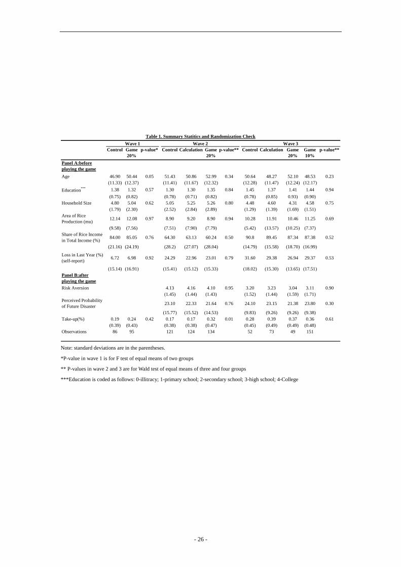
[Insert Table 1 Summary statistics]
Table 1 presents summary statistics and balance checks separately for each wave. In total,
we visited 885 households in round 1 and 816households in round 2. The overall attrition rate
between round 1 and round 2was 7.8 percent. While the attrition was slightly higher in the
game group, 9.8 percent, than in the control and calculations groups, respectively 6.2 and 5.6
percent, the difference in attrition between groups is not statistically significant. Attrition was
11.8 percent in the information group, which is not significantly different from the 10.4
percent attrition in the no information group in wave 3.
The summary statistics show that household heads are almost exclusively male. The
average education level is between primary school and secondary school. The average
individual is risk averse. The randomization check shows that most control variables are
balanced. The only exception is that in wave 1, the households in the game group are older
than those in the control group. However, the regressions in the next section show that the
17The enumerators gave sample individuals 10 small paper balls and asked them to put these paper balls into two areas: (1) no disaster reducing yield more than 30% next year and (2) disaster reducing yield more than 30% next year. If households put two paper balls into area (2) and eight paper balls into area (1), their perceived probability of future disaster is around 20%.
- 11 -
relationship between take-up and age is in any case insignificant.
4. Empirical Result
4.1 The Impact of Hypothetical Experience on Actual Take-up
In what follows, “Game” refers to households who were assigned to the Game 20%
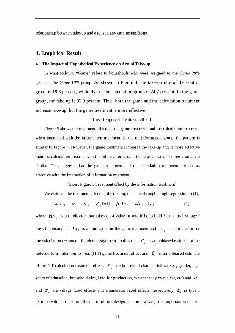
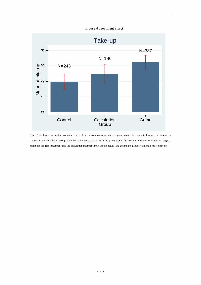
group or the Game 10% group. As shown in Figure 4, the take-up rate of the control
group is 19.8 percent, while that of the calculation group is 24.7 percent. In the game
group, the take-up is 32.3 percent. Thus, both the game and the calculation treatment
increase take-up, but the game treatment is more effective.
[Insert Figure 4 Treatment effect]
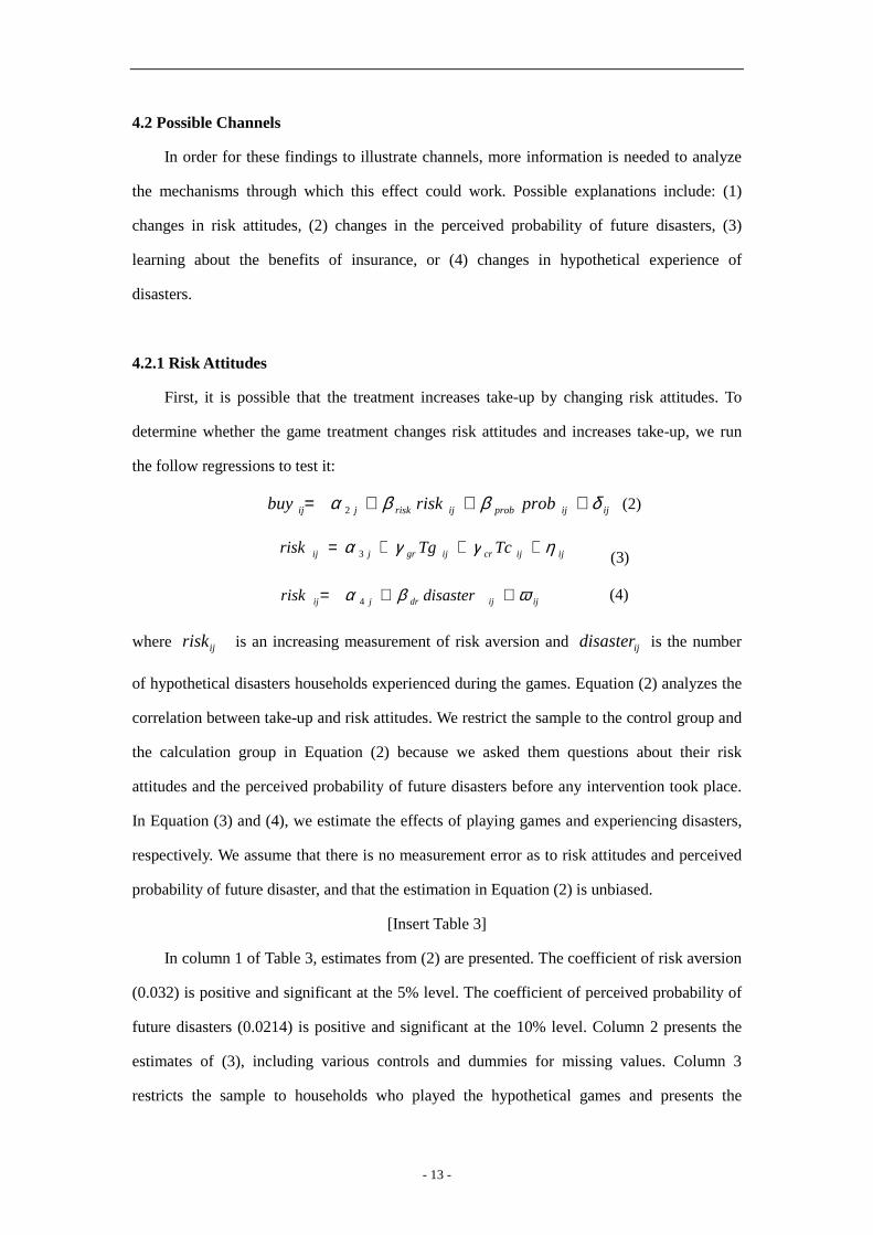
Figure 5 shows the treatment effects of the game treatment and the calculation treatment
when interacted with the information treatment. In the no information group, the pattern is
similar to Figure 4. However, the game treatment increases the take-up and is more effective
than the calculation treatment. In the information group, the take-up rates of three groups are
similar. This suggests that the game treatment and the calculation treatment are not as
effective with the interaction of information treatment.
[Insert Figure 5 Treatment effect by the information treatment]
We estimate the treatment effect on the take-up decision through a logit regression in (1):
ijijijcijgkjij XTcTgbuy εφββαα +++++= (1)
where ijbuy is an indicator that takes on a value of one if household i in natural village j
buys the insurance. ijTg is an indicator for the game treatment and ijTc is an indicator for
the calculation treatment. Random assignment implies that gβ is an unbiased estimate of the
reduced-form intention-to-treat (ITT) game treatment effect and cβ is an unbiased estimate
of the ITT calculation treatment effect. ijX are household characteristics (e.g. , gender, age,
years of education, household size, land for production, whether they own a car, etc) and jα
and kα are village fixed effects and enumerator fixed effects, respectively. ijε is type I
extreme value error term. Since our roll-out design has three waves, it is important to control

- 12 -
for potential confounding variables such as the covariates (X) and fixed effects. We report
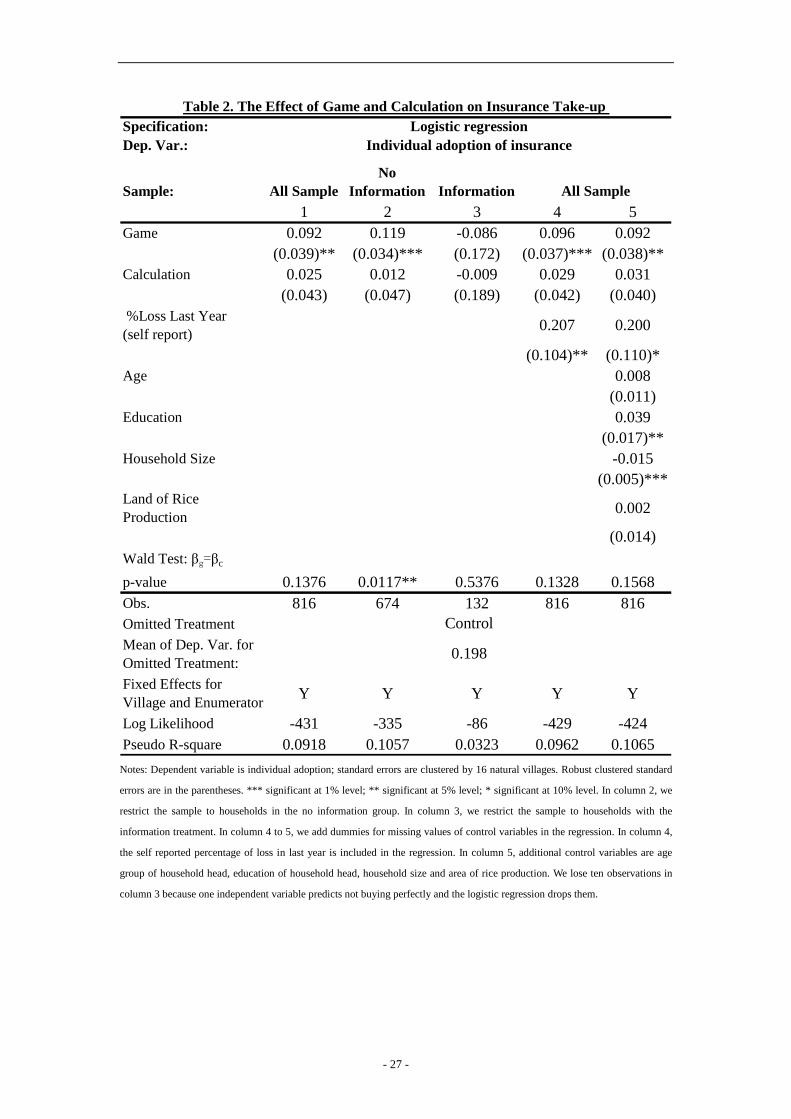
marginal effects in Table 2.
[Insert Table 2]
Column 1 presents results from the simplest possible specification, where the only right
hand side variables are the indicators for the game treatment, the calculation treatment, and
the village and enumerators fixed effects. The marginal effect of the game treatment
(0.096) is positive and significant at the 5% level. Thus, the game treatment increases the
take-up by 9.6 percentage points, which is about a 48 percent increase relative to the baseline
take-up of 20 percentage points. The marginal effect of the calculation treatment (0.027) is
positive but it is not statistically significant.
In column 2, we restrict the sample to households in the no information group. The
marginal effect of the game treatment (0.126) increases and the pattern is similar to column 1.
In column 3, we restrict the sample to households in the information group. The marginal
effects of the game and calculation treatment are imprecisely estimated; they are negative and
not statistically significant. The difference in marginal effects between the information group
and the no information group is significant at the 10% level.
In column 4, the self reported percentage of loss last year and a dummy for missing
values are included in the regression with all samples. The pattern is similar to column 1.The
marginal effect of the percentage of loss last year is 0.22%; this is significant at the 10% level.
Thus, the effect of playing games is roughly of the same magnitude as the effect of a 45
percentage point increase in actual loss last year.
In column 5, a variety of other control variables and dummies for missing values are
additionally included in the regression with all samples. The pattern is still similar to column
1.Education level is positively correlated with take-up and household size is negatively
correlated with the take-up.
In sum, the game treatment increases the insurance take-up by 9 to 10 percentage points,
resulting in an increase of around 45 to 50 percent relative to baseline take-up of 20
percentage points. The effect of playing games is roughly of the same magnitude as a 45
percentage point increase in actual loss during the previous year.
- 13 -
4.2 Possible Channels
In order for these findings to illustrate channels, more information is needed to analyze
the mechanisms through which this effect could work. Possible explanations include: (1)
changes in risk attitudes, (2) changes in the perceived probability of future disasters, (3)
learning about the benefits of insurance, or (4) changes in hypothetical experience of
disasters.
4.2.1 Risk Attitudes
First, it is possible that the treatment increases take-up by changing risk attitudes. To
determine whether the game treatment changes risk attitudes and increases take-up, we run
the follow regressions to test it:
ijijprobijriskjij probriskbuy δββα +++= 2 (2)
ijijcrijgrjij TcTgrisk ηγγα +++= 3 (3)
ijijdrjij disasterrisk ωβα ++= 4 (4)
where ijrisk is an increasing measurement of risk aversion and ijdisaster is the number
of hypothetical disasters households experienced during the games. Equation (2) analyzes the
correlation between take-up and risk attitudes. We restrict the sample to the control group and
the calculation group in Equation (2) because we asked them questions about their risk
attitudes and the perceived probability of future disasters before any intervention took place.
In Equation (3) and (4), we estimate the effects of playing games and experiencing disasters,
respectively. We assume that there is no measurement error as to risk attitudes and perceived
probability of future disaster, and that the estimation in Equation (2) is unbiased.
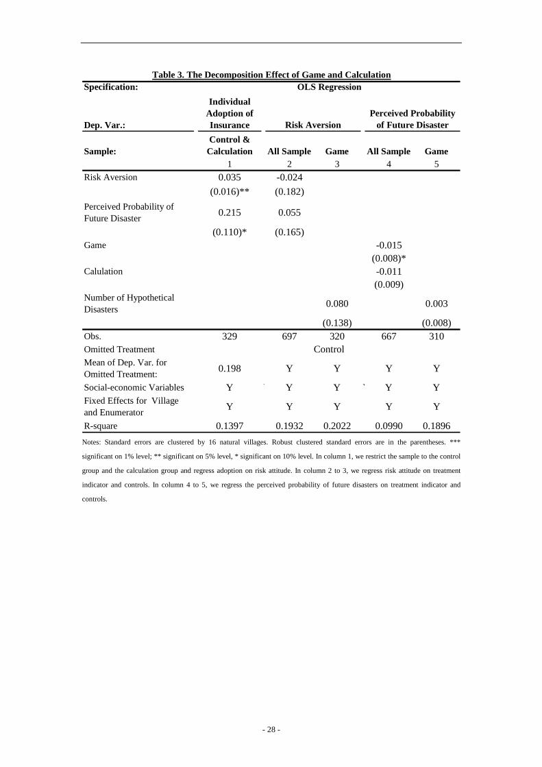
[Insert Table 3]
In column 1 of Table 3, estimates from (2) are presented. The coefficient of risk aversion
(0.032) is positive and significant at the 5% level. The coefficient of perceived probability of
future disasters (0.0214) is positive and significant at the 10% level. Column 2 presents the
estimates of (3), including various controls and dummies for missing values. Column 3
restricts the sample to households who played the hypothetical games and presents the

- 14 -
estimates of (4). The results show that the treatment has no effect on risk aversion and the
coefficient of the number of hypothetical disasters is not statistically significant.
To determine whether the game treatment changes risk attitudes and increases take-up,
we stack Equation (1), (2), and (3), generate indicators for each equation, and estimate the
regression system. To account for the correlation of error terms between each equation,
standard errors are clustered by 16 natural villages. We test the hypothesis: ggrrisk βγβ = .
We reject the hypothesis at the 5% level (p=0.039), with the 95% confidence interval ranging
in [-0.013, 0.011]. To determine whether the number of hypothetical disasters changes risk
attitudes and increases take-up, we stack Equation (1), (2), and (4) and estimate the regression
system. We test the hypothesis: ggrdr βγβ =48.1 , where 1.48 is average number of
hypothetical disasters experienced during the games. We reject the hypothesis at the 5% level
(p=0.044), with the 95% confidence interval of grdrγβ48.1 ranging in [-0.004, 0.004].
These results suggest that changes in our measurement of risk attitudes are unlikely to explain
our main treatment effect.
4.2.2 The Perceived Probability of Future Disaster
Demand for insurance also depends on the perceived probability of future disasters. It is
possible that the games increase take-up by changing the perceived probability of future
disasters. To test this channel, we run the following regressions:
ijijcpijgpjij TcTgprob ηγγα +++= 3 (5)
ijijdpjij disasterprob ωβα ++= 4 (6)
where ijprob is the perceived probability of future disaster. In Equation (5) and (6), we
estimate the effects of playing games and experiencing disasters, respectively. The results of
(5) and (6) are presented in column 4 and 5 in Table 3, respectively.
The treatment has a negative effect on the perceived probability of future disasters in
columns 4. The coefficient of the number of hypothetical disasters is not significant.
Following a similar procedure as in section 4.2.1, we test the hypothesis ggpprob βγβ = and
- 15 -
ggpdp βγβ =48.1 to determine whether changes in the perceived probability of future
disasters is the channel. We reject that at the 5% level.
To determine whether the total effects of changing risk attitudes and the perceived
probability of future disasters are the channel through which the observed effects operate, we
follow a similar procedure as in section 4.2.1 and test the following two hypothesis:
ggpprobgrrisk βγβγβ =+ and ggpdpgrdr βγβγβ =+ 48.148.1 .We reject the hypothesis at
the 5% level. These results suggest that the total effects of changes in risk attitudes and the
perceived probability of future disasters are unlikely to explain our main treatment effect.
4.2.3 Learning the Benefits of Insurance
It is also possible that playing insurance games provides direct information about the
benefits of insurance. To test that, we compare the treatment effect of the game and
calculation treatment; the difference between those two interventions should indicate whether
households acquire disaster experiences during the games.
We run various regressions with (1) and report the p-value of Ward test cg ββ = in
Table 2. In columns 1, 4 and 5, we use the whole sample. The difference between gβ and
cβ is around 7 percentage points and it is not statistically significant (p-value of Ward test is
between 0.13 and 0.16). In columns 2, we restrict the sample to the no information group. The
difference between gβ and cβ is around 11 percentage points and is significant at the 5%
level.
In sum, when we consider the channel of the game treatment effect without the
interaction effect of the information treatment, we conclude that learning about the benefits of
insurance is unlikely to explain the treatment effect of playing games. When we consider the
channel of the game treatment effect and interaction effect of the information treatment, there
is suggestive evidence that learning about the benefit is unlikely to explain the game
treatment effect.
4.2.4 The Experience of Hypothetical Disasters
- 16 -
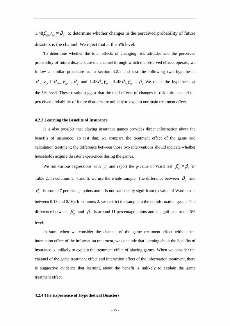
Another hypothesis is that hypothetical experience matters. To test this hypothesis, we
explore the randomization of the number of hypothetical disasters during the game. We
present Figure 6 about actual take-up and the hypothetical disasters experienced during the
games.
[Insert Figure 6]
In the Game 20% group, the take-up among households who experienced two or more
disasters is higher than that among those who experienced zero or one disaster. In the Game
10% group, the take-up of households who experienced one disaster is higher than those who
experienced either zero or two and more disasters. However, given the relatively large
standard deviation, Figure 6 provides only suggestive evidence that the take-up rate is
increasing in the number of hypothetical disasters experienced and that the take-up in the
group with no hypothetical disasters is greater than that in the control group.
To understand this further, we run the following regression:
ijijdisasterjij disasterbuy δβα ++= (7)
where ijdisaster is the number of hypothetical disasters experienced during the games.
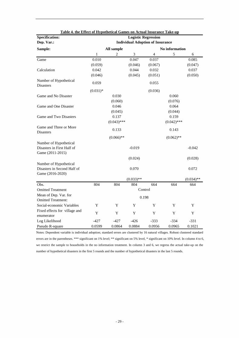
[Insert Table 4]
The marginal effect estimated in (7) is presented in column 1 and 4 of Table 4. In column
1, the coefficient (0.059) is positive and statistically significant at the 10% level. In the no
information group (column 4), the coefficient (0.055) is positive but not significant (p=0.127).
Therefore, the results suggest that the treatment effects were driven mainly by those who
experienced more hypothetical disasters during the games.
Hypothetical experience might change two things: understanding about insurance and
vividness. We run regression in Equation (8) to analyze these two effects:
ijijijijijjij disasterdisasterdisasterdisasterbuy εββββα +++++= 3210 3210(8)
where ijdisasterK is an indicator that takes on a value of one if households experience K
disasters during the games. 0β captures the understanding effect; the difference
between 0β and other coefficients captures the vividness effect.
The marginal effect of (8) is presented in column 2 and 5 in Table 4. The coefficients of

- 17 -
ijdisaster0 and ijdisaster1 are positive but not statistically significant. Indicators for more
disasters are positive, statistically significant and relatively large in magnitude. In the no
information group (column 4), the coefficients are relatively larger, which is similar to what
we have seen in Table 2. The difference between 1β and 2β is statistically significant at the
10% level. However, we cannot reject the hypothesis that 0β and 1β are the same.
Therefore, we cannot distinguish between the understanding effect and the vividness effect.
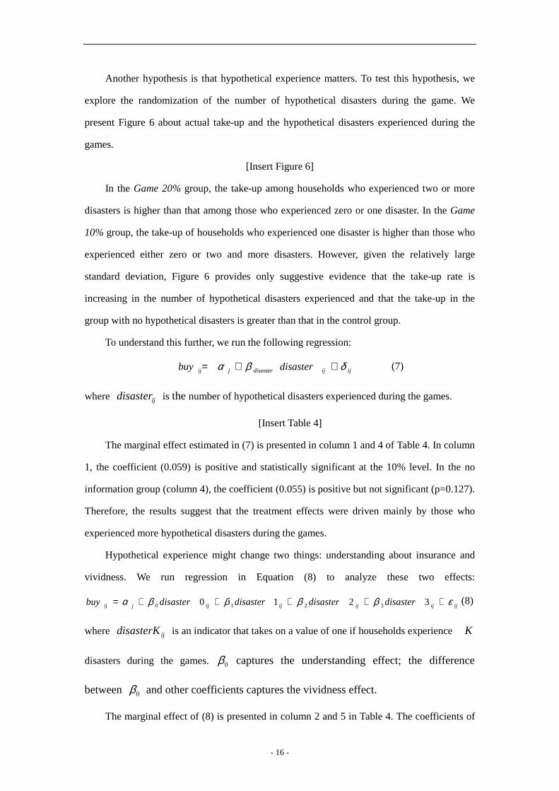
To further understand how hypothetical experience influences take-up, we present the
take-up conditioning on disaster in the first 5 rounds and in the last 5 rounds in Figure 7.
[Insert Figure 7]
The evidence in Figure 7 suggests that the number of hypothetical disasters experienced in the
first 5 rounds does not influence take-up, whereas the number of disasters in the last 5 rounds
appears to have a bigger effect.
We then create two new variables: the number of hypothetical disasters in the first 5
rounds and the number of hypothetical disasters in the last 5 rounds. We run the following
regression:
ijijlijfjij lastdisasterfirstdisasterbuy δββα +++= 5_5_ 55 (9)
As seen in column 4, the coefficient of “disasters in the first half” is negative and not
statistically significant. However, the coefficient of “disasters in the last half” is positive and
significant at the 5% level. The coefficient suggests that experiencing an additional disaster in
the last half increases take-up by 7.0 percentage points. In the no information group (column
6), the coefficient of the last 5 rounds is also positive and significant at the 5% level. This
pattern is robust to different measurement of the first and last few rounds. If we regress
take-up on the number of hypothetical disasters in the first (10-n) rounds and that in the last n
rounds, we find that when n equals 5,6,7,8 or 9, the coefficients of the last n rounds are
positive and significant at the 5% level.18 These results are consistent with the literature in
experienced utility and recency effects (Fredrickson and Kahneman 1993; Schreiber and
Kahneman, D. 2000), where they find that the affect experienced during the last moments of
18 See Appendix Table A4 for detail
- 18 -
the experiment has a privileged role in subsequent evaluations, and late moments in the
experiment are assigned greater weight than earlier ones.
To summarize, we find that both the total number of disasters and the number of
disasters in last few rounds increase take-up significantly. These results suggest that the
experience of recent hypothetical disasters might be the channel through which the games
influence insurance decisions.
5. Models
The evidence so far implies that hypothetical experience influences the actual insurance
decisions. In this section, we present a simple model to illustrate how such an effect could
occur. In section 5.1, we show that standard constant absolute risk aversion (CARA)
preferences and constant relative risk aversion (CRRA) preferences are unlikely to explain the
data. In section 5.2, we add a weight parameter to the utility function to capture the influence
of experience. Then we estimate the parameters through a maximum likelihood method
(MLE).
5.1 Standard Model
We first consider a simple model with CARA preferences commonly used in the
insurance literature (Einav et al. 2010).
αα )exp(
)(x
xu−−=
(11)
With CARA preferences, the consumer’s wealth does not affect his insurance choices.
Therefore, the take-up decisions should be determined by the joint distribution of risk
attitudes and perceived probability of future disasters.
Let )(aU denote the household utility as a function of the insurance decision. 1=a
if the household buys the insurance and 0=a if the household does not buy the insurance.
Let ),( τb denote the insurance contract in which b is the repayment of insurance if there
is a disaster and τ is the premium. Let x be the gross income of rice production and p
the perceived probability of future disasters. Let l denote the loss in yield. The expected
- 19 -
utility of not buying the insurance is:
)(p)(p)-(1)0( lxuxuaU −+== (12)
If a household buys insurance, it should earn its normal income and pay the premium
when there is no disaster; it should have a loss and receive payment from the insurance
company when there is a disaster. The utility of buying the insurance is:
)(p)(p)-(1)1( blxuxuaU +−−+−== ττ (13)
The condition for the household to buy the insurance is
)0()1( =>== aUaU (14)
It is straightforward to show that the households who are more risk averse and whose
perceived probabilities of future disasters are larger are more likely to buy the insurance.
To test whether the standard CARA preferences could explain our data, one way is to use
the parameter as measured, calibrate individual decisions and compare the calibrated
decisions with actual decisions. We assume that there is no measurement error for risk
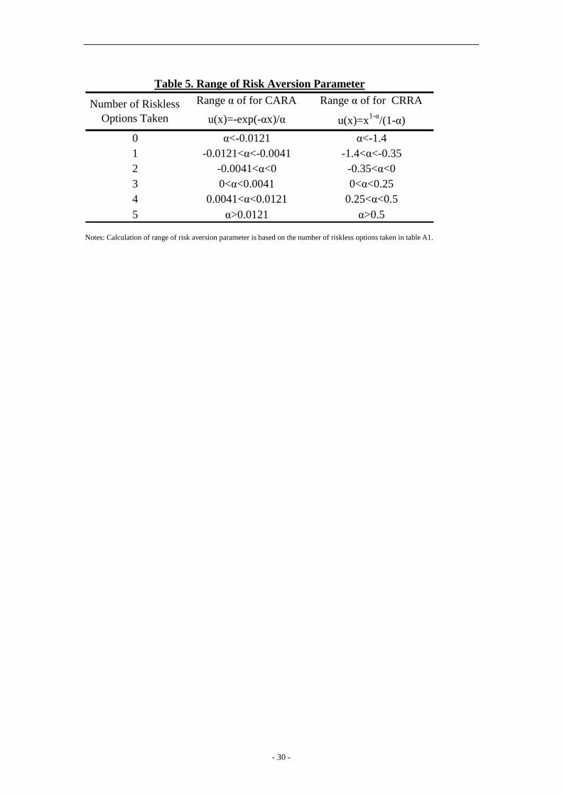
aversion (α ) or for the perceived probability of future disasters (p). Although we do not
observe parameter α , we can make use of the choices in Table 1 to estimate the intervals of
their α in the utility function. The intervals of α under CARA and CRRA are presented in
Table 5. If a household takes two riskless options, α should be greater than zero and less
than 0.0041 under CARA preferences. The details of the simulation procedures are discussed
in Appendix A.
[Insert Table 5]
We find that the mean of simulated take-up is 81.08% and the standard deviation is
0.0049. This contradicts our actual data that the take-up in the sample is 26.84%. This
suggests that standard CARA and CRRA preferences are unlikely to explain our data.
Another route is to ignore α and p as elicited. Suppose that we had not elicited
measures for risk aversion and perceived probability of future disasters. Then we estimate
α and p in the logit formula (15) through MLE:
))0(exp())1(exp(
))1(exp()1(
=+====
aUaU
aUaP (15)
We find that the model is not identifiable. The log-likelihood function reaches a flat
region and the combination of α and p falls into the following two categories: (1) negative
- 20 -
α (risk seeking) and p greater 17% (2) positive α (risk averse) and p less than 5%.
This contradicts our data that average risk attitude implies risk aversion and that the average
perceived probability of future disasters is around 20%.
In sum, both the calibrated decisions and the estimated parameters contradict our data
under standard CARA and CRRA preferences. These results suggest that standard CARA and
CRRA preferences are unlikely to explain the observed take-up rates in the presence of the
perceived probability of future disasters which our questions elicited.
5.2 Model Based on Experience
We have shown that standard CARA and CRRA preferences are unlikely to explain the
data. In order to develop a model that fits our data, we add a weight parameter to capture the
effect of experience. It is possible that households buy more insurance because they pay more
attention to disasters and benefits after they experience the hypothetical disasters during the
games. We develop a simple model in the following.
)(p)(p)-(1)0( lxuxuaU µ−+== (16)
)(p)(p)-(1)1( blxuxuaU µµττ +−−+−== (17)
where µ is a parameter that measures the weight of disaster loss and insurance benefits. The
idea is that households might give less weight to disasters and benefits which they experience
infrequently. When they are treated with games, they experience disasters and insurance
benefits during the hypothetical games. These hypothetical disasters draw their attention to
disaster loss and insurance benefits and increase the weight parameter µ .
It is straightforward to show that, under the assumption of CARA preferences with
inattention parameter µ , if 0>α , then 0)1( >∂==∂
µbuyP . To the extent that playing games
increases µ , it would increase the insurance take-up. To test this, we allow µ in the group
who do not play games (1µ ) to be different from µ in the group who play games (2µ ).
Then we estimate 1µ and 2µ with MLE and simulation. The details of the estimation
procedures are discussed in Appendix A.
[Insert Table 6]
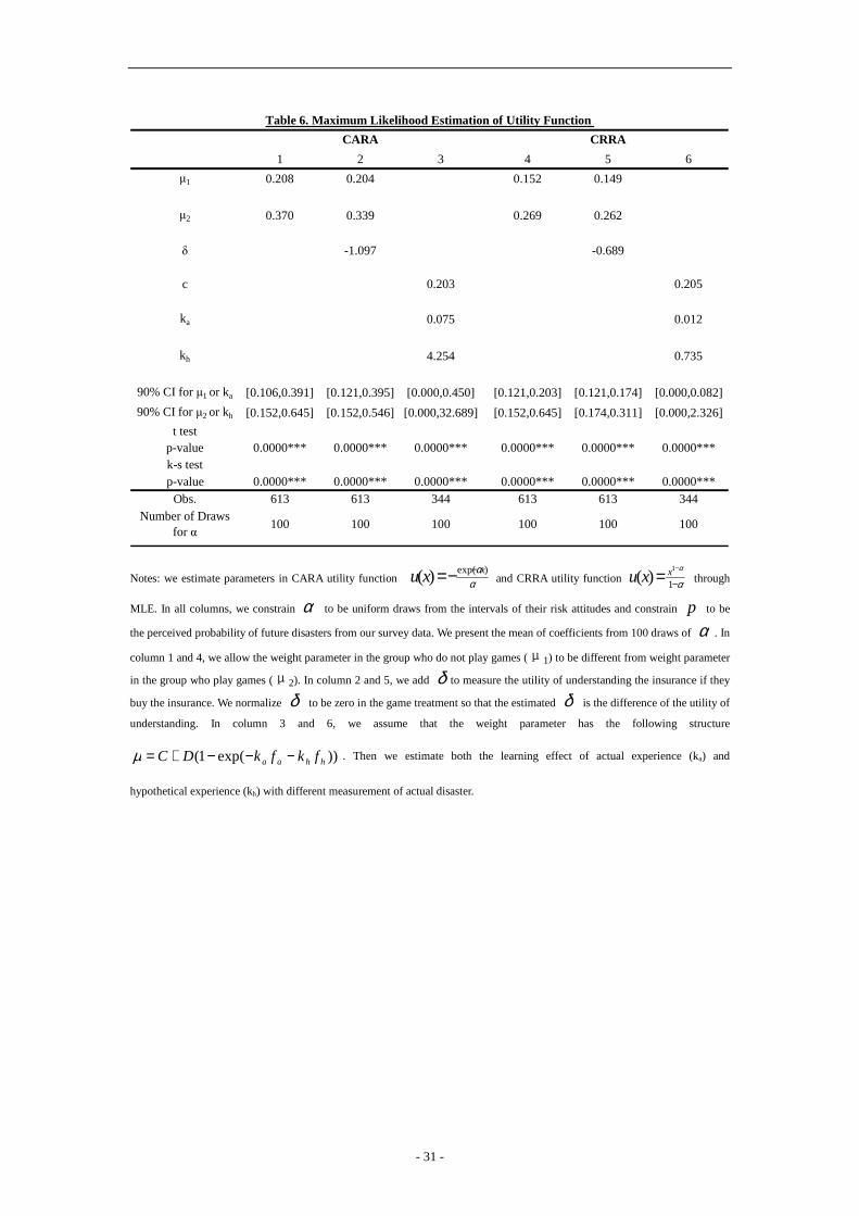
The result is presented in column 2 table 6. We find that the estimated mean of 1µ is

- 21 -
around 0.21 and that 2µ is around 0.37. The T-test and Kolmogorov-Smirnov test show that
the mean and the distribution are significantly different at the 1% level. Column 6 presents the
result with CRRA preferences. Although the point estimates are different, the key pattern is
similar. These results are consistent with our hypothesis that playing games increases µ and
thus increases insurance take-up.
Hypothetical experience might have two effects: changes in understanding and changes
in vividness. We add another parameter δ in (17):
δµµττ ++−−+−== )(p)(p)-(1)1( blxuxuaU (18)
where δ measures the utility of understanding insurance if they buy the insurance. The
intuition is that households would be less happy if they buy something they do not understand
than something they understand. It might capture ambiguity aversion and it is a reduced form
in our model. We normalize δ to be zero in the game treatment so that the estimated δ is
the difference of the utility of understanding. We estimate 1µ , 2µ and δ with the same
procedure to estimate 1µ and 2µ . The results are presented in column 3.
The estimated mean of 1µ is about 20.4% and 2µ is about 33.9%. The T-test and
Kolmogorov-Smirnov test show that the mean and the distribution are significantly different
at the 1% level. The estimated mean of δ is -1.097 and the t-test shows that the mean is
significantly different from zero at the 1% level. Since we normalize δ to be zero in the
game treatment, this means that the utility of understanding is higher in the game treatment.
Column 7 presents the result with CRRA preference. Although the point estimates are
different, the key pattern is similar. These results are consistent with our hypothesis that
playing games increases the understanding and vividness and thus increases the insurance
take-up.
In order to understand the empirical relationship between experience and the weight
parameter, we modelµ following the lead of Agarwal et al. (2011).
))exp(1( hhaa fkfkDC −−−+=µ
where 0,,, >DCkk ha , and 1≤+ DC .
- 22 -
af is actual experience, measured by percentage of disasters reducing yield more than
30% in the past 3, 2 or 1 years. hf is hypothetical experience, measured by percentage of
disasters during 10 rounds of games. ak and hk capture the rate of learning from actual
experience and hypothetical experience. With enough experiences, attention saturates to C +
D. If 1=+ DC , attention is perfect in the long run, but if 1<+ DC , attention is imperfect,
even in the long run. Here, we assume 1=+ DC . Then we could estimate ak and hk
and compare the effect of actual and hypothetical experience.
In column 4, we estimate the learning effect of both actual experience (ka) and
hypothetical experience (kh) under CARA preferences. af is measured by percentage of
disasters reducing yield more than 30% in the past 3 years. The mean of ka is 0.075 and the
mean of kh is 4.254; they are significantly different at the 1% level. Column 8 presents the
result with CRRA preferences. Although the point estimates are different, the key pattern is
similar. These results suggest that both actual and hypothetical experience matter. Moreover,
experience acquired in the recent insurance game has a stronger effect on the actual insurance
take-up than that of real disasters in the previous year.
6. Conclusion
It is important to understand why the take-up for weather insurance is low even when
farmers face substantial natural risks. We apply a novel method of financial education and
test for the role of experience and information in weather insurance take-up in rural China.
We find that playing insurance games increases the actual insurance take-up by 9.6 percentage
points, a 48% increase relative to the baseline take-up of 20 percentage points. We investigate
the possible mechanisms through which this effect could work, and find that changes in
experience of disasters and insurance benefits are very likely to be the channel.
There is mixed evidence in the literature as to whether financial education is effective to
change individual decisions. Why is financial education effective sometimes but not others?
Under what circumstances is financial education effective? This paper shows that financial
education with simulated experiences can help increase insurance take-up in rural areas.

- 23 -
Gaurav et al. (2011) finds similar results in India. Song (2011) finds that learning the concept
of compound interest has a positive and significant effect on weather insurance adoption in
rural China. These suggest that we should first identify the barriers to individual participation
and then apply specific financial education to remove the barriers. This seems to work better
than general financial education.
From a policy perspective, this paper suggests that policy makers should take into
account the individuals’ biases when design policies, especially in rural areas where most
people are less educated. In particular, policy makers can provide cheap financial education to
overcome individual constraints and thus improve individual welfares.
From a methodological standpoint, this paper is among the first to use a laboratory
experiment as an intervention in the field experiment.19 We find that the laboratory
experiment influenced the field behavior in our setting. By using laboratory experiments,
researchers can explicitly manipulate more variables which are endogenous or are otherwise
difficult to manipulate. For example, Malmendier and Nagel (2010) find that individuals who
have experienced low stock-market returns throughout their lives so far are less likely to
participate in the stock market. However, it is difficult to manipulate experience in order to
influence individual decisions. In this paper, we use a laboratory experiment to simulate
experiences and influence field behaviors. We hope to explore in future research whether this
can apply to other settings.
References
Agarwal, Sumit, John C Driscoll, Xavier Gabaix, and David Laibson (2011), “Learning in the
Credit Card Market”, Available at SSRN: http://ssrn.com/abstract=1091623
Ashraf, Nava, Dean Karlan, and Wesley Yin (2006), “Tying Odysseus to the Mast: Evidence
from a Commitment Savings Product in the Philippines”, Quarterly Journal of
Economics, 121(2), pp. 635-672
Banerjee, Abhijit V. and Sendhil Mullainathan (2008), “Limited Attention and Income
Distribution”, American Economic Review: Papers & Proceedings 2008, 98:2, 489–493
Cai, Jing (2011). “Social Networks and the Decision to Insure: Evidence from Randomized
Experiments in China”, Working Paper, University of California at Berkeley.
Carlin, B. I. and Robinson, D. T. (2011), “What does financial literacy training teach us?”
National Bureau of Economic Research Working Paper Series No. 16271.
19As far as we know, the method is similar to Carter et al. (2008) and Gauravet al.(2011).
- 24 -
Carter, Michael R., Christopher B. Barrett, Stephen Boucher, Sommarat Chantarat, Francisco
Galarza, John McPeak, Andrew Mude, and Carolina Trivelli (2008), “Insuring the Never
Before Insured: Explaining Index Insurance Through Financial Education Games”. Link:
http://i4.ucdavis.edu/files/briefs/2008-07-insuring-the-never-before-insured.pdf
Choi, J., D. Laibson, B. Madrian, and A. Metrick. (2009), “Reinforcement Learning and
Savings Behavior”, The Journal of Finance 64(6), December, 2515-2534.
Cole, Shawn Allen, Gine, Xavier, Tobacman, Jeremy Bruce, Topalova, Petia B., Townsend,
Robert M. and Vickery, James I., “Barriers to Household Risk Management: Evidence
from India” (March 2011). Harvard Business School Finance Working Paper No. 09-116;
FRB of New York Staff Report No. 373.
Cole, Shawn Allen, Sampson, Thomas and Zia, Bilal (2010), “Prices or Knowledge? What
Drives Demand for Financial Services in Emerging Markets?” Journal of Finance,
Forthcoming; Harvard Business School Finance Working Paper No. 09-117.
Duflo, Esther, Michael Kremer and Jonathan Robinson (2009), “Nudging Farmers to Use
Fertilizer: Evidence from Kenya,” forthcoming, American Economic Review
Duflo, Esther and Emmanuel Saez (2003), "The Role of Information and Social Interactions
in Retirement Plan Decisions: Evidence from A Randomized Experiment," Quarterly
Journal of Economics, 2003, v118 (3, Aug), 815-842.
Fehr, Ernst and Lorenz Goette (2007), “Do Workers Work More if Wages Are High? Evidence
from a Randomized Field Experiment”, the American Economic Review, Vol. 97, No. 1
(Mar., 2007), pp. 298-317
Fredrickson, B. L., and Kahneman, D. (1993), “Duration neglect in retrospective evaluations
of affective episodes,” Journal of Personality and Social Psychology, 65, 45–55.
Gaurav, Sarthak, Shawn Cole and Jeremy Tobacman (2010), “The Randomized Evaluation of
Financial Literacy on Rainfall Insurance Take-up in Gujarat”, ILO Microinsurance
Innovation Facility Research Paper No.1,2010
Gazzale, Robert, Julian Jamison, Alexander Karlan and Dean Karlan (2009), “Ambiguous
Solicitation: Ambiguous Prescription”, Williams College Economics Department
Working Paper No. 2009-02. Available at SSRN: http://ssrn.com/abstract=1371645
Gerardi, Kristopher, Lorenz Goette and Stephan Meier (2010), “Financial Literacy and
Subprime Mortgage Delinquency: Evidence from a Survey Matched to Administrative
Data,” Social Science Research Network
Gine X., Townsend R., Vickery J. (2008), “Patterns of Rainfall Insurance Participation in
Rural India”, The World Bank Economic Review 2008;22(3):539
Ginè, X. and D. Yang (2009), “Insurance, credit, and technology adoption: Field experimental
evidence from Malawi”, Journal of Development Economics, 89, pp. 1-11
Haselhuhn, Michael P., Devin G. Pope, Maurice E. Schweitzer (2009), “Size Matters (and so
Does Experience): How Personal Experience with a Fine Influences Behavior”,
Available at SSRN: http://ssrn.com/abstract=1270746
Holt, Charles A. Markets (2005), “Games, and Strategic Behavior: Recipes for Interactive
Learning.” Unpublished Manuscript
Jensen, Robert (2000), “Agricultural Volatility and Investments in Children”, the American
Economic Review; May 2000; 90, 2; ABI/INFORM Global, pg 399.
Levitt, Steven D. and John A List (2007), “What Do Laboratory Experiments Tell Us About
- 25 -
the Real World?” Journal of Economic Perspectives 21(2):153-74.
Lusardi, A., and O. S. Mitchell (2007), "Baby Boomer Retirement Security: The Roles of
Planning, Financial Literacy, and Housing Wealth," Journal of Monetary Economics,
54:1, pp.205-24.
Lusardi, A., and P. Tufano (2008), “Debt Literacy, Financial Experiences and
Overindebtedness,” Working Paper 14808, National Bureau of Economic Research
(NBER), Cambridge, MA.
Lybbert, T.J., C.B. Barrett, S. Boucher, M.R. Carter, S. Chantarat, F. Galarza, J. G. McPeak
and A.G. Mude. (2009), “Dynamic Field Experiments in Development Economics: Risk
Valuation in Kenya, Morocco and Peru,” Agricultural and Resource Economics
Review 39(2): 176-192 (2010)
Malmendier, U. and Nagel, S. (2011), “Depression Babies: Do Macroeconomic Experiences
Affect Risk Taking?” Quarterly Journal of Economics, 126 (2011), 373–416.
Malmendier, U. and Nagel, S. (2011), “Learning from Inflation Experiences”, Working paper
Meier, Stephan, and Charles Sprenger (2008), “Discounting Financial Literacy: Time
Preferences and Participation in Financial Education Programs,” Unpublished
Plott, Charles R. (2001), Public Economics, Political Processes and Policy Applications.
Collected Papers on the Experimental Foundations of Economics and Political Science.
Volume One. Cheltenham, UK: Edward Elgar Publishing.
Rosenzweig, Mark R. and Wolpin, Kenneth I. (1993), “Credit Market Constraints,
Consumption Smoothing, and the Accumulation of Durable Production Assets in
Low-income Countries: Investments in Bullocks in India”, the Journal of Political
Economy, Vol. 101, No. 2 (Apr., 1993), pp. 223-244
Schreiber, C. A., and Kahneman, D. (2000), “Determinants of the remembered utility of
aversive sounds,” Journal of Experimental Psychology: General, 129, 27– 42.
Song, Changcheng (2011), “Neglect of Compound Interest and Pension Contributions in
China,” Working Paper, University of California at Berkeley
Stango, Victor, and Jonathan Zinmam (2009), “Exponential Growth Bias and Household
Finance,” The Journal of Finance, Volume 64, Issue 6, pages 2807–2849, December
2009
Thaler, Richard H.and Cass R. Sunstein. (2003), “Libertarian Paternalism.” American
Economic Review, Papers and Proceedings 93, no. 2 (May): 175–79.
— and (2008), “Nudge: Improving Decisions about Health, Wealth, and Happiness, Yale
University Press.
- 26 -
Control Game20%
p-value* Control Calculation Game20%
p-value** Control Calculation Game20%
Game10%
p-value**
Panel A:beforeplaying the game
Age 46.90 50.44 0.05 51.43 50.86 52.99 0.34 50.64 48.27 52.10 48.53 0.23(11.33) (12.37) (11.41) (11.67) (12.32) (12.28) (11.47) (12.24) (12.17)
Education*** 1.38 1.32 0.57 1.30 1.30 1.35 0.84 1.45 1.37 1.41 1.44 0.94
(0.75) (0.82) (0.78) (0.71) (0.82) (0.78) (0.85) 0.93) (0.90)Household Size 4.80 5.04 0.62 5.05 5.25 5.26 0.80 4.48 4.60 4.31 4.58 0.75
(1.79) (2.30) (2.52) (2.84) (2.89) (1.29) (1.39) (1.69) (1.51)Area of RiceProduction (mu)
12.14 12.08 0.97 8.90 9.20 8.90 0.94 10.28 11.91 10.46 11.25 0.69
(9.58) (7.56) (7.51) (7.90) (7.79) (5.42) (13.57) (10.25) (7.37)Share of Rice Incomein Total Income (%)
84.00 85.05 0.76 64.30 63.13 60.24 0.50 90.8 89.45 87.34 87.38 0.52
(21.16) (24.19) (28.2) (27.07) (28.04) (14.79) (15.58) (18.70) (16.99)
Loss in Last Year (%)(self-report)
6.72 6.98 0.92 24.29 22.96 23.01 0.79 31.60 29.38 26.94 29.37 0.53
(15.14) (16.91) (15.41) (15.12) (15.33) (18.02) (15.30) (13.65) (17.51)Panel B:afterplaying the game
Risk Aversion 4.13 4.16 4.10 0.95 3.20 3.23 3.04 3.11 0.90(1.45) (1.44) (1.43) (1.52) (1.44) (1.59) (1.71)
Perceived Probabilityof Future Disaster
23.10 22.33 21.64 0.76 24.10 23.15 21.38 23.80 0.30
(15.77) (15.52) (14.53) (9.83) (9.26) (9.26) (9.38)Take-up(%) 0.19 0.24 0.42 0.17 0.17 0.32 0.01 0.28 0.39 0.37 0.36 0.61
(0.39) (0.43) (0.38) (0.38) (0.47) (0.45) (0.49) (0.49) (0.48)Observations 86 95 121 124 134 52 73 49 151
Table 1. Summary Statitics and Randomization Check
Wave 1 Wave 2 Wave 3
Note: standard deviations are in the parentheses.
*P-value in wave 1 is for F test of equal means of two groups
** P-values in wave 2 and 3 are for Wald test of equal means of three and four groups
***Education is coded as follows: 0-illitracy; 1-primary school; 2-secondary school; 3-high school; 4-College
- 27 -
Specification:Dep. Var.:
Sample: All SampleNo
Information Information1 2 3 4 5
Game 0.092 0.119 -0.086 0.096 0.092(0.039)** (0.034)*** (0.172) (0.037)*** (0.038)**
Calculation 0.025 0.012 -0.009 0.029 0.031(0.043) (0.047) (0.189) (0.042) (0.040)
%Loss Last Year(self report)
0.207 0.200
(0.104)** (0.110)*Age 0.008
(0.011)Education 0.039
(0.017)**Household Size -0.015
(0.005)***Land of RiceProduction
0.002
(0.014)Wald Test: β
g=βc
p-value 0.1376 0.0117** 0.5376 0.1328 0.1568Obs. 816 674 132 816 816Omitted Treatment
Mean of Dep. Var. forOmitted Treatment:
Fixed Effects forVillage and Enumerator
Y Y Y Y Y
Log Likelihood -431 -335 -86 -429 -424Pseudo R-square 0.0918 0.1057 0.0323 0.0962 0.1065
Individual adoption of insuranceLogistic regression
Table 2. The Effect of Game and Calculation on Insurance Take-up
All Sample
0.198
Control
Notes: Dependent variable is individual adoption; standard errors are clustered by 16 natural villages. Robust clustered standard
errors are in the parentheses. *** significant at 1% level; ** significant at 5% level; * significant at 10% level. In column 2, we
restrict the sample to households in the no information group. In column 3, we restrict the sample to households with the
information treatment. In column 4 to 5, we add dummies for missing values of control variables in the regression. In column 4,
the self reported percentage of loss in last year is included in the regression. In column 5, additional control variables are age
group of household head, education of household head, household size and area of rice production. We lose ten observations in
column 3 because one independent variable predicts not buying perfectly and the logistic regression drops them.
- 28 -
Specification:
Dep. Var.:
IndividualAdoption ofInsurance
Sample:Control &
Calculation All Sample Game All Sample Game1 2 3 4 5
Risk Aversion 0.035 -0.024
(0.016)** (0.182)
Perceived Probability ofFuture Disaster
0.215 0.055
(0.110)* (0.165)Game -0.015
(0.008)*Calulation -0.011
(0.009)Number of HypotheticalDisasters
0.080 0.003
(0.138) (0.008)Obs. 329 697 320 667 310Omitted Treatment
Mean of Dep. Var. forOmitted Treatment:
0.198 Y Y Y Y
Social-economic Variables Y Y Y Y Y Y YFixed Effects for Villageand Enumerator
Y Y Y Y Y
R-square 0.1397 0.1932 0.2022 0.0990 0.1896
Control
Risk AversionPerceived Probability
of Future Disaster
Table 3. The Decomposition Effect of Game and CalculationOLS Regression
Notes: Standard errors are clustered by 16 natural villages. Robust clustered standard errors are in the parentheses. ***
significant on 1% level; ** significant on 5% level, * significant on 10% level. In column 1, we restrict the sample to the control
group and the calculation group and regress adoption on risk attitude. In column 2 to 3, we regress risk attitude on treatment
indicator and controls. In column 4 to 5, we regress the perceived probability of future disasters on treatment indicator and
controls.
- 29 -
Specification:Dep. Var.:
Sample:1 2 3 4 5 6
Game 0.010 0.047 0.037 0.085(0.059) (0.046) (0.067) (0.047)
Calculation 0.042 0.044 0.032 0.037(0.046) (0.045) (0.051) (0.050)
Number of HypotheticalDisasters
0.059 0.055
(0.031)* (0.036)Game and No Disaster 0.030 0.060
(0.060) (0.076)Game and One Disaster 0.046 0.064
(0.045) (0.044)Game and Two Disasters 0.137 0.159
(0.043)*** (0.042)***Game and Three or MoreDisasters
0.133 0.143
(0.066)** (0.062)**
Number of HypotheticalDisasters in First Half ofGame (2011-2015)
-0.019 -0.042
(0.024) (0.028)
Number of HypotheticalDisasters in Second Half ofGame (2016-2020)
0.070 0.072
(0.033)** (0.034)**Obs. 804 804 804 664 664 664Omitted TreatmentMean of Dep. Var. forOmitted Treatment:Social-economic Variables Y Y Y Y Y YFixed effects for village andenumerator
Y Y Y Y Y Y
Log Likelihood -427 -427 -426 -333 -334 -331Pseudo R-square 0.0599 0.0864 0.0884 0.0956 0.0965 0.1021
Control
0.198
Table 4. the Effect of Hypothetical Games on Actual Insurance Take-upLogistic Regression
Individual Adoption of Insurance
All sample No information
Notes: Dependent variable is individual adoption; standard errors are clustered by 16 natural villages. Robust clustered standard
errors are in the parentheses. *** significant on 1% level; ** significant on 5% level, * significant on 10% level. In column 4 to 6,
we restrict the sample to households in the no information treatment. In column 3 and 6, we regress the actual take-up on the
number of hypothetical disasters in the first 5 rounds and the number of hypothetical disasters in the last 5 rounds.
- 30 -
Range α of for CARA Range α of for CRRA
u(x)=-exp(-αx)/α u(x)=x1-α/(1-α)
0 α<-0.0121 α<-1.41 -0.0121<α<-0.0041 -1.4<α<-0.352 -0.0041<α<0 -0.35<α<03 0<α<0.0041 0<α<0.254 0.0041<α<0.0121 0.25<α<0.55 α>0.0121 α>0.5
Table 5. Range of Risk Aversion Parameter
Number of RisklessOptions Taken
Notes: Calculation of range of risk aversion parameter is based on the number of riskless options taken in table A1.
- 31 -
1 2 3 4 5 6
µ1 0.208 0.204 0.152 0.149
µ2 0.370 0.339 0.269 0.262
δ -1.097 -0.689
c 0.203 0.205
ka 0.075 0.012
kh 4.254 0.735
90% CI for µ1 or ka [0.106,0.391] [0.121,0.395] [0.000,0.450] [0.121,0.203] [0.121,0.174] [0.000,0.082]
90% CI for µ2 or kh [0.152,0.645] [0.152,0.546] [0.000,32.689] [0.152,0.645] [0.174,0.311] [0.000,2.326]
t testp-value 0.0000*** 0.0000*** 0.0000*** 0.0000*** 0.0000*** 0.0000***k-s testp-value 0.0000*** 0.0000*** 0.0000*** 0.0000*** 0.0000*** 0.0000***Obs. 613 613 344 613 613 344
Number of Drawsfor α
100 100 100 100 100 100
Table 6. Maximum Likelihood Estimation of Utility Function
CARA CRRA
Notes: we estimate parameters in CARA utility function αα )exp()( xxu −−= and CRRA utility function α
α
−
−=
1
1
)( xxu through
MLE. In all columns, we constrain α to be uniform draws from the intervals of their risk attitudes and constrain p to be
the perceived probability of future disasters from our survey data. We present the mean of coefficients from 100 draws of α . In
column 1 and 4, we allow the weight parameter in the group who do not play games (μ1) to be different from weight parameter
in the group who play games (μ2). In column 2 and 5, we add δ to measure the utility of understanding the insurance if they
buy the insurance. We normalize δ to be zero in the game treatment so that the estimated δ is the difference of the utility of
understanding. In column 3 and 6, we assume that the weight parameter has the following structure
))exp(1( hhaa fkfkDC −−−+=µ . Then we estimate both the learning effect of actual experience (ka) and
hypothetical experience (kh) with different measurement of actual disaster.
- 32 -
Figure 1 Insurance contract
Note: The original premium of insurance is RMB 12 per mu. The government will subsidize 70% of the premium so the
households only pay the remaining 30%, i.e. RMB 3.6. The policyholder is eligible to receive a payment if there are disasters that
cause 30% or more loss in yield by the following reasons: heavy rain, flood, windstorm, extremely high or low temperature and
drought. The payout amount increases linearly with the size of the loss in yield, reaching a maximum payout at 200 RMB. The
losses in yield will be determined by the investigation of a group of agricultural experts. They will come to the village to sample
the rice in different plot and calculate the loss in yield.
- 33 -
Figure 2 Timeline
Round 1
•Flyers: explaining insurance
•Survey
Control: do nothing Calculation: calculate the benefit of insurance
Game: play the insurance games
•Measures of risk attitude
•Perceived probability of future disaster
•Information treatment
Actual take-up decision
1-3 days in between
Round 2
- 34 -
Figure 3 Interventions
InterventionN=885
ControlN=259
CalculationN=197
Game 20%N=278
Game 10%N=151
InformationN=24
No informationN=235
InformationN=37
No informationN=160
InformationN=28
No informationN=250
InformationN=72
No informationN=79
InterventionN=885
ControlN=259
CalculationN=197
Game 20%N=278
Game 10%N=151
InformationN=24
No informationN=235
InformationN=37
No informationN=160
InformationN=28
No informationN=250
InformationN=72
No informationN=79
- 35 -
Figure 4 Treatment effect
N=243
N=186
N=387
0.1
.2.3
.4M
ean
of ta
ke-u
p
Control Calculation GameGroup
Take-up
Note: This figure shows the treatment effect of the calculation group and the game group. In the control group, the take-up is
19.8%. In the calculation group, the take-up increases to 24.7%.In the game group, the take-up increases to 32.3%. It suggests
that both the game treatment and the calculation treatment increase the actual take-up and the game treatment is more effective.
- 36 -
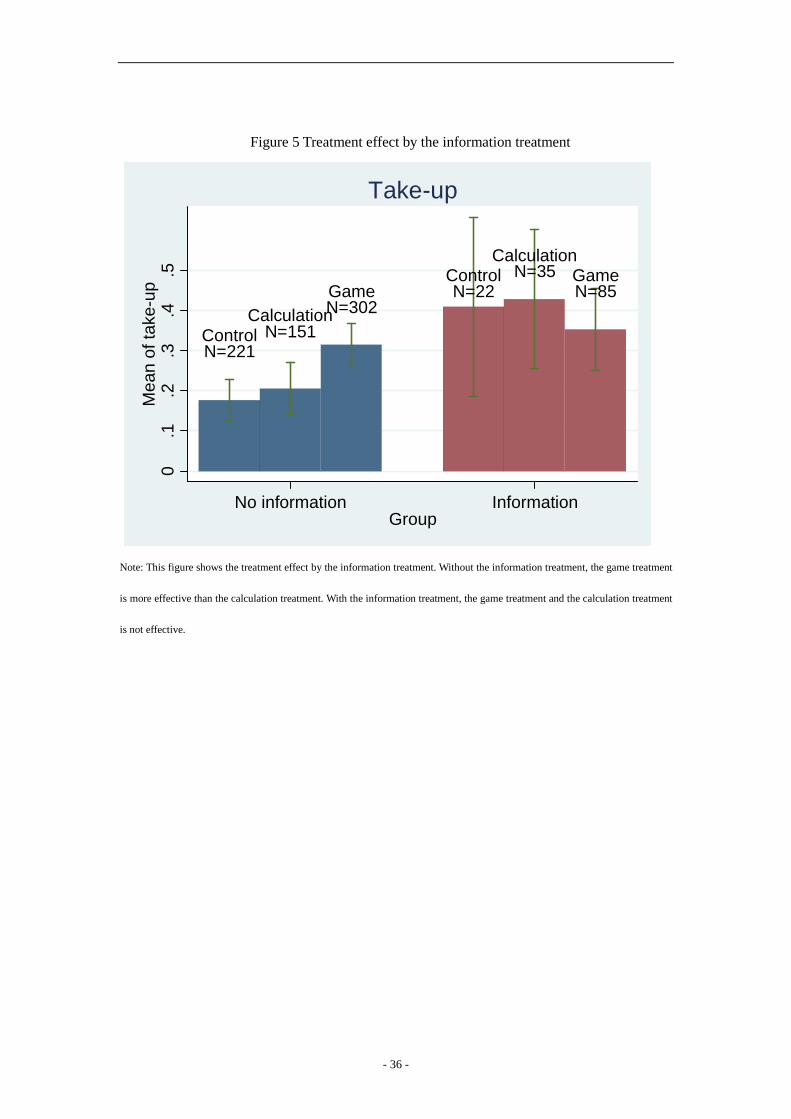
Figure 5 Treatment effect by the information treatment
ControlCalculation
GameControl
CalculationGame
N=221N=151
N=302N=22
N=35N=85
0.1
.2.3
.4.5
Mea
n of
take
-up
No information InformationGroup
Take-up
Note: This figure shows the treatment effect by the information treatment. Without the information treatment, the game treatment
is more effective than the calculation treatment. With the information treatment, the game treatment and the calculation treatment
is not effective.

- 37 -
Figure 6: Take-up by number of hypothetical disasters in the games
Control
Calculation
Game 20% Game 10%
N=243
N=186 N=45
N=65
N=88
N=57
N=45
N=57
N=30
0.1
.2.3
.4.5
Mea
n of
take
-up
Control Calculation 0 1 2 3+ 0 1 2+Number of hypothetical disasters
Take-up by number of hypothetical disasters
Note: the figure shows the insurance take-up conditioning on the number of disasters they experienced during the games. The left
two bars show the take-up of the control group and the calculation group.

- 38 -
Figure 7: Take-up by number of hypothetical disasters in different rounds
Control
Calculation
First 5 rounds
Last 5 rounds
N=243
N=186
N=163N=151
N=61
N=160
N=155
N=60
0.1
.2.3
.4.5
Mea
n of
take
-up
Control Calculation 0 1 2+ 0 1 2+Number of hypothetical disasters
Take-up by number of hypothetical disasters
Note: the left two bars show that the insurance take-up conditioning whether there is a disaster in the first round and last round.
The right two bars show the insurance take-up conditioning on the number of disasters in the first 5 rounds and last 5 rounds.
Appendix

- 39 -
A.1 Simulation of Insurance Take-up under Standard Model
We simulate the take-up decisions with the following steps:
1. Take a uniform draw of α from the interval according to each household’s choices of
riskless options
2. Take two extreme type I error term and difference them to get logistic error term
3. Use the draw of α ,self-reported p and the error term to calculate the insurance decision
of each household and the percentage of take-up in the simulated sample
4. Repeat 1 to 3 for 100 times and calculate the mean and standard deviation of take-up.
A.2 MLE Estimation of Weight Parameters
We estimate 1µ and 2µ with MLE and simulation with the following steps:
1. Take a uniform draw of α from the interval according to each household’s choices of
riskless options
2. Constrain α to be the draw value and p to be the perceived probability of future
disasters from our survey data, then estimate 1µ and 2µ with MLE
3. Redo step 1 and 2 for 100 times to generate 100 1µ and 2µ
4. Compare the distribution of 1µ and 2µ
Option A Option B Choice
1 50 RMB Toss a coin. If it is heads, you get 200RMB. If it is tails, you get nothing.
2 80 RMB Toss a coin. If it is heads, you get 200RMB. If it is tails, you get nothing.
3 100RMB Toss a coin. If it is heads, you get 200RMB. If it is tails, you get nothing.
4 120RMB Toss a coin. If it is heads, you get 200RMB. If it is tails, you get nothing.
5 150RMB Toss a coin. If it is heads, you get 200RMB. If it is tails, you get nothing.
Table A1. Risk Attitude Qustions
Note: Risk attitudes were elicited for all the households with questions in table 1. For those who were assigned to play games,

- 40 -
risk attitudes were elicited after playing insurance games. Households were asked to make five hypothetical decisions to choose
between riskless option A and risky option B. We use the number of riskless options as a measurement of risk averse. The more
the riskless options are chosen, the more the risk averse is.

- 41 -
Specification:Dep. Var.:
Sample:1 2 3 4
Game 20% 0.108 0.119 -0.056 0.107(0.035)*** (0.034)*** -0.159 (0.036)***
Game 10% 0.045 0.120 -0.097 0.036(0.066) (0.086) (0.182) (0.067)
Calculation 0.020 0.012 -0.008 0.020(0.045) (0.048) (0.189) (0.043)
Wald test: β20=β10
p-value 0.2548 0.9956 0.5877 0.2051Obs. 816 674 132 816Omitted TreatmentMean of Dep. Var. forOmitted Treatment:Social-economic Variables Y Y Y YFixed Effects for Village andEnumerator
Y Y Y Y
Log Likelihood -430 -335 -86 -425Pseudo R-square 0.0933 0.1507 0.0329 0.1045
Control
0.198
Table A2. the Effect of Hypothetical Games on Actual Insurance Take-upLogistic Regression
Individual Adoption of Insurance
All Sample
Notes: Dependent variable is individual adoption; standard errors are clustered by 16 natural villages. Robust clustered standard
errors are in the parentheses. *** significant at 1% level; ** significant at 5% level; * significant at 10% level.

- 42 -
Specification:Dep. Var.:
Sample:1 2 3 4 5 6 7 8
Number of HypotheticalDisasters
0.072 0.083 -0.047 0.133
(0.037)* (0.043)* (0.038) (0.067)**
Number of HypotheticalDisasters in First Half ofGame (2011-2015)
-0.026 0.107 0.085
(0.033) (0.058)* (0.038)**
Number of HypotheticalDisasters in Second Half ofGame (2016-2020)
0.075
(0.034)**Interaction Term (dd5) -0.051 -0.075
(0.050) (0.057)Hypothetical Disaster in 2011 -0.134 -0.140
(0.082) (0.105)Hypothetical Disaster in 2012 -0.134 -0.155
(0.048)*** (0.052)***Hypothetical Disaster in 2013 -0.025 -0.030
(0.071) (0.080)Hypothetical Disaster in 2014 0.004 -0.113
(0.056) (0.043)**Hypothetical Disaster in 2015 0.073 0.096
(0.058) (0.057)*Hypothetical Disaster in 2016 0.155 0.164
(0.039)*** (0.044)***Hypothetical Disaster in 2017 -0.053 -0.050
(0.069) (0.082)Hypothetical Disaster in 2018 0.120 0.147
(0.064)* (0.081)*Hypothetical Disaster in 2019 0.016 0.037
(0.079) (0.060)Hypothetical Disaster in 2020 0.141 0.160
(0.063)** (0.064)**
Obs. 375 375 375 375 292 292 292 292Omitted TreatmentMean of Dep. Var. forOmitted Treatment:Social-economic Variables Y Y Y Y Y Y Y YFixed Effects for Village andEnumerator
Y Y Y Y Y Y Y Y
Log Likelihood -214 -213 -213 -206 -160 -158 -158 -150Pseudo R-square 0.0934 0.0966 0.0979 0.1251 0.1219 0.129 0.1307 0.1743
0.198
Control
Table A3. the Effect of Hypothetical Games on Actual Insurance Take-upLogistic Regression
Individual Adoption of Insurance
Game Game with no Information
Notes: Dependent variable is individual adoption; standard errors are clustered by 16 natural villages. Robust clustered standard
errors are in the parentheses. *** significant at 1% level; ** significant at 5% level; * significant at 10% level.

- 43 -
Specification:Dep. Var.:
Sample:1 2 3 4 5 6 7 8 9
Hypothetical Disaster in 2011 -0.134(0.079)*
Number of HypotheticalDisasters in Last Nine Years(2012-2020)
0.032
(0.012)***
Number of HypotheticalDisasters in First Two Years(2011-2012)
-0.102
(0.036)***
Number of HypotheticalDisasters in Last Eight Years(2013-2020)
0.077
(0.026)***
Number of HypotheticalDisasters in First Three Years(2011-2013)
-0.077
(0.034)**
Number of HypotheticalDisasters in Last Seven Years(2014-2020)
0.080
(0.027)***
Number of HypotheticalDisasters in First Four Years(2011-2014)
-0.053
(0.028)*
Number of HypotheticalDisasters in Last Six Years(2015-2020)
0.084
(0.026)***
Number of HypotheticalDisasters in First Five Years(2011-2015)
0.020
(0.033)
Number of HypotheticalDisasters in Last Five Years(2016-2020)
0.067
(0.040)*
Number of HypotheticalDisasters in First Six Years(2011-2016)
0.013
(0.028)
Number of HypotheticalDisasters in Last Four Years(2017-2020)
0.039
(0.044)
Number of HypotheticalDisasters in First Seven Years(2011-2017)
0.005
(0.026)
Number of HypotheticalDisasters in Last Three Years(2018-2020)
0.068
(0.043)
Number of HypotheticalDisasters in First Eight Years(2011-2018)
0.025
(0.027)
Number of HypotheticalDisasters in Last Two Year(2019-2020)
0.057
(0.057)
Number of HypotheticalDisasters in First Nine Years(2011-2019)
0.004
(0.014)
Number of HypotheticalDisasters in Last Year (2020)
0.1108
(0.070)
Obs. 375 375 375 375 375 375 375 375 375Omitted TreatmentMean of Dep. Var. forOmitted Treatment:Social-economic Variables Y Y Y Y Y Y Y Y YFixed effects for village andenumerator
Y Y Y Y Y Y Y Y Y
Log Likelihood -221 -218 -218 -219 -221 -223 -222 -222 -222Pseudo R-square 0.0628 0.0772 0.0763 0.0733 0.0631 0.0563 0.0601 0.0586 0.0586
Control
0.198
Logistic RegressionIndividual Adoption of Insurance
Game
Table A4. the Effect of Hypothetical Games on Actual Insurance Take-up

- 44 -