Instructor:

Dr. Benjamin Thompson

Lecture 9: 10 February 2009

Announcement� Reminder: Homework 3 is due Thursday

Then…� The Wiener Filter

� The LMS Algorithm

Moving On…

� Matlab Demo: Linear Regression

� Matlab Demo: The Wiener Filter

� Matlab Demo: LMS

� Data Sets

Now!� The Iris Classification Problem

� The Sumo-Basketball Player-Jockeys-Footballers Problem

� Stock Market Data

Chapter Four!

� The Multilayer Perceptron

� Developing the MLP

� General MLP Structure

One letter short of being the Irish data set, which is much more interesting.

An Iris By Any Other Name…� This data set is famous for classification

problems

� Three classes of the Iris flower: Setosa, Versicolor, and Virginica

� Rather than just take a picture of an iris to tell what it is, several features were extracted:

� Sepal Length

� Sepal Width

� Petal Length

� Petal Width

� These features alone are enough to classify a given flower as the correct type.

This is not an iris. But it DOES have its petals and sepals labeled!

The Three Irises

Iris Setosa Iris Versicolor Iris Virginica

If I Grabbed This From Wikipedia,

It’s Not Stealing, Right?

Some day we’ll add Professional Underwater Basket Weavers to the list…

The Big Idea� We want to determine what sport an athlete plays

given:

� Weight

� Height

� And Nothing Else!

� The classes:

� Basketball players

� Horse Jockeys

� Sumo Wrestlers

� Soccer Players

This data comes courtesy of David W. Krout, sports enthusiast, Neural Smith, and previous EE456 Instructor

Can You Guess Who Goes Where?

What are some other features that might fully distinguish all the classes?

If any of you create a predictor that actually makes you filthy rich, I hereby claim a 10% “Instructor’s Commission”. It’s in your syllabus, I swear.

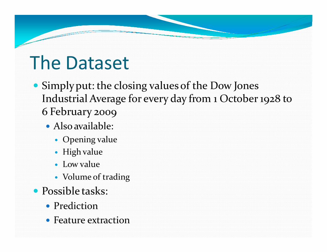
The Dataset� Simply put: the closing values of the Dow Jones

Industrial Average for every day from 1 October 1928 to 6 February 2009

� Also available:

� Opening value

� High value

� Low value

� Volume of trading

� Possible tasks:

� Prediction

� Feature extraction

A Sad Reminder That I Can Never Retire.

Are you guys half as excited as I am?

Ladies and gentlemen, once again, I give you – my good friend and yours – Frank Rosenblatt!

Recall Our Single Neuron Model

Σ

Inputs/Dendrites

Sum-and-

Activation/Neuron

Outputs/Synapses

1x

Nx

2x

3x

⋱

1w

2w

3w

Nw

( )ϕ ⋅ka ky

Remembering Rosenblatt� Recall that the Rosenblatt Perceptron had a few

drawbacks:

� Requires linear separability of the underlying classes

� Threshold activation function only good for discerning between two classes

� Recall: +1 for class 1, -1 (or zero) for class 2

� Simple linear combination of inputs

Oooh, another good band name!

Mental Exercise� Suppose you have more than two classes, but no class

“overlaps” any other class:

1C

2C

3C

4C

•Classes C1 and C2 are

above the blue line

•Classes C3 and C4 are

below the blue line

•Classes C2 and C4 are above the red line

•Classes C1 and C3 are

below the red line

•Any ideas?

Mental Exercise (cont.)� Suppose we run two separate perceptrons:

� Perceptron one is trained to separate classes C1 and C2 from classes C3 and C4� That is, a +1 indicates that the input is in class C1 OR class C2, and a -1

indicates that the input is in class C3 OR C4

3C

4C

Line defined by Rosenblatt weight vector w1

Tx

1C

2C

Mental Exercise (cont.)� Perceptron two is trained to separate classes C2 and C4

from classes C1 and C3� That is, a +1 indicates that the input is in class C2 OR class C4, and a -1

indicates that the input is in class C1 OR C3

1C

3C

4C

Line defined by Rosenblatt weight vector w2

Tx

2C

Mental Exercise (sweaty yet?)� So:

� An input in class C1 will produce a +1 for the first perceptron, AND a -1 for the second perceptron

� An input in class C2 will produce a +1 for the first perceptron, AND a +1 for the second perceptron

� An input in class C3 will produce a -1 for the first perceptron, AND a -1 for the second perceptron

� An input in class C4 will produce a -1 for the first perceptron, AND a +1 for the second perceptron

Mental Exercise (getting winded)� Now in table form!:

Class Perceptron 1 Output

Perceptron 2 Output

C1 +1 -1

C2 +1 +1

C3 -1 -1

C4 -1 +1

Mental Exercise (my brain hurts)

1x

2x

1,1w

1,2w

1,0w

1x

2x

2,1w

2,2w

2,0w

Perceptron 1 Perceptron 2Brand-new Multidimensional Network of Neurons… one might call it a… NEURAL NETWORK!!!

The Math (oh joy!) Behind the

Mental Exercise� If we denote the bias for the 1st perceptron, w1,0, as b1,

and the bias for the 2nd perceptron, w2,0, as b2, then the outputs become:

� y1=sgn(w1,1x1+w1,2x2+w1,0(1)), or

� y1=sgn(w1Tx+b1)

� y2=sgn(w2,1x1+w2,2x2+w2,0(1)), or

� y2=sgn(w2Tx+b2)

� Putting those together yields:

� or [ ]1 1

1 2

2 2

Ty b

y b

= +

sgn w w x ( )T= +y sgn W x b

Bold-faced sgn( ) indicates “vectorized” signum function where the sgn( ) operation is performed on each element of the argument

W is now the weight matrix, rather than the weight vector

By now, your brain should have rock-hard abs.

Because I Just Love Pushing

Things Further Than I Ought…� Suppose two output dimensions doesn’t cut it for us

� Suppose further that we want a single output, just like our good ol’ Rosenblatt Perceptron did for us

� However, now suppose we allow the output to “float” freely (i.e., no threshold unit), such that:

� An output of 1 indicates class C1

� An output of 2 indicates class C2

� An output of 3 indicates class C3

� An output of 4 indicates class C4

Where are we going, and what

am I doing in this handbasket?� Recalling that the outputs of the “neural network” of

perceptrons were limited to +1s and -1s only, we now know that we have ourselves a set of linear equations:

� Since +1, -1 gives us class 1, we can write:

� w1(+1) + w2(-1) + b = 1

� Similarly:

� w1(+1) + w2(+1) +b = 2

� w1(-1) + w2(-1) + b = 3

� w1(-1) + w2(+1) + b = 4

� This is four equations and three unknowns: an overconstrained system

How Convenient…� Solving only the latter three equations yields:

� w1 = -1.0

� w2 = 0.5

� b = 2.5

� Checking our answers:

� (-1)(1) + (0.5)(1) + 2.5 = 2, so an output from class 2 ([-1,1]) will yield an overall output of “2”

� (-1)(-1) + (0.5)(-1) + 2.5 = 3, so an output from class 3 ([-1,-1]) will yield an overall output of “3”

� (-1)(-1) + (0.5)(1) + 2.5 = 4, so an output from class 4 ([-1,1]) will yield an overall output of “4”

� And as it so happens:

� (-1)(1) + (0.5)(-1) + 2.5 = 1, so an output from class 1 ([1,-1]) will yield an overall output of “1”! Yes, I cooked the problem to make this

happen. No, it will not happen in most cases.

Closing With a Picture

1x

2x

1x

2x

So we go from this… …to this!

Circle-with-a-slash indicates a “linear” activation function: the output equals the straight sum of the inputs.

( )1 2

T Ty b= + +w sgn W x b

And we get an output equation that looks like this, if you’ll excuse the sloppy notation!

And by “closing”, I meant “still

going”…� What did we just do?

� We created a perceptron with multiple layers…

� In other words, a multilayer perceptron (MLP)!

� Salient features:

� Input layer

� One or more hidden layers

� Output layer

� bias nodes on each layer after the input layer

� Each element of a given layer is called a node or neuron

� These terms may be (and will be) used interchangeably in this course.

The Hidden Layer� The Hidden Layer is what makes the MLP really tick

� It performs the essential task of feature extraction

� In our example, it extracted the binary “class information” from the continuously-valued input data

� The hidden layer also “warps the manifold of the feature space”, which I swear isn’t a line I stole from Star Trek.

� In other words, rather than a simple hyperplane which splits the feature space in two (allowing us to pick something either “above” or “below” that hyperplane), the hidden layer creates a nonlinear partition of the classes

The Necessity of Nonlinearity� The most fundamental aspect of a true neural network

(in the MLP sense) is the nonlinearity of the hidden layer

� In our example, the sgn( ) functions on each of the hidden nodes

� Let’s examine why this is the case:

� Recall that our output, with nonlinearity intact, is given as

Band name, or boring-but-Oscar-winning weepy drama title?

( )1 2

T Ty b= + +w sgn W x b

The Necessity of Nonlinearity 2:

Perceptron Boogaloo

� Removing the nonlinearity, we would get

� This “simplifies” to

� Dimensional analysis tells us that the first term is just a 2x1 vector, and the second term is just a scalar

� In other words, without the nonlinearity, our MLP devolves into a weight vector plus a bias, which is just a simple, plain-vanilla Rosenblatt Perceptron!

� Suffice it to say, this is not sufficient to perform the classification task we’ve given it!

� The moral of the story: the nonlinearity is a must!

Surprisingly, it didn’t do as well at the box office as its predecessor.

( )1 2

T Ty b= + +w W x b

( ) ( )1 2

T Ty b= + +Ww x w b

…and his second-in-command, Capt. LMS Al Gorithm.

We’ll See This Slide A Lot.

This might be described as a 3x4x5x2 Neural Network. The bias is assumed and thus not counted in the dimensions.

Some Nomenclature: Inputs

and Layers� x is the input vector

� x1 is the first input

� xi is the ith input

� “The nth layer” refers to any type of layer

� “The first layer” always means the input layer

� “The first hidden layer” always means the second layer of a proper MLP

� So “the second layer” is equivalent to “the first hidden layer”

� “The last layer” is the output layer, and is notsynonymous with “the last hidden layer”, which always precedes it by one layer.

Study these next few slides. The development of the learning algorithm for the MLP, while mathematically elegant, is notational hell, and knowing these will make following the next lecture vastly easier

More Nomenclature:

Activations� a1(1) is the activation potential (aka induced local

field, aka neuronal input) of the first neuron of the first hidden layer

� ak(1) is the activation potential of the kth neuron of the first hidden layer

� ak(n) is the activation potential of the kth neuron of the nth hidden layer

� In general, the activation is the weighted sum of all the connected inputs (more on this later)

Haykin uses υinstead of a, but I think a makes more sense contextually speaking.

More Nomenclature: Weights� w1,1(1) is the weight or synaptic connection between

the first input and the first neuron of the first hidden layer.

� wj,k(1) is the weight of the connection between the jth

input and the kth neuron of the first hidden layer

� wj,k(n) is the weight of the connection between the output of the jth neuron on the nth layer and the input of the kth neuron on the (n+1)st layer

� W(n) is the weight matrix between layers n and n+1, whose (j,k)th element is wj,k(n)

Generally, subscript j will always refer to something to the left of something with subscript k

So if something occurs in a temporal order, I’ll try to replicate this in alphabetical order.

More Nomenclature: Bias� b(1) refers to the bias vector feeding into the first

hidden layer

� b1(1) refers to the weight connecting the bias to the first neuron of the first hidden layer

� bk(1) refers to the weight connecting the bias to the kth

neuron of the first hidden layer

� bk(n) refers to the weight connecting the bias to the kth

neuron of the nth hidden layer (or output if n is the last layer)

� b(n) refers to the bias vector feeding the nth hidden layer (or output if n is the last layer)

More Nomenclature: Neuron

Outputs � φφφφ(n) is the output vector of the nth hidden layer

� φ1(1) is the output of the 1st node in the 1st hidden layer

� φk(1) is the output of the kth node in the 1st hidden layer

� φk(n) is the output of the kth node in the nth hidden layer

� We may abuse the notation and use φφφφ(0) to refer to the input vector!

� We use φ to signify the activation function.

� When given, we may use the function itself in place of φ� threshold function θ( )

� sigmoid function σ( )

� signum function sgn( )

Pay close attention to this subtlety!

More Nomenclature� Alternately, rather than φφφφ(n), we may use y(n) and

yk(n) to refer to the same thing

� This makes it clear in the y=f(x) sense that it’s an outputof something

� Finally: o refers to the output vector of the whole neural network

� o1 is the first output node

� ok is the kth output of the neural network

A Look at the First Layer� The input to the first hidden neuron

may be written as:

� The keen observer will note that this is simply an affine operation wTx+b for some w

� From there, it’s easy to see that the activations of the entire first hidden layer can be calculated as:

x

( )1W

( )1b

( ) ( ) ( ) ( )1 1,1 1 ,1 11 1 1 1n na w x w x b= ⋅ + + ⋅ +…

( ) ( ) ( ) ( )

( ) ( ) ( )1

1 1 1 1

1 1 1

T

m

T

= +

= +

a w w x b

a W x b

…

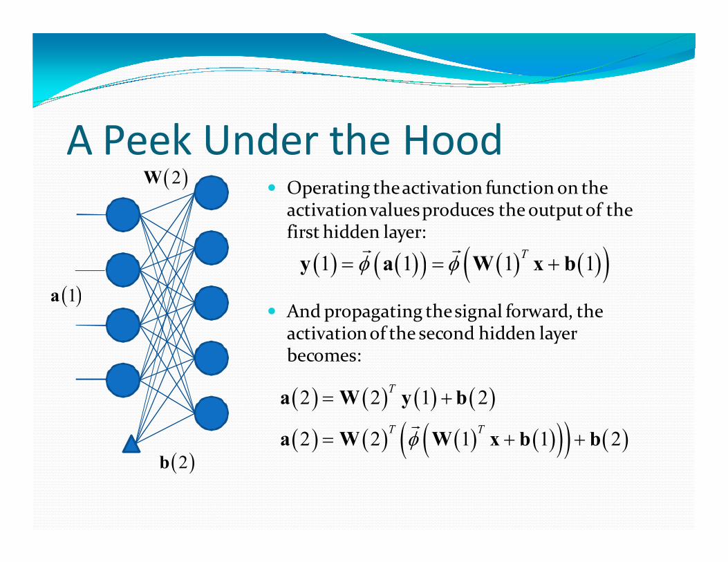
A Peek Under the Hood� Operating the activation function on the

activation values produces the output of the first hidden layer:

� And propagating the signal forward, the activation of the second hidden layer becomes:

( )2W

( ) ( )( ) ( ) ( )( )1 1 1 1Tφ φ= = +y a W x b

� �

( ) ( ) ( ) ( )

( ) ( ) ( ) ( )( )( ) ( )

2 2 1 2

2 2 1 1 2

T

T Tφ

= +

= + +

a W y b

a W W x b b�

( )2b

( )1a

…And the Output Layer� Now we repeat the process for

the next layer:

� Finally, the output layer becomes:

( )2a

( )3W

( )3b

o( ) ( )( )

( ) ( ) ( ) ( )( )( ) ( )( )2 2

2 2 1 1 2T T

φ

φ φ

=

= + +

y a

y W W x b b

�

� �

( ) ( ) ( )

( ) ( ) ( ) ( )( )( ) ( )( ) ( )

3 2 3

3 2 1 1 2 3

T

T T Tφ φ

= +

= + + +

o W y b

o W W W x b b b� �

Note: generally, there is no good reason to add a nonlinearity to the final output neurons, hence the above form.

Forward Propagation

φ

φ

φ

φ

φ

φ

φ

φ

φ

φ

φ

1x

nx

2x

1o

mo

φ

φ

φ

φ

φ

φ

φ

φ

φ

φ

φ

( ) ( ) ( ) ( )( )( ) ( )( ) ( )3 2 1 1 2 3T T Tφ φ= + + +o W W W x b b b� �

( )1W( )3W

( )2W

( )3b( )1b ( )2b

Ding! Your output is ready!