institutions and public sector performance: empirical ... · institutions and public sector...
TRANSCRIPT

Institutions and Public Sector Performance:
Empirical Analyses of Revenue Forecasting
and Spatial Administrative Structures
Inaugural-Dissertation
zur Erlangung des Grades
Doctor oeconomiae publicae (Dr. oec. publ.)
an der Ludwig-Maximilians-Universitat Munchen
2011
vorgelegt von
Bjorn Kauder
Referent: Prof. Dr. Thiess Buttner
Korreferent: Prof. Dr. Gebhard Flaig
Mundliche Prufung: 4. November 2011
Promotionsabschlussberatung: 16. November 2011

Acknowledgements
First of all I would like to thank Thiess Buttner and Gebhard Flaig for their willingness to
supervise my thesis. I am especially indebted to Thiess Buttner for his ongoing support,
encouragement, and inspiration. This fruitful collaboration is reflected particularly in his
co-authorship of Chapters 2 and 3. Moreover, I gratefully acknowledge the Ifo institute
for providing me with an optimal research environment and financial support. I especially
thank my colleagues at the Department of Public Finance and my fellow doctoral students
for contributing to a pleasant working atmosphere. Special thanks go to Nadine Fabritz
for her willingness to help and her kind encouragement. I am also grateful to Christian
Breuer for extensive discussions regarding the political background of all the chapters and
to Alexander Ebertz for his support particularly during the final stage of this dissertation.
Editorial support by Daniel Rees and Deborah Willow is greatly appreciated. I benefited
a lot from comments and suggestions of participants at conferences and workshops in Kiel,
Munich, Nuremberg, and Uppsala, and at seminars at CES and Ifo. I would especially like
to thank Søren Bo Nielsen for insightful discussions and comments on Chapter 4. Last but
certainly not least I would like to thank my parents for their encouragement and support
throughout the entire project.
i

Contents
1 Introduction 1
2 Revenue Forecasting Practices: Differences across Countries and Conse-quences for Forecasting Performance 9
2.1 Introduction . . . . . . . . . . . . . . . . . . . . . . . . . . . . . . . . . . . 10
2.2 Forecasting Performance . . . . . . . . . . . . . . . . . . . . . . . . . . . . 13
2.3 Conditions Faced by Forecasters . . . . . . . . . . . . . . . . . . . . . . . . 19
2.4 Institutions and Independence . . . . . . . . . . . . . . . . . . . . . . . . . 22
2.5 Determinants of Forecasting Performance . . . . . . . . . . . . . . . . . . . 27
2.6 Summary . . . . . . . . . . . . . . . . . . . . . . . . . . . . . . . . . . . . 34
3 Revenue Forecasting in Germany: On Unbiasedness, Efficiency, and Pol-itics 50
3.1 Introduction . . . . . . . . . . . . . . . . . . . . . . . . . . . . . . . . . . . 51
3.2 Investigation Approach . . . . . . . . . . . . . . . . . . . . . . . . . . . . . 53
3.3 Data and Descriptive Statistics . . . . . . . . . . . . . . . . . . . . . . . . 56
ii

3.4 Empirical Results . . . . . . . . . . . . . . . . . . . . . . . . . . . . . . . . 62
3.5 Conclusions . . . . . . . . . . . . . . . . . . . . . . . . . . . . . . . . . . . 71
4 Spatial Administrative Structure and Inner-Metropolitan Tax Competi-tion 80
4.1 Introduction . . . . . . . . . . . . . . . . . . . . . . . . . . . . . . . . . . . 81
4.2 Theoretical Model . . . . . . . . . . . . . . . . . . . . . . . . . . . . . . . . 84
4.3 German Municipalities and Institutions . . . . . . . . . . . . . . . . . . . . 88
4.4 Agglomerations and Empirical Strategy . . . . . . . . . . . . . . . . . . . . 91
4.5 Empirical Results . . . . . . . . . . . . . . . . . . . . . . . . . . . . . . . . 98
4.6 Conclusions . . . . . . . . . . . . . . . . . . . . . . . . . . . . . . . . . . . 106
5 Consolidation of Municipalities and Impact on Population Growth – APropensity Score Matching Approach 117
5.1 Introduction . . . . . . . . . . . . . . . . . . . . . . . . . . . . . . . . . . . 118
5.2 Institutional Background . . . . . . . . . . . . . . . . . . . . . . . . . . . . 121
5.3 Identification Strategy and Data . . . . . . . . . . . . . . . . . . . . . . . . 123
5.4 Empirical Results . . . . . . . . . . . . . . . . . . . . . . . . . . . . . . . . 130
5.5 Conclusions . . . . . . . . . . . . . . . . . . . . . . . . . . . . . . . . . . . 140
6 Concluding Remarks 151
iii

List of Tables
1.1 Cities with the Highest Intensity of Incorporation . . . . . . . . . . . . . . 4
2.1 Descriptive Statistics of Forecast Errors . . . . . . . . . . . . . . . . . . . . 18
2.2 Forecasting Conditions . . . . . . . . . . . . . . . . . . . . . . . . . . . . . 20
2.3 Institutional Characteristics and Independence . . . . . . . . . . . . . . . . 25
2.4 Determinants of Forecast Error . . . . . . . . . . . . . . . . . . . . . . . . 28
2.5 Determinants of Forecasting Precision and Accuracy: Total Revenues . . . 30
2.6 Determinants of Forecasting Precision and Accuracy: Disaggregated Revenues 33
2.7 Timing of Forecasts and Time Span . . . . . . . . . . . . . . . . . . . . . . 43
3.1 Descriptive Statistics . . . . . . . . . . . . . . . . . . . . . . . . . . . . . . 57
3.2 Results on the Forecast Bias: May current / May next / November next Year 63
3.3 Results on Forecast Efficiency I: May current / May next / November nextYear . . . . . . . . . . . . . . . . . . . . . . . . . . . . . . . . . . . . . . . 65
3.4 Results on Forecast Efficiency II: November next Year . . . . . . . . . . . . 66
3.5 Results on Forecast Efficiency III: May current / May next / November nextYear . . . . . . . . . . . . . . . . . . . . . . . . . . . . . . . . . . . . . . . 67
iv

3.6 Results on Politics: May current / May next / November next Year . . . . 70
3.7 Results on the Forecast Bias: November Forecast for the next Year (GDPForecast Error based on Research Institutes) . . . . . . . . . . . . . . . . . 73
3.8 Results on Forecast Efficiency I: November Forecast for the next Year (GDPForecast Error based on Research Institutes) . . . . . . . . . . . . . . . . . 74
3.9 Results on Forecast Efficiency II: November Forecast for the next Year (GDPForecast Error based on Research Institutes) . . . . . . . . . . . . . . . . . 75
3.10 Results on Forecast Efficiency III: November Forecast for the next Year(GDP Forecast Error based on Research Institutes) . . . . . . . . . . . . . 76
3.11 Results on Politics: November Forecast for the next Year (GDP ForecastError based on Research Institutes) . . . . . . . . . . . . . . . . . . . . . . 77
4.1 The Largest German Cities and their Regions (of 50 km) . . . . . . . . . . 95
4.2 Local Business Taxation in Metropolitan Areas of 15 km . . . . . . . . . . 100
4.3 Local Business Taxation in Metropolitan Areas of 25 km . . . . . . . . . . 101
4.4 Local Business Taxation in Metropolitan Areas of 50 km . . . . . . . . . . 103
4.5 Local Business Taxation in Metropolitan Areas with Parameter of 10 % . . 104
4.6 Local Business Taxation in Metropolitan Areas with Parameter of 1 % . . 105
4.7 Descriptive Statistics (Regions of 15 km) . . . . . . . . . . . . . . . . . . . 109
4.8 Descriptive Statistics (Regions of 25 km) . . . . . . . . . . . . . . . . . . . 110
4.9 Descriptive Statistics (Regions of 50 km) . . . . . . . . . . . . . . . . . . . 110
4.10 Descriptive Statistics (Regions 10 %) . . . . . . . . . . . . . . . . . . . . . 111
4.11 Descriptive Statistics (Regions 1 %) . . . . . . . . . . . . . . . . . . . . . . 111
v

4.12 Correlation of the Number of Surrounding Municipalities . . . . . . . . . . 112
4.13 Correlation of the Population per Surrounding Municipality . . . . . . . . 112
4.14 Correlation of the Population Share of the Core City . . . . . . . . . . . . 112
4.15 Correlation of the Population of the Region . . . . . . . . . . . . . . . . . 113
4.16 Local Business Taxation in Metropolitan Areas of 50 km (extended) . . . . 114
5.1 Reforms of the Administrative Structure . . . . . . . . . . . . . . . . . . . 122
5.2 Descriptive Statistics . . . . . . . . . . . . . . . . . . . . . . . . . . . . . . 129
5.3 Treatment Probability . . . . . . . . . . . . . . . . . . . . . . . . . . . . . 132
5.4 Average Treatment Effect on the Treated . . . . . . . . . . . . . . . . . . . 134
5.5 Average Treatment Effect on the Treated (Different Time Periods) . . . . . 135
5.6 Average Treatment Effect on the Treated (Different Sizes) . . . . . . . . . 138
5.7 Balancing Property (Radius Matching) . . . . . . . . . . . . . . . . . . . . 139
5.8 Descriptive Statistics (Incorporation <= 1972) . . . . . . . . . . . . . . . . 142
5.9 Descriptive Statistics (Incorporation > 1972) . . . . . . . . . . . . . . . . . 143
5.10 Descriptive Statistics (Population <= 1500) . . . . . . . . . . . . . . . . . 144
5.11 Descriptive Statistics (Population > 1500) . . . . . . . . . . . . . . . . . . 145
5.12 Balancing Property (One-to-one Matching) . . . . . . . . . . . . . . . . . . 146
5.13 Balancing Property (10-Nearest-Neighbors Matching) . . . . . . . . . . . . 147
5.14 Balancing Property (Kernel Matching) . . . . . . . . . . . . . . . . . . . . 148
vi

List of Figures
1.1 Standard Deviation of Next-Fiscal-Year Forecast Error (in %) . . . . . . . 2
1.2 Relevance of Local Business Tax . . . . . . . . . . . . . . . . . . . . . . . . 3
2.1 Forecast Errors by Country/Institution . . . . . . . . . . . . . . . . . . . . 15
2.2 Forecast Errors by Year . . . . . . . . . . . . . . . . . . . . . . . . . . . . 16
3.1 Relative Forecast Error (in %): Current-Year Forecast May . . . . . . . . . 59
3.2 Relative Forecast Error (in %): Next-Year Forecast May . . . . . . . . . . 59
3.3 Relative Forecast Error (in %): Next-Year Forecast November . . . . . . . 60
4.1 Number of Municipalities per 100 Square Kilometers . . . . . . . . . . . . 90
4.2 The Definition of Agglomerations (First Approach) . . . . . . . . . . . . . 93
4.3 The Definition of Agglomerations (Second Approach) . . . . . . . . . . . . 94
4.4 Local Business Taxation in Germany (“Rate of Assessment”) . . . . . . . . 97
vii

Chapter 1
Introduction
“Don’t make the tax figures seem better than they are”, the president of the German Court
of Auditors remarked in apprehension of budget imbalances – he was concerned about too
optimistic revenue forecasts. The performance of agents in the public sector, such as
revenue forecasters, depends on the design of institutions. Also local politicians react to
incentives originated in institutions: “Certainly, this is local-business-tax cannibalism”
claimed the head of the economics department of the city of Frankfurt. He finds his city
exposed to increased tax competition, induced by tax cuts of surrounding municipalities.
The question arises which institutions cause these statements. Since the institutional
framework determines the decision making of politicians and bureaucrats, the performance
of the public sector hinges crucially on the respective environment.
This book looks at two aspects where the effects of institutions on the performance of
political agents are particularly relevant – one on the country and the other on the local
level. The first concerns the environment in which revenue forecasters work. Since revenue
forecasts are the basis of every budgetary process, they feature prominently in decisions

CHAPTER 1. INTRODUCTION 2
Figure 1.1: Standard Deviation of Next-Fiscal-Year Forecast Error (in %)
US: CBO 10.175
Japan 10.003
US: OMB 9.031
Ireland 7.608
Netherlands 6.203
Germany 5.419
Canada 5.044
Italy 4.626
New Zealand 3.939
Belgium 2.611
France 2.542
Austria 2.279
United Kingdom 1.977
0
2
4
6
8
10
12U
S:
CB
O
Jap
an
US
: O
MB
Irel
and
Net
her
lan
ds
Ger
man
y
Can
ada
Ital
y
New
Zea
lan
d
Bel
giu
m
Fra
nce
Au
stri
a
Un
ited
Kin
gd
om
Figure covers the period from 1995 to 2009 (fewer observations for some countries). CBO – Congres-
sional Budget Office. OMB – Office of Management and Budget.
regarding economic policy. But as Figure 1.1 shows, their quality differs notably across
countries and institutions. This gives rise to the question why this is, and calls for an in-
vestigation into the determinants of forecasting precision. Among these determinants may
be the assignment of the task: While in some countries revenue forecasting is performed
by independent institutions, others produce the figures in their ministries. But also fur-
ther conditions differ that can affect the performance of forecasters and hence the policies
implemented, such as the structure of the tax system or the timing of forecasts. Exploit-
ing variation in these differences allows for identifying institutions that lead to superior
forecasts. Also the information that is provided by the government has to be mentioned
in this context. It enables (superior members of) a government to “optimize” the figures
strategically in order to influence the forecasts in the preferred direction. The question of
whether such manipulation or other biases exist and whether forecasters use all the relevant
information available at the time of the forecast calls for further empirical assessment.

CHAPTER 1. INTRODUCTION 3
Figure 1.2: Relevance of Local Business Tax
Property Tax 4730337 für 2007
Local Business Tax 16039355
Share of Income Tax 8407040
Share of VAT 1698545
15.3%
51.9%
27.2%
5.5%
Property Tax
Local Business Tax
Share of Income Tax
Share of VAT
Diagram shows revenue shares of municipal taxes in the average county-independent city (“Kreis-
freie Stadt”) in 2007. Property Tax comprises Property Taxes A and B. Local Business Tax net of
contributions to higher administrative levels (“Gewerbesteuerumlage”).
But also local politicians react in one way or another to structures they are working in and
upper-level decisions they are “exposed to”. This is particularly relevant in the case of the
local business tax. As is shown in Figure 1.2, this is the most important tax for German
municipalities and – since local politicians decide upon its level – of highest relevance.
Since the tax level influences location decisions of firms and, via the resulting tax revenues,
also the scope for designing local policies, factors that affect the tax-setting behavior of
politicians have to be identified. This leads to the spatial administrative structure of
municipalities in the sense of the shape of their borders. Depending on the position of
a municipality in its region and on the level of fragmentation of such a region, different
tax regimes can result. But borders of municipalities are also subject to reforms. Which
dimension they can have is shown in Table 1.1, which refers to reforms in Germany that
are also utilized in this book. The way politicians react to incorporations of adjacent
municipalities and the hereby induced incentives offered to potentially moving citizens is
a further aspect of interest.

CHAPTER 1. INTRODUCTION 4
Table 1.1: Cities with the Highest Intensity of Incorporation
Pop. 2008 Area 1961 Area 2008 Area Growth
Ansbach 40,454 9.65 99.91 935.34 %Hamm 182,459 24.80 226.24 812.26 %Neustadt an der Weinstraße 53,658 17.68 117.10 562.33 %Wolfsburg 120,538 31.20 204.03 553.94 %Bielefeld 323,615 46.84 257.91 450.62 %Bonn 317,949 31.30 141.22 351.18 %Memmingen 41,050 15.89 70.20 341.79 %Munster 273,875 73.84 302.93 310.25 %Straubing 44,496 19.31 67.58 249.97 %Passau 50,717 19.94 69.55 248.80 %
Only “county-independent” cities are displayed. The mean intensity of incorporation among all
county-independent cities amounts to 112.46 % (area growth), and only a few cities have experi-
enced no incorporations. Area in square kilometers.
Accordingly, this book is concerned with institutions and public sector performance, ap-
plied to the cases of revenue forecasting and the spatial administrative structure of muni-
cipalities. What do these two issues have in common? Regardless of whether one considers
a revenue forecaster or a local politician, both are exposed to circumstances associated
with institutions that are designed and implemented by upper-level politicians. These in-
stitutions entail incentives that crucially influence the behavior of politicians or political
agents. A revenue forecaster may act differently when employed by an independent re-
search institute rather than by a Federal Ministry of Finance. The resulting difference in
the revenue forecast in turn has an impact on the budget process of the government and
hence on the policies implemented (see Chapters 2 and 3). Similarly, a local politician who
decides upon tax policy will behave according to the institutions in which he is employed.
As already mentioned, the politician will presumably set lower taxes when there are more
institutions (here: municipalities) surrounding his home city (Chapter 4). In the case of

CHAPTER 1. INTRODUCTION 5
reforms of spatial administrative structures it is the scope of institutions that is affected,
which particularly influences the expenditure decisions of politicians that in turn have an
impact on the residence decisions of households (Chapter 5). Hence, all chapters emphasize
the link between institutions and the policies resulting from them. Moreover, they are all
concerned with implications for budgets. While revenue forecasting tries to assess future
results of current laws, adjustments of the local business tax rate aim to change the law to
directly affect revenues. Incorporations of surrounding municipalities almost always result
in larger budgets – not least because of more firms being subject to taxation and higher
revenue shares from income and value added taxes.
The book is structured into five more self-contained chapters. The next two chapters ana-
lyze revenue forecasting, Chapters 4 and 5 are dedicated to spatial administrative struc-
tures, and the book ends with some concluding remarks given in Chapter 6.
We start in Chapter 2 by reviewing the practice and performance of revenue forecasting
in selected OECD countries. While the mean forecast error turns out to be small in most
countries, the standard deviation of the forecast error points to substantial differences in
the forecasting performance across countries. In analyzing whether these differences are
associated with differences in the conditions of revenue forecasting, it shows that they are
first of all explained with the uncertainty about the macroeconomic fundamentals. To some
extent they are also driven by country characteristics such as the importance of corporate
and (personal) income taxes. Furthermore, differences in the timing of the forecasts prove
important. To account for differences in the assignment of forecasting, we come up with
an index of the independence from possible government manipulation, which comprises
information on whether private institutes and/or external experts are involved, and on
the provider of the underlying macroeconomic forecast. While controlling for the other
differences, we find that the independence of revenue forecasting from possible government
manipulation exerts a robust, significantly positive effect on the accuracy of revenue fore-

CHAPTER 1. INTRODUCTION 6
casts. Moreover, for the European countries there are signs that forecasting precision has
increased with the establishment of fiscal surveillance by the European institutions. The
results are confirmed when distinguishing between four groups of taxes. It shows that the
forecasting precision is particularly low for income and corporation taxes. For these we
find that the precision strongly depends on the timing of the forecast.
These results motivate to look explicitly into one country. Since independence has proven
to be an important factor in explaining the quality of forecasts, valuable insights can
be gained from considering a number of further variables describing the environment of
forecasting. This is done by analyzing the performance of revenue forecasting in Germany
in the third chapter. Tools provided by the literature on rational forecasting are used to
investigate both unbiasedness and efficiency of the forecasts, but also whether indications
for the relevance of politics can be found. Employing data from 1971 until 2009, we find
forecasts to be unbiased and widely efficient; only with regard to tax law changes there are
signs that available information at the time of the forecast is not utilized in an efficient
way. We find evidence that the effects of tax law changes that are known to the forecaster
are overestimated. When law changes are not yet taken into account by the forecaster,
however, the forecast errors go in the expected direction. While a substantial part of
revenue forecast errors can be explained by GDP forecast errors, there is no evidence that
using the GDP forecast of the German Council of Economic Advisors leads to more efficient
results. The analysis of possible influences of politics on revenue forecasting shows some
room for improvement of the forecasts with respect to the term of office. We find the tax
revenue forecast error to become smaller the longer the government is in office. This might
reflect larger overestimations at the beginning of the rule, in order to convey the impression
that political programs are sufficiently funded.
The second part of this book analyzes the role of institutions on the local level. Chapter 4
considers the impact of the shape of municipalities’ borders on local business tax policy in

CHAPTER 1. INTRODUCTION 7
core cities of agglomerations. First, a model is presented that shows the dependence of the
level of taxation on the spatial administrative structure. Afterwards, data from Germany
are employed to discover the effects of the number and size of municipalities within agglo-
merations. In the definition of agglomerations we rely on the one hand on a distance-based
approach, but further develop a method that is based on cumulative population densities.
The results show that the spatial administrative structure matters for the level of local
business taxation. On the one hand, the core city’s tax rate in a metropolitan area is
lower the more municipalities are situated around the city. The effect is confirmed when
we focus on the average population size of neighboring municipalities rather than on the
sheer number of them, since smaller municipalities imply more competitors. On the other
hand, the tax of the core city is higher the larger its population share in the agglomeration.
Thereby, the result has more power for regions defined wider, since a given share in a large
region is associated with a more powerful position of this city than the same share in
a small region. These empirical results coincide with those results from the theoretical
analysis. Furthermore, they hold irrespective of whether one defines agglomerations based
on distances of surrounding municipalities, or based on cumulative population densities in
the agglomeration.
The fifth chapter looks at adjustments of spatial administrative structures. During the
1960s and 1970s, the number of municipalities in Germany was notably reduced. Many
municipalities located on the outskirts of a city lost their independent status and became
a district of the adjacent core city. This chapter analyzes the consequences of such a
reform on the population development in these city districts. In comparing incorporated
municipalities with those that remained independent, the former are found to perform
better in terms of population growth. This effect is confirmed when differences in states’
population growth rates are taken into account, and becomes stronger for municipalities
that were incorporated later and for smaller municipalities. Among the arguments for the
effects found may be improvements in the infrastructure between city and incorporated

CHAPTER 1. INTRODUCTION 8
municipality or a more efficient provision of public goods in general. Also the location of
past housing programs may play a role. To avoid selection bias by possibly comparing
two groups with different properties, a propensity score matching approach is employed.
This allows us to compare incorporated with still independent communities that had a
similar propensity to be incorporated and, hence, similar characteristics. We find that the
propensity score is basically driven by the distance of the community to the core city, the
size in terms of population and area, and the state to which it belongs. Several methods
of propensity score matching are employed, all of them prove able to reduce the difference
between the group of incorporated and the group of still independent municipalities to a
large and sufficient extent.
Following the four main chapters, this book – as already announced – wraps up with some
concluding remarks provided in Chapter 6.

Chapter 2
Revenue Forecasting Practices:
Differences across Countries and
Consequences for Forecasting
Performance

CHAPTER 2. REVENUE FORECASTING PRACTICES 10
Abstract∗
This chapter reviews the practice and performance of revenue forecasting in selected OECD
countries. It turns out that the cross-country differences in the performance of revenue
forecasting are first of all associated with uncertainty about the macroeconomic fundamen-
tals. To some extent, they are also driven by country characteristics such as the importance
of corporate and (personal) income taxes. Also, differences in the timing of the forecasts
prove important. However, controlling for these differences, we find that the independence
of revenue forecasting from possible government manipulation exerts a robust, significantly
positive effect on the accuracy of revenue forecasts.
2.1 Introduction
When the financial crisis hit the economy of OECD countries in 2008, the fiscal outlook for
most OECD countries deteriorated substantially. On the revenue side, tax receipts turned
out to be much lower than officially predicted. In the US, for instance, the 2008 federal
government revenues turned out to be 7.8 % and 5.5 % below official revenue forecasts
by the Congressional Budget Office from January 2007 and the Office of Management and
Budget from February 2007. For Ireland, the 2008 revenue figure issued by the Department
of Finance in December 2008 turned out to be 13.4 % lower than was predicted a year
earlier. It seems straightforward to relate these forecast errors to the severe recession
that hardly anyone predicted in the first half of 2007 when these forecasts were made.
However, given that these forecasts play an important role in setting up the budget, it
seems interesting to compare forecasting performance across countries and to discuss its
∗This chapter is joint work with Thiess Buettner. It is based on our paper “Revenue ForecastingPractices: Differences across Countries and Consequences for Forecasting Performance,” Fiscal Studies, 31(3), 2010.

CHAPTER 2. REVENUE FORECASTING PRACTICES 11
relationship with different forecasting practices.
Since revenue forecasting is an essential part of budgeting in the public sector, all countries
make efforts to obtain reliable figures for the expected revenues – which is a difficult task.
Preparing revenue forecasts involves not only predictions about macroeconomic develop-
ment but also predictions about the functioning of tax law and its enforcement. Further-
more, there are changes in tax laws and structural changes in the economy that make
forecasting even more difficult. Another possible uncertainty lies in the repercussions of
revenue developments on public spending and the associated macroeconomic consequences.
While these challenges are faced by forecasters in all countries, there are significant dif-
ferences in the practice of revenue forecasting.
In particular, institutional aspects of revenue forecasting differ. In several countries, the
executive branch of the government is directly in charge; other countries delegate the
forecasting task to independent research institutes and emphasize the independence of
forecasting. This raises the question of whether forecasting performance is affected by the
different practices involved. Given the efforts that some countries devote to ensuring inde-
pendence from possible government manipulation, it is particularly interesting to explore
whether this independence has a noticeable impact on the quality of the forecasts.
The performance of revenue forecasting and possible determinants including institutional
aspects have been explored in the literature in different directions.1 Revenue forecasting
has received most attention in the context of US states’ revenue forecasts. Feenberg et
al. (1989), for instance, provide evidence that state revenue forecasts are biased downwards.
More recently, Boylan (2008) finds evidence for biases associated with the electoral cycle.
Bretschneider et al. (1989) focus on the accuracy of revenue forecasts and find that accuracy
is higher in US states with competing forecasts from executive and legislative branches.
1For a recent survey, see Leal et al. (2008).

CHAPTER 2. REVENUE FORECASTING PRACTICES 12
Moreover, Krause, Lewis, and Douglas (2006) provide some evidence that the accuracy
of states’ revenue fund estimates depends systematically on the staffing of the revenue
forecasting teams. As Bretschneider et al. (1989) note, the design of US state governments
has specific features such as balanced–budget rules and a rivalry between executive and
legislative branches of government which may explain some of these results.
International comparisons have mainly centered on forecasts of the budget balance. Re-
cently, the relative performance of deficit forecasts among European countries has been
examined in the context of the European Union’s Stability and Growth Pact. Strauch,
Hallerberg, and von Hagen (2004) consider forecast errors associated with the so-called
“stability programmes” of EU member states, Jonung and Larch (2006) discuss political
biases of the output forecasts and Pina and Vedes (2007) are concerned with institutional
and political determinants of forecast errors for the budget balance. With regard to the
narrower issue of revenue forecasting, international comparisons of practice and perfor-
mance are mainly concerned with developing countries,2 where institutions relevant for
revenue forecasting are underdeveloped.3
Against this background, this chapter provides an analysis of the performance of official
revenue forecasts and its determinants among 12 OECD countries. The selection of coun-
tries aims to capture the seven largest OECD economies (the US, Japan, Germany, Italy,
the UK, France, and Canada). Some further countries were added where detailed infor-
mation about revenue forecasting was available – selected countries in Western Europe
(Austria, Belgium, Ireland, and the Netherlands) and New Zealand.
It turns out that the cross-country differences in the performance of revenue forecasting
are first of all associated with uncertainty about the macroeconomic fundamentals. To
2For example, Kyobe and Danninger (2005).
3See Danninger (2005).

CHAPTER 2. REVENUE FORECASTING PRACTICES 13
some extent, they are also driven by country characteristics such as the importance of
corporate and (personal) income taxes. Also, differences in the timing of the forecasts
prove important. However, controlling for these differences, we find that the accuracy of
revenue forecasting increases with the independence of forecasts from possible government
manipulation.
The following section presents descriptive statistics on the performance of revenue fore-
casting among our sample of OECD countries. Section 2.3 provides an overview of the
different conditions that forecasters face in these countries. Section 2.4 discusses insti-
tutional aspects of the forecasting task among the selected OECD countries and sets up
a simple indicator of the independence of revenue forecasting from possible government
manipulation. Section 2.5 presents empirical evidence on the determinants of forecasting
performance. Section 2.6 provides a short summary.
2.2 Forecasting Performance
A common way to assess the quality of revenue forecasts is to consider the forecast error
defined as the percentage difference between forecasted and realized revenues. A smaller
forecast error is then usually regarded as a better forecast quality. However, it should be
noted that official revenue forecasts are basically used to indicate the revenue constraint
that needs to be taken into account in the preparation of the public budget. Often, the
budget will include expenditures that have a direct or indirect effect on tax revenues. While
foreseeing these effects might result in a smaller forecast error, it is not clear whether this
constitutes an improvement of a forecast that basically aims to provide the policymaker
with information about the revenue constraint before actions are taken. In the discussion
of the revisions of US revenue forecasts, therefore, policy changes are distinguished from

CHAPTER 2. REVENUE FORECASTING PRACTICES 14
(macro)economic and so-called technical sources (Auerbach, 1999) of forecast errors, where
the latter may refer to tax administration or evasion, for instance. However, for most
countries, a decomposition is not available. Therefore the quantitative analysis presented
below is based on the overall forecast error associated with the revenue forecast.
We focus on the official tax-revenue forecasts used for setting up budgets, i.e. we deal with
revenue forecasts for the next fiscal year. In most cases, this implies that we consider a
one-year-ahead forecast error for tax revenues. In some cases, in particular if the fiscal
year differs from the calendar year, the forecast is sometimes issued in the same year as
the fiscal year begins. Since, ultimately, the forecast should indicate the revenue constraint
to the current budget, we define forecast errors as the deviation of the forecasts from the
final revenues reported for the corresponding fiscal year.4 With regard to the time period
covered, note that we include forecasts issued from 1995 until 2009, but for several countries
revenue forecasts were not available for some years and most forecasts were issued in the
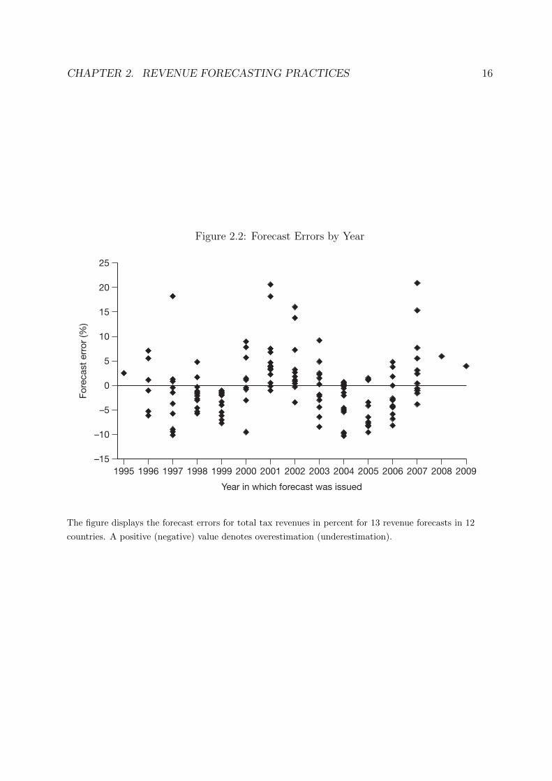
period from 1996 until 2007.5 The forecast errors are depicted in Figures 2.1 and 2.2, where
each point represents a single forecast error. Note that in Figure 2.1 the forecast errors are
arranged in descending order of the respective standard deviation and that in Figure 2.2
they are arranged according to the year in which the forecasts were issued.
At first sight, Figure 2.1 seems to suggest that in most cases there is some underestimation
going on. But there are also instances of large overestimations. For instance, the US
Congressional Budget Office (CBO) issued a revenue forecast in January 2001 for the
2001-02 fiscal year, which started on October 1, 2001, amounting to USD 2,236 billion.
Two years later, revenues turned out to be only USD 1,853 billion. Hence the forecast was
about 20.6 % higher than realized revenues. A revenue forecast by the Japanese Ministry of
4Only for the most recent Canadian forecast, final revenues were not available.
5See Table 2.7 in the appendix for an overview of the actual forecasts used. In the case of the Nether-lands, due to structural breaks, just five years are considered.

CHAPTER 2. REVENUE FORECASTING PRACTICES 15
Figure 2.1: Forecast Errors by Country/Institution
B & K, Figure 1
B & K, Figure 2
CBO – Congressional Budget Office. OMB – Office of Management and Budget.
The figure displays the forecast errors for total tax revenues in percent for up to 13 years in each
country, each point representing one forecast. Forecast errors for 2008 are highlighted with a rhombus.
A positive (negative) value denotes overestimation (underestimation). The forecasts are arranged in
descending order of the standard deviation of the respective forecast errors. The two US forecasts
only refer to federal taxes.
CHAPTER 2. REVENUE FORECASTING PRACTICES 16
Figure 2.2: Forecast Errors by Year
B & K, Figure 1
B & K, Figure 2
The figure displays the forecast errors for total tax revenues in percent for 13 revenue forecasts in 12
countries. A positive (negative) value denotes overestimation (underestimation).

CHAPTER 2. REVENUE FORECASTING PRACTICES 17
Finance from December 2007 for the fiscal year 2008-09 turned out to overestimate actual
revenues by as much as 21.0 %. While several other forecasts associated with 2008 (marked
with a rhombus) also turned out to be overoptimistic, errors of this magnitude are rare.
According to Figure 2.2, the forecast errors show a marked cyclical pattern.
Table 2.1 provides figures for the mean forecast error. A positive sign indicates an over-
estimation of revenues, a negative sign an underestimation. In all cases except Germany,
Japan, and the CBO forecast in the US, there is a slight underestimation of revenues. The
largest difference from zero is found for the Netherlands, which shows an underestimation
of 3.4 % on average. However, given the large standard deviations, statistically the means
are not significantly different from zero.
The large differences in the standard deviation of the forecast errors (SDFE) point to
substantial differences in the precision of forecasts. As can be seen in Column (3) of Table
2.1 the highest precision is achieved in the UK and Austria, while we find the lowest
precision in the US and Japan.
Table 2.1 also reports the root mean squared forecast error (RMSFE), which is a common
summary measure of forecasting accuracy, based on a quadratic loss function regarding
forecast errors.6 Note that the RMSFE is equivalent to a combination of the standard
deviation of the forecast error and the mean forecast error.7 However, as documented by
Table 2.1, the standard deviation of the forecast error and the RMSFE of revenue forecasts
do not show large differences.
6See, for example, Clements and Hendry (2002) and Wallis (2008).
7The mean squared forecast error (MSFE) can be decomposed into the square of the mean of theforecast error (MNFE) and the square of the standard deviation of the forecast error (SDFE) (for example,Clements and Hendry (1998)). Formally, ignoring adjustments for the degrees of freedom, we have
MSFE ' MNFE2
+ SDFE2.
Taking the square root yields the root mean squared forecast error: RMSFE ≡√MSFE .

CHAPTER 2. REVENUE FORECASTING PRACTICES 18
Table 2.1: Descriptive Statistics of Forecast Errors
Country MNFEa MNAFEb SDFEc RMSFEd Obs. (Fiscal-) Years(1) (2) (3) (4) (5) (6)
Austria -0.037 1.880 2.279 2.162 10 1997-2006Belgium -0.432 2.179 2.611 2.545 13 1996-2008Canada -2.711 4.278 5.044 5.553 13 1997/98-2009/10France -1.151 2.290 2.542 2.672 10 1999-2008Germany 1.308 4.458 5.419 5.351 12 1997-2008Ireland -0.536 6.271 7.608 7.274 11 1998-2008Italy -2.297 3.716 4.626 4.973 11 1998-2008Japan 2.578 8.076 10.003 9.918 12 1997/98-2008/09Netherlands -3.403 5.265 6.203 6.509 5 2000-2002, 2005-2006New Zealand -1.535 3.465 3.939 4.058 11 1997/98-2007/08United Kingdom -0.213 1.516 1.977 1.897 11 1997/98-2007/08USA: CBO 0.807 8.361 10.175 9.775 12 1996/97-2007/08USA: OMB -0.472 7.347 9.031 8.659 12 1996/97-2007/08
Average -0.623 4.546 5.497 5.488 11
CBO – Congressional Budget Office. OMB – Office of Management and Budget.aMean of the one-year-ahead forecast error for total revenues in percent. A positive (negative)
value denotes overestimation (underestimation).bMean absolute forecast error.cStandard deviation of the forecast error.dRoot mean squared forecast error.

CHAPTER 2. REVENUE FORECASTING PRACTICES 19
2.3 Conditions Faced by Forecasters
An assessment of the considerable differences in the accuracy of forecasts needs to take
account of the different conditions faced by the forecasters. First of all, this is an issue of the
point in time when the forecast is made. Across countries, there are important differences
in the time span between the official forecast and the beginning of the forecasted period,
i.e. the beginning of the forecasted fiscal year (see Column (1) of Table 2.2). Actually, the
median varies between less than 1 month and 9.5 months.
An important source of differences lies in countries’ tax structures. In particular, the
degree of differentiation of the tax system might matter. Rather than relying on a few
large taxes, a country might employ a variety of smaller tax instruments. Provided that
the different tax instruments relate to tax bases that are not closely correlated, this might
reduce the revenue risks associated with the tax system. Therefore, forecasting the revenues
of a large variety of small taxes might be easier than predicting the revenues in a system
that relies on a small number of large taxes. To capture the differentiation of the tax
structure, we use an indicator of the number of taxes based on OECD Revenue Statistics.
More specifically, we employ the most detailed classification of taxes and, starting with the
smallest taxes, count the number of taxes needed to account for 50 % of all tax revenues.8
Of course, this measure is only informative if the individual taxes are really different in
the above sense. Moreover, comparing the number of taxes across countries raises difficult
problems of classifying taxes and the OECD classification matches the various tax systems
to different extents. Nevertheless, relying on this classification, Column (2) of Table 2.2
indicates that there are large differences across countries.
Some types of taxes might be more difficult to predict than others. For instance, we might
8While this measure is concerned with 50 % of all tax revenues, note that the results are found to berobust against choosing other fractions of tax revenues.

CHAPTER 2. REVENUE FORECASTING PRACTICES 20
Table 2.2: Forecasting Conditions
Country Time Span Taxes for GDP Forecast error(Median)a 50 % rev.b MNFEc SDFEd RMSFEe
(1) (2) (3) (4) (5)
Austria 3.5 71.1 -0.209 1.134 1.096Belgium 2.5 53.4 0.072 1.249 1.202Canada 1.5 34.3 0.114 1.837 1.768France 3.5 103.3 0.185 0.910 0.883Germany 7.5 38.3 0.284 0.987 0.987Ireland 0.5 20.3 -0.387 2.628 2.536Italy 5.5 48.1 0.518 1.122 1.189Japan 3.5 36.0 0.393 1.688 1.664Netherlands 9.5 41.1 0.252 1.605 1.458New Zealand 1.5 19.6 -0.334 1.757 1.708United Kingdom 0.5 41.4 -0.544 0.915 1.028US: CBO 8.5
22.0 -0.280 1.365 1.336US: OMB 8
Averagef 4.1 44.1 0.000 1.433 1.409
CBO – Congressional Budget Office. OMB – Office of Management and Budget.aMedian time period between the forecast and the beginning of the forecasted period in months,
taken from the various national sources listed in the appendix.bNumber of taxes needed to account for 50 % of revenues in the respective country, based on OECD
Revenue Statistics.cMean of the one-year-ahead forecast error for gross domestic product in percent. A positive (neg-
ative) value denotes overestimation (underestimation).dStandard deviation of the forecast error.eRoot mean squared forecast error.fMedian time span and statistics for the GDP forecast error are weighted by number of observa-
tions.

CHAPTER 2. REVENUE FORECASTING PRACTICES 21
expect that there are significant differences in the forecast accuracy between forecasting
corporation or personal income taxes and forecasting sales and value added taxes. This
calls for a separate analysis of forecast errors according to the type of tax. The empirical
analysis below therefore distinguishes four groups of taxes: personal income, corporation,
value added and sales, and other taxes. This decomposition is also useful since the revenue
forecasts are usually prepared for aggregates of individual taxes, especially if these taxes
share the same source or taxpayer. This partly reflects the need to employ up-to-date
information on current revenues, which is available usually on a source basis.
Another potentially important reason for differences in the forecast errors is related to un-
certainty about the business cycle and macroeconomic development. This uncertainty is of
particular importance not only because almost all taxes are affected by the macroeconomic
environment. A typical feature of revenue forecasting is that taxes that are strongly driven
by macroeconomic developments, such as corporation taxes or wage and income taxes,
are forecasted using indirect methods. Predominantly, the elasticity method is employed,
where some previously estimated elasticity is used to predict revenue growth based on the
predicted development of GDP or its components.9
Columns (3) to (5) of Table 2.2 provide some statistics for macroeconomic uncertainty for
each of the different countries. Note that, as with the revenue forecasts, we are relying
on the relative forecast error in percentage points. For instance, the mean forecast error
of -0.544 for the UK indicates that, on average, predicted GDP was about half a percent-
age point lower than actual GDP.10 Note that the GDP forecasts are not taken from the
same source as the above official revenue forecasts. This is important since in some cases
the macroeconomic predictions used by the forecasters are based on their own assessment,
while in other cases the macroeconomic forecasts of the government are used (see Sec-
9For an overview of methods of revenue forecasting, see King (1993).
10As in the case of revenue forecasts, the forecast error is computed relative to final figures.

CHAPTER 2. REVENUE FORECASTING PRACTICES 22
tion 2.4). Conditioning on these predictions would not allow us to capture the impact of
possible government manipulation. Therefore, we resort to the German Council of Eco-
nomic Advisors, an independent body which annually issues forecasts of macroeconomic
developments including GDP for a large group of countries.11
Uncertainty about revenues also stems from changes in tax law. The immediate “mechani-
cal” effects of tax law changes are often difficult to estimate. In addition, changes in tax law
exert all sorts of behavioral effects with revenue consequences that are hard to quantify.12
This implies that revenue forecasts tend to be much more difficult in the presence of tax
law changes. While this may suggest attempting to capture revenue effects of major tax
reforms, we have not been able to collect data on revenue estimates for tax reforms. But
we should note that there is also uncertainty about which tax law changes will actually be
implemented. In some countries, it is common practice not only to include in the revenue
forecasts those tax law changes that are already enacted but also to include changes that
are agreed within the government (Austria, the Netherlands) or noted in the budget plan
(Ireland). If these changes are postponed, amended, or withdrawn, large forecast errors
may occur even if the revenue estimate of the reform that was initially intended was correct.
2.4 Institutions and Independence
A basic institutional aspect of revenue forecasting is the assignment of the forecasting task
to specific institutions. Interestingly, forecasting is not always assigned to a department
of the government or, more precisely, to the executive branch of the government. Only in
11An advantage of these forecasts is that the one-year-ahead forecasts are issued every year in November,so there are no timing differences across countries and time.
12For a discussion of “dynamic scoring” in revenue estimation, see Adam and Bozio (2009) and Auerbach(2005).

CHAPTER 2. REVENUE FORECASTING PRACTICES 23
about half of the 13 forecasts surveyed in this chapter is it the Ministry of Finance (Belgium,
France, Ireland, Italy, Japan) or the Treasury (New Zealand, the UK) that is responsible.13
In most other cases, forecasting is assigned to a group representing different institutions,
not only the executive branch. Some countries even assign the primary responsibility
for revenue forecasting to independent research institutes (the Netherlands) and limit the
influence of the executive branch such that it merely consults forecasters. In the other
countries, even if the Ministry of Finance or another part of the executive is responsible,
external experts from academia or forecasting agencies are often included in the forecasting
group.
The efforts to involve institutions that are not part of the government or external experts
are usually justified as a means to raise the independence of revenue forecasting from
possible manipulation by and strategic influence of the government. Several countries
explicitly produce consensus forecasts, where all institutions and experts involved have
to agree on the forecast (for example, Austria and Germany). However, the extent to
which forecasting is independent from government manipulation depends not only on the
assignment of forecasting responsibility but also on whether revenue forecasting is based
on government predictions for macroeconomic development, as is the case with the official
German forecast.
Table 2.3 presents information about how revenue forecasting differs with respect to these
issues. The first column indicates whether the government (= 0), research institutes (= 1)
or both jointly (= 0.5) are responsible for the forecast. In some cases, no research institutes
are involved but, in order to preserve a certain degree of independence, external experts
are consulted (see Column (2)). This is the case for the US forecasts of the Congressional
Budget Office (CBO) and the Office of Management and Budget (OMB). In the case of the
UK, a value of 0.5 is entered, in order to take account of the reported partial consultation of
13For a detailed list of sources for the various forecasts covered, see the appendix.

CHAPTER 2. REVENUE FORECASTING PRACTICES 24
experts.14 A figure of 0.5 is also entered for Germany, in order to account for the additional
participation of the German central bank. For the Netherlands, a figure of -1 is entered to
take account of the consulting participation of the Ministry of Finance, which may tend to
reduce independence. The third column of the table provides information about the source
of the macroeconomic forecast. A value of 1 indicates that an external forecast is used.
By summing across the first three columns of Table 2.3, we obtain a simple indicator of
the independence of revenue forecasting. The first column is weighted by 1; the second
and third columns are weighted by 0.25. The rationale behind this weighting is the follow-
ing: a revenue forecast that is conducted by a research institute without any government
experts involved would display the maximum level of independence (= 1). A government
forecast that includes external experts and employs an external macroeconomic forecast
would obtain a medium level of independence (= 0.5). A government forecast without any
external experts and without an external macroeconomic forecast would be assigned the
lowest level of independence (= 0).
While the indicator varies from zero (= no independence) to unity (= full independence),
in our sample of countries the highest degree of independence is 0.75. As can be seen,
the indicator is highest for the Netherlands and Austria, followed by Germany. A small,
but positive, level of independence can be found in Canada, New Zealand, Belgium and
the UK. The US case is somewhat special since here two separate forecasts exist. One
is conducted by the OMB, which assists the executive branch; the other is conducted by
the CBO, which is assigned to the legislative branch. While their incentives to manipulate
forecasts strategically might differ, our indicator of independence, which is simply assessing
the institutional conditions, assigns a low value of independence to both of them.15
14Interestingly, the UK government has recently established the Office for Budget Responsibility to“make an independent assessment of the public finances and the economy for each Budget and Pre-BudgetReport” (see www.hm-treasury.gov.uk/data obr index.htm).
15Bretschneider et al. (1989) argue that the existence of two separate forecasts by the legislative and

CHAPTER 2. REVENUE FORECASTING PRACTICES 25
Table 2.3: Institutional Characteristics and Independence
Research Ext./Gov. Macroecon. Indepen-Country institutesa expertsb forecastc denced
Austria 0.5 0 1 0.75Netherlands 1 -1 0 0.75Germany 0.5 0.5 0 0.625Belgium 0 0 1 0.25Canada 0 0 1 0.25New Zealand 0 1 0 0.25US: CBO 0 1 0 0.25US: OMB 0 1 0 0.25United Kingdom 0 0.5 0 0.125France 0 0 0 0.00Ireland 0 0 0 0.00Italy 0 0 0 0.00Japan 0 0 0 0.00
aThis column indicates whether the government (= 0), research institutes (= 1) or both jointly (=
0.5) are responsible for the forecast.bThis column indicates whether external experts (= 1) or government experts (= -1) are involved.
For the UK, a value of 0.5 is entered in order to take account of the reported partial consultation
of experts. In Germany, a figure of 0.5 is entered in order to account for the participation of the
central bank.cThis column provides information about whether an external macroeconomic forecast is used.
(The appendix contains a list of various national sources providing this information.)dThe degree of independence is obtained as a weighted sum of the first three columns. The first
column is weighted by 1 and the second and third columns are weighted by 0.25 (see text).

CHAPTER 2. REVENUE FORECASTING PRACTICES 26
The general composition of the index, with its emphasis on research institutes, external
experts, and the source of the macroeconomic forecast, reflects key institutional charac-
teristics of revenue forecasting. Yet the weights used to aggregate the information about
these institutional aspects are somewhat arbitrary. Therefore we conducted some robust-
ness checks where the weights for external experts and external macroeconomic forecasts
were increased or decreased. With regard to the ranking, however, only minor changes
were found. We will come back to this issue in Section 2.5, where we explore whether the
index of independence has sufficient informational content to help explain the observed
forecasting performance.
Though we include several European countries, the index does not take account of the fiscal
surveillance by EU institutions. Since 1999, due to the Stability and Growth Pact (SGP),
EU member states are required to submit budgetary projections including revenue forecasts
every year to the European Commission and the Ecofin Council. The forecasts also play
a role in the Excessive Deficit Procedure, which defines sanctions for member states that
continuously violate the agreed fiscal rules. It should be noted, however, that the purpose of
the corresponding revenue forecasts is different: they are not issued to set up and justify the
budget plan. Rather, these projections provide the European Commission and the Ecofin
Council with necessary information for the purpose of surveillance of budgetary positions
and economic policies. Nevertheless, the existence of a supranational body discussing and
standardizing the member states’ revenue forecasts might well have implications for the
national governments’ revenue forecasts. By including indicators for EU countries in the
time period starting in 1999, the empirical analysis in Section 2.5 tests for a possible impact
on the performance of revenue forecasts.
executive branches exerts a positive effect on forecasting accuracy, in particular when both forecasts areforced into a consensus. This is, however, not the case with the OMB and the CBO.

CHAPTER 2. REVENUE FORECASTING PRACTICES 27
2.5 Determinants of Forecasting Performance
Having outlined differences in forecasting conditions and practices, let us finally turn to
the question of to what extent these are associated with the large differences in forecasting
performance noted in Section 2.2. In a first step, we consider the level of the revenue
forecast error and test for the presence of forecast biases. Table 2.4 provides the results.
Column (1) indicates that the overall mean or average forecast error is not significantly
different from zero. The specification in Column (2) takes account of the panel structure of
the data and allows for institution-specific differences in a potential bias – which prove not
significant, however. To take account of the difficulties in predicting the macroeconomic
environment, Columns (3) and (4) condition on the one-year-ahead GDP forecast error for
each country. It shows a strongly significant impact indicating that an unpredicted increase
in GDP by 1 % results in an increase of revenues by almost 2 %. According to Column (3),
the average conditional forecast is not significantly different from zero. When we allow the
average forecast error to differ between forecasting institutions (Column (4)), we find that
only the forecasts for Canada and Italy show significant biases. In both cases, conditional
on the forecast error associated with the GDP forecast, the estimation indicates that, on
average, forecasts have been too pessimistic.
In order to explore whether differences in the forecast errors can be assigned to the forecast-
ing institutions, in Columns (5) and (6) we replace the dummies with a set of institution-
specific indicators, most of which are timeinvariant. The set of indicators includes the time
span between the forecast and the forecasted period, the indicator of the differentiation of
the tax structure and the indicator of the independence of forecasting institutions. How-
ever, none of these indicators is significant. While not shown, note that we also tested for
some specific effect for European countries, which are required from 1999 onwards to report
revenue forecasts to European institutions. Even if we allow the coefficients for the Eu-

CHAPTER 2. REVENUE FORECASTING PRACTICES 28
Table 2.4: Determinants of Forecast Error
(1) (2) (3) (4) (5) (6)
Constant -.486 -.441 .171 2.65(.517) (.463) (4.02) (3.62)
GDP forecast error 1.89 ??? 1.99 ??? 1.92 ???
(.316) (.323) (.322)Time span .091 .000
(.167) (.150)log(No. of taxes -.166 -.879for 50 % of revenue) (1.12) (1.01)Independence -.308 .326
(2.29) (2.06)Austria -.037 .380
(1.98) (1.75)Belgium -.432 -.576
(1.73) (1.53)Canada -2.71 -2.94 ?
(1.73) (1.53)France -1.15 -1.52
(1.98) (1.75)Germany 1.31 .743
(1.81) (1.60)Ireland -.536 .234
(1.88) (1.67)Italy -2.30 -3.33 ??
(1.88) (1.67)Japan 2.58 1.80
(1.80) (1.60)Netherlands -3.40 -3.90
(2.80) (2.47)New Zealand -1.54 -.871
(1.88) (1.67)United Kingdom -.213 .869
(1.88) (1.67)US: CBO .807 1.36
(1.80) (1.60)US: OMB -.472 0.84
(1.80) (1.60)
R2 0.000 0.067 0.202 0.279 0.003 0.207Observations 143 143 143 143 143 143
Dependent variable: One-year-ahead forecast error for total tax revenues. Standard errors in
parentheses. A single star denotes significance at the 10 % level, two stars at the 5 % level, and
three stars at the 1 % level.

CHAPTER 2. REVENUE FORECASTING PRACTICES 29
ropean countries to differ in the time period from 1999 onwards, no significant differences
are found.
The failure to find significant effects of institutional characteristics and country characte-
ristics on the mean forecast error does not necessarily indicate that they do not exert any
effect on revenue forecasts. Certainly, in the process of setting up the budget, a government
or parliament is tempted to manipulate the revenue forecast and to underestimate or
overestimate revenues. Yet a sustained manipulation in one direction, which would show
up in a significant bias of the forecasts, hardly affects rational agents’ beliefs and merely
undermines the credibility of the official forecast.16
In a second step of the analysis, we explore the differences in forecasting performance using
measures of forecast precision and accuracy. More precisely, we consider the standard
deviation of the forecast error, which is an indicator of the precision of forecasts, and
the root mean squared forecast error, which is a common summary statistic of forecast
accuracy. The first two specifications in Table 2.5 explore whether differences in forecasting
conditions show some significant effects on the precision of the forecasts, measured by
the SDFE for total tax revenues. Column (1) just includes indicators of macroeconomic
uncertainty and of the time span between the forecast and the beginning of the forecasted
period. The results confirm a strong impact of macroeconomic uncertainty measured by the
standard deviation of the GDP forecast error. They also indicate that precision decreases
considerably with the time span: every additional month increases the standard deviation
by three-quarters of a percentage point. In Column (2), we include our indicator for
the differentiation of the tax system into single taxes. The negative sign indicates that
forecasting is more precise in countries where the number of taxes is larger. However, the
16Consistent with this view, the literature developing models of rational forecast bias relies on settingsnot with one but with multiple forecasting agents, where individual forecasters have incentives to dif-ferentiate their forecasts from those of other forecasters (see, for example, Laster, Bennett, and Geoum(1999)).

CHAPTER 2. REVENUE FORECASTING PRACTICES 30T
able
2.5:
Det
erm
inan
tsof
For
ecas
ting
Pre
cisi
onan
dA
ccura
cy:
Tot
alR
even
ues
Dep
enden
tva
riab
leSD
FE
RM
SF
E(1
)(2
)(3
)(4
)(5
)(6
)(7
)(8
)(9
)(1
0)
Con
stan
t-.
669
7.04
.892
7.16
.665
.905
2.74
3.66
2.22
-.37
2(1
.78)
(7.4
7)(1
.67)
(6.3
8)(1
.56)
(1.8
1)(1
.68)
(6.2
2)(1
.53)
(5.7
2)T
ime
span
.734
???
.635
???
.861
???
.773
???
.887
???
.830
???
.772
???
.762
???
.755
???
.785
???
(.19
0)(.
210)
(.17
1)(.
192)
(.16
7)(.
177)
(.15
2)(.
175)
(.13
0)(.
151)
log(
No.
ofta
xes
-1.6
3-1
.34
-.21
6.5
84fo
r50
%of
reve
nue)
(1.5
4)(1
.32)
(1.3
9)(1
.24)
Indep
enden
cea
-4.4
0?
-4.1
9?
-4.8
8??
-3.6
1?
-3.8
9?
-3.8
8?
-3.4
4??
-3.4
2?
(2.0
0)(2
.01)
(2.0
0)(1
.94)
(1.7
2)(1
.84)
(1.4
7)(1
.55)
EU
-SG
P-2
.15?
-2.0
5-2
.13??
-2.3
9?
(1.0
3)(1
.27)
(.87
3)(1
.07)
SD
FE
for
GD
P4.
36??
3.08
4.03
??
3.00
?4.
08??
4.02
??
3.34
??
3.21
??
(1.2
0)(1
.69)
(1.0
3)(1
.44)
(.98
4)(1
.09)
(.93
7)(1
.32)
RM
SF
Efo
rG
DP
3.66
???
4.10
??
(.87
8)(1
.30)
R2
0.67
70.
713
0.79
00.
814
0.80
50.
767
0.86
40.
864
0.89
40.
897
adj.
R2
0.61
20.
617
0.72
00.
721
0.74
10.
689
0.79
60.
767
0.84
10.
824
Obse
rvat
ions
1313
1313
1313
1313
1313
Dep
end
ent
vari
able
inC
olu
mn
s(1
)-(8
)is
the
stan
dard
dev
iati
on
of
on
e-ye
ar-
ah
ead
fore
cast
erro
rfo
rto
tal
tax
reve
nu
es.
Colu
mn
s(9
)an
d(1
0)
focu
son
the
root
mea
nsq
uar
edfo
reca
ster
ror.
Wei
ghte
dle
ast
squ
are
ses
tim
ate
sta
kin
gacc
ou
nt
of
the
nu
mb
erof
fore
cast
sco
nsi
der
edin
the
com
pu
tati
onof
the
stan
dar
dd
evia
tion
.R
obu
stst
an
dard
erro
rsin
pare
nth
eses
.A
sin
gle
star
den
ote
ssi
gn
ifica
nce
at
the
10
%le
vel
,tw
ost
ars
atth
e5
%le
vel,
and
thre
est
ars
atth
e1
%le
vel.
a)
Colu
mn
(5)
pro
vid
esre
sult
sfr
om
asp
ecifi
cati
on
wh
ere
the
index
of
ind
epen
den
ceu
ses
ah
igh
erw
eigh
tfo
rex
tern
alm
acro
econ
omic
fore
cast
san
dex
tern
al
exp
erts
.C
olu
mn
(6)
refe
rsto
asp
ecifi
cati
on
wh
ere
the
ind
exu
ses
alo
wer
wei
ght
for
exte
rnal
mac
roec
onom
icfo
reca
sts
and
exte
rnal
exp
erts
.

CHAPTER 2. REVENUE FORECASTING PRACTICES 31
effect is not significant.
Columns (3) and (4) show the same specifications augmented with the indicator of the
independence of revenue forecasting. While the results from Columns (1) and (2) are
confirmed, we find that the precision of the forecast is positively associated with the inde-
pendence from possible government manipulation. The coefficient of determination (R2)
for the specification in Column (3) indicates that about 80 % of the variation in the pre-
cision of the forecasts can be associated with the time span, macroeconomic uncertainty
and the degree of independence.
Since the indicator of independence rests on a weighted sum of three institutional charac-
teristics, we conducted some robustness tests using different weights. However, the results
do not indicate major differences. If the weights for external experts and external macro-
economic forecasts are increased or decreased by 0.1, for instance, all effects are confirmed
(see Columns (5) and (6)).
To capture separate fiscal forecasting requirements according to the Stability and Growth
Pact, Columns (7) and (8) include an indicator for EU countries (EU-SGP). It captures
the share of forecasts for European countries that were issued in the time period from 1999
onwards, when regular reports have to be filed for European institutions. Interestingly,
EU-SGP shows a significantly negative effect, suggesting that the precision of revenue
forecasting has generally increased in the presence of budgetary surveillance by the Eu-
ropean Union. Yet a causal interpretation seems problematic, since the formation of the
European monetary union might have exerted separate effects on the forecasting task.
Columns (9) and (10) report results of specifications where we replace the standard de-
viation of the forecast error with the root mean squared forecast error. While the set of
explanatory variables is the same as above, for reasons of consistency macroeconomic un-

CHAPTER 2. REVENUE FORECASTING PRACTICES 32
certainty is also captured by the root mean squared error of the GDP forecast. It turns out
that the results are very similar to the results in Columns (7) and (8). Since the RMSFE
combines the standard deviation and the mean of the forecast error (see Footnote 7), this
similarity reflects the finding in Section 2.2 that differences in the standard deviation of
the forecast error are much more pronounced than differences in the means.17
Table 2.6 provides results for the precision of forecasts decomposed into four different types
of taxes: (personal) income taxes, corporation taxes, value added and sales taxes, and other
taxes. Thus, for each group of taxes, we compute separate indicators of forecast precision
and forecast accuracy.18 A first specification uses a similar set of variables to Column
(3) of Table 2.5. In addition, it includes dummy variables for each group of taxes. The
coefficients of these variables indicate that corporation taxes show a much larger standard
deviation of the forecast error. As documented by the R2 in Column (1) about 86 % of the
differences in the precision of the forecasts can be assigned to tax structure, timing, and
independence. In Column (2), the number of taxes needed to account for 50 % of revenues
is included. While it is not significant, note that in the specifications reported in Table 2.6
this indicator refers to the corresponding group of taxes.
To test whether the time span has different effects across types of taxes, Columns (3) and
(4) allow for possible differences in the effect of timing among the different groups of taxes.
As can be seen, the time span is relevant, particularly for corporation taxes but also for
income taxes.
All specifications support a negative significant effect on the forecast error for the inde-
pendence of revenue forecasts. Columns (5) and (6) include indicators for the share of
forecasts where reporting requirements to EU institutions existed (EU-SGP). Again, we
17Note also that an analysis based on the mean absolute error yields qualitatively similar results.
18Missing values are encountered since detailed information was not available for all countries.

CHAPTER 2. REVENUE FORECASTING PRACTICES 33
Tab
le2.
6:D
eter
min
ants
ofF
orec
asti
ng
Pre
cisi
onan
dA
ccura
cy:
Dis
aggr
egat
edR
even
ues
Dep
enden
tva
riab
leSD
FE
RM
SF
E(1
)(2
)(3
)(4
)(5
)(6
)(7
)(8
)T
ime
span
.985
???
1.08
???
-.01
4.0
55-.
153
.015
-.17
2.0
35(.
130)
(.24
3)(.
284)
(.35
1)(.
345)
(.38
2)(.
338)
(.36
7)T
ime
span×
Tax
typ
e1
1.54
???
1.45
??
1.54
???
1.28
??
1.51
???
1.21
??
(.48
4)(.
555)
(.49
1)(.
522)
(.44
1)(.
473)
Tim
esp
an×
Tax
typ
e2
1.95
??
1.88
??
1.95
??
1.75
??
1.83
??
1.59
??
(.73
0)(.
765)
(.74
2)(.
729)
(.73
3)(.
707)
Tim
esp
an×
Tax
typ
e3
.512
.469
.512
.391
.604
?.4
62(.
339)
(.36
0)(.
344)
(.36
0)(.
335)
(.33
6)SD
FE
for
GD
P3.
68??
5.38
??
3.68
???
4.02
???
3.01
???
3.84
??
(1.0
6)(1
.82)
(1.1
0)(1
.25)
(.61
0)(1
.32)
RM
SF
Efo
rG
DP
3.09
???
4.23
???
(.48
4)(1
.31)
log(
No.
ofta
xes
2.09
.419
1.18
1.39
for
50%
ofre
venue)
(1.4
1)(.
950)
(1.1
0)(1
.06)
Indep
enden
ce-4
.87??
-4.8
9?
-4.8
7?
-4.8
7?
-3.5
7??
-3.3
3?
-2.8
2??
-2.4
6?
(2.1
5)(2
.60)
(2.2
3)(2
.32)
(1.4
8)(1
.58)
(1.3
4)(1
.34)
EU
-SG
P-2
.65???
-3.1
7???
-2.6
8???
-3.2
5???
(.64
1)(.
958)
(.50
9)(.
812)
Tax
typ
e1
2.45
-2.6
62.
441.
424.
21??
1.67
4.00
???
.763
(Inco
me
taxes
)(2
.15)
(3.8
7)(2
.16)
(2.6
3)(1
.38)
(3.3
8)(1
.12)
(3.2
4)T
axty
pe
211
.0???
6.13
11.0
???
10.0
???
12.7
???
10.3
???
12.5
???
9.38
??
(Cor
por
atio
nta
xes
)(2
.68)
(3.4
3)(2
.61)
(2.5
0)(2
.04)
(3.1
9)(1
.85)
(3.1
1)T
axty
pe
3.7
82-8
.21
.788
-1.0
12.
56?
-2.1
82.
50??
-3.3
2(V
alue
added
and
sale
sta
xes
)(2
.07)
(6.5
9)(2
.08)
(3.9
9)(1
.20)
(5.1
3)(.
939)
(5.0
4)T
axty
pe
4.8
68-6
.04
.880
-.50
42.
65??
-.91
12.
41??
-2.0
2(O
ther
taxes
)(2
.41)
(5.5
0)(2
.25)
(3.3
0)(1
.07)
(3.9
8)(.
933)
(3.9
4)R
20.
862
0.87
40.
916
0.91
60.
925
0.92
80.
928
0.93
2O
bse
rvat
ions
4848
4848
4848
4848
Dep
end
ent
vari
able
inC
olu
mn
s(1
)-(6
)is
the
stan
dard
dev
iati
on
of
the
on
e-yea
r-ah
ead
fore
cast
erro
rfo
rta
xre
venues
gro
up
edin
tofo
ur
typ
esof
taxes
.C
olu
mn
s(7
)an
d(8
)fo
cus
onth
ero
ot
mea
nsq
uare
dfo
reca
ster
ror.
Rob
ust
stan
dard
erro
rsin
pare
nth
eses
take
acc
ou
nt
ofp
ossi
ble
corr
elat
ion
bet
wee
nth
efo
reca
sts
for
diff
eren
tgro
up
sof
taxes
.A
sin
gle
star
den
ote
ssi
gn
ifica
nce
at
the
10
%le
vel,
two
stars
atth
e5
%le
vel
,an
dth
ree
star
sat
the
1%
level
.

CHAPTER 2. REVENUE FORECASTING PRACTICES 34
find significantly negative effects, suggesting that the quality of revenue forecasts is in-
creased as a result. The final two columns of Table 2.6 report results of specifications that
focus on the root mean squared forecast error. As with Table 2.5, the results are very
similar, qualitatively.
2.6 Summary
In this chapter, we have compared revenue forecasting practice and performance across
selected OECD countries. While the mean forecast error is small in most countries, the
standard deviation of the forecast error and also summary statistics of forecast accuracy,
such as the root mean squared forecast error, point to substantial differences in forecasting
performance across countries. This raises the question of whether differences in perfor-
mance are associated with differences in the conditions and practices of revenue forecasting
in these countries.
First of all, it seems likely that important conditions for revenue forecasting are different.
This refers to uncertainty about the macroeconomic fundamentals as well as to country
characteristics such as the tax structure both in terms of the differentiation into different
taxes and with regard to the importance of corporate and (personal) income taxes. But
also institutional arrangements vary between countries. This refers not only to the timing
of revenue forecasts. While in some countries the Ministry of Finance or the Treasury is
responsible, other countries delegate the forecasting task to research institutes. Further
differences arise with regard to the inclusion of external experts and with regard to the
source of macroeconomic forecasts. To summarize these differences, we came up with an
index of independence from possible government manipulation. According to this index,
the revenue forecasts are most independent in Austria and the Netherlands.
CHAPTER 2. REVENUE FORECASTING PRACTICES 35
The quantitative analysis shows that the cross-country differences in the performance of
revenue forecasting are first of all related to uncertainty about macroeconomic development:
the GDP forecast error exerts a strong effect on the error of revenue forecasts; also, the
precision of the revenue forecasts, measured by the standard deviation of the forecast
error, is found to be driven by macroeconomic uncertainty. Controlling also for differences
in the timing of forecasts, we find that the precision of revenue forecasts increases with
the independence of forecasts from possible government manipulation. About 80 % of the
differences in forecasting precision concerning total revenues can be explained by differences
in macroeconomic uncertainty, in timing, and in the degree of independence. For the
European countries, we find some evidence that forecasting precision has increased with
the establishment of fiscal surveillance by the European institutions. But it seems difficult
to interpret this finding as a causal effect, since the creation of the monetary union might
also have exerted direct effects on the difficulties of the forecasting task.
The results are confirmed when distinguishing between four groups of taxes – (personal)
income taxes, corporation taxes, value added and sales taxes, and a residual category.
This analysis further shows that forecasting precision is particularly low for income and
corporation taxes. For these taxes, we find that precision depends strongly on the time
span between the forecast and the beginning of the forecasted period.
Our finding of a significant impact of institutional conditions on forecasting performance
proves robust against alternative measures of forecasting accuracy. Employing the root
mean squared forecast error as a summary measure of forecasting accuracy, we obtain very
similar results.
While we have provided robust evidence for a beneficial effect of independence on forecast
accuracy, an analysis of governments’ incentives to exert an influence on forecasts and
the consequences of this influence is beyond the scope of the current chapter and is left

CHAPTER 2. REVENUE FORECASTING PRACTICES 36
for future research. However, given the weak evidence for significant biases, our analysis
suggests that government influence tends to show up in temporary deviations of forecasts
from the expected values.
Appendix: Sources of Information
Austria
The official revenue forecast for Austria is documented/discussed in:
• Bundesministerium fur Finanzen (2007): Budget 2007-2008, Zahlen – Hintergrunde
– Zusammenhange. Online: www.bmf.gv.at
• Homepage of the Ministry of Finance: www.bmf.gv.at
• Homepage of the Wifo (Osterreichisches Institut fur Wirtschaftsforschung): www.wifo.ac.at
• Leibrecht (2004)
Belgium
The revenue forecast of the federal government is documented/discussed in:
• Chambre des representants de Belgique: Budgets des Recettes et des Depenses pour
l’annee budgetaire 1996, ... pour l’annee budgetaire 2007, Brussels

CHAPTER 2. REVENUE FORECASTING PRACTICES 37
• Hertveldt, Bart et al. (2003)
• Lenoir, Thierry and Christian Valenduc (2006): Revision de la methode macro-
economique d’estimation des recettes fiscales. Service Public Federal Finances, Brus-
sels
Canada
The spring revenue forecast of the Canadian Department of Finance is documented/discussed
in:
• Muhleisen et al. (2005)
• O’Neill, Tim (2005): Review of Canadian Federal Fiscal Forecasting: Processes and
Systems. O’Neill Strategic Economics. Online: www.fin.gc.ca/toce/2005/oneil e.html
• Homepage of the Department of Finance Canada: www.fin.gc.ca
France
The revenue forecast of the French government is documented/discussed in:
• Homepage of the Juridictions financieres: www.ccomptes.fr
• Homepage of the Ministere des Finances: www.minefi.gouv.fr
• Homepage of the Ministere du Budget, des Comptes Publics et de la fonction publique:
www.budget.gouv.fr
• Les determinants des ressources de l’Etat: www.vie-publique.fr

CHAPTER 2. REVENUE FORECASTING PRACTICES 38
Germany
The official, centralized forecast of the consensus forecasting group is documented/discussed
in:
• Bundesministerium der Finanzen: Finanzbericht 1997-2008
• Bundesministerium der Finanzen (2005): 50 Jahre Arbeitskreis “Steuerschatzungen”
• Gebhardt (2001)
• Homepage of the Ministry of Finance: www.bundesfinanzministerium.de
Ireland
The revenue forecast of the Irish Government is documented/discussed in:
• Budgets of the Department of Finance: www.budget.gov.ie
• Homepage of the Ministry of Finance: www.finance.gov.ie
• Homepage of the Revenue Commissioners: www.revenue.ie
• Minutes of the “Committee of Public Accounts” of the Irish Parliament on January
23, 2003: www.irlgov.ie/committees-29/c-publicaccounts/20030123/Page1.htm
• Report of the Tax Forecasting Methodology Review Group, 2008: www.finance.gov.ie.
• The Tax Forecasting Methodology Group, 1999: www.finance.gov.ie.

CHAPTER 2. REVENUE FORECASTING PRACTICES 39
Italy
The revenue forecast of the Italian government is documented/discussed in:
• Ministero dell’Economia e delle Finanze, Rome: Documento di Programmazione Eco-
nomico e Finanziaria per gli anni 1998-2000, ... per gli anni 2006-2009
• Istituto Nazionale di Statistica (2007), Rome: Conti e aggregati economici delle
Amministrazioni pubbliche. Statistiche in breve, anni 1980-2006
Japan
The revenue forecast of the Japanese government is documented/discussed in:
• Adachi (2006), (in Japanese), PRI Discussion Paper Series, No. 06A-07
• Homepage of the Cabinett Office: www.cao.go.jp
• Homepage of the Ministry of Finance: www.mof.go.jp
Netherlands
The official revenue forecast of the Netherlands Bureau for Economic Policy Analysis (CPB)
is documented/discussed in:
• Bos (2007).

CHAPTER 2. REVENUE FORECASTING PRACTICES 40
• CPB Netherlands Bureau for Economic Policy Analysis (2005): Forecasting Tax Rev-
enue. CPB Presentation
• European Commission (2006): European Economy No 3 / 2006, Public finances in
EMU – 2006
• Homepage of the CPB Netherlands Bureau for Economic Policy Analysis: www.cpb.nl
• Ministry of Finance (2007): Stability Programme of the Netherlands, November 2007
Update: http://ec.europa.eu/economy finance/about/activities/sgp/
country/countryfiles/dec 2007/nl 2007 en.pdf
• Teulings, Coen (2006): Forecasting, Policy Evaluation and the Budgetary Process.
Lessons from the Netherlands. CPB Presentation
New Zealand
The revenue forecast of the Treasury is documented/discussed in:
• Homepage of the Treasury: www.treasury.govt.nz
• Keene and Thomson (2007)
• New Zealand Treasury (2002): Treasury’s Forecasting Process. Presentation Online:
www.treasury.govt.nz
• New Zealand Treasury (2007): Budget Economic and Fiscal Update 2007. Online:
www.treasury.govt.nz

CHAPTER 2. REVENUE FORECASTING PRACTICES 41
United Kingdom
The revenue forecast of the Treasury is documented/discussed in:
• HM Treasury (2007a): Budget 2007, HM Treasury, London
• HM Treasury (2007b): Meeting the aspirations of the British people: 2007 Pre-
Budget Report and Comprehensive Spending Review, HM Treasury, London
• Homepage of the Treasury: www.hm-treasury.gov.uk
• Pike and Savage (1998)
United States
The forecasts for federal revenues by the Congressional Budget Office and the Office of
Management and Budget are documented/discussed in:
• Auerbach (1999).
• Congressional Budget Office (1995): Budget Estimates: Current Practices and Alter-
native Approaches. CBO Papers Series, Washington D.C.
• Congressional Budget Office (1998): Projecting Federal Tax Revenues and the Effect
of Changes in Tax Law. Memorandum, Washington D.C.
• Congressional Budget Office (2006): CBO’s Policies for Preparing and Distributing
Its Estimates and Analyses, Washington D.C.
• Congressional Budget Office (2007): The Uncertainty of Budget Projections: A Dis-
cussion of Data and Methods. Memorandum, Washington D.C.

CHAPTER 2. REVENUE FORECASTING PRACTICES 42
• Homepage of the Congressional Budget Office (CBO): www.cbo.gov
• Homepage of the Office of Management and Budget (OMB): www.whitehouse.gov/omb
• Joint Committee on Taxation (JCT) (1992): Discussion of Revenue Estimation
Methodology and Process. US Government Printing Office, Washington D.C.
Other Sources
• GDP forecast errors for all countries are based on the reports of the German Council
of Economic Advisors, an independent body that issues annual reports including GDP
forecasts for a large group of developed countries; see www.sachverstaendigenrat-
wirtschaft.de/en/index.php
• OECD Revenue Statistics, various issues.

CHAPTER 2. REVENUE FORECASTING PRACTICES 43
Table 2.7: Timing of Forecasts and Time Span
Austria Forecast Time Span Belgium Forecast Time Span
2006 Sep 05 3.5 2008 Mar 08 -2.52005 Sep 04 3.5 2007 Nov 06 1.52004 May 03 7.5 2006 Oct 05 2.52003 May 03 -4.5 2005 Oct 04 2.52002 Sep 01 3.5 2004 Oct 03 2.52001 Oct 00 2.5 2003 Oct 02 2.52000 Mar 00 -2.5 2002 Oct 01 2.51999 Sep 98 3.5 2001 Oct 00 2.51998 Sep 97 3.5 2000 Oct 99 2.51997 May 96 7.5 1999 Oct 98 2.5Median 3.5 1998 Oct 97 2.5
1997 Oct 96 2.51996 Oct 95 2.5Median 2.5
Canada Forecast Time Span France Forecast Time Span
2009-2010 Jan 09 2.5 2008 Sep 07 3.52008-2009 Feb 08 1.5 2007 Sep 06 3.52007-2008 Mar 07 0.5 2006 Sep 05 3.52006-2007 May 06 -1.5 2005 Sep 04 3.52005-2006 Feb 05 1.5 2004 Sep 03 3.52004-2005 Mar 04 0.5 2003 Sep 02 3.52003-2004 Feb 03 1.5 2002 Sep 01 3.52002-2003 Dec 01 3.5 2001 Sep 00 3.52001-2002 Feb 00 13.5 2000 Sep 99 3.52000-2001 Feb 00 1.5 1999 Sep 98 3.51999-2000 Feb 99 1.5 Median 3.51998-1999 Feb 98 1.51997-1998 Feb 97 1.5Median 1.5

CHAPTER 2. REVENUE FORECASTING PRACTICES 44
Timing of Forecasts and Time Span, continued
Germany Forecast Time Span Ireland Forecast Time Span
2008 May 07 7.5 2008 Dec 07 0.52007 May 06 7.5 2007 Dec 06 0.52006 May 05 7.5 2006 Dec 05 0.52005 May 04 7.5 2005 Dec 04 0.52004 May 03 7.5 2004 Dec 03 0.52003 May 02 7.5 2003 Dec 02 0.52002 May 01 7.5 2002 Dec 01 0.52001 May 00 7.5 2001 Dec 00 0.52000 May 99 7.5 2000 Dec 99 0.51999 May 98 7.5 1999 Dec 98 0.51998 May 97 7.5 1998 Dec 97 0.51997 May 96 7.5 Median 0.5Median 7.5
Italy Forecast Time Span Japan Forecast Time Span
2008 Jun 07 6.5 2008-2009 Dec 07 3.52007 Jul 06 5.5 2007-2008 Dec 06 3.52006 Jul 05 5.5 2006-2007 Dec 05 3.52005 Jul 04 5.5 2005-2006 Dec 04 3.52004 Jul 03 5.5 2004-2005 Dec 03 3.52003 Jul 02 5.5 2003-2004 Dec 02 3.52002 Jul 01 5.5 2002-2003 Dec 01 3.52001 Jun 00 6.5 2001-2002 Dec 00 3.52000 Jun 99 6.5 2000-2001 Dec 99 3.51999 Apr 98 8.5 1999-2000 Dec 98 3.51998 May 97 7.5 1998-1999 Dec 97 3.5Median 5.5 1997-1998 Dec 96 3.5
Median 3.5

CHAPTER 2. REVENUE FORECASTING PRACTICES 45
Timing of Forecasts and Time Span, continued
Netherlands Forecast Time Span New Zealand Forecast Time Span
2006 Jun 05 6.5 2007-2008 May 07 1.52005 Mar 04 9.5 2006-2007 May 06 1.52002 Feb 01 10.5 2005-2006 May 05 1.52001 Mar 00 9.5 2004-2005 May 04 1.52000 Mar 99 9.5 2003-2004 May 03 1.5Median 9.5 2002-2003 May 02 1.5
2001-2002 May 01 1.52000-2001 May 00 1.51999-2000 Apr 99 2.51998-1999 Apr 98 2.51997-1998 May 97 1.5Median 1.5
UK Forecast Time Span US: CBO Forecast Time Span
2007-2008 Mar 07 0.5 2007-2008 Jan 07 8.52006-2007 Mar 06 0.5 2006-2007 Jan 06 8.52005-2006 Mar 05 0.5 2005-2006 Jan 05 8.52004-2005 Mar 04 0.5 2004-2005 Jan 04 8.52003-2004 Apr 03 -0.5 2003-2004 Jan 03 8.52002-2003 Apr 02 -0.5 2002-2003 Jan 02 8.52001-2002 Mar 01 0.5 2001-2002 Jan 01 8.52000-2001 Mar 00 0.5 2000-2001 Jan 00 8.51999-2000 Mar 99 0.5 1999-2000 Jan 99 8.51998-1999 Mar 98 0.5 1998-1999 Jan 98 8.51997-1998 Jul 97 -3.5 1997-1998 Jan 97 8.5Median 0.5 1996-1997 Jan 96 8.5
Median 8.5

CHAPTER 2. REVENUE FORECASTING PRACTICES 46
Timing of Forecasts and Time Span, continued
US: OMB Forecast Time Span
2007-2008 Feb 07 82006-2007 Feb 06 82005-2006 Feb 05 82004-2005 Feb 04 82003-2004 Feb 03 82002-2003 Feb 02 82001-2002 Feb 01 82000-2001 Feb 00 81999-2000 Feb 99 81998-1999 Feb 98 81997-1998 Feb 97 81996-1997 Feb 96 8Median 8

CHAPTER 2. REVENUE FORECASTING PRACTICES 47
References
Auerbach, A. J. (1999): On the Performance and Use of Government Revenue Forecasts,
National Tax Journal, 52 (4), 765–782.
Auerbach, A. J. (2005): Dynamic Scoring: An Introduction to the Issues, American
Economic Review, 95 (2), 421–425.
Adam, S. and A. Bozio (2009): Dynamic Scoring, OECD Journal on Budgeting, 9 (2),
99–124.
Bos, F. (2007): The Dutch fiscal framework. History, current practice and the role of the
CPB. Online: www.cpb.nl/nl/pub/cpbreeksen/document/150/doc150.pdf.
Bretschneider, S. I., W. L. Gorr, G. Grizzle, and E. Klay (1989): Political and organiza-
tional influences on the accuracy of forecasting state government revenues, Interna-
tional Journal of Forecasting, 5, 307–319.
Boylan, R. T. (2008): Political Distortions in State Forecasts, Public Choice, 136, 411–
427.
Clements, M. P. and D. F. Hendry (1998): Forecasting Economic Time Series, Cambridge.
Clements, M. P. and D. F. Hendry (2002): An Overview of Economic Forecasting, in
Clements, M. P. and D. F. Hendry (eds.), A Companion to Economic Forecasting,
Oxford, 1–18.
Danninger, S. (2005): Revenue Forecasts as Performance Targets, IMF Working Papers,
05/14.
Feenberg, D. R., W. Gentry, D. Gilroy, and H. S. Rosen (1989): Testing the Rationality
of State Revenue Forecasts, Review of Economics and Statistics, 71 (2), 300–308.

CHAPTER 2. REVENUE FORECASTING PRACTICES 48
Gebhardt, H. (2001): Methoden, Probleme und Ergebnisse der Steuerschatzung, RWI-
Mitteilungen 2001, 127–147.
Hertveldt, B. et al. (2003): Tout savoir sur la confection du budget economique, Federal
Planning Bureau Working Paper, Brussels.
Jonung, L. and M. Larch (2006): Improving Fiscal Policy in the EU: The Case for Inde-
pendent Forecasts, Economic Policy, 21, 491–534.
Keene, M. and P. Thomson (2007): An Analysis of Tax Revenue Forecast Errors, Working
Paper 07/02, New Zealand Treasury, Wellington.
King, J. R. (1993): Alternative Methods of Revenue Forecasting and Estimating, in P.
Shome (ed.), Tax Policy Handbook, International Monetary Fund, 254–257.
Krause, G. A., D. E. Lewis, and J. W. Douglas (2006): Political Appointments, Civil Ser-
vice Systems, and Bureaucratic Competence: Organizational Balancing and Execu-
tive Branch Revenue Forecasts in the American States, American Journal of Political
Science, 50, 770–787.
Kyobe, A. and S. Danninger (2005): Revenue Forecasting – How is it done? Results from
a Survey of Low-Income Countries, IMF Working Papers, 05/24.
Laster, D., P. Bennett, and I. S. Geoum (1999): Rational Bias in Macroeconomic Fore-
casts, Quarterly Journal of Economics, 114 (1), 293–318.
Leal, T., J. J. Perez, M. Tujula, and J. Vidal (2008): Fiscal Forecasting: Lessons from
the Literature and Challenges, Fiscal Studies, 29 (3), 347–386.
Leibrecht, M. (2004): Steuerschatzung in Osterreich: Ablauf, Methoden und Prazision
der Prognose, Deutscher Universitatsverlag, Wiesbaden.

CHAPTER 2. REVENUE FORECASTING PRACTICES 49
Lenoir, T. and C. Valenduc (2006): Revision de la methode macro-economique d’estimation
des recettes fiscales, Brussels.
Muhleisen, M., S. Danninger, D. Hauner, K. Krajnyak, and B. Sutton (2005): How Do
Canadian Budget Forecasts Compare with Those of Other Industrial Countries? IMF
Working Paper, WP/05/66.
Pike, T. and D. Savage (1998): Forecasting the Public Finances in the Treasury, Fiscal
Studies, 19 (1), 49–62.
Pina, A. M. and N. Venes (2007): The Political Economy of EDP Fiscal Forecasts: an
Empirical Assessment, Working Paper ISEG, # 023, Lisbon.
Strauch, R., M. Hallerberg, and J. von Hagen (2004): Budgetary Forecasts in Europe: The
Track Record of Stability and Convergence Programmes, Working Paper European
Central Bank, # 307, Frankfurt.
Wallis, K. F. (2008): Forecast Uncertainty, its Representation and Evaluation, in R. S.
Mariano and Y. K. Tse (eds.), Econometric Forecasting and High-Frequency Data
Analysis, National University of Singapore, 1–51.

Chapter 3
Revenue Forecasting in Germany: On
Unbiasedness, Efficiency, and Politics

CHAPTER 3. REVENUE FORECASTING IN GERMANY 51
Abstract∗
This chapter analyzes the performance of revenue forecasting in Germany. Tools provided
by the literature on rational forecasting are used to investigate both unbiasedness and
efficiency of the forecasts, but also whether indications for the relevance of politics can be
found. Employing data from 1971 until 2009, we find forecasts to be unbiased and widely
efficient. Only with regard to tax law changes there are signs for possible improvements.
While a substantial part of revenue forecast errors can be explained by GDP forecast errors,
there is no evidence that using the GDP forecast of the German Council of Economic
Advisors leads to more efficient results. The analysis of possible influences of politics on
revenue forecasting shows some room for improvement of the forecasts with respect to the
term of office.
3.1 Introduction
The results of revenue forecasting provide the basis for the budgeting of virtually every
country. This is in particular the case for Germany, where the widely independent “Arbeits-
kreis Steuerschatzungen”1 is officially assigned with the task of forecasting. Even though
public expenditure does not follow the revenue expectations perfectly, the link between
forecasted revenues and expenditure decisions is obvious. In this context the quality of
revenue forecasts shows its particular importance. Any forecast error results in an ineffi-
cient design of budgets, and can, if revenues fall short of expectations, be associated with
corresponding consequences for the level of public debt.
∗This chapter is joint work with Thiess Buettner.
1This work group is formed by members of the German Federal Ministry of Finance, the GermanFederal Ministry of Economics and Technology, five leading institutes for economic research, the GermanFederal Statistical Office, the German central bank, the Council of Economic Advisors (“Sachverstandi-genrat zur Begutachtung der gesamtwirtschaftlichen Entwicklung”), the State Ministries of Finance andrepresentatives from the municipal level.

CHAPTER 3. REVENUE FORECASTING IN GERMANY 52
It was most notably the emergence of (large) budget deficits during the period from 1996
to 2004 that brought the German Court of Auditors to the scene in fall 2006. The court’s
president remarked that forecasts had been too optimistic in most cases leading to implica-
tions for the budget, since the pressure to cut expenses was reduced. Accordingly, he noted,
net borrowing developed mirror-imaged to the deviations of forecasted to actual revenues.
Moreover, he specifically referred to the forecasts of GDP growth and the estimated effects
of tax law changes, that were characterized by a lack of quality from his point of view.2
These statements call for an assessment of revenue forecasting in Germany, investigating
whether evidence for systematic errors can be found.
To our best knowledge the literature has not yet brought out a comprehensive analysis that
evaluates the statistical properties of the forecasts in Germany. While Becker and Buettner
(2007) test for a general bias of revenue forecasts, Gebhardt (2001) is concerned with the
methods and problems of forecasting in Germany. Several contributions to the issue of
forecast evaluation can be found in the literature, that have recognized that numerous un-
certainties hinder forecasters to come up with zero forecast errors.3 The question is rather
whether improvements of forecasts are possible. In this context, Buettner and Kauder
(2010) analyze and compare revenue forecasting internationally and provide evidence that
independent forecast institutions produce more precise forecasts.4 Although Germany is
shown to have a rather high level of independence, this could be further increased to raise
the quality of forecasts.
Against this background we provide an analysis of revenue forecasting in Germany, trying
to more precisely identify determinants of the forecast errors. Focusing on one country
2See Frankfurter Allgemeine Zeitung, “Rechnet euch nicht die Steuern schon”, November 14, 2006.
3See, for instance, Keane and Runkle (1989 and 1990), Laster, Bennett, and Geoum (1999), Buettnerand Horn (1993), Feenberg et al. (1989), and McNees (1978).
4See Chapter 2.

CHAPTER 3. REVENUE FORECASTING IN GERMANY 53
in detail allows to include in-depth information, especially on factors that drive the level
of independence.5 The fact that independent institutions provide superior forecasts may
be due to three main reasons. They comprise indicators for the economic environment,
the political environment, as well as technical issues: independent institutions could have
access to superior economic information; they could be more independent from political
influences; and they may have access to a superior forecast technology. According to
this, the aim of this chapter is to address the question of which factors offer potential for
improvements of the forecast quality. Covering the period from 1971 until 2009, this is
done by analyzing whether the forecasts are rational, i.e. unbiased and efficient, inspired
by the methodology of Keane and Runkle (1989). Furthermore, we examine the influence
of politics. The results show that forecasts are generally unbiased and widely efficient. The
forecast errors are basically driven by GDP forecast errors. Only with regard to tax law
changes and the term of office improvements of the forecasts seem possible.
This chapter is structured as follows. The next section describes the investigation approach
and Section 3.3 presents the data and descriptive statistics. In Section 3.4 the results of
the empirical analysis are shown, while Section 3.5 provides our conclusions.
3.2 Investigation Approach
The goal of the analysis is to investigate German revenue forecasts with regards to ratio-
nality. According to Keane and Runkle (1989) forecasts are rational when they are both
unbiased and efficient. Unbiasedness refers to a forecast error that – on average – does not
show a significant deviation from zero. This means that the expected value of revenues
5Indeed, the analysis in Buettner and Kauder (2010) focuses mainly on the standard deviation of theforecast error, while here the mean is concerned. However, respective factors prove potentially relevant inthe consideration of both measures of forecast quality.
CHAPTER 3. REVENUE FORECASTING IN GERMANY 54
has to be consistent with the forecast. In contrast, efficiency concerns the utilization of all
relevant information available at the time of the forecast. The forecast error should not
show a significant reaction to information that was available to the forecaster – otherwise
the forecast could have been improved.6
In the context of revenue forecasting there are two particular aspects to be taken into
account. First, tax revenues hinge crucially on the macroeconomic development. A re-
venue forecast that relies on a given biased GDP forecast cannot be expected to be correct.
Hence, uncertainty about the GDP implies uncertainty about the revenues, so that the
corresponding part of the resulting revenue forecast error cannot be attributed to the
revenue forecaster. Second, politicians often adjust the tax law. Since the effects of tax
law changes, in particular behavioral responses, are hard to predict, revenue forecast errors
can be higher when the extent of tax law changes is large. This applies especially when
behavioral responses and repercussions in the economy are not taken into account in the
first place – as is often the case.7 This holds even more when such bills are passed in the time
between the forecast and the (end of the) forecasted period, so that they are completely
neglected in the revenue forecast. A forecaster cannot at all be made responsible for errors
resulting from this.
Since the analysis of revenue forecasts entails other requirements than the analysis of price
forecasts as done by Keane and Runkle, we adjust their framework in some details. We
start with an equation that regresses the revenue forecast for period t revft on the actual
revenue in the same period revt:
revt = α0 + α1revft + α2Xt + ut. (3.1)
6See Nordhaus (1987).
7See Auerbach (1996).

CHAPTER 3. REVENUE FORECASTING IN GERMANY 55
In this equation, Xt denotes a vector of variables that contains any potentially relevant
information that was available at the time of the forecast, while ut is the idiosyncratic error
term.
To analyze unbiasedness of forecasts we can rearrange this equation (while omitting Xt),
which yields the forecast error:
fet ≡ revft − revt = −(α0 + (α1 − 1)revft + ut), (3.2)
where a positive fet denotes overestimation and a negative term underestimation. The
forecasts are called unbiased when α0 can be restricted to 0 and α1 to 1. Unbiasedness,
however, has to be rejected when α0 or α1 or both show to be significant.
To analyze efficiency we do the same but again take the information vector Xt into account,
that contains information available at time t. This yields:
fet ≡ revft − revt = −(α0 + (α1 − 1)revft + α2Xt + ut). (3.3)
Now, forecasts are called efficient when α2 can be restricted to 0. If, however, α2 proves to
be significantly different from 0, we can conclude that some relevant information was not
taken into account by the forecaster.
The analysis of possible influences of politics on revenue forecasting relies on a setting
similar to that for efficiency. We only augment the vector Xt in order to describe political
circumstances.
As announced above, we slightly adjust the setup for all three steps, unbiasedness, effi-
ciency, and politics. First, we rely on trend variables rather than the forecast itself on the
right hand side of most specifications. The trend can capture developments in the struc-
CHAPTER 3. REVENUE FORECASTING IN GERMANY 56
ture of the economy during recent decades. Trend and forecast are related, since nominal
forecasts are typically an increasing function of time. Second, we use the relative forecast
error (in percent) on the left hand side (100 ∗ (revft − revt)/revt), for consistency reasons.
After having outlined our investigation approach, we proceed with describing the data set.
3.3 Data and Descriptive Statistics
Revenue forecasts are prepared by the “Arbeitskreis Steuerschatzungen” twice a year. The
spring forecast is typically issued in May and contains forecasts for the current and the
upcoming four years.8 The fall forecast is typically issued in November and forecasts
revenues only for the current and the next year. Both comprise a separate forecast for
each tax. The fact that taxes accrue to different administrative levels allows to perform
the analysis for federal taxes, state taxes, and municipality taxes separately, or for the sum
of them. We focus on the federal tax revenues, for which we will analyze the period from
1971 to 2009. This is done for the spring forecasts for the current and the next year as
well as for the fall forecast concerning the next year.
The revenue forecasts and the underlying GDP growth rate forecasts are gathered from the
press releases of the Ministry of Finance, while the source for the actual revenues and the
actual GDP growth rates is the German Federal Statistical Office. The GDP growth rate
forecasts of the German Council of Economic Advisors come from their annual reports. All
figures are in nominal values. Descriptive statistics on all relevant variables are displayed
in Table 3.1.
8The German fiscal year is equal to the calendar year.
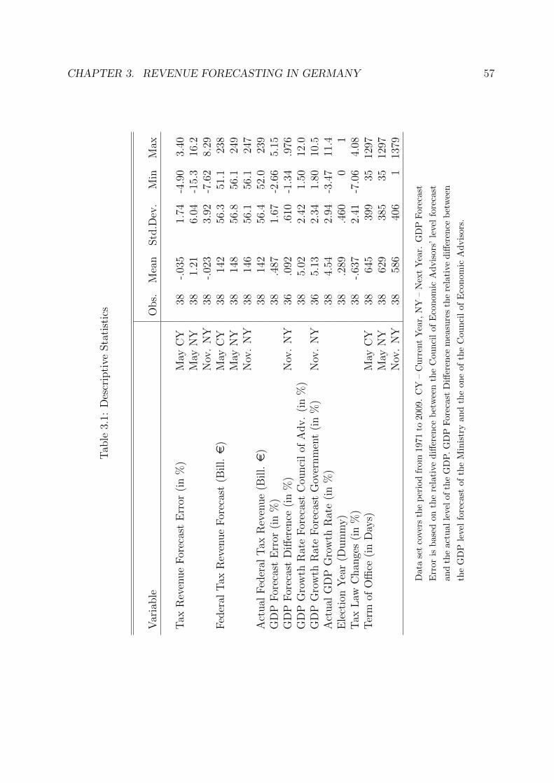
CHAPTER 3. REVENUE FORECASTING IN GERMANY 57
Tab
le3.
1:D
escr
ipti
veSta
tist
ics
Var
iable
Obs.
Mea
nStd
.Dev
.M
inM
ax
Tax
Rev
enue
For
ecas
tE
rror
(in
%)
May
CY
38-.
035
1.74
-4.9
03.
40M
ayN
Y38
1.21
6.04
-15.
316
.2N
ov.
NY
38-.
023
3.92
-7.6
28.
29F
eder
alT
axR
even
ue
For
ecas
t(B
ill.e
)M
ayC
Y38
142
56.3
51.1
238
May
NY
3814
856
.856
.124
9N
ov.
NY
3814
656
.156
.124
7A
ctual
Fed
eral
Tax
Rev
enue
(Bill.e
)38
142
56.4
52.0
239
GD
PF
orec
ast
Err
or(i
n%
)38
.487
1.67
-2.6
65.
15G
DP
For
ecas
tD
iffer
ence
(in
%)
Nov
.N
Y36
.092
.610
-1.3
4.9
76G
DP
Gro
wth
Rat
eF
orec
ast
Cou
nci
lof
Adv.
(in
%)
385.
022.
421.
5012
.0G
DP
Gro
wth
Rat
eF
orec
ast
Gov
ernm
ent
(in
%)
Nov
.N
Y36
5.13
2.34
1.80
10.5
Act
ual
GD
PG
row
thR
ate
(in
%)
384.
542.
94-3
.47
11.4
Ele
ctio
nY
ear
(Dum
my)
38.2
89.4
600
1T
axL
awC
han
ges
(in
%)
38-.
637
2.41
-7.0
64.
08T
erm
ofO
ffice
(in
Day
s)M
ayC
Y38
645
399
3512
97M
ayN
Y38
629
385
3512
97N
ov.
NY
3858
640
61
1379
Dat
ase
tco
vers
the
per
iod
from
1971
to2009.
CY
–C
urr
ent
Yea
r,N
Y–
Nex
tY
ear.
GD
PF
ore
cast
Err
oris
bas
edon
the
rela
tive
diff
eren
ceb
etw
een
the
Cou
nci
lof
Eco
nom
icA
dvis
ors
’le
vel
fore
cast
and
the
actu
alle
vel
ofth
eG
DP
.G
DP
Fore
cast
Diff
eren
cem
easu
res
the
rela
tive
diff
eren
ceb
etw
een
the
GD
Ple
vel
fore
cast
ofth
eM
inis
try
an
dth
eon
eof
the
Cou
nci
lof
Eco
nom
icA
dvis
ors
.

CHAPTER 3. REVENUE FORECASTING IN GERMANY 58
The forecast error that we will focus on is a relative forecast error, i.e. the difference
between the forecasted and the actual revenue divided by the actual revenue. A positive
sign of the forecast error means that the forecast was higher than actual revenue, and a
negative one that it was lower. As Table 3.1 shows, there is an average overestimation of
1.21 percent in next-year forecasts from May, while both other forecasts show a very small
underestimation.
Graphically, the results can be pictured as shown in Figures 3.1 to 3.3. Obviously, the
relative forecast error in next-year forecasts shows a larger amplitude in May than in
November, while the forecast for the current year shows the smallest amplitude. This had
to be expected since a shrinking time span between the preparation of the forecast and
the beginning of the forecasted period lowers the level of uncertainty. In the course of the
years, however, there is no obvious change in the amplitude or the direction of the forecast
error.
Our analysis of the unbiasedness of revenue forecasts is based on three types of variables.
First, to account for the uncertainty of economic circumstances, a measure for the GDP
forecast error is included. This measure is defined as the relative difference between the
independent Council of Economic Advisors’ forecast of the GDP level and the actual level
of the GDP: 100∗(GDP f Advisorst −GDPt)/GDPt.9 Note that this GDP forecast error is not
based on the GDP forecast that underlies the revenue forecast.10 It is rather a GDP forecast
error that measures sheer economic uncertainty and excludes possible political biases of the
underlying official GDP forecast. The latter will come into play in the efficiency analysis
below.
9The GDP forecast of the Council of Economic Advisors is always issued in November, with the resultthat the GDP forecast error represents the level of economic uncertainty always at the same point of time,namely the November prior to the forecasted year, and not at the time where the revenue forecast wasprepared.
10Revenue forecasters are asked to base their forecast on a GDP forecast provided by the Ministry ofEconomics and Technology.

CHAPTER 3. REVENUE FORECASTING IN GERMANY 59
Figure 3.1: Relative Forecast Error (in %): Current-Year Forecast May
−20
−15
−10
−5
05
1015
20R
elat
ive
For
ecas
t Err
or
1970 1975 1980 1985 1990 1995 2000 2005 2010Year
Figure 3.2: Relative Forecast Error (in %): Next-Year Forecast May
−20
−15
−10
−5
05
1015
20R
elat
ive
For
ecas
t Err
or
1970 1975 1980 1985 1990 1995 2000 2005 2010Year

CHAPTER 3. REVENUE FORECASTING IN GERMANY 60
Figure 3.3: Relative Forecast Error (in %): Next-Year Forecast November
−20
−15
−10
−5
05
1015
20R
elat
ive
For
ecas
t Err
or
1970 1975 1980 1985 1990 1995 2000 2005 2010Year
Second, the question of whether the revenue forecast error is changing over time is captured
by trend variables. To allow for nonlinear developments also the squared and cubed forms
of the trend are included. Note that the trend variable is closely related to the level of the
forecast that was part of the regression equations derived in the preceding section. Since
nominal revenues are – by tendency – an increasing function of time, a large value in the
trend variable is associated with a large revenue forecast. Apart from technical reasons for
including the trend, this procedure allows to capture structural changes in the economy,
such as increasing world-economic integration and the German reunification.
Third, we control for different attitudes of ministers, which may be intrinsically opti-
mistic or pessimistic. Accordingly, minister specific effects are included by adding dummy
variables for different ministers of finance. This allows to see whether revenue forecasts
prepared under some ministers show a different performance than those prepared under
others.

CHAPTER 3. REVENUE FORECASTING IN GERMANY 61
To analyze whether the revenue forecasts are efficient, possibly relevant information that
was available at the time where the forecast was made is further taken into account. Among
this is first of all the revenue forecast error from the last period (fet−1).11 It is reasonable
to argue that a forecaster reacts to his last forecast error by adjusting his current forecast
into the opposite direction.
Since the revenue forecasters have to make use of a GDP forecast that is provided by
the Federal Ministry of Economics and Technology it could be that forecast errors arise
from strategic goals. To see whether the revenue forecasts could have been improved
by taking into account other (independent) GDP forecasts, we include a GDP forecast
difference variable. This shows the relative difference between the underlying GDP level
forecast of the Ministry and that of the independent Council of Economic Advisors: 100 ∗
(GDP f Ministryt −GDP f Advisors
t )/GDP f Advisorst .
Another variable concerns tax law changes. Usually, revenue forecasters are asked to
prepare their forecasts based on the current law. Even if a reform proposal will be almost
certainly implemented, it is typically not included in the forecast. But since the law can
pass legislation between the time the forecast is made and the (end of the) forecasted
period, forecast errors may occur that cannot be attributed to the forecaster. To account
for this, a variable measuring the extent of law changes on the total tax level (relative to
total tax revenues) is included.12 But even if tax laws have passed the legislator “in time”,
they can influence the forecast error, since their effects are difficult to assess.13
Incentives can differ when a forecast is prepared for an election year. To take this into
account a dummy variable is included. This takes on the value 1 if the forecast is prepared
for an election year and the value 0 if not.
11Since the forecast error from the previous to the current year is not yet available to the forecaster atthe time of the compilation of the next-year forecasts, this describes the error of the forecast prepared twoperiods ago in the respective cases.
12Indeed, we only analyze federal taxes, but the major tax law changes occurred on this level.
13Note that the estimates of revenue effects of law changes are prepared by the Ministry of Finance.

CHAPTER 3. REVENUE FORECASTING IN GERMANY 62
To investigate whether revenue forecasts are influenced by politics, we further control for
different effects in the course of terms of office. This is done by including a variable
measuring the number of days the government has been in office when a forecast is issued.14
Political incentives right after having been elected might differ from those when the next
election is approaching.
Having discussed the data and the different issues to be addressed, the next section presents
our results of the analyses of unbiasedness, efficiency, and politics.
3.4 Empirical Results
We consider three revenue forecasts and investigate whether they are unbiased, efficient,
and/or influenced by politics: (i) the May forecast for the current year, (ii) the May forecast
for the next year, and (iii) the November forecast for the next year.
Unbiasedness
First, for all three revenue forecasts unbiasedness is considered. In our approach unbiased-
ness requires that neither the constant nor the trend have an impact on the forecast error.
The latter is here defined as the difference between the forecast and the actual tax revenue,
relative to the actual tax revenue.
The upper part of Table 3.2 presents the results for the current-year forecast prepared
in May. While column (1) only includes a constant, in columns (2) to (4) the trend is
added. But irrespective of whether just a linear trend or also nonlinear forms are allowed,
there are no signs of a biased forecast. None of the respective coefficients are significant.
14The term of office ends with federal elections, irrespective of whether the reigning parties remain thesame after the election.

CHAPTER 3. REVENUE FORECASTING IN GERMANY 63
Table 3.2: Results on the Forecast Bias: May current / May next / November next Year
(1) (2) (3) (4) (5) (6) (7) (8) (9) (10)
Constant .001 .213 -.227 .510 2.79 -.205 .073 -.928 -.256 -.136(.278) (.573) (.895) (1.26) (1.71) (.282) (.579) (.953) (1.46) (1.14)
GDP Forecast Error .350 ?? .364 ?? .395 ?? .399 ?? .404 ??
(.164) (.168) (.168) (.169) (.169)Trend -.011 .054 -.154 -.014 .122 -.046
(.025) (.103) (.269) (.025) (.107) (.296)Trend Squared -.002 .011 -.003 .007
(.003) (.015) (.003) (.016)Trend Cubed -.000 -.000
(.000) (.000)Minister Dummies – – – – Yes – – – – Yes
R2 0.000 0.005 0.016 0.036 0.234 0.112 0.120 0.162 0.172 0.349adj. R2 0.000 -0.022 -0.039 -0.047 0.030 0.088 0.070 0.089 0.071 0.169Observations 39 39 39 39 39 38 38 38 38 38
(11) (12) (13) (14) (15) (16) (17) (18) (19) (20)
Constant 1.21 .532 1.36 1.91 4.14 .069 .472 -.189 .970 4.99(.979) (2.10) (3.52) (5.46) (6.62) (.790) (1.63) (2.74) (4.22) (4.44)
GDP Forecast Error 2.34 ??? 2.36 ??? 2.38 ??? 2.39 ??? 3.00 ???
(.460) (.471) (.482) (.489) (.496)Trend .033 -.080 -.216 -.020 .070 -.221
(.090) (.394) (1.11) (.071) (.306) (.855)Trend Squared -.003 .011 -.002 .015
(.009) (.061) (.007) (.047)Trend Cubed -.000 -.000
(.001) (.001)Minister Dummies – – – – Yes – – – – Yes
R2 0.000 0.004 0.006 0.007 0.057 0.418 0.420 0.421 0.424 0.592adj. R2 0.000 -0.024 -0.051 -0.081 -0.204 0.402 0.387 0.370 0.354 0.461Observations 38 38 38 38 38 38 38 38 38 38
(21) (22) (23) (24) (25) (26) (27) (28) (29) (30)
Constant -.023 -.495 .928 -.018 -3.03 -.800 -.536 -.111 -.642 -4.66(.635) (1.36) (2.26) (3.51) (4.27) (.493) (1.02) (1.71) (2.64) (2.81)
GDP Forecast Error 1.59 ??? 1.61 ??? 1.59 ??? 1.59 ??? 1.97 ???
(.287) (.294) (.301) (.305) (.312)Trend .023 -.171 .065 -.013 -.071 .062
(.059) (.253) (.710) (.044) (.191) (.534)Trend Squared -.005 -.009 .001 -.006
(.006) (.039) (.005) (.030)Trend Cubed .000 .000
(.001) (.000)Minister Dummies – – – – Yes – – – – Yes
R2 0.000 0.004 0.022 0.025 0.068 0.461 0.463 0.464 0.465 0.614adj. R2 0.000 -0.023 -0.034 -0.061 -0.189 0.446 0.432 0.417 0.400 0.490Observations 38 38 38 38 38 38 38 38 38 38
Dependent variable: Relative Tax Revenue Forecast Error. Standard errors in parentheses. A single star denotes
significance at the 10 % level, two stars at the 5 % level, and three stars at the 1 % level (in the case of minister
dummies for joint significance).

CHAPTER 3. REVENUE FORECASTING IN GERMANY 64
This also holds when dummy variables for the different ministers of finance are included
in column (5), which in fact prove not to be jointly significant. Columns (6) to (10) repeat
the exercise but in addition the GDP forecast error is included. This variable is defined as
the relative difference between the Council of Economic Advisors’ forecast and the actual
GDP level.15 It shows that this measure of macroeconomic uncertainty is positively related
to the revenue forecast error and it substantially contributes to the level of R2. Since the
GDP forecasts are not made by the revenue forecasters, however, this cannot be considered
as a bias in the revenue forecasts.
When we turn to the forecasts for the next year issued in May and November in columns
(11) to (20) and (21) to (30), these results are confirmed. The GDP forecast error even
contributes more to the coefficients of determination than before. While the regressions
for the May forecast for the current year were only able to explain up to about one third
of the variation of the relative forecast error, the R2 rises to up to 60 % in the case of
next-year forecasts. Comparing the coefficients of the GDP forecast error among the three
revenue forecasts shows the expected magnitudes. Since the GDP forecast error is based
on figures from the November prior to the forecasted year, the coefficients increase with
the time span between the revenue forecast and the beginning of the forecasted period.
Efficiency
Turning to the efficiency of revenue forecasts brings us to the analysis of whether infor-
mation was available at the time of the forecast preparation that could have improved
the quality of the forecasts. Accordingly, none of the respective variables should show a
significant effect for forecasts to be efficient.
15One can alternatively make use of the joint forecast of German research institutes (“Gemeinschafts-diagnose”), rather than of the forecast of the Council of Economic Advisors. The corresponding resultsare comparable and for the next-year forecast from November shown in the appendix.

Table 3.3: Results on Forecast Efficiency I: May current / May next / November next Year
(1) (2) (3) (4)
Constant -.189 .100 .010 .290(.284) (.330) (1.48) (1.16)
lag Revenue Forecast Error .133 .164 .119 -.103(.165) (.162) (.170) (.180)
GDP Forecast Error .309 ? .283 .338 ? .436 ?
(.173) (.170) (.180) (.181)Trend -.032
(.296)Trend Squared .005
(.017)Trend Cubed -.000
(.000)Election Year -.959 -.869 -.830
(.590) (.608) (.574)Minister Dummies – – – Yes
R2 0.129 0.191 0.229 0.407adj. R2 0.079 0.120 0.080 0.188Observations 38 38 38 38
(5) (6) (7) (8)
Constant -.012 .210 1.87 6.07(.856) (.979) (7.00) (4.82)
lag Revenue Forecast Error .040 .053 .047 -.084(.134) (.138) (.147) (.143)
GDP Forecast Error 2.50 ??? 2.52 ??? 2.53 ??? 2.92 ???
(.499) (.505) (.566) (.507)Trend -.305
(1.26)Trend Squared .018
(.065)Trend Cubed -.000
(.001)Election Year -.878 -.747 -.695
(1.81) (1.91) (1.80)Minister Dummies – – – Yes
R2 0.438 0.442 0.448 0.614adj. R2 0.404 0.390 0.334 0.460Observations 36 36 36 36
(9) (10) (11) (12)
Constant -.805 -.605 .703 -4.60 ?
(.512) (.597) (4.25) (2.69)lag Revenue Forecast Error -.011 .001 -.004 -.001
(.133) (.135) (.143) (.139)GDP Forecast Error 1.68 ??? 1.69 ??? 1.65 ??? 1.90 ???
(.308) (.311) (.347) (.297)Trend -.103
(.768)Trend Squared .000
(.039)Trend Cubed .000
(.000)Election Year -.728 -.715 -.606
(1.09) (1.15) (1.00)Minister Dummies – – – Yes ?
R2 0.489 0.496 0.505 0.687adj. R2 0.458 0.449 0.402 0.562Observations 36 36 36 36
Dependent variable: Relative Tax Revenue Forecast Error. Standard errors in parentheses. A
single star denotes significance at the 10 % level, two stars at the 5 % level, and three stars at
the 1 % level (in the case of minister dummies for joint significance).
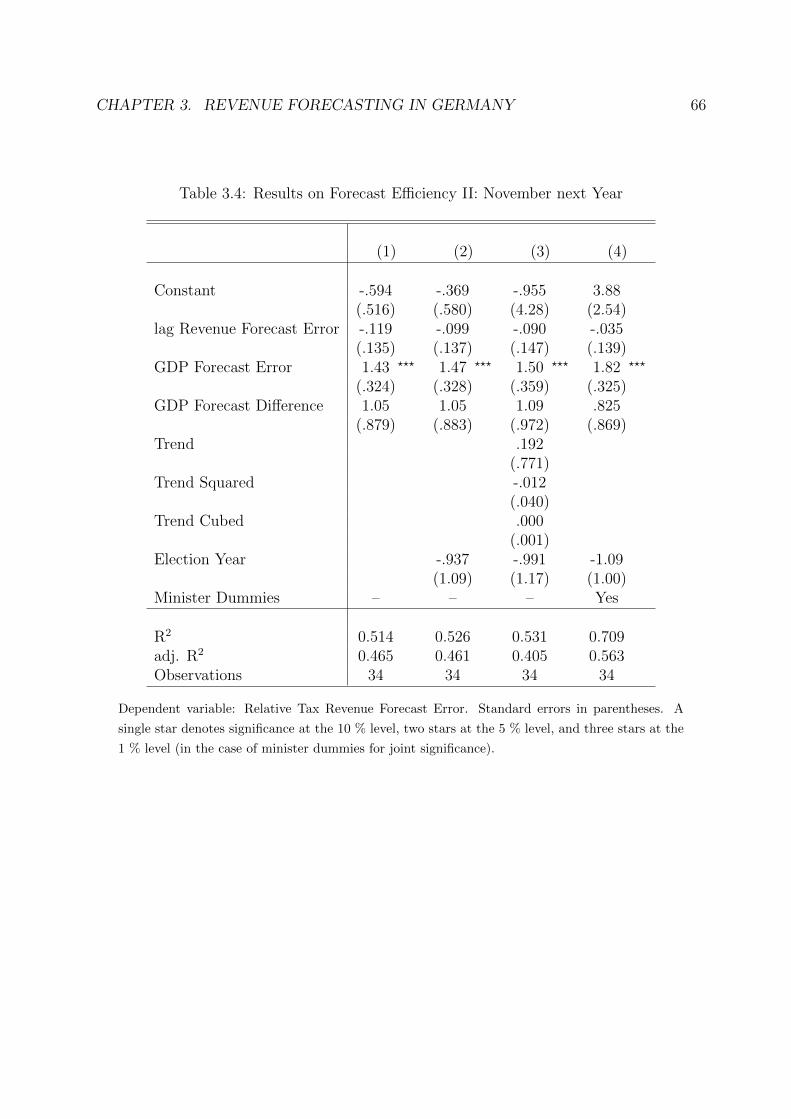
CHAPTER 3. REVENUE FORECASTING IN GERMANY 66
Table 3.4: Results on Forecast Efficiency II: November next Year
(1) (2) (3) (4)
Constant -.594 -.369 -.955 3.88(.516) (.580) (4.28) (2.54)
lag Revenue Forecast Error -.119 -.099 -.090 -.035(.135) (.137) (.147) (.139)
GDP Forecast Error 1.43 ??? 1.47 ??? 1.50 ??? 1.82 ???
(.324) (.328) (.359) (.325)GDP Forecast Difference 1.05 1.05 1.09 .825
(.879) (.883) (.972) (.869)Trend .192
(.771)Trend Squared -.012
(.040)Trend Cubed .000
(.001)Election Year -.937 -.991 -1.09
(1.09) (1.17) (1.00)Minister Dummies – – – Yes
R2 0.514 0.526 0.531 0.709adj. R2 0.465 0.461 0.405 0.563Observations 34 34 34 34
Dependent variable: Relative Tax Revenue Forecast Error. Standard errors in parentheses. A
single star denotes significance at the 10 % level, two stars at the 5 % level, and three stars at the
1 % level (in the case of minister dummies for joint significance).

Table 3.5: Results on Forecast Efficiency III: May current / May next / November nextYear
(1) (2) (3) (4) (5) (6)
Constant -.205 -.084 .140 -.392 -.042 .429(.282) (.279) (.321) (1.02) (1.04) (2.10)
GDP Forecast Error .350 ?? .376 ?? .361 ?? .442 ??? .434 ??? .352 ?
(.164) (.159) (.157) (.151) (.149) (.177)Trend -.431
(.808)Trend Squared .025
(.037)Trend Cubed -.000
(.001)Election Year -.781 -.682
(.572) (.511)Tax Law Changes .211 ? .195 ? .304 ??? .286 ??? .306 ???
(.110) (.109) (.104) (.104) (.109)Minister Dummies – – – Yes ?? Yes ?? Yes ?
R2 0.112 0.197 0.238 0.501 0.532 0.535adj. R2 0.088 0.151 0.171 0.341 0.358 0.312Observations 38 38 38 38 38 38
(7) (8) (9) (10) (11) (12)
Constant .069 -.392 -.232 4.18 5.44 3.04(.790) (.748) (.881) (4.16) (4.49) (6.28)
GDP Forecast Error 2.34 ??? 2.24 ??? 2.23 ??? 2.83 ??? 2.83 ??? 2.71 ???
(.460) (.426) (.432) (.469) (.473) (.471)Trend .714
(2.57)Trend Squared .039
(.115)Trend Cubed -.001
(.002)Election Year -.560 -1.28
(1.57) (1.64)Tax Law Changes -.799 ??? -.810 ?? -.753 ?? -.778 ?? -.948 ??
(.295) (.300) (.334) (.337) (.342)Minister Dummies – – – Yes Yes Yes
R2 0.418 0.520 0.521 0.657 0.665 0.707adj. R2 0.402 0.492 0.479 0.530 0.523 0.548Observations 38 38 38 38 38 38
(13) (14) (15) (16) (17) (18)
Constant -.800 -.976 ? -.855 -4.10 -4.09 -8.71(.493) (.496) (.584) (2.81) (2.84) (15.4)
GDP Forecast Error 1.59 ??? 1.56 ??? 1.55 ??? 1.90 ??? 1.90 ??? 1.90 ???
(.287) (.283) (.287) (.313) (.316) (.336)Trend .562
(1.84)Trend Squared -.006
(.085)Trend Cubed .000
(.001)Election Year -.423 -.718
(1.04) (1.06)Tax Law Changes -.306 -.314 -.290 -.301 -.340
(.196) (.199) (.224) (.227) (.243)Minister Dummies – – – Yes Yes Yes
R2 0.461 0.496 0.499 0.637 0.643 0.647adj. R2 0.446 0.468 0.455 0.502 0.492 0.455Observations 38 38 38 38 38 38
Dependent variable: Relative Tax Revenue Forecast Error. Standard errors in parentheses. A
single star denotes significance at the 10 % level, two stars at the 5 % level, and three stars at
the 1 % level (in the case of minister dummies for joint significance).

CHAPTER 3. REVENUE FORECASTING IN GERMANY 68
We start in Table 3.3 with considering the revenue forecast error from the last available
forecast (lag Revenue Forecast Error). It shows for all forecasts that the hypothesis of
efficiency cannot be rejected at this time. Since the last forecast error does not show an
impact on the current forecast error, we can conclude that this information is taken into
account by the forecaster. Also trend variables do not affect the forecast error; the same
holds for the election year dummy. Again, the GDP forecast error is the only variable with
a significant effect. Only in the case of the next-year forecast from November, there is a
single significant constant and jointly significant minister dummies.
Concerning the November forecast for the next year, we can also add the GDP forecast
difference as a piece of information that was available to the forecaster.16 This GDP forecast
difference measures the (relative) difference between the official GDP forecast that underlies
the revenue forecast and the independent one from the Council of Economic Advisors.
But as Table 3.4 shows, this measure does not significantly affect the revenue forecast
error. Thus, there is no measurable influence of the government via the GDP forecast.
However, the coefficients have the expected positive sign, meaning that revenues tend to be
overestimated when the underlying GDP forecast is more optimistic than the independent
one. The remaining variables show a similar pattern as before. Correspondingly, the
November forecast for the next year still shows no signs of inefficiency.
One factor that shows a significant effect is the variable describing tax law changes. In
the May forecast for the current year, the forecast is based on a widely “correct” legal
situation. Hence, there is hardly any uncertainty left regarding tax law changes in the
forecasted horizon.17 Given that all law changes have already been passed and the fore-
cast is based on the new law, the positive sign in the upper part of Table 3.5 indicates a
too strong assessment of law changes. When a revenue-enhancing law was implemented,
the forecasters expected too positive effects, and when a revenue-reducing law was imple-
16In the cases of the other forecasts this was not possible since respective forecasts are issued only inNovember.
17Tax law changes can also be passed in the course of the year. The argumentation, however, assumesall laws to be passed before May, which is in fact the case for most relevant laws.
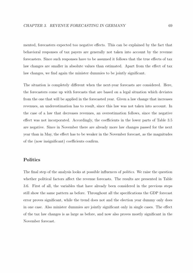
CHAPTER 3. REVENUE FORECASTING IN GERMANY 69
mented, forecasters expected too negative effects. This can be explained by the fact that
behavioral responses of tax payers are generally not taken into account by the revenue
forecasters. Since such responses have to be assumed it follows that the true effects of tax
law changes are smaller in absolute values than estimated. Apart from the effect of tax
law changes, we find again the minister dummies to be jointly significant.
The situation is completely different when the next-year forecasts are considered. Here,
the forecasters come up with forecasts that are based on a legal situation which deviates
from the one that will be applied in the forecasted year. Given a law change that increases
revenues, an underestimation has to result, since this law was not taken into account. In
the case of a law that decreases revenues, an overestimation follows, since the negative
effect was not incorporated. Accordingly, the coefficients in the lower parts of Table 3.5
are negative. Since in November there are already more law changes passed for the next
year than in May, the effect has to be weaker in the November forecast, as the magnitudes
of the (now insignificant) coefficients confirm.
Politics
The final step of the analysis looks at possible influences of politics. We raise the question
whether political factors affect the revenue forecasts. The results are presented in Table
3.6. First of all, the variables that have already been considered in the previous steps
still show the same pattern as before. Throughout all the specifications the GDP forecast
error proves significant, while the trend does not and the election year dummy only does
in one case. Also minister dummies are jointly significant only in single cases. The effect
of the tax law changes is as large as before, and now also proves mostly significant in the
November forecast.
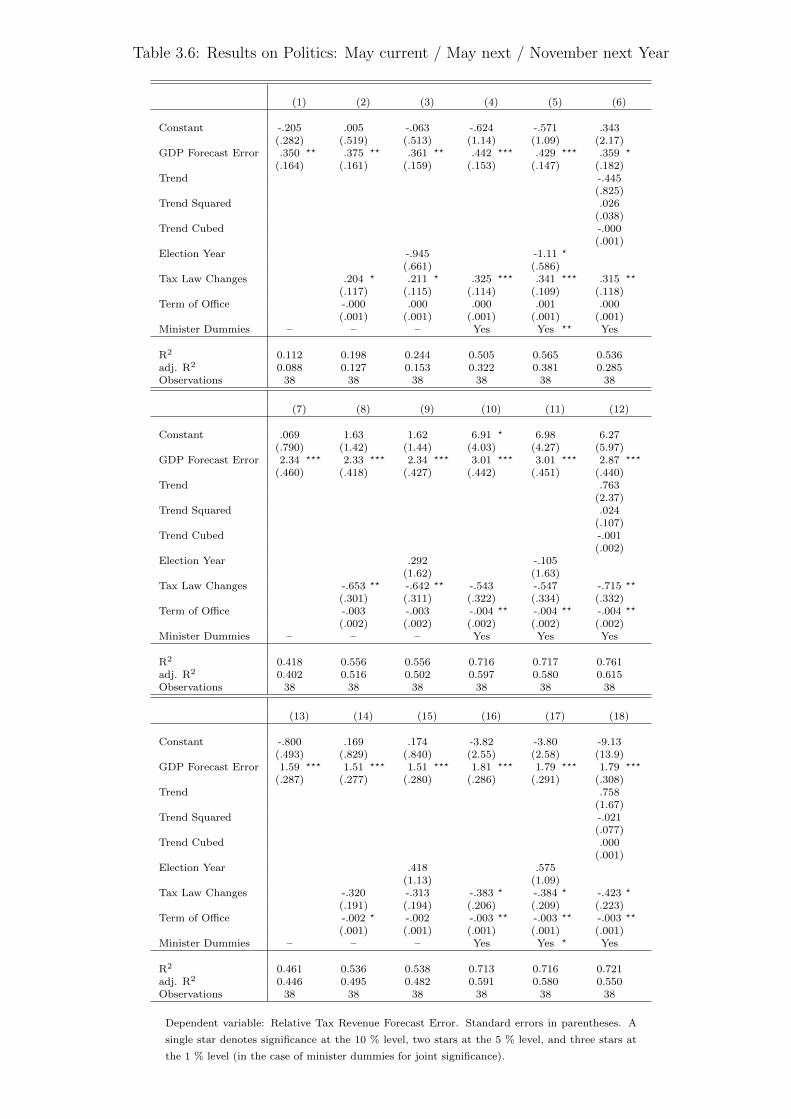
Table 3.6: Results on Politics: May current / May next / November next Year
(1) (2) (3) (4) (5) (6)
Constant -.205 .005 -.063 -.624 -.571 .343(.282) (.519) (.513) (1.14) (1.09) (2.17)
GDP Forecast Error .350 ?? .375 ?? .361 ?? .442 ??? .429 ??? .359 ?
(.164) (.161) (.159) (.153) (.147) (.182)Trend -.445
(.825)Trend Squared .026
(.038)Trend Cubed -.000
(.001)Election Year -.945 -1.11 ?
(.661) (.586)Tax Law Changes .204 ? .211 ? .325 ??? .341 ??? .315 ??
(.117) (.115) (.114) (.109) (.118)Term of Office -.000 .000 .000 .001 .000
(.001) (.001) (.001) (.001) (.001)Minister Dummies – – – Yes Yes ?? Yes
R2 0.112 0.198 0.244 0.505 0.565 0.536adj. R2 0.088 0.127 0.153 0.322 0.381 0.285Observations 38 38 38 38 38 38
(7) (8) (9) (10) (11) (12)
Constant .069 1.63 1.62 6.91 ? 6.98 6.27(.790) (1.42) (1.44) (4.03) (4.27) (5.97)
GDP Forecast Error 2.34 ??? 2.33 ??? 2.34 ??? 3.01 ??? 3.01 ??? 2.87 ???
(.460) (.418) (.427) (.442) (.451) (.440)Trend .763
(2.37)Trend Squared .024
(.107)Trend Cubed -.001
(.002)Election Year .292 -.105
(1.62) (1.63)Tax Law Changes -.653 ?? -.642 ?? -.543 -.547 -.715 ??
(.301) (.311) (.322) (.334) (.332)Term of Office -.003 -.003 -.004 ?? -.004 ?? -.004 ??
(.002) (.002) (.002) (.002) (.002)Minister Dummies – – – Yes Yes Yes
R2 0.418 0.556 0.556 0.716 0.717 0.761adj. R2 0.402 0.516 0.502 0.597 0.580 0.615Observations 38 38 38 38 38 38
(13) (14) (15) (16) (17) (18)
Constant -.800 .169 .174 -3.82 -3.80 -9.13(.493) (.829) (.840) (2.55) (2.58) (13.9)
GDP Forecast Error 1.59 ??? 1.51 ??? 1.51 ??? 1.81 ??? 1.79 ??? 1.79 ???
(.287) (.277) (.280) (.286) (.291) (.308)Trend .758
(1.67)Trend Squared -.021
(.077)Trend Cubed .000
(.001)Election Year .418 .575
(1.13) (1.09)Tax Law Changes -.320 -.313 -.383 ? -.384 ? -.423 ?
(.191) (.194) (.206) (.209) (.223)Term of Office -.002 ? -.002 -.003 ?? -.003 ?? -.003 ??
(.001) (.001) (.001) (.001) (.001)Minister Dummies – – – Yes Yes ? Yes
R2 0.461 0.536 0.538 0.713 0.716 0.721adj. R2 0.446 0.495 0.482 0.591 0.580 0.550Observations 38 38 38 38 38 38
Dependent variable: Relative Tax Revenue Forecast Error. Standard errors in parentheses. A
single star denotes significance at the 10 % level, two stars at the 5 % level, and three stars at
the 1 % level (in the case of minister dummies for joint significance).

CHAPTER 3. REVENUE FORECASTING IN GERMANY 71
The results for the current-year forecast are shown in the upper part of the table. In
addition we now control for the time the government has been in office at the time of the
forecast. However, no effect of the term of office can be found for this forecast.
Turning to the next-year forecasts in May and November displayed in the lower parts of
Table 3.6 provides further insights. When we now control for the duration the government
is in office, we find potential to improve the forecasts. The longer the government is
in office, the smaller the relative forecast error becomes. This is significant throughout
most specifications concerning the next-year forecasts. A possible explanation could be
increasing GDP stimuli by the government at the end of the rule that are not taken into
account by the revenue forecaster and compensate for earlier overestimations.18 However,
because of the coefficients of the election year variable indicating the opposite, this political
business cycle explanation is ruled out. An alternative explanation is that the forecast
error is larger in the beginning of a legislative period, meaning that forecasters provide
more optimistic figures. This could be based on overoptimistic expectations of forecasters
regarding a new government or on pressure of this government to let political programs
appear fundable.19
3.5 Conclusions
This chapter has analyzed the rationality of official revenue forecasts in Germany. Since
these forecasts are essential for the budget process, the Court of Auditors had criticized the
occurrence of overestimation in recent years. We investigate whether evidence for (upward)
biased forecasts can be found, and whether there is room to improve the forecasts in terms
of efficiency.
18See Becker and Buettner (2007).
19The effect of the term of office is weaker and insignificant when total tax revenues rather than onlyfederal ones are considered. Hence, the effect seems to occur only from federal politicians regarding theirown revenues.

CHAPTER 3. REVENUE FORECASTING IN GERMANY 72
Based on the literature on rational forecasting we use the framework developed by Keane
and Runkle to derive regression equations that try to tackle three questions. The first
one concerns unbiasedness of forecasts. A forecast is considered to be unbiased when the
expected value of revenues is consistent with the forecast. The second one asks whether the
forecasts are efficient. This is the case when there was no relevant information available to
the forecaster at the time of the forecast that could have improved the outcome. Finally,
we look at possible influences of politics.
The empirical assessment focuses on the spring forecasts for the current and the next year
as well as on the fall forecast for the next year. Employing data for federal tax revenues
covering the period from 1971 to 2009 we are able to widely “acquit” the forecasters.
The analysis concerning unbiasedness shows that the hypothesis of unbiasedness cannot
be rejected. For none of the three forecasts there are signs for biasedness. Rather the
GDP forecast error explains a notable part of the revenue forecast error. Turning to the
question of efficiency yields to including some pieces of information that appear to have
a possible impact on the forecast error. Neither the last revenue forecast error, nor the
difference between the official and an independent GDP forecast, nor a dummy variable
for election years shows any significance. However, we find the estimated effects of tax
law changes to be too strong, when they are taken into account. If, however, they have
been passed by the legislator after the preparation of the forecast, the expected effects of
over- or underestimation are found. Moreover, the GDP forecast error still proves relevant.
Considering variables describing political circumstances we find some room to improve the
forecasts; the forecast error is affected by the term of office. The longer the government is
in office, the smaller the forecast error becomes. This might reflect larger overestimations
at the beginning of the rule, either because forecasters are overoptimistic regarding a new
government, or due to political pressure to convey the impression that political programs
are sufficiently funded.

CHAPTER 3. REVENUE FORECASTING IN GERMANY 73
Appendix
Table 3.7: Results on the Forecast Bias: November Forecast for the next Year (GDPForecast Error based on Research Institutes)
(1) (2) (3) (4) (5)
Constant -.023 -.495 .928 -.018 -3.03(.635) (1.36) (2.26) (3.51) (4.27)
GDP Forecast Error
Trend .023 -.171 .065(.059) (.253) (.710)
Trend Squared -.005 -.009(.006) (.039)
Trend Cubed .000(.001)
Minister Dummies – – – – Yes
R2 0.000 0.004 0.022 0.025 0.068adj. R2 0.000 -0.023 -0.034 -0.061 -0.189Observations 38 38 38 38 38
(6) (7) (8) (9) (10)
Constant -.855 ? -.493 -.305 -.932 -4.84 ?
(.465) (9.55) (1.62) (2.49) (2.59)GDP Forecast Error 1.53 ??? 1.55 ??? 1.54 ??? 1.54 ??? 1.85 ???
(.244) (.250) (.257) (.261) (.258)Trend -.018 -.044 .113
(.042) (.181) (.503)Trend Squared .001 -.009
(.004) (.028)Trend Cubed .000
(.000)Minister Dummies – – – – Yes
R2 0.521 0.524 0.524 0.526 0.672adj. R2 0.508 0.497 0.482 0.468 0.566Observations 38 38 38 38 38
Dependent variable: Relative Tax Revenue Forecast Error. Standard errors in parentheses. A single star denotes
significance at the 10 % level, two stars at the 5 % level, and three stars at the 1 % level (in the case of minister
dummies for joint significance).

CHAPTER 3. REVENUE FORECASTING IN GERMANY 74
Table 3.8: Results on Forecast Efficiency I: November Forecast for the next Year (GDPForecast Error based on Research Institutes)
(1) (2) (3) (4)
Constant -.880 ? -.681 -1.56 3.72(.493) (.574) (4.22) (2.54)
lag Revenue Forecast Error .037 .049 .057 .102(.129) (.131) (.140) (.135)
GDP Forecast Error 1.60 ??? 1.61 ??? 1.64 ??? 1.82 ???
(.269) (.271) (.314) (.262)Trend .275
(.757)Trend Squared -.017
(.039)Trend Cubed .000
(.001)Election Year -.726 -.773 -.742
(1.05) (1.11) (.953)Minister Dummies Yes ??
R2 0.531 0.537 0.545 0.717adj. R2 0.502 0.494 0.450 0.604Observations 36 36 36 36
Dependent variable: Relative Tax Revenue Forecast Error. Standard errors in parentheses. A single star denotes
significance at the 10 % level, two stars at the 5 % level, and three stars at the 1 % level (in the case of minister
dummies for joint significance).

CHAPTER 3. REVENUE FORECASTING IN GERMANY 75
Table 3.9: Results on Forecast Efficiency II: November Forecast for the next Year (GDPForecast Error based on Research Institutes)
(1) (2) (3) (4)
Constant -.593 -.396 -1.36 3.76(.512) (.580) (4.20) (2.55)
lag Revenue Forecast Error -.080 -.069 -.059 .014(.145) (.147) (.157) (.152)
GDP Forecast Error 1.43 ??? 1.44 ??? 1.49 ??? 1.71 ???
(.278) (.281) (.324) (.280)GDP Forecast Difference .454 .603 .629 .663
(1.20) (1.22) (1.29) (1.13)Trend .248
(.758)Trend Squared -.014
(.039)Trend Cubed .000
(.001)Election Year -.817 -.874 -.974
(1.09) (1.18) (1.02)Minister Dummies Yes
R2 0.521 0.530 0.536 0.707adj. R2 0.473 0.465 0.411 0.560Observations 34 34 34 34
Dependent variable: Relative Tax Revenue Forecast Error. Standard errors in parentheses. A single star denotes
significance at the 10 % level, two stars at the 5 % level, and three stars at the 1 % level (in the case of minister
dummies for joint significance). The GDP Forecast Difference is based on the forecasts of the government and the
research institutes.

CHAPTER 3. REVENUE FORECASTING IN GERMANY 76
Table 3.10: Results on Forecast Efficiency III: November Forecast for the next Year (GDPForecast Error based on Research Institutes)
(1) (2) (3) (4) (5) (6)
Constant -.855 ? -.974 ?? -.859 -4.40 -4.38 -7.69(.465) (.473) (.557) (2.62) (2.64) (14.4)
GDP Forecast Error 1.53 ??? 1.49 ??? 1.48 ??? 1.80 ??? 1.80 ??? 1.78 ???
(.244) (.246) (.249) (.263) (.266) (.282)Trend .361
(1.72)Trend Squared -.003
(.079)Trend Cubed -.000
(.001)Election Year -.400 -.690
(.996) (.983)Tax Law Changes -.225 -.233 -.221 -.232 -.258
(.188) (.192) (.211) (.213) (.230)Minister Dummies – – – Yes Yes Yes
R2 0.521 0.540 0.542 0.685 0.691 0.690adj. R2 0.508 0.514 0.502 0.568 0.560 0.522Observations 38 38 38 38 38 38
Dependent variable: Relative Tax Revenue Forecast Error. Standard errors in parentheses. A single star denotes
significance at the 10 % level, two stars at the 5 % level, and three stars at the 1 % level (in the case of minister
dummies for joint significance).

CHAPTER 3. REVENUE FORECASTING IN GERMANY 77
Table 3.11: Results on Politics: November Forecast for the next Year (GDP Forecast Errorbased on Research Institutes)
(1) (2) (3) (4) (5) (6)
Constant -.855 ? .144 .150 -4.11 ? -4.09 ? -8.20(.465) (.790) (.800) (2.30) (2.33) (12.6)
GDP Forecast Error 1.53 ??? 1.44 ??? 1.44 ??? 1.72 ??? 1.71 ??? 1.70 ???
(.244) (.240) (.243) (.232) (.236) (.249)Trend .592
(1.51)Trend Squared -.019
(.070)Trend Cubed .000
(.001)Election Year .425 .652
(1.08) (.978)Tax Law Changes -.241 -.234 -.318 -.319 -.346
(.183) (.187) (.188) (.190) (.203)Term of Office -.002 ? -.002 ? -.003 ??? -.003 ??? -.003 ???
(.001) (.001) (.001) (.001) (.001)Minister Dummies – – – Yes ?? Yes ?? Yes ??
R2 0.521 0.578 0.580 0.766 0.770 0.772adj. R2 0.508 0.541 0.529 0.667 0.660 0.633Observations 38 38 38 38 38 38
Dependent variable: Relative Tax Revenue Forecast Error. Standard errors in parentheses. A single star denotes
significance at the 10 % level, two stars at the 5 % level, and three stars at the 1 % level (in the case of minister
dummies for joint significance).

CHAPTER 3. REVENUE FORECASTING IN GERMANY 78
References
Auerbach, A. J. (1996): Dynamic Revenue Estimation, Journal of Economic Perspectives,
10 (1), 141–157.
Becker, I. and T. Buettner (2007): Are German Tax-Revenue Forecasts Flawed?, unpub-
lished manuscript.
Buettner, T. and G. A. Horn (1993): Wie gut sind Prognosen? Eine Uberprufung der
Vorhersagen der Gemeinschaftsdiagnose und des DIW am Beispiel des BSP, Diskus-
sionspapier DIW, 73.
Buettner, T. and B. Kauder (2010): Revenue Forecasting Practices: Differences across
Countries and Consequences for Forecasting Performance, Fiscal Studies, 31 (3),
313–340.
Feenberg, D. R., W. Gentry, D. Gilroy, and H. S. Rosen (1989): Testing the Rationality
of State Revenue Forecasts, Review of Economics and Statistics, 71 (2), 300–308.
Gebhardt, H. (2001): Methoden, Probleme und Ergebnisse der Steuerschatzung, RWI-
Mitteilungen 2001, 127–147.
Keane, M. D. and D. E. Runkle (1989): Are Economic Forecasts Rational? Quarterly
Review of the Federal Reserve Bank of Minneapolis, 13.
Keane, M. D. and D. E. Runkle (1990): Testing the Rationality of Price Forecasts: New
Evidence from Panel Data, American Economic Review, 80 (4), 714–735.
Laster, D., P. Bennett, and I. S. Geoum (1999): Rational Bias in Macroeconomic Fore-
casts, Quarterly Journal of Economics, 114 (1), 293–318.
McNees, S. K. (1978): The “Rationality” of Economic Forecasts, American Economic
Review, 68 (2), 301–305.

CHAPTER 3. REVENUE FORECASTING IN GERMANY 79
Nordhaus, W. D. (1987): Forecasting Efficiency: Concepts and Applications, Review of
Economics and Statistics, 69, 667–674.

Chapter 4
Spatial Administrative Structure and
Inner-Metropolitan Tax Competition

CHAPTER 4. INNER-METROPOLITAN TAX COMPETITION 81
Abstract
This chapter considers the impact of the shape of municipalities’ borders on local business
tax policy. First, a model is presented that shows the dependence of the level of taxation
on the spatial administrative structure. Afterwards, data from Germany are employed to
discover the effects of the number and size of municipalities within agglomerations. In
the definition of agglomerations we rely on the one hand on a distance-based approach,
but further develop a method that is based on cumulative population densities. The
results show that the spatial administrative structure matters for the level of local business
taxation. On the one hand, the core city’s tax rate in a metropolitan area is lower the
more municipalities are situated around the city. The effect is confirmed when we focus on
the average population size of neighboring municipalities rather than on the sheer number
of them. On the other hand, the tax of the core city is higher the larger its population
share in the agglomeration. Thereby, the result has more power for regions which are more
widely defined. These empirical results coincide with those results from the theoretical
analysis.
4.1 Introduction
Analyzing the role of borders has always been an important research topic in economics,
not only since the significant increase in global trade in recent years and decades. Typically,
the questions being discussed deal with the trade of goods and services between countries.
The literature has found a notable impact of borders on the intensity of trade between
regions. Helliwell (1997) for instance has shown, that trade between provinces of Canada
is much more intensive than trade between these provinces and states of the U.S. Borders
do not just impose a restriction on the intensity of trade, however, they also define the
number of players in the competition of institutions. This chapter aims to look at a smaller
administrative level than states, namely metropolitan areas. Within this context, borders
have also been widely subject to empirical analyses. Hoxby (2000) studied the impact

CHAPTER 4. INNER-METROPOLITAN TAX COMPETITION 82
of the concentration of public school districts in metropolitan areas on school outcomes,
where rivers acting as natural borders serve as an instrument for concentration. She found
a positive effect of the number of school districts on the quality of schooling. Even closer
to the main issue of this chapter is the study of Hatfield and Kosec (2009). They examine
the administrative structure of metropolitan statistical areas in the U.S. and their impacts
on income growth. They find the latter to be higher in areas that host many county
governments.
From this regional perspective borders are the crucial determinant of the scope of local
governments’ actions. They define which firms are subject to taxation, to fees for public
services, but also the area of authority of public administration in general. However, one
cannot assume that borders have been designed mainly according to economic considera-
tions. While in rare cases borders follow natural conditions, as in the case of islands, in
most cases their design is accompanied by a certain degree of arbitrariness. This holds
in particular for agglomerations. While the arbitrariness in cases of clear-cut villages is
not of major importance, as long as all inhabitants of the settlement are covered by the
village area, the situation proves different when borders cut populations. When this is the
case, the location of business can be strongly driven by borders. Firms that decided not to
locate their business in the core of the city, but rather at the border, can choose between
two or more municipalities, which makes them subject to different administrative bodies.
Given that the proximity to customers or relevant public infrastructure is the same at both
sides of the border, the firm will choose the municipality that provides a more appealing
bundle of taxes and administrative services. When it is assumed that the core of a city is
naturally more attractive to firms (as long as we keep public policy issues to one side), tax
competition should be the fiercer the closer the border of a city is drawn around its core,
since then the surrounding municipality can also participate in the core’s benefits (such
as the higher density of consumers). With a wide border, however, the city can tax its

CHAPTER 4. INNER-METROPOLITAN TAX COMPETITION 83
(exclusive) benefits of agglomeration away, which means less tax competition.1
In this chapter we analyze the extent to which municipal borders exert effects on local
business taxation, relying on German data. Since the population density of Germany is
rather high, there is a notable number of agglomerations2 that are characterized by a
settlement that crosses borders. The arbitrariness of municipal borders mentioned above
compels us to take a closer look at the influences of borders on local policy. Since the local
business tax (“Gewerbesteuer”) is one of the most effective economic measures employed
by local politicians it is the impact of the borders’ design on this instrument that seems
to be particularly relevant. Due to the fact that German municipalities have a high degree
of freedom with respect to choosing their local rate of business taxation, it is of interest
to see in which way the policy of highly segmented metropolitan areas differs from that of
those regions that consist only of a few municipalities. Apart from the sheer number of
municipalities, the population share of the city in its agglomeration is another indicator of
potential importance in this context. In fact, it turns out that both the segmentation of
the region and the share of the city are important covariates in explaining the city’s level
of taxation. This holds for two different approaches to define regions – one that is based
on distances and another that relies on cumulative population densities. The analysis
could eventually allow to infer changes in tax policy that could follow after reforms of the
borderlines. In doing so, however, the impacts on the city and those on the region would
have to be distinguished.
The chapter is organized as follows: The next section presents results from a theoretical
model, Section 4.3 provides some background information on German municipalities and
institutions. While Section 4.4 describes the definition of agglomerations and the empirical
strategy, Section 4.5 shows the results. Section 4.6 concludes.
1See Buettner and Kauder (2010) for an analysis of the locational competition between city and sur-rounding area in the case of Frankfurt, with the focus on the local business tax.
2Note that the terms “agglomeration”, “metropolitan area”, and “region” are used interchangeably inthe following.

CHAPTER 4. INNER-METROPOLITAN TAX COMPETITION 84
4.2 Theoretical Model
To analyze the impacts of different administrative structures we start by considering a theo-
retical model.3 Here, the analysis follows the framework of the standard tax-competition
model established by Zodrow and Mieszkowski (1986).
We consider a region that consists of i = 1, 2, ..., n municipalities, where one municipality
is the core city, and the others form the surrounding area. In municipality i there are Li
households, each providing one unit of labor. Firms produce a single good with a linear
homogenous production function F i(Ki, Li), where Ki denotes capital.4 We assume capital
to be perfectly mobile, so that the marginal product of capital equals the rate of return r.
Since all municipalities face the same rate of return in equilibrium, we can write:
F iK(Ki, Li) = r.
Household income consists of both labor (wLi, where w denotes the wage rate) and capital
income (rsi, with si denoting savings). Their utility depends on private consumption xi
and public good consumption zi.
To finance public goods, the government raises a distortionary tax on capital, τ i. Hence,
the government budget constraint reads
τ iKi = zi,
where the costs of providing public goods are assumed to equal their size, zi.5
3In the following we will use the term administrative structure as the short form of spatial administrativestructure.
4This implies: F (K,L) = FKK + FLL. Furthermore, we assume: ∂F∂K ≡ FK > 0, ∂F
∂L ≡ FL > 0,∂2F∂K2 ≡ FKK < 0, ∂2F
∂L2 ≡ FLL < 0, ∂2F∂K∂L ≡ FKL > 0, and ∂3F
∂K2∂L ≡ FKKL > 0.
5In reality there is typically also a residence-based capital tax. This, however, can be neglected here,
CHAPTER 4. INNER-METROPOLITAN TAX COMPETITION 85
Each firm will maximize its profits
πi = F i(Ki, Li)− (r + τ i)Ki − wLi,
that consist of output net of costs of capital (including taxes) and labor.6 The resulting
first-order conditions are
F iK = r + τ i (4.1)
and
F iL = w.
Differentiating (4.1) yields:
F iKK∂K
i =∂r
∂τ i∂τ i + ∂τ i.
Arranging this equation yields the effect of a tax increase in i on the capital employed in
i:∂Ki
∂τ i=
∂r∂τ i
+ 1
F iKK
. (4.2)
Following an analogous procedure, the impact of a tax increase in i on the capital in j
reads:∂Kj
∂τ i=
∂r∂τ i
F jKK
. (4.3)
In equilibrium, the employed capital in all municipalities equals the total amount of capital
in the region:7
Ki +n∑j 6=i
Kj = K.
since it is – in Germany – determined at the national level.
6Here, the firm’s profits are independent of the level of public goods. The assumption is that publicgoods exert perfect spillovers for firms, so that the benefit from them is everywhere the same within anagglomeration. Then firms are just sensitive to tax rates, and not to public goods.
7Since differences in the administrative structure may result in high tax and low tax regions, one couldconsider the total amount of capital in the region to depend on the level of taxation. We neglect suchinterregional aspects in the following, since our focus is on intraregional aspects.

CHAPTER 4. INNER-METROPOLITAN TAX COMPETITION 86
Differentiating this with respect to τ i yields:
∂Ki
∂τ i+
n∑j 6=i
∂Kj
∂τ i= 0.
Since all municipalities (apart from the core) are symmetric, and assuming i to be the
core, this can be simplified to:
∂Ki
∂τ i+ (n− 1)
∂Kj
∂τ i= 0.
Using (4.2) and (4.3) yields:
∂r∂τ i
+ 1
F iKK
+ (n− 1)∂r∂τ i
F jKK
= 0. (4.4)
In contrast to the original framework by Zodrow and Mieszkowski, here the second deriva-
tives of the production function with respect to capital do not cancel. Because the city can
have a higher capital stock (and more labor) than the other municipalities, these deriva-
tives may differ, even though the marginal products of capital have to be the same in
equilibrium.
Before we can find out about the effects of different administrative structures, we have
to solve the municipal-government problem. The benevolent mayor will maximize the
utility of the representative private household. Since private consumption can be written
as ci = F i(Ki)−F iKK
i+rsiLi and the public good as zi = τ iKi, the maximization problem
reads:
maxτ i ui(F i(Ki)− F i
KKi + rsiLi, τ iKi).
The FOC then becomes:
uic(−F iKK
∂Ki
∂τ iKi +
∂r
∂τ isiLi) + uiz(K
i + τ i∂Ki
∂τ i) = 0.

CHAPTER 4. INNER-METROPOLITAN TAX COMPETITION 87
Given a balanced capital account (siLi = Ki) and using (4.2) this can be rearranged to
uizuic
=Ki
Ki + τ i ∂Ki
∂τ i
, (4.5)
which is the marginal cost of public funds (MCPF).
Proposition 1. When the core city faces (n− 1) competitors, the chosen tax rate in the
core will be declining in n. Hence, the level of underprovision of public goods is increasing
in the number of municipalities.
Proof: Solving equation (4.4) for ∂r∂τ i
yields:
∂r
∂τ i= − 1
1 + (n− 1)F iKK
F jKK
. (4.6)
Differentiating this with respect to the number of municipalities n yields:
∂ ∂r∂τ i
∂n=
F iKK
F jKK
(1 + (n− 1)F iKK
F jKK
)2> 0.
Hence, the effect of a tax increase on the return to capital r becomes less negative when
the number of municipalities is rising. Plugging this into (4.2), the RHS of that becomes
more negative and the MCPF (4.5) increases. Thus, the underprovision of public goods
becomes more severe and the tax rate is declining.
Proposition 2. The core city will set a tax rate that is higher, the larger the core city’s
share of total labor in the region.
Proof: Starting from (4.6), the impact of an increase in the share of labor of the core city

CHAPTER 4. INNER-METROPOLITAN TAX COMPETITION 88
(Li
L), holding everything else constant, becomes:
∂ ∂r∂τ i
∂ Li
L
=(n− 1)
∂FiKK
FjKK
∂ Li
L
(1 + (n− 1)F iKK
F jKK
)2< 0.
Since the derivative in the numerator is negative, the impact of a tax increase on the
return to capital will be stronger (more negative) when the labor share of the city is
higher. Plugging this into (4.2) yields a smaller impact of a tax increase on the stock of
capital in the core. Accordingly, the MCPF (4.5) will approach one from above when the
labor share of the core increases. Hence, there will be less underprovision of public goods
and therefore a higher tax rate in the core when its share of total labor is larger.
4.3 German Municipalities and Institutions
Having shown the results that are predicted by standard tax-competition theory, we try
to test whether they can be confirmed in an empirical analysis. In doing so we rely on
German data from 2007. First, it is reasonable to have a look at the German institutions,
since their design might influence the results.
The tax system in Germany allows both the Federal Government and the municipalities to
tax business income. While municipalities take the rate of the corporate tax as given, they
decide upon the rate of the local business tax. To be chosen is the “rate of assessment”,
which has a lower bound of 200 points but no upper bound. Since this rate currently
is multiplied by 3.5 % to obtain the percentage being taxed away, it equals a minimal
burden of 7 %. The lower bound was introduced in 2004 to avoid zero-tax strategies in

CHAPTER 4. INNER-METROPOLITAN TAX COMPETITION 89
single municipalities.8 The highest rate in 2007 was 490 points (in the city of Munich, for
example).9 The local business tax is the most important autonomously determined source
of revenue for German municipalities. In the average city it generated about 52 % of tax
revenues in 2007 (see Figure 1.2).
Altogether there were 12263 municipalities in Germany in 2007. The trend of recent years
shows a notable decline in the number of municipalities in eastern Germany, while the
figure is rather constant in other parts of the country.10 There are significant differences
in the municipal structure among the German states (“Bundeslander”), as can be seen in
Figure 4.1. Here, the number of municipalities per 100 square kilometers is shown. The
state of Rhineland-Palatinate, for instance, comprises 2306 municipalities but the state of
North Rhine-Westphalia just 396, though the latter is characterized by a larger area. This
indicates a high degree of variation in the data used.
A data set with all German municipalities is employed, where information on the popula-
tion, the area, the local business tax rate and some further derived measures is exploited.
To measure the (linear) distance between municipalities, we rely on the geographical co-
ordinates of their official central points. The latter are well-defined in Germany and are
typically some very central places in the centers of the municipalities.
8The municipality of Norderfriedrichskoog (about 40 inhabitants) in northern Germany had attractedsome hundred firms until 2004 with a zero tax rate. The lower bound aims at preventing the emergenceof such tax havens with phantom companies.
9To be precise, three municipalities charged an even higher rate, but all of them have less than 100inhabitants. The “number one” was Dierfeld (8 inhabitants) with a rate of 900.
10Compare Chapter 5.
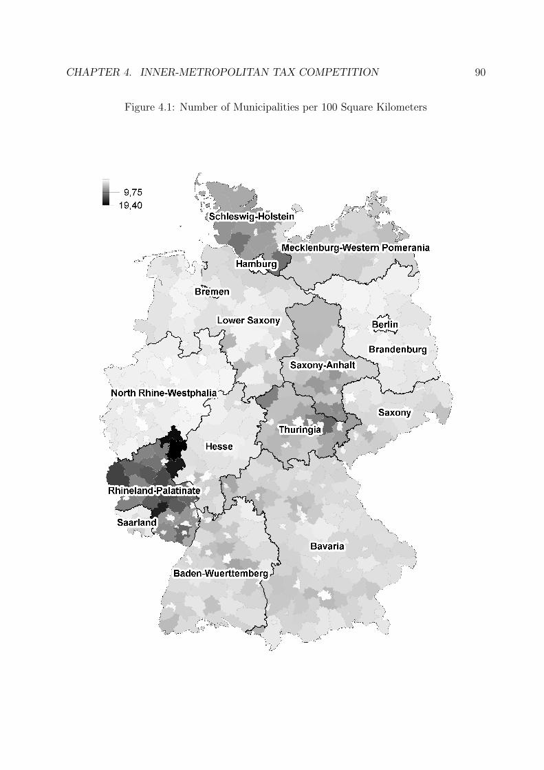
CHAPTER 4. INNER-METROPOLITAN TAX COMPETITION 90
Figure 4.1: Number of Municipalities per 100 Square Kilometers

CHAPTER 4. INNER-METROPOLITAN TAX COMPETITION 91
4.4 Agglomerations and Empirical Strategy
We seek to explain the local business tax rate of the core city of an agglomeration. To
identify differences in tax policies among cities as a function of the administrative structure
we have to give some thought to how agglomerations can be defined and for which cities
this should be done. The answer to the second question is that we will define agglo-
merations around all cities that are independent of counties (“Kreisfreie Stadte”).11 In
2007 there existed 118 of these cities. Since this status typically correlates with size, the
units considered comprise most of Germany’s large cities.12
To answer the first question concerning how agglomerations can be defined, one needs to
engage in some more fundamental thinking. Obviously, there exists no universal definition
of agglomerations. The United Nations defines urban agglomerations as “the de facto
population contained within the contours of a contiguous territory inhabited at urban
density levels without regard to administrative boundaries. It usually incorporates the
population in a city or town plus that in the sub-urban areas lying outside of but being
adjacent to the city boundaries.” While this definition obviously focuses on population
densities and a pretty narrow geographical expanse, the UN definition of metropolitan
areas also focuses on economic links and captures a broader area. According to this, a
metropolitan area “includes both the contiguous territory inhabited at urban levels of
residential density and additional surrounding areas of lower settlement density that are
also under the direct influence of the city (e.g., through frequent transport, road linkages,
commuting facilities etc.).”13
11These cities are not associated with a county, but are directly subordinate to their state. In contrast,a county-dependent city is part of a county, which is at an intermediate stage between city and state.
12The cities of Hanover and Saarbrucken are also considered “Kreisfreie Stadte”, even though their legalstatus deviates slightly (“Kommunalverband besonderer Art”).
13See the UN website: http://esa.un.org/wup2009/unup/index.asp?panel=6.

CHAPTER 4. INNER-METROPOLITAN TAX COMPETITION 92
Since these two definitions, with the first being a subset of the second, underpin the diffi-
culties in finding an appropriate definition of agglomerations, we will employ two different
approaches. These try to capture the different aspects stated by the UN. While our first ap-
proach is based on the sheer proximity of municipalities to a core city, our second approach
covers the idea of focusing on population densities.
The first approach defines an agglomeration as consisting of all municipalities that have
their central point within a certain distance (of 15, 25, or 50 km) to the core city (see
Figure 4.2). In contrast, the second approach sorts the surrounding municipalities precisely
according to their distance to the core. Starting from the core, we add municipalities
– with increasing distances – until the cumulative population density from the core to
the respective municipality no longer changes significantly. The resulting area is then
considered the agglomeration (see Figure 4.3; a more detailed explanation follows below).
It has to be emphasized that agglomerations’ size differs from city to city in the second
approach, while it is the same for all cities in the first approach. In both approaches it can
happen that agglomerations overlap.14
To describe the different structures within agglomerations, we establish basically two kinds
of indicators: the position of the core city relative to the surrounding municipalities on
the one hand, and the picture of the surrounding municipalities among themselves on the
other hand. Accordingly, as the first independent variable the population of the core city
relative to the total population in the agglomeration is calculated. This “share of core”
aims at measuring the “power” of the core in the region. Table 4.1 displays the ten largest
14As an alternative approach, also the so-called “BIK regions” have been considered. The concept ofBIK regions (provided by BIK ASCHPURWIS+BEHRENS ) is based on Boustedt (1953), who in turntook the US concept of “Standard Metropolitan Areas” (SMA) as a model. According to the BIK-regionsconcept agglomerations are formed by those surrounding municipalities in which a certain share of thepopulation is commuting to the core city. Thus, it is pretty close to the UN definition of metropolitanareas. Since the empirical results with this approach are both qualitatively and quantitatively comparableto those in the two other approaches, we do not present these results.

CHAPTER 4. INNER-METROPOLITAN TAX COMPETITION 93
Figure 4.2: The Definition of Agglomerations (First Approach)
In the first approach all municipalities that have
their central points within a certain distance to
the core are part of the region and are here il-
lustrated by shadowed areas and a circle. The
agglomeration shown here comprises six munici-
palities plus the core.
German cities and the population shares in their agglomerations, defined with a radius of
50 km around the city, respectively.
To measure the intensity of competition the city is exposed to, we consider two alternative
variables: On the one hand we look at the sheer number of municipalities within the
region. On the other hand, the average population of the surrounding municipalities is
used, whereby the size of the neighboring municipalities is typically negatively correlated
with their number.
In this context, it seems reasonable to assume that close-to-the-core municipalities play
a different role than those that are located farther away.15 The consideration of regions
defined with different radii aims at capturing this. The larger the region we are looking
at, the smaller we expect the impact of the fragmentation on the level of taxation in the
core to be.
15For an analysis of the role of different locations of administrative bodies in the case of commodity taxcompetition, see Ohsawa (1999).
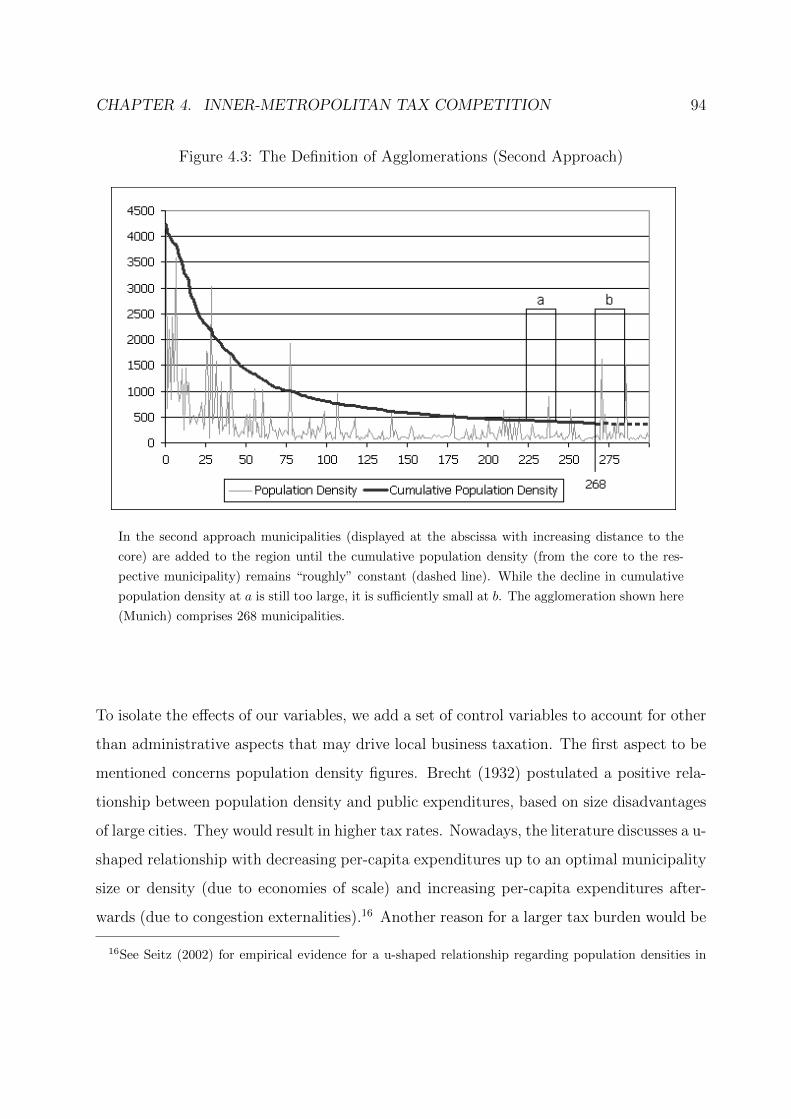
CHAPTER 4. INNER-METROPOLITAN TAX COMPETITION 94
Figure 4.3: The Definition of Agglomerations (Second Approach)
In the second approach municipalities (displayed at the abscissa with increasing distance to the
core) are added to the region until the cumulative population density (from the core to the res-
pective municipality) remains “roughly” constant (dashed line). While the decline in cumulative
population density at a is still too large, it is sufficiently small at b. The agglomeration shown here
(Munich) comprises 268 municipalities.
To isolate the effects of our variables, we add a set of control variables to account for other
than administrative aspects that may drive local business taxation. The first aspect to be
mentioned concerns population density figures. Brecht (1932) postulated a positive rela-
tionship between population density and public expenditures, based on size disadvantages
of large cities. They would result in higher tax rates. Nowadays, the literature discusses a u-
shaped relationship with decreasing per-capita expenditures up to an optimal municipality
size or density (due to economies of scale) and increasing per-capita expenditures after-
wards (due to congestion externalities).16 Another reason for a larger tax burden would be
16See Seitz (2002) for empirical evidence for a u-shaped relationship regarding population densities in
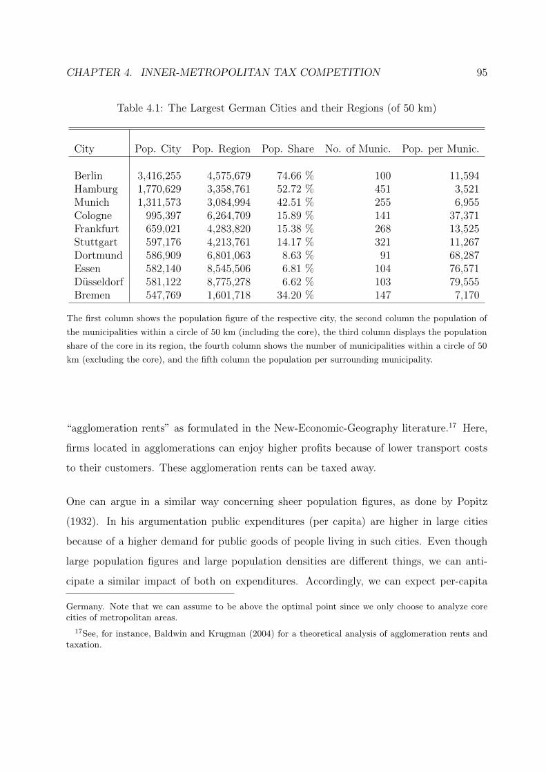
CHAPTER 4. INNER-METROPOLITAN TAX COMPETITION 95
Table 4.1: The Largest German Cities and their Regions (of 50 km)
City Pop. City Pop. Region Pop. Share No. of Munic. Pop. per Munic.
Berlin 3,416,255 4,575,679 74.66 % 100 11,594Hamburg 1,770,629 3,358,761 52.72 % 451 3,521Munich 1,311,573 3,084,994 42.51 % 255 6,955Cologne 995,397 6,264,709 15.89 % 141 37,371Frankfurt 659,021 4,283,820 15.38 % 268 13,525Stuttgart 597,176 4,213,761 14.17 % 321 11,267Dortmund 586,909 6,801,063 8.63 % 91 68,287Essen 582,140 8,545,506 6.81 % 104 76,571Dusseldorf 581,122 8,775,278 6.62 % 103 79,555Bremen 547,769 1,601,718 34.20 % 147 7,170
The first column shows the population figure of the respective city, the second column the population of
the municipalities within a circle of 50 km (including the core), the third column displays the population
share of the core in its region, the fourth column shows the number of municipalities within a circle of 50
km (excluding the core), and the fifth column the population per surrounding municipality.
“agglomeration rents” as formulated in the New-Economic-Geography literature.17 Here,
firms located in agglomerations can enjoy higher profits because of lower transport costs
to their customers. These agglomeration rents can be taxed away.
One can argue in a similar way concerning sheer population figures, as done by Popitz
(1932). In his argumentation public expenditures (per capita) are higher in large cities
because of a higher demand for public goods of people living in such cities. Even though
large population figures and large population densities are different things, we can anti-
cipate a similar impact of both on expenditures. Accordingly, we can expect per-capita
Germany. Note that we can assume to be above the optimal point since we only choose to analyze corecities of metropolitan areas.
17See, for instance, Baldwin and Krugman (2004) for a theoretical analysis of agglomeration rents andtaxation.

CHAPTER 4. INNER-METROPOLITAN TAX COMPETITION 96
expenditures to be higher the larger either the population or the population density of the
core or the whole region becomes. This, in turn, can induce local business tax rates to be
higher. Since congestion externalities in the city are not only caused by inhabitants of the
city, but also by those of the surrounding area, we will focus on the whole region (which
includes the core) when controlling for the population.18 Because the data indicate a high
correlation between population and population density, we concentrate on the population
figures to isolate the administrative effects.
A further important factor is the affiliation of a municipality to a state. Figure 4.4 shows
that the level of local business taxation depends crucially on the state the municipality
belongs to. One reason for this may be the different designs of fiscal equalization schemes
in the states, which are associated with different degrees of redistribution of fiscal resources
between the municipalities. In each state a fiscal equalization scheme partly balances the
difference between “fiscal need” and “fiscal capacity” of a municipality, if positive. While
the state of Hesse, for instance, balances just 50 % of this difference, the state of North
Rhine-Westphalia does so to 90 %. Accordingly, there are significant differences in the share
of an additional Euro of revenue that the municipality can keep.19 Due to the resulting
different incentives in setting tax rates,20 state fixed effects are included to control for this
aspect.
Furthermore, the distance to the next county-independent city is included as an additional
covariate. Since this variable aims at capturing the intensity of interregional tax com-
petition, we expect the tax rate in a city to be higher the farther away the next city is
18The population of the surrounding area is co-using the infrastructure and hence can also cause taxesin the city to be higher.
19Note that this share is also affected by other factors, like the rate that is applied to normalize revenues.
20See Buettner (2006) for a theoretical and empirical analysis of this aspect. See Bucovetsky and Smart(2006) and Koethenbuerger (2002) for further discussions.
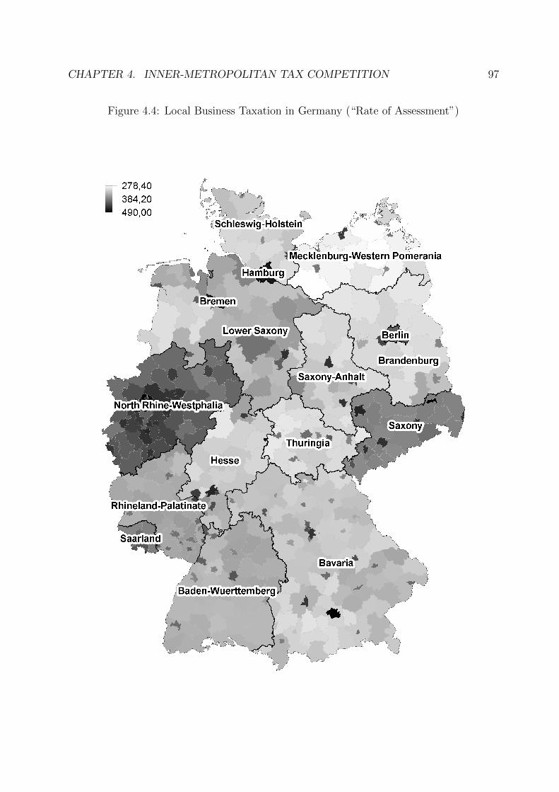
CHAPTER 4. INNER-METROPOLITAN TAX COMPETITION 97
Figure 4.4: Local Business Taxation in Germany (“Rate of Assessment”)

CHAPTER 4. INNER-METROPOLITAN TAX COMPETITION 98
situated.21
Tables 4.7 through 4.11 (see appendix) provide descriptive statistics on the most relevant
figures. Furthermore, Tables 4.12 through 4.15 show the correlation coefficients of the
four main independent variables for both approaches in their different settings. As can
be seen when looking at the coefficients for the number of surrounding municipalities and
the share of the core city, there is only a small correlation between both approaches. This
indicates that they actually cover different areas, and hence, similarities of the empirical
results can hardly be attributed to similar definitions of agglomerations. Looking at the
coefficients of the two other main independent variables indicates higher correlations. All
variables, however, concern figures that can be similar even if the municipalities covered
by an agglomeration are considerably different. Thus, we can consider the two approaches
as robustness checks for one another.
4.5 Empirical Results
Having discussed the empirical strategy, we go on with considering the results of the first
approach, which defines regions by drawing circles of some radius around core cities. For
each radius (15, 25, and 50 km) five specifications are shown.
In Table 4.2, regions with a radius of 15 km are considered.22 As the first column shows,
21We also tried some other variables, that, however, have failed to contribute to the explanation of thecore’s tax rate. Among them were the per-capita expenditures for recipients of “Unemployment Benefit II(SGB II)” to try to capture the “expenditure needs” of a municipality, and the number of passengers ofairports within an agglomeration as a possibility of taxing location-specific rents away. Moreover, includingthe quadratic form of the population of the region does not affect the results. In contrast, controlling forthe per-capita level of the core city’s debt shows a (positive) significant effect; without, however, affectingthe variables of interest.
22The effects of single basic variables on the coefficient of determination can be seen in Table 4.16 in theappendix for the case of regions of 50 km.
CHAPTER 4. INNER-METROPOLITAN TAX COMPETITION 99
there is a highly significant impact of the population share of the core in the region. If the
share of the core city increases from 0 to 100 %, the rate of assessment in the core will
increase by 34 points. The third column shows that the average size of the surrounding
municipalities is also an important determinant. If the average size increases by 1 %,
the rate of assessment increases by 12 points. This results from the declining number
of competitors due to the larger size of the surrounding municipalities. The effect of an
increase in the share of the core now becomes even more important. Going from one
extreme to the other makes the level of taxation 57 points higher. When we look directly
at the number of municipalities instead of the size, the results are confirmed. An increase
in the number of municipalities and hence the number of competitors of 1 % results in a
rate of assessment that is about 11 points lower (see columns (4) and (5)). The impact
of the share of the core city proves important again, though with a somewhat smaller
magnitude. In all specifications the population of the region as a baseline control variable
proves very important. An increase in the population of 1 % coincides with a rate of
assessment that is 15 to 26 points higher. The impact of the distance of the core city
to the next county-independent city only proves important in specifications without the
share of the core city.23 Here, the next city to be 1 km farther away results in a rate of
assessment that is roughly a quarter of a percentage point higher.
When we turn to regions of 25 km in Table 4.3, the effect of the share of the core city
becomes more important. Now, an increase in the population share of the core from 0 to
100 % results in a rate of assessment that is 63 points higher. This higher magnitude is
confirmed also in the other specifications (see columns (3) and (5)), and suggests that a
large share in a widely defined region is associated with a stronger position of the core
than a large share in a narrowly defined region. The effects of the size or number of
surrounding municipalities still prove statistically significant in most cases. They are,
23This may be due to collinearity, since the next city to be sufficiently far away implies there to be noother city in the agglomeration, and hence a large share of the core.

CHAPTER 4. INNER-METROPOLITAN TAX COMPETITION 100
Table 4.2: Local Business Taxation in Metropolitan Areas of 15 km
(1) (2) (3) (4) (5)
Constant 237 ??? 253 ??? 273 ??? 291 ??? 274 ???
(25.0) (31.2) (30.7) (32.6) (32.8)log(Pop. per Surround. Mun.) .248 12.4 ?
(5.11) (6.31)log(No. of Surround. Munic.) -11.4 ? -10.5 ?
(6.27) (6.16)Pop. Share of Core City 33.9 ?? 56.9 ??? 32.3 ??
(14.6) (18.5) (14.5)log(Pop. Region) 25.7 ??? 25.5 ??? 14.7 ?? 26.4 ??? 26.3 ???
(3.46) (5.72) (6.51) (3.52) (3.45)Distance to next City .134 .279 ? .102 .243 ? .109
(.150) (.143) (.149) (.139) (.149)
R2 0.719 0.703 0.729 0.713 0.727adj. R2 0.667 0.649 0.677 0.661 0.674Observations 118 118 118 118 118
Dependent variable: Rate of assessment of the core city of an agglomeration. Fixed-effects estima-
tion with state fixed effects. Standard errors in parentheses. A single star denotes significance at
the 10 % level, two stars at the 5 % level, and three stars at the 1 % level.
however, somewhat larger. A rise in the population per surrounding municipality of 1 %
or a decline in the number of municipalities of 1 % leads to an increase in the rate of
assessment of roughly 16 to 17 points. The impact of the population of the whole region is
as important as before, both in terms of economic and statistical significance. An increase
of the population of 1 % implies the rate of assessment in the core to be 14 to 32 points
higher. Again, the proximity of the core to the next county-independent city is important
in our specifications that exclude the share of the core city. The effect has become more
important though, with an increase in the core’s tax of 0.4 points when the next city is 1
km farther away.

CHAPTER 4. INNER-METROPOLITAN TAX COMPETITION 101
Table 4.3: Local Business Taxation in Metropolitan Areas of 25 km
(1) (2) (3) (4) (5)
Constant 210 ??? 219 ??? 272 ??? 275 ??? 272 ???
(29.7) (41.0) 40.7 43.6 (41.7)log(Pop. per Surround. Mun.) 1.50 16.7 ??
(7.12) (7.72)log(No. of Surround. Munic.) -15.9 ?? -15.7 ??
(7.96) (7.60)Pop. Share of Core City 62.5 ??? 87.1 ??? 62.1 ???
(19.6) (22.3) (19.3)log(Pop. Region) 27.2 ??? 28.4 ??? 13.5 ? 32.0 ??? 29.6 ???
(4.21) (6.93) (7.52) (4.44) (4.31)Distance to next City .187 .446 ??? .161 .412 ??? .161
(.167) (.158) (.165) (.152) (.165)
R2 0.720 0.691 0.733 0.703 0.731adj. R2 0.669 0.635 0.681 0.649 0.679Observations 118 118 118 118 118
Dependent variable: Rate of assessment of the core city of an agglomeration. Fixed-effects estima-
tion with state fixed effects. Standard errors in parentheses. A single star denotes significance at
the 10 % level, two stars at the 5 % level, and three stars at the 1 % level.
Table 4.4 shows the results for agglomerations that are defined as the municipalities within
a radius of 50 km around the city. Both the size or number of the surrounding municipalities
and the share of the core still prove important. The magnitude of the fragmentation effect
remains at the same level as before. Thus, our conjecture that this effect becomes smaller
with an increasing radius of the region cannot be confirmed.24 Compared to the preceding
definitions of regions the effect of the core city’s share in the region, however, has become
more important. The (hypothetical) difference between a city that covers the whole region
24We can see, however, that the coefficients of determination in those specifications that include onlya fragmentation variable, but not the share-of-core variable (columns (2) and (4)), become smaller, thelarger the region we consider.

CHAPTER 4. INNER-METROPOLITAN TAX COMPETITION 102
of a radius of 50 km and a city of infinitesimal size would imply a 194 to 225 points higher
rate of assessment. The impact of the population of the whole region has become smaller.
This is because the broader definition of regions covers also population from farther away.
A population that is larger by 1 % is accompanied by an increase in the rate of assessment
of 6 to 29 points. The distance to the next county-independent city proves to be somewhat
less important than before, both in terms of economic and statistical significance.
As the coefficients of determination in all definitions of regions show, the administrative
structure, population figures, and the proximity to the next county-independent city can
explain about 60 to 73 % of the variation in the level of local business taxation.
After having discussed the results for the distance-based approach, we go on with the second
approach, that defines regions in a different fashion. Rather than simply relying on radii
around core cities that are the same for each city, we now focus for two different parameters
on population densities in the space. We start with ranking surrounding municipalities
according to their distance to the core. Then, so many municipalities from this list are
added to the core until the cumulative population density of the resulting region remains
roughly constant. The definition of the region is completed when the cumulative population
density from the core to some surrounding municipality n exceeds that from the core to the
surrounding municipality n + 20 by no more than q % (with q = 1, 10).25 This approach
captures the “agglomeration mountain” that exposes itself from the flat country (see again
Figure 4.3).26
Following this idea for q = 10, we obtain the results displayed in Table 4.5. The first
25We also tried a different span (n + 10) and different values for q (2, 5). The larger the span and thesmaller q, the larger the agglomerations. The empirical results went in the anticipated directions.
26Since in few cases cities are part of a plateau of population density, a surrounding area of zero muni-cipalities can result. These observations are dropped, so that we are left with only 112 and 116 out of 118observations, respectively.

CHAPTER 4. INNER-METROPOLITAN TAX COMPETITION 103
Table 4.4: Local Business Taxation in Metropolitan Areas of 50 km
(1) (2) (3) (4) (5)
Constant 218 ??? 216 ??? 313 ??? 282 ??? 313 ???
(44.8) (65.6) (56.3) (67.0) (56.6)log(Pop. per Surround. Mun.) 1.71 19.6 ???
(8.34) (7.41)log(No. of Surround. Munic.) -15.1 ? -19.4 ???
(8.73) (7.39)Pop. Share of Core City 194 ??? 225 ??? 201 ???
(32.0) (33.3) (31.2)log(Pop. Region) 22.0 ??? 24.5 ??? 5.99 28.7 ??? 25.4 ???
(5.66) (9.27) (8.16) (6.68) (5.65)Distance to next City .030 .374 ? -.059 .318 -.059
(.173) (.192) (.172) (.192) (.172)
R2 0.714 0.609 0.733 0.620 0.733adj. R2 0.662 0.537 0.681 0.551 0.681Observations 118 118 118 118 118
Dependent variable: Rate of assessment of the core city of an agglomeration. Fixed-effects estima-
tion with state fixed effects. Standard errors in parentheses. A single star denotes significance at
the 10 % level, two stars at the 5 % level, and three stars at the 1 % level.
column shows the rate of assessment of the core city to be 85 points higher when the share
of the core increases from 0 to 100 %. This result is roughly confirmed in columns (3) and
(5), and the magnitude resembles the figures from the agglomerations of a radius of 25 km
in approach 1. Turning to columns (2) and (3) we see a rise in the size of surrounding
municipalities of 1 % to increase the core’s tax rate by 11 to 14 points. An increase in the
number of municipalities of 1 % implies a 13 to 20 points lower tax rate (see columns (4)
and (5)). Again, the magnitudes are similar to those in approach 1. Also the relevance of
the population of the region is about as high as before, with an increase of 12 to 33 points
resulting from a population increase of 1 %. If the next county-independent city is located

CHAPTER 4. INNER-METROPOLITAN TAX COMPETITION 104
Table 4.5: Local Business Taxation in Metropolitan Areas with Parameter of 10 %
(1) (2) (3) (4) (5)
Constant 214 ??? 328 ??? 224 ??? 294 ??? 227 ???
(28.0) (22.5) (27.3) (20.5) (27.6)log(Pop. per Surround. Mun.) 11.1 ?? 14.0 ???
(5.79) (5.08)log(No. of Surround. Munic.) -20.2 ??? -12.6 ??
(4.56) (4.87)Pop. Share of Core City 84.8 ??? 89.4 ??? 62.9 ???
(16.8) (16.3) (18.4)log(Pop. Region) 25.1 ??? 11.8 ??? 20.4 ??? 33.1 ??? 33.4 ???
(3.18) (3.61) (3.52) (4.70) (4.45)Distance to next City .059 .098 .204 .246 ? .202
(.133) (.157) (.139) (.148) (.140)
R2 0.720 0.658 0.742 0.706 0.739adj. R2 0.666 0.591 0.688 0.649 0.686Observations 112 112 112 112 112
Dependent variable: Rate of assessment of the core city of an agglomeration. Fixed-effects estima-
tion with state fixed effects. Standard errors in parentheses. A single star denotes significance at
the 10 % level, two stars at the 5 % level, and three stars at the 1 % level.
1 km farther away, the tax in the core will be up to a quarter of a point higher.
When we alternatively employ this second approach with a different parameter, q = 1, we
get the results in Table 4.6. This parameter ensures that the agglomerations are larger,
because now a smaller decline in the cumulative population density is required. The
importance of the core city’s share is thus a bit larger than before. An increase in the
share from 0 to 100 % goes along with an increase in the rate of assessment of 70 to 102
points (see specifications (1), (3) and (5)). The impact of the fragmentation of the region
proves to be as important as before. When the size of the surrounding municipalities

CHAPTER 4. INNER-METROPOLITAN TAX COMPETITION 105
Table 4.6: Local Business Taxation in Metropolitan Areas with Parameter of 1 %
(1) (2) (3) (4) (5)
Constant 220 ??? 347 ??? 218 ??? 294 ??? 225 ???
(28.4) (19.3) (27.1) (20.3) (27.5)log(Pop. per Surround. Mun.) 14.5 ?? 16.2 ???
(5.95) (5.11)log(No. of Surround. Munic.) -23.2 ??? -14.1 ???
(4.57) (5.03)Pop. Share of Core City 98.8 ??? 102 ??? 70.3 ???
(17.7) (17.0) (19.9)log(Pop. Region) 23.2 ??? 8.09 ??? 21.0 ??? 35.9 ??? 35.0 ???
(3.07) (2.47) (3.02) (5.44) (5.15)Distance to next City .110 .095 .276 ?? .285 ? .267 ?
(.133) (.157) (.138) (.148) (.140)
R2 0.712 0.641 0.739 0.699 0.734adj. R2 0.659 0.575 0.688 0.643 0.681Observations 116 116 116 116 116
Dependent variable: Rate of assessment of the core city of an agglomeration. Fixed-effects estima-
tion with state fixed effects. Standard errors in parentheses. A single star denotes significance at
the 10 % level, two stars at the 5 % level, and three stars at the 1 % level.
increases by 1 % or the number of municipalities declines by 1 %, the tax rate will be 14 to
23 points higher. Also the impacts of the total population of the region and the proximity
to the next city are similar to the first parameter setting. A rise in the population of the
region of 1 % implies the rate of assessment in the core to be 8 to 36 points higher. If the
next city is located 1 km farther away, a rate of assessment results that is about up to a
quarter of a point higher.
As we have seen, the results from the first approach are confirmed by the second approach
(with even higher levels of R2 of 64 to 74 %). Both variables that aim at describing the

CHAPTER 4. INNER-METROPOLITAN TAX COMPETITION 106
administrative structure within agglomerations, the number or size of the surrounding
municipalities on the one hand and the share of the core city in the agglomeration on the
other hand, have proven important throughout the majority of specifications presented in
this section.27 Hence, we can conclude that the administrative structure is an important
factor in explaining the level of local business taxation in core cities of metropolitan areas.
4.6 Conclusions
This chapter has considered the question of whether the spatial administrative structure
of municipalities affects the level of local business taxation. We examined the tax policy
of core cities of metropolitan areas, in which the design of borders can be considered to be
rather arbitrary. Due to the differences in the border design among agglomerations, the
respective core cities are facing different circumstances in deciding upon local tax policy.
On the one hand, cities could be affected by their position relative to the surrounding
area, and on the other hand they may be affected by the administrative structure of the
surrounding area itself.
Initially we considered the standard tax-competition model established by Zodrow and
Mieszkowski. Here, the two aspects just mentioned are analyzed theoretically. As a first
result, it is shown that an increasing number of surrounding municipalities (and hence
competitors) lowers the level of taxation in the core city. The second result states that
having a larger share in the agglomeration goes along with a higher tax rate of the core
city.
27When the analysis is restricted to the old West German states the effect of the share shows to bestronger, while the effect of the surrounding area is somewhat weaker. The opposite holds when only thenewly formed German states are considered.

CHAPTER 4. INNER-METROPOLITAN TAX COMPETITION 107
Before empirical analysis can be applied, one has to think about how to define agglo-
merations. Since different concepts appear to be reasonable, we establish two approaches
that try to represent different ideas. The first approach simply considers all municipalities
that are located within a certain distance to the core city to be part of an agglomeration.
The second approach is more subtle. It sorts surrounding municipalities according to their
distance to the core, and adds them to the agglomeration until the cumulative population
density from the core to the respective municipality is approaching a constant value. This
allows the area of an agglomeration to differ from city to city.
Based on these two approaches, each of them performed with different parameters, we apply
German data and in doing so focus on county-independent cities as cores of agglomerations.
To capture differences in the administrative structure we rely basically on two kinds of
indicators. The position of the core relative to the surrounding area is measured by the
core’s population share in the agglomeration. The design of borders in the surrounding
area is described by focusing on two numbers. Both the number of municipalities and their
average size are used to describe the degree of fragmentation.
It is shown that the theoretical predictions can be confirmed empirically. In metropolitan
areas a rise in the number of surrounding municipalities lowers the level of taxation in the
core. The result is confirmed when we use the average size of surrounding municipalities
instead. Since smaller surrounding municipalities imply a larger number of competitors,
the level of taxation will decrease. Furthermore, the relative position of the core in the
agglomeration proves important. The larger the share of the core in its agglomeration the
higher its tax rate. Hence, not only the competitors prove important, but also the position
of the core city itself. The effect of the share of the core city becomes more important
when the region that is considered becomes larger, since a given share in a large region is
associated with a more powerful position of this city than the same share in a small region.
All these results hold true for both concepts of defining agglomerations, for the distance-

CHAPTER 4. INNER-METROPOLITAN TAX COMPETITION 108
based as well as for the density-based approach. They explain up to three quarters of the
variation in local business taxation. This leads to the conclusion that the administrative
structure of a metropolitan area is a crucial determinant of tax policy in the core. We
can expect that both consolidations of municipalities including the core and those just
affecting the surrounding area can strengthen the core in its power to charge taxes. This
includes a reduction in the level of that part of tax competition that results from positive
externalities of core cities.
It is left for future research to look into the surrounding areas of core cities to trace
the determinants of tax policy in the suburbs. Furthermore, whether reverse impacts
exist could be analyzed: One could raise the question of whether the level of business
taxation exerts effects on the administrative structure. Also, the reaction of firms could
be considered. On the one hand, where firms locate within an agglomeration as a reaction
to different designs of borders is a subject of interest. On the other hand, the question
remains as to the benefits to a region which redesigns its borders (in terms of attractions
of firms), and hence further interregional issues could be analyzed.

CHAPTER 4. INNER-METROPOLITAN TAX COMPETITION 109
Appendix
Table 4.7: Descriptive Statistics (Regions of 15 km)
Variable Obs. Mean Standard Dev. Min Max
Tax Rate Core 118 415 37.2 300 490Pop. Core 118 229382 383510 34719 3416255Pop. Region 118 533841 560748 72125 3439531Pop. Share of Core City 118 .466 .214 .056 .993Pop. per Surr. Munic. 118 27993 51894 954 267950No. of Surr. Munic. 118 22.0 15.3 2 80Distance to next City 118 30.4 18.1 2.36 89.9
Tax Rate Core: “rate of assessment”. Region comprises core and surrounding municipalities. Distance in
kilometers.

CHAPTER 4. INNER-METROPOLITAN TAX COMPETITION 110
Table 4.8: Descriptive Statistics (Regions of 25 km)
Variable Obs. Mean Standard Dev. Min Max
Tax Rate Core 118 415 37.2 300 490Pop. Core 118 229382 383510 34719 3416255Pop. Region 118 1006343 987922 129565 4053493Pop. Share of Core City 118 .266 .171 .032 .889Pop. per Surr. Munic. 118 22508 36806 890 160605No. of Surr. Munic. 118 64.2 41.5 11 247Distance to next City 118 30.4 18.1 2.36 89.9
Tax Rate Core: “rate of assessment”. Region comprises core and surrounding municipalities. Distance in
kilometers.
Table 4.9: Descriptive Statistics (Regions of 50 km)
Variable Obs. Mean Standard Dev. Min Max
Tax Rate Core 118 415 37.2 300 490Pop. Core 118 229382 383510 34719 3416255Pop. Region 118 2815419 2533411 304597 10038362Pop. Share of Core City 118 .102 .107 .012 .747Pop. per Surr. Munic. 118 17934 26361 1366 89780No. of Surr. Munic. 118 254 154 48 911Distance to next City 118 30.4 18.1 2.36 89.9
Tax Rate Core: “rate of assessment”. Region comprises core and surrounding municipalities. Distance in
kilometers.

CHAPTER 4. INNER-METROPOLITAN TAX COMPETITION 111
Table 4.10: Descriptive Statistics (Regions 10 %)
Variable Obs. Mean Standard Dev. Min Max
Tax Rate Core 112 415 37.5 300 490Pop. Core 112 236045 392392 34719 3416255Pop. Region 112 794969 1120851 43506 5866000Pop. Share of Core City 112 .410 .189 .029 .887Pop. per Surr. Munic. 112 18357 32004 632 146789No. of Surr. Munic. 112 43.4 31.5 1 151Distance to next City 112 31.4 18.0 2.36 89.9
Tax Rate Core: “rate of assessment”. Region comprises core and surrounding municipalities. Distance in
kilometers.
Table 4.11: Descriptive Statistics (Regions 1 %)
Variable Obs. Mean Standard Dev. Min Max
Tax Rate Core 116 415 37.3 300 490Pop. Core 116 231949 386298 34719 3416255Pop. Region 116 1435340 2569809 43879 14746017Pop. Share of Core City 116 .330 .202 .017 .911Pop. per Surr. Munic. 116 14196 22581 728 132404No. of Surr. Munic. 116 102 106 1 520Distance to next City 116 30.8 18.0 2.36 89.9
Tax Rate Core: “rate of assessment”. Region comprises core and surrounding municipalities. Distance in
kilometers.

CHAPTER 4. INNER-METROPOLITAN TAX COMPETITION 112
Table 4.12: Correlation of the Number of Surrounding Municipalities
Variable Reg. 15 km Reg. 25 km Reg. 50 km Reg. 10 % Reg. 1 %
Regions of 15 km 1.000Regions of 25 km 0.911 1.000Regions of 50 km 0.786 0.925 1.000Regions 10 % 0.185 0.216 0.144 1.000Regions 1 % 0.037 0.192 0.228 0.583 1.000
Table 4.13: Correlation of the Population per Surrounding Municipality
Variable Reg. 15 km Reg. 25 km Reg. 50 km Reg. 10 % Reg. 1 %
Regions of 15 km 1.000Regions of 25 km 0.942 1.000Regions of 50 km 0.815 0.935 1.000Regions 10 % 0.952 0.966 0.891 1.000Regions 1 % 0.926 0.938 0.917 0.932 1.000
Table 4.14: Correlation of the Population Share of the Core City
Variable Reg. 15 km Reg. 25 km Reg. 50 km Reg. 10 % Reg. 1 %
Regions of 15 km 1.000Regions of 25 km 0.899 1.000Regions of 50 km 0.718 0.864 1.000Regions 10 % 0.508 0.370 0.286 1.000Regions 1 % 0.524 0.364 0.244 0.853 1.000

CHAPTER 4. INNER-METROPOLITAN TAX COMPETITION 113
Table 4.15: Correlation of the Population of the Region
Variable Reg. 15 km Reg. 25 km Reg. 50 km Reg. 10 % Reg. 1 %
Regions of 15 km 1.000Regions of 25 km 0.910 1.000Regions of 50 km 0.726 0.900 1.000Regions 10 % 0.871 0.844 0.653 1.000Regions 1 % 0.764 0.800 0.664 0.861 1.000
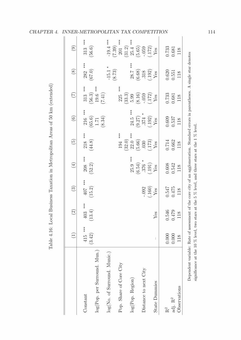
CHAPTER 4. INNER-METROPOLITAN TAX COMPETITION 114
Tab
le4.
16:
Loca
lB
usi
nes
sT
axat
ion
inM
etro
pol
itan
Are
asof
50km
(exte
nded
)
(1)
(2)
(3)
(4)
(5)
(6)
(7)
(8)
(9)
Con
stan
t41
5???
403
???
407
???
208
???
218
???
216
???
313
???
282
???
313
???
(3.4
2)(1
3.4)
(15.
2)(5
2.2)
(44.
8)(6
5.6)
(56.
3)(6
7.0)
(56.
6)lo
g(P
op.
per
Surr
ound.
Mun.)
1.71
19.6
???
(8.3
4)(7
.41)
log(
No.
ofSurr
ound.
Munic
.)-1
5.1?
-19.
4???
(8.7
3)(7
.39)
Pop
.Shar
eof
Cor
eC
ity
194
???
225
???
201
???
(32.
0)(3
3.3)
(31.
2)lo
g(P
op.
Reg
ion)
25.9
???
22.0
???
24.5
???
5.99
28.7
???
25.4
???
(6.5
4)(5
.66)
(9.2
7)(8
.16)
(6.6
8)(5
.65)
Dis
tance
tonex
tC
ity
-.09
2.3
76?
.030
.374
?-.
059
.318
-.05
9(.
160)
(.19
1)(.
173)
(.19
2)(.
172)
(.19
2)(.
172)
Sta
teD
um
mie
s–
Yes
Yes
Yes
Yes
Yes
Yes
Yes
Yes
R2
0.00
00.
546
0.54
70.
608
0.71
40.
609
0.73
30.
620
0.73
3ad
j.R
20.
000
0.47
90.
475
0.54
20.
662
0.53
70.
681
0.55
10.
681
Obse
rvat
ions
118
118
118
118
118
118
118
118
118
Dep
end
ent
vari
able
:R
ate
ofas
sess
men
tof
the
core
city
of
an
agglo
mer
ati
on
.S
tan
dard
erro
rsin
pare
nth
eses
.A
sin
gle
star
den
ote
s
sign
ifica
nce
atth
e10
%le
vel,
two
star
sat
the
5%
leve
l,an
dth
ree
stars
at
the
1%
leve
l.
CHAPTER 4. INNER-METROPOLITAN TAX COMPETITION 115
References
Baldwin, R. E. and P. Krugman (2004): Agglomeration, Integration and Tax Harmoni-
sation, European Economic Review, 48 (1), 1–23.
Boustedt, O. (1953): Die Stadtregion. Ein Beitrag zur Abgrenzung stadtischer Agglo-
merationen, Allgemeines Statistisches Archiv, 37, 13–26.
Brecht, A. (1932): Internationaler Vergleich der offentlichen Ausgaben, Grundfragen der
internationalen Politik, Heft 2, Leipzig.
Bucovetsky, S. and M. Smart (2006): The Efficiency Consequences of Local Revenue
Equalization: Tax Competition and Tax Distortions, Journal of Public Economic
Theory, 8, 119–144.
Buettner, T. (2006): The Incentive Effect of Fiscal Equalization Transfers on Tax Policy,
Journal of Public Economics, 90, 477–497.
Buettner, T. and B. Kauder (2010): Wettbewerbsposition der Stadt Frankfurt im Verhalt-
nis zum Umland, ifo Forschungsberichte, 48, Munchen.
Hatfield, J. W. and K. Kosec (2009): Federal Competition and Economic Growth, Rock
Center for Corporate Governance at Stanford University Working Paper, No. 63.
Helliwell, J. F. (1997): National Borders, Trade and Migration, Pacific Economic Review,
3, 165–185.
Hoxby, C. M. (2000): Does Competition among Public Schools Benefit Students and
Taxpayers? American Economic Review, 90 (5), 1209–1238.
Koethenbuerger, M. (2002): Tax Competition and Fiscal Equalization, International Tax
and Public Finance, 9, 391–408.

CHAPTER 4. INNER-METROPOLITAN TAX COMPETITION 116
Ohsawa, Y. (1999): Cross-Border Shopping and Commodity Tax Competition Among
Governments, Regional Science and Urban Economics, 29 (1), 33–51.
Popitz, J. (1932): Der kunftige Finanzausgleich zwischen Reich, Landern und Gemeinden,
Gutachten, erstattet der Studiengesellschaft fur den Finanzausgleich, Berlin.
Seitz, H. (2002): Der Einfluss der Bevolkerungsdichte auf die Kosten der offentlichen
Leistungserstellung, Schriften zum offentlichen Recht, Band 899, Berlin.
Zodrow, G. R. and P. Mieszkowski (1986): Pigou, Tiebout, Property Taxation, and the
Underprovision of Local Public Goods, Journal of Urban Economics, 19, 356–370.

Chapter 5
Consolidation of Municipalities and
Impact on Population Growth – A
Propensity Score Matching Approach

CHAPTER 5. CONSOLIDATION OF MUNICIPALITIES 118
Abstract
During the 1960s and 1970s, the number of municipalities in Germany was notably reduced.
Many municipalities located on the outskirts of a city lost their independent status and
became a district of the adjacent core city. This chapter analyzes the consequences of such
a reform on the population development in these city districts. In comparing incorporated
municipalities with those that remained independent, the former are found to perform
better in terms of population growth. This effect is confirmed when differences in states’
population growth rates are taken into account, and becomes stronger for municipalities
that were incorporated later and for smaller municipalities. To avoid selection bias by pos-
sibly comparing two groups with different properties, a propensity score matching approach
is employed. This allows us to compare incorporated with still independent communities
that had a similar propensity to be incorporated and, hence, similar characteristics. We
find that the propensity score is basically driven by the distance of the community to the
core city, the size in terms of population and area, and the state to which it belongs.
5.1 Introduction
The spatial structure of administrative units is an ongoing political issue. Although con-
solidations or divisions at the state or even country level are rare, local-level reforms are
a common occurrence. These reforms, which typically reduce the number of municipali-
ties, are often controversial in those municipalities that are going to lose their independent
status by being merged into a larger municipality. Since identification with one’s home
town is often very strong, broad resistance is not unexpected. However, changing settle-
ment patterns in the course of (sub-)urbanization and changing demands for public services
necessitate adjustments of administrative structures.1
1As in Chapter 4, we use the short version administrative structure instead of spatial administrativestructure.

CHAPTER 5. CONSOLIDATION OF MUNICIPALITIES 119
The literature discusses several aspects of designing and/or reforming administrative struc-
tures, at both the regional and country level. Alesina et al. (1995) provide an overview of
articles that focus on the normative perspective. Among the core arguments in favor of
larger jurisdictions are economies of scale in the production of public goods and services,
the internalization of externalities, and possible insurance against revenue shocks. Argu-
ments in opposition highlight the advantages of decentralization as including an increase
in political influence for each citizen and the possibility of serving different tastes in the
provision of public goods.2
Another strand of literature is concerned with the positive perspective, and analyzes the
determinants of (voluntary) mergers or secessions at the municipality level. Brink (2004)
provides evidence that within-municipality imbalances of wealth are relevant in the oc-
currence of split-ups in Sweden. Sørensen (2006) looks at consolidations and lists several
hindering factors. These include that the common grant for merged municipalities might
be lower than the sum of individual grants to unmerged communities; that high-revenue
municipalities will have to share their revenues when consolidated with a poorer neighbor;
and that the composition of political preferences may affect the policies implemented. By
employing Norwegian data, he finds consolidations to be more likely when efficiency gains
are expected to be large and differences in revenues and political preferences are small. Filer
and Kenny (1980) find evidence that the income distribution between city and county ex-
plains approval in consolidation referenda in the United States, but that the relevance of
economies of scale cannot be confirmed. Austin (1999) also considers incorporations in
the United States, some of which could have realized on the city’s own right. He finds
“unfavorable” migration between city and surrounding area to be an important factor in
explaining incorporations because by expanding city boundaries, the composition of voters
can be manipulated to politicians’ advantage. Exploiting tax bases by incorporation, on
2Theoretical analyses focusing on the trade-off between efficiency and heterogeneous populations orpolitical influence are provided by Alesina and Spolaore (1997) and Bolton and Roland (1997).

CHAPTER 5. CONSOLIDATION OF MUNICIPALITIES 120
the contrary, shows not to be relevant.
The consequences of incorporation are also examined in the literature. Blume (2009)
analyzes the effects of the German reforms implemented in the 1960s and 1970s on the
performance of both regions and cities. He finds that counties with an incorporated core
have less debt than regions with an independent core city. This is explained as due to
politico-economic incentives: municipalities’ politicians force counties to use efficiency gains
from the incorporation of the core city to reduce debt, with the consequence that transfers
paid by municipalities to the county can be lowered. Furthermore, cities are shown to
grow faster (in terms of gross value added) the higher their intensity of incorporation.
The explanation here focuses on politicians’ interest in being reelected. Since voters are
assumed to appreciate public expenditures more than they do debt reduction, efficiency
gains from consolidations are used for further public investment, which results in higher
growth rates.
These German reforms of the 1960s and 1970s are also the basis of this chapter. However,
instead of looking at the effects of consolidation on the core city that is expanded the
focus here is on the municipalities that were incorporated. Specifically, the interest is
in changes in population as a measure of the increased or decreased attractiveness of a
community. A community can be more or less attractive to citizens for several reasons,
some of which involve, as mentioned above, differences in wealth or political influence. The
big reforms that reduced the number of municipalities in Germany from roughly 24,000
to 8,500 occurred between 1967 and 1978. Hence, a sufficiently long time has passed to
evaluate the effects on a rather persistent factor like the population. Municipalities that
remained independent are compared with those that became a city district. Population
statistics from the pre-reform period of the early 1960s are employed, as well as current
population numbers at the municipality and city-district level.

CHAPTER 5. CONSOLIDATION OF MUNICIPALITIES 121
We employ a propensity score matching approach that links incorporated to still indepen-
dent municipalities on the basis of similar probabilities of incorporation. It is found that
these probabilities are basically driven by location, population, area, and state affiliation.
Subsequently, the estimated effect of incorporation is calculated and shows that munici-
palities that became a city district have grown faster in terms of population. This effect is
stronger for later incorporated and for small municipalities.
The chapter is organized as follows. Section 5.2 discusses the reforms and the current
situation in Germany. Section 5.3 develops the empirical strategy and provides information
on the data. Section 5.4 contains the results; Section 5.5 concludes.
5.2 Institutional Background
The number of municipalities in Germany is constantly changing or, to be more precise,
constantly declining. In 1900, Germany had approximately 77,000 municipalities; by 2008,
there were only 12,000. Of course, the loss of territory associated with the world wars
explains a significant part of the decline. However, even within the country’s current
territory, the number of municipalities in 1900 was about 45,000, remarkably more than
exist today. In the mid-1960s, the number (in West Germany) was around 24,000, with
about 95 % of the municipalities having less than 5,000 inhabitants.
Between 1967 and 1978, large reforms in the administrative structure of municipalities
were implemented, in the course of which the number of municipalities was reduced to
8,500.3 Initially, even more reductions were planned; however, in some cases municipalities
successfully resisted merger, both before and after it occurred.
3The current number of about 12,000 municipalities is explained solely by the 1990 reunification ofGermany.

CHAPTER 5. CONSOLIDATION OF MUNICIPALITIES 122
Table 5.1: Reforms of the Administrative Structure
No. Municipal. No. Municipal. Reduction No. Munic.State Before Reforms After Reforms in % in 2008
Saarland 347 50 85.59 52Hesse 2684 427 84.09 426North Rhine-Westphalia 2277 396 82.61 396Lower Saxony 4231 1029 75.68 1024Bavaria 7077 2048 71.06 2056Baden-Wurttemberg 3379 1111 67.12 1102Rhineland-Palatinate 2905 2303 20.72 2306Schleswig-Holstein 1378 1132 17.85 1119Berlin 1 1 0.00 1Hamburg 1 1 0.00 1Bremen 2 2 0.00 2
Total 24282 8500 64.99 8485
Number of municipalities before and after the reforms according to the German Federal Statistical
Office, quoted according to Puttner (1983).
According to Wagener (1969), the aims of the reforms can be grouped into five cate-
gories: promoting equal conditions of life in both urban and rural areas, strengthening
the efficiency of municipalities in rural areas, ensuring a well-arranged development and
function of urban areas, restructuring areas with respect to aspects of spatial planning
and infrastructure, and improving general-interest services. Accordingly, the reforms were
characterized by a change from historically established units to ones focused on efficient
public structures.
The mergers were realized both by voluntary agreements of municipalities and via en-
forcement. In the state of Baden-Wurttemberg, for instance, the number of municipalities
was reduced from 3,379 to 1,111, with the smallest municipalities inhabited by at least

CHAPTER 5. CONSOLIDATION OF MUNICIPALITIES 123
8,000 people. Municipalities that merged voluntarily were granted funds. The reforms in
Bavaria were of similar intensity and reduced the number of municipalities in that state
from 7,077 to 2,048. As can be seen in Table 5.1, the reforms in Saarland, Hesse, North
Rhine-Westphalia, and Lower Saxony were even more intense. In all these states, the num-
ber of municipalities declined by more than 75 %. The intensity of the reforms was lower
in Rhineland-Palatinate and Schleswig-Holstein, with reductions of only about 20 %. In
the federal city states of Berlin, Hamburg, and Bremen, no changes have been realized.
After these reforms, there have been just a few further adjustments, as the last column
shows. The number of municipalities has remained almost constant over the past 30 years.
5.3 Identification Strategy and Data
The aim of this chapter is to discover whether the incorporation of a municipality into
a core city is a causal factor in either faster or slower growth in the incorporated unit
in terms of population. For this purpose, municipalities that were consolidated with a
core city are compared with ones that remained independent. This is done by estimating
the counterfactual outcome, which tells how fast an incorporated municipality would have
grown if it had not been incorporated (or vice versa). Comparing these counterfactuals
with the actual growth rates gives the effect of incorporation.
The sample includes all cities that were county-independent in 1961 and remained so until
2008 (“Kreisfreie Stadte”), restricted to the territory of former West Germany. Two groups
of (surrounding) communities of these core cities are looked at. The first group comprises
municipalities that were incorporated into a city in the course of the reforms (the treatment
group). For these, the population figures from when they were still independent in 1961
are compared with their population as a city district in 2008. Since appropriate data are

CHAPTER 5. CONSOLIDATION OF MUNICIPALITIES 124
not available for all cities, particularly when a city district is not identical to the former
municipality, this group contains 124 observations. The second group comprises those
municipalities in the surrounding area of a core city that have remained independent until
the present day (the control group). The surrounding area is restricted to a circle of 12.5
km around the center of the core city.4 Furthermore, only those (in 1961 and 2008 county-
dependent) surrounding municipalities are considered that have for their part experienced
no mergers or break-ups. Based on these restrictions, 447 observations remain.
To compare the treatment and the control group without further adjustments is not a valid
identification strategy. Employing standard OLS techniques would likely entail a selection
bias. The municipalities that lost their independent status were certainly not selected
randomly; rather, certain characteristics are likely to have influenced the probability of
being incorporated. However, when, for instance, small surrounding municipalities were
more likely to be incorporated, higher population growth might have occurred not because
of the incorporation itself, but because of an increased preference of potential citizens for
smaller communities. The same argument holds for other factors, like the distance from
the community to the center of the core city.
Since such factors notably affect the probability of being merged with the respective core
city, the likely occurrence of a selection bias has to be bypassed. A strategy has to be
developed that allows comparing treated and untreated municipalities that have similar
(pre-treatment) characteristics. Optimally, municipalities should differ only with respect
to whether or not they have been treated, all other characteristics being equal. Since it
is hardly possible to match on every covariate, however, such characteristics should be
condensed into one number. This is done by the propensity score matching approach
suggested by Rosenbaum and Rubin (1983). According to this approach, a probability of
incorporation is calculated in a first step. In doing so, factors likely to affect the probability
4This distance equals the longest distance of an incorporated municipality in the data set.

CHAPTER 5. CONSOLIDATION OF MUNICIPALITIES 125
are used in a probit regression as covariates X, with a binary variable (treated: T = 1,
untreated: T = 0) as the dependent variable:5
Prob(T = 1|X) = φ(X ′β).
After having found such propensity scores for both members of the treatment group and
the control group, and if the scores of both groups overlap (common support), actual
matching of appropriate partners is possible. This procedure is intended to make the
groups comparable by possibly omitting such observations that are causing the groups
to be different. Four different versions of propensity score matching are employed in the
following.
One-to-one matching is the simplest way to match treated with untreated observations.
In this version, every treated municipality is matched with the untreated neighbor (in the
probability space) that has the closest propensity score. Several treated municipalities can
be matched with the same untreated one (with replacement). To avoid imprecise matches,
a caliper is introduced. This restricts matches to those having a sufficiently small difference
in propensity scores between treated and untreated case.
In a more general approach, one can match each treated case with an unweighted average
of k nearest neighbors, which is called k-nearest-neighbors matching. We run this method
with 10 neighbors. Since a caliper is also used here, matching will be conducted with less
than 10 neighbors when there is not a sufficient number of neighbors available within the
caliper. A higher number of neighbors to compare with provides the advantage of exploiting
more information and being less subject to outliers (smaller variance). However, this is at
the expense of a less precise matching (larger bias). The one-to-one matching is a special
case of k-nearest-neighbors matching; that is, it uses only one neighbor.
5Alternatively, a logit model could be used.

CHAPTER 5. CONSOLIDATION OF MUNICIPALITIES 126
A different approach based on a similar idea is radius matching. Here, the treated observa-
tion is matched to an unweighted average of those untreated observations with a propensity
score within a certain radius, e.g., all untreated cases that have a propensity score up to 1.5
percentage points higher or lower than the treated case. This is not the same as k-nearest-
neighbors matching with a caliper. Radius matching captures all neighbors within a certain
radius, no matter how many there are. K-nearest-neighbors matching with a caliper, in
contrast, captures a certain number of neighbors, no matter how many there are available
within the caliper. Only if k is greater than the number of observations within the caliper,
and hence all neighbors within the caliper are captured, radius and k-nearest-neighbors
matching can produce identical matches (given radius = caliper).
As a fourth and final method, kernel matching is considered. This method resembles
radius matching, but it compares the treated case with a weighted average of untreated
cases given a certain bandwidth. The weights depend on the difference in propensity score.
The farther away the matching partner in terms of propensity scores, the smaller the
weight it is given. Accordingly, this approach puts more weight on near neighbors than
on those farther away in the probability space. When kernel matching is employed with a
uniform kernel function, it is the same as radius matching. However, we use the common
epanechnikov kernel with decreasing weights.
In all matching approaches, calipers – or a bandwidth in the case of kernel matching –
of 1.5 % are used. This means that the propensities of the treated and the matched
untreated case(s) are not allowed to differ by more than 1.5 percentage points, which is
intended to avoid imprecise matches. This is done at the expense of a smaller number of
observations exploited (larger variance), but does ensure against comparing treated and
untreated municipalities that are too different from one another in terms of propensity
score (smaller bias). Accordingly, setting up calipers circumvents the investigation of the

CHAPTER 5. CONSOLIDATION OF MUNICIPALITIES 127
overlap and common support issue.6
Given the matching of observations and the resulting appraisals for counterfactual out-
comes, the average treatment effect on the treated (ATT) can be calculated:7
ATT =1
n
(n∑i=1
Pop 2008i − Pop 1961iPop 1961i
−m∑j=1
αjPop 2008j − Pop 1961j
Pop 1961j
).
This entails nothing more than calculating the extent to which population growth of com-
parable incorporated (i) and still independent municipalities (j) differs. The significance
of this treatment effect can be tested with the usual t-statistics.
Finally, to ensure the validity of the results, it must be proven that the treatment and the
control group have become sufficiently similar. Gadd et al. (2008), for instance, ensure that
this “balancing property” holds by looking at every variable used to explain the propensity
score. Only if it is certain that the differences between the average value of each variable in
the treatment and the control group are insignificant, can it be concluded that the groups
are comparable.8
The data set contains information on the population from both the pre-reform period and
latest figures available currently. The first is taken from the population census 1961; the
6Without calipers, one would have to use another method of ensuring that only those observations inthe control group that are similar to the treated observations are used.
7The number of (exploited) observations in the treatment group is denoted n, the number of (exploited)observations in the control group is denoted m, and αj indicates the different weights for the untreatedobservations that can follow from all matching methods.
8Another issue regarding the validity of the results concerns unconfoundedness. According to this andwith T as treatment, Y0 and Y1 as potential outcomes, X as pre-treatment characteristics, and p(X) aspropensity score, assignment to the treatment has to fulfill T ⊥ Y0, Y1|X, which can be shown to implyT ⊥ Y0, Y1|p(X). This requires that “systematic differences in outcomes between treated and comparisonindividuals [municipalities] with the same values for covariates are attributable to treatment” (Caliendoand Kopeinig (2008)). However, since unconfoundedness cannot be tested directly, we only assume thecondition to hold. For further details, see Rosenbaum and Rubin (1983).

CHAPTER 5. CONSOLIDATION OF MUNICIPALITIES 128
recent data are derived from the local statistics of the German Federal Statistical Office
from 2008 and from publications of the respective cities from about the same time.
The variables used are basically needed to explain the incorporation probabilities of muni-
cipalities. Since these are driven by conditions prevailing in the period prior to the reforms,
only variables from the pre-reform period or time-invariant variables come into play.9 As
to covariates that might be relevant, location of the respective municipality is an obvious
choice. It is reasonable to assume that the farther away from the center of a core city a
municipality is located, the more likely it is to remain independent. Using the geographic
coordinates of each municipality in both the treatment and the control group provides the
distance of each municipality to the center of the respective core city.10
Another potentially important factor is the size of the surrounding municipality, both in
terms of population and area. It is reasonable to expect that a surrounding municipality
is more likely to lose its independent status the smaller it is. Also the size of the core city
might matter. Large cities could incorporate more or less intensively than smaller ones.
For this reason, the population and the area of the core city are included as well.
Numerous other statistics are available at the county level only. However, attributing
the county figure to a municipality can provide some relevant information. For example,
the 1966 per-capita debt level for both the core city and the (county of the) surrounding
municipality is of interest, since the public finances situation should influence whether
a municipality can remain independent.11 Furthermore, political variables are included.
9In a narrow sense, variables not only must originate in the pre-reform period, but also must beunaffected by a possible anticipation of the reforms.
10In the case of overlapping surrounding areas, a non-incorporated municipality is related to the nearestcore city. Official central points are used as coordinates of core cities, while the coordinates of surroundingmunicipalities are based on centroid considerations.
11Debt at the county level comprises both the debt of the county itself and of the respective munici-palities.
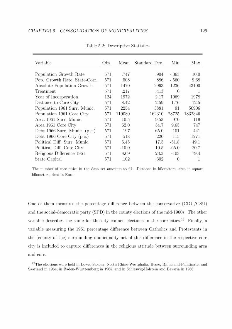
CHAPTER 5. CONSOLIDATION OF MUNICIPALITIES 129
Table 5.2: Descriptive Statistics
Variable Obs. Mean Standard Dev. Min Max
Population Growth Rate 571 .747 .904 -.363 10.0Pop. Growth Rate, State-Corr. 571 .508 .886 -.560 9.68Absolute Population Growth 571 1470 2963 -1236 43100Treatment 571 .217 .413 0 1Year of Incorporation 124 1972 2.17 1969 1978Distance to Core City 571 8.42 2.59 1.76 12.5Population 1961 Surr. Munic. 571 2254 3881 91 50906Population 1961 Core City 571 119080 162310 28725 1832346Area 1961 Surr. Munic. 571 10.5 9.53 .970 119Area 1961 Core City 571 62.0 54.7 9.65 747Debt 1966 Surr. Munic. (p.c.) 571 197 65.0 101 441Debt 1966 Core City (p.c.) 571 518 220 115 1271Political Diff. Surr. Munic. 571 5.45 17.5 -51.8 49.1Political Diff. Core City 571 -10.0 10.5 -65.0 20.7Religious Difference 1961 571 8.69 23.3 -103 79.4State Capital 571 .102 .302 0 1
The number of core cities in the data set amounts to 67. Distance in kilometers, area in square
kilometers, debt in Euro.
One of them measures the percentage difference between the conservative (CDU/CSU)
and the social-democratic party (SPD) in the county elections of the mid-1960s. The other
variable describes the same for the city council elections in the core cities.12 Finally, a
variable measuring the 1961 percentage difference between Catholics and Protestants in
the (county of the) surrounding municipality net of this difference in the respective core
city is included to capture differences in the religious attitude between surrounding area
and core.
12The elections were held in Lower Saxony, North Rhine-Westphalia, Hesse, Rhineland-Palatinate, andSaarland in 1964, in Baden-Wurttemberg in 1965, and in Schleswig-Holstein and Bavaria in 1966.

CHAPTER 5. CONSOLIDATION OF MUNICIPALITIES 130
The state the municipality belongs to may also have an impact on the probability of a
merger. Since some states have reduced the number of municipalities to a greater extent
than have others (see Section 5.2), state dummies are added as additional explanatory
variables. Moreover, a dummy variable indicating whether the respective core city is a
state capital is included.
Descriptive statistics on all relevant variables are provided in Table 5.2.
5.4 Empirical Results
As set out above the identification strategy involves four steps: (1) explaining the proba-
bility of incorporation, (2) matching observations, (3) calculating the treatment effect, and
(4) ensuring validity by checking the balancing property.
We start by running a probit model to explain the probability of incorporation (propensity
score). This yields the results shown in the left part of Table 5.3.13 As the table reveals, the
distance of the municipality from the center of the core city is the most significant factor
in creating the propensity score. The farther from the core city’s center a municipality is,
the less likely it is to be incorporated. The size of the municipality is important also. The
bigger the municipality’s population, the less likely it is to be incorporated. The opposite
holds for an increase in area, however. A larger area is associated with a significantly
higher propensity score. These two effects together mean that being incorporated is more
likely the lower the population density. This is in line with the argument that incorpora-
tion is done to strengthen the efficiency of administrations, since municipalities with low
population density are hardly able to exploit economies of scale in the provision of public
13The results of an identical logit model are shown in the right part of the table for comparison. However,in the following, we restrict the analysis to the probit results.

CHAPTER 5. CONSOLIDATION OF MUNICIPALITIES 131
goods and services. The size of the core city shows opposite (and insignificant) effects. A
higher population and a smaller area increase the probability of incorporating surrounding
municipalities. This can be explained by the fact that such cities need space for further
population development.
Among the county-level variables, a higher per-capita debt level of the (county of a) sur-
rounding municipality increases its probability of incorporation. Moreover, a core city
is more likely to be enlarged when its debt level is higher. Both effects, however, are
insignificant. A conservative municipality is more likely to remain independent than a
social-democratic one. This effect, which may result from conservative communities hold-
ing more traditional attitudes, is almost significant. Furthermore, a conservative core city
will incorporate more intensively, but this effect is not significant: surrounding municipali-
ties that are considered to be richer than the core city, and consequently more conservative
politically, may be a motivation for conservative politicians to enhance their electoral base
by an act of incorporation. Concerning religiosity, a significant effect can be found that
shows incorporation is more likely the more Catholic the surrounding municipality and the
less Catholic the core city.
Looking at the state dummies provides clues as to the lower intensity of consolidations
in Schleswig-Holstein and Rhineland-Palatinate, as mentioned in Section 5.2. On the
contrary, Lower Saxony shows a higher intensity of reforms. Regarding state capitals,
an (insignificant) effect of a higher propensity of incorporations is found: when cities are
considered to be willing to be enhanced, this could result from a bias of state politicians
towards the city in which their parliament is located. All the variables contribute to a
pseudo R2 of about 45 %.14
14The results of the analysis below are very similar when all variables with z-values below 1 are excludedfrom the probit regression. For a discussion regarding the specification of propensity score models, seeCaliendo and Kopeinig (2008).
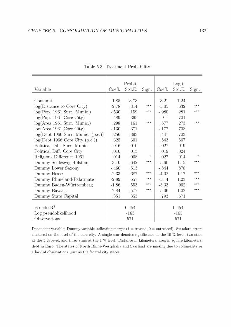
CHAPTER 5. CONSOLIDATION OF MUNICIPALITIES 132
Table 5.3: Treatment Probability
Probit LogitVariable Coeff. Std.E. Sign. Coeff. Std.E. Sign.
Constant 1.85 3.73 3.21 7.24log(Distance to Core City) -2.78 .314 ??? -5.05 .632 ???
log(Pop. 1961 Surr. Munic.) -.530 .159 ??? -.980 .281 ???
log(Pop. 1961 Core City) .489 .365 .911 .701log(Area 1961 Surr. Munic.) .298 .161 ??? .577 .273 ??
log(Area 1961 Core City) -.130 .371 -.177 .708log(Debt 1966 Surr. Munic. (p.c.)) .256 .393 .447 .703log(Debt 1966 Core City (p.c.)) .325 .301 .543 .567Political Diff. Surr. Munic. -.016 .010 -.027 .019Political Diff. Core City .010 .013 .019 .024Religious Difference 1961 .014 .008 ? .027 .014 ?
Dummy Schleswig-Holstein -3.10 .642 ??? -5.60 1.15 ???
Dummy Lower Saxony -.460 .513 -.844 .878Dummy Hesse -2.33 .687 ??? -4.02 1.17 ???
Dummy Rhineland-Palatinate -2.89 .657 ??? -5.14 1.23 ???
Dummy Baden-Wurttemberg -1.86 .553 ??? -3.33 .962 ???
Dummy Bavaria -2.84 .577 ??? -5.06 1.02 ???
Dummy State Capital .351 .353 .793 .671
Pseudo R2 0.454 0.454Log pseudolikelihood -163 -163Observations 571 571
Dependent variable: Dummy variable indicating merger (1 = treated, 0 = untreated). Standard errors
clustered on the level of the core city. A single star denotes significance at the 10 % level, two stars
at the 5 % level, and three stars at the 1 % level. Distance in kilometers, area in square kilometers,
debt in Euro. The states of North Rhine-Westphalia and Saarland are missing due to collinearity or
a lack of observations, just as the federal city states.

CHAPTER 5. CONSOLIDATION OF MUNICIPALITIES 133
After using the estimated coefficients of the probit model to predict the propensity scores,
we proceed to the matching procedure and the resulting treatment effects. The left part
of Table 5.4 shows the results for the four matching methods outlined in the preceding
section. All four methods estimate a large positive and significant effect of incorporation
on population growth. Accordingly, a municipality that became a city district grows by
about 29 percentage points more than it would have if it had not been merged with the core
city. Municipalities that remained independent grew on average by only about 77 %; those
that were incorporated grew by about 106 % (not shown in the table). The significance of
the effects is not affected when bootstrapped standard errors, which attempt to take into
account that the propensity score is estimated, are considered.15
The treatment effects just discussed are based on comparisons of incorporated and still
independent municipalities that may be located in different states. Since the population
growth rates among the states differed notably in the period considered – ranging from
-3.9 % in Saarland to +38.5 % in Baden-Wurttemberg – it would seem relevant to take
this fact into account.16 The treatment effect can be adjusted for the different state growth
rates by subtracting this difference in the calculation of the figures of every single match.
Hence, it is no longer the population growth rate of a municipality itself that is considered,
but the extent to which the population growth rate exceeds that of the state in which
the municipality is located. The results are displayed in the right part of Table 5.4. As
can be seen, the treatment effect still amounts to about 29 percentage points and is again
significant. Municipalities that have been incorporated grew 80 percentage points more
than their respective state; those that remained independent grew only about 51 percentage
points more.
15Although widely used in the literature, it is unclear whether bootstrapped standard errors are validin the context of propensity score matching (see Abadie and Imbens (2006)).
16Indeed, state differences have already been taken into account in the estimation of propensity scores,but now states’ differences in population growth, rather than in the intensity of incorporation, are con-cerned.

CHAPTER 5. CONSOLIDATION OF MUNICIPALITIES 134
Table 5.4: Average Treatment Effect on the Treated
Population Growth RateState-Corrected
Matching Method Coeff. (Std.E.) Coeff. (Std.E.)
One-to-one (Caliper: 1.5 %)Average Treatment Effect on the Treated .296 (.169) ? .292 (.167) ?
(Bootstrapped Standard Errors) (.148) ?? (.144) ??
10-Nearest-Neighbors (Caliper: 1.5 %)Average Treatment Effect on the Treated .294 (.152) ? .297 (.149) ??
(Bootstrapped Standard Errors) (.144) ?? (.143) ??
Radius (Caliper: 1.5 %)Average Treatment Effect on the Treated .282 (.153) ? .288 (.150) ?
(Bootstrapped Standard Errors) (.149) ? (.146) ??
Kernel (Epanechnikov, Bandwidth: 1.5 %)Average Treatment Effect on the Treated .291 (.155) ? .294 (.152) ?
(Bootstrapped Standard Errors) (.159) ? (.157) ?
Number of observations: 133 to 524 (treated: 80, untreated: 53 to 444). Outcome variable: Difference
of average population growth rates between incorporated and still independent municipalities. The
right column is based on growth rates that take differences in state growth rates into account. A
single star denotes significance at the 10 % level, two stars at the 5 % level, and three stars at the
1 % level.
As discussed in Section 5.2, some of the mergers aimed at reducing the number of mu-
nicipalities in Germany were voluntary, but others were not. This raises the question of
whether the two ways of merging gave rise to different consequences. However, the dis-
tinction between voluntary and involuntary mergers is not clear-cut in many cases. Some
mergers may have been passed off as though they were voluntary, even though they were
the result of negotiations involving concessions offered to the municipality as an induce-
ment to incorporation. To overcome this problem of different (unobservable) degrees of

CHAPTER 5. CONSOLIDATION OF MUNICIPALITIES 135
Table 5.5: Average Treatment Effect on the Treated (Different Time Periods)
Population Growth RateIncorp. ’69-’72 Incorp. ’73-’78 Difference
Matching Method Coeff. (Std.E.) Coeff. (Std.E.) Coeff. (Std.E.)
One-to-one (Caliper: 1.5 %)Avg. Treatment Effect on the Treated .259 (.151) ? .363 (.335) -.103 (.070)(Bootstrapped Standard Errors) (.142) ? (.363) (.075)
10-Nearest-Neighbors (Caliper: 1.5 %)Avg. Treatment Effect on the Treated .193 (.153) .527 (.269) ? -.335 (.058) ???
(Bootstrapped Standard Errors) (.149) (.270) ? (.058) ???
Radius (Caliper: 1.5 %)Avg. Treatment Effect on the Treated .189 (.144) .505 (.294) ? -.315 (.062) ???
(Bootstrapped Standard Errors) (.122) (.257) ?? (.054) ???
Kernel (Epanechnikov, Bandwidth: 1.5 %)Avg. Treatment Effect on the Treated .193 (.145) .515 (.297) ? -.322 (.062) ???
(Bootstrapped Standard Errors) (.134) (.308) ? (.064) ???
Number of observations: 99 to 475 / 45 to 215 (treated: 55 / 25, untreated: 44 to 420 / 20 to
190). Outcome variable: Difference of average population growth rates between incorporated and still
independent municipalities. Growth rates corrected for state differences (see above). A single star
denotes significance at the 10 % level, two stars at the 5 % level, and three stars at the 1 % level.
voluntariness, we separate the data set into two subsamples. The first one comprises the
incorporations from 1969 to 1972, the second one those from 1973 to 1978.17 The idea
behind this is that mergers realized earlier should feature a higher degree of voluntariness.
However, this voluntariness in turn might be based on certain characteristics that could
result in different population growth effects.
17In fact, the reforms started in 1967, but there are no incorporations earlier than 1969 in our data set.Descriptive statistics on the two data sets are provided in the appendix.

CHAPTER 5. CONSOLIDATION OF MUNICIPALITIES 136
Table 5.5 shows the results for earlier and later incorporations. Obviously, early incorpora-
tions result in weaker population growth effects than do later ones. The first group shows
a mostly insignificant effect of only 19 to 26 percentage points; the second group shows a
mostly significant one of 36 to 53 percentage points.18 The resulting difference of about 32
percentage points is significant; only in the case of one-to-one matching is the difference
smaller and insignificant.19 The result is not too surprising, since municipalities that were
incorporated earlier, and hence on more of a voluntary basis, can be expected to have been
in a weaker position. In contrast, municipalities that were incorporated later, and hence
less voluntarily, should have done better before. The result of a smaller treatment effect
for early incorporated municipalities is thus merely a product of both their poorer initial
position and the fact that we always compare with the whole pool of remained-independent
municipalities, and not with only those that were in a poor or strong position before the
reforms. Accordingly, the effect of the early integrated is underestimated, and that of the
later integrated overestimated. If, however, we could compare with initially poor or strong
remained-independent municipalities, we would possibly find similar treatment effects for
both groups. Even though the different magnitudes of the treatment effects shown do not
necessarily imply different effects for the two groups, they do hint at an earlier incorpora-
tion of weak municipalities.20
Another issue concerns incorporations of municipalities of different size. Since large mu-
18The effect of 19 to 26 (36 to 53) percentage points is a result of a growth rate that exceeds therespective state growth rate by 70 (102) percentage points in the incorporated, and 44 to 51 (49 to 65)percentage points in the independent municipalities.
19The standard error of the difference follows from se(x − y) =√
var(x)nx
+ var(y)ny
, with n indicating
the respective number of observations, and is based on the assumption of two independent samples. SeeKendall (1952), p. 226.
20If both weak and strong municipalities had been incorporated to the same extents at all points in time,one would expect similar effects of early and late incorporation, or even a stronger effect for early ones,because they have profited for a longer time from the positive effects of incorporation. That the earlyincorporations show a weaker effect can thus only be explained by the fact that these municipalities havealways been weaker.

CHAPTER 5. CONSOLIDATION OF MUNICIPALITIES 137
nicipalities might be more efficient (economies of scale) than small ones in the first place,
they could possibly benefit less from incorporation. Thus, their treatment effect would be
smaller. To discover if this is indeed the case, we again separate the data set. The first
subsample now contains municipalities with less than or exactly 1,500 inhabitants in 1961,
and the second one those with more than 1,500 inhabitants.21 Table 5.6 presents the re-
sults. The treatment effect is much larger for small municipalities than for large ones. The
treatment significantly increases the population growth rate by 41 to 60 percentage points
in small municipalities; the effect amounts only to insignificant 6 to 12 percentage points
in the group of large municipalities.22 The difference of about 35 to 48 percentage points is
highly significant across all four matching methods. Accordingly, only small municipalities
gain noticeably from incorporation in terms of population growth, while municipalities that
were already relatively large before their incorporation benefit to a lesser extent.23
The validity of all these results remains to be confirmed by looking at the balancing pro-
perty. Table 5.7 displays the results for the case of radius matching with state-corrected
growth rates.24 It shows that radius matching notably reduced the bias between the treated
and the control group for most variables. More important, the last two columns demons-
trate that all variables show a very insignificant difference between treated and untreated
municipalities. In most cases, the t-value is far less than one; only for the Bavaria dummy
it is somewhat larger. Thus, it can be concluded that the balancing property is fulfilled
and the differences between the treatment and control group have been reduced sufficiently
21Descriptive statistics on the two data sets are provided in the appendix.
22The effect of 41 to 60 (6 to 12) percentage points is a result of a growth rate that exceeds the respectivestate growth rate by 115 (29) percentage points in the incorporated, and 55 to 74 (17 to 23) percentagepoints in the independent municipalities.
23Note that Tables 5.5 and 5.6 do not show mirror-image results. On the one hand, the early incorporatedmunicipalities are even smaller than the late ones and, on the other hand, the timing of incorporations ofsmall and large municipalities is very similar (see the descriptive statistics in the appendix).
24The tables for one-to-one, 10-nearest-neighbors, and kernel matching are very similar and can be foundin the appendix. The tables for the cases without state correction, different time periods, and differentsizes of municipalities are also comparable.
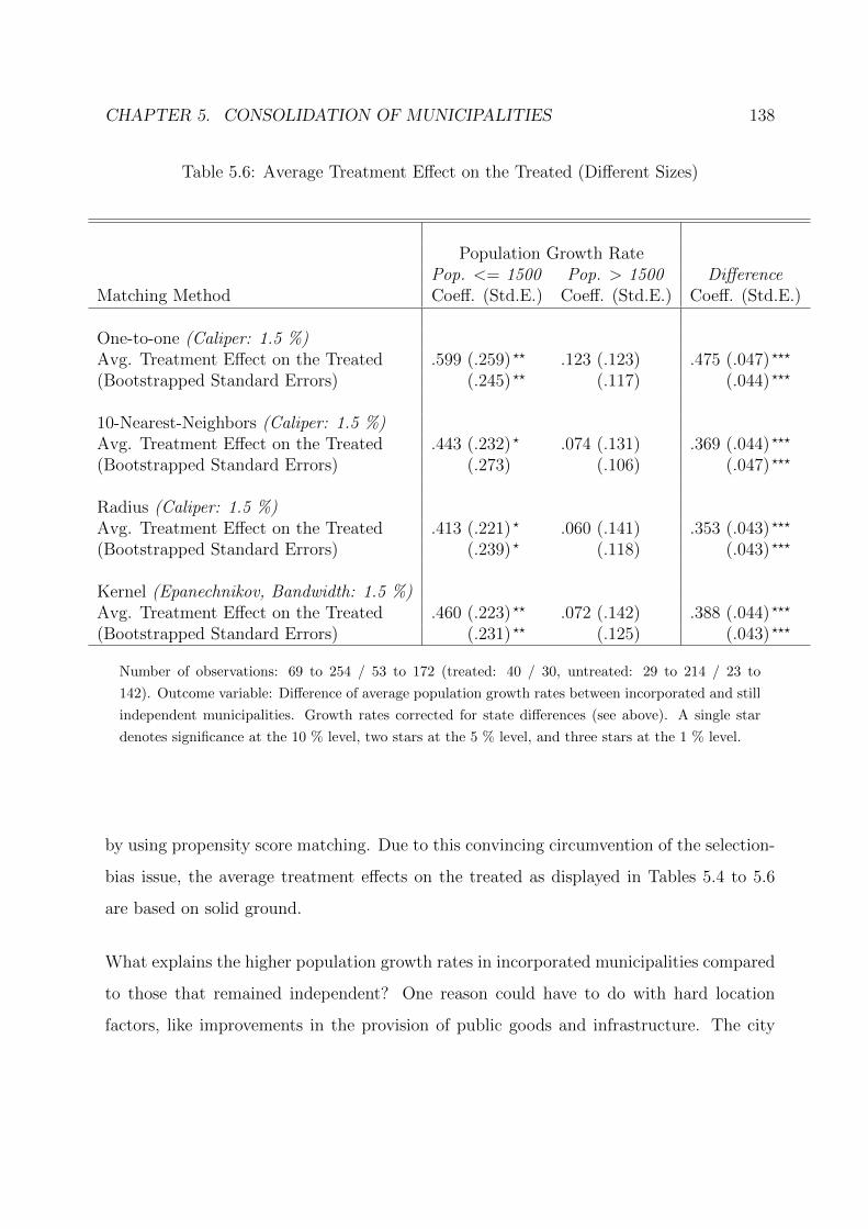
CHAPTER 5. CONSOLIDATION OF MUNICIPALITIES 138
Table 5.6: Average Treatment Effect on the Treated (Different Sizes)
Population Growth RatePop. <= 1500 Pop. > 1500 Difference
Matching Method Coeff. (Std.E.) Coeff. (Std.E.) Coeff. (Std.E.)
One-to-one (Caliper: 1.5 %)Avg. Treatment Effect on the Treated .599 (.259) ?? .123 (.123) .475 (.047) ???
(Bootstrapped Standard Errors) (.245) ?? (.117) (.044) ???
10-Nearest-Neighbors (Caliper: 1.5 %)Avg. Treatment Effect on the Treated .443 (.232) ? .074 (.131) .369 (.044) ???
(Bootstrapped Standard Errors) (.273) (.106) (.047) ???
Radius (Caliper: 1.5 %)Avg. Treatment Effect on the Treated .413 (.221) ? .060 (.141) .353 (.043) ???
(Bootstrapped Standard Errors) (.239) ? (.118) (.043) ???
Kernel (Epanechnikov, Bandwidth: 1.5 %)Avg. Treatment Effect on the Treated .460 (.223) ?? .072 (.142) .388 (.044) ???
(Bootstrapped Standard Errors) (.231) ?? (.125) (.043) ???
Number of observations: 69 to 254 / 53 to 172 (treated: 40 / 30, untreated: 29 to 214 / 23 to
142). Outcome variable: Difference of average population growth rates between incorporated and still
independent municipalities. Growth rates corrected for state differences (see above). A single star
denotes significance at the 10 % level, two stars at the 5 % level, and three stars at the 1 % level.
by using propensity score matching. Due to this convincing circumvention of the selection-
bias issue, the average treatment effects on the treated as displayed in Tables 5.4 to 5.6
are based on solid ground.
What explains the higher population growth rates in incorporated municipalities compared
to those that remained independent? One reason could have to do with hard location
factors, like improvements in the provision of public goods and infrastructure. The city

CHAPTER 5. CONSOLIDATION OF MUNICIPALITIES 139
Table 5.7: Balancing Property (Radius Matching)
Mean Mean % Bias % Bias t p > |t|Variable Treated Control Reduct.
log(Distance to Core City) 1.80 1.75 15.1 88.2 0.80 0.423log(Pop. 1961 Surr. Munic.) 7.29 7.30 -1.5 87.5 -0.09 0.929log(Pop. 1961 Core City) 11.4 11.3 13.4 62.8 0.92 0.358log(Area 1961 Surr. Munic.) 2.05 1.97 10.8 57.1 0.68 0.495log(Area 1961 Core City) 3.97 3.90 10.5 -36.0 0.67 0.506log(Debt 1966 Surr. Munic. (p.c.)) 5.27 5.25 8.4 61.7 0.58 0.562log(Debt 1966 Core City (p.c.)) 6.17 6.16 1.0 95.1 0.06 0.955Political Diff. Surr. Munic. 6.19 6.57 -2.1 89.7 -0.13 0.894Political Diff. Core City -10.3 -9.81 -5.1 70.3 -0.36 0.719Religious Difference 1961 9.00 10.0 -4.6 62.2 -0.30 0.767Dummy Schleswig-Holstein .075 .051 8.3 73.7 0.62 0.539Dummy Lower Saxony .1 .088 4.0 93.9 0.27 0.788Dummy North Rhine-Westphalia .038 .030 3.1 93.1 0.25 0.803Dummy Hesse .038 .028 6.5 -137.3 0.34 0.734Dummy Rhineland-Palatinate .325 .313 2.6 95.0 0.17 0.868Dummy Baden-Wurttemberg .275 .251 6.4 63.6 0.35 0.730Dummy Bavaria .15 .240 -25.2 -131.3 -1.43 0.154Dummy State Capital .125 .084 13.9 -150.8 0.85 0.397
Distance in kilometers, area in square kilometers, debt in Euro. The state of Saarland is missing due
to a lack of observations.
will probably be more willing to extend a subway or streetcar network to a city district than
to a municipality that is the same distance as the district from the city’s core, for example.
But other public goods and services may also contribute to the greater attractiveness of
an incorporated unit. This is the case when the public sector becomes more efficient by
exploiting economies of scale and is consequently able to increase the provision of goods and
services. Furthermore, mergers of municipalities can reduce the volatility in the provision
of public goods by absorbing revenue shocks due to an insurance effect. If these effects
CHAPTER 5. CONSOLIDATION OF MUNICIPALITIES 140
caused higher population growth rates, such would signal that the incorporation policy is a
success. Then municipalities would have lost their independent statuses that have actually
had potentials for increasing efficiency.
The location of housing programs is also potentially relevant. In the 1960s and 1970s, com-
muter towns were built within city borders to relieve pressure on the city’s core. Typically,
these were constructed in the outlying city districts, which may very well have included
some newly incorporated districts. Since these commuter towns were built in previously
sparsely populated areas, a high population growth rate could have resulted.
5.5 Conclusions
This chapter analyzes the impact of incorporations of city’s surrounding municipalities on
population growth in these units. To this end, the large reforms of the spatial adminis-
trative structure in Germany during the 1960s and 1970s are considered. To isolate the
effects on population growth, municipalities in the surrounding area of cities that remained
independent are compared with those that have merged with the adjacent core city.
To reduce a possible selection bias, a propensity score matching approach is used. We run
a probit regression that explains the probability of being incorporated. The distance of
the municipality to the center of the core city, its population, the geographic size of the
municipality, and state dummies are significant covariates that explain a notable part of the
variation. Given the predicted probability of consolidation, different methods of propensity
score matching are employed to match treated and untreated municipalities, with the intent
of making the two groups as similar as possible. Each of the methods employed proves able
to reduce the differences between treated and control municipalities to a large and sufficient
extent. The average treatment effect on the treated that is subsequently estimated, shows a

CHAPTER 5. CONSOLIDATION OF MUNICIPALITIES 141
significantly higher population growth rate for the incorporated municipalities. This holds
for all matching approaches, throughout which the effect remains constant. Adjusting the
calculations for different state growth rates confirms the results. Furthermore, the effect
appears to be larger for municipalities that were incorporated during the second part of
the reform period, which may be causal in this group to consist of stronger municipalities.
Moreover, the effect proves to be stronger for small municipalities.
The results contradict some theoretical predictions from the literature, according to which
citizens are opposed to mergers for political or fiscal reasons. These reasons may not only
result in no merger, but could also make the municipality less likely to attract new residents.
Other arguments seem more relevant, however. Among these may be improvements in the
connection between city and incorporated municipality (infrastructure) or a more efficient
provision of public goods in general. Also the location of past housing programs may play
a role.
It is left for future research to identify the effects of incorporation (or its absence) on
different economic indicators. In particular, location decisions of businesses may be influ-
enced by whether a possible location is situated within the borders of the core city or is
rather part of an independent surrounding municipality (driven by the level of taxation, for
example). Furthermore, the impact of consolidations on the political environment could
be analyzed, both as to election outcomes (due to a different composition of voters) and
political commitment.

CHAPTER 5. CONSOLIDATION OF MUNICIPALITIES 142
Appendix
Table 5.8: Descriptive Statistics (Incorporation <= 1972)
Variable Obs. Mean Standard Dev. Min Max
Population Growth Rate 521 .699 .874 -.339 10.0Pop. Growth Rate, State-Corr. 521 .460 .855 -.518 9.68Absolute Population Growth 521 1337 2450 -1236 26764Treatment 521 .142 .349 0 1Year of Incorporation 74 1971 1.38 1969 1972Distance to Core City 521 8.59 2.59 1.76 12.5Population 1961 Surr. Munic. 521 2164 3374 91 33290Population 1961 Core City 521 111031 161740 28725 1832346Area 1961 Surr. Munic. 521 10.5 9.32 .970 119Area 1961 Core City 521 59.6 54.5 9.65 747Debt 1966 Surr. Munic. (p.c.) 521 198 63.8 117 441Debt 1966 Core City (p.c.) 521 520 219 115 1271Political Diff. Surr. Munic. 521 6.02 17.1 -51.8 49.1Political Diff. Core City 521 -9.74 10.4 -65.0 20.7Religious Difference 1961 521 9.19 23.8 -103 79.4State Capital 521 .106 .308 0 1
Table shows also municipalities that have remained independent. The number of core cities in this
data set amounts to 62. Distance in kilometers, area in square kilometers, debt in Euro.

CHAPTER 5. CONSOLIDATION OF MUNICIPALITIES 143
Table 5.9: Descriptive Statistics (Incorporation > 1972)
Variable Obs. Mean Standard Dev. Min Max
Population Growth Rate 497 .713 .898 -.363 10.0Pop. Growth Rate, State-Corr. 497 .473 .877 -.560 9.68Absolute Population Growth 497 1465 3070 -1236 43100Treatment 497 .101 .301 0 1Year of Incorporation 50 1974 1.19 1973 1978Distance to Core City 497 8.84 2.36 2.49 12.5Population 1961 Surr. Munic. 497 2329 4112 91 50906Population 1961 Core City 497 123744 171829 28725 1832346Area 1961 Surr. Munic. 497 10.8 9.99 .970 119Area 1961 Core City 497 64.1 57.4 9.65 747Debt 1966 Surr. Munic. (p.c.) 497 198 66.9 101 441Debt 1966 Core City (p.c.) 497 520 212 115 1271Political Diff. Surr. Munic. 497 5.58 17.4 -51.8 49.1Political Diff. Core City 497 -9.98 10.8 -65.0 20.7Religious Difference 1961 497 8.71 23.3 -103 79.4State Capital 497 .101 .301 0 1
Table shows also municipalities that have remained independent. The number of core cities in this
data set amounts to 66. Distance in kilometers, area in square kilometers, debt in Euro.

CHAPTER 5. CONSOLIDATION OF MUNICIPALITIES 144
Table 5.10: Descriptive Statistics (Population <= 1500)
Variable Obs. Mean Standard Dev. Min Max
Population Growth Rate 356 .785 .925 -.363 6.36Pop. Growth Rate, State-Corr. 356 .555 .898 -.560 6.05Absolute Population Growth 356 658 875 -467 5193Treatment 356 .194 .396 0 1Year of Incorporation 69 1972 2.10 1969 1978Distance to Core City 356 8.68 2.49 2.68 12.5Population 1961 Surr. Munic. 356 787 378 91 1496Population 1961 Core City 356 96027 92032 28725 1085014Area 1961 Surr. Munic. 356 7.54 4.97 .970 34.0Area 1961 Core City 356 54.3 37.5 9.65 310Debt 1966 Surr. Munic. (p.c.) 356 201 68.1 109 441Debt 1966 Core City (p.c.) 356 500 213 115 1271Political Diff. Surr. Munic. 356 6.25 17.3 -51.8 46.0Political Diff. Core City 356 -10.1 10.0 -65.0 20.7Religious Difference 1961 356 7.04 23.2 -97.5 62.4State Capital 356 .101 .302 0 1
The number of core cities in this data set amounts to 50. Distance in kilometers, area in square
kilometers, debt in Euro.

CHAPTER 5. CONSOLIDATION OF MUNICIPALITIES 145
Table 5.11: Descriptive Statistics (Population > 1500)
Variable Obs. Mean Standard Dev. Min Max
Population Growth Rate 215 .685 .865 -.251 10.0Pop. Growth Rate, State-Corr. 215 .429 .862 -.429 9.68Absolute Population Growth 215 2816 4381 -1236 43100Treatment 215 .256 .437 0 1Year of Incorporation 55 1972 2.27 1969 1977Distance to Core City 215 7.99 2.69 1.76 12.4Population 1961 Surr. Munic. 215 4683 5512 1509 50906Population 1961 Core City 215 157252 231886 28725 1832346Area 1961 Surr. Munic. 215 15.4 12.7 2.33 119Area 1961 Core City 215 74.7 73.4 12.6 747Debt 1966 Surr. Munic. (p.c.) 215 191 59.2 101 441Debt 1966 Core City (p.c.) 215 548 228 115 1271Political Diff. Surr. Munic. 215 4.12 17.8 -39.2 49.1Political Diff. Core City 215 -9.87 11.3 -32.3 18.3Religious Difference 1961 215 11.4 23.3 -103 79.4State Capital 215 .102 .304 0 1
The number of core cities in this data set amounts to 54. Distance in kilometers, area in square
kilometers, debt in Euro.

CHAPTER 5. CONSOLIDATION OF MUNICIPALITIES 146
Table 5.12: Balancing Property (One-to-one Matching)
Mean Mean % Bias % Bias t p > |t|Variable Treated Control Reduct.
log(Distance to Core City) 1.80 1.78 7.4 94.2 0.39 0.698log(Pop. 1961 Surr. Munic.) 7.29 7.35 -6.8 42.2 -0.39 0.693log(Pop. 1961 Core City) 11.4 11.4 -0.4 99.0 -0.02 0.980log(Area 1961 Surr. Munic.) 2.05 1.99 7.8 69.0 0.46 0.644log(Area 1961 Core City) 3.97 3.96 0.5 93.4 0.03 0.975log(Debt 1966 Surr. Munic. (p.c.)) 5.27 5.26 4.7 78.7 0.33 0.740log(Debt 1966 Core City (p.c.)) 6.17 6.19 -3.9 80.2 -0.23 0.818Political Diff. Surr. Munic. 6.19 8.69 -13.9 33.1 -0.87 0.387Political Diff. Core City -10.3 -10.2 -1.5 91.4 -0.11 0.913Religious Difference 1961 9.00 9.87 -3.8 68.6 -0.23 0.819Dummy Schleswig-Holstein .075 .088 -4.3 86.2 -0.29 0.774Dummy Lower Saxony .1 .113 -4.0 93.9 -0.25 0.799Dummy North Rhine-Westphalia .038 .038 0.0 100.0 -0.00 1.000Dummy Hesse .038 .05 -8.5 -207.9 -0.38 0.701Dummy Rhineland-Palatinate .325 .313 2.7 95.0 0.17 0.866Dummy Baden-Wurttemberg .275 .238 9.8 43.6 0.54 0.590Dummy Bavaria .15 .163 -3.5 67.7 -0.22 0.829Dummy State Capital .125 .138 -4.2 23.9 -0.23 0.816
Distance in kilometers, area in square kilometers, debt in Euro. The state of Saarland is missing due
to a lack of observations.

CHAPTER 5. CONSOLIDATION OF MUNICIPALITIES 147
Table 5.13: Balancing Property (10-Nearest-Neighbors Matching)
Mean Mean % Bias % Bias t p > |t|Variable Treated Control Reduct.
log(Distance to Core City) 1.80 1.75 15.5 87.9 0.83 0.411log(Pop. 1961 Surr. Munic.) 7.29 7.29 -0.0 99.9 -0.00 0.999log(Pop. 1961 Core City) 11.4 11.3 12.0 66.5 0.83 0.407log(Area 1961 Surr. Munic.) 2.05 1.96 12.2 51.6 0.76 0.445log(Area 1961 Core City) 3.97 3.90 10.3 -33.5 0.66 0.510log(Debt 1966 Surr. Munic. (p.c.)) 5.27 5.25 6.4 70.8 0.44 0.663log(Debt 1966 Core City (p.c.)) 6.17 6.17 -1.0 94.9 -0.06 0.954Political Diff. Surr. Munic. 6.19 6.51 -1.8 91.5 -0.11 0.912Political Diff. Core City -10.3 -9.91 -4.1 76.0 -0.29 0.771Religious Difference 1961 9.00 9.71 -3.2 74.1 -0.21 0.836Dummy Schleswig-Holstein .075 .059 5.6 82.1 0.41 0.685Dummy Lower Saxony .1 .087 4.2 93.5 0.28 0.777Dummy North Rhine-Westphalia .038 .031 3.0 93.3 0.24 0.811Dummy Hesse .038 .027 7.1 -156.6 0.37 0.711Dummy Rhineland-Palatinate .325 .321 0.9 98.4 0.05 0.956Dummy Baden-Wurttemberg .275 .244 8.1 53.6 0.44 0.659Dummy Bavaria .15 .232 -22.9 -110.4 -1.31 0.192Dummy State Capital .125 .097 9.5 -71.7 0.57 0.573
Distance in kilometers, area in square kilometers, debt in Euro. The state of Saarland is missing due
to a lack of observations.

CHAPTER 5. CONSOLIDATION OF MUNICIPALITIES 148
Table 5.14: Balancing Property (Kernel Matching)
Mean Mean % Bias % Bias t p > |t|Variable Treated Control Reduct.
log(Distance to Core City) 1.80 1.75 14.3 88.8 0.76 0.450log(Pop. 1961 Surr. Munic.) 7.29 7.30 -0.9 92.1 -0.06 0.955log(Pop. 1961 Core City) 11.4 11.3 13.1 63.6 0.90 0.371log(Area 1961 Surr. Munic.) 2.05 1.98 10.1 60.0 0.63 0.532log(Area 1961 Core City) 3.97 3.91 9.8 -26.9 0.62 0.537log(Debt 1966 Surr. Munic. (p.c.)) 5.27 5.25 8.4 61.6 0.59 0.557log(Debt 1966 Core City (p.c.)) 6.17 6.16 1.4 92.7 0.08 0.933Political Diff. Surr. Munic. 6.19 7.76 -8.7 57.9 -0.55 0.582Political Diff. Core City -10.3 -9.54 -7.8 54.6 -0.55 0.581Religious Difference 1961 9.00 11.0 -8.7 29.0 -0.56 0.578Dummy Schleswig-Holstein .075 .054 7.3 76.6 0.54 0.588Dummy Lower Saxony .1 .090 3.2 95.0 0.22 0.827Dummy North Rhine-Westphalia .038 .035 1.1 97.4 0.09 0.929Dummy Hesse .038 .024 9.0 -228.4 0.48 0.628Dummy Rhineland-Palatinate .325 .320 1.1 97.9 0.07 0.943Dummy Baden-Wurttemberg .275 .244 8.3 52.7 0.45 0.652Dummy Bavaria .15 .234 -23.6 -116.9 -1.35 0.179Dummy State Capital .125 .083 14.0 -152.8 0.86 0.393
Distance in kilometers, area in square kilometers, debt in Euro. The state of Saarland is missing due
to a lack of observations.

CHAPTER 5. CONSOLIDATION OF MUNICIPALITIES 149
References
Abadie, A. and G. W. Imbens (2006): On the Failure of the Bootstrap for Matching
Estimators, NBER Technical Working Papers, 0325.
Alesina, A., R. Perotti, and E. Spolaore (1995): Together or Separately? Issues on the
Costs and Benefits of Political and Fiscal Unions, European Economic Review, 39,
751–758.
Alesina, A. and E. Spolaore (1997): On the Number and Size of Nations, Quarterly
Journal of Economics, 112 (4), 1027–1056.
Austin, D. A. (1999): Politics vs Economics: Evidence from Municipal Annexation, Jour-
nal of Urban Economics, 45, 501–532.
Blume, L. (2009): Regionale Institutionen und Wachstum. Sozialkapital, Kommunalver-
fassungen und interkommunale Kooperation aus regional- und institutionenokono-
mischer Perspektive, Institutionelle und Evolutorische Okonomik, Band 34, Metropo-
lis.
Bolton, P. and G. Roland (1997): The Breakup of Nations: A Political Economy Analysis,
Quarterly Journal of Economics, 112 (4), 1057–1090.
Brink, A. (2004): The Break-Up of Municipalities: Voting Behavior in Local Referenda,
Economics of Governance, 5, 119–135.
Caliendo, M. and S. Kopeinig (2008): Some Practical Guidance for the Implementation
of Propensity Score Matching, Journal of Economic Surveys, 22 (1), 31–72.
Filer, J. E. and L. W. Kenny (1980): Voter Reaction to City-County Consolidation Refe-
renda, Journal of Law and Economics, 23 (1), 179–190.

CHAPTER 5. CONSOLIDATION OF MUNICIPALITIES 150
Gadd, H., G. Hansson, and J. Mansson (2008): Evaluating the Impact of Firm Subsidy
Using a Multilevel Propensity Score Approach, CAFO Working Papers, Centre for
Labour Market Policy Research (CAFO), School of Business and Economics, Lin-
naeus University.
Kendall, M. G. (1952): The Advanced Theory of Statistics, Volume I, London.
Puttner, G. (1983): Handbuch der kommunalen Wissenschaft und Praxis: Kommunale
Aufgaben und Instrumente der Aufgabenerfullung: Bd. 3, Springer.
Rosenbaum, P. R. and D. B. Rubin (1983): The Central Role of the Propensity Score in
Observational Studies for Causal Effects, Biometrika, 70 (1), 41–55.
Sørensen, R. J. (2006): Local Government Consolidations: The Impact of Political Trans-
action Costs, Public Choice, 127, 75–95.
Wagener, F. (1969): Neubau der Verwaltung – Gliederung der offentlichen Aufgaben und
ihrer Trager nach Effektivitat und Integrationswert, Schriftenreihe der Hochschule
Speyer, 41, Berlin.

Chapter 6
Concluding Remarks
This book has analyzed the role of institutions in public finance, focusing on the issues of
revenue forecasting and the spatial administrative structure of municipalities. Chapter 2
analyzes the international differences in forecasting practices and shows that forecasting
performance depends on the institutional arrangement. The performance turns out to
improve with the degree of independence, but also hinges on the timing of the forecast and
the structure of the tax system. Chapter 3 looks into revenue forecasting in Germany and
widely confirms the unbiasedness and efficiency of the forecasts. Only with regard to tax
law changes and the term of office there appears to be some room to improve the forecasts.
In Chapter 4 we turn to local policies and provide evidence how the design of borders
impacts on local tax policy. Both the number of competitors and the size of a core city
in its agglomeration prove important. Chapter 5 analyzes the effects of reforms of spatial
administrative structures. Considering the reforms in Germany in the 1960s and 1970s, we
show that incorporated surrounding municipalities of core cities perform better in terms
of population growth than comparable municipalities that have remained independent.

CHAPTER 6. CONCLUDING REMARKS 152
What follows from the insights given in this book? And what is left for future research? The
purpose of this book is first of all to discover effects of institutions on the performance of the
public sector. Evidence is provided for the relevance of a number of institutions. There is,
however, still space left to analyze which political recommendations may follow. While the
main result of Chapter 2, that independent revenue forecasts are superior to public ones,
is clear in its implications, adjustments with respect to the other results cannot be easily
performed. The timing of forecasts has to fulfill the needs of the budgetary process and is
hence subject to this. This is even more the case with regard to the structure of the tax
system. One can hardly recommend that the importance of simple-to-forecast taxes should
be increased simply in order to be able to come up with more precise forecasts. However,
the results allow revenue forecasters to attribute forecast errors to certain circumstances
that they are exposed to. This may prevent replacing them with different forecasting
structures, a result that also follows from Chapter 3. The German Court of Auditors had
criticized the revenue forecasters in 2006 for being too optimistic in recent years. While
this may have been the case for a certain period, our analysis of forecasts over a period of
almost 40 years shows no significant bias. In this way the results take the pressure off the
forecasters.
Implications are somewhat different when local policies are considered. The results that are
derived in Chapter 4 explain a notable part of the variation in the level of local business
taxation in core cities of agglomerations. It seems natural to incorporate surrounding
municipalities into these cities or to consolidate them among themselves to improve the
fiscal position of the cities. However, analyzing the elasticity of tax bases regarding tax
rate changes and estimating the resulting revenue effects is beyond the scope of this book
and is left for future research. Furthermore, there are aspects besides the power to tax
businesses that also have to be mentioned where consolidations are considered. These
comprise aspects of political influence and tastes in public goods provision, for instance,
which can affect the attraction of citizens. This leads directly to the implications of Chapter

CHAPTER 6. CONCLUDING REMARKS 153
5. From this we learn that the incorporation into a city exerts a positive population growth
effect on the incorporated unit. However, it is again unclear whether this is an argument
in favor of incorporations. The interests of “long-established” citizens may differ from
those of potential new ones, as evidence in the literature on voting behavior in the case of
consolidations shows. To answer the question why these communes become more attractive
to citizens, a more in-depth analysis of this aspect has to be performed. Further research
must also be undertaken to identify effects of incorporations on other economic variables,
such as income levels or real estate prices.

Curriculum Vitae
12/2007 – 11/2011 Doctoral Student at the University of Munich,Junior Economist at the Ifo Institute forEconomic Research
10/2003 – 08/2007 Diploma in Economics,University of Bonn
2003 Abitur, Erzbischofliches Irmgardis-Gymnasium, Cologne
07.12.1983 Born in Attendorn, Germany