institute of transport and logistics studies - the university of sydney...

I T L S

INSTITUTE of TRANSPORT and LOGISTICS STUDIES The Australian Key Centre in Transport and Logistics Management

The University of Sydney Established under the Australian Research Council’s Key Centre Program.

WORKING PAPER ITLS-WP-05-08

Efficiency and Sample Size Requirements for Stated Choice Studies By Michiel CJ Bliemer* & John M Rose *Assistant Professor Transportation Modeling Delft University of Technology Faculty of Civil Engineering and Geosciences Transport and Planning Section Delft, The Netherlands Adjunct Professor Institute of Transport & Logistics Studies * corresponding author ISSN 1832-570X April 2005

NUMBER: Working Paper ITLS-WP-05-08 TITLE: Efficiency and Sample Size Requirements for Stated

Choice Studies ABSTRACT: Stated choice (SC) experiments represent the dominant data

paradigm in the study of behavioral responses of individuals, households as well as other organizations, yet little is known about the sample size requirements for models estimated from such data. Current sampling theory does not adequately address the issue and hence researchers have had to resort to simple rules of thumb or ignore the issue and collect samples of arbitrary size, hoping that the sample is sufficiently large enough to produce reliable parameter estimates. In this paper, we demonstrate how to generate efficient designs (based on D-efficiency and a newly proposed sample size S-efficiency measure) using prior parameter values to estimate multinomial logit models containing both generic and alternative-specific parameters. Sample size requirements for such designs in SC studies are investigated. In a numerical case study is shown that a D-efficient and even more an S-efficient design needs a (much) smaller sample size than a random orthogonal design. Furthermore, it is shown that wide level range has a significant positive influence on the efficiency of the design and therefore on the reliability of the parameter estimates.

KEY WORDS: Stated Choice Experiments, D-optimality, D-error,

Sample Size, Multinomial Logit AUTHORS: Michiel CJ Bliemer & John M Rose CONTACT: Institute of Transport and Logistics Studies (Sydney) The Australian Key Centre in Transport and Logistics

Management, (C37) The University of Sydney NSW 2006 Australia

Telephone: +61 9351 0071 Facsimile: +61 9351 0088 E-mail: [email protected] Internet: http://www.itls.usyd.edu.au DATE: April 2005

Efficiency and Sample Size Requirements for Stated Choice Studies Bliemer & Rose

1

1. Introduction Stated choice (SC) methods are not new. Since first being introduced ([0] and [0]), SC methods have been used in such diverse fields as marketing, transport and environmental and health economics. In the process, SC methods have become the dominant data paradigm in the study of behavioral responses of individuals, households as well as other organizations. Within the health economics literature, SC methods have been used to measure the willingness to pay to reduce risk of fractures [0], to estimate the preferences for the introduction of new vaccinations (e.g., [0]), to evaluate the prescribing decisions of Doctors [0] and to determine the likely public responses to health care [0-0]. Despite recently being called into question [0-0], SC methods have remained the dominant method for revealing individuals preferences as well as marginal rates of substitution between attributes (i.e., willingness to pay) due to the ability of such methods to mimic, realistically, decisions made in actual markets [0]. Typically, SC experiments involve sampled respondents completing one or more choice tasks in which they are asked to choose from amongst a number of either labeled or unlabeled alternatives defined on a number of attribute dimensions, each in turn described by pre-specified levels drawn from some underlying experimental design. Since first being introduced to the literature, research on SC theory and methods has centered on identifying sources of cognitive burden placed upon respondents undertaking SC tasks (e.g., [0-0]) as well as reducing the cognitive load placed on those same respondents (e.g., [0-0]). These studies have tended to focus on within respondent information processing and cognition and have not specifically addressed methods of identifying the minimum sample size requirements in accordance with specific criteria of performance. Identifying methods for reducing the number of respondents required for SC experiments is important for many studies given increases in survey costs. Such reductions, however, must not come at the cost of a lessening in the reliability of the parameter estimates obtained from models of discrete choice. For whilst SC studies provide a realistic means of capturing decisions made in real markets, reliability in the parameter estimates is attained through the pooling of choices made by different respondents. For example, a typical SC experiment might require the pooling of choices made by 200 respondents, each of whom is observed to make eight choices, thus producing a total of 1600 choice observations. Several authors, publishing mainly in the marketing literature, have examined various methods to reduce the number of sampled respondents required to complete choice tasks whilst maintaining reliability in the results generated (e.g., [0-0]). The usual method of reducing the number of sampled respondents in SC experiments conducted in health studies appears to be using orthogonal fractional factorial experimental designs with respondents assigned to choice situations via either a blocking variable (e.g., [0]) or via random assignment (e.g., [0]). Through the use of larger block sizes (i.e., each block has a larger number of choice situations) or by the use of a greater number of choice situations being randomly assigned per respondent, analysts may decrease the number of respondents whilst retaining a fixed number of


2

choice observations collected. It should be noted, however, that whilst such strategies reduce the number of respondents required for SC experiments, they also reduce the variability observed in other covariates collected over the sample. Yet despite practical reasons to reduce survey costs, particularly through reductions in the sample sizes employed in SC studies, questions persist as to the minimum number of choice observations required to obtain reliable parameter estimates for discrete choice models estimated from SC data. Unfortunately, current sampling theory does not address the issue of minimum sample size requirements in terms of the reliability of the parameter estimates produced. Rather, sampling theory as applied to choice modeling is designed to minimize the error in the choice proportions of the alternatives under study. Given that the choice proportions in SC experiments are determined not only over respondents, but over choice situations, sampling theory as it exists is inadequate to determine what sample sizes choice modelers collecting SC data should be employing. Rather than rely on current sampling theories, we demonstrate how it is possible to determine the likely asymptotic efficiency (i.e., reliability) of the parameter estimates of discrete choice models estimated from SC data at different sample sizes. The article is organized as follows: The next section reviews the current theory of calculating the minimum sample size requirements for SC studies after which we derive the multinomial logit (MNL) model, used throughout this paper. Next, we discuss the theory on the optimization of SC experiments. In the following section, we provide a numerical example, showing the results for three different designs; an orthogonal, D-optimal and what we have termed S-optimal (sample size optimal) design. Then, we demonstrate the influence various design dimensions (e.g., the number of choice situations, number of levels, etc), have upon the sample size requirements of SC experiments. Finally, we draw conclusions and suggest recommendations for future research.

2. Sampling Theory for Stated Choice Experiments For studies of discrete choice, several sampling strategies exist, each of which provide for different methods to calculate the minimum sample sizes required. The three most dominant sampling strategies include simple random sampling (SRS), exogenous stratified random sampling (ESRS) and choice based sampling (CBS) (for a detailed description of these and alternative sampling strategies, see [0] or [0]). CBS is a sampling strategy used only in studies where the choice shares for a population are known a priori, as in revealed preference (RP) data. CBS involves under or over sampling on the endogenous choice variable so that rarely chosen alternatives are disproportionately represented in the data compared to their occurrence in the population. This allows for estimation of parameter estimates for those alternatives that could not otherwise be estimated given the lack of observations from which estimates may be derived. Given that CBS is not used in SC studies, we do not discuss this sampling strategy further in this paper. We now outline the calculations used to determine the minimum sample size requirements under the SRS and ESRS sampling strategies.


3

2.1 SRS sampling strategies For simple random samples (SRS), the minimum acceptable sample size, N, is determined by the desired level of accuracy of the estimated probabilities, p . Let p be the true choice proportion of the relevant population, a be the level of allowable deviation as a percentage between p and p, and γ be the confidence level of the estimations such that ˆPr( )p p ap γ− ≤ ≥ for a given N. The minimum sample size is defined as (see [0]):

( ) 21 12 21 ,

qN

paαΦ− ≥ − (1)

where 1 ,q p≡ − 1 ,α β≡ − and ( )1 121 α−Φ − is the inverse cumulative distribution

function of a standard normal evaluated at 121 .α−

Equation (1) is used to determine the minimum sample size required assuming that the analyst possesses only a single choice observation for each sampled respondent. Nevertheless, the usual practice in SC studies is for sampled respondents to complete multiple treatment combinations (in the form of choice situations) of the design over the course of the experiment. Denoting the number of treatment combinations assigned to each sampled individual as S, the minimum sample size in terms of sampled respondents N, taking into account the multiple responses per individual, becomes

( ) 21 122 1 .

qN

Spaα− ≥ Φ − (2)

The total number of choice observations required is therefore .N S⋅ Equation (2) only holds if choices made by sampled respondents are independent over decision tasks (see [0]). Interdependence over observations means that one cannot increase the number of choice situations shown to each decision maker in order to decrease the number of decision makers required to be sampled (unfortunately this cannot be tested a priori). Further, reductions in the number of sampled respondents result in corresponding decreases in the variability of socio-demographic characteristics and contextual effects observed within the sample, which in turn is likely to pose problems at the time of model estimation if such effects are to be included in within the model.

2.2 ESRS sampling strategies With exogenous stratified random sampling (ESRS), the population is first divided into G mutually exclusive groups, each representing a proportion of the total population,

.gW As discussed in [0], the basis for creating the groups can be any characteristic common to the population (e.g., age, income, location, gender, etc.) with the exception of choice. That is, the analyst cannot form groups based upon the observed choice of


4

alternative as would occur with choice based sampling. To maintain randomness within the sample (a desirable property if one wishes to generalize to the population), a random sample is drawn within each stratum. The sample sizes drawn within each stratum need not be equal across stratums. To calculate the sample size for a stratified random sample, the analyst may either (a) apply Equation (2) to establish the minimum total sample size and subsequently partition the total sample size into the G groups or (b) apply Equation (1) to each stratum and sum the sample sizes calculated for each stratum to establish the total sample size. Strategy (a) will produce smaller minimum sample sizes than strategy (b); however the analyst must recognize the effect on the acceptable error in using strategy (a) as the accuracy of the results when using strategy (a) will be related to the overall proportion whilst the accuracy of the results for strategy (b) will be relative to the within-group proportions [0]. Strategy (a) suggests the use of the overall population proportions to first derive the minimum sample size after which, the sample sizes of each of the G groups is determined either by (i) dividing the total sample size into the G groups equally, or (ii) apportioning the total sample size in accordance with the observed division of strata. Strategy (b) on the other hand requires the calculation of minimum sample size requirements for each of the strata, G, and summing the derived minimum samples sizes for each strata to calculate the overall minimum sample size required for the study.

2.3 Sampling for Stated Choice Studies Neither SRS nor ESRS sampling strategies are appropriate for SC studies. Both equations (1) and (2) assume a priori knowledge of the choice proportions. For RP studies, these proportions may be known in advance, and if not known, may at least be inferred to some level of accuracy. For SC studies, the choice proportions are determined over choice situations completed by numerous respondents, and as such, may not readily be known in advance. Further, p in Equations (1) and (2) generally represents the choice proportions for the most important alternative under study. For SC experiments, this alternative may not currently exist within real markets, making a determination of p, a priori, difficult, if not impossible. Further yet, many SC experiments conducted, employ unlabeled or generic designs. In unlabeled choice experiments, respondents are asked to choose from amongst a number of hypothetical alternatives that are defined solely by the attributes and attribute levels of the alternatives, as determined by the underlying experimental design (i.e., the names of each of the alternatives do not meaningfully convey information (usually) beyond the order of presence of each of the alternatives within each choice situation). Whilst it is possible to assume that each alternative will be chosen an equal number of times over the experiment (i.e., 1/p J= where J is defined as the number of alternatives), this assumption will hold only if (i) each alternative is dominant, as defined by the attributes and attribute levels, an equal proportion of times across choice situations or (ii) each alternative is equally preferred over all choice situations. In situation (i), no information is captured from the experiment and in situation (ii) the choice of an alternative will likely be random, hence making the results of the experiment suspect. Fractional factorial designs are unlikely to result in experiments in which alternatives will be chosen an equal proportion of times. Clearly, therefore, Equation (2) is inappropriate to


5

calculate the sample size requirements for both unlabeled and labeled choice experiments.

3. Multinomial logit model The multinomial logit (MNL) model is the most widely used model for predicting choice behavior of people in discrete choice situations. This well-known model will serve as the basis for our analysis and will be described here mainly to introduce the various concepts that are necessary to understand in reading the remainder of the paper. The MNL model has as its basis random utility theory (RUT), which is used to explain choice behavior. In a choice situation with multiple alternatives (e.g., choosing between different health care products), it is assumed that one will choose the alternative that generates the highest utility. Suppose there are J alternatives, and each alternative j has its own utility .jU Within the RUT framework, utility will be comprised of both an

observed, jV , and an unobserved component, ,jε such that

, 1, , .j j jU V j Jε= + = K (3)

Each alternative will be characterized by a set of attributes (e.g., efficacy, duration of action, indications). Each alternative is assumed to have a corresponding ‘global’ utility made up of the marginal (dis)utilities associated with each of the attribute dimensions (referred to as part-worths in some literature). Within RUT, these attribute related marginal (dis)utilities are reflected as ‘taste’ weights (i.e., the unknown population parameters). For the MNL model, these parameters may be specified as either generic or alternative-specific. If a parameter is generic, then the weight associated with the corresponding attribute is the same for each alternative that attribute appears in. For example, the taste weights or parameters for an attribute, duration of action, could be the same between different AIIRA+ drug alternatives. On the other hand, the taste weights attached to the reduction at starting dose to systolic BP between different drug alternatives may be different, such that the marginal utility for one drug given a reduction in systolic BP (as measured in mm Hg) is much greater than that given a similar reduction for another alternative. Consider a certain alternative j. Suppose this alternative has *K attributes with generic parameters and jK attributes with alternative-specific parameters. The observed utility,

jV , may be written as

*

*

1 1

, 1, , ,jKK

j k jk jk jkk k

V x x j Jβ β= =

= + ∀ =∑ ∑ K (4)

where *

jkx denotes a generic attribute with associated generic parameter *,kβ and jkx denotes an alternative-specific attribute with associated alternative-specific parameter

.jkβ The unobserved component of the model, jε , is assumed to be a stochastic variable. In the MNL model, these stochastic variables for all alternatives are assumed to be


6

independently and identically extreme value type I distributed. It has been shown by McFadden [0] that the probability of choosing alternative j, which we denote by ,jP is given by

1

exp( ), 1, , .

exp( )

jj J

ii

VP j J

V=

= ∀ =

∑K (5)

Hence, given the attribute values and corresponding parameters for each alternative, it will be possible to predict the overall ‘attractiveness’ of each alternative, as well as the probability that each alternative will be chosen. Unfortunately, it is unlikely that the analyst will know the population parameters *( , )β β prior to undertaking the study. It therefore becomes necessary to obtain these parameters from data. In order to estimate the parameters, the analyst may collect data using one of two different data paradigms (or if more advanced models are to be used – in particular the nested logit model – both data types can be combined within one study). The first data paradigm relies on the collection of revealed preference (RP) data. Revealed preferences consists of data collected on the choices made by those operating in real markets (i.e., choices made in real life choice situations). The second data paradigm, data collected on stated preference (SP), of which SC data is a specific case, is data that is collected on choices made in hypothetical situations usually presented to sampled respondents in some form of survey. Given that RP data is collected on the events occurring in real markets, the data will usually provide the analyst with a high degree of reliability as well as validity. Unfortunately, RP data is limited in that it is restricted to the current technological frontier. That is, RP data can only be gathered on the alternatives, attributes and attribute levels existing on the market place at the time the data is collected. Stated preference data, however, allows the analyst to gather information on contexts that may or may not necessarily currently exist and therefore allows an exploration of new likely situations that could arise in the future. As such, SP (or SC) data can be powerful in predicting choice behavior on a wider range of attribute values as well as allowing for an examination of the impact currently non-existent alternatives will have upon the choices made by those operating in real markets. For example, how will a new generic drug affect the preference for existing drugs within a market? The design of these experiments will be the topic of the next section.

4. Design of stated choice experiments In a stated choice (SC) experiment, sampled respondents are presented with a series of hypothetical choice situations in each of which they asked to select the alternative that they find most attractive, given the attribute levels of all alternatives present within each specific choice situation. Stated choice experiments may be either unlabeled or a labeled. As discussed in Section 2, in a labeled choice experiment, each alternative is given a branded name, which provides some meaningful reference of distinction from the other alternatives present within the choice task. In an unlabeled choice experiment, the alternatives in the experiment are given generic names such that each alternative


7

cannot be associated with any specific branded product (for example Alternative A, B, C, etc.). Depending on whether an experiment is labeled or unlabeled, the analyst may specify that the parameters be either generic of alternative-specific. As unlabeled experiments are not brand specific, it is necessary that the parameters related to the alternatives of such experiments be estimated as generic. For labeled choice experiments, the parameters may be specifically related to each brand, and hence be estimated as alternative-specific, however, it is also possible that (some of) the parameters of labeled choice experiments be estimated as generic parameter estimates (e.g., the parameter for price may be different for different brands, hence reflecting different price sensitivities, whilst a parameter associated with the number of clinical trials supporting each brand might be generic, indicating that the same weight is attached to this attribute independent of the brand). Underlying each SC experiment is what is known as an experimental design. An experimental design consists of S different choice situations. In each choice situation, s , different combinations of attribute levels are shown to the respondent and the respondent is asked to select the best alternative. The levels for the attributes are typically selected from a fixed set of possible values. Let *

jkL be the set of possible

levels of generic attribute k of alternative j and let jkL denote the set of levels for alternative-specific attribute k of alternative j. The problem then becomes to locate a ‘good’ design *( , )x x with * *

jks jkx L∈ and jks jkx L∈ for all 1, , ,s S∈ K satisfying a number of possible analyst-imposed constraints. One such constraint typically imposed is that of attribute level balance, which states that for each attribute, all levels are represented an equal number of times over the S choice situations. In the past, two main approaches have been considered for finding a ‘good’ design: (a) finding an orthogonal design, and (b) finding a D-optimal design. The first design approach aims to minimize the correlations between attribute levels shown to the respondents, while the second approach aims to minimize the (co)variances in the parameter estimates assuming some prior knowledge of the parameter values. Clearly, it is possible to combine both approaches in creating a design. Nevertheless, recent research has shown (e.g., [0-0],[0-0]) that D-optimal designs can provide (much) better parameter estimates than orthogonal designs, assuming that prior knowledge is available, at much smaller sample sizes. For this reason, we will mainly focus on D-optimal designs that are statistically efficient. The statistical efficiency of a design can be expressed by a single term, which the literature has termed D-error. The D-error of an experimental choice design will be low if the asymptotic (co)variances of the parameter estimates are low and high of these (co)variances are high. As such, a low D-error indicates a more efficient design. Let NΩ denote the asymptotic (co)variance matrix for the parameter estimates based on N respondents. This is a symmetric matrix of dimension equal to the number of parameters to estimate. The total number of (generic and alternative-specific) parameters to estimate is * .jj

K K K= + ∑ The D-error is computed as the determinant of 1Ω

(assuming just a single respondent) to the power of the inverse of the number of parameters to be estimated (for scaling purposes),


8

( )1/1D-error det .K= Ω (6)

The design yielding a minimum D-error is called a D-optimal design. Finding a D-optimal design is typically a difficult problem, as there exist exponentially many designs with different combinations of attribute levels. Therefore, instead of using the term D-optimal design, it is more appropriate to use the term D-efficient design for a design with a low D-error, as we cannot guarantee finding a design with the lowest D-error. Two types of D-optimal designs have been discussed in the literature, these being pD -

optimal and zD -optimal designs. Assuming that the asymptotic (co)variance matrix is computed based on some prior non-zero parameter values (obtained from, e.g., literature or pilot studies), then the design with lowest D-error is termed a pD -optimal design. If no prior information is available (even if only on the expected sign of the parameter estimates) and the asymptotic (co)variance matrix is computed assuming that all parameters are simultaneously equal to zero, then the design with the lowest D-error is called a zD -optimal design. Common sense suggests that having information can potentially result in more efficient designs than having no information. In the case of a labeled choice experiment, there is a clear relationship between a zD -optimal design (having no prior information) and an orthogonal design, as shown in [0]. In this paper we will focus on pD -optimality. The most common method of estimating the parameters from an MNL model, *( , )β β ,

is to find *ˆ ˆ( , )β β through maximizing the log-likelihood function:

*

* *

( , ) 1 1

ˆ ˆ( , ) argmax ( , ) log ,n

N J

jsn jsn s S j

L y Pβ β

β β β β= ∈ =

= = ∑ ∑ ∑ (7)

where nS is the set of choice situations respondent n is faced with, jsny equals one if

respondent n chooses alternative j in choice situation s and zero otherwise, and jsP is the choice probability for alternative j in choice situation s, using Equation (5) with the attribute levels of choice situation s and the (estimated) parameter values. Although it is possible to show respondents different choice situations (this may be done by blocking the design or by random assignment of different choice situations to different respondents), in the theory of D-optimality, it is common to assume a single design, and hence, 1, , .nS S= K McFadden [0] has shown for the generic case that the maximum

likelihood estimates *ˆ ˆ( , )β β are asymptotically normally distributed with means equal to the true parameter values and a covariance matrix NΩ equal to the negative inverse of the Fisher information matrix. Therefore, assuming that the prior parameter values are the true parameter values and noting that the parameter estimates converge to the true parameter values, it becomes a relatively straightforward task to compute the Fisher information matrix based on the prior parameter values, *( , )β β , and from this, the pD -error. The Fisher information matrix consists of the second derivatives of the log-


9

likelihood function. Assuming that all respondents face the same choice situations, taking the second derivatives yields the following expressions (see [0]):

1 2 2

1 2

2 ** * *

* *1 1 1

( , ),

S J J

jk s js jk s ik s iss j ik k

LN x P x x P

β ββ β = = =

∂ = − − ∂ ∂ ∑∑ ∑ (8)

1 1 1 1 2 2

1 1 2

2 ** *

*1 1

( , ),

S J

j k s j s j k s ik s iss ij k k

LN x P x x P

β ββ β = =

∂ = − − ∂ ∂ ∑ ∑ (9)

( )

1 1 2 2 1 2

1 1 2 2

1 1 2 2 1 2

1 22 *1

1 21

, if ;( , )

1 , if .

S

j k s j k s j s j ss

Sj k j k

j k s j k s j s j ss

N x x P P j jL

N x x P P j j

β ββ β

=

=

≠∂ = ∂ ∂ − − =

∑

∑ (10)

Note that these second derivatives are independent of the experiment outcomes y. If a model is estimated using only generic parameters, then only Equation (8) is required (which is similar to the equation stated originally by McFadden [0] and reported in several other sources (e.g., [0-0], [0]) to obtain the asymptotic (co)variance matrix. If only alternative-specific parameters are to be estimated, then only Equation (10) is required (which is same as the equation stated in [0]). Software packages such as NLOGIT produce the same results when using Monte Carlo simulation and computing the Fisher information matrix by means of numerical approximation. However, using these analytical equations it becomes no longer necessary to conduct Monte Carlo simulations, as it is possible to directly locate the asymptotic (co)variance matrix using the above equations. By implicitly assuming that the prior parameter values are the true parameter values, it becomes possible to derive statistically efficient designs. While this seems a very strong assumption, we note that any information on the parameter values (e.g., the signs) can represent a significant contribution towards improving the efficiency of a design. Typically, there will exist some information available to the analyst, or alternatively, some indication (even if only the likely direction of the parameter) might be obtained from focus groups or pilot studies. Sensitivity analysis on the assumed priors may give clues on the stability of the efficiency. Assuming that the prior parameters are correct, let *( , )Nse β β denote the vector of asymptotic standard errors of the generic and alternative-specific parameter estimates for a study with sample size N. These are simply the square roots of the diagonal elements of matrix NΩ . Let the Fisher

information matrix with N respondents be denoted by *( , ).NI β β Since * *

1( , ) ( , ),NI N Iβ β β β= ⋅ it holds that ( ) ( )1 1* *11( , ) ( , )N N NI Iβ β β β

− −Ω = = 1

1,N= Ω

such that

** 1( , )

( , ) .N

sese

Nβ β

β β = (11)


10

Hence, the asymptotic standard errors provide diminishing improvements (decreases) for larger sample sizes. Summarizing, given a SC experimental design and prior parameter values, it is possible to determine the asymptotic standard errors for any sample size. An efficient design based on good priors may provide more useful data and yield more reliable parameter estimates (i.e., parameter estimates with smaller asymptotic standard errors) with fewer respondents. As such, the required sample size in terms of the number of respondents may be (much) smaller if a design is more efficient (or similarly, more accurate parameter estimates can be obtained with a fixed sample size). The next section discusses the issue of sample sizes in more detail.

5. Sample size Within the literature, there does not appear to exist a formula for computing the required sample size in case of performing stated choice experiments. As discussed in Section 2, the current sampling theory as exists does not directly address the issue of minimum sample size requirements in terms of the reliability of the parameter estimates produced (see for example, [0-0]). Rather, sampling theory as applied to choice modeling is designed to minimize the error in the choice proportions of the alternatives under study. As such, sampling theory as it exists with regards to SC experiments is only applicable to the collection of RP choice data. The previous section demonstrated how it is possible for the analyst to determine the asymptotic standard errors for any arbitrary SC experimental design given any sample size, N. The procedure outlined in Section 4 is useful for obtaining an indication regarding the sample size requirements for the model estimation. Furthermore, it will give insight into the efficiency of the design with respect to each of the parameters to be estimated. As will be shown by way of a numerical example, a D-optimal design may result in some parameters being estimated with much higher levels of reliability (i.e., lower standard errors) than others, due to the use of a single ‘global’ measure of efficiency. An interesting proposition therefore, is to consider a more egalitarian approach that will minimize the sample size required for the experiment in such a way that it will improve the level of reliability of those parameters with high standard errors. One appealing approach is to use the asymptotic t-ratios assess the efficiency of the experiment. While the D-error only indicates overall combined efficiency, the asymptotic t-ratios give information about the efficiency of each of the parameters individually. Further, unlike the asymptotic standard errors, the asymptotic t-ratios are scaled in accordance to the magnitude of the attributes that they correspond with. We call this approach the S-efficiency approach. Given a certain sample size, the asymptotic t-ratios based on prior parameter estimates are calculated by dividing the prior parameters with their corresponding standard errors. A theoretical minimum sample size for a parameter estimate to be statistically significant can then be determined. For example, consider generic parameter *

kβ . Then the asymptotic t-ratio should be larger than 1.96 in order to state with 95 percent certainty that it is statistically significant. That is,


11

*

* 1.96.( )k

N kseβ

β≥ (12)

Substituting Equation (11) into (12) and rearranging terms, yields

2*1

*

1.96 ( ).k

k

seN

ββ

⋅≥

(13)

A similar equation holds for the alternative-specific parameters. We can view the sample size requirement stated in Equation (13) as a theoretical lower bound for finding a statistically significant parameter estimate for that parameter. Different parameters may have different lower bounds. Parameters with high lower bounds will be more difficult to estimate than parameters with low lower bounds. In case we would like to find the minimum theoretical sample size for which all parameters are statistically significant, then we would probably prefer to change the design in such a way that the parameters that are difficult to estimate obtain more information from the design in order to decrease its standard error. In other words, we may prefer to have all parameter estimates in the same range with their asymptotic t-values such that all parameters get equal attention in the design. We term a design that minimizes the sample size needed for all parameters to be statistically significant an S-efficient design. Instead of changing the design itself given the attribute levels to choose from, it is possible to change other aspects of the experiment. For example, it may be possible to change the attribute levels (i.e., the number of levels and/or the level range) of the design or change the number of choice situations presented to each individual respondent. In the next section we will present some results using a numerical example of a design that is optimized for standard errors and sample size. We will show that the design may be improved by increasing the level range, having fewer levels, and focusing on the asymptotic t-ratios instead of on just the D-error.

6. Numerical analysis 6.1 D-efficient and S-efficient designs In order to illustrate the theory of efficient designs and discuss issues of sample size, we will consider the following discrete choice problem. Suppose there are two alternatives, each having several generic and alternative-specific attributes. The first alternative has two generic attributes and two alternative-specific attributes. The second alternative has the same two generic attributes, an alternative-specific constant, and two alternative-specific attributes. This is stated in the following two utility functions:

* * * *1 1 11 2 12 11 11 12 12 , 1, ,12,s s s s sV x x x x sβ β β β= + + + = K (14)

* * * *

2 21 1 21 2 22 22 22 23 23 , 1, ,12.s s s s sV x x x x sβ β β β β= + + + + = K (15)


12

In total, there are seven parameters to estimate, whilst there are eight attributes that change attribute levels. The constant, 21,β has a fixed attribute level of one. Within the SC experiment, the eight attributes can take on different levels over the different choice situations shown to respondents. Let us assume that each attribute can take on one of three levels and that each sampled respondent will review twelve choice situations. Assume that the attributes may take on the following levels: * *

11 21 22 2,4,6,L L L= = = * *12 22 21 1,3,5,L L L= = = and 12 23 4,6,8.L L= = Following common practice, we

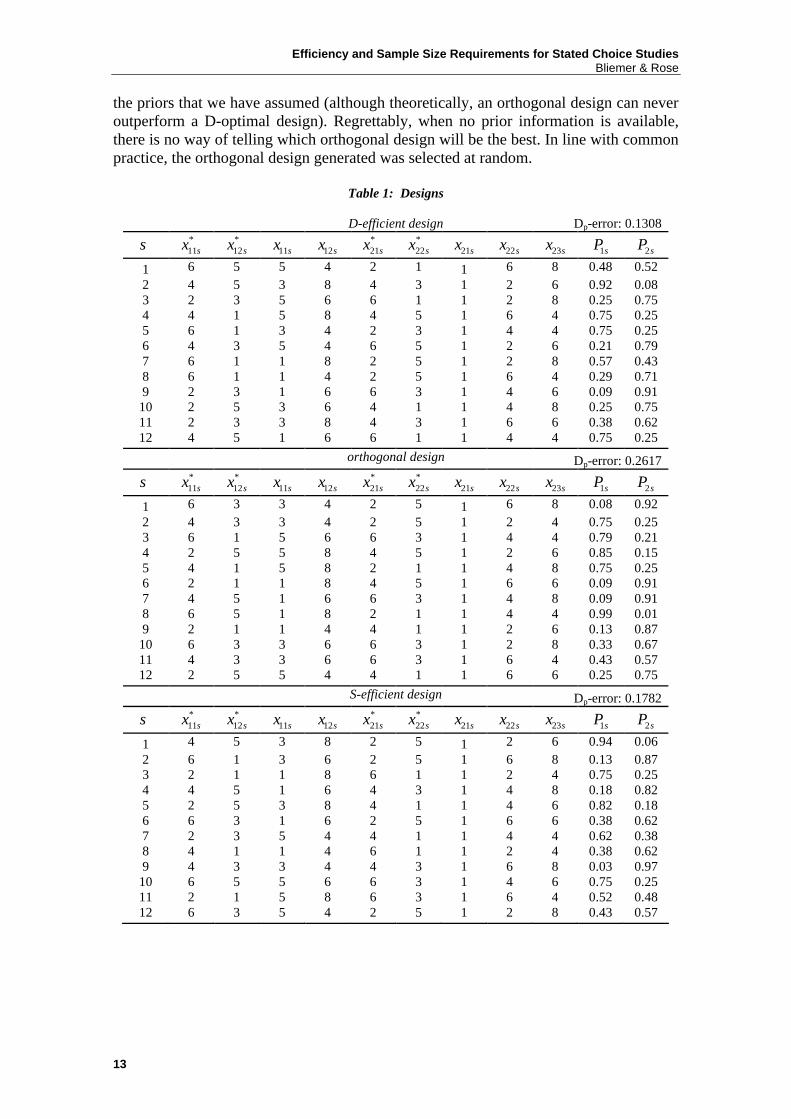
constrain ourselves to balanced designs (although such a constraint may result in the generation of a sub-optimal design). We will examine three different design types: (a) a D-efficient design, (b) an orthogonal design, and (c) an S-efficient design. The D-efficient design aims to minimize all (co)variances of all parameter estimates, the orthogonal design minimizes to zero the correlations between the attribute values, and the sample size efficient design aims to minimize the sample size needed to obtain statistically significant parameter estimates (i.e., all asymptotic t-ratios must be greater than 1.96). The three designs are presented in Table 1. The first and last designs assume prior knowledge of the parameter values. The used priors are stated in Table 2. In all designs the constant is ignored when computing the D-error, the correlation coefficients, or the minimum sample size (the constant is not ignored when computing the probabilities in the logit model. It is merely eliminated at the final stage when computing values such as the D-error for judging the efficiency or orthogonality of a design). The constant is typically ignored in these kind of studies, since usually the constant is of less importance to the researcher (indeed the constant is often considered meaningless in stated choice experiments as it is based on the choice shares over the hypothetical situations, S). Further, in many SC studies, it is often the ratios of two parameter values (e.g., to derive willingness to pay) that is of primary importance. Therefore, in calculating the D-errors for each design we ignore the row and column for the constant in the asymptotic (co)variance matrix when computing the determinant in Equation (6). In calculating the minimum sample size, the constant need not be statistically significant. The D-error of the orthogonal design is approximately twice as high as the D-error of the D-efficient design. This means roughly that on average the standard error of the parameter estimates using the orthogonal design will be 2 times larger than the average standard error of the estimates using the D-efficient design. This in turn means that approximately twice as many observations using the orthogonal design are required in order to obtain the same values for the standard errors. This demonstrates that information on prior parameter estimates can clearly help significantly in making a more efficient design. In cases where one has no information on the parameter estimates whatsoever, it is common practice to assume that the prior parameter estimates are all equal to zero. As mentioned in [0], when only alternative-specific parameters are to be estimated, an orthogonal design will be the most efficient design, assuming that the parameter estimates are zero. Therefore, an orthogonal design will be a good design in a worst-case scenario (i.e., when no prior information is available to the analyst). Unfortunately, it may be possible to generate a large number of different orthogonal designs for any given choice experiment. As such, the orthogonal design presented in Table 1 is but one out of many possible orthogonal designs that could have been generated. It is therefore worth noting that had another orthogonal design been generated, that it may have performed better or worse than the design shown here, given


13

the priors that we have assumed (although theoretically, an orthogonal design can never outperform a D-optimal design). Regrettably, when no prior information is available, there is no way of telling which orthogonal design will be the best. In line with common practice, the orthogonal design generated was selected at random.

Table 1: Designs

D-efficient design Dp-error: 0.1308

s *11sx *

12sx 11sx 12sx *21sx *

22sx 21sx 22sx 23sx 1sP 2sP

1 6 5 5 4 2 1 1 6 8 0.48 0.52 2 4 5 3 8 4 3 1 2 6 0.92 0.08 3 2 3 5 6 6 1 1 2 8 0.25 0.75 4 4 1 5 8 4 5 1 6 4 0.75 0.25 5 6 1 3 4 2 3 1 4 4 0.75 0.25 6 4 3 5 4 6 5 1 2 6 0.21 0.79 7 6 1 1 8 2 5 1 2 8 0.57 0.43 8 6 1 1 4 2 5 1 6 4 0.29 0.71 9 2 3 1 6 6 3 1 4 6 0.09 0.91

10 2 5 3 6 4 1 1 4 8 0.25 0.75 11 2 3 3 8 4 3 1 6 6 0.38 0.62 12 4 5 1 6 6 1 1 4 4 0.75 0.25

orthogonal design Dp-error: 0.2617

s *11sx *

12sx 11sx 12sx *21sx *


1 6 3 3 4 2 5 1 6 8 0.08 0.92 2 4 3 3 4 2 5 1 2 4 0.75 0.25 3 6 1 5 6 6 3 1 4 4 0.79 0.21 4 2 5 5 8 4 5 1 2 6 0.85 0.15 5 4 1 5 8 2 1 1 4 8 0.75 0.25 6 2 1 1 8 4 5 1 6 6 0.09 0.91 7 4 5 1 6 6 3 1 4 8 0.09 0.91 8 6 5 1 8 2 1 1 4 4 0.99 0.01 9 2 1 1 4 4 1 1 2 6 0.13 0.87

10 6 3 3 6 6 3 1 2 8 0.33 0.67 11 4 3 3 6 6 3 1 6 4 0.43 0.57 12 2 5 5 4 4 1 1 6 6 0.25 0.75

S-efficient design Dp-error: 0.1782

s *11sx *

12sx 11sx 12sx *21sx *


1 4 5 3 8 2 5 1 2 6 0.94 0.06 2 6 1 3 6 2 5 1 6 8 0.13 0.87 3 2 1 1 8 6 1 1 2 4 0.75 0.25 4 4 5 1 6 4 3 1 4 8 0.18 0.82 5 2 5 3 8 4 1 1 4 6 0.82 0.18 6 6 3 1 6 2 5 1 6 6 0.38 0.62 7 2 3 5 4 4 1 1 4 4 0.62 0.38 8 4 1 1 4 6 1 1 2 4 0.38 0.62 9 4 3 3 4 4 3 1 6 8 0.03 0.97

10 6 5 5 6 6 3 1 4 6 0.75 0.25 11 2 1 5 8 6 3 1 6 4 0.52 0.48 12 6 3 5 4 2 5 1 2 8 0.43 0.57


14

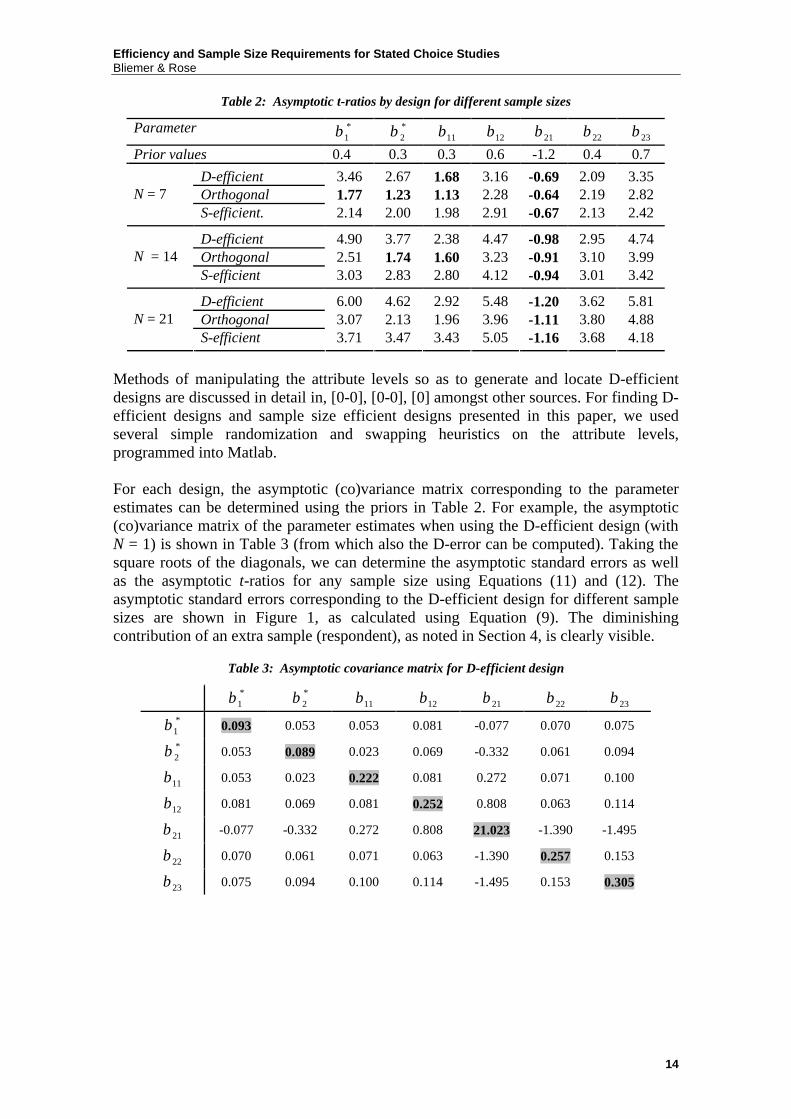
Table 2: Asymptotic t-ratios by design for different sample sizes

Parameter *1β *

2β 11β 12β 21β 22β 23β

Prior values 0.4 0.3 0.3 0.6 -1.2 0.4 0.7 D-efficient 3.46 2.67 1.68 3.16 -0.69 2.09 3.35 Orthogonal 1.77 1.23 1.13 2.28 -0.64 2.19 2.82 N = 7 S-efficient. 2.14 2.00 1.98 2.91 -0.67 2.13 2.42

D-efficient 4.90 3.77 2.38 4.47 -0.98 2.95 4.74 Orthogonal 2.51 1.74 1.60 3.23 -0.91 3.10 3.99 N = 14 S-efficient 3.03 2.83 2.80 4.12 -0.94 3.01 3.42

D-efficient 6.00 4.62 2.92 5.48 -1.20 3.62 5.81 Orthogonal 3.07 2.13 1.96 3.96 -1.11 3.80 4.88 N = 21 S-efficient 3.71 3.47 3.43 5.05 -1.16 3.68 4.18

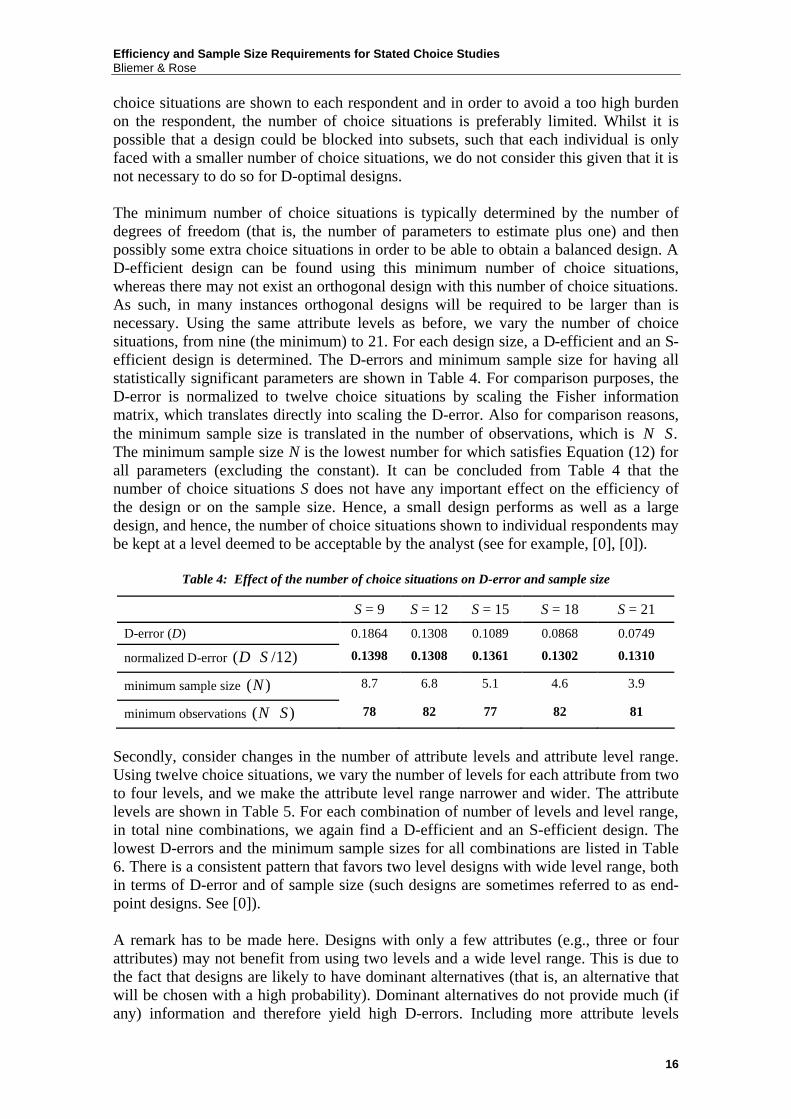
Methods of manipulating the attribute levels so as to generate and locate D-efficient designs are discussed in detail in, [0-0], [0-0], [0] amongst other sources. For finding D-efficient designs and sample size efficient designs presented in this paper, we used several simple randomization and swapping heuristics on the attribute levels, programmed into Matlab. For each design, the asymptotic (co)variance matrix corresponding to the parameter estimates can be determined using the priors in Table 2. For example, the asymptotic (co)variance matrix of the parameter estimates when using the D-efficient design (with N = 1) is shown in Table 3 (from which also the D-error can be computed). Taking the square roots of the diagonals, we can determine the asymptotic standard errors as well as the asymptotic t-ratios for any sample size using Equations (11) and (12). The asymptotic standard errors corresponding to the D-efficient design for different sample sizes are shown in Figure 1, as calculated using Equation (9). The diminishing contribution of an extra sample (respondent), as noted in Section 4, is clearly visible.

Table 3: Asymptotic covariance matrix for D-efficient design

*1β *

2β 11β 12β 21β 22β 23β *1β 0.093 0.053 0.053 0.081 -0.077 0.070 0.075 *2β 0.053 0.089 0.023 0.069 -0.332 0.061 0.094

11β 0.053 0.023 0.222 0.081 0.272 0.071 0.100

12β 0.081 0.069 0.081 0.252 0.808 0.063 0.114

21β -0.077 -0.332 0.272 0.808 21.023 -1.390 -1.495

22β 0.070 0.061 0.071 0.063 -1.390 0.257 0.153

23β 0.075 0.094 0.100 0.114 -1.495 0.153 0.305


15

0 2 4 6 8 10 12 14 16 18 200

0.1

0.2

0.3

0.4

0.5

*1

*2

11

12

22

23

β

βββββ

sample size

stan

dard

err

or

Figure 1: Standard errors when using the D-efficient design for different sample sizes Table 2 provides an insight into the design and statistical characteristics of the parameter estimates. In all three designs, it appears difficult to obtain a statistically significant parameter estimate for the constant ( 21β ). The asymptotic standard error of the parameter estimates can be positively influenced by making the attribute level range wider as will be demonstrated in Section 6.2. For the constant, this is not possible (i.e., the attribute level of the constant is fixed at one), however, as stated previously, the constant is typically ignored in SC experiments. Estimating parameter 11β seems to be

much more difficult than estimating parameters *1β and 23.β Using the S-efficient

design, a sample size of seven respondents (yielding 7 12 84× = choice observations) appears to be sufficient for obtaining significant parameter estimates for all of the attributes (except the constant), while larger sample sizes are necessary when using the other two designs. The orthogonal design performs poorly as a sample size of 14 respondents still yields several non-significant parameter estimates. It will need at least a sample size of 21 respondents to have all statistically significant parameter estimates (except the constant).

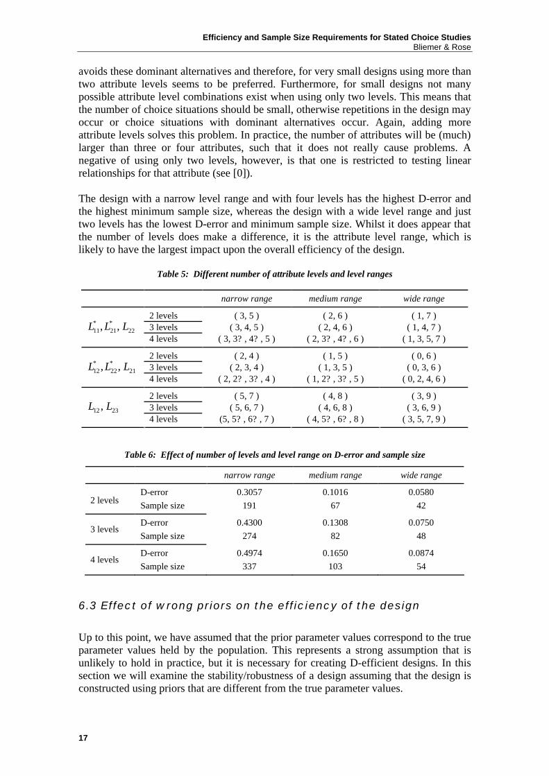
6.2 Effect of number of choice situations, attribute levels, and attribute level range In order to analyze the impact of different designs on the D-error (expressing the overall statistical efficiency of a design) and sample size efficiency, we will analyze the following effects: (i) effect of the number of choice situations S; (ii) effect of the number of attribute levels; and (iii) the effect of the attribute level range. First, let us change the number of choice situations S. In the analysis before we used twelve choice situations, which is essentially arbitrarily chosen (although for balancedness it should be a multiple of the number of attribute levels). Typically, all


16

choice situations are shown to each respondent and in order to avoid a too high burden on the respondent, the number of choice situations is preferably limited. Whilst it is possible that a design could be blocked into subsets, such that each individual is only faced with a smaller number of choice situations, we do not consider this given that it is not necessary to do so for D-optimal designs. The minimum number of choice situations is typically determined by the number of degrees of freedom (that is, the number of parameters to estimate plus one) and then possibly some extra choice situations in order to be able to obtain a balanced design. A D-efficient design can be found using this minimum number of choice situations, whereas there may not exist an orthogonal design with this number of choice situations. As such, in many instances orthogonal designs will be required to be larger than is necessary. Using the same attribute levels as before, we vary the number of choice situations, from nine (the minimum) to 21. For each design size, a D-efficient and an S-efficient design is determined. The D-errors and minimum sample size for having all statistically significant parameters are shown in Table 4. For comparison purposes, the D-error is normalized to twelve choice situations by scaling the Fisher information matrix, which translates directly into scaling the D-error. Also for comparison reasons, the minimum sample size is translated in the number of observations, which is .N S⋅ The minimum sample size N is the lowest number for which satisfies Equation (12) for all parameters (excluding the constant). It can be concluded from Table 4 that the number of choice situations S does not have any important effect on the efficiency of the design or on the sample size. Hence, a small design performs as well as a large design, and hence, the number of choice situations shown to individual respondents may be kept at a level deemed to be acceptable by the analyst (see for example, [0], [0]).

Table 4: Effect of the number of choice situations on D-error and sample size

S = 9 S = 12 S = 15 S = 18 S = 21

D-error (D) 0.1864 0.1308 0.1089 0.0868 0.0749

normalized D-error ( /12)D S⋅ 0.1398 0.1308 0.1361 0.1302 0.1310

minimum sample size ( )N 8.7 6.8 5.1 4.6 3.9

minimum observations ( )N S⋅ 78 82 77 82 81

Secondly, consider changes in the number of attribute levels and attribute level range. Using twelve choice situations, we vary the number of levels for each attribute from two to four levels, and we make the attribute level range narrower and wider. The attribute levels are shown in Table 5. For each combination of number of levels and level range, in total nine combinations, we again find a D-efficient and an S-efficient design. The lowest D-errors and the minimum sample sizes for all combinations are listed in Table 6. There is a consistent pattern that favors two level designs with wide level range, both in terms of D-error and of sample size (such designs are sometimes referred to as end-point designs. See [0]). A remark has to be made here. Designs with only a few attributes (e.g., three or four attributes) may not benefit from using two levels and a wide level range. This is due to the fact that designs are likely to have dominant alternatives (that is, an alternative that will be chosen with a high probability). Dominant alternatives do not provide much (if any) information and therefore yield high D-errors. Including more attribute levels


17

avoids these dominant alternatives and therefore, for very small designs using more than two attribute levels seems to be preferred. Furthermore, for small designs not many possible attribute level combinations exist when using only two levels. This means that the number of choice situations should be small, otherwise repetitions in the design may occur or choice situations with dominant alternatives occur. Again, adding more attribute levels solves this problem. In practice, the number of attributes will be (much) larger than three or four attributes, such that it does not really cause problems. A negative of using only two levels, however, is that one is restricted to testing linear relationships for that attribute (see [0]). The design with a narrow level range and with four levels has the highest D-error and the highest minimum sample size, whereas the design with a wide level range and just two levels has the lowest D-error and minimum sample size. Whilst it does appear that the number of levels does make a difference, it is the attribute level range, which is likely to have the largest impact upon the overall efficiency of the design.

Table 5: Different number of attribute levels and level ranges

narrow range medium range wide range

2 levels ( 3, 5 ) ( 2, 6 ) ( 1, 7 ) 3 levels ( 3, 4, 5 ) ( 2, 4, 6 ) ( 1, 4, 7 ) * *

11 21 22, ,L L L 4 levels ( 3, 3? , 4? , 5 ) ( 2, 3? , 4? , 6 ) ( 1, 3, 5, 7 )

2 levels ( 2, 4 ) ( 1, 5 ) ( 0, 6 ) 3 levels ( 2, 3, 4 ) ( 1, 3, 5 ) ( 0, 3, 6 ) * *

12 22 21, ,L L L 4 levels ( 2, 2? , 3? , 4 ) ( 1, 2? , 3? , 5 ) ( 0, 2, 4, 6 )

2 levels ( 5, 7 ) ( 4, 8 ) ( 3, 9 ) 3 levels ( 5, 6, 7 ) ( 4, 6, 8 ) ( 3, 6, 9 ) 12 23,L L 4 levels (5, 5? , 6? , 7 ) ( 4, 5? , 6? , 8 ) ( 3, 5, 7, 9 )

Table 6: Effect of number of levels and level range on D-error and sample size

narrow range medium range wide range

2 levels D-error Sample size

0.3057 191

0.1016 67

0.0580 42


0.4300 274

0.1308 82

0.0750 48


0.4974 337

0.1650 103

0.0874 54

6.3 Effect of wrong priors on the efficiency of the design Up to this point, we have assumed that the prior parameter values correspond to the true parameter values held by the population. This represents a strong assumption that is unlikely to hold in practice, but it is necessary for creating D-efficient designs. In this section we will examine the stability/robustness of a design assuming that the design is constructed using priors that are different from the true parameter values.


18

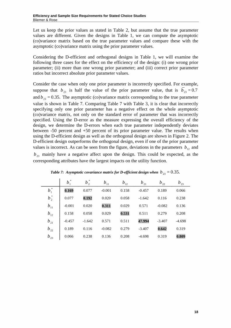
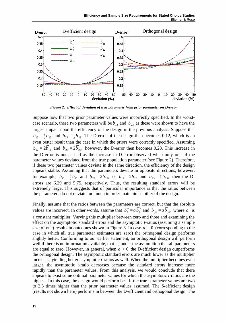
Let us keep the prior values as stated in Table 2, but assume that the true parameter values are different. Given the designs in Table 1, we can compute the asymptotic (co)variance matrix based on the true parameter values and compare these with the asymptotic (co)variance matrix using the prior parameter values. Considering the D-efficient and orthogonal designs in Table 1, we will examine the following three cases for the effect on the efficiency of the design: (i) one wrong prior parameter; (ii) more than one wrong prior parameter; and (iii) correct prior parameter ratios but incorrect absolute prior parameter values. Consider the case when only one prior parameter is incorrectly specified. For example, suppose that 23β is half the value of the prior parameter value, that is 23 0.7β = and 23 0.35.β = The asymptotic (co)variance matrix corresponding to the true parameter value is shown in Table 7. Comparing Table 7 with Table 3, it is clear that incorrectly specifying only one prior parameter has a negative effect on the whole asymptotic (co)variance matrix, not only on the standard error of parameter that was incorrectly specified. Using the D-error as the measure expressing the overall efficiency of the design, we determine the D-errors when each true parameter independently deviates between -50 percent and +50 percent of its prior parameter value. The results when using the D-efficient design as well as the orthogonal design are shown in Figure 2. The D-efficient design outperforms the orthogonal design, even if one of the prior parameter values is incorrect. As can be seen from the figure, deviations in the parameters 12β and

23β mainly have a negative affect upon the design. This could be expected, as the corresponding attributes have the largest impacts on the utility function.

Table 7: Asymptotic covariance matrix for D-efficient design when 23 0.35.β =

*1β *

2β 11β 12β 21β 22β 23β

*1β 0.169 0.077 -0.001 0.158 -0.457 0.189 0.066 *2β 0.077 0.192 0.020 0.058 -1.642 0.116 0.238

11β -0.001 0.020 0.311 0.029 0.571 -0.082 0.136

12β 0.158 0.058 0.029 0.531 0.511 0.279 0.208

21β -0.457 -1.642 0.571 0.511 47.994 -3.407 -4.698

22β 0.189 0.116 -0.082 0.279 -3.407 0.642 0.319

23β 0.066 0.238 0.136 0.208 -4.698 0.319 0.809


19

-50 -40 -30 -20 -10 0 10 20 30 40 50

0.15

0.2

0.25

0.3

0.35

0.4

0.45

0.5

-50 -40 -30 -20 -10 0 10 20 30 40 50

0.15

0.2

0.25

0.3

0.35

0.4

0.45

0.5

deviation (%) deviation (%)

D-error D-error

*1

*2

11

12

β

β

ββ

21

22

23

βββ

D-efficient design Orthogonal design

-50 -40 -30 -20 -10 0 10 20 30 40 50

0.15

0.2

0.25

0.3

0.35

0.4

0.45

0.5

-50 -40 -30 -20 -10 0 10 20 30 40 50

0.15

0.2

0.25

0.3

0.35

0.4

0.45

0.5


D-error D-error

*1

*2

11

12

β

β

ββ

21

22

23

βββ

-50 -40 -30 -20 -10 0 10 20 30 40 50

0.15

0.2

0.25

0.3

0.35

0.4

0.45

0.5

-50 -40 -30 -20 -10 0 10 20 30 40 50

0.15

0.2

0.25

0.3

0.35

0.4

0.45

0.5


D-error D-error

*1

*2

11

12

β

β

ββ

21

22

23

βββ


Figure 2: Effect of deviation of true parameter from prior parameter on D-error Suppose now that two prior parameter values were incorrectly specified. In the worst-case scenario, these two parameters will be 12β and 23β as these were shown to have the largest impact upon the efficiency of the design in the previous analysis. Suppose that

112 122β β= and 1

23 232 .β β= The D-error of the design then becomes 0.12, which is an even better result than the case in which the priors were correctly specified. Assuming

12 122β β= and 23 232 ,β β= however, the D-error then becomes 0.28. This increase in the D-error is not as bad as the increase in D-error observed when only one of the parameter values deviated from the true population parameter (see Figure 2). Therefore, if these two parameter values deviate in the same direction, the efficiency of the design appears stable. Assuming that the parameters deviate in opposite directions, however, for example, 1

12 122β β= and 23 232 ,β β= or 12 122β β= and 123 232 ,β β= then the D-

errors are 6.29 and 5.75, respectively. Thus, the resulting standard errors will be extremely large. This suggests that of particular importance is that the ratios between the parameters do not deviate too much in order maintain stability of the design. Finally, assume that the ratios between the parameters are correct, but that the absolute values are incorrect. In other words, assume that * *

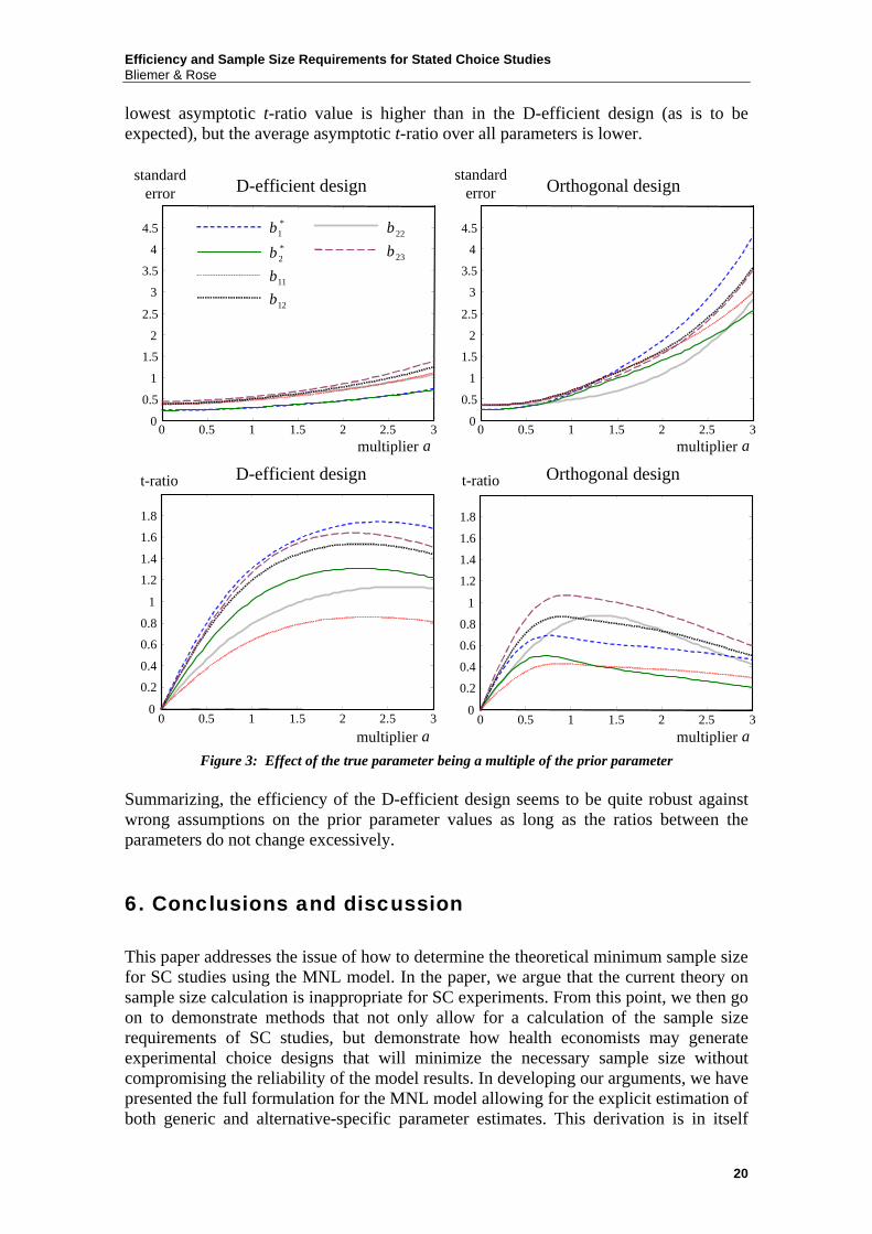
k kβ αβ= and ,jk jkβ αβ= where α is a constant multiplier. Varying this multiplier between zero and three and examining the effect on the asymptotic standard errors and the asymptotic t-ratios (assuming a sample size of one) results in outcomes shown in Figure 3. In case 0α = (corresponding to the case in which all true parameter estimates are zero) the orthogonal design performs slightly better. Conforming to our earlier statement, an orthogonal design will perform well if there is no information available, that is, under the assumption that all parameters are equal to zero. However, in general, when 0α > the D-efficient design outperforms the orthogonal design. The asymptotic standard errors are much lower as the multiplier increases, yielding better asymptotic t-ratios as well. When the multiplier becomes even larger, the asymptotic t-ratio decreases because the standard errors increase more rapidly than the parameter values. From this analysis, we would conclude that there appears to exist some optimal parameter values for which the asymptotic t-ratios are the highest. In this case, the design would perform best if the true parameter values are two to 2.5 times higher than the prior parameter values assumed. The S-efficient design (results not shown here) performs in between the D-efficient and orthogonal design. The


20

lowest asymptotic t-ratio value is higher than in the D-efficient design (as is to be expected), but the average asymptotic t-ratio over all parameters is lower.

0 0.5 1 1.5 2 2.5 30

0.5

1

1.5

2

2.5

3

3.5

4

4.5

0 0.5 1 1.5 2 2.5 30

0.5

1

1.5

2

2.5

3

3.5

4

4.5

0 0.5 1 1.5 2 2.5 30

0.2

0.4

0.6

0.8

1

1.2

1.4

1.6

1.8

0 0.5 1 1.5 2 2.5 30

0.2

0.4

0.6

0.8

1

1.2

1.4

1.6

1.8

multiplier α multiplier α

multiplier αmultiplier α

standarderror

standarderror

t-ratio t-ratio



*1

*2

11

12

β

β

ββ

22

23

ββ

Figure 3: Effect of the true parameter being a multiple of the prior parameter

Summarizing, the efficiency of the D-efficient design seems to be quite robust against wrong assumptions on the prior parameter values as long as the ratios between the parameters do not change excessively.

6. Conclusions and discussion This paper addresses the issue of how to determine the theoretical minimum sample size for SC studies using the MNL model. In the paper, we argue that the current theory on sample size calculation is inappropriate for SC experiments. From this point, we then go on to demonstrate methods that not only allow for a calculation of the sample size requirements of SC studies, but demonstrate how health economists may generate experimental choice designs that will minimize the necessary sample size without compromising the reliability of the model results. In developing our arguments, we have presented the full formulation for the MNL model allowing for the explicit estimation of both generic and alternative-specific parameter estimates. This derivation is in itself


21

innovative as it differs from previous research, which cite as the basis of their work, McFadden [0]. As shown by Bliemer and Rose and Rose and Bliemer [0-0], the original work of McFadden was limited to the specific case of the MNL model with generic parameter estimates only. Nevertheless, despite this limitation, some authors have incorrectly used the MNL specification provided by McFadden to optimize designs with alternative specific parameter estimates (see for example [0]). As such, as well as addressing the issues of sample size, this paper also addresses the issue recently raised by Viney et al. [0] as to the generation of efficient designs for problems requiring the estimation of alternative-specific parameter estimates. Viney et al. [0] state in their concluding remarks “it is clear that for health care, the choice contexts are often complex, and the relevant alternatives may not be readily captured in experiments with relatively small numbers of attributes, or in experiments with generic attributes, for which optimal design results are known. There are challenges in determining optimal experimental designs for choice experiments where attributes are labelled and both attributes and levels vary across alternatives, or where there are both context and choice variables that are relevant to the choice.” (p361). The results from our analysis show that D-efficient and S-efficient designs outperform orthogonal designs in terms of the reliability of the parameter estimates as well as in terms of the need for lower sample sizes, provided that there exists some prior information which may be used to help generate the design. Given even limited information (even if only on the sign of the parameter estimates), it is possible to generate statistically more efficient designs that require significantly smaller sample sizes. Although there exists the need to conduct further research on a wider number of designs, from the results shown herein, we would suggest that orthogonal designs should only ever be used when there exists no information with regards to the likely parameter estimates for the design to be generated. However, even in such cases where no information is available, we have demonstrated that D-efficient and S-efficient designs may possibly outperform orthogonal designs, even if the priors used in their construction are incorrectly specified. The methods we have outlined within this paper allow for a sensitivity analysis (without having to rely on Monte Carlo methods) with regards to the priors specified in the generation of optimal designs. This sensitivity analysis provides a means to determine whether one should rely on an orthogonal design, or assume some information about the priors, even if such information is likely to be incorrect. In support of this supposition, it would appear that an (D- or S-) efficient design is stable as long as the parameter ratios are more or less correct. In this paper, we have also examined the role various design dimensions play in producing optimal SC designs. From our analysis, we would conclude that the number of choice situations provided to respondents does not impact (at least statistically; behaviorally this may not be the case) the reliability of the parameter estimates. Importantly, the attribute level range employed in the study does appear to have a significant impact on the ability to locate designs with greater levels of statistical efficiency. Our results suggest that the wider the range, the easier it is to produce designs with greater reliability in the parameter estimates. This should be tempered, however, with other considerations, particularly related to the sampled respondents. For behavioral reasons, the attribute levels should be designed such that respondents can reasonably answer the survey in a serious manner. Our analysis also suggests that fewer


22

attribute levels are better than many. Indeed, our results have shown that end point designs (designs using only the two widest attribute levels) will be much more efficient than designs with attribute levels positioned within the attribute level width. Again, this finding should be considered with some caution. End point designs allow only for the estimation of linear marginal effects. Thus, such designs are appropriate only when the analyst is willing to make the assumption that the marginal utilities for an attribute are linear between the two design points (i.e., attribute levels) used. This may prove too strong an assumption in many instances, particularly when an attribute is categorical in nature.

References Louviere, J.J. and Woodworth, G. Design and analysis of simulated consumer choice or allocation experiments: an approach based on aggregate data, J Marketing Research; 1983, 20, 350-367.

Louviere, J.J. and Hensher, D.A. Using Discrete Choice Models with Experimental Design Data to Forecast Consumer Demand for a Unique Cultural Event, J Consumer Research;1983, 10 (December), 348-361.

Telser H. and Zweifel P. Measuring willingness-to-pay for risk reduction: an application of conjoint analysis, Health Economics 2002; 11, 129-139.

Hall, J. Kenny P., King M., Louviere J., Viney R. and Yeoh A. Using stated preference discrete choice modelling to evaluate the introduction of varicella vaccination, Health Economics 2002; 11: 457–465.

Mark, T.L. and Swait, J. Using stated preference and revealed preference modeling to evaluate prescribing decisions, Health Economics 2004; 13: 563–573.

Mooney JS, Ryan M, Bruggemann K, Alexander K. The use of conjoint analysis to elicit community preferences in public health research: a case study of hospital services in South Australia. Aust NZ J Public Health 2000; 24(1): 64–70.

Ryan M, Scott DA, Reeves C et al. Eliciting public preferences for health care: a systematic review of techniques. Health Technol Assess 2001; 5(5).

Cookson, R. Willingness to pay methods in health care: a sceptical view, Health Economics 2003; 12: 891–894.

Lloyd, A.J. Threats to the estimation of benefit: are preference elicitation methods accurate? Health Economics 2003; 12: 393–402.

Skjoldborg, U.S. and Gyrd-Hansen, D. Conjoint analysis. The cost variable: an Achilles’ heel? Health Economics 2003; 12: 479-491.

Carson, R., Louviere, J.J., Anderson, D., Arabie, P., Bunch, D., Hensher, D.A, Johnson, R., Kuhfeld, W., Steinberg, D., Swait, J., Timmermans, H., and Wiley, J. Experimental Analysis of Choice, Marketing Letters 1994, 5 (October), 351-367.

Cooke, A.D. and Mellers, B.A. Attribute Range and Response Range: Limits of Compatibility in Multiattribute Judgment, Organizational Behavior and Human Decision Processes 1995; 63(2), 187-194.


23

Brazell, J.D. and Louviere, J.J. Length effects in conjoint choice experiments and surveys: an explanation based on cumulative cognitive burden. Department of Marketing 1998, The University of Sydney, July.

Pullman, M.E., Dodson, K.J., and Moore, W.L., A Comparison of Conjoint Methods When There Are Many Attributes, Marketing Letters 1999; 10(2), 1-14.

Ohler, T., Li. A., Louviere, J.J., and Swait, J. Attribute range effects in binary response tasks Marketing Letters 2000; 11, 3, 249-260.

DeShazo, J.R. and Fermo G. Designing choice sets for stated preference methods: the effects of complexity on choice consistency, J Environmental Economics and Management 2002; 44, 1, 123-143.

Verlegh, P.W., Schifferstein, H.N., and Wittink D.R. Range and Number-of-Levels Effects in Derived and Stated Measures of Attribute Importance, Marketing Letters 2002; 13, 1, 41-52.

Arentze, T., Borgers, A., Timmermans, H., and DelMistro, R. Transport stated choice responses: effects of task complexity, presentation format and literacy, Transportation Research Part E 2003; 39, 229–244.

Louviere, J.J., Timmermans, H.J.P. Hierarchical information integration applied to residential choice behaviour, Geographical Analysis, 1990; 22, 127–145.

Oppewal, H., Louviere, J.J., Timmermans, H.J.P. Modeling hierarchical information integration processes with integrated conjoint choice experiments. J Marketing Research 1994; 31, 92–105.

Maddala T., Phillip K.A. and Johnson, F.R. An experiment on simplifying conjoint analysis designs for measuring preferences, Health Economics 2003; 12: 1035-1047.

Chapman, R.G. and Staelin, R. Exploiting Rank Ordered Choice Set Data within the Stochastic Utility Model, Journal of Marketing Research 1982; 19, 288-301.

Bunch, D.S., Louviere, J.J., and Anderson D. A Comparison of Experimental Design Strategies for Choice-Based Conjoint Analysis with Generic-Attribute Multinomial Logit Models, Working Paper 1996; Graduate School of Management, University of California, Davis.

Huber, J. and Zwerina, K. The Importance of Utility Balance in Efficient Choice Designs. Journal of Marketing Research 1996; 33, 307-317.

Carlsson, F. and Peter Martinsson, P. Design techniques for stated preference methods in health economics, Health Economics 2002; 12, 281-294.

Manski, C.F. and McFadden, D. Alternative Estimators and Sample Designs for Discrete Choice Analysis. In C.F. Manski and D. McFadden (eds.), Structural Analysis of Discrete Data with Econometric Applications 1981; 2-50, MIT Press: Cambridge, MA.

Ben-Akiva, M. and Lerman, S.R. Discrete Choice Analysis: Theory and Application to Travel Demand 1985; MIT Press.

Hensher, D.A., Rose, J.M. and Greene, W.H. Applied Choice Analysis: A Primer, Cambridge University Press, 2005; Cambridge.

Louviere, J.J. and Hensher, D.A. and Swait, J.D. Stated Choice Methods: Analysis and Application 2000; Cambridge University Press, Cambridge.


24

McFadden, D. Conditional Logit Analysis of Qualitative Choice Behavior. In Frontiers in Econometrics 1974, Zarembka (ed.), Academic Press, New York, 105-142.

Sandor, Z. and Wedel, M. Designing Conjoint Choice Experiments Using Managers’ Prior Beliefs, J Marketing Research 2001; 38 (November), 430-444.

Kanninen, B.J. Optimal Design for Multinomial Choice Experiments, J Marketing Research 2002; 39 (May), 214-217.

Bliemer, M.C.J and Rose, J.M. Efficient Designs for Alternative Specific Choice Experiments, Working Paper 2005; University of Sydney, February.

Rose, J.M. and Bliemer, M.C.J Constructing Efficient Choice Experiments with Alternative Specific and Generic Parameter Estimates, Working Paper 2005; University of Sydney, April.

Kuhfeld, W.F., Tobias, R.D., and Garratt, M. Efficient Experimental Design with Marketing Research Applications, J Marketing Research 1994, 21 (November), 545-557.

Viney, R. Savage, E. and Louviere, J. Empirical investigation of experimental design properties of discrete choice experiments in health 2005; 14, 349-362.

institute of transport and logistics studies - the university of sydney...

Documents