institute of computer science academy of sciences of …handbook.pdf · institute of computer...

Institute of Computer ScienceAcademy of Sciences of the Czech Republic

A Handbook of Results on IntervalLinear ProblemsDedicated in memoriam to my parents

Mrs. Nina Rohnova and Mr. Robert Rohn

Jirı Rohnhttp://uivtx.cs.cas.cz/~rohn

Technical report No. V-1163

07.04.2005 / 23.09.2012

Pod Vodarenskou vezı 2, 182 07 Prague 8, phone: +420 266 051 111, fax: +420 286 585 789,e-mail:[email protected]

http://uivtx.cs.cas.cz/~rohn�

Institute of Computer ScienceAcademy of Sciences of the Czech Republic

A Handbook of Results on IntervalLinear ProblemsDedicated in memoriam to my parents

Mrs. Nina Rohnova and Mr. Robert Rohn

Jirı Rohnhttp://uivtx.cs.cas.cz/~rohn

Technical report No. V-1163

07.04.2005 / 23.09.2012

Abstract:

This text surveys important results on interval matrices, interval linear equations (both squareand rectangular), and interval linear programming (without proofs). It is based on a “one-topic-one-page” approach, in which each topic is allotted the space of one page only, and containsMATLAB-like descriptions of 15 basic algorithms. The bibliography contains direct links to manypapers quoted. Verification versions of some of the algorithms presented in the text can be foundin the VERSOFT software package. The Handbook was finalized on 07.04.2005 and was left asan internet text only; here it is published in its original 2005 form as a technical report. Duringthe years 2005-2012 many of the results have been improved; they can be found at author’s webpage http://uivtx.cs.cas.cz/~rohn/publist/000home.htm.

1

Keywords:Interval linear problems, auxiliary results, interval matrices, systems of interval linear equations(square case), systems of interval linear equations and inequalities (rectangular case), intervallinear programming, algorithms, and many others.

1Above: logo of interval computations and related areas (depiction of the solution set of the system[2, 4]x1 + [−2, 1]x2 = [−2, 2], [−1, 2]x1 + [2, 4]x2 = [−2, 2] (Barth and Nuding [6])).

http://uivtx.cs.cas.cz/~rohn�

http://uivtx.cs.cas.cz/~rohn/publist/000home.htm�

Motto

Was sich uberhaupt sagen laßt, laßt sich klar sagen;und wovon man nicht reden kann, daruber muß man schweigen.

L. Wittgenstein, Tractatus logico-philosophicus,Routledge & Kegan Paul Ltd., London 1922

Contents

Preface 5

1 Notations 7

1.1 Basic notations . . . . . . . . . . . . . . . . . . . . . . . . . . . . . . . . . . . 8

1.1.1 Linear algebraic notations . . . . . . . . . . . . . . . . . . . . . . . . . 8

1.1.2 Specific notations . . . . . . . . . . . . . . . . . . . . . . . . . . . . . . 8

1.2 Summary: Linear algebraic notations . . . . . . . . . . . . . . . . . . . . . . . 9

1.3 Summary: Specific notations . . . . . . . . . . . . . . . . . . . . . . . . . . . 10

2 Auxiliary results 11

2.1 The set Yn . . . . . . . . . . . . . . . . . . . . . . . . . . . . . . . . . . . . . . 12

2.2 The norm ‖A‖∞,1 . . . . . . . . . . . . . . . . . . . . . . . . . . . . . . . . . . 13

2.3 The equation Ax + B|x| = b and the sign accord algorithm . . . . . . . . . . 14

3 Interval matrices 15

3.1 Interval matrices: definition and basic notations . . . . . . . . . . . . . . . . . 16

3.2 Regularity . . . . . . . . . . . . . . . . . . . . . . . . . . . . . . . . . . . . . . 17

3.3 Finding a singular matrix . . . . . . . . . . . . . . . . . . . . . . . . . . . . . 18

3.4 Qz matrices . . . . . . . . . . . . . . . . . . . . . . . . . . . . . . . . . . . . . 19

3.5 Inverse interval matrix . . . . . . . . . . . . . . . . . . . . . . . . . . . . . . . 20

3.6 Enclosure of the inverse interval matrix . . . . . . . . . . . . . . . . . . . . . 21

3.7 Inverse stability . . . . . . . . . . . . . . . . . . . . . . . . . . . . . . . . . . . 22

3.8 Inverse sign pattern . . . . . . . . . . . . . . . . . . . . . . . . . . . . . . . . 23

3.9 Inverse nonnegativity . . . . . . . . . . . . . . . . . . . . . . . . . . . . . . . . 24

3.10 Radius of regularity . . . . . . . . . . . . . . . . . . . . . . . . . . . . . . . . 25

3.11 Real eigenvalues . . . . . . . . . . . . . . . . . . . . . . . . . . . . . . . . . . 26

3.12 Real eigenvectors . . . . . . . . . . . . . . . . . . . . . . . . . . . . . . . . . . 27

3.13 Real eigenpairs . . . . . . . . . . . . . . . . . . . . . . . . . . . . . . . . . . . 28

1

3.14 Eigenvalues of symmetric matrices . . . . . . . . . . . . . . . . . . . . . . . . 29

3.15 Positive semidefiniteness . . . . . . . . . . . . . . . . . . . . . . . . . . . . . . 30

3.16 Positive definiteness . . . . . . . . . . . . . . . . . . . . . . . . . . . . . . . . 31

3.17 Hurwitz stability . . . . . . . . . . . . . . . . . . . . . . . . . . . . . . . . . . 32

3.18 Schur stability . . . . . . . . . . . . . . . . . . . . . . . . . . . . . . . . . . . 33

3.19 Full column rank . . . . . . . . . . . . . . . . . . . . . . . . . . . . . . . . . . 34

4 Interval linear equations (square case) 35

4.1 Interval vectors: definition and basic notations . . . . . . . . . . . . . . . . . 36

4.2 The solution set . . . . . . . . . . . . . . . . . . . . . . . . . . . . . . . . . . . 37

4.3 The hull . . . . . . . . . . . . . . . . . . . . . . . . . . . . . . . . . . . . . . . 38

4.4 The solution set lying in a single orthant . . . . . . . . . . . . . . . . . . . . . 39

4.5 Enclosure of the solution set . . . . . . . . . . . . . . . . . . . . . . . . . . . . 40

4.6 Overestimation of the HBR enclosure . . . . . . . . . . . . . . . . . . . . . . . 41

5 Interval linear equations and inequalities (rectangular case) 42

5.1 (Z, z)-solutions . . . . . . . . . . . . . . . . . . . . . . . . . . . . . . . . . . . 43

5.2 Tolerance solutions . . . . . . . . . . . . . . . . . . . . . . . . . . . . . . . . . 44

5.3 Control solutions . . . . . . . . . . . . . . . . . . . . . . . . . . . . . . . . . . 45

5.4 Strong solvability of equations . . . . . . . . . . . . . . . . . . . . . . . . . . . 46

5.5 Strong solvability of inequalities . . . . . . . . . . . . . . . . . . . . . . . . . . 47

6 Interval linear programming 48

6.1 Reminder: optimal value of a linear program . . . . . . . . . . . . . . . . . . 49

6.2 Range of the optimal value . . . . . . . . . . . . . . . . . . . . . . . . . . . . 50

7 Algorithms 51

7.1 An algorithm for generating the set Yn . . . . . . . . . . . . . . . . . . . . . . 52

7.2 An algorithm for computing the norm ‖A‖∞,1 . . . . . . . . . . . . . . . . . . 53

7.3 The sign accord algorithm . . . . . . . . . . . . . . . . . . . . . . . . . . . . . 54

7.4 An algorithm for checking regularity . . . . . . . . . . . . . . . . . . . . . . . 55

7.5 An algorithm for finding a singular matrix . . . . . . . . . . . . . . . . . . . . 56

7.6 An algorithm for computing Qz . . . . . . . . . . . . . . . . . . . . . . . . . . 57

7.7 An algorithm for computing the inverse . . . . . . . . . . . . . . . . . . . . . 58

7.8 An algorithm for checking positive definiteness . . . . . . . . . . . . . . . . . 59

7.9 An algorithm for checking Hurwitz stability . . . . . . . . . . . . . . . . . . . 60

7.10 An algorithm for checking Schur stability . . . . . . . . . . . . . . . . . . . . 61

2

7.11 An algorithm for computing the hull . . . . . . . . . . . . . . . . . . . . . . . 62

7.12 The Hansen-Bliek-Rohn enclosure algorithm . . . . . . . . . . . . . . . . . . . 63

7.13 An algorithm for checking strong solvability of equations . . . . . . . . . . . . 64

7.14 An algorithm for checking strong solvability of inequalities . . . . . . . . . . . 65

7.15 An algorithm for computing the range of the optimal value . . . . . . . . . . 66

Bibliography 67

3

Preface

Aim. It has been the aim of this text to present a selection of important results on intervallinear problems in a unified and concise way.

Philosophy. The philosophy behind the text is the “one-topic-one-page” approach, in whicheach topic is allotted the space of one page only.

Layout. There are basically two types of problems handled in interval analysis: decisionproblems (as checking whether an interval matrix is regular), and computational problems(as computation of the inverse of a regular interval matrix). For decision problems I wasusing the following page layout:

Definition. (basic notion of the page)

Problem. (problem formulation)

Necessary and sufficient condition.

Complexity.

Sufficient condition. (if the problem is NP-hard)

Algorithm. (reference to Chapter 7, or to the above sufficient condition)

Comment. (if necessary)

Operation. (the way the algorithm is operating)

Special features. (explanations, connections or related results of particular interest)

References. (sources of given or related results; without names)

and for the computational problems a similar layout

Definition.

Problem.

Formula(e). (formula(e) used in the algorithm)

Complexity.

Algorithm.

Comment.

Operation.

Special features.

References.

Sometimes some of the headings are missing. Occasionally, when necessary, I also added

5

another headings, as Intro, Fact, Idea, Formulae for enclosures, Apology2, etc.

Algorithms. It has been my second goal to present not-a-priori-exponential algorithms forsolving NP-hard problems. They are those forming the branch starting with signaccord inthe scheme on p. 51.

Algorithm form. All the algorithms are gathered in Chapter 7. They are described in theform of MATLAB-like functions, but with formulae written in the usual mathematical way.In particular, the output variable flag always gives a verbal description of the output.

Hyperlinks. The source text contains hyperlinks that make it easy to flip through it simplyby clicking on links colored in magenta, or, in the Contents, in blue. In particular, each itemin the bibliography is appended with numbers (in magenta) of the pages where it is referencedfrom. (This feature also allows you to verify that all the bibliographical items have beenreferenced.) My own papers listed can be downloaded directly by clicking on the respectiveURLs in the bibliography.3

Prague, Easter 2005 Jiri Rohn([email protected])

2On p. 40.3Unfortunately, this works only in the dvi file, not in the pdf file.

6

Chapter 1

Notations

Subject. Notations used are introduced and summarized in this chapter.

7

1.1 Basic notations

1.1.1 Linear algebraic notations

Notation for matrices. The ith row of a matrix A is denoted by Ai•, the jth columnby A•j . For two matrices A,B of the same size, inequalities like A ≤ B or A < B areunderstood componentwise. A is called nonnegative if 0 ≤ A and symmetric if AT = A; AT

is the transpose of A. A ◦ B denotes the Hadamard (entrywise) product of A,B ∈ Rm×n,i.e., (A ◦ B)ij = AijBij for each i, j. The absolute value of a matrix A = (aij) is defined by|A| = (|aij |). Maximum (or minimum) of two matrices A, B is taken componentwise, i.e.,(max{A,B})ij = max{Aij , Bij} for each i, j.

Properties. The following properties are valid whenever the respective operations andinequalities are defined: (i) A ≤ B and 0 ≤ C imply AC ≤ BC, (ii) A ≤ |A|, (iii) |A| ≤ B ifand only if −B ≤ A ≤ B, (iv) |A+B| ≤ |A|+ |B|, (v) if A◦B ≥ 0, then |A+B| = |A|+ |B|,(vi) if |A−B| < |B|, then A ◦B > 0, (vii) ||A| − |B|| ≤ |A−B|, (viii) |AB| ≤ |A||B|.Notation for vectors. The same notations and results also apply to vectors which arealways considered one-column matrices. Hence, for a = (ai) and b = (bi), aT b =

∑i aibi is

the scalar product whereas abT is the matrix (aibj).

Notation. I denotes the unit matrix, ej is the jth column of I, e = (1, . . . , 1)T is the vectorof all ones and E = eeT ∈ Rm×n is the matrix of all ones (in these cases we do not designateexplicitly the dimension which can always be inferred from the context).

1.1.2 Specific notations

Notation specific for this text. Throughout the text, important role is played by the setYm of all ±1 vectors in Rm, i.e., Ym = {y ∈ Rm ; |y| = e}. Obviously, the cardinality of Ym

is 2m. For each x ∈ Rm we define its sign vector sgnx by

(sgn x)i ={

1 if xi ≥ 0,−1 if xi < 0

(i = 1, . . . ,m),

so that sgnx ∈ Ym. For a given vector y ∈ Rm we denote

Ty =

y1 0 . . . 00 y2 . . . 0...

.... . .

...0 0 . . . ym

. (1.1)

With a few exceptions we use the notation Ty for vectors y ∈ Ym only, in which case wehave T−y = −Ty, T−1

y = Ty and |Ty| = I. For each x ∈ Rm we can write |x| = Tzx, wherez = sgnx; in the proofs1 this trick is often used to remove the absolute value of a vector.Notice that Tzx = (zixi)m

i=1 = z ◦ x.

All notations are summed up on pp. 9-10.

1Omitted here.

8

1.2 Summary: Linear algebraic notations

A matrixAi• the ith row of AA•j the jth column of AA−1 inverse matrixA+ the Moore-Penrose inverse of AAT transpose of A‖A‖∞,1 = max‖x‖∞=1 ‖Ax‖1

A ≤ B Aij ≤ Bij for each i, jA < B Aij < Bij for each i, jA ≥ B ⇔ B ≤ AA > B ⇔ B < AA ◦B = (aijbij) for A = (aij), B = (bij) (Hadamard product)a column vectoraT b =

∑i aibi (scalar product)

abT outer product ((abT )ij = aibj for each i, j)Conv X the convex hull of XdetA determinant of AE = eeT ∈ Rm×n (the matrix of all ones)e = (1, 1, . . . , 1)T

ej the jth column of the unit matrix II unit (or identity) matrixλi(A) the ith eigenvalue of a symmetric A (λ1(A) ≥ . . . ≥ λn(A))max{A,B} componentwise maximum of matrices (vectors)min{A,B} componentwise minimum of matrices (vectors)R the set of real numbersRm×n the set of m× n real matricesRn real vector space%(A) spectral radius of A

9

1.3 Summary: Specific notations

Notations marked in red are important and occur frequently.

A interval matrix|A| absolute value of a matrix (|A| = (|aij |) for A = (aij))A lower bound of an interval matrix A = [A, A]A upper bound of an interval matrix A = [A,A]Ac midpoint matrix of an interval matrix A = [Ac −∆, Ac + ∆]As = [(A + AT )/2, (A + A

T )/2] for A = [A, A] (symmetrization)Ayz = Ac − Ty∆Tz

A−yz = A−y,za0 = 0 for a = 0, = ∞ for a > 0 (case a < 0 does not occur)b interval vectorb lower bound of an interval vector b = [b, b]b upper bound of an interval vector b = [b, b]bc midpoint vector of an interval vector b = [bc − δ, bc + δ]by = bc + Ty∆δ radius vector of an interval vector b = [bc − δ, bc + δ]∆ radius matrix of an interval matrix A = [Ac −∆, Ac + ∆]f(A, b, c) optimal value of a linear programming problemf(A,b, c) lower bound of the range of the optimal value of an

interval linear programming problemf(A,b, c) upper bound of the range of the optimal value of an

interval linear programming problem%0(A) real spectral radius of A (maximum of moduli of real eigenvalues)

= 0 if no real eigenvalue existsRn

z = {x ∈ Rn ; Tzx ≥ 0} (z-orthant, z ∈ Yn)sgnx sign vector of a vector x ((sgnx)i = 1 if xi ≥ 0, (sgnx)i = −1 otherwise)Ty the diagonal matrix with diagonal vector yX the solution set of Ax = b|x| absolute value of a vector (|x| = (|xi|) for x = (xi))[x, x] the interval hull of the solution set X[x, x] enclosure of X (in particular, that by Hansen-Bliek-Rohn)Ym the set of all ±1-vectors in Rm

10

Chapter 2

Auxiliary results

Recommendation. Please, read the Preface (pp. 5-6) first.

Subject. Three auxiliary results (of noninterval character) are presented in this chapter.

11

2.1 The set Yn

Definition. Yn is the set of all ±1-vectors in Rn (there are 2n of them).

Problem. Generate Yn vector by vector so that each two successive vectors differ in exactlyone entry.

Algorithm. See p. 52.

Comment. In the algorithm description, y is the generated vector and z is an auxiliary(0, 1)-vector used for determining the index k for which yk should be changed to −yk.

Operation. For each n ≥ 1 the algorithm at the output yields the set Y = Yn.

Special features. This algorithm is employed as a subroutine in exhaustive algorithmsthat require to perform some operation for all y ∈ Yn (see the scheme on p. 51). The set Yn

itself is not constructed, the operation is applied to successively generated vectors.

References. [108].

12

2.2 The norm ‖A‖∞,1

Definition. For A ∈ Rm×n we define (see e.g. [35])

‖A‖∞,1 = max‖x‖∞=1

‖Ax‖1.

Problem. Compute ‖A‖∞,1 for a given A.

Formula. For each A ∈ Rm×n we have

‖A‖∞,1 = maxy∈Yn

‖Ay‖1.

Complexity. Computing ‖A‖∞,1 is NP-hard. Even more, checking whether ‖A‖∞,1 ≥ 1 isNP-complete.


Comment. This algorithm uses implicitly the algorithm ynset for generating the set Yn (p.52). This simplifies computation of the new Ay′ from the old Ay. Also, since ‖A(−y)‖1 =‖Ay‖1, only y’s with yn = 1 are considered.

Operation. The algorithm computes ‖A‖∞,1 in a number of steps exponential in n.

Special features. When studying complexity of interval linear problems, we often encounterthis norm (see the survey [105]). Since its computation is NP-hard, the norm forms one oftwo main tools for establishing NP-hardness of interval linear problems (the second such atool is a related problem whether −e ≤ Ax ≤ e, ‖x‖1 ≥ 1 has a solution, see [108]).

References. [107], [105], [108], [35], [25].

13

2.3 The equation Ax + B|x| = b and the sign accord algorithm

Problem. Given A,B ∈ Rn×n and b ∈ Rn, find a solution to the nonlinear equation

Ax + B|x| = b. (2.1)

Idea. If we knew the sign vector z = sgnx of the solution x of (2.1), we could rewrite (2.1)as (A + BTz)x = b and solve it for x as x = (A + BTz)−1b. However, we know neither x,nor z; but we do know that they should satisfy Tzx = |x| ≥ 0, i.e., zjxj ≥ 0 for each j (asituation we call a sign accord of z and x). In its kernel form the sign accord algorithmcomputes the z’s and x’s repeatedly until a sign accord occurs. A combinatorial argument

z = sgn (A−1b);x = (A + BTz)−1b;while zjxj < 0 for some j

k = min{j ; zjxj < 0};zk = −zk;x = (A + BTz)−1b;

end

Figure 2.1: The kernel of the sign accord algorithm (p. 54).

is used to prove that in case of regularity of [A − |B|, A + |B| ], a sign accord is achievedwithin a prespecified number of steps, so that crossing this number indicates singularity of[A− |B|, A + |B| ] (see p. 17 for regularity and singularity).

Complexity. The problem of checking whether (2.1) has a solution is NP-complete.


Comment. The matrix C in the algorithm description is used for updating x according tothe Sherman-Morrison formula.

Operation. For each A,B ∈ Rn×n and each b ∈ Rn, the sign accord algorithm (p. 54) ina finite number of steps either finds a solution of the equation (2.1), or states singularityof the interval matrix [A − |B|, A + |B| ] (and, in certain cases, finds a singular matrixAs ∈ [A− |B|, A + |B| ]).Comment. If [A−|B|, A+ |B| ] is regular, then the algorithm finds a solution of (2.1) which,moreover, is unique. In case of singularity the algorithm may state singularity without havingfound a singular matrix, but such cases are rather rare; in most cases it finds a singular matrixas well.

Special features. The sign accord algorithm is the fundamental building block for con-struction of other algorithms presented in Chapter 7. (See the scheme on p. 51.)

References. [92].

14

Chapter 3

Interval matrices

Subject. In this chapter we consider various properties of square n × n interval matrices.Rectangular interval matrices are handled only in the last Section 3.19.

15

3.1 Interval matrices: definition and basic notations

Definition. If A, A are two matrices in Rm×n, A ≤ A, then the set of matrices

A = [A, A] = {A ; A ≤ A ≤ A}is called an interval matrix, and the matrices A, A are called its bounds.

Comment. Hence, if A = (aij) and A = (aij), then A is the set of all matrices A = (aij)satisfying

aij ≤ aij ≤ aij (3.1)

for i = 1, . . . ,m, j = 1, . . . , n. It is worth noting that each coefficient may attain any valuein its interval (3.1) independently of the values taken on by other coefficients. Notice thatinterval matrices are typeset in boldface letters.

Notation. In many cases it is more advantageous to express the data in terms of the centermatrix

Ac = 12(A + A) (3.2)

and of the radius matrix∆ = 1

2(A−A), (3.3)

which is always nonnegative.

Comment. From (3.2), (3.3) we easily obtain that

A = Ac −∆,

A = Ac + ∆,

so that A can be given either as [A, A], or as [Ac − ∆, Ac + ∆]. In the sequel we employboth forms and we switch freely between them according to which one is more useful in thecurrent context.

Matrices Ayz (important). Given an m × n interval matrix A = [Ac − ∆, Ac + ∆], wedefine matrices

Ayz = Ac − Ty∆Tz

for each y ∈ Ym and z ∈ Yn (Ty is given by (1.1)).

Explanation. The definition implies that

(Ayz)ij = (Ac)ij − yi∆ijzj ={

aij if yizj = −1,aij if yizj = 1

(i = 1, . . . , m, j = 1, . . . , n), so that Ayz ∈ A for each y ∈ Ym, z ∈ Yn.

Special features. This finite set of matrices from A (of cardinality at most 2m+n−1 becauseAyz = A−y,−z for each y ∈ Ym, z ∈ Yn; the bound is attained if ∆ > 0) plays an importantrole because it turns out that many problems with interval-valued data can be characterizedin terms of these matrices, thereby obtaining finite characterizations of problems involvinginfinitely many sets of data.

Special cases. We write A−yz instead of A−y,z. In particular, we have A−yz = Ac +Ty∆Tz,Aye = Ac − Ty∆, Aez = Ac −∆Tz, Aee = A and A−ee = A.

16

3.2 Regularity

Definition. A square interval matrix A is called regular if each A ∈ A is nonsingular, andit is said to be singular otherwise (i.e., if it contains a singular matrix).

Problem. Check regularity of A.

Necessary and sufficient conditions. For a square interval matrix A = [Ac−∆, Ac +∆],the following assertions are equivalent:

(i) A is regular,(ii) the inequality |Acx| ≤ ∆|x| has only the trivial solution,(iii) (detAyz)(detAy′z′) > 0 for each1 y, z, y′, z′ ∈ Yn,(iv) Ac is nonsingular and2 maxy,z∈Yn %0(A−1

c Ty∆Tz) < 1,(v) for each z ∈ Yn the equation QAc − |Q|∆Tz = I has a unique matrix solution Qz.

Complexity. Checking regularity of interval matrices is a co-NP-complete problem.

Sufficient regularity condition. An interval matrix A = [Ac −∆, Ac + ∆] is regular if

%(|A−1c |∆) < 1 (3.4)

holds.3

Comment. The condition (3.4) can be verified in polynomial time since it is equivalent to(I − |A−1

c |∆)−1 ≥ 0.

Sufficient singularity condition. An interval matrix A = [Ac −∆, Ac + ∆] is singular if

maxj

(|A−1c |∆)jj ≥ 1

holds.


Comment. The algorithm is based on another principles and employs the procedure hull(see p. 62), but at the start it checks the above two sufficient conditions.

Operation. The algorithm in a finite number of steps checks regularity or singularity of A.

Special features. Among many properties of regular interval matrices, probably the mostimportant one is the unique solvability of the equation Ax + B|x| = b (p. 14) in conjunctionwith the sign accord algorithm (p. 54) for finding its solution.

References. [9], [12], [92], [110], [41].

1Ayz = Ac − Ty∆Tz, see p. 102%0 is the real spectral radius, see p. 10.3Interval matrices satisfying (3.4) are called strongly regular.

17

3.3 Finding a singular matrix

Fact. By definition (p. 17), a singular interval matrix A contains a singular matrix. Thealgorithm regularity (p. 55) is capable of detecting singularity of A, but it does not find asingular matrix in A.

Problem. Find a singular matrix in a singular interval matrix A.

Idea. By the assertion (iii) on p. 17, singularity of A is equivalent to existence of y, z, y′, z′ ∈Yn such that

(detAyz)(detAy′z′) ≤ 0. (3.5)

Since the ±1-vectors (yT , zT ) can be ordered in such a way that each two successive vectorsdiffer in exactly one entry (p. 12), the inequality (3.5) must occur for some ±1-vectors(yT , zT ), (y′T , z′T ) differing in just one entry.

Formulae. Let (3.5) hold for some ±1-vectors (yT , zT ), (y′T , z′T ) differing in exactly oneentry. Then we have:

(a) if y′i 6= yi for some i, then As = Ac − (Ty − 2τeieTi )∆Tz is a singular matrix in A,

where τ = −yi/(2(AcD)ii − 2),(b) if z′j 6= zj for some j, then As = Ac − Ty∆(Tz − 2τeje

Tj ) is a singular matrix in A,

where τ = −zj/(2(DAc)jj − 2).


Comment. The algorithm successively generates all the ±1-vectors (yT , zT ) using implicitlythe algorithm ynset (pp. 12, 52) as a subroutine. detAy′z′ is evaluated from detAyz withthe help of the Sherman-Morrison determinant formula which also proves that the matrixAs constructed in (a) or (b) above is singular.

Operation. The algorithm in a finite number of steps checks regularity or singularity of Aand in the latter case it also constructs a singular matrix As ∈ A.

Comment. The algorithm is heavily exponential. It is therefore recommended to check firstsingularity by the algorithm regularity, and if singularity is detected, to use the currentalgorithm for finding a singular matrix.

Special features. The above cases (a), (b) show that if A is singular, then it contains asingular matrix in a certain “normal form” As = Ac − Ty∆Tz, where all entries of y, z are±1 with exception of one which belongs to [−1, 1].

References. [92], [96].

18

3.4 Qz matrices

Fact. According to the assertion (v) on p. 17, A = [Ac −∆, Ac + ∆] is regular if and onlyif for each z ∈ Yn the equation

QAc − |Q|∆Tz = I (3.6)

has a unique matrix solution Qz.

Problem. Given a regular A, compute Qz for a given z ∈ Yn.

Formula. For each i, (Qz)i• = xT , where x is the solution of

ATc x− Tz∆T |x| = ei

and can be found by the sign accord algorithm (see pp. 14, 54).

Complexity. Unknown.


Operation. The algorithm in a finite number of steps either computes a solution to (3.6),or states singularity of A.

Comment. If A is regular, then the computed solution of (3.6) is equal to Qz. But it mayhappen that the algorithm finds a solution to (3.6) even in case of singularity.

Special features. Matrices Qz are the main tool for construction of a not-a-priori-exponentialalgorithm for computing the hull, see p. 62.

References. [92].

19

3.5 Inverse interval matrix

Definition. For a regular A we define the inverse interval matrix as A−1 = [B, B], where

B = min{A−1 ; A ∈ A},

B = max{A−1 ; A ∈ A}(componentwise).

Problem. Given a regular A, compute A−1.

Formulae. Let A be regular. Then for its inverse A−1 = [B,B] we have

B = minz∈Yn

Qz = miny,z∈Yn

A−1yz ,

B = maxz∈Yn

Qz = maxy,z∈Yn

A−1yz

(componentwise).

Complexity. Computing the inverse interval matrix is NP-hard.


Operation. The algorithm in a finite number of steps either computes A−1, or statessingularity of A.

Special features. As in real numerical analysis, computation of A−1 should be avoidedwhenever possible. In particular, an interval linear system Ax = b should never be solvedas x = A−1b.

References. [92], [97], [18].

20

3.6 Enclosure of the inverse interval matrix

Definition. An interval matrix[B, B

]satisfying A−1 ⊆ [

B, B]

is called an enclosure of theinverse interval matrix.

Problem. Given a regular A, compute an enclosure of its inverse.

Comment. This weakened requirement is a consequence of the NP-hardness of computingthe exact interval inverse, see p. 20.

Formula. Let A = [Ac −∆, Ac + ∆] satisfy4 %(|A−1c |∆) < 1. Then we have

A−1 ⊆ [min{B˜

, TνB˜}, max{B, TνB}],

where

M = (I − |A−1c |∆)−1,

µ = (M11, . . . , Mnn)T ,

Tν = (2Tµ − I)−1,

B˜

= −M |A−1c |+ Tµ(A−1

c + |A−1c |),

B = M |A−1c |+ Tµ(A−1

c − |A−1c |).

Comment. This is the Hansen-Bliek-Rohn enclosure (p. 40) applied to interval linearsystems Ax = [ej , ej ] for j = 1, . . . , n. It can be used only when %(|A−1

c |∆) < 1.

Complexity. This enclosure is computed in polynomial time.

Algorithm. Use the above formulae.

Operation. The algorithm in a finite number of steps either computes an enclosure, or fails(due to %(|A−1

c |∆) ≥ 1).

Special features. Computing this enclosure requires inverting two real matrices only (in-verting 2Tµ − I is trivial because it is a diagonal matrix).

References. [108], [95], [34], [17].

4See p. 17.

21

3.7 Inverse stability

Definition. A regular interval matrix A is called inverse stable5 if |A−1| > 0 for each A ∈ A.

Comment. Due to the continuity of the determinant, this means that for each i, j, either(A−1)ij < 0 for each A ∈ A, or (A−1)ij > 0 for each A ∈ A. Thus we can also say thatinverse stability is equivalent to existence of a matrix Z such that6 Z ◦ A−1 > 0 for eachA ∈ A.

Problem. Check inverse stability of a regular A.

Necessary and sufficient condition. A is inverse stable if and only if there exists amatrix Z such that Z ◦A−1

yz > 0 for each y, z ∈ Yn.

Complexity. Unknown.

Sufficient condition. If[B,B

]is an enclosure of the inverse interval matrix (see p. 21)

and B ◦B > 0, then A is inverse stable.

Algorithm. Use the above sufficient condition.

Operation. The algorithm is polynomial-time, but it fails if %(|A−1c |∆) ≥ 1 or B ◦B ≯ 0.

Special features. If A is inverse stable, then the coefficients of its inverse A−1 = [B, B]are given by the explicit formulae

Bij = (A−1−y(i),z(j))ij

Bij = (A−1y(i)z(j))ij

(i, j = 1, . . . , n), where y(i) = sgn (A−1c )i• and z(j) = sgn (A−1

c )•j for each i, j.


5Meant: inverse sign stable.6For clarity, Z may be “normalized” to satisfy |Z| = E, but it is not necessary. “◦” denotes the Hadamard

product, see p. 9.

22

3.8 Inverse sign pattern

Definition. Let A be regular. If there exist (fixed) z, y ∈ Yn such that TzA−1Ty ≥ 0 holds

for each A ∈ A, then A is said to be of the inverse sign pattern (z, y).

Comment. In other words, for each i, j we have (A−1)ijziyj ≥ 0 for each A ∈ A, so thatziyj prescribes the sign of (A−1)ij .

Problem. For given z, y ∈ Yn, check whether A is of the inverse sign pattern (z, y).

Necessary and sufficient condition. A is of the inverse sign pattern (z, y) if and only if

TzA−1yz Ty ≥ 0, (3.7)

TzA−1−yzTy ≥ 0 (3.8)

hold.7

Complexity. The problem can be solved in polynomial time.

Algorithm. Check the above two conditions.

Operation. Checking requires inverting two real matrices only.

Special features. This is a generalization of inverse nonnegativity (p. 24). E.g. forz = y = (1,−1, 1, . . . , (−1)n−1)T we get the “chequer-board” inverse sign pattern, etc.


7Which implicitly asserts that the two conditions (3.7), (3.8) imply regularity of A.

23

3.9 Inverse nonnegativity

Definition. A regular interval matrix A is called inverse nonnegative if A−1 ≥ 0 for eachA ∈ A.

Problem. Check whether a given A is inverse nonnegative.

Necessary and sufficient condition. A square interval matrix A = [A, A] is inversenonnegative if and only if A−1 ≥ 0 and A

−1 ≥ 0.8


Algorithm. Check the above two conditions.

Operation. Two inversions needed.

Special features. If A = [A, A] is inverse nonnegative, then A−1 = [A−1, A−1].

Comment. In a similar way we may define A to be inverse positive if A−1 > 0 for eachA ∈ A. Then A is inverse positive if and only if A−1 > 0 and A

−1> 0.


8Which implicitly asserts that nonnegative invertibility of A and A implies regularity of A.

24

3.10 Radius of regularity

Convention. In this section (only) we use the convention 00 = 0, a

0 = ∞ for a > 0.

Definition. For a square interval matrix A = [Ac −∆, Ac + ∆], the number

d(A) = inf{ε ≥ 0 ; [Ac − ε∆, Ac + ε∆] is singular} (3.9)

is called the radius of regularity9 of A.

Comment. Hence, d(A) ∈ [0,∞]. If d(A) is finite, then the infimum in (3.9) is attained asminimum.

Problem. Given A, compute d(A).

Formulae. For each square interval matrix A = [Ac −∆, Ac + ∆] we have10

d(A) = infx 6=0

maxi

|Acx|i(∆|x|)i

=1

maxy,z∈Yn

%0(A−1c Ty∆Tz)

, (3.10)

the second formula assuming nonsingularity of Ac.

Comment. In the first formula in (3.10), “x 6= 0” can be replaced by “‖x‖ = 1” in anyvector norm.

Complexity. Computing d(A) is NP-hard, even in the case11 ∆ = E.

Bounds. If Ac is nonsingular, then

1%(|A−1

c |∆)≤ d(A) ≤ 1

maxj

(|A−1c |∆)jj

. (3.11)

Algorithm. Starting from the bounds (3.11) (if finite), use the method of halving theinterval in conjunction with the algorithm regularity, p. 55.

Comment. In the neighbourhood of d(A) the algorithm is likely to behave exponentiallyand the computation is likely to be slow.

Special features. d(A) = 1/%(|A−1c |∆) if Ac is nonsingular and TzA

−1c Ty ≥ 0 holds for

some z, y ∈ Yn.

Comment. The topic was further investigated in [22], [116], [117], [115], and has foundapplications in control theory.

References. [79], [80], [91], [22], [116], [117], [115], [3], [5], [16], [19], [23], [83].

9Also “radius of nonsingularity”, and even “radius of singularity”.10From conditions (ii), (iv) on p. 17.11The first NP-hardness result for an interval problem, see [79], [80].

25

3.11 Real eigenvalues

Definition. A real number12 λ is called a real eigenvalue of A if it is a real eigenvalue ofsome A ∈ A.

Problem. Check whether a given λ ∈ R is a real eigenvalue of A.

Necessary and sufficient condition. A λ ∈ R is a real eigenvalue of A = [Ac−∆, Ac+∆]if and only if the interval matrix

[(Ac − λI)−∆, (Ac − λI) + ∆] (3.12)

is singular.

Complexity. The problem is NP-hard. (It is NP-hard even for λ = 0, see p. 17.)

Sufficient conditions. If λ ∈ R is not an eigenvalue of Ac, then13:

(a) if maxj(|(Ac − λI)−1|∆)jj ≥ 1, then λ is a real eigenvalue of A,(b) if %(|(Ac − λI)−1|∆) < 1, then λ is not a real eigenvalue of A.

Algorithm. Check singularity of (3.12) by the algorithm regularity (p. 55).

Operation. The algorithm solves the problem in a finite number of steps.

References. [96], [92], [84].

12We consider the real eigenproblem only; complex eigenvalues seemingly cannot be handled effectively byour methods.

13See p. 17.

26

3.12 Real eigenvectors

Definition. A real vector x is called a real eigenvector of A if it is a real eigenvector ofsome A ∈ A.

Problem. Check whether a given real vector x is a real eigenvector of A.

Necessary and sufficient condition. A vector 0 6= x ∈ Rn is a real eigenvector of A ifand only if it satisfies14

TzAzzxxT Tz ≤ TzxxT AT−zzTz,

where z = sgn x.


Algorithm. Check the above condition.

Special features. While checking real eigenvalues is NP-hard (p. 26), checking real eigen-vectors is a polynomial-time problem. This is certainly a surprising and unexpected result.For another kind of such a distinction, see p. 50.

References. [96].

14Azz = Ac − Tz∆Tz and A−zz = Ac + Tz∆Tz, see p. 10.

27

3.13 Real eigenpairs

Definition. If λ ∈ R and x ∈ Rn, then the pair (λ, x) is called a real eigenpair of A if it isa real eigenpair of some A ∈ A.

Problem. Given λ ∈ R and x ∈ Rn, check whether (λ, x) is a real eigenpair of A.

Necessary and sufficient condition. If λ ∈ R and 0 6= x ∈ Rn, then (λ, x) is a realeigenpair of A = [Ac −∆, Ac + ∆] if and only if

|(Ac − λI)x| ≤ ∆|x| (3.13)

holds.

Complexity. Verification can be performed in polynomial time.

Algorithm. Check the above condition.

Special features. It follows15 from (3.13) that (λ, x), x 6= 0, is a real eigenpair of A if andonly if

maxxi 6=0

((TzAcTz −∆)|x|)i

|xi| ≤ λ ≤ minxj 6=0

((TzAcTz + ∆)|x|)j

|xj |holds, where z = sgnx. This shows the range of all real eigenvalues λ of A belonging to thesame real eigenvector x.

References. [96].

15See [96].

28

3.14 Eigenvalues of symmetric matrices

Fact. A symmetric matrix A ∈ Rn×n has all eigenvalues real. They are (usually) ordered ina nonincreasing sequence as λ1(A) ≥ . . . ≥ λn(A).

Definition. A square interval matrix A = [Ac −∆, Ac + ∆] is called symmetric if both Ac

and ∆ are symmetric (so that it may also contain nonsymmetric matrices).

Fact. If A is symmetric, then for each i ∈ {1, . . . , n} the set

{λi(A) ; A ∈ A, A symmetric}

is a compact interval. We denote this interval by [λi(A), λi(A)].

Problem. Given a symmetric A, compute the intervals [λi(A), λi(A)], i = 1, . . . , n.

Formulae for the extremal eigenvalues. Unfortunately, formulae are available only forthe extremal eigenvalues so far16: For each symmetric A = [Ac −∆, Ac + ∆] there holds17

λ1(A) = max‖x‖2=1

(xT Acx + |x|T ∆|x|) = maxz∈Yn

λ1(A−zz),

λn(A) = min‖x‖2=1

(xT Acx− |x|T ∆|x|) = minz∈Yn

λn(Azz).

Complexity. Computing λ1(A), λn(A) is NP-hard.

Reformulation of the problem. Due to the above difficulties, we reformulate the problemas follows: given a symmetric A, compute enclosures of the intervals [λi(A), λi(A)], i =1, . . . , n.

Formulae for enclosures. For a symmetric A = [Ac −∆, Ac + ∆] we have18

[λi(A), λi(A)] ⊆ [λi(Ac)− %(∆), λi(Ac) + %(∆)] (i = 1, . . . , n). (3.14)

Algorithm. Use the above formulae.

Comment. It is an unpleasant feature that all the intervals in (3.14) have the same radius.But nothing better seems to be available.

Operation. Computing the enclosures requires computation of all the eigenvalues of Ac

and of the spectral radius of ∆.

Special features. In particular, for each eigenvalue λi(A) of each symmetric A ∈ A thereholds

λn(Ac)− %(∆) ≤ λi(A) ≤ λ1(Ac) + %(∆).

These bounds are useful for solving problems formulated in terms of extremal eigenvalues(as e.g. positive (semi)definiteness or Hurwitz stability).

References. [103], [106], [99], [28].16As far as known to me.17Azz = Ac − Tz∆Tz, see p. 10.18Consequence of the Wielandt-Hoffman theorem, see [28].

29

3.15 Positive semidefiniteness

Definition. A symmetric interval matrix (see p. 29) is said to be positive semidefinite ifxT Ax ≥ 0 holds for each A ∈ A and each x.

Problem. Given a symmetric A, check it for positive semidefiniteness.

Necessary and sufficient conditions. For a symmetric interval matrix A = [Ac−∆, Ac+∆], the following assertions are equivalent:

(i) A is positive semidefinite,(ii) xT Acx− |x|T ∆|x| ≥ 0 for each x,(iii) each Azz, z ∈ Yn, is positive semidefinite.19

Complexity. Checking positive semidefiniteness is NP-hard.

Sufficient condition. If%(∆) ≤ λn(Ac),

then A = [Ac −∆, Ac + ∆] is positive semidefinite.

Algorithm. Check the above sufficient condition.

Comment. Employing the necessary and sufficient condition (iii) results in an exponentialnumber of operations and can be hardly recommended.


19Each matrix Azz = Ac − Tz∆Tz, z ∈ Yn, is symmetric.

30

3.16 Positive definiteness

Definition. A symmetric interval matrix (see p. 29) is said to be positive definite ifxT Ax > 0 holds for each A ∈ A and each x 6= 0.

Problem. Given a symmetric A, check it for positive definiteness.

Necessary and sufficient conditions. For a symmetric interval matrix A = [Ac−∆, Ac+∆], the following assertions are equivalent:

(i) A is positive definite,(ii) xT Acx− |x|T ∆|x| > 0 for each x 6= 0,(iii) each Azz, z ∈ Yn, is positive definite,20

(iv) A is regular (see p. 17) and Ac is positive definite.

Complexity. Checking positive definiteness is NP-hard.

Sufficient condition. If%(∆) < λn(Ac),

then A = [Ac −∆, Ac + ∆] is positive definite.


Comment. The algorithm is based on the above necessary and sufficient condition (iv),and also employs the sufficient condition.

Operation. The algorithm in a finite number of steps checks positive definiteness of A.

Special features. The connection of positive definiteness with regularity in the abovecondition (iv) is worth noticing.


20Each matrix Azz = Ac − Tz∆Tz, z ∈ Yn, is symmetric.

31

3.17 Hurwitz stability

Definition. A square matrix A is called Hurwitz stable if Reλ < 0 for each eigenvalue λ ofA.

Definition. A square interval matrix A is called Hurwitz stable if each A ∈ A is Hurwitzstable.

Problem. Given A, check it for Hurwitz stability.

A negative result. For a general square interval matrix A, Hurwitz stability of all vertexmatrices21 of A is not sufficient for Hurwitz stability of A (it was wrongly stated so in [14],but shown to be erroneous in [43] and independently in [4]). However, such a characterizationis possible for symmetric interval matrices.

Necessary and sufficient condition. A symmetric interval matrix A = [Ac−∆, Ac + ∆]is Hurwitz stable if and only if the interval matrix [−Ac−∆,−Ac + ∆] is positive definite.22

Complexity. Checking Hurwitz stability is NP-hard (even for symmetric interval matrices).

Sufficient condition. Let A = [A, A] be a (nonsymmetric) square interval matrix. If thesymmetric interval matrix

As = [(A + AT )/2, (A + AT )/2]

is Hurwitz stable, then A is Hurwitz stable. Many other sufficient conditions are surveyed in[60].


Comment. The algorithm employs both the necessary and sufficient condition and thesufficient condition.

Operation. If A is symmetric, then the algorithm in a finite number of steps checks Hurwitzstability of A. It fails to give any result if A is nonsymmetric and As is not Hurwitz stable.

Special features. All the properties of interval matrices considered in this chapter so farwere characterized in terms of the matrices Ayz, y, z ∈ Yn (see p. 10). Hurwitz stability isthe first exception.

References. [101], [99], [14], [43], [4], [60], [68].

21Vertex matrix of A = [A, A] is any matrix A satisfying Aij ∈ {Aij , Aij} for each i, j; each Ayz is a vertexmatrix, see p. 16.

22See p. 31.

32

3.18 Schur stability

Definition. A square matrix A is called Schur stable if %(A) < 1.

Definition. A symmetric interval matrix A is called Schur stable if each symmetric A ∈ Ais Schur stable.

Comment. Hence, we do not take into account the nonsymmetric matrices contained in A.The reasons for it are purely technical.

Problem. Given a symmetric A, check it for Schur stability.

Necessary and sufficient condition. A symmetric interval matrix A = [A, A] is Schurstable if and only if the symmetric interval matrices [A− I, A− I] and [−A− I,−A− I] areHurwitz stable.

Complexity. Checking Schur stability of symmetric interval matrices is NP-hard.


Operation. The algorithm in a finite number of steps checks Schur stability of a symmetricinterval matrix A.


33

3.19 Full column rank

Definition. A matrix A ∈ Rm×n is said to have full column rank if rank(A) = n (or,equivalently, if Ax = 0 implies x = 0).

Definition. An m×n interval matrix A is said to have full column rank if each A ∈ A hasfull column rank.

Comment. This is the only property in this chapter formulated for rectangular intervalmatrices.

Problem. Check whether a given m× n interval matrix A has full column rank.

Necessary and sufficient condition. A = [Ac −∆, Ac + ∆] has full column rank if andonly if the inequality

|Acx| ≤ ∆|x|has only the trivial solution x = 0.

Complexity. Checking full column rank is NP-hard (it is NP-hard even in the square case).

Sufficient condition. Let Ac have full column rank and let

%(|(ATc Ac)

−1ATc |∆) < 1.

Then A = [Ac −∆, Ac + ∆] has full column rank.

Comment. (ATc Ac)

−1ATc is the Moore-Penrose inverse A+

c of Ac.

Algorithm. Check the above sufficient condition.

Special features. For square interval matrices, this notion is equivalent to regularity (seep. 17).

References. [104].

34

Chapter 4

Interval linear equations (square case)

Subject. In this chapter we consider interval linear equations Ax = b with a square n× ninterval matrix A.

35

4.1 Interval vectors: definition and basic notations

Definition. An interval vector is a one-column interval matrix

b = {b ; b ≤ b ≤ b},

where b, b ∈ Rm, b ≤ b.

Notation. We again use the center vector

bc = 12(b + b)

and the nonnegative radius vectorδ = 1

2(b− b).

Comment. We employ both forms b = [b, b] = [bc− δ, bc + δ]. Notice that interval matricesand vectors are typeset in boldface letters.

Vectors by. For an m-dimensional interval vector b = [bc − δ, bc + δ], in analogy with thematrices Ayz (p. 16), we define vectors

by = bc + Tyδ

for each y ∈ Ym.

Explanation. Then for each such a y we have

(by)i = (bc)i + yiδi ={

bi if yi = −1,

bi if yi = 1

(i = 1, . . . , m), so that by ∈ b for each y ∈ Ym. In particular, b−e = b and be = b. Togetherwith matrices Ayz, vectors by are used in finite characterizations of interval problems havingright-hand sides.

36

4.2 The solution set

Definition. Given an n× n interval matrix A = [Ac −∆, Ac + ∆] and an interval n-vectorb = [bc − δ, bc + δ], the set

X = {x ; Ax = b for some A ∈ A, b ∈ b}

is called the solution set of the (formally written) interval linear system Ax = b.

Problem. Describe the solution set of Ax = b.

Formula.1 We haveX = {x ; |Acx− bc| ≤ ∆|x|+ δ}.

Comment. Observe that no assumptions concerning A or b are made.

Complexity. Verifying whether a given x belongs to X can be performed in polynomialtime.

Special features. The solution set is nonconvex in general, but its intersection with eachorthant is a convex polyhedron (possibly empty). If A is regular, then X is compact andconnected [10]; if A is singular, then each component of X is unbounded [40].

References. [77], [71], [10], [40], [108].

1The Oettli-Prager theorem [77].

37

4.3 The hull

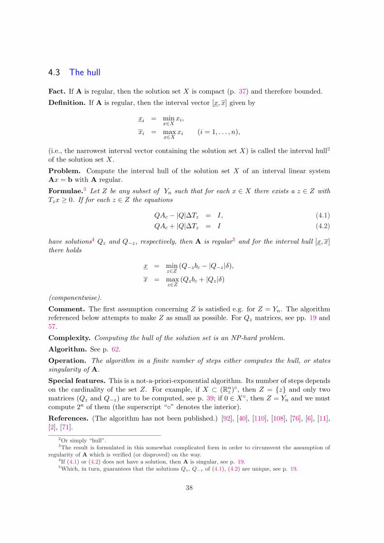
Fact. If A is regular, then the solution set X is compact (p. 37) and therefore bounded.

Definition. If A is regular, then the interval vector [x, x] given by

xi = minx∈X

xi,

xi = maxx∈X

xi (i = 1, . . . , n),

(i.e., the narrowest interval vector containing the solution set X) is called the interval hull2

of the solution set X.

Problem. Compute the interval hull of the solution set X of an interval linear systemAx = b with A regular.

Formulae.3 Let Z be any subset of Yn such that for each x ∈ X there exists a z ∈ Z withTzx ≥ 0. If for each z ∈ Z the equations

QAc − |Q|∆Tz = I, (4.1)QAc + |Q|∆Tz = I (4.2)

have solutions4 Qz and Q−z, respectively, then A is regular5 and for the interval hull [x, x]there holds

x = minz∈Z

(Q−zbc − |Q−z|δ),x = max

z∈Z(Qzbc + |Qz|δ)

(componentwise).

Comment. The first assumption concerning Z is satisfied e.g. for Z = Yn. The algorithmreferenced below attempts to make Z as small as possible. For Qz matrices, see pp. 19 and57.

Complexity. Computing the hull of the solution set is an NP-hard problem.


Operation. The algorithm in a finite number of steps either computes the hull, or statessingularity of A.

Special features. This is a not-a-priori-exponential algorithm. Its number of steps dependson the cardinality of the set Z. For example, if X ⊂ (Rn

z )◦, then Z = {z} and only twomatrices (Qz and Q−z) are to be computed, see p. 39; if 0 ∈ X◦, then Z = Yn and we mustcompute 2n of them (the superscript “◦” denotes the interior).

References. (The algorithm has not been published.) [92], [40], [110], [108], [76], [6], [11],[2], [71].

2Or simply “hull”.3The result is formulated in this somewhat complicated form in order to circumvent the assumption of

regularity of A which is verified (or disproved) on the way.4If (4.1) or (4.2) does not have a solution, then A is singular, see p. 19.5Which, in turn, guarantees that the solutions Qz, Q−z of (4.1), (4.2) are unique, see p. 19.

38

4.4 The solution set lying in a single orthant

Formulae. Let A be regular. Then X ⊂ (Rnz )◦ holds6 for some z ∈ Yn if and only if

Tz(A−1c bc) > 0, (4.3)

Tz(Q−zbc − |Q−z|δ) > 0, (4.4)Tz(Qzbc + |Qz|δ) > 0. (4.5)

In this case the hull [x, x] is given by

x = Q−zbc − |Q−z|δ, (4.6)x = Qzbc + |Qz|δ. (4.7)

Algorithm. If (4.3)- (4.5) are satisfied, then the algorithm hull (see p. 62) detects thissituation and computes the hull directly by (4.6)-(4.7).

Operation. In this case the algorithm requires computing two matrices (Qz and Q−z) only.

Special features. This is a rare case when the bounds of the hull can be given explicitlyby closed-form formulae.

References. (Unpublished.) [6], [11], [90].

6(Rnz )◦ is the interior of Rn

z .

39

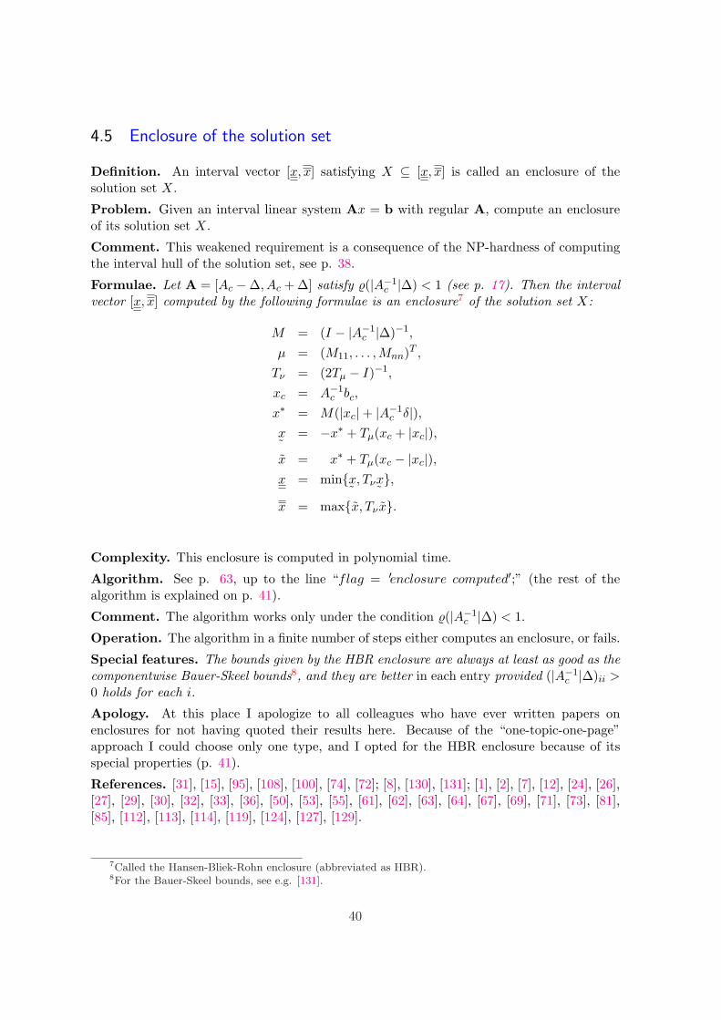
4.5 Enclosure of the solution set

Definition. An interval vector [x, x] satisfying X ⊆ [x, x] is called an enclosure of thesolution set X.

Problem. Given an interval linear system Ax = b with regular A, compute an enclosureof its solution set X.

Comment. This weakened requirement is a consequence of the NP-hardness of computingthe interval hull of the solution set, see p. 38.

Formulae. Let A = [Ac −∆, Ac + ∆] satisfy %(|A−1c |∆) < 1 (see p. 17). Then the interval

vector [x, x] computed by the following formulae is an enclosure7 of the solution set X:

M = (I − |A−1c |∆)−1,

µ = (M11, . . . ,Mnn)T ,

Tν = (2Tµ − I)−1,

xc = A−1c bc,

x∗ = M(|xc|+ |A−1c δ|),

x˜

= −x∗ + Tµ(xc + |xc|),x = x∗ + Tµ(xc − |xc|),x = min{x

˜, Tνx

˜},

x = max{x, Tν x}.

Complexity. This enclosure is computed in polynomial time.

Algorithm. See p. 63, up to the line “flag = ′enclosure computed′;” (the rest of thealgorithm is explained on p. 41).

Comment. The algorithm works only under the condition %(|A−1c |∆) < 1.

Operation. The algorithm in a finite number of steps either computes an enclosure, or fails.

Special features. The bounds given by the HBR enclosure are always at least as good as thecomponentwise Bauer-Skeel bounds8, and they are better in each entry provided (|A−1

c |∆)ii >0 holds for each i.

Apology. At this place I apologize to all colleagues who have ever written papers onenclosures for not having quoted their results here. Because of the “one-topic-one-page”approach I could choose only one type, and I opted for the HBR enclosure because of itsspecial properties (p. 41).

References. [31], [15], [95], [108], [100], [74], [72]; [8], [130], [131]; [1], [2], [7], [12], [24], [26],[27], [29], [30], [32], [33], [36], [50], [53], [55], [61], [62], [63], [64], [67], [69], [71], [73], [81],[85], [112], [113], [114], [119], [124], [127], [129].

7Called the Hansen-Bliek-Rohn enclosure (abbreviated as HBR).8For the Bauer-Skeel bounds, see e.g. [131].

40

4.6 Overestimation of the HBR enclosure

Fact. By definition (see p. 40), any enclosure [x, x] satisfies [x, x] ⊆ [x, x], where [x, x] isthe interval hull.

Problem. Determine the overestimation of the enclosure.9

Comment. Such information is usually not available. The HBR enclosure was chosen forinclusion here because of possessing this particular property.

Formulae. Under assumption and notations from p. 40, let [x, x] be the interval hull and[x, x] the HBR enclosure. Then for each i ∈ {1, . . . , n} we have

xi≤ xi ≤ x

i+ di, (4.8)

xi − di ≤ xi ≤ xi, (4.9)

where

di = eTi (I − |A−1

c Tz∆|)−1|(TzA−1c Tz − |A−1

c |)(ξi∆Mei + ∆x∗ + δ)|,

di = eTi (I − |A−1

c Tz∆|)−1|(TzA−1c Tz − |A−1

c |)(ξi∆Mei + ∆x∗ + δ)|,ξi

= (|x|+ x− xc − |xc|)i,

ξi = (|x| − x + xc − |xc|)i

and z, z are given by

zj ={

sgn (xc)j if j 6= i,−1 if j = i,

zj ={

sgn (xc)j if j 6= i,1 if j = i

(j = 1, . . . , n).

Comment. Computing d, d requires computation of up to 2n inverses (but it usually paysoff). If this number is considered too large, the matrices (I−|A−1

c Tz∆|)−1, (I−|A−1c Tz∆|)−1

in the formulae for di, di can be replaced by the matrix M , and the whole theorem will remainin force.

Complexity. Vectors d, d can be computed in polynomial time.

Algorithm. See p. 63, the lines after “flag = ′enclosure computed′;”.

Operation. The algorithm in a finite number of steps computes nonnegative vectors d, dsatisfying (4.8), (4.9).

Special features. If Ac is a diagonal matrix with positive diagonal entries, then TzA−1c Tz−

|A−1c | = TzA

−1c Tz − |A−1

c | = 0 and consequently d = d = 0, so that [x, x] = [x, x]. Hence, inthis case the HBR enclosure yields the exact interval hull.

References. (Unpublished.) [31], [15], [95], [74], [72].

9Of course, without computing the hull, which is an NP-hard problem.

41

Chapter 5

Interval linear equations and inequalities (rectangularcase)

Subject. In this chapter we consider systems of interval linear equations Ax = b (or systemsof interval linear inequalities Ax ≤ b) with a rectangular m× n interval matrix A.

42

5.1 (Z, z)-solutions

Intro. Let A = [Ac − ∆, Ac + ∆] be an m × n interval matrix and b = [bc − δ, bc + δ] aninterval m-vector. Under an interval linear system Ax = b we understand the family of allsystems Ax = b with A ∈ A, b ∈ b.

Definition. Let |Z| = E ∈ Rm×n and |z| = e ∈ Rm. A vector x ∈ Rn is said to be a(Z, z)-solution of a system Ax = b if for each Aij ∈ [Aij , Aij ] with Zij = −1 and for eachbi ∈ [bi, bi] with zi = −1 there exist Aij ∈ [Aij , Aij ] with Zij = 1 and bi ∈ [bi, bi] with zi = 1such that Ax = b holds.1

Problem. Given Z and z, describe the set of all (Z, z)-solutions of Ax = b.

Comment. Despite the complexity of the definition, it turns out that description of (Z, z)-solutions becomes wonderfully simple as soon as the Hadamard product is employed.

Formula.2 A vector x ∈ Rn is a (Z, z)-solution of Ax = b if and only if it satisfies

|Acx− bc| ≤ (Z ◦∆)|x|+ z ◦ δ. (5.1)

Complexity. Complexity of checking whether a system Ax = b has a (Z, z)-solutiondepends on the choice of Z and z; see pp. 44 and 45 for two opposite examples.

Algorithm. For verification whether a given x is a (Z, z)-solution of Ax = b, check (5.1).

Special features. This is a generalization of the Oettli-Prager theorem [77], p. 37 (whichcan be obtained from (5.1) by putting Z = E and z = e). Both its formulation and proof werenot straightforward. Shary presented his definition of (Z, z)-solutions, which he called “∀∃-solutions”, in [125]. His formulation of the result contained interval arithmetic operations.A formula not using these operations and proved from the Oettli-Prager theorem was givenin this author’s letter to Shary and Lakeyev [102]. The final step towards utmost simplicityby employing the Hadamard product was done by Lakeyev in [57].

References. [125], [57], [102], [77].

1Thus “−1” corresponds to “∀” and “1” to “∃”. It could be argued that the reverse order would be morenatural, but we would have to pay for it by introducing minus signs into the main formula (5.1).

2By Shary, Lakeyev and Rohn.

43

5.2 Tolerance solutions

Definition. A (−E, e)-solution (see p. 43) is called a tolerance solution of Ax = b. Inother words, x is a tolerance solution if it satisfies

{Ax ; A ∈ A} ⊆ b.

Problem. Describe the set of tolerance solutions of Ax = b.

Formula. For the set Xtol of tolerance solutions of Ax = b we have

Xtol = {x ; |Acx− bc| ≤ −∆|x|+ δ}= {x1 − x2 ; Ax1 −Ax2 ≤ b, Ax1 −Ax2 ≥ b, x1 ≥ 0, x2 ≥ 0}. (5.2)

Complexity. Checking whether a system Ax = b has a tolerance solution can be performedin polynomial time.

Algorithm. Use a polynomial-time linear programming algorithm to check whether thesystem of linear inequalities in (5.2) has a solution.

Operation. The algorithm in a finite number of steps checks whether Ax = b has atolerance solution (and, in the positive case, also finds such a solution).

Special features. Introduction of the notion of tolerance solutions (as early as in 1970’s)was motivated by considerations concerning crane construction [75] and input-output plan-ning with inexact data of the socialist economy of former Czechoslovakia [86].

References. [75], [86], [89], [70], [21], [47], [45], [46], [128], [118], [121], [122], [123], [58].

44

5.3 Control solutions

Definition. An (E,−e)-solution (see p. 43) is called a control solution of Ax = b. In otherwords, x is a control solution if it satisfies

b ⊆ {Ax ; A ∈ A}.

Problem. Describe the set of control solutions of Ax = b.

Formula. For the set Xcon of control solutions of Ax = b we have

Xcon = {x ; |Acx− bc| ≤ ∆|x| − δ}.

Complexity. The problem of checking whether a system Ax = b has a control solution isNP-complete.

Special features. Control solutions were introduced in [120]. The choice of the word“control” was probably motivated by the fact that each vector b ∈ b can be reached by Axwhen properly controlling the coefficients of A within A.

References. [120], [123], [126], [58], [127].

45

5.4 Strong solvability of equations

Definition. Let A = [Ac −∆, Ac + ∆] be an m× n interval matrix and b = [bc − δ, bc + δ]an interval m-vector. We say that the system Ax = b is strongly solvable if each systemAx = b with A ∈ A, b ∈ b has a solution.

Problem. Check whether a given system Ax = b is strongly solvable.

Necessary and sufficient condition. A system Ax = b is strongly solvable if and only iffor each y ∈ Ym the system3

Ayex1 −A−yex

2 = by, (5.3)

x1 ≥ 0, x2 ≥ 0 (5.4)

has a solution x1y, x2

y. Moreover, if this is the case, then for each A ∈ A, b ∈ b the systemAx = b has a solution in the set Conv{x1

y − x2y ; y ∈ Ym}.

Complexity. The problem of checking strong solvability of interval linear equations is NP-hard.


Comment. The algorithm uses a (not specified) polynomial-time linear programming sub-routine for solving the system (5.3), (5.4).

Operation. The algorithm in a finite number of steps checks strong solvability of Ax = b.

Special features. The proof of the above necessary and sufficient condition is nontrivialand uses a new existence theorem for systems of linear equations [93], [94].

References. [109], [108], [93], [94].

3Aye = Ac − Ty∆, A−ye = Ac + Ty∆ and by = bc + Tyδ, see p. 10.

46

5.5 Strong solvability of inequalities

Definition. Let A = [A,A] be an m×n interval matrix and b = [b, b] an interval m-vector.We say that the system Ax ≤ b is strongly solvable if each system Ax ≤ b with A ∈ A,b ∈ b has a solution.

Problem. Check whether a given system Ax ≤ b is strongly solvable.

Necessary and sufficient condition. A system Ax ≤ b is strongly solvable if and only ifthe system

Ax1 −Ax2 ≤ b, (5.5)

x1 ≥ 0, x2 ≥ 0 (5.6)

has a solution.

Complexity. The problem of checking strong solvability of interval linear inequalities canbe solved in polynomial time.


Comment. The algorithm uses a (not specified) polynomial-time linear programming sub-routine for solving the system (5.5), (5.6).

Operation. The algorithm in a finite number of steps checks strong solvability of Ax ≤ b.

Special features. If a system Ax ≤ b is strongly solvable, then all the systems Ax ≤ b,A ∈ A, b ∈ b, have a common solution (a nontrivial fact), which is called a strong solutionof Ax ≤ b. The algorithm on p. 65 finds a strong solution if it exists. Also, observe thedifference: checking strong solvability of interval linear equations is NP-hard, whereas thesame problem for interval linear inequalities is solvable in polynomial time.


47

Chapter 6

Interval linear programming

Subject. This last, and shortest, chapter is dedicated to a single topic, namely the rangeof the optimal value of an interval linear programming problem.

48

6.1 Reminder: optimal value of a linear program

Definition. The value1

f(A, b, c) = inf{cT x ; Ax = b, x ≥ 0}

is called the optimal value of a linear program

minimize cT x

subject toAx = b, x ≥ 0.

Comment. Hence, f(A, b, c) ∈ [−∞,∞].

Problem. Given A, b, c, compute f(A, b, c).


Algorithm. The first polynomial-time linear programming algorithm was described byKhachiyan in [48]. Many of them exist nowadays; see e.g. [78].

Special features. A polynomial-time linear programming subroutine is implicitly used inthe algorithms on pp. 64, 65 and 66.

References. [20], [48], [44], [78].

1In linear programming only finite value of f(A, b, c) is accepted as the optimal value; we use this formu-lation for the sake of utmost generality of the results.

49

6.2 Range of the optimal value

Definition. Let A = [A, A] = [Ac − ∆, Ac + ∆] be an m × n interval matrix and letb = [b, b] = [bc − δ, bc + δ] and c = [c, c] be an m-dimensional and n-dimensional intervalvector, respectively. The family of linear programming problems

min{cT x ; Ax = b, x ≥ 0} (6.1)

with data satisfyingA ∈ A, b ∈ b, c ∈ c (6.2)

is called an interval linear programming problem.

Definition. The interval [f(A,b, c), f(A,b, c)], where

f(A,b, c) = inf{f(A, b, c) ; A ∈ A, b ∈ b, c ∈ c},

f(A,b, c) = sup{f(A, b, c) ; A ∈ A, b ∈ b, c ∈ c},is called the range of the optimal value of the interval linear programming problem (6.1),(6.2).

Comment. The endpoints of [f(A,b, c), f(A,b, c)] may be ±∞.

Problem. Given A, b, c, compute [f(A,b, c), f(A,b, c)].

Formula. We have

f(A,b, c) = inf{cT x ; Ax ≤ b, Ax ≥ b, x ≥ 0},f(A,b, c) = sup

y∈Ym

f(Aye, by, c). (6.3)

Comment. Hence, solving only one linear programming problem is needed to evaluatef(A,b, c), whereas up to 2m of them are to be solved to compute f(A,b, c) according to(6.3). Although the set Ym is finite, we use “sup” here because some of the values may beinfinite. Notice the absence of any assumptions: the result is fully general.

Complexity. Computing f(A,b, c) can be performed in polynomial time, whereas compu-tation of f(A,b, c) is NP-hard.


Operation. The algorithm computes the range of the optimal value in a finite number ofsteps.

Special features. If f(A,b, c) is finite, then

f(A,b, c) = sup{bTc p + δT |p| ; AT

c p−∆T |p| ≤ c},

so that in this case the upper bound can be computed by solving one nonlinear programmingproblem.

References. [87], [88], [108], [59], [52], [13], [65], [66], [37], [38], [39], [42], [98], [88], [49],[51], [67], [82], [132].

50

Chapter 7

Algorithms

Subject. Here we give MATLAB-like descriptions of fifteen basic algorithms that have beenreferred to in the previous chapters.

Scheme. The following scheme demonstrates the interdependence of the algorithms (a → bmeans that the algorithm a is used as a subroutine in the algorithm b). It explains thecentral role played by the algorithms ynset, signaccord and hull.

norminfone↑

ynset −→ strosolveq↓ ↑

range ←− linear programming −→ strosolvin

signaccord −→ qzmatrix −→ hull −→ inverse↓

regularity −→ posdefness −→ hurwitzstab↓

schurstab

The algorithms singular and hbr do not use subroutines.

Algorithm description. For algorithm form, see p. 6. In particular, [ ] denotes the emptymatrix or vector (which is not used in linear algebra, but is a useful programming tool); itis assigned to matrices or vectors that have not been computed.

51

7.1 An algorithm for generating the set Yn

function Y = ynset(n)z = 0 ∈ Rn; y = e ∈ Rn; Y = {y};while z 6= e

k = min{i ; zi = 0};for i = 1 : k − 1, zi = 0; endzk = 1;yk = −yk;Y = Y ∪ {y};

end

Figure 7.1: An algorithm for generating the set Yn (p. 12).

52

7.2 An algorithm for computing the norm ‖A‖∞,1

function ν = norminfone (A)y = e ∈ Rn; z = 0 ∈ Rn−1;x = Ay;ν = ‖x‖1;while z 6= e

k = min{i ; zi = 0};x = x− 2ykA•k;ν = max{ν, ‖x‖1};for i = 1 : k − 1, zi = 0; endzk = 1;yk = −yk;

end

Figure 7.2: An algorithm for computing the norm ‖A‖∞,1 (p. 13).

53

7.3 The sign accord algorithm

function [x, flag, As] = signaccord (A,B, b)% Finds a solution to Ax + B|x| = b or states% singularity of [A− |B|, A + |B|].x = [ ]; flag = ′singular′; As = [ ];if A is singular, As = A; return, endp = 0 ∈ Rn;x = A−1b;z = sgnx;if A + BTz is singular, As = A + BTz; x = [ ]; return, endx = (A + BTz)−1b;C = −(A + BTz)−1B;while zjxj < 0 for some j

k = min{j ; zjxj < 0};if 1 + 2zkCkk ≤ 0

τ = (−1)/(2zkCkk);As = A + B(Tz − 2τzkeke

Tk );

x = [ ];return

endpk = pk + 1;zk = −zk;if log2 pk > n− k, x = [ ]; return, endα = 2zk/(1− 2zkCkk);x = x + αxkC•k;C = C + αC•kCk•;

endflag = ′solution found′;

Figure 7.3: The sign accord algorithm (p. 14).

Comment. After each updating of x and C there holds x = (A + BTz)−1b and C =−(A + BTz)−1B for the current z. The variable pk registers the number of occurrences of k;if pk > 2n−k for some k, then [A− |B|, A + |B| ] is singular (see [92]).

54

7.4 An algorithm for checking regularity

function flag = regularity (A)if Ac is singular, flag = ′singular′; return, endR = A−1

c ;if %(|R|∆) < 1, flag = ′regular′; return, endif maxj(|R|∆)jj ≥ 1, flag = ′singular′; return, endb = e; γ = mink |Rb|k;for i = 1 : n

for j = 1 : nb′ = b; b′j = −b′j ;if mink |Rb′|k > γ, γ = mink |Rb′|k; b = b′; end

endend[x, x, flag] = hull (A, [b, b]);if flag = ′hull computed′, flag = ′regular′; returnend

Figure 7.4: An algorithm for checking regularity (p. 17).

Comment. Both the for loops may be omitted without affecting functioning of the algo-rithm. They form only an empirical tool [41] aimed at diminishing the number of orthantsto be visited by the subroutine hull.

55

7.5 An algorithm for finding a singular matrix

function [flag,As] = singular (A)flag = ′singular′; As = [ ];if Ac is singular, As = Ac; return, endy = e ∈ Rn; z = e ∈ Rn; t = 0 ∈ R2n−1;if A is singular, As = A; return, endD = A−1;while t 6= e

k = min{i ; ti = 0};for i = 1 : k − 1, ti = 0; endtk = 1;if k ≤ n

i = k; p = eTi AcD − eT

i ;if 2pi + 1 ≤ 0

τ = −yi/(2pi);As = Ac − (Ty − 2τeie

Ti )∆Tz; return

endα = 2/(2pi + 1);D = D − αDeip;yi = −yi;

elsej = k − n; p = DAcej − ej ;if 2pj + 1 ≤ 0

τ = −zj/(2pj);As = Ac − Ty∆(Tz − 2τeje

Tj ); return

endα = 2/(2pj + 1);D = D − αpeT

j D;zj = −zj ;

endendflag = ′regular′;

Figure 7.5: An algorithm for finding a singular matrix (p. 18).

Comment. After each updating of y or z there holds D = A−1yz .

56

7.6 An algorithm for computing Qz

function [Qz, f lag] = qzmatrix (A, z)for i = 1 : n

[x, flag] = signaccord (ATc ,−Tz∆T , ei);

if flag = ′singular′, Qz = [ ]; returnend(Qz)i• = xT ;

endflag = ′solution computed′;

Figure 7.6: An algorithm for computing Qz (p. 19).

57

7.7 An algorithm for computing the inverse

function [B, B, flag] = inverse (A)for j = 1 : n

[x, x, flag] = hull (A, [ej , ej ]);if flag = ′singular′, B = [ ]; B = [ ]; returnendB•j = x; B•j = x;

endflag = ′inverse computed′;

Figure 7.7: An algorithm for computing the inverse (p. 20).

58

7.8 An algorithm for checking positive definiteness

function flag = posdefness (A)if Ac is not positive definite

flag = ′not positive definite′; returnendif λmin(Ac) > %(∆)

flag = ′positive definite′; returnendflag = regularity (A);if flag = ′regular′, flag = ′positive definite′; returnelse flag = ′not positive definite′; returnend

Figure 7.8: An algorithm for checking positive definiteness (p. 31).

59

7.9 An algorithm for checking Hurwitz stability

function flag = hurwitzstab (A)A′c = (Ac + AT

c )/2; ∆′ = (∆ + ∆T )/2;flag = posdefness ([−A′c −∆′,−A′c + ∆′]);if flag = ′positive definite′

flag = ′Hurwitz stable′; returnelse

if (A′c = Ac and ∆′ = ∆)flag = ′not Hurwitz stable′; return

elseflag = ′Hurwitz stability not verified′; return

endend

Figure 7.9: An algorithm for checking Hurwitz stability (p. 32).

60

7.10 An algorithm for checking Schur stability

function flag = schurstab (A)if (AT

c 6= Ac or ∆T 6= ∆)flag = ′Schur stability not verified′; return

endflag = hurwitzstab ([Ac − I −∆, Ac − I + ∆]);if flag = ′not Hurwitz stable′

flag = ′not Schur stable′; returnendflag = hurwitzstab ([−Ac − I −∆,−Ac − I + ∆]);if flag = ′not Hurwitz stable′

flag = ′not Schur stable′; returnendflag = ′Schur stable′;

Figure 7.10: An algorithm for checking Schur stability (p. 33).

61

7.11 An algorithm for computing the hull

function [x, x, flag] = hull (A,b)if Ac is singular

x = [ ]; x = [ ]; flag = ′singular′; returnendx = A−1

c bc; x = x;z = sgnx; Z = {z}; D = ∅;while Z 6= ∅

select z ∈ Z; Z = Z − {z}; D = D ∪ {z};[Q−z, f lag] = qzmatrix(A,−z);if flag = ′singular′, x = [ ]; x = [ ]; return, endx˜

= Q−zbc − |Q−z|δ;[Qz, f lag] = qzmatrix(A, z);if flag = ′singular′, x = [ ]; x = [ ]; return, endx = Qzbc + |Qz|δ;if x

˜≤ x

x = min{x, x˜};

x = max{x, x};for j = 1 : n

z′ = z; z′j = −z′j ;if (x

˜j xj ≤ 0 and z′ /∈ Z ∪D), Z = Z ∪ {z′}; end

endend

endflag = ′hull computed′;

Figure 7.11: An algorithm for computing the hull (p. 38).

Comment. Z is the set of sign vectors of orthants to be visited; D is the set of those thatalready have been visited.

62

7.12 The Hansen-Bliek-Rohn enclosure algorithm

function [x, x, d, d, flag] = hbr (A,b)if (Ac is singular or I − |A−1

c |∆ is singular or (I − |A−1c |∆)−1 6≥ I)

x = [ ]; x = [ ]; d = [ ]; d = [ ]; flag = ′enclosure not computed′;return

endM = (I − |A−1

c |∆)−1;µ = (M11, . . . , Mnn)T ;Tν = (2Tµ − I)−1;xc = A−1

c bc;x∗ = M(|xc|+ |A−1

c δ|);x˜

= −x∗ + Tµ(xc + |xc|);x = x∗ + Tµ(xc − |xc|);x = max{x, Tν x};x = min{x

˜, Tνx

˜};

flag = ′enclosure computed′;z = sgnxc;ξ = |x| − x + xc − |xc|;ξ = |x|+ x− xc − |xc|;for i = 1 : n

z′ = z; z′i = −1; N = (I − |A−1c Tz′∆|)−1;

di = (N |(Tz′A−1c Tz′ − |A−1

c |)(ξi∆Mei + ∆x∗ + δ)|)i;

z′i = 1; N = (I − |A−1c Tz′∆|)−1;

di = (N |(Tz′A−1c Tz′ − |A−1

c |)(ξi∆Mei + ∆x∗ + δ)|)i;end

Figure 7.12: The Hansen-Bliek-Rohn enclosure algorithm (pp. 40, 41).

63

7.13 An algorithm for checking strong solvability of equations

At the start of the algorithm the equations of the system Ax = b should be reordered insuch a way that the matrix (∆ δ) has first q rows nonzero (0 ≤ q ≤ m) and the remainingm− q rows zero.

function flag = strosolveq(A,b)reorder the equations;z = 0 ∈ Rq; y = e ∈ Rq; flag = ′strongly solvable′;A = A; B = A; b = b;if Ax1 −Bx2 = b, x1 ≥ 0, x2 ≥ 0 is not solvable

flag = ′not strongly solvable′; returnendwhile z 6= e

k = min{i ; zi = 0};for i = 1 : k − 1, zi = 0; endzk = 1;yk = −yk;if yk = 1

Ak• = Ak•; Bk• = Ak•; bk = bk;else

Ak• = Ak•; Bk• = Ak•; bk = bk;endif Ax1 −Bx2 = b, x1 ≥ 0, x2 ≥ 0 is not solvable

flag = ′not strongly solvable′; returnend

end

Figure 7.13: An algorithm for checking strong solvability of equations (p. 46).

Comment. After each updating of A, B and b there holds A = Aye, B = A−ye, b = by forthe current y.

64

7.14 An algorithm for checking strong solvability of inequalities

function [x, flag] = strosolvin(A,b)solve the system Ax1 −Ax2 ≤ b, x1 ≥ 0, x2 ≥ 0;if it has a solution x1, x2

x = x1 − x2; flag = ′strong solution found′;else

x = [ ]; flag = ′not strongly solvable′;end

Figure 7.14: An algorithm for checking strong solvability of inequalities (p. 47).

65

7.15 An algorithm for computing the range of the optimal value

At the start of the algorithm the equations of the system Ax = b should be reordered insuch a way that the matrix (∆ δ) has first q rows nonzero (0 ≤ q ≤ m) and the remainingm− q rows zero.

function [f, f, flag] = range(A,b, c)reorder the equations;compute f = inf{cT x ; Ax ≤ b, Ax ≥ b, x ≥ 0};z = 0 ∈ Rq; y = e ∈ Rq;A = A; b = b; f = f(A, b, c);while (z 6= e and f < ∞)

k = min{i ; zi = 0};for i = 1 to k − 1, zi = 0; endzk = 1;yk = −yk;if yk = 1

Ak• = Ak•; bk = bk;else

Ak• = Ak•; bk = bk;endf = max{f, f(A, b, c)};

endflag = ′range computed′;

Figure 7.15: An algorithm for computing the range of the optimal value (p. 50).

Comment. After each updating of A and b there holds A = Aye, b = by for the current y.

66

Bibliography

[1] J. Albrecht, Monotone Iterationsfolgen und ihre Verwendung zur Losung linearer Gle-ichungssysteme, Numerische Mathematik, 3 (1961), pp. 345–358. 40

[2] G. Alefeld and J. Herzberger, Introduction to Interval Computations, Academic Press,New York, 1983. 38, 40

[3] B. R. Barmish, New Tools for Robustness of Linear Systems, MacMillan, New York,1994. 25

[4] B. R. Barmish and C. V. Hollot, Counter-example to a recent result on the stability ofinterval matrices by S. BiaÃlas, International Journal of Control, 39 (1984), pp. 1103–1104. 32

[5] I. Bar-On, B. Codenotti and M. Leoncini, Checking robust nonsingularity of tridiagonalmatrices in linear time, BIT, 36 (1996), pp. 206–220. 25

[6] W. Barth and E. Nuding, Optimale Losung von Intervallgleichungssystemen, Comput-ing, 12 (1974), pp. 117–125. 1, 38, 39

[7] H. Bauch, K.-U. Jahn, D. Oelschlagel, H. Susse, and V. Wiebigke, Intervallmathematik,Teubner, Leipzig, 1987. 40

[8] F. L. Bauer, Genauigkeitsfragen bei der Losung linearer Gleichungssysteme, Zeitschriftfur Angewandte Mathematik und Mechanik, 46 (1966), pp. 409–421. 40

[9] M. Baumann, A regularity criterion for interval matrices, in Collection of Scientific Pa-pers Honouring Prof. Dr. K. Nickel on Occasion of his 60th Birthday, Part I, J. Garloffet al., eds., Freiburg, 1984, Albert-Ludwigs-Universitat, pp. 45–50. 17

[10] H. Beeck, Charakterisierung der Losungsmenge von Intervallgleichungssystemen,Zeitschrift fur Angewandte Mathematik und Mechanik, 53 (1973), pp. T181–T182.37

[11] H. Beeck, Zur scharfen Aussenabschatzung der Losungsmenge bei linearen Intervall-gleichungssystemen, Zeitschrift fur Angewandte Mathematik und Mechanik, 54 (1974),pp. T208–T209. 38, 39

[12] H. Beeck, Zur Problematik der Hullenbestimmung von Intervallgleichungssystemen, inInterval Mathematics, K. Nickel, ed., Lecture Notes in Computer Science 29, Berlin,1975, Springer-Verlag, pp. 150–159. 17, 40

67

[13] H. Beeck, Linear programming with inexact data, Technical Report TUM–ISU–7830,Technical University of Munich, Munich, 1978. 50

[14] S. BiaÃlas, A necessary and sufficient condition for the stability of interval matrices,International Journal of Control, 37 (1983), pp. 717–722. 32

[15] C. Bliek, Computer Methods for Design Automation, PhD thesis, Massachusetts Insti-tute of Technology, Cambridge, MA, July 1992. 40, 41

[16] R. D. Braatz, P. M. Young, J. C. Doyle and M. Morari, Computational complexity ofmu calculation, IEEE Transactions on Automatic Control, 39 (1994), pp. 1000–1002.25

[17] G. F. Corliss, Industrial applications of interval techniques, in Computer Arithmeticand Self-Validating Numerical Methods, C. Ullrich, ed., no. 7 in Notes and Reports inMathematics in Science and Engineering, San Diego, 1990, Academic Press, pp. 91–113. 21

[18] G. E. Coxson, Computing exact bounds on elements of an inverse interval matrix isNP-hard, Reliable Computing, 5 (1999), pp. 137–142. 20

[19] G. E. Coxson and C. L. DeMarco, Computing the real structured singular value is NP-hard, Report ECE-92-4, Department of Electrical and Computer Engineering, Univer-sity of Wisconsin, Madison, 1992. 25

[20] G. Dantzig, Linear Programming and Extensions, Princeton University Press, Prince-ton, 1963. 49

[21] A. Deif, Sensitivity Analysis in Linear Systems, Springer-Verlag, Berlin, 1986. 44

[22] J. W. Demmel, The componentwise distance to the nearest singular matrix, SIAMJournal on Matrix Analysis and Applications, 13 (1992), pp. 10–19. 25

[23] J. C. Doyle, Analysis of feedback systems with structured uncertainties, IEE Proceed-ings, Part D, 129 (1982), pp. 242–250. 25

[24] A. Frommer and G. Mayer, A new criterion to guarantee the feasibility of the intervalGaussian algorithm, SIAM Journal on Matrix Analysis and Applications, 14 (1993),pp. 408–419. 40

[25] M. R. Garey and D. S. Johnson, Computers and Intractability: A Guide to the Theoryof NP-Completeness, Freeman, San Francisco, 1979. 13

[26] J. Garloff, Totally nonnegative interval matrices, in Interval Mathematics 1980,K. Nickel, ed., New York, 1980, Academic Press, pp. 317–327. 23, 40

[27] D. Gay, Solving interval linear equations, SIAM Journal on Numerical Analysis, 19(1982), pp. 858–870. 40

[28] G. H. Golub and C. F. van Loan, Matrix Computations, The Johns Hopkins UniversityPress, Baltimore, 1996. 29

68

[29] E. Hansen, On linear algebraic equations with interval coefficients, in Topics in IntervalAnalysis, E. Hansen, ed., Oxford, 1969, Oxford University Press, pp. 33–46. 40

[30] E. Hansen, On the solution of linear algebraic equations with interval coefficients, Lin-ear Algebra and Its Applications, 2 (1969), pp. 153–165. 40

[31] E. R. Hansen, Bounding the solution of interval linear equations, SIAM Journal onNumerical Analysis, 29 (1992), pp. 1493–1503. 40, 41

[32] G. Heindl, Some inclusion results based on a generalized version of the Oettli-Pragertheorem, Zeitschrift fur Angewandte Mathematik und Mechanik, Supplement 3, 76(1996), pp. 263–266. 40

[33] G. Heindl, An improvement of the componentwise error estimate corresponding to awell-known inclusion result for solutions of systems of linear equations, in Recent Ad-vances in Numerical Methods and Applications, O. P. Iliev, ed., Singapore, 1999, WorldScientific, pp. 355–361. 40

[34] J. Herzberger and D. Bethke, On two algorithms for bounding the inverse of an intervalmatrix, Interval Computations, 1 (1991), pp. 44–53. 21

[35] N. J. Higham, Accuracy and Stability of Numerical Algorithms, SIAM, Philadelphia,1996. 13

[36] K.-U. Jahn, Eine Theorie der Gleichungssysteme mit Intervallkoeffizienten, Zeitschriftfur Angewandte Mathematik und Mechanik, 54 (1974), pp. 405–412. 40

[37] C. Jansson, Zur linearen Optimierung mit unscharfen Daten, PhD thesis, Universityof Kaiserslautern, 1985. 50

[38] C. Jansson, A self-validating method for solving linear programming problems withinterval input data, Computing Supplementum, 6 (1988), pp. 33–46. 50

[39] C. Jansson, On self-validating methods for optimization problems, in Topics in Vali-dated Computations, J. Herzberger, ed., Amsterdam, 1994, North-Holland, pp. 381–438. 50

[40] C. Jansson, Calculation of exact bounds for the solution set of linear interval systems,Linear Algebra and Its Applications, 251 (1997), pp. 321–340. 37, 38

[41] C. Jansson and J. Rohn, An algorithm for checking regularity of interval matri-ces, SIAM Journal on Matrix Analysis and Applications, 20 (1999), pp. 756–776.http://www.cs.cas.cz/˜rohn/publist/95.ps 17, 55

[42] C. Jansson and S. M. Rump, Rigorous solution of linear programming problems withuncertain data, ZOR-Methods and Models of Operations Research, 35 (1991), pp. 87–111. 50

[43] W. C. Karl, J. P. Greschak, and G. C. Verghese, Comments on “A necessary and suffi-cient condition for the stability of interval matrices”, International Journal of Control,39 (1984), pp. 849–851. 32

69

http://www.cs.cas.cz/~rohn/publist/95.ps�

[44] N. Karmarkar, A new polynomial-time algorithm for linear programming, Combinator-ica, 4 (1984), pp. 373–395. 49

[45] B. Kelling, Methods of solution of linear tolerance problems with interval arithmetic, inComputer Arithmetic and Enclosure Methods, L. Atanassova and J. Herzberger, eds.,Amsterdam, 1992, North-Holland, pp. 269–277. 44

[46] B. Kelling, Geometrische Untersuchungen zur eingeschrankten Losungsmenge linearerIntervallgleichungssysteme, Zeitschrift fur Angewandte Mathematik und Mechanik, 74(1994), pp. 625–628. 44

[47] B. Kelling and D. Oelschlagel, Zur Losung von linearen Toleranzproblemen, Wis-senschaftliche Zeitschrift TH Leuna-Merseburg, 33 (1991), pp. 121–131. 44

[48] L. G. Khachiyan, A polynomial algorithm in linear programming, Doklady AkademiiNauk SSSR, 244 (1979), pp. 1093–1096. 49

[49] J. Konıckova, Optimalizacnı ulohy s nepresnymi daty, PhD thesis, Charles University,Prague, 1996. 50

[50] J. Konıckova, Solution of systems of interval linear equations, Zeitschrift fur Ange-wandte Mathematik und Mechanik, Supplement 3, 80 (2000), pp. S807–S808. 40

[51] J. Konıckova, Sufficient condition of basis stability of an interval linear programmingproblem, Zeitschrift fur Angewandte Mathematik und Mechanik, Supplement 3, 81(2001), pp. S677–S678. 50

[52] R. Krawczyk, Fehlerabschatzung bei linearer Optimierung, in Interval Mathematics,K. Nickel, ed., Lecture Notes in Computer Science 29, Berlin, 1975, Springer-Verlag,pp. 215–222. 50

[53] R. Krawczyk, Intervalliterationsverfahren, Bericht 186, Mathematisch-Statistische Sek-tion im Forschungszentrum Graz, Graz, 1982. 40

[54] V. Kreinovich, A. Lakeyev, J. Rohn, and P. Kahl, Computational Complexity and Fea-sibility of Data Processing and Interval Computations, Kluwer Academic Publishers,Dordrecht, 1998. 30

[55] I. Kuperman, Approximate Linear Algebraic Equations and Roundoff Error Estimation,PhD thesis, University of Witwatersrand, Johannesburg, 1967. 40

[56] J. Kuttler, A fourth-order finite-difference approximation for the fixed membrane eigen-problem, Mathematics of Computation, 25 (1971), pp. 237–256. 24

[57] A. V. Lakeyev, Vychislitel’naya slozhnost’ ocenivaniya obobshchennykh mnozhestv resh-eniy interval’nych lineynykh sistem, in Trudy XI mezhdunarodnoi Baikalskoi shkoly-seminara “Metody optimizacii i ich prilozheniya”, Irkutsk, 1998, pp. 115–118. 43

[58] A. V. Lakeyev and S. I. Noskov, On the set of solutions of a linear equation withintervally defined operator and right-hand side (in Russian), Siberian MathematicalJournal, 35 (1994), pp. 1074–1084. 44, 45

70

[59] B. Machost, Numerische Behandlung des Simplexverfahrens mit intervallanalytischenMethoden, Berichte der GMD, GMD, Bonn, 1970. 50

[60] M. Mansour, Robust stability of interval matrices, Proceedings of the 28th Conferenceon Decision and Control, Tampa, FL, (1989), pp. 46–51. 32

[61] G. Mayer, Epsilon-inflation in verification algorithms, Journal of Computational andApplied Mathematics, 60 (1995), pp. 147–169. 40

[62] G. Mayer and J. Rohn, On the applicability of the interval Gaussian algorithm, ReliableComputing, 4 (1998), pp. 205–222. http://www.cs.cas.cz/˜rohn/publist/mayer.ps 40

[63] R. E. Moore, Interval Analysis, Prentice-Hall, Englewood Cliffs, 1966. 40

[64] R. E. Moore, Methods and Applications of Interval Analysis, SIAM Studies in AppliedMathematics, SIAM, Philadelphia, 1979. 40

[65] F. Mraz, Uloha linearnıho programovanı s intervalovymi koeficienty. West BohemianUniversity, 1993. Habilitationsschrift. 50

[66] F. Mraz, Calculating the exact bounds of optimal values in LP with interval coefficients,Annals of Operations Research, 81 (1998), pp. 51–62. 50

[67] J. Nedoma, Vague matrices in linear programming, Annals of Operations Research, 47(1993), pp. 483–496. 40, 50

[68] A. Nemirovskii, Several NP-hard problems arising in robust stability analysis, Mathe-matics of Control, Signals, and Systems, 6 (1993), pp. 99–105. 32

[69] A. Neumaier, Linear interval equations, in Interval Mathematics 1985, K. Nickel, ed.,Lecture Notes in Computer Science 212, Berlin, 1985, Springer-Verlag, pp. 109–120.40

[70] A. Neumaier, Tolerance analysis with interval arithmetic, Freiburger Intervall-Berichte86/9, Albert-Ludwigs-Universitat, Freiburg, 1986. 44

[71] A. Neumaier, Interval Methods for Systems of Equations, Cambridge University Press,Cambridge, 1990. 37, 38, 40

[72] A. Neumaier, A simple derivation of the Hansen-Bliek-Rohn-Ning-Kearfott enclosurefor linear interval equations, Reliable Computing, 5 (1999), pp. 131–136. 40, 41

[73] K. Nickel, Die Uberschatzung des Wertebereichs einer Funktion in der Intervallrech-nung mit Anwendungen auf lineare Gleichungssysteme, Computing, 18 (1977), pp. 15–36. 40

[74] S. Ning and R. B. Kearfott, A comparison of some methods for solving linear intervalequations, SIAM Journal on Numerical Analysis, 34 (1997), pp. 1289–1305. 40, 41

[75] E. Nuding and J. Wilhelm, Uber Gleichungen und uber Losungen, Zeitschrift fur Ange-wandte Mathematik und Mechanik, 52 (1972), pp. T188–T190. 44

71

http://www.cs.cas.cz/~rohn/publist/mayer.ps�

[76] W. Oettli, On the solution set of a linear system with inaccurate coefficients, SIAMJournal on Numerical Analysis, 2 (1965), pp. 115–118. 38

[77] W. Oettli and W. Prager, Compatibility of approximate solution of linear equationswith given error bounds for coefficients and right-hand sides, Numerische Mathematik,6 (1964), pp. 405–409. 37, 43

[78] M. Padberg, Linear Optimization and Extensions, Springer-Verlag, Berlin, 1999. 49

[79] S. Poljak and J. Rohn, Radius of nonsingularity, Research Report, KAM Series 88–117, Faculty of Mathematics and Physics, Charles University, Prague, December 1988.http://www.cs.cas.cz/˜rohn/publist/38.doc 25

[80] S. Poljak and J. Rohn, Checking robust nonsingularity is NP-hard, Mathematics of Con-trol, Signals, and Systems, 6 (1993), pp. 1–9. http://www.cs.cas.cz/˜rohn/publist/63.doc25

[81] K. Reichmann, Abbruch beim Intervall-Gauss-Algorithmus, Computing, 22 (1979),pp. 355–361. 40

[82] J. Renegar, Some perturbation theory for linear programming, Mathematical Program-ming, 65 (1994), pp. 73–91. 50

[83] G. Rex and J. Kupferschmidt, What is the radius of singularity of a real matrix?,Zeitschrift fur Angewandte Mathematik und Mechanik, 81 (2001), pp. 985–986. 25

[84] G. Rex and J. Rohn, Sufficient conditions for regularity and singularity of intervalmatrices, SIAM Journal on Matrix Analysis and Applications, 20 (1999), pp. 437–445.http://www.cs.cas.cz/˜rohn/publist/94.ps 26

[85] H.-G. Rex, Zur Losungseinschließung linearer Gleichungssysteme, WissenschaftlicheZeitschrift, Technische Hochschule Leipzig, 15 (1991), pp. 441–447. 40

[86] J. Rohn, Input-output planning with inexact data, Freiburger Intervall-Berichte 78/9,Albert-Ludwigs-Universitat, Freiburg, 1978. http://www.cs.cas.cz/˜rohn/publist/11.doc44

[87] J. Rohn, Duality in interval linear programming, in Interval Mathemat-ics 1980, K. Nickel, ed., New York, 1980, Academic Press, pp. 521–529.http://www.cs.cas.cz/˜rohn/publist/12.doc 50

[88] J. Rohn, Interval linear systems, Freiburger Intervall-Berichte 84/7, Albert-Ludwigs-Universitat, Freiburg, 1984. http://www.cs.cas.cz/˜rohn/publist/25.doc 50

[89] J. Rohn, Inner solutions of linear interval systems, in Interval Mathematics 1985,K. Nickel, ed., Lecture Notes in Computer Science 212, Berlin, 1986, Springer-Verlag,pp. 157–158. http://www.cs.cas.cz/˜rohn/publist/31.doc 44

[90] J. Rohn, Inverse-positive interval matrices, Zeitschrift fur Angewandte Mathematikund Mechanik, 67 (1987), pp. T492–T493. http://www.cs.cas.cz/˜rohn/publist/32.doc 24,39

72

http://www.cs.cas.cz/~rohn/publist/38.doc�








[91] J. Rohn, Nearness of matrices to singularity, Research Report, KAM Series88–79, Faculty of Mathematics and Physics, Charles University, Prague, 1988.http://www.cs.cas.cz/˜rohn/publist/37.doc 25

[92] J. Rohn, Systems of linear interval equations, Linear Algebra and Its Applications, 126(1989), pp. 39–78. http://www.cs.cas.cz/˜rohn/publist/47.doc 14, 17, 18, 19, 20, 22, 23,26, 38, 54

[93] J. Rohn, Characterization of a linear program in standard form by a family of lin-ear programs with inequality constraints, Ekonomicko-matematicky obzor, 26 (1990),pp. 71–73. http://www.cs.cas.cz/˜rohn/publist/49.doc 46

[94] J. Rohn, An existence theorem for systems of linear equations, Linear and MultilinearAlgebra, 29 (1991), pp. 141–144. http://www.cs.cas.cz/˜rohn/publist/54.doc 46

[95] J. Rohn, Cheap and tight bounds: The recent result by E. Hansen canbe made more efficient, Interval Computations, 4 (1993), pp. 13–21.http://www.cs.cas.cz/˜rohn/publist/69.ps 21, 40, 41

[96] J. Rohn, Interval matrices: Singularity and real eigenvalues, SIAMJournal on Matrix Analysis and Applications, 14 (1993), pp. 82–91.http://www.cs.cas.cz/˜rohn/publist/61.doc 18, 26, 27, 28

[97] J. Rohn, Inverse interval matrix, SIAM Journal on Numerical Analysis, 30 (1993),pp. 864–870. http://www.cs.cas.cz/˜rohn/publist/65.doc 20, 22

[98] J. Rohn, Stability of the optimal basis of a linear program under uncertainty, OperationsResearch Letters, 13 (1993), pp. 9–12. http://www.cs.cas.cz/˜rohn/publist/64.doc 50

[99] J. Rohn, Checking positive definiteness or stability of symmetric interval matrices isNP-hard, Commentationes Mathematicae Universitatis Carolinae, 35 (1994), pp. 795–797. http://www.cs.cas.cz/˜rohn/publist/74.ps 29, 31, 32, 33

[100] J. Rohn, A perturbation theorem for linear equations, Commentationes MathematicaeUniversitatis Carolinae, 35 (1994), pp. 213–214. http://www.cs.cas.cz/˜rohn/publist/77.ps40

[101] J. Rohn, Positive definiteness and stability of interval matrices, SIAMJournal on Matrix Analysis and Applications, 15 (1994), pp. 175–184.http://www.cs.cas.cz/˜rohn/publist/68.doc 30, 31, 32, 33

[102] J. Rohn. E-mail letter to S. P. Shary and A. V. Lakeyev of November 18, 1995.http://www.cs.cas.cz/˜rohn/publist/LettShaLak.ps 43

[103] J. Rohn, Checking properties of interval matrices, Technical Report 686, Institute ofComputer Science, Academy of Sciences of the Czech Republic, Prague, September1996. http://www.cs.cas.cz/˜rohn/publist/92.ps 29

[104] J. Rohn, Enclosing solutions of overdetermined systems of linear interval equations,Reliable Computing, 2 (1996), pp. 167–171. http://www.cs.cas.cz/˜rohn/publist/88.ps 34

73












http://www.cs.cas.cz/~rohn/publist/LettShaLak.ps�



[105] J. Rohn, Complexity of some linear problems with interval data, Reliable Computing,3 (1997), pp. 315–323. http://www.cs.cas.cz/˜rohn/publist/96.ps 13

[106] J. Rohn, Bounds on eigenvalues of interval matrices, Zeitschrift fur Ange-wandte Mathematik und Mechanik, Supplement 3, 78 (1998), pp. S1049–S1050.http://www.cs.cas.cz/˜rohn/publist/97.ps 29

[107] J. Rohn, Computing the norm ‖A‖∞,1 is NP-hard, Linear and Multilinear Algebra, 47(2000), pp. 195–204. http://www.cs.cas.cz/˜rohn/publist/norm.ps 13

[108] J. Rohn, Systems of interval linear equations and inequalities (rectangular case), Tech-nical Report 875, Institute of Computer Science, Academy of Sciences of the CzechRepublic, Prague, September 2002. http://www.cs.cas.cz/˜rohn/publist/chapters.ps 12,13, 21, 37, 38, 40, 46, 47, 50

[109] J. Rohn, Solvability of systems of linear interval equations, SIAM Jour-nal on Matrix Analysis and Applications, 25 (2003), pp. 237–245.http://www.cs.cas.cz/˜rohn/publist/solvability.pdf 46

[110] J. Rohn and V. Kreinovich, Computing exact componentwise bounds on solutions oflinear systems with interval data is NP-hard, SIAM Journal on Matrix Analysis andApplications, 16 (1995), pp. 415–420. http://www.cs.cas.cz/˜rohn/publist/72.ps 17, 38

[111] J. Rohn and J. Kreslova, Linear interval inequalities, Linear and Multilinear Algebra,38 (1994), pp. 79–82. http://www.cs.cas.cz/˜rohn/publist/71.ps 47

[112] S. M. Rump, Solving algebraic problems with high accuracy, in A New Approach toScientific Computation, U. Kulisch and W. Miranker, eds., New York, 1983, AcademicPress, pp. 51–120. 40

[113] S. M. Rump, On the solution of interval linear systems, Computing, 47 (1992), pp. 337–353. 40

[114] S. M. Rump, Verification methods for dense and sparse systems of equations, in Top-ics in Validated Computations, J. Herzberger, ed., Amsterdam, 1994, North-Holland,pp. 63–135. 40

[115] S. M. Rump, The distance between regularity and strong regularity, in Scientific Com-puting and Validated Numerics, G. Alefeld, A. Frommer and B. Lang, eds., Mathe-matical Research, Vol. 90, Berlin, 1996, Akademie Verlag, pp. 105–117. 25

[116] S. M. Rump, Bounds for the componentwise distance to the nearest singular matrix,SIAM Journal on Matrix Analysis and Applications, 18 (1997), pp. 83–103. 25

[117] S. M. Rump, Almost sharp bounds for the componentwise distance to the nearest sin-gular matrix, Linear and Multilinear Algebra, 42 (1998), pp. 93–108. 25

[118] S. P. Shary, O nekotorykh metodakh resheniya lineinoi zadachi o dopuskakh, Preprint 6,Siberian Branch of the Soviet Academy of Sciences, Krasnoyarsk, 1989. 44

74



http://www.cs.cas.cz/~rohn/publist/norm.ps�

http://www.cs.cas.cz/~rohn/publist/chapters.ps�

http://www.cs.cas.cz/~rohn/publist/solvability.pdf�



[119] S. P. Shary, A new class of algorithms for optimal solution of interval linear systems,Interval Computations, 2 (1992), pp. 18–29. 40

[120] S. P. Shary, On controlled solution set of interval algebraic systems, Interval Compu-tations, 6 (1992), pp. 66–75. 45

[121] S. P. Shary, Solving the tolerance problem for interval linear systems, Interval Compu-tations, 2 (1994), pp. 6–26. 44

[122] S. P. Shary, Solving the linear interval tolerance problem, Mathematics and Computersin Simulation, 39 (1995), pp. 53–85. 44

[123] S. P. Shary, Algebraic approach to the interval linear static identification, tolerance andcontrol problems, or One more application of Kaucher arithmetic, Reliable Computing,2 (1996), pp. 3–33. 44, 45

[124] S. P. Shary, Algebraic solutions to interval linear equations and their applications, inNumerical Methods and Error Bounds, G. Alefeld and J. Herzberger, eds., Mathemat-ical Research, Vol. 89, Berlin, 1996, Akademie Verlag, pp. 224–233. 40

[125] S. P. Shary, A new approach to the analysis of static systems under interval uncertainty,in Scientific Computing and Validated Numerics, G. Alefeld, A. Frommer, and B. Lang,eds., Berlin, 1996, Akademie Verlag, pp. 118–132. 43

[126] S. P. Shary, Controllable solutions sets to interval static systems, Applied Mathematicsand Computation, 86 (1997), pp. 185–196. 45

[127] S. P. Shary, A new technique in systems analysis under interval uncertainty and am-biguity, Reliable Computing, 8 (2002), pp. 321–418. 40, 45

[128] V. V. Shaydurov and S. P. Shary, Resheniye interval’noi algebraicheskoi zadachi o do-puskakh, Preprint 5, Siberian Branch of the Soviet Academy of Sciences, Krasnoyarsk,1988. 44

[129] Y. I. Shokin, Interval’nyi analiz, Nauka, Novosibirsk, 1981. 40

[130] R. D. Skeel, Scaling for numerical stability in Gaussian elimination, Journal of theACM, 26 (1979), pp. 494–526. 40

[131] G. W. Stewart, Matrix Algorithms, Volume I: Basic Decompositions, SIAM, Philadel-phia, 1998. 40

[132] A. A. Vatolin, On the linear programming problems with interval coefficients (inRussian), Zhurnal Vychislitel’noi Matematiki i Matematicheskoi Fiziki, 24 (1984),pp. 1629–1637. 50

75

institute of computer science academy of sciences of …handbook.pdf · institute of computer...

Documents