Instabilities and Robust Control in Fisheries∗

Catarina Roseta-Palma†and Anastasios Xepapadeas‡

Abstract

Demand and supply analysis in fisheries often indicates the pres-ence of instabilities and multiple equilibria, both in open access condi-tions and in the socially optimal solution. The associated managementproblems are further intensified by uncertainty on the evolution of theresource stock or on demand conditions. In this paper the fisherymanagement problem is handled using robust optimal control, wherethe objective is to choose a harvesting rule that will work, in the senseof preventing instabilities and overfishing, under a range of admissiblespecifications for the stock-recruitment equation. The paper derivesrobust harvesting rules, leading to a unique equilibrium, which couldbe used to design policy instruments such as robust quota systems.Keywords: Fishery Management, Multiple Equilibria, Instabilities,

Robust Control, Robust Harvesting Rules.JEL: Q22, D81

∗Earlier versions of this paper were presented at the International Conference on "The-oretical Topics in Ecological Economics",Trieste, February 2003, the 12th Annual Con-ference of the European Association of Environmental and Resource Economists, Bilbao,June 2003, Sevilla Workshop on Dynamic Economics and the Environment, July 2003,and the Conference on Research on Economic Theory and Econometrics, Chania, July2003. We would like to thank Olli Tahvonen, Costas Azariadis and the participants ofthe sessions for their comments. We also thank William Brock for stimulating discussionsabout robust control methodology. Anastasios Xepapadeas thanks University of CreteResearch Secretariat, Project 1266.

†Dep. Economia and Dinâmia - ISCTE, Av. Forças Armadas, 1649-026 Lisboa, Por-tugal, catarina.roseta@iscte.pt

‡University of Crete, Department of Economics, University Campus, 74100 Rethymno,Greece, xepapad@econ.soc.uoc.gr

1

1 Introduction

Demand and supply analysis in fisheries has been associated with instabil-ities and multiple equilibria, both in the context of an open access fisheryand a socially optimal fishery.1 The source of instability is the emergenceof a backward bending supply curve which is the consequence of biologicaloverfishing that occurs when effort expands beyond the level correspondingto the maximum sustainable yield. The combination of a standard downwardsloping demand curve with the backward bending supply curve can producean odd number of interchanging locally stable and locally unstable marketequilibria in open access fisheries. There exist locally stable equilibria corre-sponding to high price and low harvesting, which can be seen as an indicationof overfishing. It is interesting to note that a similar picture can emerge evenin fishery that is managed in a socially optimal way. The discounted supplycurve is also backward bending for positive discount rates. As a result, thereare demand conditions under which multiple equilibria and instabilities arepresent even in optimally controlled fisheries.The problems caused by the emergence of instabilities and overfishing in

fisheries are further intensified by uncertainty, which is an important aspectof resource economics. Uncertainty in this context can be associated with theevolution of the resource stock2 or with demand conditions. Thus both supplyand demand shocks could disturb a locally stable fishery and lead to insta-bilities and overfishing. As Clark (1990) points out, many stock-recruitmentrelationships are poorly understood and difficult to estimate given the exist-ing data, which in most cases is of low quality. As a result regulation basedon mispecified biological dynamics might be ineffective in achieving the de-sired targets. This brings into the picture the issue of scientific uncertaintyand its effects on fishery management.Our use of the term uncertainty refers to cases where the possible out-

comes are known but the decision maker is unable to assign unique probabil-ities. The possibility of multiple prior distributions has largely been absentfrom recent economic literature, although it is often a more appropriate set-ting (seeWoodward and Bishop (1997)). Introducing an axiom of uncertaintyaversion, as in Gilboa and Schmeidler (1989), a maximin model is obtainedwhere the optimal choice maximizes utility for the worst probability distrib-ution in a given set.3 In our analysis of fisheries, scientific uncertainty relates

1See for example Clark (1990).2See for example Conrad and Clark (1988, Ch. 5), McDonald and Hanf (1992), Clark

(1990, Ch. 11), Danielson (2002), Tu andWilman (1992), Conrad (2000, Ch. 7), Weitzman(2002), Androkovich and K.R.Stollery (1989).

3See also Roseta-Palma and Xepapadeas (forthcoming) for an application of robust

2

to the stock-recruitment equation. It reflects the possibility that althoughthe estimated model, often referred to as the approximating or benchmarkmodel, is consistent with the data, there is a set of alternative models de-scribing the evolution of the resource stock which are also consistent withthe data, and thus could be regarded as possibly true. It is important tostress that if the benchmark model is mispecified, and resource stock evolu-tion corresponds to a worse than expected scenario, then the optimal controlsolution for the benchmark model could result in a fishery with instabilitiesand overfishing. This observation provides support for adopting a “precau-tionary principle” in fishery management when there is scientific uncertainty.When the extensive collapse of fisheries over the last century is considered,precaution in designing management rules for regulating fisheries seems tobe desirable.Managing a fishery in this context suggests formulating the management

problem as a robust control problem along the lines developed in Hansen andSargent (2001), Hansen and Sargent (2003). The objective is to choose aharvesting rule that will work, in the sense of preventing instabilities andoverfishing, under a range of different model specifications of the stock-recruitment equation. Robust control can be directly related to uncertaintyaversion and precaution, and as Hansen and Sargent (2001) explicitly state“a preference for robustness induces context-specific precaution”.The purpose of this paper is to address the issue of scientific uncertainty

and the potentially induced instabilities and overexploitation in fisheries byintroducing robust control methodologies in fishery management. Our mainfinding is that by an appropriate choice of the robustness parameter, which isa parameter indicating preference for robustness, a regulator that managesa fishery for the social optimum could eliminate multiple equilibria insta-bilities and potential overfishing. The robust harvesting rules that lead to aunique equilibrium can be used to design decentralized regulation with policyinstruments such as transferable quota or landing fees.

control to water management, and Chevé and Congar (2000), Chevé and Congar (forth-coming) for alternative set definitions.

3

2 Bionomic Instabilities in Fishery Manage-ment4

We begin by considering a standard fishery model where biomass evolvesdeterministically according to

x (t) = F (x (t))− h (t) (1)

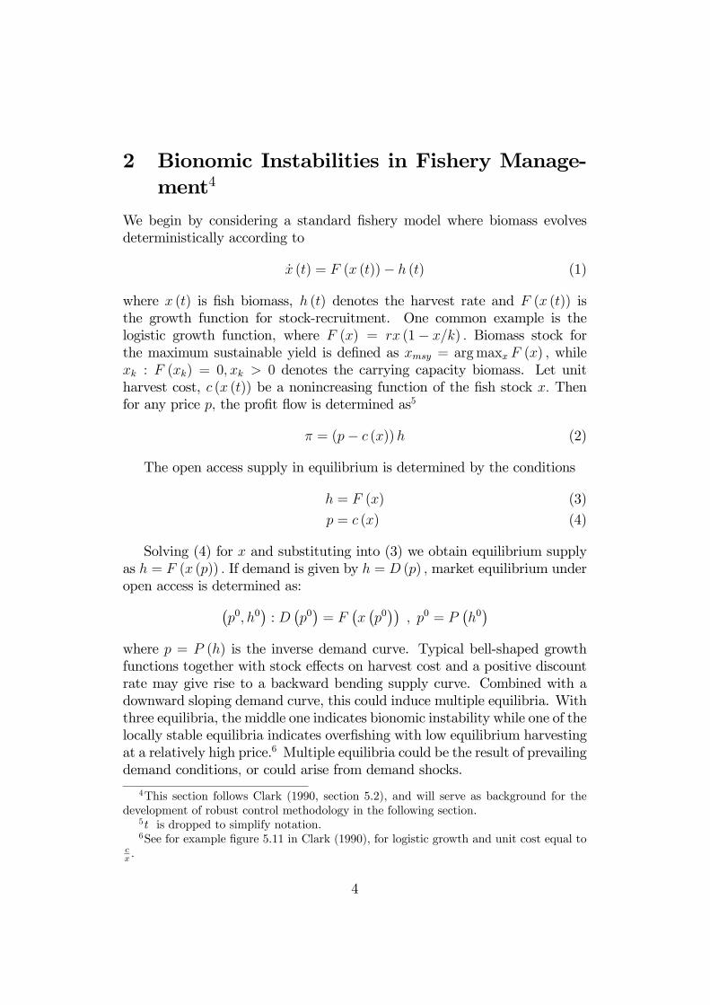
where x (t) is fish biomass, h (t) denotes the harvest rate and F (x (t)) isthe growth function for stock-recruitment. One common example is thelogistic growth function, where F (x) = rx (1− x/k) . Biomass stock forthe maximum sustainable yield is defined as xmsy = argmaxx F (x) , whilexk : F (xk) = 0, xk > 0 denotes the carrying capacity biomass. Let unitharvest cost, c (x (t)) be a nonincreasing function of the fish stock x. Thenfor any price p, the profit flow is determined as5

π = (p− c (x))h (2)

The open access supply in equilibrium is determined by the conditions

h = F (x) (3)

p = c (x) (4)

Solving (4) for x and substituting into (3) we obtain equilibrium supplyas h = F (x (p)) . If demand is given by h = D (p) , market equilibrium underopen access is determined as:¡

p0, h0¢: D

¡p0¢= F

¡x¡p0¢¢

, p0 = P¡h0¢

where p = P (h) is the inverse demand curve. Typical bell-shaped growthfunctions together with stock effects on harvest cost and a positive discountrate may give rise to a backward bending supply curve. Combined with adownward sloping demand curve, this could induce multiple equilibria. Withthree equilibria, the middle one indicates bionomic instability while one of thelocally stable equilibria indicates overfishing with low equilibrium harvestingat a relatively high price.6 Multiple equilibria could be the result of prevailingdemand conditions, or could arise from demand shocks.

4This section follows Clark (1990, section 5.2), and will serve as background for thedevelopment of robust control methodology in the following section.

5t is dropped to simplify notation.6See for example figure 5.11 in Clark (1990), for logistic growth and unit cost equal to

cx .

4

To analyze socially optimal fishery management we introduce a socialplanner or a regulator maximizing net surplus defined as U (h) − c (x)h,

where U (h) =R h0P (u) du so that U 0 (h) = P (h) . The welfare maximization

problem is defined as:

maxh(t)

Z ∞

0

e−ρt [U (h (t))− c (x (t))h (t)] dt (5)

s.t. x (t) = F (x (t))− h (t) , x (0) = x0 > 0 (6)

The current value Hamiltonian for the problem is:

H = U (h)− c (x)h+ λ [F (x)− h] (7)

with optimality conditions

U 0 (h) = λ+ c (x) , U 0 (h) = P (h) (8)

λ = [ρ− F 0 (x)]λ+ c0 (x)h (9)

along with biomass evolution (6) and the transversality condition at infinity.Differentiating (8) with respect to time and substituting into (9) we obtainthe dynamic system that characterizes the optimal paths of harvest and fishstock. The behavior of harvest is given by

h =1

U 00 (h)[(ρ− F 0 (x)) (U 0 (h)− c(x)) + c0 (x)F (x) , U 0 (h) = P (h)]

(10)whereas stock behaves according to (6). The deterministic steady state equi-librium is defined as h = x = 0. At the steady state, market equilibrium ischaracterized by

P (h) = p, p = c (x)− c0 (x)F (x)ρ− F 0 (x)

= Sρ (x) , h = F (x) (11)

which describe demand, supply, and biological equilibrium respectively. Solv-ing the stock equilibrium equation of (11), market equilibrium when the fish-ery is optimally managed is defined as

(p∗, h∗) : P (h∗) = Sρ (x (h∗)) , p∗ = P (h∗) (12)

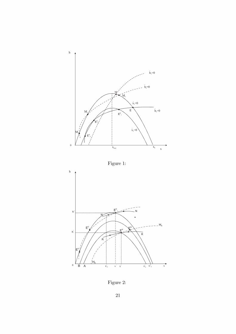
The discounted supply curve determined by (11) is backward bending asin the case of open access fishery and could induce multiple equilibria, aspresented in the phase diagram of figure 1.7

7See also Clark (1990) figures 5.17 and 6.12.

5

[Figure 1]

For the h1 = 0 isocline there is a unique steady state which is saddle pointstable atM . However, a demand shock could shift this isocline to hs = 0 andinduce multiple equilibria, atM1, M2, andM3, with the middle one being un-stable and M3 indicating overfishing. Furthermore, if the benchmark modelfor stock evolution is misspecified, it is possible for a worse than estimatedmodel for the stock-recruitment relationship F (x) to be realized. Under de-mand shocks and misspecification of the stock-recruitment relationship boththe x = 0 isocline and the h = 0 isocline shift and multiple equilibria couldalso be induced. If these shifts yield a system such as x2 = 0, h2 = 0 thenmultiple equilibria emerge at ED

1 , ED2 , E

D3 . It is also possible for the true

model to correspond to an x = 0 isocline even further below x2 = 0, so thatan equilibrium with harvesting rule h2 = 0 does not exist. This harvestingrule would lead to resource collapse under such circumstances.The possibility of multiple equilibria at the social optimum presents prob-

lems for regulation. For example, the regulatory instruments could have beendesigned to steer the system towards M1 but due to demand shocks and/ormisspecification, as described above, the systems could converge, for appro-priate initial conditions, to a state like ED

3 which is an overfishing steadystate. To prevent regulatory complications arising from such cases a dif-ferent type of regulation is required. The idea behind the robust controlmethodology, as applied in this paper to fishery management, is to help de-sign rules which under the worst possible scenario for the stock-recruitmentrelationship will prevent instabilities, steady state multiple equilibria andbiological overfishing.

3 Robust Control and Fishery Management

To develop the robust control methodology we introduce uncertainty in thestock-recruitment equation. Let (Ω,F ,G) be a complete probability space,and let xt = x (ω, t) , ht = h (ω, t) be the stochastic processes for the fishbiomass and harvesting, respectively. Moreover, letBt = B (ω, t) be aWienerprocess, E (dBt) = 0, var (dBt) = dt.The stochastic social optimization problem for the fishery can be defined

as the choice of a nonanticipating harvesting process h (ω, t) that maximizesthe expected value of net surplus, subject to the constraints imposed by

6

species growth rate:8

maxh(t)

E0Z ∞

0

e−ρt [U (ht)− c (xt)ht] dt (13)

s.t. dx (t) = [F (xt)− ht] dt+ σdBt (14)

σ > 0, x (0) = x0 > 0 nonrandom (15)

xt ≥ 0, ht ≥ 0 (16)

where xt is the state variable and ht is the control variable of the stochasticcontrol problem.In equation (14) the term F (xt) − ht represents the expected change

in the fish biomass at any given point in time, while the term σdBt is therandom amount of biomass change, with zero mean and variance σ2. In thissetup, which is a typical stochastic control problem, the manager is assumedto know the behavior of stochastic shocks well enough to fully trust thecharacterization of the probability distribution implied by (14). This basicassumption leads to a decision on optimal harvest paths. However, it is quitepossible (indeed likely, given natural system characteristics and informationgaps) that the distribution is only an estimate, so that there is a degree ofuncertainty attached not just to the specific realization of the random shockbut also to the distribution itself. In other words, the planner might want toconsider his own doubts about the model he is using to represent randomness.9

Following Hansen et al. (2002), we regard (14) as a benchmark model. Ifwe assume that the social planner knows the benchmark model then thereare no concerns about robustness to model misspesification. Otherwise, theseconcerns for robustness to model misspecification are reflected by a family ofstochastic perturbations to the Brownian motion Bt : t ≥ 0 . The pertur-bation distorts the probabilities G implied by (14) and replaces G by anotherprobability measure Q. The main idea is that stochastic processes under Qwill be difficult to distinguish from G using a finite amount of data. Theperturbed model is constructed by replacing Bt in (14) with

Bt = zt +

Z t

0

Rsds, or dBt = dzt +Rtdt (17)

where zt : t ≥ 0 is a Brownian motion and Rt : t ≥ 0 is a measurabledrift distortion. Changes in the distribution of Bt will be parametrized as

8The basic assumption is that species biomass fluctuates continuously and that thesestochastic influences are adequately represented by Wiener processes.

9There are two essentially different types of uncertainty involved. Chevé and Congar(2000) refer to these as risk (not knowing the precise value the shock will take) andimprecision (not being sure of the model).

7

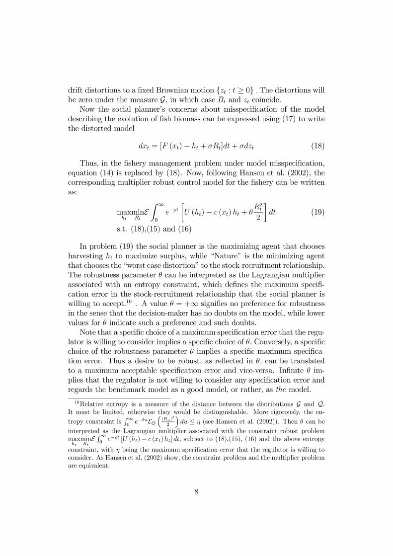
drift distortions to a fixed Brownian motion zt : t ≥ 0 . The distortions willbe zero under the measure G, in which case Bt and zt coincide.Now the social planner’s concerns about misspecification of the model

describing the evolution of fish biomass can be expressed using (17) to writethe distorted model

dxt = [F (xt)− ht + σRt]dt+ σdzt (18)

Thus, in the fishery management problem under model misspecification,equation (14) is replaced by (18). Now, following Hansen et al. (2002), thecorresponding multiplier robust control model for the fishery can be writtenas:

maxhtminRt

EZ ∞

0

e−ρt·U (ht)− c (xt)ht + θ

R2t2

¸dt (19)

s.t. (18),(15) and (16)

In problem (19) the social planner is the maximizing agent that choosesharvesting ht to maximize surplus, while “Nature” is the minimizing agentthat chooses the “worst case distortion” to the stock-recruitment relationship.The robustness parameter θ can be interpreted as the Lagrangian multiplierassociated with an entropy constraint, which defines the maximum specifi-cation error in the stock-recruitment relationship that the social planner iswilling to accept.10 . A value θ = +∞ signifies no preference for robustnessin the sense that the decision-maker has no doubts on the model, while lowervalues for θ indicate such a preference and such doubts.Note that a specific choice of a maximum specification error that the regu-

lator is willing to consider implies a specific choice of θ. Conversely, a specificchoice of the robustness parameter θ implies a specific maximum specifica-tion error. Thus a desire to be robust, as reflected in θ, can be translatedto a maximum acceptable specification error and vice-versa. Infinite θ im-plies that the regulator is not willing to consider any specification error andregards the benchmark model as a good model, or rather, as the model.

10Relative entropy is a measure of the distance between the distributions G and Q.It must be limited, otherwise they would be distinguishable. More rigorously, the en-

tropy constraint isR∞0

e−δuEQ³|Ru|22

´du ≤ η (see Hansen et al. (2002)). Then θ can be

interpreted as the Lagrangian multiplier associated with the constraint robust problemmaxhtminRtE R∞

0e−ρt [U (ht)− c (xt)ht] dt, subject to (18),(15), (16) and the above entropy

constraint, with η being the maximum specification error that the regulator is willing toconsider. As Hansen et al. (2002) show, the constraint problem and the multiplier problemare equivalent.

8

Using the Fleming and Souganidis (1989) result on the existence of arecursive solution to the multiplier problem, Hansen et al. (2002) show thatproblem (19) can be transformed into a stochastic infinite horizon two-playergame where the Bellman-Isaacs conditions imply that the value functionJ (xt, θ) satisfies11

ρJ (x, θ) = maxhminR

( hU (h)− c (x)h+ θR

2

2

i+

Jx [F (x)− h+ σR] + 12σ2Jxx

)(20)

= minRmaxh

( hU (h)− c (x)h+ θR

2

2

i+

Jx [F (x)− h+ σR] + 12σ2Jxx

)

A solution for game (20) for any given value of the robustness parameterθ will determine the socially optimal robust harvesting policy.

3.1 Robust harvesting rules

The optimality conditions associated with the optimization in the right handside of (20) imply

U 0 (h)− c (x) = Jx (21)

R = −σθJx (22)

Equation (21) is the usual result that at the optimal harvest the netmarginal benefit of an additional unit of catch must be equal to the resourcecost, whereas equation (22) is the worst possible distortion that is admissible,which is negative as expected and depends on θ. When θ is large, R is smalland the benchmark model is a good approximation. More specifically, whenθ → ∞ there is no distortion at all and the model yields the same solutionas the typical optimal stochastic control model.Going through the required derivations (see Appendix A), we obtain the

solution for the evolution of harvesting (in expected terms), which dependson the distortion R :

(1/dt) Edh = 1

U 00 (h)

½[ρ− F 0 (x)] (U 0 (h)− c (x)) + c0 (x) [F (x) + σR]

+12σ2c00 (x)− 1

2U 000 (h)σ2h2x

¾(23)

substituting the worst case distortion R from first order condition (22), wehave the differential equation governing the change of the expected value of

11t is dropped again to simplify notation.

9

robust harvesting along the optimal path.

(1/dt) Edh = 1

U 00 (h)

" hρ− F 0 (x)− σ2

θc0 (x)

i(U 0 (h)− c (x)) + c0 (x)F (x)

+12σ2 (c00 (x)− U 000 (h)h2x)

#(24)

Likewise, the evolution of the expected value of biomass, after substitutingR from equation (22) into equation (18) and taking expected values, becomes

(1/dt) Edx = F (x)− h− σ2

θ(U 0 (h)− c (x)) (25)

Equations (24) and (25) summarize the evolution of the expected valuesof harvesting and biomass under socially optimal management with robustcontrol.

4 Robust Equilibrium: Uniqueness and Reg-ulation

In equilibrium (1/dt) Edh = (1/dt) Edx = 0. Using (24) and recalling thatU 0 (h) = P (h) , the socially optimal expected steady state harvest underrobust control will be determined by:

ρ = F 0 (x) +σ2

θc0 (x)− c0 (x)F (x) + 1

2σ2 (c00 (x)− U 000 (h)h2x)

P (h)− c (x)(26)

Under certainty σ = 0, in which case (26) is reduced to the well known rulefor optimal fishery management, equation (11). Similarly, the managementrule under “typical”, risk-type uncertainty in stock-recruitment, without apreference for robustness, is obtained by setting σ 6= 0 and θ →∞.Solving (26) for P (h) the robust equilibrium market clearing conditions

become:

p = P (h) =

c (x)−"c0 (x)F (x) + 1

2σ2 (c00 (x)− U 000 (h)h2x)

ρ− F 0 (x)− σ2

θc0 (x)

#(27)

h+σ2

θU 0 (h) = F (x) +

σ2

θc (x) (28)

where condition (28) indicates stationary biomass, xθ(h, θ). Substitutinginto (27) we obtain the robust supply curve p = Sθ (h, θ) . Then marketequilibrium is obtained as:

(p∗θ, h∗θ) : P (h

∗θ) = Sθ (h

∗θ, θ) and p∗θ = P (h∗θ) (29)

10

Setting θ → ∞ we obtain the corresponding equilibrium condition underrisk. It is interesting to note that the simpler type of randomness (assuminga known distribution) affects only the supply curve (??), but not the stockequilibrium condition (??). However, once we allow for model uncertaintythe stock equilibrium condition is also affected by the robustness parameter,so that both harvest and stock expected paths are modified. The chosenequilibrium will depend on σ (which is assumed to be exogenous) as well asθ. Now the interesting question is how to choose an appropriate value forthis parameter. One possibility is to use the detection error probabilitiesassociated with a given sample of observations for biomass evolution, cal-culating likelihood ratios between different worst case distributions and thebenchmark (see Hansen and Sargent (2003)).Alternatively, the discussion in section 2 suggests that the dynamic fishery

model could be associated with problems of multiple equilibria and bionomicinstabilities, which suggests that θ could also be used to eliminate such prob-lems. To make the point clear, assume that the fishery is controlled usingonly the benchmark model (14), which implies that θ → ∞. The dynamicsystem for expected harvesting and biomass is defined, using (23) and (25)for θ→∞, by:

(1/dt) Edh =1

U 00 (h)

½[ρ− F 0 (x)] (U 0 (h)− c (x)) + c0 (x)F (x)

+12σ2c00 (x)− 1

2U 000 (h) σ2h2x

¾(30)

(1/dt) Edx = F (x)− h (31)

Suppose that this system has a unique equilibrium with the usual saddlepoint property, shown, in Figure 1, as the intersection of x1 = 0 and h2 = 0at point E. Assume now that the benchmark model is not the true one, butthat the true one is a distorted model for some RD < 0. Since there are norobust control considerations by the manager, the corresponding dynamicsystem in expected values is given by (30) and

(1/dt) Edx = F (x)− h+RD

In this case while the (1/dt) Edh = 0 isocline remains the same, the (1/dt) Edx =0 isocline shrinks inward, possibly as far as the x2 = 0 isocline in Figure 1,inducing multiple equilibria at ED

1 , ED2 , and ED

3 . If RD is sufficiently large

in absolute value, then there could be no steady state equilibrium at all andthe resource might collapse. Thus controlling with the benchmark modelwhen the distorted model is true could lead to instabilities or even resourcecollapse.12

12These effects will be more profound and detrimental the faster the biomass and harvestdynamics.

11

The idea behind stabilization through robust control is to choose a har-vesting rule such that the system has a unique equilibrium not only for thebenchmark model but for the worst possible distortion R that Nature couldchoose. If a unique equilibrium exists under the worst possible distortion,we want to show that uniqueness will also hold for milder distortions of thebenchmark model.Under robust control the equilibrium harvesting and biomass are deter-

mined by (24), (25). In this system θ can be used as a free parameter.Therefore, it could be chosen in principle so that the system has a uniqueequilibrium. This idea can be explained with the help of Figure 2, which de-picts again the three equilibria that emerge from the distorted model withoutrobust control, ED

1 , ED2 , and ED

3 of Figure 1. Choosing a specific θ impliesthat the (1/dt)Edh = 0 and the (1/dt)Edx = 0 isoclines of the system (24),(25) will shift. The idea is to choose θ so that the isoclines shift to positionssuch as HRHR and AxRk , intersecting only once at point E

R.

[Figure 2]

Choosing θ this way implies that the preference for robustness is combinedwith a preference for uniqueness. A specific value of θ that guarantees aunique, stable equilibrium can be translated to a maximum specificationerror that the manager or regulator is willing to accept, by recalling θ0s role asmultiplier of the entropy constraint in the constraint problem formulation.13

Provided that uniqueness is preserved under milder distortions, the use ofrobust control ensures that a unique equilibrium exists for all distortionsfrom the benchmark case to the worst one. Thus, if a milder distortion shiftsthe (1/dt)Edx = 0 isocline to BxMk in Figure 2, since the robust controlsolution fixes the (1/dt)Edh = 0 isocline at HRHR, uniqueness is preservedat EM .An approach for choosing such a θ can be described as follows. Let

(x, h) ∈ A ⊂ R2+, where A = (0, hmax) ⊗ (0, xmax) , xmax > xk. and hmax

sufficiently large but without violating any technical constraints. Let θ ∈Θ = (θ,∞), where θ defines the lower bound of admissible values of θ, ie.the nonnegative values of θ for which the objective function can be larger than−∞. The (1/dt) Edx = 0 isocline defines, using (25), the curve G (x, h; θ) =0, while the (1/dt) Edh = 0 isocline defines, using (24), the curveK (x, h; θ) =13The uniqueness - stabilization argument used in this paper can be complementary

to the detection error probability approach. For instance, it is possible that more thanone value of θ achieve uniqueness, in which case detection error probabilities can provideadditional input into the final choice.

12

0. If a θ∗ exists such that G (x, h; θ∗) = 0 and K (x, h; θ∗) = 0 have a uniquesolution (x∗, h∗) , then robust control leads to a unique equilibrium. Sufficientconditions for the existence of such a θ can be derived.Consider the Jacobian determinant of the system (24), (25):

D (x, h; θ) =

¯Gx (x, h; θ) Gh (x, h; θ)Kx (x, h; θ) Kh (x, h; θ)

¯for (x, h) ∈ A, θ ∈ Θ ⊆ Θ (32)

where Θ is the subset of values of θ for which the a solution for the systemexists.

Proposition 1 If D (x, h; θ) does not change sign in A ⊗ Θ ⊆ Θ then aunique robust equilibrium exists for the expected values of harvest and bio-mass.

For proof see Appendix B.

A possible illustration of this result can be presented with reference toFigure 2. The uniqueness condition means that a θ∗ is selected such that theHRHR curve cuts the horizontal axis between A and xRk , that it is monotonicincreasing at least up to xRk , and that the intersection takes place at thenon increasing part of the AxRk curve.

14 At the equilibrium point the slopecondition for the HRHR and AxRk curves implies, using (32), that

−Kx (x, h; θ∗)

Kh (x, h; θ∗)

> −Gx (x, h; θ∗)

Gh (x, h; θ∗)or

dh (θ∗)dx

¯(1/dt)Edh=0

>dh (θ∗)dx

¯(1/dt)Edx=0

For D (x, h; θ∗) = GxKh −KxGh < 0 the robust equilibrium has the saddlepoint property.To locate sufficient conditions for uniqueness to be preserved under milder

distortions, consider a θ∗ that provides a unique equilibrium satisfying Propo-sition 1. For this value of θ the triplet (x∗, h∗, θ∗) will determine a corre-sponding R∗ which is the worse possible distortion. Consider now arbitrarydistortions R ∈ [R∗, 0] , with R = 0 corresponding to the benchmark modeland R = R∗ corresponding to the robust model. Thus as R increases towardzero we have milder distortions and the (1/dt) Edx = 0 isocline shifts. Interms of Figure 2 this means that the AxRk curve shifts outwards uniformly.Keep the HRHR to the robust equilibrium position determined by the triplet(x∗, h∗, θ∗) , and consider the sequence of determinants:

D³x, h; R

´=

¯¯ Gx

³x, h; R

´Gh

³x, h; R

´Kx (x

∗, h∗;R∗) Kh (x∗, h∗;R∗)

¯¯ (33)

14An intersection could take place at the increasing part of the AxRk curve, but additionalconditions would be required to ensure uniqueness in that case.

13

It is clear that D (x, h;R∗) = D (x, h; θ∗) .

Proposition 2 If D³x, h; R = 0

´has the same sign as D (x, h; θ∗) and it

is monotonic in R then the uniqueness of the robust equilibrium is preservedunder milder distortions in (R∗, 0]

For proof see Appendix ??.

In terms of Figure 2, uniqueness is obtained if the (1/dt)Edh = 0 isoclineis increasing at least up to the carrying capacity of the benchmark model.Furthermore, since AxRk shifts uniformly outwards, say to Bxmk in figure 2,while HRHR remains fixed, uniqueness with the saddle point property ispreserved up to the benchmark model.15

Of course it is possible that several θ satisfy the sufficient conditionsdescribed above. In such a case, the value for θ can be chosen to ensurethe highest expected value for the robust control problem.16 More formally,among the set of θ that satisfy conditions for uniqueness and preservation ofuniqueness under milder distortions, a θ∗∗ is chosen such that:

θ∗∗ = argmaxθEZ ∞

0

e−ρt"U (h∗t (θ))− c (x∗t (θ))h

∗t (θ) + θ

R∗ (θ)2

2

#dt

where h∗t (θ) , x∗t (θ) , R

∗ (θ) are solutions of the robust control problem eval-uated at each θ.If a unique robust equilibrium is defined, the value obtained for harvest-

ing in these conditions can be used as a robust quantity limit for designingtradable quota systems. In this case a robust quota is determined by a policyfunction hRt = φ (xt) which is the function characterizing an approach pathto the unique robust equilibrium. This is the path RR corresponding tothe one dimensional stable manifold of the saddle point robust equilibrium,converging to ER in Figure 2.17 This result can be related to the safe quota15If milder distortions are realized, updates of the policy might be possible. The analysis

of the updating process for a robust rule is left for future research.16Given empirical data, the set of allowable θ can be narrowed down to those that

generate reasonable detection error probabilities. See footnote 13.17The stable manifold or equivalently the policy function hRt = φ (xt) can be recovered by

numerical methods. Using the time elimination method, the stable manifold is determinedby the solution of the differential equation

dh

dx=(1/dt)Edh(1/dt)Edx

with initial conditions (x∗, h∗) , which is the robust steady state corresponding to ER inFigure 2.

14

concept discussed in Homans and E.Wilen (1997). They assume a quota thatis a linear function of the biomass, so that the safe quota is determined ashS = max 0, c+ dx , with c < 0, d > 0. Thus if the stock is below someminimum value then hS = 0 (as negative harvesting is obviously ruled out),while the quota is below, equal or above biological growth if x T xsafe, re-spectively. In our case for each stock level the quota is "safe" in the sensethat it ensures that the robust equilibrium biomass is attained in the longrun even under the worst possible scenario for stock-recruitment.It should be noted that the robust quota rule which attains a steady

state biomass equilibrium for the worst possible case of the stock-recruitmentequation implies smaller harvesting relative to the benchmark model. If thebenchmark model was actually the true model, then with initial condition xR0in Figure 2, the benchmark quota would be determined by the stable manifoldNN converging to ED

1 , which defines the policy function hNt = ψ (xt) . Thedifference hNt −hRt can be interpreted as the reduction in harvesting inducedby the decision to follow robust rules. Moreover, the difference

1

ρE ©[U (h∗)− c (h∗, x∗)]− £U ¡h+¢− c

¡h+, x+

¢¤ªwill indicate the change in expected steady state welfare between robust andbenchmark rules. Since this difference is negative, it can be interpreted asthe steady state cost of wanting to be robust, or to put it in a different way,as the cost of precaution.

5 Concluding Remarks

Bionomic instability is an inherent characteristic of fishery models inducedby a backward bending supply curve. This instability emerges both in openaccess and in optimally controlled fisheries. Given the uncertainties associ-ated with fisheries, these instabilities could be intensified by demand shocksor uncertainties associated with the stock-recruitment relationship.In the present paper we consider the case of scientific uncertainty in the

stock-recruitment relationship and we introduce robust control methods infishery management. We show that robust control could act as a tool toprevent instabilities, by an appropriate choice of the robustness parameter.This is obtained by designing a rule so that the optimally managed fisheryis stable under a worst possible scenario for the stock-recruitment relation-ship.The robust management rule can be used to design a robust quota rulethat work better than typical prescriptions under uncertainty, both in thesense of maintaining stable harvests and in avoiding biomass collapse. This

15

management rule will, however, have a cost in terms of foregone expectedharvesting benefits.The robust harvesting solution can be used as a basis for setting "safe"

quotas to be applied in a fishery. The question of whether and when itmakes sense to update the robustness parameter as more information be-comes available on stock-recruitment, and thus to update the harvesting ruleaccordingly, is one potencially important question which should be addressedin future research.Finally, the basic model developed here can also be extended along dif-

ferent lines, such as depensation or non-linear cost effects, or by consideringthe fishery as a dynamic game between the planner/regulator and the fish-ermen, and seeking robust solutions with possible heterogenous preferencesfor robustness.

16

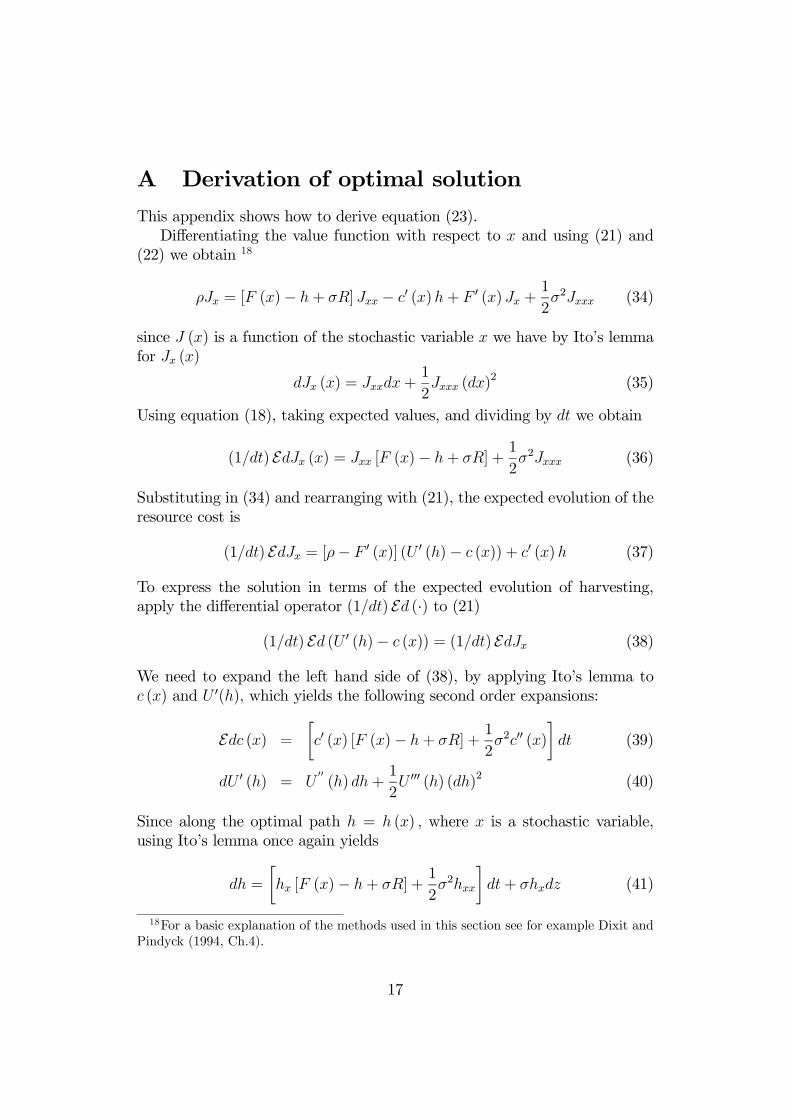
A Derivation of optimal solution

This appendix shows how to derive equation (23).Differentiating the value function with respect to x and using (21) and

(22) we obtain 18

ρJx = [F (x)− h+ σR]Jxx − c0 (x)h+ F 0 (x)Jx +1

2σ2Jxxx (34)

since J (x) is a function of the stochastic variable x we have by Ito’s lemmafor Jx (x)

dJx (x) = Jxxdx+1

2Jxxx (dx)

2 (35)

Using equation (18), taking expected values, and dividing by dt we obtain

(1/dt) EdJx (x) = Jxx [F (x)− h+ σR] +1

2σ2Jxxx (36)

Substituting in (34) and rearranging with (21), the expected evolution of theresource cost is

(1/dt) EdJx = [ρ− F 0 (x)] (U 0 (h)− c (x)) + c0 (x)h (37)

To express the solution in terms of the expected evolution of harvesting,apply the differential operator (1/dt) Ed (·) to (21)

(1/dt) Ed (U 0 (h)− c (x)) = (1/dt) EdJx (38)

We need to expand the left hand side of (38), by applying Ito’s lemma toc (x) and U 0(h), which yields the following second order expansions:

Edc (x) =

·c0 (x) [F (x)− h+ σR] +

1

2σ2c00 (x)

¸dt (39)

dU 0 (h) = U00(h) dh+

1

2U 000 (h) (dh)2 (40)

Since along the optimal path h = h (x) , where x is a stochastic variable,using Ito’s lemma once again yields

dh =

·hx [F (x)− h+ σR] +

1

2σ2hxx

¸dt+ σhxdz (41)

18For a basic explanation of the methods used in this section see for example Dixit andPindyck (1994, Ch.4).

17

When taking the expected value, terms of order higher than t go to zero, sothat E (dh)2 = σ2h2xdt, and (40) becomes

EdU 0 (h) = U00(h) Edh+ 1

2U 000 (h)σ2h2xdt (42)

Using equations (39) and (42) to plug into (38), and recalling (37) we finallyobtain

(1/dt) Edh = 1

U 00 (h)

½[ρ− F 0 (x)] (U 0 (h)− c (x)) + c0 (x) [F (x) + σR]

+12σ2c00 (x)− 1

2U 000 (h)σ2h2x

¾.

(43)

B Proof of Proposition 1

We locate sufficient conditions for the existence of a

The proof follows from the proof of proposition 1. All the D³x, h; R

´deter-

minants are different than zero and do not change sign. Then the implicitvalue theorem and the index theorem provide existence and uniqueness undermilder distortions. ¥

18

References

0 .2 .Androkovich, R. A. and K.R.Stollery (1989), ‘Regulation of stochastic fish-eries: A comparison of alternative methods in the pacific halibut fishery’,Marine Resource Economics 6, 109—122.

Chevé, M. and Congar, R. (2000), ‘Optimal pollution control under impreciseenvironmental risk and irreversibility’, Risk Decision and Policy 5, 151—164.

Chevé, M. and Congar, R. (forthcoming), ‘La gestion des risques environ-mentaux en présence d’incertitudes et de controverses scientifiques: Uneinterprétation du principe de précaution’, Revue Économique .

Clark, C. W. (1990),Mathematical Bioeconomics: The Optimal Managementof Renewable Resources, John Wiley Sons Inc.

Conrad, J. M. (2000), Resource Economics, Cambridge University Press.

Conrad, J. M. and Clark, C. W. (1988), Natural Resource Economics: Notesand Problems, Cambridge University Press.

Danielson, A. (2002), ‘Efficiency of catch and effort quotas in the presence ofrisk’, Journal of Environmental Economics and Management 43, 20—33.

Dixit, A. K. and Pindyck, R. S. (1994), Investment under Uncertainty,Princeton University Press, Princeton, New Jersey.

Fleming, W. H. and Souganidis, P. E. (1989), ‘On the existence of valuefunctions of two-player, zero sum stochastic differential games’, IndianaUniversity Mathematics Journal pp. 293—314.

Gilboa, I. and Schmeidler, D. (1989), ‘Maximin expected utility with non-unique prior’, Journal of Mathematical Economics 18, 141—153.

Hansen, L. and Sargent, T. (2001), ‘Acknowledging misspecification inmacroeconomic theory’, on the Web.URL: ftp://zia.stanford.edu/pub/sargent/webdocs/research/costa6.pdf

Hansen, L. and Sargent, T. (2003), ‘Robust control and model uncertaintyin macroeconomics’, on the Web.URL: ftp://zia.stanford.edu/pub/sargent/webdocs/research/rgamesb.pdf

Hansen, L. et al. (2002), ‘Robustness and uncertainty aversion’, on the Web.URL: http://home.uchicago.edu/ lhansen/uncert12.pdf

19

Homans, F. R. and E.Wilen, J. (1997), ‘A model of regulated open accessresource use’, Journal of Environmental Economics and Management32, 1—21.

Mas-Colell, A., Whinston, M. D. and Green, J. R. (1995), MicroeconomicTheory, Oxford University Press.

McDonald, A. and Hanf, G.-H. (1992), ‘Bio-economic stability of the northsea shrimp stock with endogenous fishing effort’, Journal of Environ-mental Economics and Management 22, 38—56.

Milnor, J. (1965), Topology from the Differentiable Viewpoint, The UniversityPress of Virginia.

Roseta-Palma, C. and Xepapadeas, A. (forthcoming), ‘Robust control in wa-ter management’, Journal of Risk and Uncertainty .

Tu, P. and Wilman, E. (1992), ‘A generalized predator-prey model: Un-certainty and management’, Journal of Environmental Economics andManagement 23, 123—138.

Weitzman, M. (2002), ‘Landing fees vs harvest quotas with uncertain fishstock’, Journal of Environmental Economics and Management 43, 325—338.

Woodward, R. and Bishop, R. (1997), ‘How to decide when experts dis-agree: Uncertainty-based choice rules in environmental policy’, LandEconomics 73, 492—507.

20

M1

M2

M3

x

h

h =01

h =0s

h =02

x =01

x =02

.

.

.

.

.

xmsy xk

ED1

ED2

ED3

E

0

M

Figure 1:

h

ED1

ED2

ED3

ER EMHR

HR

AB xrk xmk xxr0 x*

R

R

h+

h*

NN

0 x+

Figure 2:

21