J. Earth Syst. Sci. (2019) 128:31 c© Indian Academy of Scienceshttps://doi.org/10.1007/s12040-018-1060-y

INSAT-3D low-level atmospheric motion vectors:Capability to capture Indian summer monsoonintra-seasonal variability

Dineshkumar K Sankhala1,2,*, Sanjib K Deb1 and V Sathiyamoorthy1

1Space Applications Centre, Indian Space Research Organization, Ahmedabad 380 015, India.2Department of Mathematics, Gujarat University, Ahmedabad 380 009, India.*Corresponding author. e-mail: dksankhala90@gmail.com, dksankhaln90@sac.isro.gov.in

MS received 20 July 2017; revised 27 March 2018; accepted 8 May 2018;published online 22 January 2019

In India, Atmospheric Motion Vectors (AMVs) are derived operationally from the advanced Indianmeteorological geostationary satellite INSAT-3D since July 2013 over Indian Ocean region and are usedin the numerical model for forecast improvement. In this study, first-time the low-level monsoon windsderived from INSAT-3D satellite have been used to see how these winds are successful in capturingthe intra-seasonal variability over the Indian Ocean region for the year 2016. A validation of AMVsis done on regular basis. In this study, the validation of low-level AMVs with National Center forEnvironmental Prediction (NCEP) analysis winds carried out during June to September 2016. Theobserved mean monthly features of the Indian Summer Monsoon (ISM) in July and August 2016from low-level AMVs from INSAT-3D match well with those of NCEP analysis winds. INSAT-3Dlow-level AMVs are quite successful in capturing the northward propagation of low level jet andtheir locations during active and break monsoon conditions which are known features of the ISM.They are also able to explain the two dominant modes of variability: (i) one with a periodicitybetween 32 and 64 days, and (ii) another with a periodicity between 8 and 16 days, for the monsoonseason of 2016 when Morlet wavelet transform analysis is performed for time series analysis. An EOFanalysis is performed for the study of the spatial structure of intra-seasonal variability and temporalvariability of INSAT-3D low-level AMVs over the Indian Ocean region for ISM 2016 and quantifies theresults of EOF analysis by performing RMSE analysis between EOFs of INSAT-3D and NCEP winddata.

Keywords. Monsoon; INSAT-3D AMVs; Indian Ocean; EOF analysis.

1. Introduction

The operational derivation of Atmospheric MotionVectors (AMVs) by considering the movementof cloud and water vapour tracers in successiveimages of geostationary satellites (Schmetz et al.1993; Nieman et al. 1997; Velden et al. 1997;

Shimoji and Hayashi 2012) are considered as oneof the most reliable source of wind informationwith higher spatial-temporal coverage over theocean as well as land regions. In India, initiallythe AMVs were retrieved operationally using theimages from Kalpana-1 (Kishtawal et al. 2009)and later many upgradations (i) improvement in

1

0123456789().,--: vol V

31 Page 2 of 12 J. Earth Syst. Sci. (2019) 128:31

height assignment, (ii) improvement in qualitycontrol technique, and (iii) derivation of low-levelwinds using visible and mid-infrared channel, weremade in the operational AMV retrieval algorithmwhen advanced meteorological satellite INSAT-3D was launched during July 2013 (Kaur et al.2013; Deb et al. 2016). The AMVs is one of theimportant inputs to the global and regional assim-ilation systems for the improvement of NumericalWeather Prediction (NWP). The role of AMVs isparticularly significant over the oceans and highlatitudes where in-situ observations are scarce. Theimportance of AMV observations increases par-ticularly over the tropics, where the geostrophiccoupling between the mass and the flow fieldsis weaker in comparison to higher latitudes. Inthe tropical atmospheric processes, the significantimprovement is observed in the weather forecast(Kelly et al. 2004; Bedka and Mecikalski 2005; Debet al. 2010; Kumar et al. 2016) when AMVs isassimilated in both regional and global models.The vertical coverage of AMVs spreads throughhigh to low-levels as per the channel used duringretrieval, viz., AMV retrieved using: (i) infraredchannel data covers entire ranges of atmosphere,i.e., from 100–950 hPa, (ii) water vapour chan-nel data covers only high-level, i.e., from 100–500hPa, while (iii) visible and mid-infrared channeldata covers low-levels, i.e., from 600–950 hPa,respectively. The low-level analyzed winds fromthe different operational numerical models andOceansat-2 scatterometer (OSCAT) surface winds(Sathiyamoorthy et al. 2012) were used to explorethe characteristic behaviour of the Indian Sum-mer Monsoon (ISM). Apart from numerical modelwind other parameters, viz., convection, rainfall(Webster et al. 1998; Goswami and Ajaya Mohan2001; Joseph and Sijikumar 2004) and humid-ity, etc., are used to explain the intra-seasonalvariability of ISM; however, no-one has demon-strated the capabilities of low-level AMVs forcapturing the intra-seasonal variability of ISM.In this study, an attempt has been made todemonstrate the capabilities of low-level AMVs(i.e., 700–950 hPa region) by studying the char-acteristics of the ISM for the year 2016. Thefollowing section 2 briefly summarizes the infor-mation about INSAT-3D level-2 data and detailsabout AMVs derived using different spectral chan-nel data and National Centre for Environmen-tal Prediction (NCEP) numerical model analysisdata. In section 3, the results from the analysisare discussed with different perspectives. Finally,

section 4 summarizes the conclusions from thisstudy.

2. Data used

2.1 INSAT-3D AMVs

The advanced Indian meteorological geostation-ary satellites INSAT-3D is placed at 82◦E overthe Indian Ocean region. It carries a six channelimager for the purpose of enhanced meteorolog-ical research and operational needs. The imagerhas 6 spectral channels and these are: (i) Visible(VIS) for [0.55–0.75 µm], (ii) Short-wave infrared(SWIR) for [1.55–1.70 µm], (iii) Mid-wave infrared(MIR) for [3.8–4.0 µm], (iv) Water vapor (WV)for [6.5–7.1 µm], and (v) two split-window ther-mal infrared (TIR1 and TIR2) for [10.2–11.3 µm]and [11.5–12.5 µm] ranges of spectrum, respec-tively. For the operational retrieval of AMVs, datafrom the VIS, MIR, WV and TIR1 re-sampled at4 km spatial resolution with a coverage area [30◦–130◦E, 50◦S–50◦N] over the Indian Ocean regionare used. The retrieval process is done at eachacquisition, i.e., at every 30 min interval with samecoverage area. The operational INSAT-3D AMVsare received and archived at satellite data archivalcentre at Space Applications Centre, Ahmedabad(https://www.mosdac.gov.in) and IMD Delhi foroperation use in the models. For the present study,operational low-level AMVs retrieved using visible(VIS) and mid-infrared (MIR) channel of INSAT-3D data from 01 June 2016 to 30 September 2016are used. The visible AMVs are retrieved duringday, while MIR AMVs are retrieved during night.The following steps: (i) tracer selection, (ii) tracerheight assignment, (iii) tracking of tracer in thesubsequent images, and (iv) wind buffer generationand quality controls, are followed for the opera-tional derivation of low-level AMVs from visible(VIS) and mid-infrared (MIR) channel of INSAT-3D. The descriptions of each step are presented inDeb et al. (2016).

2.2 NCEP analysis data

The National Center for Environmental Prediction(NCEP) analysis wind data are available (http://nomads.ncdc.noaa.gov/) at 0.5◦ latitude × 0.5◦

longitude resolution globally with 47 vertical pres-sure levels at every 6 hr interval (i.e., 4 times daily).The 6 hr model analysis winds from 01 June 2016to 30 September 2016 are used for this study and

J. Earth Syst. Sci. (2019) 128:31 Page 3 of 12 31

out of 47 vertical pressure levels, 12 (700–950 hPalow) vertical pressure levels are used for this study.Here, 0.5◦ latitude × 0.5◦ longitude resolution dataconverted to 1◦ latitude × 1◦ longitude resolutionfor the verification.

3. Results and discussions

3.1 Preliminary validation

In this section, the quality of INSAT-3D AMVsare assessed with respect to NCEP analysis windsover the Indian Ocean region. Since AMVs areavailable at very coarser resolution (at around110×110 km horizontal resolution) with scatteredmanner, before starting the assessment analysis,daily composite AMVs are generated from theavailable 30 min AMVs. Both VIS AMVs avail-able during day and MIR AMVs available duringnight are combined together to make the griddeddaily composite. In the daily composite, low-levelVIS and MIR AMVs available in the 700–950 hParegion are averaged to represent a single low-levelAMVs. The averaging reduces the data gap in theAMVs. One possible reason for the data gap isthe absence of appropriate cloud tracers during theretrieval of AMVs over that region. For doing col-location the NCEP analysis available 4 times aday are averaged to make daily averaged value.Again model analysis winds available at differentlevels between 700 and 950 hPa are averaged tomake single low-level winds. Finally, two sets of

daily-averaged gridded low-level winds are used forthis study: (i) INSAT-3D AMVs and (ii) NCEPwind analysis over region 30◦–110◦E and 30◦N–30◦S. Figure 1(a and b) shows density scatter plotsbetween INSAT-3D low-level AMVs and NCEPanalysis wind speeds and wind directions. The biasand root mean square error (RMSE) are calcu-lated for wind speed and wind direction is alsoshown in the figure. It is found that the INSAT-3D AMVs wind speed RMSE is around 3.2 ms−1,while that for wind direction is 20◦, respectivelyfor the period of analysis. These values are similarto the values of other AMVs available from dif-ferent other satellites over this region (Deb et al.2016).

3.2 Monthly mean features

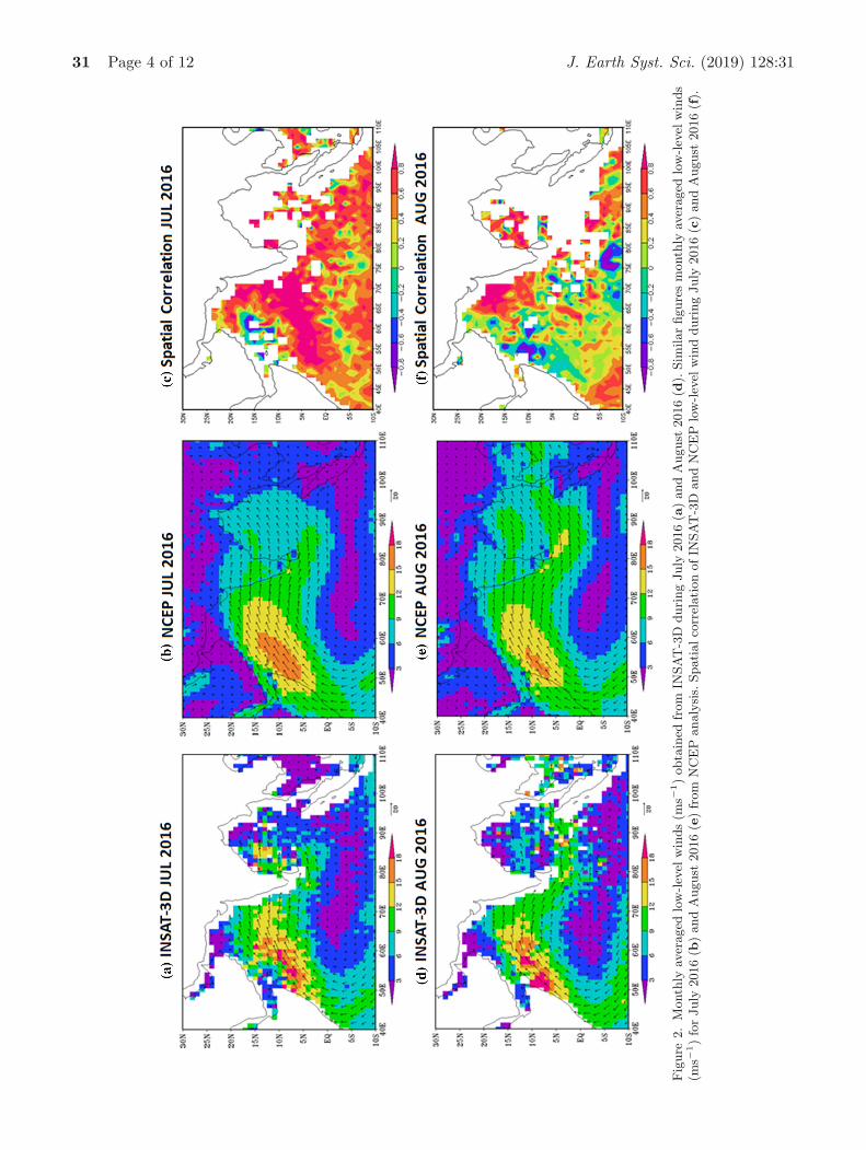
Figure 2(a and d) shows the monthly meanlow-level AMVs from INSAT-3D and figure 2(band e) shows the similar low-level winds fromNCEP reanalysis for the summer monsoon monthsof July and August 2016, respectively. Though,the resolution of INSAT-3D AMVs is coarse, itis quite successful in capturing the important fea-tures of the IMS circulation. From the figures it isnoticed that AMVs are able to capture: (i) cross-equatorial flow of winds along the East Africancoast, (ii) lower level jet (LLJ) over the ArabianSea, (iii) comparatively calm winds near equa-tor on either side, and (iv) southern hemisphericeasterly trade winds. The strength of LLJ is almost

Figure 1. Density scatter plot between INSAT-3D and NCEP analysis (a) wind speed and (b) wind direction during Juneto September 2016. The bias, SD and RMSE are also provided in the figure.

31 Page 4 of 12 J. Earth Syst. Sci. (2019) 128:31

Fig

ure

2.

Month

lyav

eraged

low

-lev

elw

inds

(ms−

1)

obta

ined

from

INSA

T-3

Dduri

ng

July

2016

(a)

and

August

2016

(d).

Sim

ilar

figure

sm

onth

lyav

eraged

low

-lev

elw

inds

(ms−

1)

for

July

2016

(b)

and

August

2016

(e)

from

NC

EP

analy

sis.

Spati

alco

rrel

ati

on

ofIN

SA

T-3

Dand

NC

EP

low

-lev

elw

ind

duri

ng

July

2016

(c)

and

August

2016

(f).

J. Earth Syst. Sci. (2019) 128:31 Page 5 of 12 31

similar in both July and August 2016. Figure 2(cand f) shows the spatial correlation of INSAT-3Dlow-level AMVs and NCEP low-level wind data ofJuly and August 2016, respectively. It is seen fromthe figure that wind speed spatial distribution andits monthly variation INSAT-3D low-level AMVsduring summer monsoon months matches closelywith that of NCEP analysis, indicates the useful-ness of INSAT-3D low-level AMVs for this kind ofstudies.

3.3 Intra-seasonal variability

Many studies (Sikka and Gadgil 1980; Zeng andWang 2009) have revealed that the IMS rain-fall activity has strong intra-seasonal variability intime scale of 30–60 days in the form of active andlull days, which is linked closely with intra-seasonalvariability of the Inter-Tropical Convergence Zone(ITCZ). The ITCZ repeatedly propagates north-ward on intra-seasonal time scales from equatorialIndian Ocean to the monsoon trough region situ-ated over the Indo-Gangetic areas during summermonsoon. This northward propagation is promi-nently active over the Bay of Bengal and adjoininglongitudinal area between 70◦ and 100◦E. Thestudy of Joseph and Sijikumar (2004) reveals thatwhen monsoon is active, the rainfall activity andstrength of the LLJ increase and the axis of LLJ islocated near 15◦N, while during lull days, rainfallactivity and strength of the LLJ decreases and thejet axis is found south of Sri Lanka.

AMVs are available at different heights in scat-tered manner in the places where valid tracersare available. To reduce the data gap to a certainextent, daily composite mean of low-level INSAT-3D AMVs are generated from the coarser 30 mindata. To study the characteristics of intra-seasonalvariability during the 2016 summer monsoon sea-son, daily low-level AMVs are averaged over thecentral part of Bay of Bengal covering the area 80◦–95◦E; 10◦–20◦N, and a time series is presented infigure 3. The central part of Bay of Bengal is chosenbecause intra-seasonal variability is quite promi-nent over the Bay of Bengal and also low-level VISand MIR AMVs available over the oceanic regionto avoid land/coast contamination. Some discon-tinuities in the time series is noticed because ofmissing data for these dates. It is seen from thisfigure that the INSAT-3D low-level winds fluctu-ated a few times during the monsoon season. Thestronger (>10 ms−1) AMVs are noticed during fouroccasions: (i) 08 June 2016, (ii) 30 June 2016,

(iii) 01 August 2016 and (iv) 17 August 2016 andweaker (<6 ms−1) during four occasions: (i) 20June 2016, (ii) 25 July 2016, (iii) 22 August 2016and (iv) 19 September 2016.

The multi-frequency non-stationary powerspresent in a time series can be determined by usingWavelet Transform (Lau and Weng 1995). Thecomplex Morlet wavelet has the capability to detecttime-dependent amplitude and phase for differentfrequencies present in a time series. In this study,a complex Morlet wavelet transform (WT) is usedto find the multi-scale frequencies embedded in thewind time series shown in figure 3. The data gaps inthe time series are filled using interpolation beforethe wavelet transform is applied. The total numberof data points in the time series is taken as 128 (i.e.,27, from 26 May 2016 to 30 September 2016). Thefigure 4 shows the two-dimensional time-frequencyrepresentation of the wavelet transform, in whichthe x-axis represents the days from 26 May 2016 to30 September 2016, while in the y-axis; the periodsin days are shown. The shades in the figure repre-sent the amplitude of INSAT-3D low-level windsand as expected, two prominent modes of variabil-ity are visible in INSAT-3D AMVs during 2016monsoon season. One with higher wavelengths witha periodicity between 32 and 64 days. This is calledas intra-seasonal (30–60 days) variability and thisvariability is noticed three times in 2016 with aperiod of around 30 days. The repeated northwardpropagation of LLJ is the main cause of this vari-ability. The other with lower wavelengths with aperiodicity between 8 and 16 days. The presence of8–16 days variability in INSAT-3D low-level AMVsis associated with the movement of low pressuresystems and other short-period variability presentover the monsoon region. It is noticed that about 10low pressure areas formed over the Indian monsoonregion during the 2016 monsoon season, of whichone formed in June, one in July, five in August andthree in September (Rao et al. 2017).

3.4 Active and lull monsoon periods

The occurrences of active and lull periods are veryimportant phenomena of any monsoon seasons.Active and lull period are well defined phenomenain literature (Webster et al. 1998; Goswami andAjaya Mohan 2001; Joseph and Sijikumar 2004).Webster et al. (1998) have defined an active andbreak period by using a zonal wind criterion overthe north Bay of Bengal and used a fixed cut-off anomaly (+3 or −3 ms−1) to define active

31 Page 6 of 12 J. Earth Syst. Sci. (2019) 128:31

Figure 3. Time series of daily area averaged (i) INSAT-3D low-level winds (ms−1) over the Bay of Bengal box (10◦–20◦N;80◦–95◦E) during 26 May 2016 to 30 September 2016 and (ii) NCEP zonal wind at 850 hPa in the lat.–long. box (10◦–20◦N;70◦–80◦E). The active and lull phases used for further analysis are also shown in the figure. The discontinuities in the timeseries arise from data gaps.

Figure 4. Morlet wavelet analysis of the INSAT-3D low-level winds (ms−1) averaged over the Bay of Bengal box (10◦–20◦N;80◦–95◦E) during the monsoon season of 2016.

and break conditions. Goswami and Ajaya Mohan(2001) have used similar wind criteria for defin-ing active and break monsoon spells. Joseph and

Sijikumar (2004) have defined an active periodas one in which for each day of the period,the area-averaged zonal wind at 850 hPa in the

J. Earth Syst. Sci. (2019) 128:31 Page 7 of 12 31

latitude–longitude box 10◦–20◦N and 70◦–80◦E in 5days period centred on that day is 15 ms−1 or more.The identification of the active and break days isnot very sensitive to small changes in the positionof the reference point (Webster et al. 1998). In thepresent study, active and break period is calculatedusing INSAT-3D AMVs. The days for which thewind speed averaged over the box (80◦–95◦E and10◦–20◦N) are greater than 10 ms−1 for at least3 consecutive days as considered as active days,while those less than 6 ms−1 for at least 3 consecu-tive days (over the box “80◦ –95◦E and 10◦–20◦N”)are considered as break days. It is seen from thefigure 3 that during 2016, the active period wasduring 8–12 July 2016, while lull period was from24–29 July 2016. To study the characteristics ofINSAT-3D AMVs during active and lull monsoonperiods, AMVs and NCEP analysis are averagedduring the 8–12 July for active period and 24–29

July for lull period. The spatial plots INSAT-3DAMVs (figure 5a and b) and corresponding NCEPwind analysis (figure 5c and d) for active andlull periods are shown in figure 5. Though deepand organized convection is largely absent dur-ing monsoon lull periods, low level cumulus andstratiform clouds do present. The AMV retrievalalgorithm is able to track the movement of low-level potential cloud tracers for the retrieval ofvalid AMVs even during lull-period. Few datagaps are noticed in INSAT-3D AMVs, while com-paring with similar plots of NCEP analysis. Asexpected, both INSAT-3D AMVs and NCEP windsshow the northward propagating nature of low-level jet (LLJ) and its locations during active andlull periods. The weak LLJ is present during lullperiod and the 12 ms−1 wind is confined to asmall area near Somalian region. Both INSAT-3D low-level AMVs and NCEP analysis are weak

Figure 5. Average INSAT-3D low-level wind speed (ms−1, shaded) and wind vectors during (a) lull (24–29 July 2016) and(b) active (8–12 July 2016) phases during the 2016 monsoon season. Similarly from NCEP low-level wind speed (ms−1,shaded) and wind vectors during (c) lull (24–29 July 2016) and (d) active (8–12 July 2016) phases during the 2016 monsoonseason.

31 Page 8 of 12 J. Earth Syst. Sci. (2019) 128:31

(<6 ms−1) over the entire Bay of Bengal. Theaxis of LLJ is located south of Sri Lanka and theweak southern hemispheric cross-equatorial flow isalso noticed (figure 5a and c). During the activeperiod, the stronger LLJ is over the entire Ara-bian Sea, and its axis is located north of 15◦Nover the central Bay of Bengal (figure 5b and d).Thus, it can be summarized here that during theactive time, both INSAT-3D low-level AMVs andNCEP wind analysis are stronger over the Bayof Bengal and the Arabian Sea while during lulltime they are weaker in the same region, and theaxis of LLJ is located north of 15◦N (south ofSri Lanka). The locations of LLJ axis as illus-trated by INSAT-3D low-level AMVs during theactive and lull periods matches well with the loca-tions of LLJ during the active and lull periodsreported in the literature (Joseph and Sijikumar2004).

3.5 The monsoon LLJ over the Bay of Bengal

It is well known fact that the ITCZ and LLJrepeatedly move northward on intra-seasonal timescales during the monsoon season. As discussed inthe earlier section, the signatures of northward-propagating LLJs are noticed close to the surface,while its maximum strength is found at 850 hPalevel height. A Hovmollor (time–latitude plot) dia-gram of the INSAT-3D low-level AMVs averagedbetween 80◦ and 95◦E longitudes is presented toassess its northward propagation (figure 6a). Dueto data gap in INSAT-3D AMVs for better under-standing, a similar figure for NCEP low-level windsis shown in figure 6(b). It is seen from these fig-ures that low-level winds near surface shows anorthward propagation pattern, which is clearlyvisible in NCEP wind analysis, while very poorlydepicted in the INSAT-3D AMVs due to large datagap. In 2016, relatively strong winds propagatednorthward around three times from near-equatoriallatitudes to the northern Bay of Bengal. The firstpropagation started around 16 June 2016, the sec-ond one around 20 July 2016 and the last onearound 16 August 2016.

3.6 The principal components of AMVs

In the earlier section, the intra-seasonal variabilityis explained by spectral analysis of area averagedtime series over Bay of Bengal region. However,the method of principal components analysis oftenreferred to as empirical orthogonal function (EOF)

Figure 6. Hovmoller (time–latitude) plot of (a) INSAT-3Dlow-level wind speed (ms−1) and (b) NCEP low-level windspeed (ms−1) averaged between 80◦ and 95◦E longitudeduring the summer monsoon season of 2016. Wind speedcontours above 6 ms−1 are shown.

analysis, can be utilized effectively to link thespatial and temporal patterns of a data field (David1983). Hence, spatial structure of intra-seasonalvariability and associated variability in time can beextracted by using EOF analysis of wind speed overa larger domain. The EOFs analysis of the INSAT-3D AMVs and NCEP low-level winds are calcu-lated over the Indian Ocean region (30◦N–30◦S,40◦–100◦E). Their time series are also been nor-malized. In the present study, first four dominantEOFs of the daily low-level wind time series areperformed for the intra-seasonal variability of ISM2016 that arises from its inherent oscillations of sys-tems through this region. The first EOF of AMVs(figure 7a) explains only 17% of the total vari-ance, while the second, third and fourth EOFs(figure 7b–d) jointly put together explain 29%

J. Earth Syst. Sci. (2019) 128:31 Page 9 of 12 31

(14, 9 and 6%, respectively) of the total varianceof the low-level wind. Thus, the first four EOFsexplain 46% of the total variance of the low-level wind. Similarly, the EOF of NCEP low-levelwinds is calculated. The first EOF of NCEP wind(figure 7e) explains only 20% of the total vari-ance, while the second, third and fourth EOFs(figure 7f–h) jointly put together explain 29%(15, 8 and 6%, respectively) of the total vari-ance of the NCEP wind. Thus, the first fourEOFs explain 49% of the total variance of theNCEP wind. Though the percentage explanationof EOFs of both INSAT-3D AMV and NCEPwinds are not very different, their patterns are

similar in nature. The corresponding time series offirst four principal components of INSAT-3D low-level wind and NCEP wind are also calculated.In figure 8, PC1 (a), PC2 (b), PC3 (c) and PC4(d) are shown for INSAT-3D AMVs and NCEPwind. The amplitude of the PC1 (figure 8a) gradu-ally increases and peaks during the month of Julyand later decreases during August and Septem-ber which depicts the actual behavior of observedrainfall. The EOF2 maps (figure 7b and f) forINSAT-3D AMVs and NCEP winds are not match-ing, as INSAT-3D AMVs (figure 7b) shows negativecorrelation over Arabian Sea, while the oppositefeatures are observed in the NCEP (figure 7f).

Figure 7. Spatial pattern of the first four EOF modes of INSAT-3D AMV and NCEP low-level winds for ISM 2016.

31 Page 10 of 12 J. Earth Syst. Sci. (2019) 128:31

Figure 7. (Continued.)

This is clearly visible in the time-series ofprincipal components (figure 8b) possesses an oscil-lation of high amplitude. The third EOFs ofINSAT-3D AMVs and NCEP winds present someinteresting results even though they explain muchlower proportion of the variance. EOF3 (figure 7cand g) divide ISM region just into two parts, withnegative correlations over Arabian Sea and pos-itive correlations in the southern Indian Ocean.This clearly shows an east–west intra-seasonalvariation of the summer time circulation. Theamplitude of PC3 (figure 8b) for INSAT-3D andNCEP winds also matches very closely throughoutthe Indian summer monsoon season. The maps of

EOF4 (figure 7d and h) show the contribution ofweather-scale disturbances to intra-seasonal vari-ability. The time series of EOF4 (figure 8d) isapparently composed of rapid oscillations as com-pared to the time series of other EOFs. The RMSEanalysis between EOFs of AMVs and NCEP dataare carried out to quantify the performance ofAMV in capturing spatial and temporal pattern ofintra-seasonal variability. The RMSE of EOF1,EOF2, EOF3 and EOF4 between NCEP andINSAT-3D AMVs are 0.0004, 0.0039, 0.0010 and0.0009, respectively. The corresponding RMSE forPC1, PC2, PC3 and PC4 are 3.07, 35.05, 5.99 and5.88, respectively.

J. Earth Syst. Sci. (2019) 128:31 Page 11 of 12 31

Figure 8. Time series of principal component of the first four modes of INSAT-3D and NCEP low-level wind for ISM 2016.

4. Conclusions

In this study, first time the capabilities of INSAT-3D low-level AMVs are explored to study the ISMintra-seasonal variability as captured by it dur-ing the year 2016. INSAT-3D low-level AMVs arequite successful in capturing all the observed fea-tures of the ISM. When a complex Morlet wavelettransform is used to wind time-series, it showstwo prominent modes of variability one with 32–64 days periodicity and the other with 8–16 daysperiodicity in 2016 in INSAT-3D low-level AMVs.

The rainfall activities over the Indian monsoonregion are significantly due to these two variabil-ity of different periodicity. The locations of theLLJ axis present in INSAT-3D AMVs and NCEPwind analysis during the active and lull peri-ods of 2016 matched well with the average LLJlocations during the active and lull periods. Thisstudy has illustrated the capabilities of INSAT-3D low-level AMVs for any further studies relatedIndian monsoon circulation. The spatial structureof intra-seasonal variability and associated variabil-ity in time are also explained by performing EOF

31 Page 12 of 12 J. Earth Syst. Sci. (2019) 128:31

analysis of INSAT-3D AMVs over a larger southAsian monsoon domain. With the launch ofINSAT-3DR and SCATSAT-1 in September 2016and subsequent operationalization of data fromthese two new satellites along with existing INSAT-3D AMVs have enhanced the scope for betteranalysis for future monsoon seasons.

Acknowledgements

The authors thank three anonymous reviewersfor their critical and insightful comments/valuablesuggestions, which were helpful in substantiallyimproving the content and quality of presen-tation of this manuscript. The authors wouldlike to thank Director, SAC, Deputy DirectorEPSA, SAC, Group Director AOSG/EPSA andHead ASD/AOSG/EPSA, SAC, ISRO, Ahmed-abad for their constant support and guidance.The National Center for EnvironmentalPrediction (NCEP) is acknowledged for providingGDAS analyses through the NOMAD website(http://nomads.ncdc.noaa.gov/). The authors arealso thankful to the Meteorological and Oceano-graphic Satellite Data Archival Centre (MOSDAC)team (www.mosdac.gov.in) of SAC, ISRO, Ahmed-abad, for providing us INSAT-3D atmosphericmotion vectors data. The first author also acknowl-edges SAC, ISRO for providing financial supportfor carrying out the present study.

References

Bedka K M and Mecikalski J R 2005 Application ofsatellite-derived atmospheric motion vectors for esti-mating mesoscale flows; J. Appl. Meteorol. 44(11)1761–1772.

David L M 1983 Empirical orthogonal function analysis ofwind vector over Tropical Pacific Region; Am. Meteor.Soc. 64(3) 234–241.

Deb S K, Kishtawal C M, Kumar P, Kumar A K, Pal PK, Kaushik N and Sangar G 2016 Atmospheric motionvectors from INSAT-3D: Initial quality assessment andits impact on track forecast of cyclonic storm Nanauk;Atmos. Res. 169 1–16.

Deb S K, Kishtawal C M and Pal P K 2010 Impact ofKalpana-1-derived water vapor winds on Indian Oceantropical cyclone forecasts; Mon. Wea. Rev. 138(3) 987–1003.

Goswami B N and Ajaya Mohan R S 2001 Intraseasonal oscil-lations and inter-annual variability of the Indian summermonsoon; J. Clim. 14(6) 1180–1198.

Joseph P V and Sijikumar S 2004 Intraseasonal variabilityof the low-level jet stream of the Asian summer monsoon;J. Clim. 17(7) 1449–1458.

Kaur I, Deb S K, Kishtawal C M, Pal P K and Kumar R 2013Low level cloud motion vectors from Kalpana-1 visibleimages; J. Earth Syst. Sci. 122(4) 935–946.

Kelly G, McNally A, Thepaut J and Szyndel M 2004 Observ-ing system experiments of all main data types in theECMWF operational system; The 3rd WMO NumericalWeather Prediction OSE Workshop, Alpbach, Austria,WMO, Technical Report no. 1228, pp. 63–94.

Kishtawal C M, Deb S K, Pal P K and Joshi P C 2009Estimation of atmospheric motion vectors from Kalpana-1 imagers; J. Appl. Meteor. Climatol. 48(11) 2410–2421.

Kumar P, Deb S K, Kishtawal C M and Pal P K 2016Impact of assimilation of INSAT-3D retrieved atmo-spheric motion vectors on short-range forecast of summermonsoon 2014 over the South Asian region; Theo. Appl.Climatol. 128(3–4) 575–586.

Lau K M and Weng H 1995 Climate signal detection usingwavelet transform: How to make a time series sing; Bull.Am. Meteor. Soc. 76(12) 2391–2402.

Nieman S J, Menzel W P, Hayden C M, Gray D, Wanzong ST, Velden C S and Daniels J 1997 Fully automated cloud-drift winds in NESDIS operations; Bull. Am. Meteor.Soc. 78(6) 1121–1133.

Rao P C S, Pai D S and Mohapatra 2017 Monsoon 2016: AReport; IMD Met. Monograph.

Sathiyamoorthy V, Shikakolli R, Gohil B S and Pal P K 2012Intra-seasonal variability in Oceansat-2 scatterometer sea-surface winds over the Indian summer monsoon region;Meteor. Atmos. Phys. 117 145–152.

Schmetz J, Holmlund K, Hoffman J, Strauss B, Mason B,Gaertner V, Koch A and Van de Berg L 1993 Opera-tional cloud-motion winds from Meteosat infrared images;J. Appl. Meteorol. 32(7) 1206–1225.

Shimoji K and Hayashi M 2012 A study on the relationshipbetween spatial and temporal image resolutions for AMVderivation with next generation satellites; Proceedings of11th International Winds Workshop, Vol. 60.

Sikka D and Gadgil S 1980 On the maximum cloud zone andthe ITCZ over Indian, longitudes during the southwestmonsoon; Mon. Wea. Rev. 108(11) 1840–1853.

Velden C S, Hayden C M, Nieman S J, Menzel W P, Wan-zong S and Goerss J S 1997 Upper-tropospheric windsderived from geostationary satellite water vapor observa-tions; Bull. Am. Meteor. Soc. 78(2) 173–195.

Webster P J, Magana V O, Palmer T N, Shukla J, TomasR T, Yanai M and Yasunari T 1998 Monsoons: Processes,predictability, and the prospects for prediction; J. Geo-phys. Res. 103(C7) 14,451–14,510.

Zeng L and Wang D 2009 Intraseasonal variability of latent-heat flux in the southern China Sea; Theor. Appl. Clima-tol. 97(1–2) 53–64.

Corresponding editor: Ashok Karumuri