input description 2-1 · $det determinant full ci for mcscf aldeci:detinp $cidet determinant full...
TRANSCRIPT

Input Description 2-1
(21 May 2009)
********************************* * * * Section 2 - Input Description * * * *********************************
This section of the manual describes the input toGAMESS. The section is written in a reference, rather thantutorial fashion. However, there are frequent remindersthat more information can be found on a particular inputgroup, or type of calculation, in the 'Further Information'section of this manual. There are also a number ofexamples shown in the 'Input Examples' section.
Note that this chapter of the manual can be searchedonline by means of the "gmshelp" command, if your computerruns Unix. A command such as gmshelp scfwill display the $SCF input group. With no arguments, thegmshelp command will show you all of the input group names.Type "<return>" to see the next screen, "b" to back up tothe previous screen, and "q" to exit the pager. If gmshelpdoes not work, ask the person who installed GAMESS to fixthe 'gmshelp' script, as it is extremely useful.
The order of this section is chosen to approximate theorder in which most people prepare their input ($CONTRL,$BASIS/$DATA, $GUESS, and so on). The next few pagescontain a list of all possible input groups, grouped inthis way. The PDF version of this file contains an indexof all group names in alphabetical order.

Input Description 2-2
* name function module:routine ---- -------- --------------Molecule, basis set, wavefunction specification:
$CONTRL chemical control data INPUTA:START$SYSTEM computer related options INPUTA:START$BASIS basis set INPUTB:BASISS$DATA molecule, geometry, basis set INPUTB:MOLE$ZMAT internal coordinates ZMATRX:ZMATIN$LIBE linear bend coordinates ZMATRX:LIBE$SCF HF-SCF wavefunction control SCFLIB:SCFIN$SCFMI SCF-MI input control data SCFMI :MIINP$DFT density functional theory DFT :DFTINP$TDDFT time-dependent DFT TDDFT :TDDINP$CIS singly excited CI CISGRD:CISINP$CISVEC vectors for CIS CISGRD:CISVRD$MP2 2nd order Moller-Plesset MP2 :MP2INP$CCINP coupled cluster input CCSDT :CCINP$EOMINP equation of motion CC EOMCC :EOMINP$MOPAC semi-empirical specification MPCMOL:MOLDAT$GUESS initial orbital selection GUESS :GUESMO$VEC orbitals (formatted) GUESS :READMO$MOFRZ freezes MOs during SCF runs EFPCOV:MFRZIN Note that MCSCF and CI input is listed below.
Potential energy surface options:
$STATPT geometry search control STATPT:SETSIG$TRUDGE nongradient optimization TRUDGE:TRUINP$TRURST restart data for TRUDGE TRUDGE:TRUDGX$FORCE hessian, normal coordinates HESS :HESSX$CPHF coupled-Hartree-Fock options CPHF :CPINP$MASS isotope selection VIBANL:RAMS$HESS force constant matrix (formatted) HESS :FCMIN$GRAD gradient vector (formatted) HESS :EGIN$DIPDR dipole deriv. matrix (formatted) HESS :DDMIN$VIB HESSIAN restart data (formatted) HESS :HSSNUM$VIB2 num GRAD/HESS restart (formatted) HESS :HSSFUL$VSCF vibrational anharmonicity VSCF :VSCFIN$VIBSCF VSCF restart data (formatted) VSCF :VGRID$GAMMA 3rd nuclear derivatives HESS :GAMMXX$EQGEOM equilibrium geometry data HESS :FFCARX$HLOWT hessian data from equilibrium HESS :FFCARX$GLOWT 3rd derivatives at equilibrium HESS :FFCARX$IRC intrinsic reaction coordinate RXNCRD:IRCX$DRC dynamic reaction path DRC :DRCDRV$MEX minimum energy crossing point MEXING:MEXINP$MD molecular dynamics trajectory MDEFP :MDX

Input Description 2-3
$RDF radial dist. functions for MD MDEFP :RDFX$GLOBOP Monte Carlo global optimization GLOBOP:GLOPDR$GRADEX gradient extremal path GRADEX:GRXSET$SURF potential surface scan SURF :SRFINP
Interpretation, properties:
$LOCAL localized molecular orbitals LOCAL :LMOINP$TWOEI J,K integrals (formatted) LOCCD :TWEIIN$TRUNCN localized orbital truncations EFPCOV:TRNCIN$ELMOM electrostatic moments PRPLIB:INPELM$ELPOT electrostatic potential PRPLIB:INPELP$ELDENS electron density PRPLIB:INPELD$ELFLDG electric field/gradient PRPLIB:INPELF$POINTS property calculation points PRPLIB:INPPGS$GRID property calculation mesh PRPLIB:INPPGS$PDC MEP fitting mesh PRPLIB:INPPDC$RADIAL atomic orbital radial data PRPPOP:RADWFN$MOLGRF orbital plots PARLEY:PLTMEM$STONE distributed multipole analysis PRPPOP:STNRD$RAMAN Raman intensity RAMAN :RAMANX$ALPDR alpha polar. der. (formatted) RAMAN :ADMIN$NMR NMR shielding tensors NMR :NMRX$MOROKM Morokuma energy decomposition MOROKM:MOROIN$LMOEDA LMO-based energy decomposition MOROKM:MMOEDIN$FFCALC finite field polarizabilities FFIELD:FFLDX$TDHF time dependent HF of NLO props TDHF :TDHFX$TDHFX TDHF for NLO, Raman, hyperRaman TDX:FINDTDHFX
Solvation models:
$EFRAG use effective fragment potential EFINP :EFINP$FRAGNAME specifically named fragment pot. EFINP :RDSTFR$FRGRPL inter-fragment repulsion EFINP :RDDFRL$EWALD Ewald sums for EFP electrostatics EWALD :EWALDX$MAKEFP generate effective fragment pot. EFINP :EFPX$PRTEFP simplified EFP generation EFINP :PREFIN$DAMP EFP multipole screening fit CHGPEN:CGPINP$DAMPGS initial guess screening params CHGPEN:CGPINP$PCM polarizable continuum model PCM :PCMINP$PCMGRD PCM gradient contrl PCMCV2:PCMGIN$PCMCAV PCM cavity generation PCM :MAKCAV$TESCAV PCM cavity tesselation PCMCV2:TESIN$NEWCAV PCM escaped charge cavity PCM :DISREP$IEFPCM PCM integral equation form. data PCM :IEFDAT$PCMITR PCM iterative IEF input PCMIEF:ITIEFIN$DISBS PCM dispersion basis set PCMDIS:ENLBS$DISREP PCM dispersion/repulsion PCMVCH:MORETS$SVP Surface Volume Polarization model SVPINP:SVPINP

Input Description 2-4
$SVPIRF reaction field points (formatted) SVPINP:SVPIRF$COSGMS conductor-like screening model COSMO :COSMIN$SCRF self consistent reaction field SCRF :ZRFINP
Integral, and integral modification options:
$ECP effective core potentials ECPLIB:ECPPAR$MCP model core potentials MCPINP:MMPRED$RELWFN scalar relativistic integrals INPUTB:RWFINP$EFIELD external electric field PRPLIB:INPEF$INTGRL 2e- integrals INT2A :INTIN$FMM fast multipole method QMFM :QFMMIN$TRANS integral transformation TRANS :TRFIN
Fragment Molecular Orbital method:
$FMO define FMO fragments FMOIO :FMOMIN$FMOPRP FMO properties and convergers FMOIO :FMOPIN$FMOXYZ atomic coordinates for FMO FMOIO :FMOXYZ$OPTFMO input for special FMO optimizer FMOGRD:OPTFMO$FMOHYB localized MO for FMO boundaries FMOIO :FMOLMO$FMOBND FMO bond cleavage definition FMOIO :FMOBON$FMOENM monomer energies for FMO restart FMOIO :EMINOU$FMOEND dimer energies for FMO restart FMOIO :EDIN$OPTRST OPTFMO restart data FMOGRD:RSTOPT$GDDI group DDI definition INPUTA:GDDINP
Polymer model:
$ELG polymer elongation method ELGLIB:ELGINP
Divide and conquer model:
$DANDC DC SCF input DCLIB :DCINP$DCCORR DC correlation method input DCLIB :DCCRIN$SUBSCF subsystem definition for SCF DCLIB :DFLCST$SUBCOR subsystem definition for MP2/CC DCLIB :DFLCST$MP2RES restart data for DC-MP2 DCMP2 :RDMPDC$CCRES restart data for DC-CC DCCC :RDCCDC
MCSCF and CI wavefunctions, and their properties:
$CIINP control over CI calculation GAMESS:WFNCI$DET determinant full CI for MCSCF ALDECI:DETINP$CIDET determinant full CI ALDECI:DETINP$GEN determinant general CI for MCSCF ALGNCI:GCIINP$CIGEN determinant general CI ALGNCI:GCIINP$ORMAS determinant multiple active space ORMAS :FCINPT$CEEIS CI energy extrapolation CEEIS :CEEISIN
Input Description 2-5
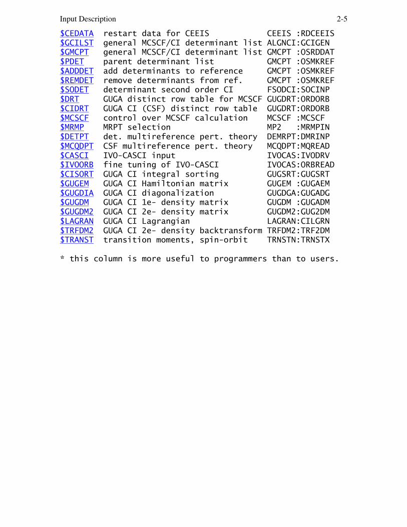
$CEDATA restart data for CEEIS CEEIS :RDCEEIS$GCILST general MCSCF/CI determinant list ALGNCI:GCIGEN$GMCPT general MCSCF/CI determinant list GMCPT :OSRDDAT$PDET parent determinant list GMCPT :OSMKREF$ADDDET add determinants to reference GMCPT :OSMKREF$REMDET remove determinants from ref. GMCPT :OSMKREF$SODET determinant second order CI FSODCI:SOCINP$DRT GUGA distinct row table for MCSCF GUGDRT:ORDORB$CIDRT GUGA CI (CSF) distinct row table GUGDRT:ORDORB$MCSCF control over MCSCF calculation MCSCF :MCSCF$MRMP MRPT selection MP2 :MRMPIN$DETPT det. multireference pert. theory DEMRPT:DMRINP$MCQDPT CSF multireference pert. theory MCQDPT:MQREAD$CASCI IVO-CASCI input IVOCAS:IVODRV$IVOORB fine tuning of IVO-CASCI IVOCAS:ORBREAD$CISORT GUGA CI integral sorting GUGSRT:GUGSRT$GUGEM GUGA CI Hamiltonian matrix GUGEM :GUGAEM$GUGDIA GUGA CI diagonalization GUGDGA:GUGADG$GUGDM GUGA CI 1e- density matrix GUGDM :GUGADM$GUGDM2 GUGA CI 2e- density matrix GUGDM2:GUG2DM$LAGRAN GUGA CI Lagrangian LAGRAN:CILGRN$TRFDM2 GUGA CI 2e- density backtransform TRFDM2:TRF2DM$TRANST transition moments, spin-orbit TRNSTN:TRNSTX
* this column is more useful to programmers than to users.
Input Description $CONTRL 2-6
==========================================================
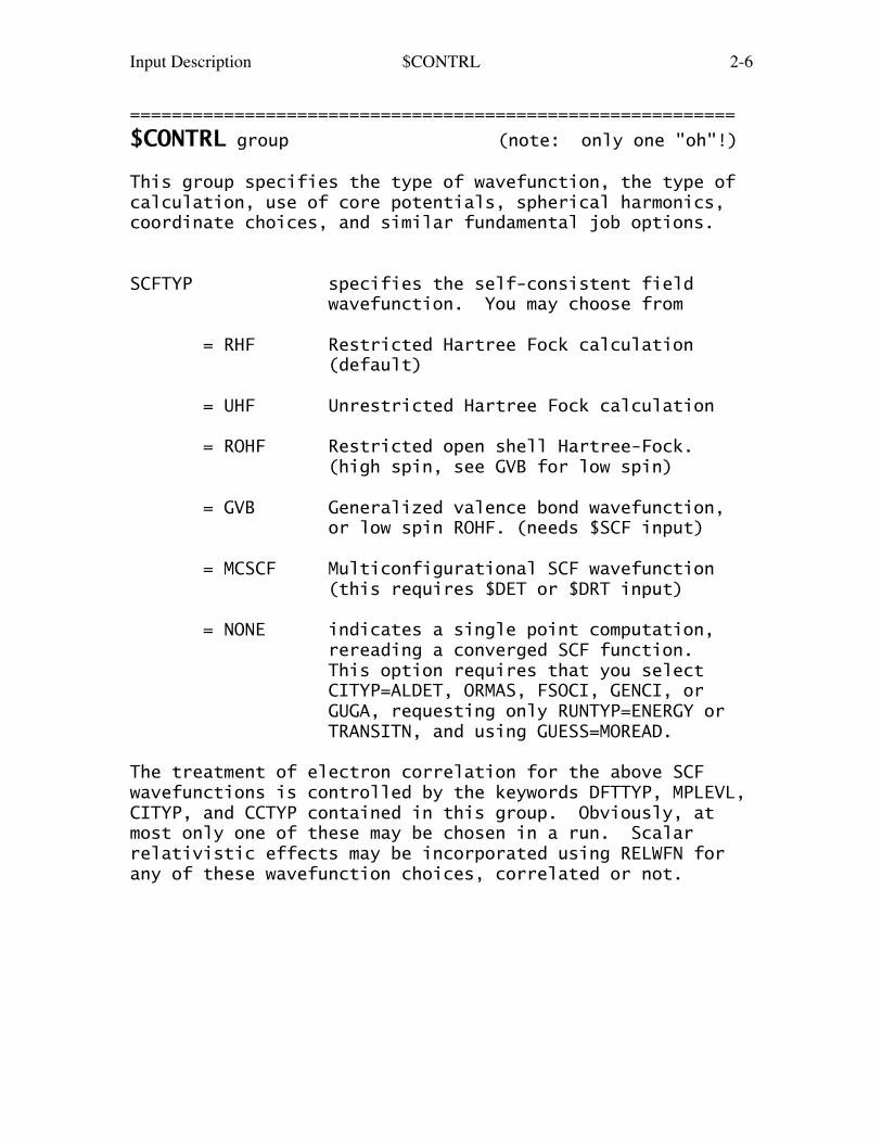
$CONTRL group (note: only one "oh"!)
This group specifies the type of wavefunction, the type ofcalculation, use of core potentials, spherical harmonics,coordinate choices, and similar fundamental job options.
SCFTYP specifies the self-consistent field wavefunction. You may choose from
= RHF Restricted Hartree Fock calculation (default)
= UHF Unrestricted Hartree Fock calculation
= ROHF Restricted open shell Hartree-Fock. (high spin, see GVB for low spin)
= GVB Generalized valence bond wavefunction, or low spin ROHF. (needs $SCF input)
= MCSCF Multiconfigurational SCF wavefunction (this requires $DET or $DRT input)
= NONE indicates a single point computation, rereading a converged SCF function. This option requires that you select CITYP=ALDET, ORMAS, FSOCI, GENCI, or GUGA, requesting only RUNTYP=ENERGY or TRANSITN, and using GUESS=MOREAD.
The treatment of electron correlation for the above SCFwavefunctions is controlled by the keywords DFTTYP, MPLEVL,CITYP, and CCTYP contained in this group. Obviously, atmost only one of these may be chosen in a run. Scalarrelativistic effects may be incorporated using RELWFN forany of these wavefunction choices, correlated or not.
Input Description $CONTRL 2-7
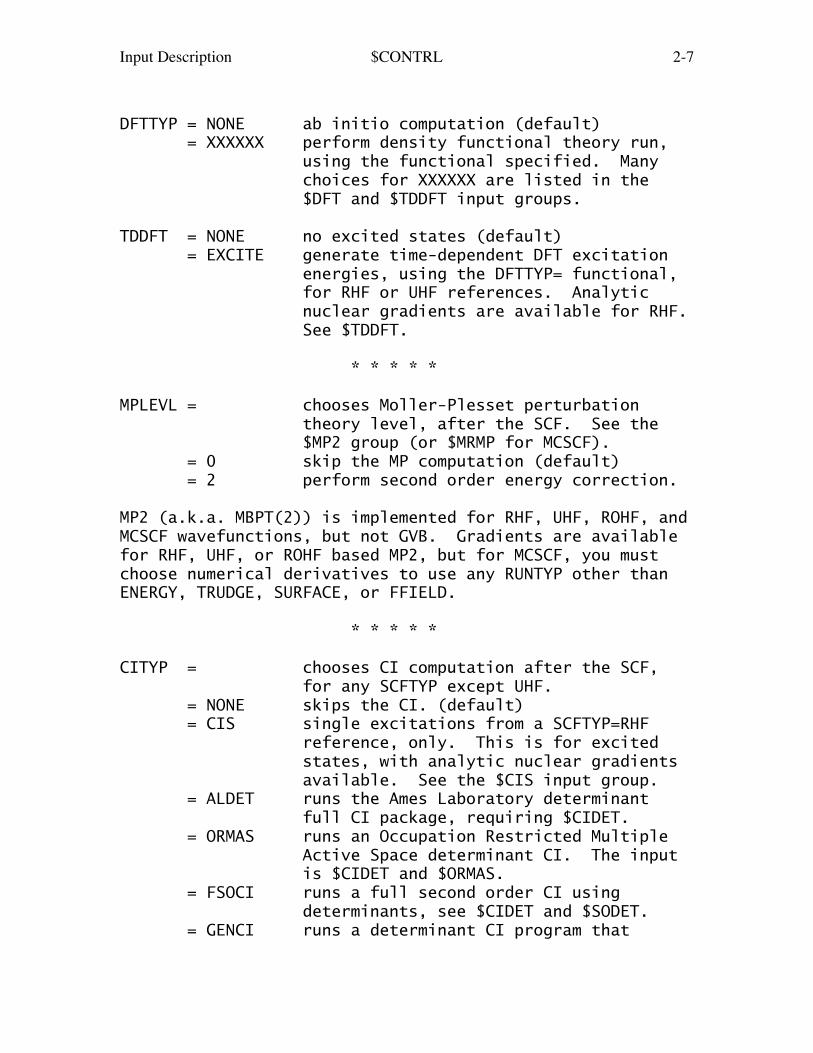
DFTTYP = NONE ab initio computation (default) = XXXXXX perform density functional theory run, using the functional specified. Many choices for XXXXXX are listed in the $DFT and $TDDFT input groups.
TDDFT = NONE no excited states (default) = EXCITE generate time-dependent DFT excitation energies, using the DFTTYP= functional, for RHF or UHF references. Analytic nuclear gradients are available for RHF. See $TDDFT.
* * * * *
MPLEVL = chooses Moller-Plesset perturbation theory level, after the SCF. See the $MP2 group (or $MRMP for MCSCF). = 0 skip the MP computation (default) = 2 perform second order energy correction.
MP2 (a.k.a. MBPT(2)) is implemented for RHF, UHF, ROHF, andMCSCF wavefunctions, but not GVB. Gradients are availablefor RHF, UHF, or ROHF based MP2, but for MCSCF, you mustchoose numerical derivatives to use any RUNTYP other thanENERGY, TRUDGE, SURFACE, or FFIELD.
* * * * *
CITYP = chooses CI computation after the SCF, for any SCFTYP except UHF. = NONE skips the CI. (default) = CIS single excitations from a SCFTYP=RHF reference, only. This is for excited states, with analytic nuclear gradients available. See the $CIS input group. = ALDET runs the Ames Laboratory determinant full CI package, requiring $CIDET. = ORMAS runs an Occupation Restricted Multiple Active Space determinant CI. The input is $CIDET and $ORMAS. = FSOCI runs a full second order CI using determinants, see $CIDET and $SODET. = GENCI runs a determinant CI program that
Input Description $CONTRL 2-8
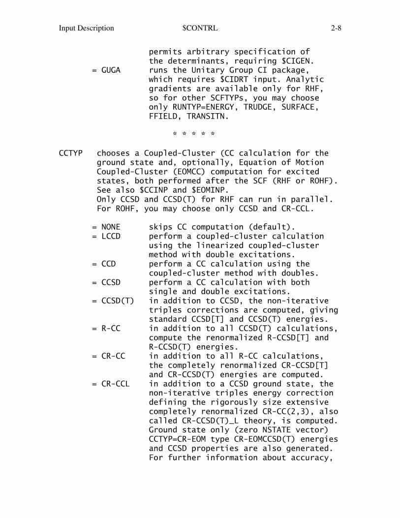
permits arbitrary specification of the determinants, requiring $CIGEN. = GUGA runs the Unitary Group CI package, which requires $CIDRT input. Analytic gradients are available only for RHF, so for other SCFTYPs, you may choose only RUNTYP=ENERGY, TRUDGE, SURFACE, FFIELD, TRANSITN.
* * * * *
CCTYP chooses a Coupled-Cluster (CC calculation for the ground state and, optionally, Equation of Motion Coupled-Cluster (EOMCC) computation for excited states, both performed after the SCF (RHF or ROHF). See also $CCINP and $EOMINP. Only CCSD and CCSD(T) for RHF can run in parallel. For ROHF, you may choose only CCSD and CR-CCL.
= NONE skips CC computation (default). = LCCD perform a coupled-cluster calculation using the linearized coupled-cluster method with double excitations. = CCD perform a CC calculation using the coupled-cluster method with doubles. = CCSD perform a CC calculation with both single and double excitations. = CCSD(T) in addition to CCSD, the non-iterative triples corrections are computed, giving standard CCSD[T] and CCSD(T) energies. = R-CC in addition to all CCSD(T) calculations, compute the renormalized R-CCSD[T] and R-CCSD(T) energies. = CR-CC in addition to all R-CC calculations, the completely renormalized CR-CCSD[T] and CR-CCSD(T) energies are computed. = CR-CCL in addition to a CCSD ground state, the non-iterative triples energy correction defining the rigorously size extensive completely renormalized CR-CC(2,3), also called CR-CCSD(T)_L theory, is computed. Ground state only (zero NSTATE vector) CCTYP=CR-EOM type CR-EOMCCSD(T) energies and CCSD properties are also generated. For further information about accuracy,
Input Description $CONTRL 2-9
and A to D CR-CC(2,3) energy types, see REFS.DOC. = CCSD(TQ) in addition to all R-CC calculations, non-iterative triple and quadruple corrections are used, to give CCSD(TQ) and various R-CCSD(TQ) energies. = CR-CC(Q) in addition to all CR-CC and CCSD(TQ) calculations, the CR-CCSD(TQ) energies are obtained.
= EOM-CCSD in addition to a CCSD ground state, excited states are calculated using the equation of motion coupled-cluster method with singles and doubles. = CR-EOM in addition to the CCSD and EOM-CCSD, noniterative triples corrections to CCSD ground-state and EOM-CCSD excited-state energies are found, using completely renormalized CR-EOMCCSD(T) approaches.
Any publication describing the results of CC calculationsobtained using GAMESS should reference the appropriatepapers, which are listed on the output of every run, and inchapter 4 of this manual.
Analytic gradients are not available, so use CCTYP only forRUNTYP=ENERGY, TRUDGE, SURFACE, or maybe FFIELD, or requestnumerical derivatives.
Generally speaking, the Renormalized energies are obtainedat similar cost to the standard values, while CompletelyRenormalized energies cost twice the time. For usage tipsand more information about resources on the various CoupledCluster methods, see Section 4, 'Further Information'.
* * * * *
RELWFN = NONE (default) See also the $RELWFN input group. = DK Douglas-Kroll transformation, available at the 1st, 2nd, or 3rd order. = RESC relativistic elimination of small component, the method of T. Nakajima and K. Hirao, available at 2nd order only. = NESC normalised elimination of small component, the method of K. Dyall, 2nd order only.
Input Description $CONTRL 2-10
* * * * *
RUNTYP specifies the type of computation, for example at a single geometry point:
= ENERGY Molecular energy. (default) = GRADIENT Molecular energy plus gradient. = HESSIAN Molecular energy plus gradient plus second derivatives, including harmonic harmonic vibrational analysis. See the $FORCE and $CPHF input groups. = GAMMA Evaluate up to 3rd nuclear derivatives, by finite differencing of Hessians. See $GAMMA, and also NFFLVL in $CONTRL.
multiple geometry options:
= OPTIMIZE Optimize the molecular geometry using analytic energy gradients. See $STATPT. = TRUDGE Non-gradient total energy minimization. See $TRUDGE and $TRURST. = SADPOINT Locate saddle point (transition state). See $STATPT. = MEX Locate minimum energy crossing point on the intersection seam of two potential energy surfaces. See $MEX. = IRC Follow intrinsic reaction coordinate. See $IRC. = VSCF anharmonic vibrational corrections. See $VSCF. = DRC Follow dynamic reaction coordinate. See $DRC. = MD molecular dynamics trajectory, see $MD. = GLOBOP Monte Carlo-type global optimization. See $GLOBOP. = OPTFMO genuine FMO geometry optimization using nearly analytic gradient. See $OPTFMO. = GRADEXTR Trace gradient extremal. See $GRADEX. = SURFACE Scan linear cross sections of the potential energy surface. See $SURF.
single geometry property options:
= G3MP2 evaluate heat of formation using the
Input Description $CONTRL 2-11
G3(MP2,CCSD(T)) methodology. See test example exam43.inp for more information. = PROP Properties will be calculated. A $DATA deck and converged $VEC deck should be input. Optionally, orbital localization can be done. See $ELPOT, etc. = RAMAN computes Raman intensities, see $RAMAN. = NACME non-adiabatic coupling matrix element between two or more state averaged MCSCF wavefunctions, of FORS/CAS type. The calculation has no special input group, but must use determinants. = NMR NMR shielding tensors for closed shell molecules by the GIAO method. See $NMR. = EDA Perform energy decomposition analysis. Give one of $MOROKM or $LMOEDA inputs. = TRANSITN Compute radiative transition moment or spin-orbit coupling. See $TRANST. = FFIELD applies finite electric fields, most commonly to extract polarizabilities. See $FFCALC. = TDHF analytic computation of time dependent polarizabilities. See $TDHF. = TDHFX extended TDHF package, including nuclear polarizability derivatives, and Raman and Hyper-Raman spectra. See $TDHFX. = MAKEFP creates an effective fragment potential, for SCFTYP=RHF or ROHF only. See $MAKEFP, $DAMP, $DAMPGS, $STONE, ... = FMO0 performs the free state FMO calculation. See $FMO.
* * * * * * * * * * * * * * * * * * * * * * * * * * * * * Note that RUNTYPs which require the nuclear gradient are GRADIENT, HESSIAN, OPTIMIZE, SADPOINT, GLOBOP, IRC, GRADEXTR, DRC, and RAMAN These are efficient with analytic gradients, which are available only for certain CI or MP2 calculations, but no CC calculations, as indicated above. See NUMGRD.* * * * * * * * * * * * * * * * * * * * * * * * * * * * *
NUMGRD Flag to allow numerical differentiation of the energy. Each gradient requires the energy be computed twice (forward and backward displacements) along each
Input Description $CONTRL 2-12
totally symmetric modes. It is thus recommended only for systems with just a few symmetry unique atoms in $DATA. The default is .FALSE.
EXETYP = RUN Actually do the run. (default) = CHECK Wavefunction and energy will not be evaluated. This lets you speedily check input and memory requirements. See the overview section for details. Note that you must set PARALL=.TRUE. in $SYSTEM to test distributed memory allocations. = DEBUG Massive amounts of output are printed, useful only if you hate trees. = routine Maximum output is generated by the routine named. Check the source for the routines this applies to.
* * * * * * *
ICHARG = Molecular charge. (default=0, neutral)
MULT = Multiplicity of the electronic state = 1 singlet (default) = 2,3,... doublet, triplet, and so on.
ICHARG and MULT are used directly for RHF, UHF, ROHF. For GVB, these are implicit in the $SCF input, while for MCSCF or CI, these are implicit in $DRT/$CIDRT or $DET/$CIDET input. You must still give them correctly.
* * * the next three control molecular geometry * * *
COORD = choice for molecular geometry in $DATA. = UNIQUE only the symmetry unique atoms will be given, in Cartesian coords (default). = HINT only the symmetry unique atoms will be given, in Hilderbrandt style internals. = PRINAXIS Cartesian coordinates will be input, and transformed to principal axes. Please read the warning just below!!! = ZMT GAUSSIAN style internals will be input. = ZMTMPC MOPAC style internals will be input. = FRAGONLY means no part of the system is treated
Input Description $CONTRL 2-13
by ab initio means, hence $DATA is not given. The system is defined by $EFRAG.
Note: the choices PRINAXIS, ZMT, ZMTMPC require input ofall atoms in the molecule. They also orient the molecule,and then determine which atoms are unique. Thereorientation is likely to change the order of the atomsfrom what you input. When the point group contains a 3-fold or higher rotation axis, the degenerate moments ofinertia often cause problems choosing correct symmetryunique axes, in which case you must use COORD=UNIQUE ratherthan Z-matrices.
Warning: The reorientation into principal axes is doneonly for atomic coordinates, and is not applied to the axisdependent data in the following groups: $VEC, $HESS, $GRAD,$DIPDR, $VIB, nor Cartesian coords of effective fragmentsin $EFRAG. COORD=UNIQUE avoids reorientation, and thus isthe safest way to read these.
Note: the choices PRINAXIS, ZMT, ZMTMPC require the useof a group named $BASIS to define the basis set. The firsttwo choices might or might not use $BASIS, as you wish.
UNITS = distance units, any angles must be in degrees. = ANGS Angstroms (default) = BOHR Bohr atomic units
NZVAR = 0 Use Cartesian coordinates (default). = M If COORD=ZMT or ZMTMPC, and $ZMAT is not given: the internal coordinates will be those defining the molecule in $DATA. In this case, $DATA may not contain any dummy atoms. M is usually 3N-6, or 3N-5 for linear. = M For other COORD choices, or if $ZMAT is given: the internal coordinates will be those defined in $ZMAT. This allows more sophisticated internal coordinate choices. M is ordinarily 3N-6 (3N-5), unless $ZMAT has linear bends.
NZVAR refers mainly to the coordinates used by OPTIMIZE or SADPOINT runs, but may also print the internal's values for other run types. You can use internals to define the molecule, but Cartesians during optimizations!
Input Description $CONTRL 2-14
* * * * * * *
Pseudopotentials may be of two types: ECP (effective corepotentials) which generate nodeless valence orbitals, andMCP (model core potentials) producing valence orbitals withthe correct radial nodal structure. At present, ECPs haveanalytic nuclear gradients and Hessians, while MCPs haveanalytic nuclear gradients.
PP = pseudopotential selection. = NONE all electron calculation (default). = READ read ECP potentials in the $ECP group. = SBKJC use Stevens, Basch, Krauss, Jasien, Cundari ECP potentials for all heavy atoms (Li-Rn are available). = HW use Hay, Wadt ECP potentials for heavy atoms (Na-Xe are available). = MCP use Huzinaga's Model Core Potentials. The correct MCP potential will be chosen to match the requested MCP valence basis set (see $BASIS).
* * * * * * *
LOCAL = controls orbital localization. = NONE Skip localization (default). = BOYS Do Foster-Boys localization. = RUEDNBRG Do Edmiston-Ruedenberg localization. = POP Do Pipek-Mezey population localization. See the $LOCAL group. Localization does not work for SCFTYP=GVB or CITYP.
* * * * * * *
ISPHER = Spherical Harmonics option = -1 Use Cartesian basis functions to construct symmetry-adapted linear combination (SALC) of basis functions. The SALC space is the linear variation space used. (default) = 0 Use spherical harmonic functions to create SALC functions, which are then expressed in terms of Cartesian functions. The contaminants are not dropped, hence this option has EXACTLY the same variational space as ISPHER=-1. The only benefit to
Input Description $CONTRL 2-15
obtain from this is a population analysis in terms of pure s,p,d,f,g functions. = +1 Same as ISPHER=0, but the function space is truncated to eliminate all contaminant Cartesian functions [3S(D), 3P(F), 4S(G), and 3D(G)] before constructing the SALC functions. The computation corresponds to the use of a spherical harmonic basis.
QMTTOL = linear dependence threshhold Any functions in the SALC variational space whose eigenvalue of the overlap matrix is below this tolerence is considered to be linearly dependent. Such functions are dropped from the variational space. What is dropped is not individual basis functions, but rather some linear combination(s) of the entire basis set that represent the linear dependent part of the function space. The default is a reasonable value for most purposes, 1.0E-6.
When many diffuse functions are used, it is common to see the program drop some combinations. On occasion, in multi-ring molecules, we have raised QMTTOL to 3.0E-6 to obtain SCF convergence, at the cost of some energy.
MAXIT = Maximum number of SCF iteration cycles. This pertains only to RHF, UHF, ROHF, or GVB runs. See also MAXIT in $MCSCF. (default = 30)
* * * interfaces to other programs * * *
MOLPLT = flag that produces an input deck for a molecule drawing program distributed with GAMESS. (default is .FALSE.)
PLTORB = flag that produces an input deck for an orbital plotting program distributed with GAMESS. (default is .FALSE.)
AIMPAC = flag to create an input deck for Bader's Atoms In Molecules properties code. (default=.FALSE.) For information about this program, see the URL http://www.chemistry.mcmaster.ca/faculty/bader/aim
Input Description $CONTRL 2-16
FRIEND = string to prepare input to other quantum programs, choose from = HONDO for HONDO 8.2 = MELDF for MELDF = GAMESSUK for GAMESS (UK Daresbury version) = GAUSSIAN for Gaussian 9x = ALL for all of the above
PLTORB, MOLPLT, and AIMPAC decks are written to filePUNCH at the end of the job. Thus all of these correspondto the final geometry encountered during jobs such asOPTIMIZE, SAPDOINT, IRC...
In contrast, selecting FRIEND turns the job into aCHECK run only, no matter how you set EXETYP. Thus thegeometry is that encountered in $DATA. The input isadded to the PUNCH file, and may require some (usuallyminimal) massaging.
PLTORB and MOLPLT are written even for EXETYP=CHECK.AIMPAC requires at least RUNTYP=PROP.
* * *
NFFLVL used to determine energies and gradients away from equilibrium structures, at the coordinates given in $DATA. The method will use a Taylor expansion of the potential surface around the stationary point. See $EQGEOM, $HLOWT, $GLOWT. This may be used with RUNTYP=ENERGY or GRADIENT. = 2 uses only Hessian information, which gives a reasonable energy, but not such a good gradient. = 3 uses Hessian and 3rd nuclear derivatives in the Taylor expansion, producing more accurate values for the energy and for the gradient.
* * * computation control switches * * *
For the most part, the default is the only sensiblevalue, and unless you are sure of what you are doing,these probably should not be touched.
NPRINT = Print/punch control flag
Input Description $CONTRL 2-17
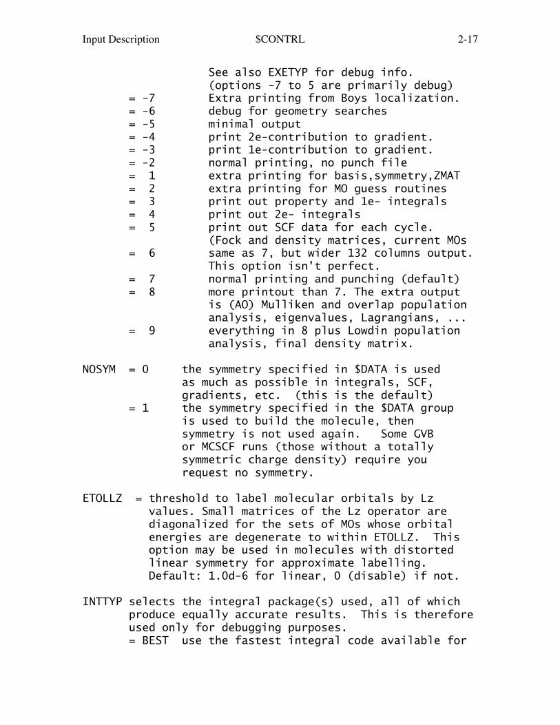
See also EXETYP for debug info. (options -7 to 5 are primarily debug) = -7 Extra printing from Boys localization. = -6 debug for geometry searches = -5 minimal output = -4 print 2e-contribution to gradient. = -3 print 1e-contribution to gradient. = -2 normal printing, no punch file = 1 extra printing for basis,symmetry,ZMAT = 2 extra printing for MO guess routines = 3 print out property and 1e- integrals = 4 print out 2e- integrals = 5 print out SCF data for each cycle. (Fock and density matrices, current MOs = 6 same as 7, but wider 132 columns output. This option isn't perfect. = 7 normal printing and punching (default) = 8 more printout than 7. The extra output is (AO) Mulliken and overlap population analysis, eigenvalues, Lagrangians, ... = 9 everything in 8 plus Lowdin population analysis, final density matrix.
NOSYM = 0 the symmetry specified in $DATA is used as much as possible in integrals, SCF, gradients, etc. (this is the default) = 1 the symmetry specified in the $DATA group is used to build the molecule, then symmetry is not used again. Some GVB or MCSCF runs (those without a totally symmetric charge density) require you request no symmetry.
ETOLLZ = threshold to label molecular orbitals by Lz values. Small matrices of the Lz operator are diagonalized for the sets of MOs whose orbital energies are degenerate to within ETOLLZ. This option may be used in molecules with distorted linear symmetry for approximate labelling. Default: 1.0d-6 for linear, 0 (disable) if not.
INTTYP selects the integral package(s) used, all of which produce equally accurate results. This is therefore used only for debugging purposes. = BEST use the fastest integral code available for

Input Description $CONTRL 2-18
any particular shell quartet (default): s,p,L or s,p,d,L rotated axis code first. ERIC s,p,d,f,g precursor transfer equation code second, up to 5 units total ang. mom. Rys quadrature for general s,p,d,f,g,L, or for uncontracted quartets. = ROTAXIS means don't use ERIC at all, e.g. rotated axis codes, or else Rys quadrature. = ERIC means don't use rotated axis codes, e.g. ERIC code, or else Rys quadrature. = RYSQUAD means use Rys quadrature for everything.
GRDTYP = BEST use the Schlegel routines for sp gradient blocks, and HONDO/Rys polynomial code for all other gradient integrals. (default) = HONDO use HONDO/Rys for all integral derivatives. This option produces very slightly more accurate gradients but is rather slower.
NORMF = 0 normalize the basis functions (default) = 1 no normalization
NORMP = 0 input contraction coefficients refer to normalized Gaussian primitives. (default) = 1 the opposite.
ITOL = primitive cutoff factor (default=20) = n products of primitives whose exponential factor is less than 10**(-n) are skipped.
ICUT = n integrals less than 10.0**(-n) are not saved on disk. (default = 9). Direct SCF will calculate to a cutoff 1.0d-10 or 5.0d-11 depending on FDIFF=.F. or .T.
ISKPRP = 0 proceed as usual 1 skip computation of some properties which are not well parallelised. This includes bond orders and virial theorem, and can help parallel scalability if many CPUs are used. Note that NPRINT=-5 disables most property computations as well, so ISKPRP=1 has no effect in that case. (default: 0)
Input Description $CONTRL 2-19
* * * restart options * * *
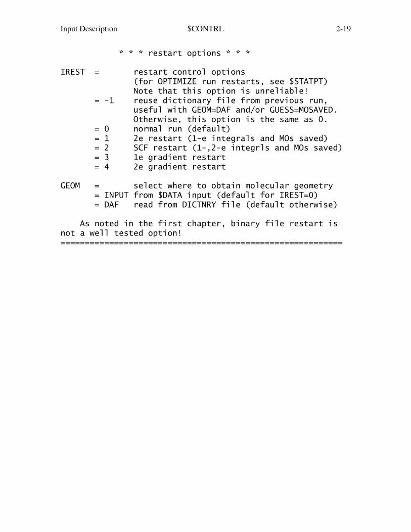
IREST = restart control options (for OPTIMIZE run restarts, see $STATPT) Note that this option is unreliable! = -1 reuse dictionary file from previous run, useful with GEOM=DAF and/or GUESS=MOSAVED. Otherwise, this option is the same as 0. = 0 normal run (default) = 1 2e restart (1-e integrals and MOs saved) = 2 SCF restart (1-,2-e integrls and MOs saved) = 3 1e gradient restart = 4 2e gradient restart
GEOM = select where to obtain molecular geometry = INPUT from $DATA input (default for IREST=0) = DAF read from DICTNRY file (default otherwise)
As noted in the first chapter, binary file restart isnot a well tested option!==========================================================
Input Description $SYSTEM 2-20
==========================================================
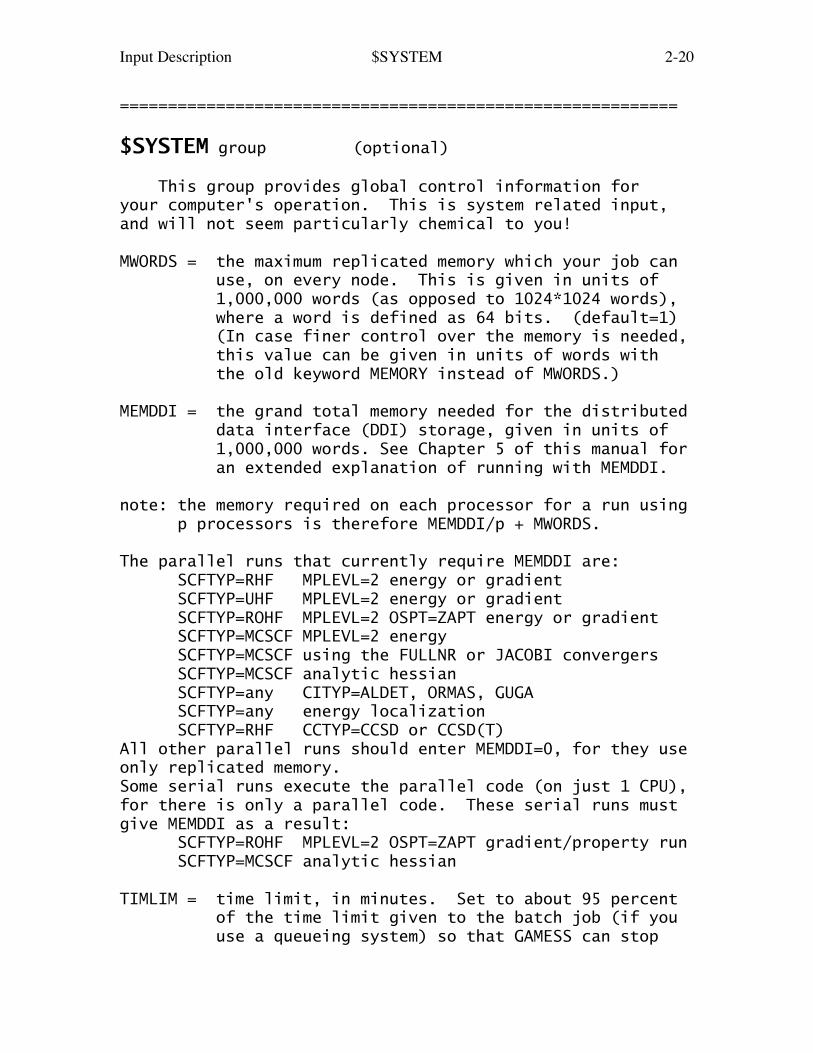
$SYSTEM group (optional)
This group provides global control information foryour computer's operation. This is system related input,and will not seem particularly chemical to you!
MWORDS = the maximum replicated memory which your job can use, on every node. This is given in units of 1,000,000 words (as opposed to 1024*1024 words), where a word is defined as 64 bits. (default=1) (In case finer control over the memory is needed, this value can be given in units of words with the old keyword MEMORY instead of MWORDS.)
MEMDDI = the grand total memory needed for the distributed data interface (DDI) storage, given in units of 1,000,000 words. See Chapter 5 of this manual for an extended explanation of running with MEMDDI.
note: the memory required on each processor for a run using p processors is therefore MEMDDI/p + MWORDS.
The parallel runs that currently require MEMDDI are: SCFTYP=RHF MPLEVL=2 energy or gradient SCFTYP=UHF MPLEVL=2 energy or gradient SCFTYP=ROHF MPLEVL=2 OSPT=ZAPT energy or gradient SCFTYP=MCSCF MPLEVL=2 energy SCFTYP=MCSCF using the FULLNR or JACOBI convergers SCFTYP=MCSCF analytic hessian SCFTYP=any CITYP=ALDET, ORMAS, GUGA SCFTYP=any energy localization SCFTYP=RHF CCTYP=CCSD or CCSD(T)All other parallel runs should enter MEMDDI=0, for they useonly replicated memory.Some serial runs execute the parallel code (on just 1 CPU),for there is only a parallel code. These serial runs mustgive MEMDDI as a result: SCFTYP=ROHF MPLEVL=2 OSPT=ZAPT gradient/property run SCFTYP=MCSCF analytic hessian
TIMLIM = time limit, in minutes. Set to about 95 percent of the time limit given to the batch job (if you use a queueing system) so that GAMESS can stop

Input Description $SYSTEM 2-21
itself gently. (default=525600.0 minutes)
PARALL = a flag to cause the distributed data parallel MP2 program to execute the parallel algorithm, even if you are running on only one node. The main purpose of this is to allow you to do EXETYP=CHECK runs to learn what the correct value of MEMDDI needs to be.
KDIAG = diagonalization control switch = 0 use a vectorized diagonalization routine if one is available on your machine, else use EVVRSP. (default) = 1 use EVVRSP diagonalization. This may be more accurate than KDIAG=0. = 2 use GIVEIS diagonalization (not as fast or reliable as EVVRSP) = 3 use JACOBI diagonalization (this is the slowest method)
COREFL = a flag to indicate whether or not GAMESS should produce a "core" file for debugging when subroutine ABRT is called to kill a job. This variable pertains only to UNIX operating systems. (default=.FALSE.)
BALTYP = Parallel load balance scheme: = SLB uses static load balancing. = DLB uses dynamic load balancing (default). Dynamic load balancing attempts to spread out possibly unequal work assignments based on the rate at which different nodes complete tasks. For historical reasons, it is permissible to spell SLB as LOOP, and DLB as NXTVAL.
NODEXT = array specifying node extentions in GDDI for each file. Non-zero values force no extension. E.g., NODEXT(40)=1 forces file 40 (file numbers are unit numbers used in GAMESS, see "rungms" or PROG.DOC) to have the name of $JOB.F40 on all nodes, rather than $JOB.F40, $JOB.F40.001, $JOB.F40.002 etc. This is convenient for FMO restart jobs, so that the file name need not be changed for each node, when copying the restart file. Note that on machines when several CPUs use

Input Description $SYSTEM 2-22
the same directory (e.g., SMP) NODEXT should be zero. (default: all zeros)
IOSMP = Parallelise I/O on SMP machines with multiple hard disks. Two parameters are specified, whose meaning should be clear from the example. iosmp(1)=2,6 2 refers to the number of HDDs per SMP box. 6 is the location of the character in the file names that switches HDDs, i.e. if HDDs are mounted as /work1 and /work2, then 6 refers to the position of the number 1 in /work1. The file system should permit disks attached with directory names differing by one symbol. (default: 0,0, disable the feature)
==========================================================

Input Description $BASIS 2-23
==========================================================
$BASIS group (optional)
This group allows certain standard basis sets to beeasily requested. If this group is omitted, the basis setmust be given in the $DATA group input.
GBASIS requests various Gaussian basis sets.
* * * segemented contractions * * *
GBASIS = MINI - Huzinaga's 3 gaussian minimal basis set. Available H-Rn. = MIDI - Huzinaga's 21 split valence basis set. Available H-Rn. = STO - Pople's STO-NG minimal basis set. Available H-Xe, for NGAUSS=2,3,4,5,6. = N21 - Pople's N-21G split valence basis set. Available H-Xe, for NGAUSS=3. Available H-Ar, for NGAUSS=6. = N31 - Pople's N-31G split valence basis set. Available H-Ne,P-Cl for NGAUSS=4. Available H-He,C-F for NGAUSS=5. Available H-Kr, for NGAUSS=6, note that the bases for K,Ca,Ga-Kr were changed 9/2006. = N311 - Pople's "triple split" N-311G basis set. Available H-Ne, for NGAUSS=6. Selecting N311 implies MC for Na-Ar. = DZV - "double zeta valence" basis set. a synonym for DH for H,Li,Be-Ne,Al-Cl. (14s,9p,3d)/[5s,3p,1d] for K-Ca. (14s,11p,5d/[6s,4p,1d] for Ga-Kr. = DH - Dunning/Hay "double zeta" basis set. (3s)/[2s] for H. (9s,4p)/[3s,2p] for Li. (9s,5p)/[3s,2p] for Be-Ne. (11s,7p)/[6s,4p] for Al-Cl. = TZV - "triple zeta valence" basis set. (5s)/[3s] for H. (10s,3p)/[4s,3p] for Li. (10s,6p)/[5s,3p] for Be-Ne. a synonym for MC for Na-Ar. (14s,9p)/[8s,4p] for K-Ca.

Input Description $BASIS 2-24
(14s,11p,6d)/[10s,8p,3d] for Sc-Zn. = MC - McLean/Chandler "triple split" basis. (12s,9p)/[6s,5p] for Na-Ar. Selecting MC implies 6-311G for H-Ne.
NGAUSS = the number of Gaussians (N). This parameter pertains only to GBASIS=STO, N21, N31, or N311.
Note: Polarization functions and/or diffuse functions areto be added separately to these GBASIS values, which defineonly the atom's occupied orbitals, with keywords such asNDFUNC and DIFFSP. Pople GBASIS keywords require NGAUSS.
* * * systematic basis set families * * *
GBASIS = CCn - Dunning-type Correlation Consistent basis sets, officially called cc-pVnZ. Use n = D,T,Q,5,6 to indicate the level of polarization. These provide a hierachy of basis sets suitable for recovering the correlation energy. Available for H-He, Li-Ne, Na-Ar, Ca, Ga-Kr and for Sc-Zn for n=T,Q. = ACCn - As CCn, but augmented with a set of diffuse functions, e.g. aug-cc-pVnZ. = CCnC - As CCn, but augmented with tight functions for recovering core and core-valence correlation, e.g. cc-pCVnZ. = ACCnC- As CCn, but augmented with both tight and diffuse functions, e.g. aug-cc-pCVnZ. = PCn - Jensen Polarization Consistent basis sets. n = 0,1,2,3,4 indicates the level of polarization. (n=0 is unpolarized, n=1 is DZP, n=2 is TZ2P, etc.). These provide a hierachy of basis sets suitable for DFT and HF calculations. Available H-Ar. = APCn - As PCn, but augmented with a set of diffuse functions.
Notes:1. Normally these basis sets are used only as sphericalharmonics, see ISPHER=1 in $CONTRL.2. The CC5, CC6, and PC4 basis sets (and correspondingaugmented versions) contain h-functions, and CC6 containsi-functions. As GAMESS' integral codes are currently
Input Description $BASIS 2-25
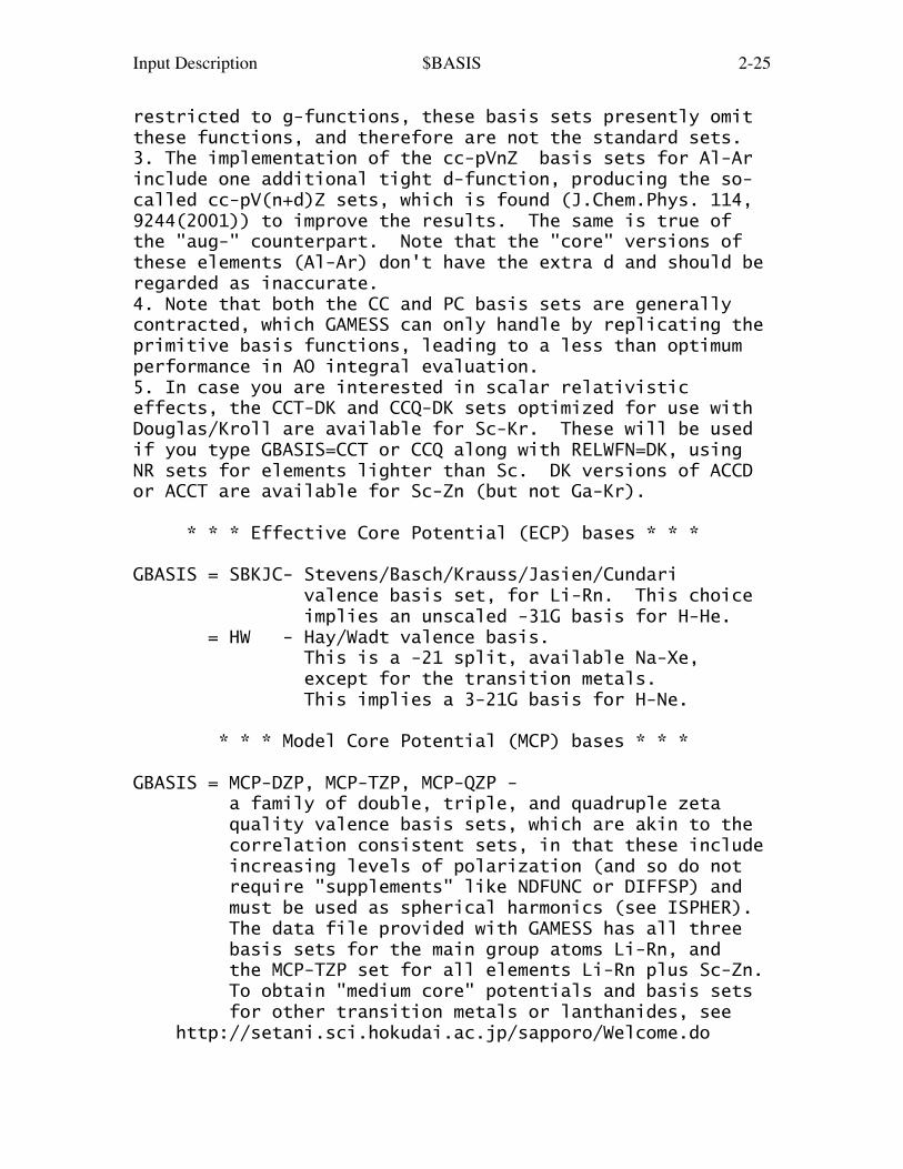
restricted to g-functions, these basis sets presently omitthese functions, and therefore are not the standard sets.3. The implementation of the cc-pVnZ basis sets for Al-Arinclude one additional tight d-function, producing the so-called cc-pV(n+d)Z sets, which is found (J.Chem.Phys. 114,9244(2001)) to improve the results. The same is true ofthe "aug-" counterpart. Note that the "core" versions ofthese elements (Al-Ar) don't have the extra d and should beregarded as inaccurate.4. Note that both the CC and PC basis sets are generallycontracted, which GAMESS can only handle by replicating theprimitive basis functions, leading to a less than optimumperformance in AO integral evaluation.5. In case you are interested in scalar relativisticeffects, the CCT-DK and CCQ-DK sets optimized for use withDouglas/Kroll are available for Sc-Kr. These will be usedif you type GBASIS=CCT or CCQ along with RELWFN=DK, usingNR sets for elements lighter than Sc. DK versions of ACCDor ACCT are available for Sc-Zn (but not Ga-Kr).
* * * Effective Core Potential (ECP) bases * * *
GBASIS = SBKJC- Stevens/Basch/Krauss/Jasien/Cundari valence basis set, for Li-Rn. This choice implies an unscaled -31G basis for H-He. = HW - Hay/Wadt valence basis. This is a -21 split, available Na-Xe, except for the transition metals. This implies a 3-21G basis for H-Ne.
* * * Model Core Potential (MCP) bases * * *
GBASIS = MCP-DZP, MCP-TZP, MCP-QZP - a family of double, triple, and quadruple zeta quality valence basis sets, which are akin to the correlation consistent sets, in that these include increasing levels of polarization (and so do not require "supplements" like NDFUNC or DIFFSP) and must be used as spherical harmonics (see ISPHER). The data file provided with GAMESS has all three basis sets for the main group atoms Li-Rn, and the MCP-TZP set for all elements Li-Rn plus Sc-Zn. To obtain "medium core" potentials and basis sets for other transition metals or lanthanides, see http://setani.sci.hokudai.ac.jp/sapporo/Welcome.do
Input Description $BASIS 2-26
= IMCP-SR1 and IMCP-SR2 - valence basis sets to be used with the improved MCPs with scalar relativistic effects. These are available for transition metals except La, and the main group elements B-Ne, P-Ar, Ge, Kr, Sb, Xe, Rn. The 1 and 2 refer to addition of first and second polarization shells, so again don't use any of the "supplements" and do use spherical harmonics. = IMCP-NR1 and IMCP-NR2 - closely related valence basis sets, but with nonrelativistic model core potentials.
Notes: Select PP=MCP in $CONTRL to automatically use themodel core potential matching your basis choice. Note thatreferences for these bases, and other information aboutMCPs can be found in the REFS.DOC chapter. Another familycovering almost all elements is available in $DATA only.
* * * semiempirical basis sets * * *
GBASIS = MNDO - selects MNDO model hamiltonian = AM1 - selects AM1 model hamiltonian = PM3 - selects PM3 model hamiltonian
Note: The elements for which these exist can be found inthe 'further information' section of this manual. If youpick one of these, all other data in this group is ignored.Semi-empirical runs actually use valence-only Slater typeorbitals (STOs), not Gaussian GTOs, but the keyword remainsGBASIS. NDFUNC, etc. will be ignored for these.
--- supplementary functions ---
NDFUNC = number of heavy atom polarization functions to be used. These are usually d functions, except for MINI/MIDI. The term "heavy" means Na on up when GBASIS=STO, HW, or N21, and from Li on up otherwise. The value may not exceed 3. The variable POLAR selects the actual exponents to be used, see also SPLIT2 and SPLIT3. (default=0)
NFFUNC = number of heavy atom f type polarization functions to be used on Li-Cl. This may only be input as 0 or 1. (default=0)
Input Description $BASIS 2-27
NPFUNC = number of light atom, p type polarization functions to be used on H-He. This may not exceed 3, see also POLAR. (default=0)
DIFFSP = flag to add diffuse sp (L) shell to heavy atoms. Heavy means Li-F, Na-Cl, Ga-Br, In-I, Tl-At. The default is .FALSE.
DIFFS = flag to add diffuse s shell to hydrogens. The default is .FALSE.
Warning: if you use diffuse functions, please read QMTTOLin the $CONTRL group for numerical concerns.
POLAR = exponent of polarization functions = COMMON (default for GBASIS=STO,N21,HW,SBKJC) = POPN31 (default for GBASIS=N31) = POPN311 (default for GBASIS=N311, MC) = DUNNING (default for GBASIS=DH, DZV) = HUZINAGA (default for GBASIS=MINI, MIDI) = HONDO7 (default for GBASIS=TZV)
SPLIT2 = an array of splitting factors used when NDFUNC or NPFUNC is 2. Default=2.0,0.5
SPLIT3 = an array of splitting factors used when NDFUNC or NPFUNC is 3. Default=4.00,1.00,0.25
EXTFIL = a flag to read basis sets from an external file, defined by EXTBAS, rather than from a $DATA group. (default=.false.)
Except for MCP basis sets, no external file is providedwith GAMESS, thus you must create your own. The GBASISkeyword must give an 8 or less character string, obviouslynot using any internally stored names. Every atom must bedefined in the external file by a line giving the chemicalsymbol, and this chosen string. Following this header line,give the basis in free format $DATA style, containing onlyS, P, D, F, G, and L shells, and terminating each atom bythe usual blank line. The external file may have severalfamilies of bases in the same file, identified by differentGBASIS strings.=========================================================
Input Description $BASIS 2-28
The splitting factors are from the Pople school, and areprobably too far apart. See for example the Binning andCurtiss paper. For example, the SPLIT2 value will usuallycause an INCREASE over the 1d energy at the HF level forhydrocarbons.
The actual exponents used for polarization functions, aswell as for diffuse sp or s shells, are described in the'Further References' section of this manual. This sectionalso describes the sp part of the basis set chosen byGBASIS fully, with all references cited.
Note that GAMESS always punches a full $DATA group. Thus,if $BASIS does not quite cover the basis you want, you canobtain this full $DATA group from EXETYP=CHECK, and thenchange polarization exponents, add Rydbergs, etc.
Input Description $DATA 2-29
==========================================================
$DATA group (required)$DATAS group (if NESC chosen, for small component basis)$DATAL group (if NESC chosen, for large component basis)
This group describes the global molecular data such aspoint group symmetry, nuclear coordinates, and possiblythe basis set. It consists of a series of free formatcard images. See $RELWFN for more information on large andsmall component basis sets. The input structure of $DATASand $DATAL is identical to the COORD=UNIQUE $DATA input.
----------------------------------------------------------
-1- TITLE a single descriptive title card.
----------------------------------------------------------
-2- GROUP, NAXIS
GROUP is the Schoenflies symbol of the symmetry group,you may choose from C1, Cs, Ci, Cn, S2n, Cnh, Cnv, Dn, Dnh, Dnd, T, Th, Td, O, Oh.
NAXIS is the order of the highest rotation axis, andmust be given when the name of the group contains an N.For example, "Cnv 2" is C2v. "S2n 3" means S6. Use ofNAXIS up to 8 is supported in each axial groups.
For linear molecules, choose either Cnv or Dnh, and enterNAXIS as 4. Enter atoms as Dnh with NAXIS=2. If theelectronic state of either is degenerate, check the noteabout the effect of symmetry in the electronic statein the SCF section of REFS.DOC.
----------------------------------------------------------
In order to use GAMESS effectively, you must be ableto recognize the point group name for your molecule. Thispresupposes a knowledge of group theory at about the levelof Cotton's "Group Theory", Chapter 3.
Input Description $DATA 2-30
Armed with only the name of the group, GAMESS is ableto exploit the molecular symmetry throughout almost all ofthe program, and thus save a great deal of computer time.GAMESS does not require that you know very much else aboutgroup theory, although a deeper knowledge (charactertables, irreducible representations, term symbols, and soon) is useful when dealing with the more sophisticatedwavefunctions.
Cards -3- and -4- are quite complicated, and are rarelygiven. A *SINGLE* blank card may replace both cards -3-and -4-, to select the 'master frame', which is defined onthe next page. If you choose to enter a blank line, skipto one of the -5- input sequences.
Note!If the point group is C1 (no symmetry), skip over cards-3- and -4- (which means no blank card).
----------------------------------------------------------
-3- X1, Y1, Z1, X2, Y2, Z2
For C1 group, there is no card -3- or -4-.For CI group, give one point, the center of inversion.For CS group, any two points in the symmetry plane.For axial groups, any two points on the principal axis.For tetrahedral groups, any two points on a two-fold axis.For octahedral groups, any two points on a four-fold axis.
----------------------------------------------------------
-4- X3, Y3, Z3, DIRECT
third point, and a directional parameter.For CS group, one point of the symmetry plane, noncollinear with points 1 and 2.For CI group, there is no card -4-.
For other groups, a generator sigma-v plane (if any) isthe (x,z) plane of the local frame (CNV point groups).
A generator sigma-h plane (if any) is the (x,y) plane ofthe local frame (CNH and dihedral groups).

Input Description $DATA 2-31
A generator C2 axis (if any) is the x-axis of the localframe (dihedral groups).
The perpendicular to the principal axis passing throughthe third point defines a direction called D1. IfDIRECT='PARALLEL', the x-axis of the local frame coincideswith the direction D1. If DIRECT='NORMAL', the x-axis ofthe local frame is the common perpendicular to D1 and theprincipal axis, passing through the intersection point ofthese two lines. Thus D1 coincides in this case with thenegative y axis.
----------------------------------------------------------
The 'master frame' is just a standard orientation forthe molecule. By default, the 'master frame' assumes that 1. z is the principal rotation axis (if any), 2. x is a perpendicular two-fold axis (if any), 3. xz is the sigma-v plane (if any), and 4. xy is the sigma-h plane (if any).Use the lowest number rule that applies to your molecule.
Some examples of these rules:Ammonia (C3v): the unique H lies in the XZ plane (R1,R3).Ethane (D3d): the unique H lies in the YZ plane (R1,R2).Methane (Td): the H lies in the XYZ direction (R2). Since there is more than one 3-fold, R1 does not apply.HP=O (Cs): the mirror plane is the XY plane (R4).
In general, it is a poor idea to try to reorient themolecule. Certain sections of the program, such as theorbital symmetry assignment, do not know how to deal withcases where the 'master frame' has been changed.
Linear molecules (C4v or D4h) must lie along the z axis,so do not try to reorient linear molecules.
You can use EXETYP=CHECK to quickly find what atoms aregenerated, and in what order. This is typically necessaryin order to use the general $ZMAT coordinates.
* * * *
Depending on your choice for COORD in $CONTROL,
Input Description $DATA 2-32
if COORD=UNIQUE, follow card sequence U if COORD=HINT, follow card sequence U if COORD=CART, follow card sequence C if COORD=ZMT, follow card sequence G if COORD=ZMTMPC, follow card sequence M
Card sequence U is the only one which allows you to definea completely general basis here in $DATA.
Recall that UNIT in $CONTRL determines the distance units.
----------------------------------------------------------
-5U- Atom input. Only the symmetry unique atoms areinput, GAMESS will generate the symmetry equivalent atomsaccording to the point group selected above.
if COORD=UNIQUE NAME, ZNUC, X, Y, Z ***************
NAME = 10 character atomic name, used only for printout. Thus you can enter H or Hydrogen, or whatever.ZNUC = nuclear charge. It is the nuclear charge which actually defines the atom's identity.X,Y,Z = Cartesian coordinates.
if COORD=HINT *************
NAME,ZNUC,CONX,R,ALPHA,BETA,SIGN,POINT1,POINT2,POINT3
NAME = 10 character atomic name (used only for print out).ZNUC = nuclear charge.CONX = connection type, choose from 'LC' linear conn. 'CCPA' central conn. 'PCC' planar central conn. with polar atom 'NPCC' non-planar central conn. 'TCT' terminal conn. 'PTC' planar terminal conn. with torsionR = connection distance.ALPHA= first connection angleBETA = second connection angleSIGN = connection sign, '+' or '-'POINT1, POINT2, POINT3 = connection points, a serial number of a previously input atom, or one of 4 standard points: O,I,J,K
Input Description $DATA 2-33
(origin and unit points on axes of master frame). defaults: POINT1='O', POINT2='I', POINT3='J'
ref- R.L. Hilderbrandt, J.Chem.Phys. 51, 1654 (1969).You cannot understand HINT input without reading this.
Note that if ZNUC is negative, the internally storedbasis for ABS(ZNUC) is placed on this center, but thecalculation uses ZNUC=0 after this. This is usefulfor basis set superposition error (BSSE) calculations.----------------------------------------------------------
* * * If you gave $BASIS, continue entering cards -5U- until all the unique atoms have been specified. When you are done, enter a " $END " card.* * * If you did not, enter cards -6U-, -7U-, -8U-.
-----------------------------------------------------------6U- GBASIS, NGAUSS, (SCALF(i),i=1,4)
GBASIS has exactly the same meaning as in $BASIS. You maychoose from MINI, MIDI, STO, N21, N31, N311, DZV, DH, BC,TZV, MC, SBKJC, or HW. In addition, you may choose S, P,D, F, G, or L to enter an explicit basis set. Here, Lmeans both an s and p shell with a shared exponent.
In addition, GBASIS may be defined as MCP, to indicate thatthe current atom is represented by a model core potential,and valence basis set. An internally stored basis andpotential will be applied (see REFS.DOC for the details).The MCP basis supplies only the occupied atomic orbitals,e.g. sp for a main group element, so please supplement withany desired polarization. In case the keyword MCP isfollowed by the keyword READ, everything will be taken fromthe input file, namely the basis functions are read usingthe sequence -6U-, -7U-, and -8U-, from lines following the"MCP READ" line. In addition, "MCP READ" implies that theparameters of the model core potentials, together with corebasis functions are in the input stream, in a $MCP group.Other MCP bases are available in the $BASIS group, but notethat to locate the MCP, the atom name must be a chemicalsymbol, that is "P" instead of "Phosphorus".
Input Description $DATA 2-34
NGAUSS is the number of Gaussians (N) in the Pople stylebasis, or user input general basis. It has meaning onlyfor GBASIS=STO, N21, N31, or N311, and S,P,D,F,G, or L.
Up to 4 scale factors may be entered. If omitted, standardvalues are used. They are not documented as every GBASIStreats these differently. Read the source code if you needto know more. They are seldom given.----------------------------------------------------------
* * * If GBASIS is not S,P,D,F,G, or L, either add more shells by repeating card -6U-, or go on to -8U-.* * * If GBASIS=S,P,D,F,G, or L, enter NGAUSS cards -7U-.
-----------------------------------------------------------7U- IG, ZETA, C1, C2
IG = a counter, IG takes values 1, 2, ..., NGAUSS. ZETA = Gaussian exponent of the IG'th primitive. C1 = Contraction coefficient for S,P,D,F,G shells, and for the s function of L shells. C2 = Contraction coefficient for the p in L shells.----------------------------------------------------------
* * * For more shells on this atom, go back to card -6U-.* * * If there are no more shells, go on to card -8U-.
-----------------------------------------------------------8U- A blank card ends the basis set for this atom.----------------------------------------------------------
Continue entering atoms with -5U- through -8U- until allare given, then terminate the group with a " $END " card.
--- this is the end of card sequence U ---
COORD=CART input:
----------------------------------------------------------
-5C- Atom input.
Cartesian coordinates for all atoms must be entered. Theymay be arbitrarily rotated or translated, but must possessthe actual point group symmetry. GAMESS will reorient the

Input Description $DATA 2-35
molecule into the 'master frame', and determine whichatoms are the unique ones. Thus, the final order of theatoms may be different from what you enter here.
NAME, ZNUC, X, Y, Z
NAME = 10 character atomic name, used only for printout. Thus you can enter H or Hydrogen, or whatever.ZNUC = nuclear charge. It is the nuclear charge which actually defines the atom's identity.X,Y,Z = Cartesian coordinates.
----------------------------------------------------------
Continue entering atoms with card -5C- until all aregiven, and then terminate the group with a " $END " card.
--- this is the end of card sequence C ---
COORD=ZMT input: (GAUSSIAN style internals)
----------------------------------------------------------
-5G- ATOM
Only the name of the first atom is required.See -8G- for a description of this information.----------------------------------------------------------
-6G- ATOM i1 BLENGTH
Only a name and a bond distance is required for atom 2.See -8G- for a description of this information.----------------------------------------------------------
-7G- ATOM i1 BLENGTH i2 ALPHA
Only a name, distance, and angle are required for atom 3.See -8G- for a description of this information.----------------------------------------------------------
-8G- ATOM i1 BLENGTH i2 ALPHA i3 BETA i4
ATOM is the chemical symbol of this atom. It can be followed by numbers, if desired, for example Si3.
Input Description $DATA 2-36
The chemical symbol implies the nuclear charge.i1 defines the connectivity of the following bond.BLENGTH is the bond length "this atom-atom i1".i2 defines the connectivity of the following angle.ALPHA is the angle "this atom-atom i1-atom i2".i3 defines the connectivity of the following angle.BETA is either the dihedral angle "this atom-atom i1- atom i2-atom i3", or perhaps a second bond angle "this atom-atom i1-atom i3".i4 defines the nature of BETA, If BETA is a dihedral angle, i4=0 (default). If BETA is a second bond angle, i4=+/-1. (sign specifies one of two possible directions).----------------------------------------------------------
o Repeat -8G- for atoms 4, 5, ... o The use of ghost atoms is possible, by using X or BQ for the chemical symbol. Ghost atoms preclude the option of an automatic generation of $ZMAT. o The connectivity i1, i2, i3 may be given as integers, 1, 2, 3, 4, 5,... or as strings which match one of the ATOMs. In this case, numbers must be added to the ATOM strings to ensure uniqueness! o In -6G- to -8G-, symbolic strings may be given in place of numeric values for BLENGTH, ALPHA, and BETA. The same string may be repeated, which is handy in enforcing symmetry. If the string is preceeded by a minus sign, the numeric value which will be used is the opposite, of course. Any mixture of numeric data and symbols may be given. If any strings were given in -6G- to -8G-, you must provide cards -9G- and -10G-, otherwise you may terminate the group now with a " $END " card.
----------------------------------------------------------
-9G- A blank line terminates the Z-matrix section.
----------------------------------------------------------
-10G- STRING VALUE
STRING is a symbolic string used in the Z-matrix.VALUE is the numeric value to substitute for that string.
Input Description $DATA 2-37
----------------------------------------------------------
Continue entering -10G- until all STRINGs are defined.Note that any blank card encountered while reading -10G-will be ignored. GAMESS regards all STRINGs as variables(constraints are sometimes applied in $STATPT). It is notnecessary to place constraints to preserve point groupsymmetry, as GAMESS will never lower the symmetry fromthat given at -2-. When you have given all STRINGs aVALUE, terminate the group with a " $END " card.
--- this is the end of card sequence G ---
* * * *
The documentation for sequence G above and sequence Mbelow presumes you are reasonably familiar with the inputto GAUSSIAN or MOPAC. It is probably too terse to beunderstood very well if you are unfamiliar with these. Agood tutorial on both styles of Z-matrix input can befound in Tim Clark's book "A Handbook of ComputationalChemistry", published by John Wiley & Sons, 1985.
Both Z-matrix input styles must generate a moleculewhich possesses the symmetry you requested at -2-. Ifnot, your job will be terminated automatically.
COORD=ZMTMPC input: (MOPAC style internals)
----------------------------------------------------------
-5M- ATOM
Only the name of the first atom is required.See -8M- for a description of this information.----------------------------------------------------------
-6M- ATOM BLENGTH
Only a name and a bond distance is required for atom 2.See -8M- for a description of this information.----------------------------------------------------------
-7M- ATOM BLENGTH j1 ALPHA j2
Input Description $DATA 2-38
Only a bond distance from atom 2, and an angle with repectto atom 1 is required for atom 3. If you prefer to hookatom 3 to atom 1, you must give connectivity as in -8M-.See -8M- for a description of this information.----------------------------------------------------------
-8M- ATOM BLENGTH j1 ALPHA j2 BETA j3 i1 i2 i3
ATOM, BLENGTH, ALPHA, BETA, i1, i2 and i3 are as describedat -8G-. However, BLENGTH, ALPHA, and BETA must be givenas numerical values only. In addition, BETA is always adihedral angle. i1, i2, i3 must be integers only.
The j1, j2 and j3 integers, used in MOPAC to signaloptimization of parameters, must be supplied but areignored here. You may give them as 0, for example.----------------------------------------------------------
Continue entering atoms 3, 4, 5, ... with -8M- cards untilall are given, and then terminate the group by giving a" $END " card.
--- this is the end of card sequence M ---
========================================================== This is the end of $DATA!
If you have any doubt about what molecule and basis setyou are defining, or what order the atoms will begenerated in, simply execute an EXETYP=CHECK job to findout!
Input Description $ZMAT 2-39
==========================================================
$ZMAT group (required if NZVAR is nonzero in $CONTRL)
This group lets you define the internal coordinates inwhich the gradient geometry search is carried out. Theseneed not be the same as the internal coordinates used in$DATA. The coordinates may be simple Z-matrix types,delocalized coordinates, or natural internal coordinates.
You must input a total of M=3N-6 internal coordinates(M=3N-5 for linear molecules). NZVAR in $CONTRL can beless than M IF AND ONLY IF you are using linear bends. Itis also possible to input more than M coordinates if theyare used to form exactly M linear combinations for newinternals. These may be symmetry coordinates or naturalinternal coordinates. If NZVAR > M, you must input IJS andSIJ below to form M new coordinates. See DECOMP in $FORCEfor the only circumstance in which you may enter a largerNZVAR without giving SIJ and IJS.
**** IZMAT defines simple internal coordinates ****
IZMAT is an array of integers defining each coordinate.The general form for each internal coordinate is code number,I,J,K,L,M,N
IZMAT =1 followed by two atom numbers. (I-J bond length) =2 followed by three numbers. (I-J-K bond angle) =3 followed by four numbers. (dihedral angle) Torsion angle between planes I-J-K and J-K-L. =4 followed by four atom numbers. (atom-plane) Out-of-plane angle from bond I-J to plane J-K-L. =5 followed by three numbers. (I-J-K linear bend) Counts as 2 coordinates for the degenerate bend, normally J is the center atom. See $LIBE. =6 followed by five atom numbers. (dihedral angle) Dihedral angle between planes I-J-K and K-L-M. =7 followed by six atom numbers. (ghost torsion) Let A be the midpoint between atoms I and J, and B be the midpoint between atoms M and N. This coordinate is the dihedral angle A-K-L-B. The atoms I,J and/or M,N may be the same atom number. (If I=J AND M=N, this is a conventional torsion). Examples: N2H4, or, with one common pair, H2POH.

Input Description $ZMAT 2-40
Example - a nonlinear triatomic, atom 2 in the middle: $ZMAT IZMAT(1)=1,1,2, 2,1,2,3, 1,2,3 $ENDThis sets up two bonds and the angle between them.The blanks between each coordinate definition arenot necessary, but improve readability mightily.
**** the next define delocalized coordinates ****
DLC is a flag to request delocalized coordinates. (default is .FALSE.)
AUTO is a flag to generate all redundant coordinates, automatically. The DLC space will consist of all non-redundant combinations of these which can be found. The list of redundant coordinates will consist of bonds, angles, and torsions only. (default is .FALSE.)
NONVDW is an array of atom pairs which are to be joined by a bond, but might be skipped by the routine that automatically includes all distances shorter than the sum of van der Waals radii. Any angles and torsions associated with the new bond(s) are also automatically included.
The format for IXZMAT, IRZMAT, IFZMAT is that of IZMAT:
IXZMAT is an extra array of simple internal coordinates which you want to have added to the list generated by AUTO. Unlike NONVDW, IXZMAT will add only the coordinate(s) you specify.
IRZMAT is an array of simple internal coordinates which you would like to remove from the AUTO list of redundant coordinates. It is sometimes necessary to remove a torsion if other torsions around a bond are being frozen, to obtain a nonsingular G matrix.
IFZMAT is an array of simple internal coordinates which you would like to freeze. See also FVALUE below. IFZMAT/FVALUE work with ordinary coordinate input using IZMAT, as well as with DLC, but in the former case be careful that IFZMAT specifies coordinates
Input Description $ZMAT 2-41
that were already given in IZMAT. In addition, IFZMAT works only for IZMAT=1,2,3 type coordinates. See IFREEZ in $STATPT you wish to freeze regular or natural internal coordinates.
FVALUE is an array of values to which the internal coordinates should be constrained. It is not necessary to input $DATA such that the initial values match these desired final values, but it is helpful if the initial values are not too far away.
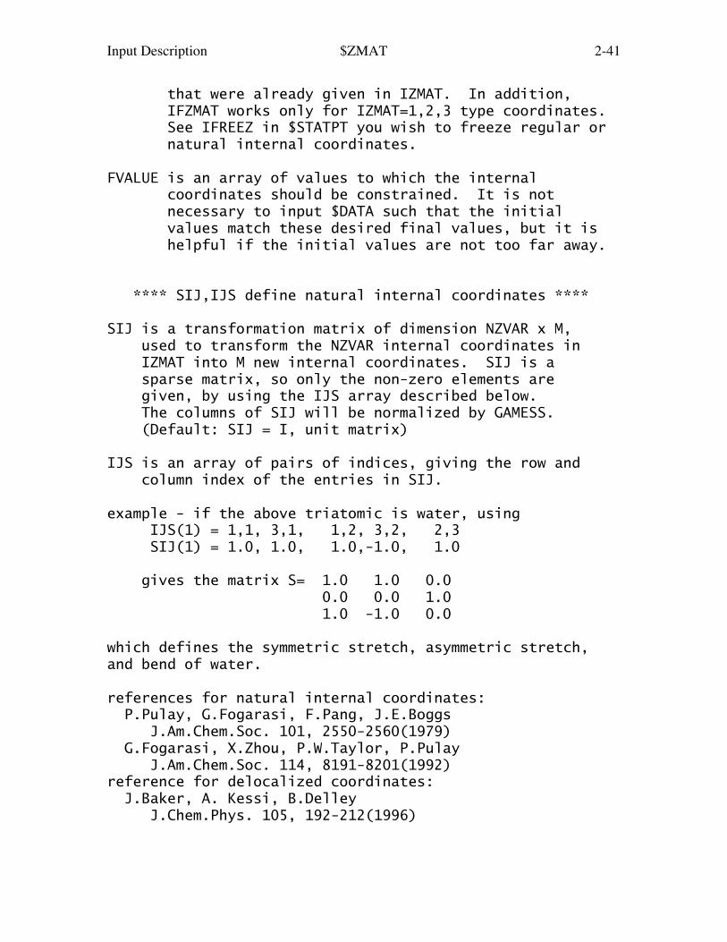
**** SIJ,IJS define natural internal coordinates ****
SIJ is a transformation matrix of dimension NZVAR x M, used to transform the NZVAR internal coordinates in IZMAT into M new internal coordinates. SIJ is a sparse matrix, so only the non-zero elements are given, by using the IJS array described below. The columns of SIJ will be normalized by GAMESS. (Default: SIJ = I, unit matrix)
IJS is an array of pairs of indices, giving the row and column index of the entries in SIJ.
example - if the above triatomic is water, using IJS(1) = 1,1, 3,1, 1,2, 3,2, 2,3 SIJ(1) = 1.0, 1.0, 1.0,-1.0, 1.0
gives the matrix S= 1.0 1.0 0.0 0.0 0.0 1.0 1.0 -1.0 0.0
which defines the symmetric stretch, asymmetric stretch,and bend of water.
references for natural internal coordinates: P.Pulay, G.Fogarasi, F.Pang, J.E.Boggs J.Am.Chem.Soc. 101, 2550-2560(1979) G.Fogarasi, X.Zhou, P.W.Taylor, P.Pulay J.Am.Chem.Soc. 114, 8191-8201(1992)reference for delocalized coordinates: J.Baker, A. Kessi, B.Delley J.Chem.Phys. 105, 192-212(1996)

Input Description $ZMAT 2-42
==========================================================

Input Description $LIBE 2-43
==========================================================
$LIBE group (required if linear bends are used in $ZMAT)
A degenerate linear bend occurs in two orthogonal planes,which are specified with the help of a point A. The firstbend occurs in a plane containing the atoms I,J,K and theuser input point A. The second bend is in the planeperpendicular to this, and containing I,J,K. One suchpoint must be given for each pair of bends used.
APTS(1)= x1,y1,z1,x2,y2,z2,... for linear bends 1,2,...
Note that each linear bend serves as two coordinates, sothat if you enter 2 linear bends (HCCH, for example), thecorrect value of NZVAR is M-2, where M=3N-6 or 3N-5, asappropriate.
==========================================================

Input Description $SCF 2-44
==========================================================
$SCF group relevant if SCFTYP = RHF, UHF, or ROHF, required if SCFTYP = GVB)
This group of parameters provides additional controlover the RHF, UHF, ROHF, or GVB SCF steps. It must begiven to define GVB open shell or perfect pairingwavefunctions. See $MCSCF for multireference inputs.
DIRSCF = a flag to activate a direct SCF calculation, which is implemented for all the Hartree-Fock type wavefunctions: RHF, ROHF, UHF, and GVB. This keyword also selects direct MP2 computation. The default of .FALSE. stores integrals on disk storage for a conventional SCF calculation.
FDIFF = a flag to compute only the change in the Fock matrices since the previous iteration, rather than recomputing all two electron contributions. This saves much CPU time in the later iterations. This pertains only to direct SCF, and has a default of .TRUE. This option is implemented only for the RHF, ROHF, UHF cases. Cases with many diffuse functions in the basis set sometimes oscillate at the end, rather than converging. Turning this parameter off will normally give convergence.
---- The next flags affect convergence rates.
NOCONV = .TRUE. means neither SOSCF nor DIIS will be used. The default is .FALSE., making the choice of the primary converger as follows: for RHF, GVB, UHF, or ROHF (if Abelian): SOSCF for any DFT, or for non-Abelian groups: DIIS.DIIS = selects Pulay's DIIS interpolation.SOSCF = selects second order SCF orbital optimization.
Once either DIIS or SOSCF are initiated, the followingless important accelerators are placed in abeyance:
EXTRAP = selects Pople extrapolation of the Fock matrix.DAMP = selects Davidson damping of the Fock matrix.SHIFT = selects level shifting of the Fock matrix.

Input Description $SCF 2-45
RSTRCT = selects restriction of orbital interchanges.DEM = selects direct energy minimization, which is implemented only for RHF. (default=.FALSE.)
defaults for EXTRAP DAMP SHIFT RSTRCT DIIS SOSCFab initio: T F F F F/T T/Fsemiempirical: T F F F F F
The above parameters are implemented for all SCFwavefunction types, except that DIIS will work for GVB onlyfor those cases with NPAIR=0 or NPAIR=1.
---- These parameters fine tune the various convergers.
CONV = SCF density convergence criteria. Convergence is reached when the density change between two consecutive SCF cycles is less than this in absolute value. One more cycle will be executed after reaching convergence. Less accuracy in CONV gives questionable gradients. The default is 1.0d-05, except runs involving CI or MP2 gradients or CC energies use 1.0d-06.
SOGTOL = second order gradient tolerance. SOSCF will be initiated when the orbital gradient falls below this threshold. (default=0.25 au)
ETHRSH = energy error threshold for initiating DIIS. The DIIS error is the largest element of e=FDS-SDF. Increasing ETHRSH forces DIIS on sooner. (default = 0.5 Hartree)
MAXDII = Maximum size of the DIIS linear equations, so that at most MAXDII-1 Fock matrices are used in the interpolation. (default=10)
SWDIIS = density matrix convergence at which to switch from DIIS to SOSCF. A value of zero means to keep using DIIS at all geometries, which is the default. However, it may be useful to have DIIS work only at the first geometry, in the initial iterations, for example transition metal ECP runs which has a less good Huckel guess, and then use SOSCF for the final SCF

Input Description $SCF 2-46
iterations at the first geometry, and ever afterwards. A suggested usage might be DIIS=.TRUE. ETHRSH=2.0 SWDIIS=0.005. This option is not programmed for GVB.
DEMCUT = Direct energy minimization will not be done once the density matrix change falls below this threshold. (Default=0.5)
DMPCUT = Damping factor lower bound cutoff. The damping damping factor will not be allowed to drop below this value. (default=0.0)note: The damping factor need not be zero to achieve validconvergence (see Hsu, Davidson, and Pitzer, J.Chem.Phys.,65, 609 (1976), see the section on convergence control),but it should not be astronomical either.
* * * * * * * * * * * * * * * * * * * * * For more info on the convergence methods, see the 'Further Information' section. * * * * * * * * * * * * * * * * * * * * *
---- orbital modification options ----
The four options UHFNOS, VVOS, MVOQ, and ACAVO aremutually exclusive. The latter 3 require RUNTYP=ENERGY.
UHFNOS = flag controlling generation of the natural orbitals of a UHF function. (default=.FALSE.)
VVOS = flag controlling generation of Valence Virtual Orbitals. See J.Chem.Phys. 120, 2629-2637(2004).VVOs are a quantitative realization of the concept of"lowest unoccupied orbital" and are also useful for MCSCFstarting orbitals. The implementation at present allowsonly RHF functions, elements up to Xe (excluding transitionmetals), and core potentials may not be used. The defaultis .FALSE. VVOS should be better MCSCF starting orbitalsthan either MVOQ or ACAVO type virtuals.
MVOQ = 0 Skip MVO generation (default) = n Form modified virtual orbitals, using a cation with n electrons removed. Implemented for RHF, ROHF, and GVB. If necessary to reach a closed shell cation, the program might remove

Input Description $SCF 2-47
n+1 electrons. Typically, n will be about 6. = -1 The cation used will have each valence orbital half filled, to produce MVOs with valence-like character in all regions of the molecule. Implemented for RHF and ROHF only.
ACAVO = Flag to request Approximate Correlation-Adapted Virtual Orbitals. Implemented for RHF, ROHF, and GVB. The default is .FALSE.
PACAVO = Parameters used to define the ACAVO generating operator, which is defined as a*T + b*Vne + c*Jcore + d*Jval + e*Kcore + f*KvalThe default corresponds to Whitten orbitals, J.L.Whitten,J.Chem.Phys. 56, 458-546(1972) which maximize the exchangeinteraction with the valence MOs, PACAVO(1)=0,0,0,0,0,-1.0.A set of parameters which may produce a lower CI-SD energy,is 0.02,0.02,0.0,0.10,0.0,-1.0. Of course, the canonicalvirtuals come from PACAVO(1)=1.0,1.0,2.0,2.0,-1.0,-1.0.
----- GVB wavefunction input -----
The next parameters define the GVB wavefunction. Seealso MULT in the $CONTRL group. The GVB wavefunctionassumes orbitals are in the order core, open, pairs.
NCO = The number of closed shell orbitals. The default almost certainly should be changed! (default=0).
NSETO = The number of sets of open shells in the function. Maximum of 10. (default=0)
NO = An array giving the degeneracy of each open shell set. Give NSETO values. (default=0,0,0,...).
NPAIR = The number of geminal pairs in the -GVB- function. Maximum of 12. The default corresponds to open shell SCF (default=0).
CICOEF = An array of ordered pairs of CI coefficients for the -GVB- pairs. (default = 0.90,-0.20,0.90,-0.20,...)
Input Description $SCF 2-48
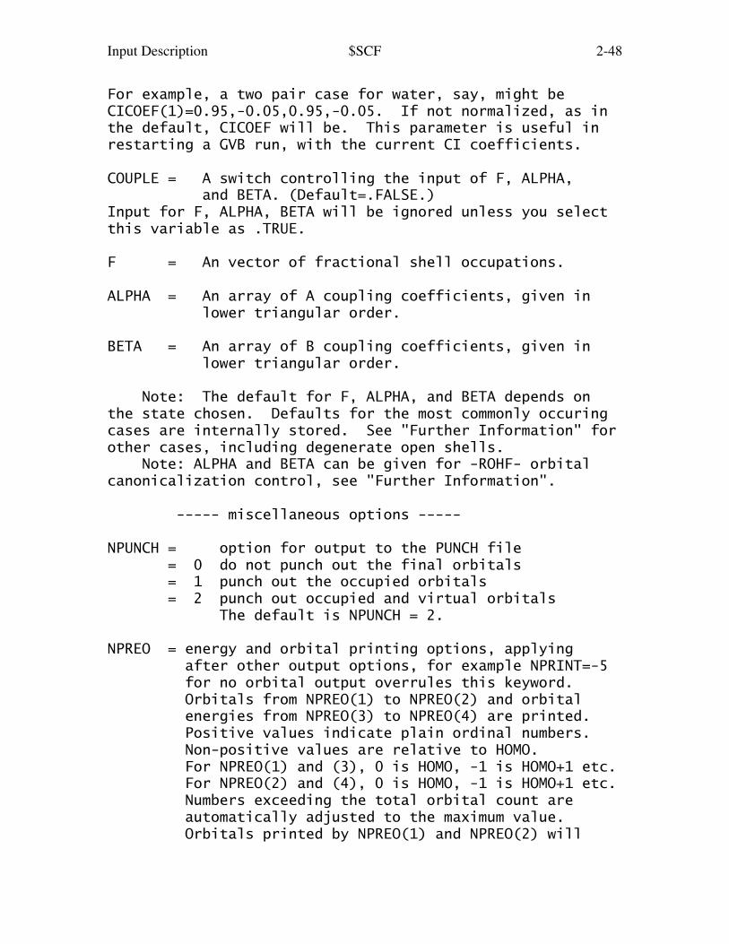
For example, a two pair case for water, say, might beCICOEF(1)=0.95,-0.05,0.95,-0.05. If not normalized, as inthe default, CICOEF will be. This parameter is useful inrestarting a GVB run, with the current CI coefficients.
COUPLE = A switch controlling the input of F, ALPHA, and BETA. (Default=.FALSE.)Input for F, ALPHA, BETA will be ignored unless you selectthis variable as .TRUE.
F = An vector of fractional shell occupations.
ALPHA = An array of A coupling coefficients, given in lower triangular order.
BETA = An array of B coupling coefficients, given in lower triangular order.
Note: The default for F, ALPHA, and BETA depends onthe state chosen. Defaults for the most commonly occuringcases are internally stored. See "Further Information" forother cases, including degenerate open shells. Note: ALPHA and BETA can be given for -ROHF- orbitalcanonicalization control, see "Further Information".
----- miscellaneous options -----
NPUNCH = option for output to the PUNCH file = 0 do not punch out the final orbitals = 1 punch out the occupied orbitals = 2 punch out occupied and virtual orbitals The default is NPUNCH = 2.
NPREO = energy and orbital printing options, applying after other output options, for example NPRINT=-5 for no orbital output overrules this keyword. Orbitals from NPREO(1) to NPREO(2) and orbital energies from NPREO(3) to NPREO(4) are printed. Positive values indicate plain ordinal numbers. Non-positive values are relative to HOMO. For NPREO(1) and (3), 0 is HOMO, -1 is HOMO+1 etc. For NPREO(2) and (4), 0 is HOMO, -1 is HOMO+1 etc. Numbers exceeding the total orbital count are automatically adjusted to the maximum value. Orbitals printed by NPREO(1) and NPREO(2) will
Input Description $SCF 2-49
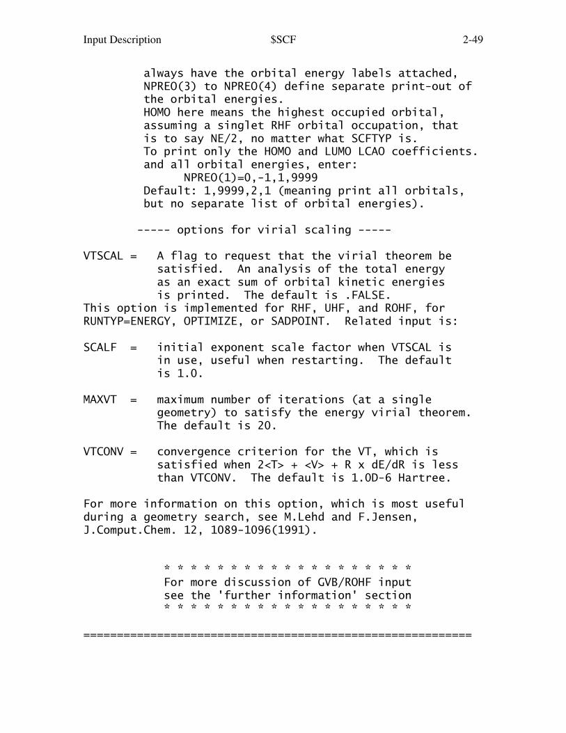
always have the orbital energy labels attached, NPREO(3) to NPREO(4) define separate print-out of the orbital energies. HOMO here means the highest occupied orbital, assuming a singlet RHF orbital occupation, that is to say NE/2, no matter what SCFTYP is. To print only the HOMO and LUMO LCAO coefficients. and all orbital energies, enter: NPREO(1)=0,-1,1,9999 Default: 1,9999,2,1 (meaning print all orbitals, but no separate list of orbital energies).
----- options for virial scaling -----
VTSCAL = A flag to request that the virial theorem be satisfied. An analysis of the total energy as an exact sum of orbital kinetic energies is printed. The default is .FALSE.This option is implemented for RHF, UHF, and ROHF, forRUNTYP=ENERGY, OPTIMIZE, or SADPOINT. Related input is:
SCALF = initial exponent scale factor when VTSCAL is in use, useful when restarting. The default is 1.0.
MAXVT = maximum number of iterations (at a single geometry) to satisfy the energy virial theorem. The default is 20.
VTCONV = convergence criterion for the VT, which is satisfied when 2<T> + <V> + R x dE/dR is less than VTCONV. The default is 1.0D-6 Hartree.
For more information on this option, which is most usefulduring a geometry search, see M.Lehd and F.Jensen,J.Comput.Chem. 12, 1089-1096(1991).
* * * * * * * * * * * * * * * * * * * For more discussion of GVB/ROHF input see the 'further information' section * * * * * * * * * * * * * * * * * * *
==========================================================

Input Description $SCFMI 2-50
==========================================================
$SCFMI group (optional, relevant if SCFTYP=RHF)
The Self Consistent Field for Molecular Interactions(SCF-MI) method is a modification of the usual Roothaanequations that avoids basis set superposition error (BSSE)in intermolecular interaction calculations, by expandingeach monomer's orbitals using only its own basis set.Thus, the resulting orbitals are not orthogonal. Thepresence of a $SCFMI group in the input triggers the useof this option.
The implementation is limited to ten monomers, treatedat the RHF level. The energy, gradient, and thereforesemi-numerical hessian are available. The SCF step may berun in direct SCF mode, and parallel calculation is alsoenabled. The calculation must use Cartesian Gaussian AOsonly, not spherical harmonics. The SCF-MI driver differsfrom normal RHF calculations, so not all converger methodsare available. Finally, this option is not compatible withelectron correlation treatments (DFT, MP2, CI, or CC).
The first 3 parameters must be given. All atoms of afragment must appear consecutively in $DATA.
NFRAGS = number of distinct fragments present. Both the supermolecule and its constituent monomers must be well described as closed shells by RHF wavefunctions.
NF = an array containing the number of doublyoccupied MOs for each fragment.
MF = an array containing the number of atomic basis functions located on each fragment.
ITER = maximum number of SCF-MI cycles, overriding the usual MAXIT value. (default is 50).
DTOL = SCF-MI density convergence criteria. (default is 1.0d-10)
Input Description $SCFMI 2-51
ALPHA = possible level shift parameter. (default is 0.0, meaning shifting is not used)
DIISON = a flag to active the DIIS convergence. (default is .TRUE.)
MXDIIS = the maximum number of previous effective Fockand overlap matrices to be used in DIIS(default=10)
DIISTL = the density change value at which DIIS starts. (default=0.01)
A Huckel guess is localized by the Boys procedure onto eachfragment to provide starting orbitals for each:
ITLOC = maximum number of iteration in the localization step (Default is 50)
CNVLOC = convergence parameter for the localization. (default is .01).
IOPT = prints additional debug information. = 0 standard outout (default) = 1 print for each SCF-MI cycle MOs, overlap between the MOs, CPU times. = 2 print some extra informations in secular systems solution.
==========================================================
"Modification of Roothan Equations to exclude BSSE from Molecular Interaction calculations" E. Gianinetti, M. Raimondi, E. Tornaghi Int. J. Quantum Chem. 60, 157-166 (1996)
"Implementation of Gradient optimization algorithms and Force Constant computations in BSSE-free direct and conventional SCF approaches"
A. Famulari, E. Gianinetti, M. Raimondi, M. Sironi Int. J. Quantum Chem. 69, 151-158 (1997)
Input Description $DFT 2-52
==========================================================
$DFT group (relevant if DFTTYP is chosen) (relevant if SCFTYP=RHF,UHF,ROHF)
Note that if DFTTYP=NONE, an ab initio calculation willbe performed, rather than density functional theory.
This group permits the use of various one electron(usually empirical) operators instead of the true manyelectron Hamiltonian. Two programs are provided, METHOD=GRID or GRIDFREE. The programs have different functionalsavailable, and so the keyword DFTTYP (which is entered in$CONTRL) and other associated inputs are documentedseparately below. Every functional that has the same namein both lists is an identical functional, but each METHODhas a few functionals that are missing in the other.
The grid free implementation is based on the use of theresolution of the identity to simplify integrals so thatthey may be analytically evaluated, without using gridquadratures. The grid free DFT computations in theirpresent form have various numerical errors, primarily inthe gradient vectors. Please do not use the grid-free DFTprogram without reading the discussion in the 'FurtherReferences' section regarding the gradient accuracy.
The grid based DFT uses a typical grid quadrature tocompute integrals over the rather complicated functionals,using two possible angular grid types.
Achieving a self-consistent field with DFT is rathermore difficult than for normal HF, so DIIS is the defaultconverger.
Both DFT programs will run in parallel. See the twolists below for possible functionals in the two programs.
See also the $TDDFT input group for excited states.
METHOD = selects grid based DFT or grid free DFT. = GRID Grid based DFT (default) = GRIDFREE Grid free DFT
Input Description $DFT 2-53
DFTTYP is given in $CONTRL, not here in $DFT! Possiblevalues for the grid-based program are listed first,
----- options for METHOD=GRID -----
DFTTYP = NONE means ab initio computation (default)
Many choices are given below, perhaps the most sensible are local DFT: SVWN pure DFT GGA: BLYP, PW91, B97-D, PBE/PBEsol hybrid DFT GGA: B3LYP, X3LYP, PBE0 pure DFT meta-GGA: TPSS/TPSSm hybrid DFT meta-GGA: TPSSh, M06but of course, everyone has their own favorite!
pure exchange functionals: = SLATER Slater exchange = BECKE Becke 1988 exchange = GILL Gill 1996 exchange = OPTX Handy-Cohen exchange = PW91X Perdew-Wang 1991 exchange = PBEX Perdew-Burke-Ernzerhof exchangeThese will be used with no correlation functional at all.
pure correlation functionals: = VWN Vosko-Wilk-Nusair correlation, using their electron gas formula 5 (VWN5) = VWN1 Vosko-Wilke-Nusair correlation, using their e- gas formula 1, with RPA params. = PZ81 Perdew-Zener 1981 correlation = P86 Perdew 1986 correlation = LYP Lee-Yang-Parr correlation = PW91C Perdew-Wang 1991 correlation = PBEC Perdew-Burke-Ernzerhof correlation = OP One-parameter Progressive correlationThese will be used with 100% HF exchange, if chosen.
combinations (partial list): = SVWN SLATER exchange + VWN5 correlation Called LDA/LSDA in physics for RHF/UHF. = BLYP BECKE exchange + LYP correlation = BOP BECKE exchange + OP correlation = BP86 BECKE exchange + P86 correlation = GVWN GILL exchange + VWN5 correlation
Input Description $DFT 2-54
= GPW91 GILL exchange + PW91 correlation = PBEVWN PBE exchange + VWN5 correlation = PBEOP PBE exchange + OP correlation = OLYP OPTX exchange + LYP correlation = PW91 means PW91 exchange + PW91 correlation = PBE means PBE exchange + PBE correlationThere's a nearly infinite set of pairings (well, 6*8), sowe show only enough to give you the idea. In other words,pairs are formed by abbreviating the exchange functionals SLATER=S, BECKE=B, GILL=G, OPTX=O, PW91X=PW91, PBEX=PBEand matching them with any correlation functional, of whichonly two are abbreviated when used in combinations, PW91C=PW91, PBEC=PBEThe pairings shown above only scratch the surface, butclearly, many possibilities, such as PW91PBE, are nonsense!
pure DFT GGA functionals: = EDF1 empirical density functional #1, which is a modified BLYP from Adamson/Gill/Pople. = PW91 Perdew/Wang 1991 = PBE Perdew/Burke/Ernzerhof 1996 = revPBE PBE as revised by Zhang/Yang = RPBE PBE as revised by Hammer/Hansen/Norskov = PBEsol PBE as revised by Perdew et al for solids = B97-D Grimme's modified B97, with dispersion correction (this forces DC=.TRUE.)
hybrid GGA functionals: = BHHLYP HF and BECKE exchange + LYP correlation = B3PW91 Becke's 3 parameter exchange hybrid, with PW91 correlation functional = B3LYP this is a hybrid method combining five functionals, namely Becke + Slater + HF exchange, and LYP + VWN5 correlation. = B3LYP1 use VWN1 in place of VWN5, matching the e- gas formula chosen by some programs. = B97 Becke's 1997 hybrid functional = B97-1 Hamprecht/Cohen/Tozer/Handy's 1998 reparameterization of B97 = B97-2 Wilson/Bradley/Tozer's 2001 mod to B97 = PBE0 a hybrid made from PBE = X3LYP HF+Slater+Becke88+PW91 exchange, and LYP+VWN1 correlation.Each includes some Hartree-Fock exchange, and also may be alinear combination of many DFT parts.
Input Description $DFT 2-55
meta-GGA functionals:These are not hybridized with HF exchange, unless that isexplicitly stated. = VS98 Voorhis/Scuseria, 1998 = PKZB Perdew/Kurth/Zupan/Blaha, 1999 = TPSS Tao/Perdew/Staroverov/Scuseria, 2003 = TPSSh TPSS hybrid with 10% HF exchange = TPSSm TPSS with modified parameter, 2007 = M05 Minnesota exchange-correlation, 2005 a hybrid with 28% HF exchange. = M05-2X M05, with doubled HF exchange, to 56% = M06 Minnesota exchange-correlation, 2006 a hybrid with 27% HF exchange. = M06-L M06, with 0% HF exchange (L=local) = M06-2X M06, with doubled HF exchange, to 54% = M06-HF M06 correlation, using 100% HF exchangeTruhlar recommends M06 for the general situation, but seehis "concluding remarks" in the M06 reference about whichfunctional is best for what kind of test data set.
An extensive bibliography for these functionals can befound in the 'Further References' section of this manual.
Note that only a subset of these functionals can be usedfor TD-DFT energy or gradients. These subsets are listedin the $TDDFT input group.
DC = a flag to turn on Grimme's empirical dispersion correction, involving scaled R**(-6) terms. Parameters exist for only a few DFTTYP, see DCPAR. (default=.FALSE., except when DFTTYP=B97-D) N.B. This empiricism may also be added to plain Hartree-Fock, by choosing DFTTYP=NONE with DC=.T.
DCOLD = a flag to use Grimme's original 2004 dispersion correction, if you choose DCOLD, you must also set DC on! (default=.FALSE.)
DCPAR = Grimme's parameter S6 for scaling a C6 term added as an empirical correction to otherwise unchanged functionals (showing Grimme's default for S6): BLYP(1.20), PBE(0.75), BP86(1.05), TPSS(1.00), B3LYP(1.05). For B97-D, the DC option will also
Input Description $DFT 2-56
change the original functional, and the scale factor is 1.25. DC works for other functionals, if you make up your own value for DCPAR.
LC = flag to turn on the long range correction (LC), which smoothly replaces the DFT exchange by the HF exchange at long inter-electron distances. (default=.FALSE.) This option can only be used with the Becke exchange functional (Becke) and a few correlation functionals, namely BLYP, BOP, and BVWN, only. For example, B3LYP has a fixed admixture of HF exchange, so it cannot work with the LC option. See H.Iikura, T.Tsuneda, T.Yanai, and K.Hirao, J.Chem.Phys. 115, 3540 (2001).
MU = A parameter for the long range correction scheme. (default=0.33)
* * * Grid Input * * *
Only one of the three grid types may be chosen for the run.The default (if no selection is made) is the Lebedev grid.In order to duplicate results obtained prior to April 2008,select the polar coordinate grid NRAD=96 NTHE=12 NPHI=24.Energies can be compared if and only if the identical gridtype and density is used, analogous to needing to comparewith the identical basis set expansions. See REFS.DOC formore information on grids. See similar inputs in $TDDFT.
Lebedev grid:
NRAD = number of radial points in the Euler-MacLaurin quadrature. (default=96)
NLEB = number of angular points in the Lebedev grids. (default=302). Possible values are 86, 110, 146, 170, 194, 302, 350, 434, 590, 770, 974, 1202, 1454, 1730, 2030...
The default for NLEB means that nuclear gradients will beaccurate to about the default OPTTOL=0.00010 (see $STATPT),590 approaches OPTTOL=0.00001, and 1202 is "army grade".
Input Description $DFT 2-57
The next two specify radial/angular in a single keyword:
SG1 = a flag to select the "standard grid 1", which has 24 radial points, and various pruned Lebedev grids, from 194 down to 6. (default=.FALSE. This grid is very fast, but produces gradients whose accuracy reaches only OPTTOL=0.00050. This grid should be VERY USEFUL for the early steps of a geometry optimization.
JANS = two unpublished grids due to Curtis Janssen, implemented here differently than in MPQC: = 1 uses 95 radial points for all atoms, and prunes from a Lebedev grid whose largest size is 434, thus using about 15,000 grid points/atom. = 2 uses 155 radial points for all atoms, and prunes from a Lebedev grid whose largest size is 974, thus using about 71,000 grid points/atom. This is a very accurate grid, e.g. "army grade".
polar coordinate grid:
NRAD = number of radial points in the Euler-MacLaurin quadrature. (96 is reasonable)
NTHE = number of angle theta grids in Gauss-Legendre quadrature (polar coordinates). (12 is reasonable)
NPHI = number of angle phi grids in Gauss-Legendre quadrature. NPHI should be double NTHE so points are spherically distributed. (24 is reasonable)
The number of angular points will be NTHE*NPHI. The valuesshown give a gradient accuracy near the default OPTTOL of0.00010, while NTHE=24 NPHI=48 approaches OPTTOL=0.00001,and "army grade" is NTHE=36 NPHI=72.
* * * Grid Switching * * *
At the first geometry of the run, pure HF iterations willbe performed, since convergence of DFT is greatly improvedby starting with the HF density matrix. After DFT engages,most runs (at all geometries, except for PCM or numerical
Input Description $DFT 2-58
Hessians) will use a coarser grid during the early DFTiterations, before reaching some initial convergence.After that, the full grid will be used. Together, theseswitchings can save considerable CPU time.
SWOFF = turn off DFT, to perform pure SCF iterations, until the density matrix convergence falls below this threshold. This option is independent of SWITCH and can be used with or without it. It is reasonable to pick SWOFF > SWITCH > CONV in $SCF. SWOFF pertains only to the first geometry that the run computes, and is automatically disabled if you choose GUESS=MOREAD to provide initial orbitals. The default is 5.0E-3.
SWITCH = when the change in the density matrix between iterations falls below this threshhold, switch to the desired full grid (default=3.0E-4) This keyword is ignored if the SG1 grid is used.
NRAD0 = same as NRAD, but defines initial coarse grid. default = smaller of 24 and NRAD/4
NLEB0 = same as NLEB, but defines initial coarse grid. default = 110
NTHE0 = same as NTHE, but defines initial coarse grid. default = smaller of 8, NTHE/3
NPHI0 = same as NPHI, but defines initial coarse grid. default = smaller of 16, NPHI/3
technical parameters:
THRESH = threshold for ignoring small contributions to the Fock matrix. The default is designed to produce no significant energy loss, even when the grid is as good as "army grade". If for some reason you want to turn all threshhold tests off, of course requiring more CPU, enter 1.0e-15. default: 1.0e-4/Natoms/NRAD/NTHE/NPHI
GTHRE = threshold applied to gradients, similar to THRESH. < 1 assign this value to all thresholds

Input Description $DFT 2-59
= 1 use the default thresholds (default). > 1 divide default thresholds by this value. If you wish to increase accuracy, set GTHRE=10. The default introduces an error of roughly 1e-7 (a.u./bohr) in the gradient.
Input Description $DFT 2-60
The keyword $DFTTYP is given in $CONTRL, and may have thesevalues if the grid-free program is chosen:
----- options for METHOD=GRIDFREE -----
DFTTYP = NONE means ab initio computation (default) exchange functionals: = XALPHA X-Alpha exchange (alpha=0.7) = SLATER Slater exchange (alpha=2/3) = BECKE Becke's 1988 exchange = DEPRISTO Depristo/Kress exchange = CAMA Handy et al's mods to Becke exchange = HALF 50-50 mix of Becke and HF exchange correlation functionals: = VWN Vosko/Wilke/Nusair correlation, formula 5 = PWLOC Perdew/Wang local correlation = LYP Lee/Yang/Parr correlation exchange/correlation functionals: = BVWN Becke exchange + VWN5 correlation = BLYP Becke exchange + LYP correlation = BPWLOC Becke exchange + Perdew/Wang correlation = B3LYP hybrid HF/Becke/LYP using VWN formula 5 = CAMB CAMA exchange + Cambridge correlation = XVWN Xalpha exchange + VWN5 correlation = XPWLOC Xalpha exchange + Perdew/Wang correlation = SVWN Slater exchange + VWN5 correlation = SPWLOC Slater exchange + PWLOC correlation = WIGNER Wigner exchange + correlation = WS Wigner scaled exchange + correlation = WIGEXP Wigner exponential exchange + correlation
AUXFUN = AUX0 uses no auxiliary basis set for resolution of the identity, limiting accuracy. = AUX3 uses the 3rd generation of RI basis sets, These are available for the elements H to Ar, but have been carefully considered for H-Ne only. (DEFAULT)
THREE = a flag to use a resolution of the identity to turn four center overlap integrals into three center integrals. This can be used only if no auxiliary basis is employed. (default=.FALSE.)==========================================================
Input Description $TDDFT 2-61
==========================================================
$TDDFT group (relevant if TDDFT chosen in $CONTRL)
This group generates molecular excitation energies bytime-dependent density functional theory computations (ortime-dependent Hartree-Fock, also known as the Random PhaseApproximation). The functional used for the excited statesis necessarily the same one that is used for the groundstate, specified by DFTTYP in $CONTRL. Analytic gradientsare available for singlet excited states, while the energyof excited states of other multiplicities can be computed.Excited state properties are calculated using the TDDFTexcited state electronic density only during gradient runs.See the "limitations" below regarding available gradientsand solvent models.
Permissible values for DFTTYP are NONE - use TDHF (i.e. Random Phase Approximation),noting that extra states may need to be solved for in orderto be sure of getting the first few states correctly. Youmay also choose any of the following functionals: SVWN, SOP, SLYP, BVWN, BOP, BLYP, OLYP, B3LYP, PBE, PBE0, or NONEwhen computing the gradient of an excited state. Forevaluation of excitation energies, you may use SVWN, SVWN1, SPZ81, SP86, SOP, SLYP, BVWN, BVWN1, BPZ81, BP86, BOP, BLYP, OLYP, B3LYP, B3LYP1, B3PW91, X3LYP, PBE, PBE0, or NONE.
The LC flag in $DFT also pertains to TDDFT runs. The LCoption may be used with the "B" functionals, and isnormally very useful in obtaining better descriptions forcharge-transfer excitations or Rydberg excitation energiesthan are conventional exchange correlation functionals(whether pure or hybrid). The LC flag is also availablefor excited state gradient computation.
TDDFT is a single excitation theory. All of the caveatslisted in the $CIS input group about states with doubleexcitation character, need for Rydberg basis sets, greatlydifferent topology of excited state surfaces, and so onapply here as well. Please read the introduction to the
Input Description $TDDFT 2-62
$CIS input group! If you use very large or very smallGaussian exponents, you may need to increase the number ofradial grid points (the program prints advice in suchcases).
TDHF, TDDFT, and CIS are related in the following way: -- Tamm/Dancoff approximation --> | TDHF CIS DFT | V TDDFT TDDFT/TDAwith only the lower right corner not being possible withGAMESS. Note also that here TDHF means absorption ofphotons, to produce excited states. This should not beconfused with the photon scattering processes computed byRUNTYP=TDHF or TDHFX, which generate polarizabilities.
Parallel computation is enabled.
Limitations:
For SCFTYP=RHF, excitation energies can be found forsinglet or triplet coupled excited states. For singletexcited states, analytic gradients and properties can befound. For RHF references, excited state energy runs canincorporate solvent effects using EFP1 (specifically, theH2ODFT potential), or using C-PCM (IEF=-10). Unlike theground state, it is not possible to combine EFP with PCM.
For SCFTYP=UHF, excited state energies for states of thesame spin multiplicity as the ground state can be found.There are no properties (other than the excitation energy),nor gradients, nor solvent effects, at the present time.
NSTATE = Number of states to be found (excluding the ground state). The default is 1 more state.
IROOT = State used for geometry optimization and property evaluation. (default=1, the 1st excited state)
MULT = Multiplicity (1 or 3) of the singly excited states. This keyword applies only when the reference is a closed shell. (default is 1)
TDPRP = a flag to request property computation for the
Input Description $TDDFT 2-63
state IROOT. This requires significant extra computer time, compared to the excitation energy alone, so the default is .FALSE. Properties are always evaluated during nuclear gradient runs, when they are a free by-product. This option is only available for RHF references, and MULT=1.
NONEQ is a flag controlling PCM's solvent behavior: .TRUE. splits the dielectric constant into a bulk value (EPS in $PCM) and a fast component (EPSINF), see Cossi and Barone, 2001. The idea is that NONEQ=.t. is appropriate for vertical excitations, and .f. for adiabatic. (the default is .TRUE.)
* * * Grid Selection * * *
The grid type and point density used in $TDDFT may bechosen independently of the values in $DFT. Excitationenergies accurate to 0.01 eV may be obtained with gridsthat are much sparser than those needed for the groundstate, and this is reflected in the defaults. Prior toApril 2008, the default grid was NRAD=24 NTHE=8 NPHI=16.
NRAD = number of radial grid points in Euler-Maclaurin quadrature, used in calculations of the second or third derivatives of density functionals. (default=48)
NLEB = number of angular points in the Lebedev grid. (default=110)
NTHE = number of theta grid points if a polar coordinate grid is used.
NPHI = number of phi grid points if a polar coordinate grid is used. NPHI should be twice NTHE.
SG1 = flag selecting "standard grid one". (default=.FALSE.)
See both $DFT and REFS.DOC for more information on grids.The "army grade" standard for $TDDFT is NRAD=96 combinedwith either NLEB=302 or NTHE=12/NPHI=24.
Input Description $TDDFT 2-64
the remaining parameters are technical in nature:
CNVTOL = convergence tolerance in the iterative TD-DFT step. (default=1.0E-7)
MAXVEC = the maximum number of expansion vectors used by the solver's iterations, per state (default=50). The total size of the expansion space will be NSTATE*MAXVEC.
NTRIAL = the number of initial expansion vectors used. (default is the larger of 5 and NSTATE).
==========================================================
Input Description $CIS 2-65
==========================================================
$CIS group required when CITYP=CIS
The CIS method (singly excited CI) is the simplest wayto treat excited states. By Brillouin's Theorem, a singledeterminant reference such as RHF will have zero matrixelements with singly substituted determinants. The groundstate reference therefore has no mixing with the excitedstates treated with singles only. Reading the referencesgiven in Section 4 of this manual will show the CIS methodcan be thought of as a non-correlated method, rigorously sofor the ground state, and effectively so for the variousexcited states. Some issues making CIS rather less than ablack box method are: a) any states characterized by important doubles are simply missing from the calculation. b) excited states commonly possess Rydberg (diffuse) character, so the AO basis used must allow this. c) excited states often have different point group symmetry than the ground state, so the starting geometries for these states must reflect their actual symmetry. d) excited state surfaces frequently cross, and thus root flipping may very well occur.The implementation allows the use of only RHF references,but can pick up both singlet and triplet excited states.Nuclear gradients are available, as are properties. TheCIS run automatically includes computation of the dipolemoments of all states, and all pairwise transition dipolesand oscillator strengths.
NACORE = n Omits the first n occupied orbitals from the calculation. The default for n is the number of chemical core orbitals.
NSTATE = Number of states to be found (excluding the ground state, which is the RHF determinant).
IROOT = State for which properties and/or gradient will be calculated. Only one state can be chosen.
HAMTYP = Type of CI Hamiltonian to use. = SAPS spin-adapted antisymmetrized product of the desired MULT will be used (default) = DETS determinant based, so both singlets and

Input Description $CIS 2-66
triplets will be obtained.
MULT = Multiplicity (1 or 3) of the singly excited SAPS (the reference is necessarily single RHF). Only relevant for SAPS based run.
DIAGZN = Hamiltonian diagonalization method. = DAVID use Davidson diagonalization. (default) = FULL construct the full matrix in memory and diagonalize, thus determining all states (not recommended except for small cases).
DGAPRX = Flag to control whether approximate diagonal elements of the CIS Hamiltonian (based only on the orbital energies) are used in the Davidson algorithm. Note, this only affects the rate of convergence, not the resulting final energies. If set .FALSE., the exact diagonal elements are determined and used. Default=.TRUE.
NGSVEC = Dimension of the Hamiltonian submatrix that is diagonalized to form the initial CI vectors. The default is the greater of NSTATE*2 and 10.
MXVEC = Maximum number of expansion basis vectors in the iterative subspace during Davidson iterations, before the expansion basis is truncated. The default is the larger of 8*NSTATE and NGSVEC.
NDAVIT = Maximum number of Davidson iterations. Default=50.
DAVCVG = Convergence criterion for Davidson eigenvectors. Eigenvector accuracy is proportional to DAVCVG, while the energy accuracy is proportional to its square. The default is 1.0E-05.
CISPRP = Flag to request the determination of CIS level properties, using the relaxed density. Relevant to RUNTYP=ENERGY jobs, although the default is .FALSE. because additional CPHF calculation will be required. Properties are a normal by product of runs involving the CIS gradient.
CHFSLV = Chooses type of CPHF solver to use.
Input Description $CIS 2-67
= CONJG selects an ordinary preconditioned conjugate gradient solver. (default) = DIIS selects a diis-like iterative solver.
RDCISV = Flag to read CIS vectors from a $CISVEC group in the input file. Default is .FALSE.
MNMEDG = Flag to force the use of the minimal amount of memory in construction of the CIS Hamiltonian diagonal elements. This is only relevant when DGAPRX=.FALSE., and is meant for debug purposes. The default is .FALSE.
MNMEOP = Flag to force the use of the minimal amount of memory during the Davidson iterations. This is for debug purposes. The default is .FALSE.
==========================================================
$CISVEC group required if RDCISV in $CIS is chosen
This is formatted data generated by a previous CIS run, tobe read back in as starting vectors. Sometimes molecularorbital phase changes make these CI vectors problematic.==========================================================
Input Description $MP2 2-68
==========================================================
$MP2 group (relevant to SCFTYP=RHF,UHF,ROHF if MPLEVL=2)
Controls 2nd order Moller-Plesset perturbation runs,if requested by MPLEVL in $CONTRL. MP2 is implemented forRHF, high spin ROHF, or UHF wavefunctions, but see also$MRMP for MCSCF. Analytic gradients and the first ordercorrection to the wavefunction (i.e. properties) areavailable for RHF, ROHF (if OSPT=ZAPT), and UHF. The $MP2group is not usually given. See also the DIRSCF keyword in$SCF to select direct MP2.
The spin-component-scaled MP2 (SCS-MP2) energy ofGrimme is printed for SCFTYP=RHF references during CODE=IMSor SERIAL energy runs, also, see keyword SCSPT below.
Special serial codes exist for RHF or UHF MP2 energyor gradient, or the ROHF MP2 energy. Parallel codes usingdistributed memory are available for RHF, ROHF, or UHF MP2gradients. In fact, the only way that ROHF MP2 gradientscan be computed on one node is with the parallel code,using MEMDDI!
NACORE = n Omits the first n occupied orbitals from the calculation. The default for n is the number of chemical core orbitals.
NBCORE = Same as NACORE, for the beta orbitals of UHF. It is almost always the same value as NACORE.
MP2PRP= a flag to turn on property computation for jobs jobs with RUNTYP=ENERGY. This is appreciably more expensive than just evaluating the second order energy correction alone, so the default is to skip properties. Properties are always computed during gradient runs, when they are an almost free byproduct. (default=.FALSE.)
OSPT= selects open shell spin-restricted perturbation. This parameter applies only when SCFTYP=ROHF. Please see the 'further information' section for more information about this choice. = ZAPT picks Z-averaged perturbation theory. (default) = RMP picks RMP (aka ROHF-MBPT) perturbation theory.

Input Description $MP2 2-69
CODE = the program implementation to use, choose from SERIAL, DDI, or IMS according to the following chart, depending on SCFTYP and if the run involves gradients,
RHF RHF UHF UHF ROHF ROHF ROHFenergy gradient energy gradient energy gradient energy OSPT=ZAPT ZAPT RMPSERIAL SERIAL SERIAL SERIAL SERIAL - SERIALDDI DDI DDI DDI DDI DDI -IMS IMS - - - - -
The default is CODE=SERIAL when p=1, provided PARALL is.FALSE. in $SYSTEM. When p>1, or PARALL=.TRUE., thedefault becomes CODE=DDI. However, if FMO is in use, thedefault for parallel runs is CODE=IMS. The "SERIAL" codefor OSPT=RMP will run with modest scalability when p>1.
The three programs are written for different hardwaresituations. Here N is the number of atomic basisfunctions, and O is the number of correlated orbitals inthe run:
The SERIAL program uses N**3 memory, but has much smallerdisk files, and generally takes longer than CODE=IMS.
The IMS program uses N*O**2 memory, and places most of itsdata on local disks (so you must have good disk access),and will run in parallel...ideal for PC clusters.
The DDI program uses N**4 memory, but this is distributedacross all nodes, and there is essentially no I/O...idealfor large parallel machines where the manufacturer hasforgotten to include disk drives. MEMDDI must be given forthese codes.
References for these programs are given in REFS.DOC.
NOSYM = disables the orbital symmetry test completely. This is not recommended, as loss of orbital symmetry is likely to mean a bad calculation. It has the same meaning as the keyword in $CONTRL, but just for the MP2 step. (Default=0)

Input Description $MP2 2-70
CUTOFF = transformed integral retention threshold, the default is 1.0d-9 (1.0d-12 in FMO runs).
The following keyword can only be used during CODE=IMSclosed shell runs (energy or gradient):
SCSPT = spin component scaled MP2 energy selection. This energy is printed during CODE=IMS energy or gradient runs, and by CODE=SERIAL energy runs. = NONE - the energy will be the normal MP2 value. = SCS - the energy used for the potential surface will be the SCS energy value. The default is NONE.
The following keywords apply to any CODE=SERIAL MP2 run, orto parallel ROHF+MP2 runs using OSPT=RMP:
LMOMP2= a flag to analyze the closed shell MP2 energy in terms of localized orbitals. Any type of localized orbital may be used. This option is implemented only for RHF, and its selection forces use of the METHOD=3 transformation, in serial runs only. The default is .FALSE.
CPHFBS = BASISMO solves the response equations during gradient computations in the MO basis. This is programmed only for RHF references without frozen core orbitals, when it is the default. = BASISAO solves the response equations using AO integrals, for frozen core MP2 with a RHF reference, or for ROHF or UHF based MP2.
NWORD = controls memory usage. The default uses all available memory. Applies to CODE=SERIAL. (default=0)
METHOD= n selects transformation method, 2 being the segmented transformation, and 3 being a more conventional two phase bin sort implementation. 3 requires more disk, but less memory. The default is to attempt method 2 first, and method 3 second. Applies only to CODE=SERIAL.
AOINTS= defines AO integral storage during conventional integral transformations, during parallel runs.

Input Description $MP2 2-71
DUP stores duplicated AO lists on each node, and is the default for parallel computers with slow interprocessor communication, e.g. ethernet. DIST distributes the AO integral file across all nodes, and is the default for parallel computers with high speed communications. Applies only to parallel OSPT=RMP runs.
==========================================================

Input Description $CCINP 2-72
==========================================================
$CCINP group (optional, relevant for any CCTYP)
This group controls a coupled-cluster calculation ofany type specified by CCTYP in $CONTRL. The referenceorbitals may be RHF or high spin ROHF. If this input groupis not given, as is usually the case, all valence electronswill be correlated.
Excited state runs CCTYP=EOM-CCSD or CR-EOM also readthis group to define the orbitals and to control the groundstate CCSD step that preceeds computation of excitations.Excitation energies are possible only for a RHF reference.
Parallel computation is possible for RHF referencesonly, and only for CCTYP=CCSD or CCSD(T). Memory use inparallel runs is exotic, be certain to use EXETYP=CHECK (onone processor, with PARALL in $SYSTEM set) before running.
See the "Further Information" section of this manualfor more details.
The first four inputs pertain to both RHF and ROHF cases:
NCORE = gives the number of frozen core orbitals to be omitted from the CC calculation. The default is the number of chemical core orbitals.
NFZV = the number of frozen virtual orbitals to be omitted from the calculation. (default is 0)
MAXCC = defines the maximum number of CCSD (or LCCD, CCD) iterations. This parameter also applies to ROHF's left CC vector solver, but not RHF's left vector. See MAXCCL for RHF. (default=30)
ICONV = defines the convergence criterion for the cluster amplitudes, as 10**(-ICONV). The ROHF reference also uses this for its left eigenstate solver, but see CVGEOM in $EOMINP for RHF references. (default is 7, but it tightens to 8 for FMO-CC.)

Input Description $CCINP 2-73
**** the next group pertains to RHF reference only ****
CCPRP = a flag to select computation of the CCSD level ground state density matrix (see also CCPRPE in $EOMINP for EOM-CCSD level excited states). The computation takes significant extra time, to obtain left eigenstates, so the default is .FALSE. except for CCTYP=CR-CCL where the work required for properties must be done anyway.
Notes: CCSD is the only level at which properties can beobtained. Therefore this option can only be chosen forCCTYP=CCSD, CR-CCL, EOM-CCSD, or CR-EOM. The run willchange CCTYP to EOM-CCSD if you choose CCSD, and willtherefore read $EOMINP. However, if you don't selectNSTATE in $EOMINP, your original CCTYP=CCSD will notinclude anything except the ground state in the EOM-CCSD.Note that the convergence criterion for left eigenstateswill be CVGEOM in $EOMINP, which is set to obtainexcitation energies, and may need tightening. Use ofCCTYP=CR-EOM will do triples corrections, after doing theSD level properties.
There is little reason to select any of these:
MAXCCL = iteration limit on the left eigenstate needed by CCSD properties, or CR-CCL energies. This is just a synonym for MAXEOM in $EOMINP. If you want to alter the left state's convergence tolerance, use CVGEOM in $EOMINP. The right state convergence is set by MAXCC and ICONV above.
NWORD = a limit on memory to be used in the CC steps. The default is 0, meaning all memory available will be used.
IREST = defines the restart option. If the value of IREST is greater or equal 3, program will restart from the earlier CC run. This requires saving the disk file CCREST from the previous CC run. Values of IREST between 0 and 3 should not be used. In general, the value of IREST is used by the program to set the iteration counter in the restarted run.
Input Description $CCINP 2-74
The default is 0, meaning no restart is attempted.
MXDIIS = defines the number of cluster amplitude vectors from previous iterations to be included in the DIIS extrapolation during the CCSD (or LCCD, CCD) iterative process. The default value of MXDIIS is 5 for all but small problems. The DIIS solver can be disengaged by entering MXDIIS = 0. It is not necessary to change the default value of MXDIIS, unless the CC equations do not converge in spite of increasing the value of MAXCC.
AMPTSH = defines a threshold for eliminating small cluster amplitudes from the CC calculations. Amplitudes with absolute values smaller than AMPTSH are set to zero. The default is to retain all small amplitudes, meaning fully accurate CC iterations. Default = 0.0.
**** the next group pertains to ROHF reference only **** There is little reason to select any of these.
MULT = spin multiplicity to use in the CC computation. The value of MULT given in the $CONTRL group determines the spin state for the ROHF reference orbitals, and is the default for the CC step.
IOPMET = method for the CR-CC(2,3) triples correction. = 0 means try 1 and then try 2 (default) = 1, the high memory option This option uses the most memory, but the least disk storage and the least CPU time. = 2, the high disk option This option uses least memory, by storing a large disk file. Time is slightly more than IOPMET=1, but the disk file is (NO**3 * NU**3)/6 words, where NO = correlated orbitals, and NU= virtuals. = 3, the high I/O option This option requires slightly more memory than 2, and slightly more disk than 1, but does much I/O. It is also the slowest of the three choices.Check runs will print memory needed by all three options.
Input Description $CCINP 2-75
KREST = 0 fresh start of the CCSD equations (default) = 1 restart from AMPROCC file of a previous run
KMICRO = n performs DIIS extrapolation of the open shell CCSD, every n iterations (default is 6) Enter 0 to avoid using the DIIS converger.
LREST = 0 fresh start of the left CCSD equations (default) = 1 restart from AMPROCC file of a previous run
LMICRO = n performs DIIS extrapolation of the open shell left equations, every n iterations (default is 5) Enter 0 to avoid using the DIIS converger. KMICRO and LMICRO are ignored for trivial problem sizes.
==========================================================
Input Description $EOMINP 2-76
==========================================================
$EOMINP group (optional, for CCTYP=EOM-CCSD or CR-EOM) (optional for CCSD properties, or CCTYP=CR-CCL)
This group controls the calculation of excited statesby the equation of motion coupled cluster with single anddouble excitations, with optional triples corrections. Theinput group permits selection of how many states arecomputed (machine time is linear in the number of states).Since the default is only one excited state in the totallysymmetric representation, it is usually necessary to givethis group. The input also allows selection of variouscomputational procedures.
An excited state coupled cluster run consists of an RHFcalculation, followed by a ground state CCSD (see the$CCINP group to control the ground state calculation, andthe orbital range correlated), followed by an EOM-CCSDcalculation. If CCTYP=CR-EOM, triples corrections based onthe method of moments approach may follow these steps.
The various types of triples corrections mentionedbelow, and other information, can be found in the "FurtherInformation" section of this manual.
--- state symmetry and state selection:
GROUP the name of the Abelian group to be used, which may be only one of the groups shown in the table below. The default is taken from $DATA, and is reset to C1 if the group is non-Abelian. The purpose is to let the Abelian symmetry be turned off by setting GROUP=C1, if desired. Symmetry is used to help with the initial excited state selection, for controlling the EOMCC calculations, and for labeling the calculated states in the output (not to speed up the calculations).
NSTATE an array of up to 8 integers telling how many singlet excited states of each symmetry type should be computed. The default is NSTATE(1)=1,0,0,0,0,0,0,0 which means 1 excited

Input Description $EOMINP 2-77
totally symmetric singlet state is to be found. The ground state, which must lie in the totally symmetric irrep due to use of an RHF reference is always computed, and therefore should NOT be included in the number of totally symmetric excited states requested. There is no particular reason to think the first excited state will be totally symmetric, so most runs should give NSTATE input. Up to 10 states can be found in any irrep. Machine time is linear in the number of states to be found, so be realistic about how many states you solve for (particularly, with multi-root solvers). The choice of NSTATE(1)=0,0,0,0,0,0,0,0 means calculating the ground state only, yielding the new types of ground-state CR-CCSD(T) corrections labeled as types I, II, and III (see MTRIP).
irreducible representation symmetry table: irrep 1 2 3 4 5 6 7 8 C1 A C2 A B Cs A' A'' Ci Ag Au C2v A1 A2 B1 B2 C2h Ag Au Bg Bu D2 A B1 B2 B3 D2h Ag Au B1g B1u B2g B2u B3g B3u Note that this differs from $DET, $MCQDPT, etc!
IROOT selects the state whose energy is to be saved for further calculations (default IROOT(1)=1,0). The first integer lists the irrep number, from the same table as NSTATE. The second lists the number of the excited state. The default corresponds to the ground state (labeled as state 0), as this state must lie in the totally symmetric representation. IROOT(1)=3,2 means the second excited state of symmetry B1, if the if the point group is C2v. The energy of the state selected is stored as the energy used for numerical derivative calculation, TRUDGE, etc. The energy saved will be the EOMCCSD value unless the triples correction are obtained, in which case the type III energy will be saved (if available) or else the type
Input Description $EOMINP 2-78
ID energy. If degenerate states are present, triples are evaluated for only one such state, namely the one with lower irrep number. The EOM-CCSD energies will be used to map an IROOT for a higher irrep number to this, but if the triples corrections alter the order of the states, the new IROOT may not pick up the state you are interested in. Fixes: pick the lower irrep number, or request states only in one symmetry type.
CCPRPE = a flag to select computation of the EOM-CCSD level excited state density matrices (see also CCPRP in $CCINP for ground states). The computation takes extra time, to obtain left eigenstates, so the default is .FALSE.
Note: CCPRPE will evaluate excited states' dipole moments,and the transition moments and oscillator strengths betweenall states. This option can be chosen for CCTYP=EOMCCSD orCR-EOM, with the latter doing triples corrections after theSD level properties are obtained. Selecting this option,or CCPRP in $CCINP, requires extra time due to solving forthe left eigenvectors (from the so-called "lambda"equation). CVGEOM will affect the accuracy of the computedproperties. The resulting density matrices are square, notsymmetric, and at present cannot be used for any propertyother than the dipole quantities. As a temporaryexpedient, they are output in the PUNCH file for possibleuse elsewhere.
--- methods of converging the EOMCCSD equations and selecting triples corrections to EOMCCSD energies:
MEOM selects the solver for the EOMCCSD calculations: 0 = one EOMCCSD root at a time, united iterative space for all calculated roots (default) 1 = one root at a time, separate iterative space for each calculated root 2 = the Hirao-Nakatsuji multi-root solver 3 = one root at a time, separate iterative space for all computed right/left roots. (compare to 1) 4 = one root at a time, united iterative spaces for each right/left root (compare to 0).

Input Description $EOMINP 2-79
MEOM=0,1,2 obtain all the right eigenvectors first, andthen if properties are being computed, proceed to computethe left eigenvectors. MEOM=3,4 obtain right and lefteigenvectors simultaneously, and therefore should only bechosen if you are computing properties (see CCPRP/CCPRPE).
the next two apply only to CCTYP=CR-EOM:
MTRIP selects the type of noniterative triples corrections to EOMCCSD energies: 1 = compute the CR-EOMCCSD(T) triples corrections termed type I and II in the output. This is the default, which skips the iterative CISD calculations needed to construct the CR-EOMCCSD(T) triples corrections of type III. 2 = after performing an additional CISD calculation, evaluate all types of the CR-EOMCCSD(T) triples corrections, including types I, II, and III. This choice of MTRIP uses approximately 50 % more memory, but less CPU time than MTRIP=4. 3 = evaluate the CR-EOMCCSD(T) corrections of type III only. As with MTRIP=2, this calculation includes the iterative CISD calculation, which is needed to construct the type III triples corrections, in addition to the EOMCCSD and CR-EOMCCSD(T) calculations. 4 = carry out MTRIP=1 calculations, followed by MTRIP=3 calculations, thus evaluating all types of the CR-EOMCCSD(T) corrections (types I, II, and III in the output). As with MTRIP=2, this calculation includes the CISD iterations, which are needed to construct the type III triples corrections, in addition to the EOMCCSD and CR-EOMCCSD(T) calculations. Compared to MTRIP=2, this choice of MTRIP uses less memory, but more CPU time.
MCI selects the solver for the CISD step, which is irrelevant unless MTRIP is bigger than 1. 1 = one root at a time, separate iterative space for each calculated root (default) 2 = the Hirao-Nakatsuji multi-root solver (slower)
--- initial guess for the EOMCCSD and possible CISD steps:
Input Description $EOMINP 2-80
MINIT selects the initial guess procedure for both the EOMCCSD and CISD iterations (when MTRIP>1). 1 = (not a default, but HIGHLY RECOMMENDED). Use EOMCCSd to start the EOMCCSD iterations and use CISd to start the CISD iterations during the CR-EOMCCSD(T), type III, calculations. This means that the initial guesses for the calculated states are defined using all single excitations (letter S in EOMCCSd and CISd) and a small subset of double excitations (the little d in EOMCCSd and CISd) defined by active orbitals or orbital range specified by the user. The inclusion of a small set of active doubles in addition to all singles in the initial guess facilitates finding excited states characterized by relatively large doubly excited amplitudes. This choice of MINIT is strongly recommended. (see NOACT, NUACT, and MOACT). 2 = Use CIS wave functions as initial guesses for the EOMCCSD and possible CISD calculations. This is the default, but may cause severe convergence difficulties or even miss some states entirely if the calculated states have significant doubly excited character. MINIT=1 is much better in these situations and strongly recommended, particularly when there is a chance of having low-lying states with nonnegligible bi-excited or multi-configurational character.
the next three apply only to MINIT=1:
NOACT the number of occupied MOs in the active space for the EOMCCSd and CISd initial guesses.NUACT the number of unoccupied MOs in the active space for the EOMCCSd and CISd initial guesses. The NOACT and NUACT variables are used only by MINIT=1, and are reset to 0 if MINIT=2. There are no default values of NOACT and NUACT and the user MUST provide NOACT and NUACT values when MINIT=1. The values of NOACT and NUACT should be small (5 or so), since they only describe the numbers of highest-energy occupied and lowest-energy unoccupied MOs that should help to capture the leading orbital excitations

Input Description $EOMINP 2-81
defining the excited states of interest (see an example below). The user should make sure that the active orbital range defined by NOACT and NUACT does not fall across degenerate orbitals (e.g., if NUACT is chosen such that only one of the two degenerate pi orbitals is included in the active orbital range for the EOMCCSd and CISd initial guesses, the user should increase NUACT at least by 1 to make sure that both pi orbitals are included in the active orbital set). See also the MOACT input for fine tuning.MOACT array allowing explicit selection of the active orbitals used to define the EOMCCSd and CISd initial guesses. If not provided, the MOACT array is filled such that the NOACT highest occupied and NUACT lowest unoccupied orbitals are selected. If MOACT array is given, the number of values in it must equal NOACT+NUACT. Sometimes, instead of defining larger NUACT values that increase memory requirements for the EOMCCSd and CISd initial guesses, it may be helpful to specify the unoccupied orbitals, since the lowest virtual orbitals of RHF, whenever there are diffuse functions in the basis set, may not be good at representing valence excited states. Here is an example in which the user is more selective about picking active unoccupied orbitals for the EOMCCSd and CISd initial guesses. In this example, the user picks the highest 3 occupied and selected 5 unoccupied orbitals of RHF as active for a 30-electron system (15 occupied orbitals total) and at least 30 orbitals total: MINIT=1 NOACT=3 NUACT=5 MOACT(1)=13,14,15, 19,20,24,25,30
--- iteration control:
CVGEOM convergence criterion on the EOMCCSD excitation amplitudes R1 and R2 (default=1.0d-4).MAXEOM maximum number of iterations in the EOMCCSD calculations (default=50). For MEOM=0 or 1, this is the maximum number of iterations per each calculated state. For MEOM=2, this is
Input Description $EOMINP 2-82
the maximum number of iterations for all states of the EOMCCSD multi-root procedure.MICEOM maximum number of microiterations in the EOMCCSD calculations (default=80). Rarely used. For MEOM=1 (separate iterative space for each root), this is the maximum number of microiterations for each calculated state. For MEOM=0 or 2 (united iterative space for all calculated roots), this is the maximum number of microiterations for all calculated states. It is much better to perform calculations with MICEOM > MAXEOM (i.e., in a single iteration cycle). If for some reason the EOMCCSD convergence is very slow and the iterative space becomes very large, it may be worth changing the default MICEOM value to MICEOM < MAXEOM to reduce the disk usage. This is not going to happen too often and normally there is no need to change the default MICEOM value.
the next three apply only to CCTYP=CR-EOM, and only if the triples method MTRIP is greater than 1:
CVGCI convergence criterion for the CISD expansion coefficients (default=1.0d-4).MAXCI maximum number of iterations in the CISD calculation (default=50). For MCI=1, this is the maximum number of iterations per each calculated CISD state. For MCI=2, this is the maximum number of iterations for all states of the CISD multi-root procedure.MICCI maximum number of microiterations in the CISD calculation (default=80). Rarely used. For MCI=1 (separate iterative space for each root), this is the maximum number of microiterations for each calculated state. For MCI=2 (united iterative space for all calculated roots), this is the maximum number of microiterations for all calculated states. In analogy to MICEOM, it is much better to perform the CISD calculations with MICCI > MAXCI (i.e., in a single iteration cycle).

Input Description $EOMINP 2-83
==========================================================
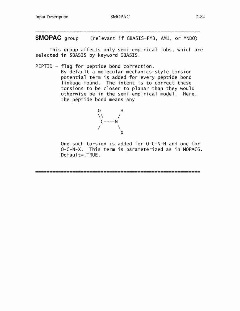
Input Description $MOPAC 2-84
==========================================================
$MOPAC group (relevant if GBASIS=PM3, AM1, or MNDO)
This group affects only semi-empirical jobs, which areselected in $BASIS by keyword GBASIS.
PEPTID = flag for peptide bond correction. By default a molecular mechanics-style torsion potential term is added for every peptide bond linkage found. The intent is to correct these torsions to be closer to planar than they would otherwise be in the semi-empirical model. Here, the peptide bond means any
O H \\ / C----N / \ X
One such torsion is added for O-C-N-H and one for O-C-N-X. This term is parameterized as in MOPAC6. Default=.TRUE.
==========================================================
Input Description $GUESS 2-85
==========================================================
$GUESS group (optional, relevant for all SCFTYP's)
This group controls the selection of initial molecularorbitals.
GUESS = Selects type of initial orbital guess. = HUCKEL Carry out an extended Huckel calculation using a Huzinaga MINI basis set, and project this onto the current basis. This is implemented for atoms up to Rn, and will work for any all electron or ECP basis set. (default for most runs) = HCORE Diagonalize the one electron Hamiltonian to obtain the initial guess orbitals. This method is applicable to any basis set, but does not work as well as the HUCKEL guess. = MOREAD Read in formatted vectors punched by an earlier run. This requires a $VEC deck, and you MUST pay attention to NORB below. = RDMINI Read in a $VEC deck from a converged calculation that used GBASIS=MINI and no polarization functions, and project these orbitals onto the current basis. Do not use this option if the current basis involve ECP basis sets. = MOSAVED (default for restarts) The initial orbitals are read from the DICTNRY file of the earlier run. = SKIP Bypass initial orbital selection. The initial orbitals and density matrix are assumed to be in the DICTNRY file. Mostly used for RUNTYP=HESSIAN when the hessian is being read in from the input.The next options are less general, being for FragmentMolecular Orbital runs, or Divide and Conquer runs: = FMO Read orbitals from the DICTNRY file, from previous FMO run with MODPRP=1. = HUCSUB Perform a Huckel guess in each subsystem of a Divide and Conquer run = DMREAD Read a density matrix from a formatted $DM

Input Description $GUESS 2-86
group, produced by a previous Divide and Conquer run, see NDCPRT in $DANDC.
All GUESS types except 'SKIP' permit reordering of theorbitals, carry out an orthonormalization of the orbitals,and generate the correct initial density matrix, for RHF,UHF, ROHF, and GVB, but note that correct computation ofthe GVB density requires also CICOEF in $SCF. The densitymatrix cannot be generated from the orbitals alone for MP2,CI, or MCSCF, so property evaluation for these should beRUNTYP=ENERGY rather than RUNTYP=PROP using GUESS=MOREAD.PRTMO = a flag to control printing of the initial guess. (default=.FALSE.)
PUNMO = a flag to control punching of the initial guess. (default=.FALSE.)
MIX = rotate the alpha and beta HOMO and LUMO orbitals so as to generate inequivalent alpha and beta orbital spaces. This pertains to UHF singlets only. This may require use of NOSYM=1 in $CONTRL depending on your situation. (default=.FALSE.)
NORB = The number of orbitals to be read in the $VEC group. This applies only to GUESS=MOREAD.
For -RHF-, -UHF-, -ROHF-, and -GVB-, NORB defaults to thenumber of occupied orbitals. NORB must be given for -CI-and -MCSCF-. For -UHF-, if NORB is not given, only theoccupied alpha and beta orbitals should be given, back toback. Otherwise, both alpha and beta orbitals mustconsist of NORB vectors.NORB may be larger than the number of occupied MOs, if youwish to read in the virtual orbitals. If NORB is lessthan the number of atomic orbitals, the remaining orbitalsare generated as the orthogonal complement to those read.
NORDER = Orbital reordering switch. = 0 No reordering (default) = 1 Reorder according to IORDER and JORDER.
IORDER = Reordering instructions. Input to this array gives the new molecular orbital order. For example, IORDER(3)=4,3 will interchange orbitals 3 and 4, while leaving the
Input Description $GUESS 2-87
other MOs in the original order. This parameter applies to all orbitals (alpha and beta) except for -UHF-, where it only affects the alpha MOs. (default is IORDER(i)=i )
JORDER = Reordering instructions. Same as IORDER, but for the beta MOs of -UHF-.
INSORB = the first INSORB orbitals specified in the $VEC group will be inserted into the Huckel guess, making the guess a hybrid of HUCKEL/MOREAD. This keyword is meaningful only when GUESS=HUCKEL, and it is useful mainly for QM/MM runs where some orbitals (buffer) are frozen and need to be transferred to the initial guess vector set, see $MOFRZ. (default=0)
* * * the next are 3 ways to clean up orbitals * * *
PURIFY = flag to symmetrize starting orbitals. This is the most soundly based of the possible procedures. However it may fail in complicated groups when the orbitals are very unsymmetric. (default=.FALSE.)
TOLZ = level below which MO coefficients will be set to zero. (default=1.0E-7)
TOLE = level at which MO coefficients will be equated. This is a relative level, coefficients are set equal if one agrees in magnitude to TOLE times the other. (default=5.0E-5)
SYMDEN = project the initial density in order to generate symmetric orbitals. This may be useful if the HUCKEL or HCORE guess types give orbitals of impure symmetry (?'s present). The procedure will generate a fairly high starting energy, and thus its use may not be a good idea for orbitals of the quality of MOREAD. (default=.FALSE.)
==========================================================
Input Description $VEC $DM $MOFRZ 2-88
==========================================================
$VEC group (optional, relevant for all SCFTYP's) (required if GUESS=MOREAD)
This group consists of formatted vectors, as writtenonto file PUNCH in a previous run. It is considered goodform to retain the titling comment cards punched beforethe $VEC card, as a reminder to yourself of the origin ofthe orbitals.
For Morokuma decompositions, the names of this groupare $VEC1, $VEC2, ... for each monomer, computed in theidentical orientation as the supermolecule. For transitionmoment or spin-orbit coupling runs, orbitals for statesone and possibly two are $VEC1 and $VEC2.
==========================================================
$DM group (relevant in Divide and Conquer runs)
This group consists of a formatted density matrix,read in exactly the format it was written. See GUESS=DM,and NDCPR in $DANDC.==========================================================
$MOFRZ group (optional, relevant for RHF, ROHF, GVB)
This group controls freezing the molecular orbitalsof your choice during the SCF procedure. If you choosethis option, select DIIS in $SCF since SOSCF will notconverge as well. GUESS=MOREAD is required in $GUESS.
FRZ = flag which triggers MO freezing. (default=.FALSE.)
IFRZ = an array of MOs in the input $VEC set which are to be frozen. There is no default for this.
==========================================================

Input Description $STATPT 2-89
==========================================================
$STATPT group (for RUNTYP=OPTIMIZE or SADPOINT)
This group controls the search for stationary points.Note that NZVAR in $CONTRL determines if the geometrysearch is conducted in Cartesian or internal coordinates.
METHOD = optimization algorithm selection. Pick from
NR Straight Newton-Raphson iterate. This will attempt to locate the nearest stationary point, which may be of any order. There is no steplength control. RUNTYP can be either OPTIMIZE or SADPOINT
RFO Rational Function Optimization. This is one of the augmented Hessian techniques where the shift parameter(s) is(are) chosen by a rational function approximation to the PES. For SADPOINT searches it involves two shift parameters. If the calculated stepsize is larger than DXMAX the step is simply scaled down to size.
QA Quadratic Approximation. This is another version of an augmented Hessian technique where the shift parameter is chosen such that the steplength is equal to DXMAX. It is completely equivalent to the TRIM method. (default)
SCHLEGEL The quasi-NR optimizer by Schlegel.
CONOPT, CONstrained OPTimization. An algorithm which can be used for locating TSs. The starting geometry MUST be a minimum! The algorithm tries to push the geometry uphill along a chosen Hessian mode (IFOLOW) by a series of optimizations on hyperspheres of increasingly larger radii. Note that there currently are no restart capabilitites for this method, not even manually.
Input Description $STATPT 2-90
OPTTOL = gradient convergence tolerance, in Hartree/Bohr. Convergence of a geometry search requires the largest component of the gradient to be less than OPTTOL, and the root mean square gradient less than 1/3 of OPTTOL. (default=0.0001)
NSTEP = maximum number of steps to take. Restart data is punched if NSTEP is exceeded. (default=20)
--- the next four control the step size ---
DXMAX = initial trust radius of the step, in Bohr. For METHOD=RFO, QA, or SCHLEGEL, steps will be scaled down to this value, if necessary. (default=0.3 for OPTIMIZE and 0.2 for SADPOINT) For METHOD=NR, DXMAX is inoperative. For METHOD=CONOPT, DXMAX is the step along the previous two points to increment the hypersphere radius between constrained optimizations. (default=0.1)
the next three apply only to METHOD=RFO or QA:
TRUPD = a flag to allow the trust radius to change as the geometry search proceeds. (default=.TRUE.)
TRMAX = maximum permissible value of the trust radius. (default=0.5 for OPTIMIZE and 0.3 for SADPOINT)
TRMIN = minimum permissible value of the trust radius. (default=0.05)
--- the next three control mode following ---
IFOLOW = Mode selection switch, for RUNTYP=SADPOINT. For METHOD=RFO or QA, the mode along which the energy is maximized, other modes are minimized. Usually refered to as "eigenvector following". For METHOD=SCHLEGEL, the mode whose eigenvalue is (or will be made) negative. All other curvatures will be made positive. For METHOD=CONOPT, the mode along which the geometry is initially perturbed from the minima. (default is 1)
Input Description $STATPT 2-91
In Cartesian coordinates, this variable doesn't count the six translation and rotation degrees. Note that the "modes" aren't from mass-weighting.
STPT = flag to indicate whether the initial geometry is considered a stationary point. If .true. the initial geometry will be perturbed by a step along the IFOLOW normal mode with stepsize STSTEP. (default=.false.) The positive direction is taken as the one where the largest component of the Hessian mode is positive. If there are more than one largest component (symmetry), the first is taken as positive. Note that STPT=.TRUE. has little meaning with HESS=GUESS as there will be many degenerate eigenvalues.
STSTEP = Stepsize for jumping off a stationary point. Using values of 0.05 or more may work better. (default=0.01)
IFREEZ = array of coordinates to freeze. These may be internal or Cartesian coordinates. For example, IFREEZ(1)=1,3 freezes the two bond lengths in the $ZMAT example, while optimizing the angle. If NZVAR=0, so that this value applies to the Cartesian coordinates instead, the input of IFREEZ(1)=4,7 means to freeze the x coordinates if the 2nd and 3rd atoms in the molecule.
See also IFZMAT and FVALUE in $ZMAT, and IFCART below, as IFREEZ does not apply to DLC internals.
In a numerical Hessian run, IFREEZ specifies Cartesian displacements to be skipped for a Partial Hessian Analysis. For more information: J.D.Head, Int.J.Quantum Chem. 65, 827, 1997 H.Li, J.H.Jensen Theoret. Chem. Acc. 107, 211-219(2002)
IFCART = array of Cartesian coordinates to freeze during a geometry optimization using delocalized internal coordinates.
Input Description $STATPT 2-92
--- The next two control the hessian matrix quality ---
HESS = selects the initial hessian matrix. = GUESS chooses an initial guess for the hessian. (default for RUNTYP=OPTIMIZE) = READ causes the hessian to be read from a $HESS group. (default for RUNTYP=SADPOINT) = RDAB reads only the ab initio part of the hessian, and approximates the effective fragment blocks. = RDALL reads the full hessian, then converts any fragment blocks to 6x6 T+R shape. (this option is seldom used). = CALC causes the hessian to be computed, see the $FORCE group.
IHREP = the number of steps before the hessian is recomputed. If given as 0, the hessian will be computed only at the initial geometry if you choose HESS=CALC, and never again. If nonzero, the hessian is recalculated every IHREP steps, with the update formula used on other steps. (default=0)
HSSEND = a flag to control automatic hessian evaluation at the end of a successful geometry search. (default=.FALSE.)
--- the next two control the amount of output --- Let 0 mean the initial geometry, L mean the last geometry, and all mean every geometry. Let INTR mean the internuclear distance matrix. Let HESS mean the approximation to the hessian. Note that a directly calculated hessian matrix will always be punched, NPUN refers only to the updated hessians used by the quasi-Newton step.
NPRT = 1 Print INTR at all, orbitals at all 0 Print INTR at all, orbitals at 0+L (default) -1 Print INTR at all, orbitals never -2 Print INTR at 0+L, orbitals never
NPUN = 3 Punch all orbitals and HESS at all 2 Punch all orbitals at all
Input Description $STATPT 2-93
1 same as 0, plus punch HESS at all 0 Punch all orbitals at 0+L, otherwise only occupied orbitals (default) -1 Punch occ orbitals at 0+L only -2 Never punch orbitals
---- the following parameters are quite specialized ----
PURIFY = a flag to help eliminate the rotational and translational degrees of freedom from the initial hessian (and possibly initial gradient). This is much like the variable of the same name in $FORCE, and will be relevant only if internal coordinates are in use. (default=.FALSE.)
PROJCT = a flag to eliminate translation and rotational degrees of freedom from Cartesian optimizations. The default is .TRUE. since this normally will reduce the number of steps, except that this variable is set false when POSITION=FIXED is used during EFP runs.
ITBMAT = number of micro-iterations used to compute the step in Cartesians which corresponds to the desired step in internals. The default is 5.
UPHESS = SKIP do not update Hessian (not recommended) BFGS default for OPTIMIZE using RFO or QA POWELL default for OPTIMIZE using NR or CONOPT POWELL default for SADPOINT MSP mixed Murtagh-Sargent/Powell update SCHLEGEL only choice for METHOD=SCHLEGEL
---- NNEG, RMIN, RMAX, RLIM apply only to SCHLEGEL ----
NNEG = The number of negative eigenvalues the force constant matrix should have. If necessary the smallest eigenvalues will be reversed. The default is 0 for RUNTYP=OPTIMIZE, and 1 for RUNTYP=SADPOINT.
RMIN = Minimum distance threshold. Points whose root mean square distance from the current point is less than RMIN are discarded. (default=0.0015)
Input Description $STATPT 2-94
RMAX = Maximum distance threshold. Points whose root mean square distance from the current point is greater than RMAX are discarded. (default=0.1)
RLIM = Linear dependence threshold. Vectors from the current point to the previous points must not be colinear. (default=0.07)==========================================================
* * * * * * * * * * * * * * * * * * * * * See the 'further information' section for some help with OPTIMIZE and SADPOINT runs * * * * * * * * * * * * * * * * * * * * *
Input Description $TRUDGE 2-95
==========================================================
$TRUDGE group (required for RUNTYP=TRUDGE)
This group defines the parameters for a non-gradientoptimization of exponents or the geometry. The TRUDGEpackage is a modified version of the same code from MichelDupuis' HONDO 7.0 system, origially written by H.F.King.Presently the program allows for the optimization of 10parameters.
Exponent optimization works only for uncontractedprimitives, without enforcing any constraints. Twonon-symmetry equivalent H atoms would have their pfunction exponents optimized separately, and so would twosymmetry equivalent atoms! A clear case of GIGO.
Geometry optimization works only in HINT internalcoordinates (see $CONTRL and $DATA groups). The totalenergy of all types of SCF wavefunctions can be optimized,although this would be extremely stupid as gradientmethods are far more efficient. The main utility is foropen shell MP2 or CI geometry optimizations, which maynot be done in any other way with GAMESS. If your runrequires NOSYM=1 in $CONTRL, you must be sure to use onlyC1 symmetry in the $DATA group.
OPTMIZ = a flag to select optimization of either geometry or exponents of primitive gaussian functions. = BASIS for basis set optimization. = GEOMETRY for geometry optimization (default). This means minima search only, there is no saddle point capability.
NPAR = number of parameters to be optimized.
IEX = defines the parameters to be optimized.
If OPTMIZ=BASIS, IEX declares the serial number of the Gaussian primitives for which the exponents will be optimized.
If OPTMIZ=GEOMETRY, IEX define the pointers to the HINT internal coordinates which will be optimized.
Input Description $TRUDGE 2-96
(Note that not all internal coordinates have to be optimized.) The pointers to the internal coordinates are defined as: (the number of atom on the input list)*10 + (the number of internal coordinate for that atom). For each atom, the HINT internal coordinates are numbered as 1, 2, and 3 for BOND, ALPHA, and BETA, respectively.
P = Defines the initial values of the parameters to be optimized. You can use this to reset values given in $DATA. If omitted, the $DATA values are used. If given here, geometric data must be in Angstroms and degrees.
A complete example is a TCSCF multireference 6-31Ggeometry optimization for methylene, $CONTRL SCFTYP=GVB CITYP=GUGA RUNTYP=TRUDGE COORD=HINT $END $BASIS GBASIS=N31 NGAUSS=6 $END $DATAMethylene TCSCF+CISD geometry optimizationCnv 2
C 6. LC 0.00 0.0 0.00 - O KH 1. PCC 1.00 53. 0.00 + O K I $END $SCF NCO=3 NPAIR=1 $END $TRUDGE OPTMIZ=GEOMETRY NPAR=2 IEX(1)=21,22 P(1)=1.08 $END $CIDRT GROUP=C2V SOCI=.TRUE. NFZC=1 NDOC=3 NVAL=1 NEXT=-1 $ENDusing GVB-PP(1), or TCSCF orbitals in the CI. The startingbond length is reset to 1.09, while the initial angle willbe 106 (twice 53). Result after 17 steps is R=1.1283056,half-angle=51.83377, with a CI energy of -38.9407538472
Note that you may optimize the geometry for an excitedCI state, just specify $GUGDIA NSTATE=5 $END $GUGDM IROOT=3 $ENDto find the equilibrium geometry of the third state (offive total states) of the symmetry implied by your $CIDRT.
==========================================================
Input Description $TRURST 2-97
==========================================================
$TRURST group (optional, relevant forRUNTYP=TRUDGE)
This group specifies restart parameters for TRUDGEruns and accuracy thresholds.
KSTART indicates the conjugate gradient direction in whichthe optimization will proceed. ( default = -1 ) -1 .... indicates that this is a non-restart run. 0 .... corresponds to a restart run.
FNOISE accuracy of function values.Variation smaller than FNOISE are not considered to besignificant (Def. 0.0005)
TOLF accuracy required of the function (Def. 0.001)
TOLR accuracy required of conjugate directions (Def. 0.05)
For geometry optimization, the values which givebetter results (closer to the ones obtained with gradientmethods) are: TOLF=0.0001, TOLR=0.001, FNOISE=0.00001
==========================================================
Input Description $FORCE 2-98
==========================================================
$FORCE group
(optional, relevant for RUNTYP=HESSIAN,OPTIMIZE,SADPOINT)
This group controls the computation of the hessianmatrix (the energy second derivative tensor, also knownas the force constant matrix), and an optional harmonicvibrational analysis. This can be a very time consumingcalculation. However, given the force constant matrix,the vibrational analysis for an isotopically substitutedmolecule is very cheap. Related input is HESS= in$STATPT, and the $MASS, $HESS, $GRAD, $DIPDR, $VIB groups.Calculation of the hessian automatically yields the dipolederivative tensor, giving IR frequencies. Ramanintensities are obtained by following with RUNTYP=RAMAN.
METHOD = chooses the computational method: = ANALYTIC is a fully analytic calculation. This is implemented for SCFTYP=RHF, ROHF, GVB (for NPAIR=0 or 1, only), and MCSCF (for CISTEP=ALDET or ORMAS, only). This is the default for these cases. = SEMINUM does numerical differentiation of analytically computed first derivatives. This is the default for UHF, MCSCF using other CISTEPs, DFT, all solvent, models, relativistic corrections, and most MP2 or CI runs. = FULLNUM numerically twice differentiates the energy, which can be used by all other cases. It requires many energies (a check run will tell how many) and so it is mainly useful for systems with only very few symmetry unique atoms.
The default for METHOD is to pick ANALYTIC over SEMINUM ifthat is programmed, and SEMINUM otherwise. FULLNUM willnever be chosen unless you specifically request it.
RDHESS = a flag to read the hessian from a $HESS group, rather than computing it. This variable pertains only to RUNTYP=HESSIAN. See also HESS= in the $STATPT group. (default is .FALSE.)
Input Description $FORCE 2-99
PURIFY = controls cleanup Given a $ZMAT, the hessian and dipole derivative tensor can be "purified" by transforming from Cartesians to internals and back to Cartesians. This effectively zeros the frequencies of the translation and rotation "modes", along with their IR intensities. The purified quantities are punched out. Purification does change the Hessian slightly, frequencies at a stationary point can change by a wave number or so. The change is bigger at non-stationary points. (default=.FALSE. if $ZMAT is given)
PRTIFC = prints the internal coordinate force constants. You MUST have defined a $ZMAT group to use this. (Default=.FALSE.)
--- the next four apply to numeric differentiation ----
NVIB = The number of displacements in each Cartesian direction for force field computation. This pertains only to SEMINUM, as FULLNUM always uses double difference formulae. = 1 Move one VIBSIZ unit in each positive Cartesian direction. This requires 3N+1 evaluations of the wavefunction, energy, and gradient, where N is the number of SYMMETRY UNIQUE atoms given in $DATA. (default) = 2 Move one VIBSIZ unit in the positive direction and one VIBSIZ unit in the negative direction. This requires 6N+1 evaluations of the wavefunction and gradient, and gives a small improvement in accuracy. In particular, the frequencies will change from NVIB=1 results by no more than 10-100 wavenumbers, and usually much less. However, the normal modes will be more nearly symmetry adapted, and the residual rotational and translational "frequencies" will be much closer to zero.
VIBSIZ = Displacement size (in Bohrs). This pertains to Both SEMINUM and FULLNUM. Default=0.01
Input Description $FORCE 2-100
Let 0 mean the Vib0 geometry, and D mean all the displaced geometries
NPRT = 1 Print orbitals at 0 and D = 0 Print orbitals at 0 only (default)
NPUN = 2 Punch all orbitals at 0 and D = 1 Punch all orbitals at 0 and occupied orbs at D = 0 Punch all orbitals at 0 only (default)
----- the rest control normal coordinate analysis ----
VIBANL = flag to activate vibrational analysis. (the default is .TRUE. for RUNTYP=HESSIAN, and otherwise is .FALSE.)
SCLFAC = scale factor for vibrational frequencies, used in calculating the zero point vibrational energy. Some workers correct for the usual overestimate in SCF frequencies by a factor 0.89. ZPE or other methods might employ other factors, see A.P.Scott, L.Radom J.Phys.Chem. 100, 16502-16513 (1996). The output always prints unscaled frequencies, so this value is used only during the thermochemical analysis. (Default is 1.0)
TEMP = an array of up to ten temperatures at which the thermochemistry should be printed out. The default is a single temperature, 298.15 K. To use absolute zero, input 0.001 degrees.
FREQ = an array of vibrational frequencies. If the frequencies are given here, the hessian matrix is not computed or read. You enter any imaginary frequencies as negative numbers, omit the zero frequencies corresponding to translation and rotation, and enter all true vibrational frequencies. Thermodynamic properties will be printed, nothing else is done by the run.
PRTSCN = flag to print contribution of each vibrational mode to the entropy. (Default is .FALSE.)
DECOMP = activates internal coordinate analysis.

Input Description $FORCE 2-101
Vibrational frequencies will be decomposed into "intrinsic frequencies", by the method of J.A.Boatz and M.S.Gordon, J.Phys.Chem., 93, 1819-1826(1989). If set .TRUE., the $ZMAT group may define more than 3N-6 (3N-5) coordinates. (default=.FALSE.)
PROJCT = controls the projection of the hessian matrix. The projection technique is described by W.H.Miller, N.C.Handy, J.E.Adams in J. Chem. Phys. 1980, 72, 99-112. At stationary points, the projection simply eliminates rotational and translational contaminants. At points with non-zero gradients, the projection also ensures that one of the vibrational modes will point along the gradient, so that there are a total of 7 zero frequencies. The other 3N-7 modes are constrained to be orthogonal to the gradient. Because the projection has such a large effect on the hessian, the hessian punched is the one BEFORE projection. For the same reason, the default is .FALSE. to skip the projection, which is mainly of interest in dynamical calculations.
==========================================================
There is a set of programs for the calculation of kineticor equilibrium isotope effects from the group of PiotrPaneth at the University of Lodz. The ISOEFF programaccepts data from GAMESS, and can be obtained [email protected].
Input Description $CPHF $MASS 2-102
==========================================================
$CPHF group (relevant for analytic RUNTYP=HESSIAN)
This group controls the solution of the responseequations, also known as coupled Hartree-Fock.
POLAR = a flag to request computation of the static polarizability, alpha. Because this property needs 3 additional response vectors, beyond those needed for the hessian, the default is to skip the property. (default = .FALSE.)
CPHF = MO forms response equations from transformed MO integrals. (default for ROHF/GVB/MCSCF) = AO forms response equations from AO integrals, which takes less memory, and is programmed only for RHF wavefunctions. (default if RHF) = AODDI forms response equations from AO integrals, using distributed memory (see MEMDDI). This does AO integrals about 2x more than AO, but spreads the CPHF memory requirement out across multiple nodes. Coded only for RHF.
SOLVER = linear equation solver choice. This is primarily a debugging option. For RHF analytic Hessians, choose from CONJG (default), DIIS, ONDISK, not all of which will work for all CPHF= choices. For imaginary frequency dependent polarizability responses (MAKEFP jobs), choose GMRES (default), biconjugate gradient stabilized BCGST, DODIIS, or an explicit solver GAUSS. Most response equations have only one solver programmed, and thus ignore this keyword.
NWORD = controls memory usage for this step. The default uses all available memory. (default=0)
==========================================================
$MASS group (relevant for RUNTYP=HESSIAN, IRC, or DRC)
This group permits isotopic substitution during thecomputation of mass weighted Cartesian coordinates. Ofcourse, the masses affect the frequencies and normal modes
Input Description $CPHF $MASS 2-103
of vibration.
AMASS = An array giving the atomic masses, in amu. The default is to use the mass of the most abundant isotope. Masses through element 104 are stored.
example - $MASS AMASS(3)=2.0140 $ENDwill make the third atom in the molecule a deuterium.
==========================================================

Input Description $HESS $GRAD 2-104
==========================================================
$HESS group (relevant for RUNTYP=HESSIAN if RDHESS=.TRUE.) (relevant for RUNTYP=IRC if FREQ,CMODE not given) (relevant for RUNTYP=OPTIMIZE,SADPOINT if HESS=READ)
Formatted force constant matrix (FCM), i.e. hessianmatrix. This data is punched out by a RUNTYP=HESSIAN job,in the correct format for subsequent runs. The first cardin the group must be a title card.
A $HESS group is always punched in Cartesians. Itwill be transformed into internal coordinate space if ageometry search uses internals. It will be mass weighted(according to $MASS) for IRC and frequency runs.
The initial FCM is updated during the course of ageometry optimization or saddle point search, and will bepunched if a run exhausts its time limit. This allowsrestarts where the job leaves off. You may want to readthis FCM back into the program for your restart, or youmay prefer to regenerate a new initial hessian. In anycase, this updated hessian is absolutely not suitable forfrequency prediction!
==========================================================
$GRAD group (relevant for RUNTYP=OPTIMIZE or SADPOINT) (relevant for RUNTYP=HESSIAN when RDHESS=.TRUE.)
Formatted gradient vector at the $DATA geometry. Thisdata is read in the same format it was punched out.
For RUNTYP=HESSIAN, this information is used todetermine if you are at a stationary point, and possiblyfor projection. If omitted, the program pretends thegradient is zero, and otherwise proceeds normally.
For geometry searches, this information (if known) canbe read into the program so that the first step can betaken instantly.
==========================================================

Input Description $DIPDR $VIB $VIB2 2-105
==========================================================
$DIPDR group (relevant for RUNTYP=HESSIAN if RDHESS=.T.)
Formatted dipole derivative tensor, punched in a previousRUNTYP=HESSIAN job. If this group is omitted, then avibrational analysis will be unable to predict the IRintensities, but the run can otherwise proceed.
==========================================================
$VIB group (relevant for RUNTYP=HESSIAN, METHOD=SEMINUM)
Formatted restart data, consisting of energies,gradients, and dipole moments. This data is read in thesame format by which is was written to the RESTART file.Just add a " $END" card, and place this group into theinput file to effect a restart. If the final gradient waswritten as zero, delete the entire last data set (energy,gradient, and dipole).
This group can also be used to turn a less accurate singledifferencing run into a more accurate double differencingrun (NVIB in $HESS).
The mere presence of this group triggers the restart.==========================================================
$VIB2 group (relevant for hessians, METHOD=FULLNUM) (relevant for gradients, with NUMGRD=.TRUE.)
Formatted restart information, consisting of energy values,as written to the RESTART file. Just add a " $END" line atthe bottom, and place this group into the input file toeffect a restart. This group has the same name ($VIB2),but different contents, depending on whether you arerestarting a numerical gradient or a fully numericalhessian job.
The mere presence of this group triggers the restart.===========================================================
Input Description $VSCF 2-106
==========================================================
$VSCF group (optional, relevant to RUNTYP=VSCF)
This group governs the computation of vibrationalfrequencies including anharmonic effects. Besides thekeywords shown below, the input file must contain a $HESSgroup (and perhaps a $DIPDR group), to start withpreviously obtained harmonic vibrational information. TheVSCF method requires only energies, so any energy type inGAMESS may be used, perhaps with fully numerical harmonicvibrational information. Energies are sampled along thedirections of the harmonic normal modes, and usually alongpairs of harmonic normal modes, after which the nuclearvibrational wavefunctions are obtained. The dipole on thegrid points may be used to give improved IR intensities.
The most accurate calculation computes the potentialsurface directly, on all grid points, but this involvesmany energy evaluations. An attractive alternative is theQuartic Force Field approximation of Yagi et al., whichcomputes a fit to the derivatives up to fourth order bycomputing a specialized set of points, after which this fitis used to generate the full grid of points for the solver.
Since there are a great many independent energyevaluations, no matter which type of surface is computed,the VSCF method allows for computations in subgroups (muchlike the FMO method). Thus the $GDDI group will be readand acted upon, if found.
Vibrational wavefunctions are obtained at an SCF-likelevel, termed VSCF, using product nuclear wavefunctions,along with an MP2-like correction to the vibrationalenergy, which is termed correlation corrected (cc-VSCF).In addition, vibrational energy levels based on secondorder degenerate pertubation theory (see VDPT) or a CIanalog (see VCI) may be obtained.
Most VSCF applications have been carried out with anelectronic structure level of MP2 with triple zeta basissets. This is thought to give accuracy to 50 wavenumbersfor the larger fundamentals. Use of internal coordinatesis known to give improved accuracy for lower frequencies,particularly in weakly bound clusters.
Input Description $VSCF 2-107
Restarts involve the $VIBSCF group (which has differentformats for each PETYP), and the READV keyword. Restartsare safest on the same machine, where normal mode phasesare reproducible.
References for the VSCF method, the QFF approximation,and the solvers are given in Chapter 4 of this manual,along with a number of sample applications.
* * * * *
The first input variables control the generation of thepotential surface on which the nuclear vibrations occur:
PETYP = DIRECT computes the full potential energy surface, according to NCOUP/NGRID. The total number of energy/dipole calculations for NCOUP=2 will be M*NGRID + (M*(M-1)/2)*NGRID*NGRID, where M is the number of normal modes. This is the default. = QFF the Quartic Force Field approximation to the potential surface is obtained. This is usually only slightly less accurate, but has a greatly reduced computational burden, namely 6*M + 12*M*(M-1)/2 energy/dipoles.
INTCRD = flag setting the coordinate system used for the grids. Any internal coordinates to be used must be defined in $ZMAT, using only 3N-6 simple coordinates (no DLC or natural internals), and of course you must give NZVAR in $CONTRL as well. The default is to use Cartesians (default .FALSE.)
INTTYP = 0 default if INTCRD=.FALSE. (ignore this keyword) = 1 implies that the $ZMAT contains only stretches, bends, and torsions. It also selects an approximate transformation between Cartesian and internal coords. = 2 the other $ZMAT coordinates may be used, and the coordinate transformation will be iterated to convergence. (default if INTCRD=.TRUE.)
NCOUP = the order of mode couplings included.

Input Description $VSCF 2-108
= 1 computes 1-D grids along each harmonic mode = 2 adds additionally, 2-D grids along each pair of normal modes. (default=2) = 3 adds additionally, 3-D grids for mode triples, for PETYP=DIRECT only.
NGRID = number of grid points to be used in solving for the anharmonic vibrational levels. In the case of PETYP=DIRECT, each of these grid points must be explicitly computed. For PETYP=QFF these grid points are obtained from a fitted quartic force field. Reasonable values are 8 or 16 for DIRECT, with 16 considered significantly more accurate. For PETYP=QFF, the generation of the solver grid is very fast, so use 16 always. (default=16)
AMP = step size for PETYP=DIRECT displacements. The maximum distance along each mode is a function of its frequency, amplitude(i)=sqrt(2*(AMP+1/2)/freq(i)) so that AMP resembles a vibrational quantum number. The default goes far enough past the classical turning points of the fundamentals to capture the relevant part of the surface. (default = 7.0)
STPSZ = step size for PETYP=QFF displacements. The step along each mode depends on the harmonic frequency, as well as this parameter, whose default is usually satisfactory (default=0.5)
In case the user wants to control each normal mode with aseparate parameter, arrays of values may be given, usingthe keywords AMPX(1)=xx,yy,... or STPSZX(1)=xx,yy,zz...
IMODE = array of modes for which anharmonic effects will be computed. IMODE(1)=10,19 computes anharmonic energies and wavefunctions for modes 10 and 19, only. In the current implementation, pairs of modes cannot be coupled, so NCOUP is forced to 1 if this option is specified. This approximation is intended for larger molecules, where the whole VSCF calculation is prohibitive.
* * * * *
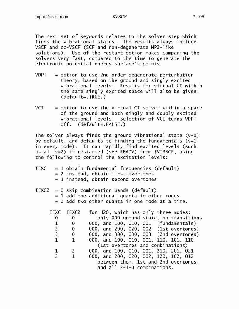
Input Description $VSCF 2-109
The next set of keywords relates to the solver step whichfinds the vibrational states. The results always includeVSCF and cc-VSCF (SCF and non-degenerate MP2-likesolutions). Use of the restart option makes comparing thesolvers very fast, compared to the time to generate theelectronic potential energy surface's points.
VDPT = option to use 2nd order degenerate perturbation theory, based on the ground and singly excited vibrational levels. Results for virtual CI within the same singly excited space will also be given. (default=.TRUE.)
VCI = option to use the virtual CI solver within a space of the ground and both singly and doubly excited vibrational levels. Selection of VCI turns VDPT off. (default=.FALSE.)
The solver always finds the ground vibrational state (v=0)by default, and defaults to finding the fundamentals (v=1in every mode). It can rapidly find excited levels (suchas all v=2) if restarted (see READV) from $VIBSCF, usingthe following to control the excitation levels:
IEXC = 1 obtain fundamental frequencies (default) = 2 instead, obtain first overtones = 3 instead, obtain second overtones
IEXC2 = 0 skip combination bands (default) = 1 add one additional quanta in other modes = 2 add two other quanta in one mode at a time.
IEXC IEXC2 for H2O, which has only three modes: 0 0 only 000 ground state, no transitions 1 0 000, and 100, 010, 001 (fundamentals) 2 0 000, and 200, 020, 002 (1st overtones) 3 0 000, and 300, 030, 003 (2nd overtones) 1 1 000, and 100, 010, 001, 110, 101, 110 (1st overtones and combinations) 1 2 000, and 100, 010, 001, 210, 201, 021 2 1 000, and 200, 020, 002, 120, 102, 012 between them, 1st and 2nd overtones, and all 2-1-0 combinations.

Input Description $VSCF 2-110
ICAS1, ICAS2 = starting and ending vibrations whose quanta are included. The default is all modes, ICAS1=1 and ICAS2=3N-6 (or 3N-5).
SFACT = a numerical cutoff for small contributions in the solver. The default is 1d-4: 5d-3 or 1d-3 may affect accuracy of results, 1d-4 is safer, and 1d-5 might not converge.
VCFCT = scaling factor for pair-coupling potential. Sometimes when pair-coupling potential values are larger than the corresponding single mode values, they must be scaled down. It is seldom necessary to select a scaling other than unity. (Default=1.0)
* * * * *
The next two relate to simplified intensity computation.These simplifications are aimed at speeding up MP2 runs, ifone does not care so much about intensities, and would liketo eliminate the considerable extra time to compute MP2-level dipoles. DMDR must not be used if overtones arebeing computed.
DMDR = if true, indicates that the harmonic dipole derivative tensor $DIPDR will be read and used, rather than computing dipoles. (default=.FALSE.)
MPDIP = for MP2 electronic structure, a value of .FALSE. uses SCF level dipoles in order to save the time needed to obtain the MP2 density at every grid point. It is more accurate to use the DMDR flag instead of this option, if an MP2 level $DIPDR is available. (default=.TRUE.)
* * * * *
PROJCT = controls the projection of the hessian matrix (same meaning as in $FORCE). Default is .TRUE. which removes small mixings between rotations or translations and the harmonic modes.
READV = flag to indicate restart data $VIBSCF should be read in to resume an interrupted calculation, or
Input Description $VSCF 2-111
to obtain overtones in follow-on runs. (default is .FALSE.)
==========================================================
$VIBSCF group (optional, relevant to RUNTYP=VSCF)This is restart data, as written to the disk file RESTARTin a complete or partially completed previous run. Appenda " $END", and also select READV=.TRUE. to read the data.
$VIBSCF's contents are different for PETYP=DIRECT or QFF.
The format of this group changed in December 2006, so thatold groups can no longer be used.
==========================================================
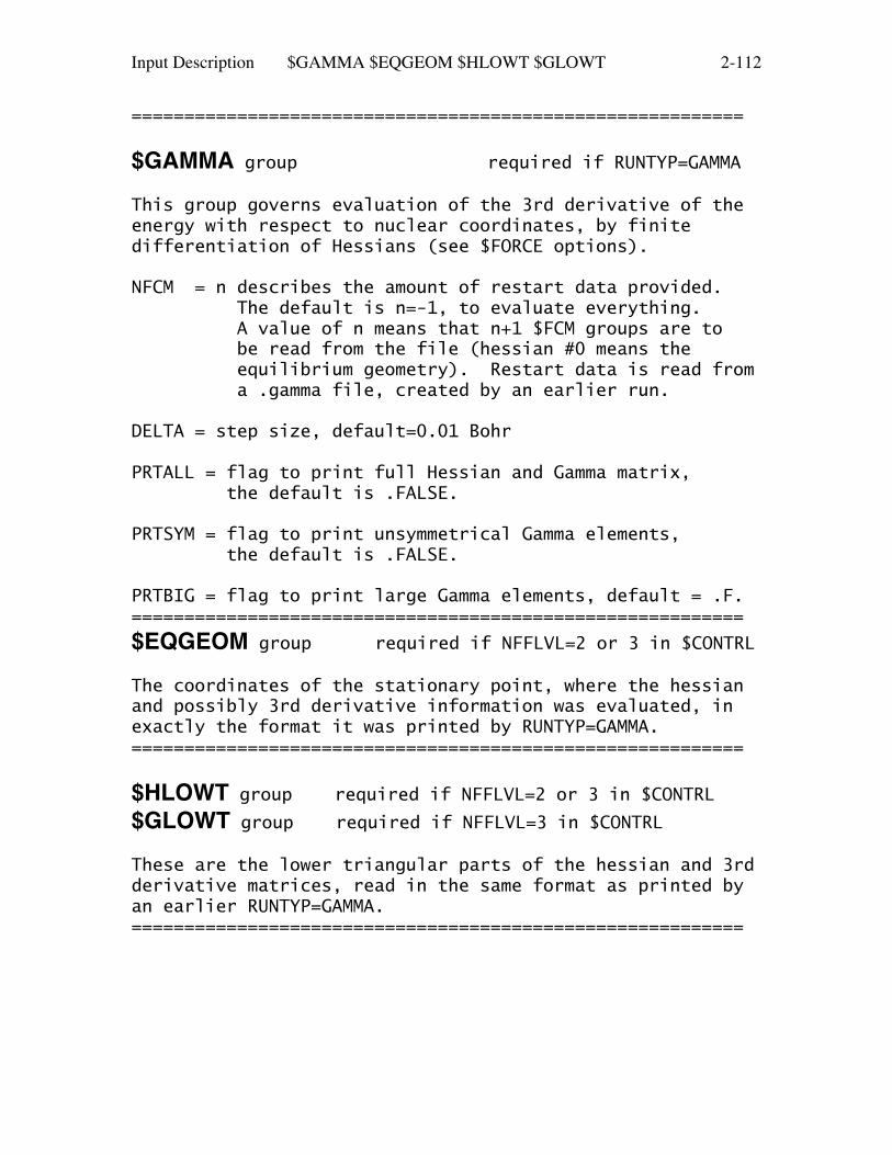
Input Description $GAMMA $EQGEOM $HLOWT $GLOWT 2-112
==========================================================
$GAMMA group required if RUNTYP=GAMMA
This group governs evaluation of the 3rd derivative of theenergy with respect to nuclear coordinates, by finitedifferentiation of Hessians (see $FORCE options).
NFCM = n describes the amount of restart data provided. The default is n=-1, to evaluate everything. A value of n means that n+1 $FCM groups are to be read from the file (hessian #0 means the equilibrium geometry). Restart data is read from a .gamma file, created by an earlier run.
DELTA = step size, default=0.01 Bohr
PRTALL = flag to print full Hessian and Gamma matrix, the default is .FALSE.
PRTSYM = flag to print unsymmetrical Gamma elements, the default is .FALSE.
PRTBIG = flag to print large Gamma elements, default = .F.==========================================================
$EQGEOM group required if NFFLVL=2 or 3 in $CONTRL
The coordinates of the stationary point, where the hessianand possibly 3rd derivative information was evaluated, inexactly the format it was printed by RUNTYP=GAMMA.==========================================================
$HLOWT group required if NFFLVL=2 or 3 in $CONTRL$GLOWT group required if NFFLVL=3 in $CONTRL
These are the lower triangular parts of the hessian and 3rdderivative matrices, read in the same format as printed byan earlier RUNTYP=GAMMA.==========================================================
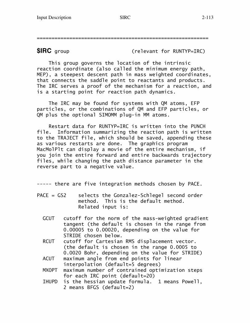
Input Description $IRC 2-113
==========================================================
$IRC group (relevant for RUNTYP=IRC)
This group governs the location of the intrinsicreaction coordinate (also called the minimum energy path,MEP), a steepest descent path in mass weighted coordinates,that connects the saddle point to reactants and products.The IRC serves a proof of the mechanism for a reaction, andis a starting point for reaction path dynamics.
The IRC may be found for systems with QM atoms, EFPparticles, or the combinations of QM and EFP particles, orQM plus the optional SIMOMM plug-in MM atoms.
Restart data for RUNTYP=IRC is written into the PUNCHfile. Information summarizing the reaction path is writtento the TRAJECT file, which should be saved, appending theseas various restarts are done. The graphics programMacMolPlt can display a movie of the entire mechanism, ifyou join the entire forward and entire backwards trajectoryfiles, while changing the path distance parameter in thereverse part to a negative value.
----- there are five integration methods chosen by PACE.
PACE = GS2 selects the Gonzalez-Schlegel second order method. This is the default method. Related input is:
GCUT cutoff for the norm of the mass-weighted gradient tangent (the default is chosen in the range from 0.00005 to 0.00020, depending on the value for STRIDE chosen below. RCUT cutoff for Cartesian RMS displacement vector. (the default is chosen in the range 0.0005 to 0.0020 Bohr, depending on the value for STRIDE) ACUT maximum angle from end points for linear interpolation (default=5 degrees) MXOPT maximum number of contrained optimization steps for each IRC point (default=20) IHUPD is the hessian update formula. 1 means Powell, 2 means BFGS (default=2)
Input Description $IRC 2-114
GA is a gradient from the previous IRC point, and is used when restarting. OPTTOL is a gradient cutoff used to determine if the IRC is approaching a minimum. It has the same meaning as the variable in $STATPT. (default=0.0001)
PACE = LINEAR selects linear gradient following (Euler's method). Related input is:
STABLZ switches on Ishida/Morokuma/Komornicki reaction path stabilization. The default is .TRUE. DELTA initial step size along the unit bisector, if STABLZ is on. Default=0.025 Bohr. ELBOW is the collinearity threshold above which the stabilization is skipped. If the mass weighted gradients at QB and QC are almost collinear, the reaction path is deemed to be curving very little, and stabilization isn't needed. The default is 175.0 degrees. To always perform stabilization, input 180.0. READQB,EB,GBNORM,GB are energy and gradient data already known at the current IRC point. If it happens that a run with STABLZ on decides to skip stabilization because of ELBOW, this data will be punched to speed the restart.
PACE = QUAD selects quadratic gradient following. Related input is:
SAB distance to previous point on the IRC. GA gradient vector at that historical point.
PACE = AMPC4 selects the fourth order Adams-Moulton variable step predictor-corrector. Related input is:
GA0,GA1,GA2 which are gradients at previous points.
PACE = RK4 selects the 4th order Runge-Kutta variable step method. There is no related input.
Input Description $IRC 2-115
----- The next two are used by all PACE choices -----
STRIDE = Determines how far apart points on the reaction path will be. STRIDE is used to calculate the step taken, according to the PACE you choose. The default is good for the GS2 method, which is very robust. Other methods should request much smaller step sizes, such as 0.10 or even 0.05. (default = 0.30 sqrt(amu)-Bohr)NPOINT = The number of IRC points to be located in this run. The default is to find only the next point. (default = 1)
----- The next two let you choose your output volume -----
Let F mean the first IRC point found in this run, and L mean the final IRC point of this run. Let INTR mean the internuclear distance matrix.
NPRT = 1 Print INTR at all, orbitals at all IRC points 0 Print INTR at all, orbitals at F+L (default) -1 Print INTR at all, orbitals never -2 Print INTR at F+L, orbitals never
NPUN = 1 Punch all orbitals at all IRC points 0 Punch all orbitals at F+L, only occupied orbitals at IRC points between (default) -1 Punch all orbitals at F+L only -2 Never punch orbitals
----- The next two tally the reaction path results. The defaults are appropriate for starting from a saddle point, restart values are automatically punched out.
NEXTPT = The number of the next point to be computed.STOTAL = Total distance along the reaction path to next IRC point, in mass weighted Cartesian space.
----- The following controls jumping off the saddle point.
Input Description $IRC 2-116
If you give a $HESS group, FREQ and CMODE will be generated automatically.
SADDLE = A logical variable telling if the coordinates given in the $DATA deck are at a saddle point (.TRUE.) or some other point lying on the IRC (.FALSE.). If SADDLE is true, either a $HESS group or else FREQ and CMODE must be given. (default = .FALSE.) Related input is:
TSENGY = A logical variable controlling whether the energy and wavefunction are evaluated at the transition state coordinates given in $DATA. Since you already know the energy from the transition state search and force field runs, the default is .F.FORWRD = A logical variable controlling the direction to proceed away from a saddle point. The forward direction is defined as the direction in which the largest magnitude component of the imaginary normal mode is positive. (default =.TRUE.)EVIB = Desired decrease in energy when following the imaginary normal mode away from a saddle point. (default=0.0005 Hartree)FREQ = The magnitude of the imaginary frequency, given in cm**-1.CMODE = An array of the components of the normal mode whose frequency is imaginary, in Cartesian coordinates. Be careful with the signs!
You must give FREQ and CMODE if you don't give a $HESS group, when SADDLE=.TRUE. The option of giving these two variables instead of a $HESS does not apply to the GS2 method, which must have a hessian input, even for restarts. Note also that EVIB is ignored by GS2 runs.
* * * * * * * * * * * * * * * * * * For hints about IRC tracking, see the 'further information' section. * * * * * * * * * * * * * * * * * *
==========================================================
Input Description $DRC 2-117
==========================================================
$DRC group (relevant for RUNTYP=DRC)
This group governs "direct dynamics", following thedynamical reaction coordinate, which is a classicaltrajectory based on quantum chemistry potential energysurfaces. These may be either ab initio or semi-empirical,and are computed "on the fly" as the trajectory proceeds.
Because the vibrational period of a normal mode withfrequency 500 wavenumbers is 67 fs, a DRC needs to run formany steps in order to sample a representative portion ofphase space. Restart data can be found in the job's OUTPUTfile, with important results summarized to the TRAJECTfile. Almost all DRCs break molecular symmetry, so buildyour molecule with C1 symmetry in $DATA, or specify NOSYM=1in $CONTRL. RUNTYP=DRC may not be used with EFP particles.
NSTEP = The number of DRC points to be calculated, not including the initial point. (default = 1000)
DELTAT = is the time step. (default = 0.1 fs)
TOTIME = total duration of the DRC computed in a previous job, in fs. The default is the correct value when initiating a DRC. (default=0.0 fs)
* * *
In general, a DRC can be initiated anywhere, so $DATA might contain coordinates of the equilibrium geometry, or a nearby transition state, or something else. You must also supply an initial kinetic energy, and the direction of the initial velocity, for which there are a number of options:
EKIN = The initial kinetic energy (default = 0.0kcal/mol) See also ENM, NVEL, and VIBLVL regarding alternate ways to specify the initial value.
VEL = an array of velocity components, in Bohr/fs. When NVEL is false, this is simply the direction
Input Description $DRC 2-118
of the velocity vector. Its magnitude will be automatically adjusted to match the desiredinitial kinetic energy, and it will be projected so that the translation of the center of mass is removed. Give in the order vx1, vy1, vz1, vx2, vy2, ...
NVEL = a flag to compute the initial kinetic energy from the input VEL using the sum of mass*VEL*VEL/2. This flag is usually selected only for restarts. (default=.FALSE.)
The next three allow the kinetic energy to be partitioned over all normal modes. The coordinates in $DATA are likely to be from a stationary point! You must also supply a $HESS group, which is the nuclear force constant matrix at the starting geometry.
VIBLVL = a flag to turn this option on (default=.FALSE.)
VIBENG = an array of energies (in units of multiples of the hv of each mode) to be imparted along each normal mode. The default is to assign the zero point energy only, VIBENG(1)=0.5, 0.5, ..., 0.5 when HESS=MIN, and 0.0, 0.5, ..., 0.5 if HESS=TS. If given as a negative number, the initial direction of the velocity vector is along the reverse direction of the mode. "Reverse" means the phase of the normal mode is chosen such that the largest magnitude component is a negative value. An example might be VIBENG(4)=2.5 to add two quanta to mode 4, along with zero point energy in all modes.
RCENG = reaction coordinate energy, in kcal/mol. This is the initial kinetic energy given to the imaginary frequency normal mode when HESS=TS. If this is given as a negative value, the direction of the velocity vector will be the "reverse direction", meaning the phase of the normal mode will be chosen so its largest component is negative.
* * *
Input Description $DRC 2-119
The next two pertain to initiating the DRC along a single normal mode of vibration. No kinetic energy is assigned to the other modes. You must also supply a $HESS group at the initial geometry.
NNM = The number of the normal mode to which the initial kinetic energy is given. The absolute value of NNM must be in the range 1, 2, ..., 3N-6. If NNM is a positive/negative value, the initial velocity will lie in the forward/reverse direction of the mode. "Forward" means the largest normal mode component is a positive value. (default=0)
ENM = the initial kinetic energy given to mode NNM, in units of vibrational quanta hv, so the amount depends on mode NNM's vibrational frequency, v. If you prefer to impart an arbitrary initial kinetic energy to mode NNM, specify EKIN instead. (default = 0.0 quanta)
To summarize, there are 5 ways to initiate a trajectory:
1. VEL vector with NVEL=.TRUE. This is difficult to specify at your initial point, and so this option is mainly used when restarting your trajectory. The restart information is always in this format. 2. VEL vector and EKIN with NVEL=.FALSE. This will give a desired amount of kinetic energy in the direction of the velocity vector. 3. VIBLVL and VIBENG and possibly RCENG, to give some initial kinetic energy to all normal modes. 4. NNM and ENM to give quanta to a single normal mode. 5. NNM and EKIN to give arbitrary kinetic energy to a single normal mode.
* * *
The most common use of the next two is to analyze a trajectory with respect to the normal modes of a minimum energy geometry it travels around.
NMANAL = a flag to select mapping of the mass-weighted Cartesian DRC coordinates and velocity (conjugate momentum) in terms of normal modes at a nearby
Input Description $DRC 2-120
reference stationary point (which can be either a minimum or transition state). This reference geometry could in fact be the same as the initial point of the DRC, but does not need to be. If you choose this option, you must supply C0, HESS2, and a $HESS2 group corresponding to the reference stationary point. (default=.FALSE.)
C0 = an array of the coordinates of the stationary reference point (the coordinates in $DATA might well be some other coordinates). Give in the order x1,y1,z1,x2,y2,... in Angstroms.
* * *
The next options apply to input choices which may read a $HESS at the initial DRC point, namely NNM or VIBLVL, or to those that read a $HESS2 at some reference geometry (NMANAL).
HESS = MIN indicates the hessian supplied for the initial geometry corresponds to a minimum (default). = TS indicates the hessian is for a saddle point.HESS2 = MIN (default) or TS, the same meaning, for the reference geometry.
These are used to decide if modes 1-6 (minimum) or modes 2-7 (TS) are to be excluded from the hessian as the translational and rotational contaminants. If the initial and reference geometries are the same, these two hessians will be duplicates of each other.
The next variables can cause termination of a run, ifmolecular fragments get too far apart or close together.
NFRGPR = Number of atom pairs whose distance will be checked. (default is 0)
IFRGPR = Array of the atom pairs. 2 times NFRGPR values.
FRGCUT = Array for a boundary distance (in Bohr) for atom pairs to end DRC calculations. The run will stop if any distance exceeds the tolerance, or if a value is given as a negative number, if the

Input Description $DRC 2-121
distance becomes shorter than the absolute value. In case the trajectory starts outside the bounds specified, they do not apply until after the trajectory reaches a point where the criteria are satisfied, and then goes outside again. Give NFRGPR values.
* * *
The final variables control the volume of output. Let F mean the first DRC point found in this run, and L mean the last DRC point of this run.
NPRTSM = summarize the DRC results every NPRTSM steps, to the TRAJECT file. (default = 1)
NPRT = 1 Print orbitals at all DRC points 0 Print orbitals at F+L (default) -1 Never print orbitals
NPUN = 2 Punch all orbitals at all DRC points 1 Punch all orbitals at F+L, and occupied orbitals at DRC points between 0 Punch all orbitals at F+L only (default) -1 Never punch orbitals
==========================================================
Input Description $MEX 2-122
===========================================================
$MEX group (relevant if RUNTYP=MEX)
This group governs a search for the lowest energy on the3N-7 dimensional "seam" of intersection of two differentelectronic potential energy surfaces. Such Minimum EnergyCrossing Points are important for processes such as spin-orbit coupling that involve transfer from one surface toanother, and thus are analogous to transition states on asingle surface. The present program requires that the twosurfaces differ in spin quantum number, or space symmetry,or both. Analytic gradients are used in the search.
SCF1, SCF2 = define the molecular wavefunction types, possibly in conjunction with the usual MPLEVL and DFTTYP keywords.
MULT1, MULT2 = give the spin multiplicity of the states.
Permissible combinations of wavefunctions are RHF with ROHF/UHF ROHF with ROHF UHF with UHF as well as their MP2 and DFT counterparts, and GVB with ROHF/UHF MCSCF with MCSCF (CISTEP=ALDET or GUGA only)
NSTEP = maximum number of search steps (default=50)
STPSZ = Step size during the search (default = 0.1D+00)
NRDMOS = Initial orbitals can be read in = 0 No initial orbitals (default) = 1 Read in orbitals for first state (in $VEC1) = 2 Read in orbitals for second state (in $VEC2) = 3 Read in orbitals for both ($VEC1 and $VEC2)
NMOS1 = Number of orbitals for first state's $VEC1.
NMOS2 = Number of orbitals for second state's $VEC2.
NPRT = Printing orbitals
Input Description $MEX 2-123
= 0 No orbital printed out except at the first geometry (default) = 1 Orbitals are printed each geometry. If MCSCF is used, CI expansions are also printed.
Finer control of the convergence criterion:
TDE = energy difference between two states (default = 1.0D-05)
TDXMAX = maximum displacement of coordinates (default = 2.0D-03)
TDXRMS = root mean square displacement (default = 1.5D-03)
TGMAX = maximum of effective gradient between the two states (default = 5.0D-04)
TGRMS = root mean square effective gradient tolerance (default = 3.0D-04)
===========================================================
Usage notes:
1. Normally $CONTRL will not give SCFTYP or MULT keywords.SCF1 and SCF2 can be given in any order. The combinationspermitted ensure roughly equal sophistication in thetreatment of electron correlation.2. After reading $MEX, SCFTYP and MULT will be set to themore complex of the two choices, which is considered to beRHF < ROHF < UHF < GVB < MCSCF. This permits the $SCFinput defining a GVB wavefunction to be read and tested forcorrectness, in a GVB+ROHF run. Since only one SCFTYP isstored while reading the input, you might need to providesome keywords that are normally set by default for theother (such as ensuring DIIS is selected in $SCF if eitherof the states is UHF).3. It is safest by far to prepare and read $VEC1 and $VEC2groups so that you know what electronic states you startwith. It is a good idea to regenerate both states at theend of the MEX search, to be sure that they remain as youbegan.

Input Description $MEX 2-124
4. It is your responsibility to make sure that the stateshave a different space symmetry, or a different spinsymmetry (or both). That is why note 3 is so important.5. $GRAD1 and/or $GRAD2 groups containing gradients may begiven to speed up the first geometry of the MEX search.6. The search is even trickier than a saddle point search,for it involves the peaks and valleys of BOTH surfacesbeing generated. Starting geometries may be guessed aslying between the minima of the two surfaces, but thelowest energy on the crossing seam may turn out to besomewhere else. Be prepared to restart!7. The procedure is a Newton-Raphson search, conducted inCartesian coordinates, with a Lagrange multiplier imposingthe constraint of equal energy upon the two states. Thehessian matrices in the search are guessed at, andsubjected to BFGS updates. Internal coordinates will beprinted (for monitoring purposes) if you define $ZMAT, butthe stepper operates in Cartesian coordinates only. Nogeometry constraints can be applied, apart from the pointgroup in $DATA.
A good paper to read about this kind of search isA.Farazdel, M.Dupuis J.Comput.Chem. 12, 276-282(1991)
Input Description $MD 2-125
===========================================================
$MD group (relevant if RUNTYP=MD)
This group controls the molecular dynamics trajectory for acollection of quantum mechanical atoms and/or EffectiveFragment Potential particles.
A typical MD simulation starts with an equilibration phase,running long enough to produce a randomized structure andvelocity distribution. Typically equilibration is donewith an NVT ensemble, allowing the system to equilibrate toa desired temperature. A production run restarts with thepositions and the velocity and quaternion data from theequilibration run, might use either a NVE or NVT ensemble,and collects radial distribution functions and otherproperties.
Only a few properties are computed from the MD trajectory,apart from correct radial distribution functions. Inparticular, the pressures, diffusion constants, and heatsof vaporization that appear on the printout (presently onlyfor pure EFP runs) are from a preliminary code, which hasnot yet been verified.
If the system contains only EFP particles, it may be placedin a periodic box, according to the minimum imageconvention. The optional periodic boundary conditions,along with cut-offs, are given in the $EFRAG group. Seealso the $EWALD input group for long-range electrostatictreatment if PBC is used.
The first keywords relate to the steps:
MDINT = MD integrator selection. = FROG (leapfrog). This is less accurate, and lacks the special ensemble stepper option NVTNH. = VVERLET (velocity Verlet) - default.
DT = MD time step size, in seconds, default=1.0d-15, which is a femtosecond.
NVTNH selects a integrator step appropriate to the desired ensemble. This is only implemented for

Input Description $MD 2-126
velocity Verlet. = 0 means use NVE Verlet stepping = 1 means use NVT Verlet stepping = 2 means use Nose/Hoover chain NVT Verlet stepping The default is 2 if either NVT option RSTEMP or RSRAND is chosen, but is 0 otherwise.
NSTEPS = number of MD time steps to be found in this run, default=10000.
NTOTAL = number of time steps previously found on the MD trajectory, which is being restarted (see READ=.TRUE.). The default=0, meaning that this trajectory is a new one, or is perhaps the start of a production phase of the MD.
* * *
BATHT = bath temperature, in Kelvin (default=300.0) This value is used during NVT runs, or if the MD is initialized to a Maxwell-Boltzmann velocity distribution.
* * *
Two options exist to create NVT runs, to bring the system to a desired bath temperature. If neither is chosen, the ensemble is NVE:
RSTEMP = flag to rescale the temperature. default=.FALSE.
DTEMP = temperature range for the RSTEMP option. The velocities are rescaled to the bath temperature if T < (BATHT-DTEMP) or T > (BATHT+DTEMP). The default is DTEMP=100.0 degrees.
RSRAND = flag to reset to Maxwell-Boltzmann distribution, using random numbers (same algorithm as MBT and MBR) to choose individual velocity magnitudes and directions. default=.FALSE.
NRAND = number of steps for the RSRAND option. Reassign velocities (translational and rotational) every NRAND time steps. Default=1000.

Input Description $MD 2-127
NVTOFF = step number at which to turn off either NVT thermostat, and switch to NVE. At this point, the NVTNH parameter will be reset to 0, and the PROD flag will be turned on, so that the production run will start (gathering and printing the RDF information to .log file). This keyword is also useful in NVE runs to postpone the accumulation of production information. The default means no switch to NVE (default=0).
JEVERY = report simulation quantities (write info such as energies, temps, etc. to .log file) and collect RDF info each JEVERY time step. Default=10
KEVERY = write coordinates (to log and TRAJECT files), velocity/quaternion restart info (to the TRAJECT file and RDFs (to log file) at each KEVERY step. default=100
PROD = production run, at present this means only that information for radial distribution functions is collected, and printed. default=.FALSE.
DELR = spacing for radial bins in RDF calculations, default=0.02 Angstroms.
NPROP = step number at which to begin collecting data for the other properties, such as pressure and diffusion constants. This should be a value between 1 and NSTEPS, as it counts off the current run's steps. Default=0.
PBCOUT = print PBC coordinates in the end of simulation (i.e. all molecules will be contained in one box) Default=.FALSE.
* * *
The following keywords control starting MD conditions.Normally an MD trajectory is initiated with both MBT andMBR chosen, while restarts would select only READ. Therestart data is written to the TRAJECT file. To restartrequires merging particle coordinates into $DATA and/or$EFRAG, and placing the $MD group below your existing $MD
Input Description $MD 2-128
group, thus keeping your choices for the variables above(both $MD groups will be read).
MBT = get translational velocities from a random Maxwell-Boltzmann ensemble. Default=.FALSE.
MBR = get rotational velocities from a random Maxwell- Boltzmann ensemble. Default=.FALSE.
QRAND = if .TRUE., generate random quaternions, an option that is not normally chosen. if .FALSE., use EFP particle coordinates and the initial MBT/MBR assigned velocities to set correct quaternion data (default is .FALSE.)
READ = read velocities (translational and rotational) and quaternions and their first and second derivatives from input file. Default is .FALSE. Set the other three values MBT/MBR/QRAND off if you choose restarting with READ.
For READ=.TRUE., the following restart data is required.This data may be copied from the TRAJECT file, in exactlythe format it was written out. The required data dependson your choice for the integrator, see MDINT above. Inaddition, you will need to update the particle coordinatesin $DATA and/or $EFRAG, using data from the TRAJECT file.
TVELQM(1)= quantum atom's translational velocities (both).TVEL(1)= array of EFP translational velocities (both).RVEL(1)= array of EFP rotational velocities (VVERLET).RMOM(1)= array of EFP rotational momenta (FROG).QUAT(1)= array of EFP quaternions (both).QUAT1D(1)= EFP quaternion first derivatives (VVERLET).QUAT2D(1)= EFP quaternion second derivatives (VVERLET).
extra reading: "Computer Simulation of Liquids" M.P.Allen, D.J.Tildesley Oxford Science, 1987 "Understanding Molecular Simulation" D.Frenkel, B.Smit Academic Press, 2002
===========================================================
Input Description $RDF 2-129
==========================================================
$RDF group (relevant for RUNTYP=MD)
This group defines the pairs of atoms for which theradial distribution functions are to be computed, at theend of a molecular dynamics trajectory. The input issimilar in style to $EFRAG, consisting of separate lines,with the word STOP ending each particular pair.
Line 1. NRDF=<no.RDFs>gives the number of RDFs which should be computed.
Line 2. <pair title> <FRAG1> <FRAG2> <no.pairs>gives a string for the printout (a good choice involvesboth atoms, such as ClCl), the name of the $FRAGNAMEcontaining the first atom of the pair, the name of the$FRAGNAME group with the second atom of the pair, and howmany such pairs exist.
Line 3. <label> <num.atom1> <num.atom2>gives a label (arbitrary), the position of the atom withinthe $FRAG1 group, and the 2nd atom's within the $FRAG2.This line must be repeated <no.pairs> times.
Line 4. STOPthe word STOP ends this RDF's pair input.
Lines 2-4 must then be repeated a total of <no.RDFs> times.
An example will make this all clear. If there is only onetype of fragment used, such as water (so $EFRAG containsonly FRAGNAME=WATER), and assuming that this $WATER groupdefining the water EFP has atoms in the order O,H,H:
$RDFnrdf=3OO water water 1 dum 1 1STOPOH water water 4 dum 1 2 dum 1 3 dum 2 1 dum 3 1
Input Description $RDF 2-130
STOPHH water water 4 dum 2 2 dum 2 3 dum 3 2 dum 3 3STOP $end
==========================================================
Input Description $GLOBOP 2-131
==========================================================
$GLOBOP group (relevant to RUNTYP=GLOBOP)
This controls a search for the global minimum energy.It is primarily intended for locating the best position foreffective fragment "solvent" molecules, perhaps with an abinitio "solute" present. There are options for a singletemperature Monte Carlo search, or a multiple temperaturesimulated annealing. Local minimization of some or all ofthe structures selected by the Monte Carlo is optional.See REFS.DOC for an overview of this RUNTYP.
The coordinates of accepted structures are written tothe file TRAJECT. A perl script named "globop_extract" isprovided in the standard GAMESS distribution, which canextract the lowest energies (and matching coordinates) fromthe TRAJECT data set.
RNDINI = flag to randomize the particles given in $EFRAG, usually choosing the particle at random, placing it near the center of the coordinate origin but in such a way that it does not collide with any particles placed earlier. The default is to use coordinates as given in $EFRAG (default .FALSE.)
RIORD = relevant only if RNDINI is .TRUE. = RAND selects EFP particles in random order, as well as randomizing their coordinates. (default) = STANDARD chooses the particles in the same order that they were given in $EFRAG, so only their positions are randomized.
See REFS.DOC for some ideas on how to build clusters withthese two inputs.
TEMPI = initial temperature used in the simulation. (default = 20000 K)
TEMPF = final temperature. If TEMPF is not given and NTEMPS is greater than 1, TEMPF will be calculated based on a cooling factor of 0.95.
NTEMPS = number of temperatures used in the simulation.
Input Description $GLOBOP 2-132
If NTEMPS is not given but TEMPF is given, NTEMP will be calculated based on a cooling factor of 0.95. If neither NTEMP nor TEMPF is given, the job defaults to a single temperature Monte Carlo calculation.
NFRMOV = number of fragments to move on each step. (default=1)
NGEOPT = number of geometries to be evaluated at each temperature. (default = 100)
NTRAN = number of translational steps in each block. (default=5)
NROT = number of rotational steps in each block. (default=5)
NBLOCK = the number of blocks of steps can be set directly with this variable, instead of being calculated from NGEOPT, NTRAN, and NROT, according to NBLOCK=NGEOPT/(NTRAN+NROT) If NBLOCK is input, the number of geometries at each temperature will be taken as NGEOPT=NBLOCK*(NTRAN+NROT) Each block has NTRAN translational steps followed by NROT rotational steps.
MCMIN = flag to enable geometry optimization to minimize the energy is carried out every NSTMIN steps. (default=.true.)
NSTMIN = After this number of geometry steps are taken, a local (Newton-Raphson) optimization will be carried out. If this variable is set to 1, a local minimization is carried out on every step, reducing the MC space to the set of local minima. Irrelevant if MCMIN is false. (default=10)
OPTN = if set to .TRUE., at the end of the run local minimizations are carried out on the final geometry and on the minimum-energy geometry. (default=.FALSE.)
SCALE = an array of length two. The first element is the
Input Description $GLOBOP 2-133
initial maximum step size for the translational coordinates (Angstroms). The second element is the initial maximum stepsize for the rotational coordinates (pi-radians). (defaults = 1,1)
AIMOVE = step range for moving ab initio atoms in the MC simulation. If set to zero, the ab initio atoms do not move in MC. The motion of ab initio atoms is unsophisticated, as the move consists only of shifting each Cartesian coordinate in the range of plus AIMOVE to minus AIMOVE atomic units. Ab initio atoms are allowed to relax during possible geometry optimizations implied by MCMIN/NSTMIN. (default=0.0)
ALPHA = controls the rate at which information from successful steps is folded into the maximum step sizes for each of the 6*(number of fragments) coordinates. ALPHA varies between 0 and 1. ALPHA=0 means do not change the maximum step sizes, and ALPHA=1 throws out the old step sizes whenever there is a successful step and uses the successful step sizes as the new maxima. This update scheme was used with the Parks method where all fragments are moved on every step. It is normally not used with the Metropolis method. (default = 0)
DACRAT = the desired acceptance ratio, the program tries to achieve this by adjusting the maximum step size. (default = 0.5)
UPDFAC = the factor used to update the maximum step size in the attempt to achive the desired acceptance ratio (DACRAT). If the acceptance ratio at the previous temperature was below DACRAT, the step size is decreased by multiplying it by UPDFAC. If the acceptance ratio was above DACRAT, the step size is increased by dividing it by DACRAT It should be between 0 and 1. (default = 0.95)
SEPTOL = the separation tolerence between atoms in the ab initio piece and atoms in the fragments, as well as between atoms in different fragments. If a step moves atoms closer than this tolerence, the

Input Description $GLOBOP 2-134
step is rejected. (default = 1.5 Angstroms)
XMIN, XMAX, YMIN, YMAX, ZMIN, ZMAX = mimimum and maximum values for the Cartesian coordinates of the fragment. If the first point in a fragment steps outside these boundaries, periodic boundary conditions are used and the fragment re-enters on the opposite side of the box. The defaults of -10 for minima and +10 for maxima should usually be changed.
BOLTWT = method for calculating the Boltzmann factor, which is used as the probability of accepting a step that increases the energy. = STANDARD = use the standard Boltzmann factor, exp(-delta(E)/kT) (default) = AVESTEP = scale the temperature by the average step size, as recommended in the Parks reference when using values of ALPHA greater than 0.
NPRT = controls the amount of output, with = -2 reduces output below that of -1 = -1 reduces output further, needed for MCMIN=.true. = 0 gives minimal output (default) = 1 gives the normal GAMESS amount of output = 2 gives maximum output For large simulations, even IOUT=0 may produce a log file too large to work with easily. If geometry optimization is being done at each Monte Carlo generated structure, you can use the NPRT in $STATPT to further suppress output.
RANDOM = controls the choice of random number generator. = DEBUG uses a simple random number generator with a constant seed. Since the same sequence of random numbers is generated during each job, it is useful for debugging. = RAND1 uses the simple random number generator used in DEBUG, but with a variable seed. = RAND3 uses a more sophisticated random number generator described in Numerical Recipes, with a variable seed (default).
IFXFRG = array whose length is the number of fragments. It allows one or more fragments to be fixed

Input Description $GLOBOP 2-135
during the simulation. =0 allows the fragment to move during the run =1 fixes the fragment For example, IFXFRG(3)=1 would fix the third fragment, the default is IFXFRG(1)=0,0,0,...,0
==========================================================
Input Description $GRADEX 2-136
==========================================================
$GRADEX group (optional, for RUNTYP=GRADEXTR)
This group controls the gradient extremal followingalgorithm. The GEs leave stationary points parallel toeach of the normal modes of the hessian. Sometimes a GEleaving a minimum will find a transition state, and thusprovides us with a way of finding that saddle point. GEshave many unusual mathematical properties, and you shouldbe aware that they normally differ a great deal from IRCs.
The search will always be performed in cartesiancoordinates, but internal coordinates along the way maybe printed by the usual specification of NZVAR and $ZMAT.
METHOD = algorithm selection. SR A predictor-corrector method due to Sun and Ruedenberg (default). JJH A method due to Jorgensen, Jensen and Helgaker.
NSTEP = maximum number of predictor steps to take. (default=50)
DPRED = the stepsize for the predictor step. (default = 0.10)
STPT = a flag to indicate whether the initial geometry is considered a stationary point. If .TRUE., the geometry will be perturbed by STSTEP along the IFOLOW normal mode. (default = .TRUE.)
STSTEP = the stepsize for jumping away from a stationary point. (default = 0.01)
IFOLOW = Mode selection option. (default is 1) If STPT=.TRUE., the intial geometry will be perturbed by STSTEP along the IFOLOW normal mode. Note that IFOLOW can be positive or negative, depending on the direction the normal mode should be followed in. The positive direction is defined as the one where the largest component of the Hessian eigenvector is positive.
Input Description $GRADEX 2-137
If STPT=.FALSE. the sign of IFOLOW determines which direction the GE is followed in. A positive value will follow the GE in the uphill direction. The value of IFOLOW should be set to the Hessian mode which is parallel to the gradient to avoid miscellaneous warning messages.
GOFRST = a flag to indicate whether the algorithm should attempt to locate a stationary point. If .TRUE., a straight NR search is performed once the NR step length drops below SNRMAX. 10 NR step are othen allowed, a value which cannot be changed. (default = .TRUE.)
SNRMAX = upper limit for switching to straight NR search for stationary point location. (default = 0.10 or DPRED, whichever is smallest)
OPTTOL = gradient convergence tolerance, in Hartree/Bohr. Used for optimizing to a stationary point. Convergence of a geometry search requires the rms gradient to be less than OPTTOL. (default=0.0001)
HESS = selection of the initial hessian matrix, if STPT=.TRUE. = READ causes the hessian to be read from a $HESS group. = CALC causes the hessian to be computed. (default)
---- the next parameters apply only to METHOD=SR ----
DELCOR = the corrector step should be smaller than this value before the next predictor step is taken. (default = 0.001)
MYSTEP = maximum number of micro iteration allowed to bring the corrector step length below DELCOR. (default=20)
SNUMH = stepsize used in the numerical differentiation of the Hessian to produce third derivatives. (default = 0.0001)
Input Description $GRADEX 2-138
HSDFDB = flag to select determination of third derivatives. At the current geometry we need the gradient, the Hessian, and the partial third derivative matrix in the gradient direction.
If .TRUE., the gradient is calculated at the current geometry, and two Hessians are calculated at SNUMH distance to each side in the gradient direction. The Hessian at the geometry is formed as the average of the two displaced Hessians.
If .FALSE., both the gradient and Hessian are calculated at the current geometry, and one additional Hessian is calculated at SNUMH in the gradient direction.
The default double-sided differentiation produces a more accurate third derivative matrix, at the cost of an additional wave function and gradient. (default = .TRUE.)
==========================================================
* * * * * * * * * * * * * * * * * * * See the 'further information' section for some help with GRADEXTR runs. * * * * * * * * * * * * * * * * * * *
Input Description $SURF 2-139
==========================================================
$SURF group (relevant for RUNTYP=SURFACE)
This group allows you to probe a potential energysurface along a small grid of points. Note that there isno option to vary angles, only distances. The scan canbe made for any SCFTYP, or for the MP2 or CI surface. Youmay specify two rather different calculations to be doneat each point on the grid, through the RUNTYPn, SCFTYPn,and electron correlation keywords.
* * * below, 1 and 2 refer to different calculations * * *
RUNTP1,RUNTYP2 = some RUNTYP supported in $CONTRL First RUNTYP=RUNTP1 and then RUNTYP=RUNTP2 will be performed, for each point on the grid. The second run is omitted if RUNTP2 is set to NONE. default: RUNTP1=ENERGY RUNTP2=NONE
SCFTP1,SCFTP2 = some SCFTYP supported in $CONTRL default: SCFTYP in $CONTRL
CITYP1,CITYP2 = some CITYP supported in $CONTRL default: CITYP in $CONTRL
MPLEV1,MPLEV2 = some MPLEVL supported in $CONTRL default: MPLEVL in $CONTRL
CCTYP1,CCTYP2 = some CCTYP supported in $CONTRL default: CCTYP in $CONTRL
DFTYP1,DFTYP2 = some DFTTYP supported in $DFT default: DFTTYP in $DFT
You may need to help by giving values in $CONTRL that willpermit the program to estimate what is coming in the valueshere. For example, if you want to request hessians here,it may be good to give RUNTYP=HESSIAN in $CONTRL so thatin its earliest stages of a job, the program can initializefor 2nd derivatives. There is less checking here than on$CONTRL input, so don't request something impossible suchas two correlaton methods simultaneously, or analytichessians for MP2, or other things that are impossible.
Input Description $SURF 2-140
* * * below, 1 and 2 refer to different coordinates * * *
IVEC1 = an array of two atoms, defining a coordinate from the first atom given, to the second.
IGRP1 = an array specifying a group of atoms, which must include the second atom given in IVEC1. The entire group will be translated (rigidly) along the vector IVEC1, relative to the first atom given in IVEC1.
ORIG1 = starting value of the coordinate, which may be positive or negative. Zero corresponds to the distance given in $DATA.
DISP1 = step size for the coordinate. If DISP1 is set to zero, then the keyword GRID1 is read.
NDISP1 = number of steps to take for this coordinate.
GRID1 = an array of grid points at which to compute the energy. This option is an alternative to the ORIG1, DISP1 input which produces an equidistant grid. To use GRID1, one has to set DISP1=0.0. The number of grid points is given in NDISP1, and is limite to at most 100 grid points. The input of GRID1(1)=ORIG1,ORIG1+DISP1,ORIG1+DISP1*2,... would reproduce an equidistant grid given by ORIG1 and DISP1.
ORIG1, DISP1, and GRID1 should be given in Angstrom. There are no reasonable defaults for these keywords.
IVEC2, IGRP2, ORIG2, DISP2, NDISP2, GRID2 have the samemeaning as their "1" counterparts, and permit you to makea two dimensional map along two displacement coordinates.If the "2" data are not input, the surface map proceeds inonly one dimension.
==========================================================
Input Description $LOCAL 2-141
==========================================================
$LOCAL group (relevant if LOCAL=RUEDNBRG, BOYS, or POP)
This group allows input of additional data to controlthe localization methods. If no input is provided, thevalence orbitals will be localized as much as possible,while still leaving the wavefunction invariant. There aremany specialized options for Localized Charge Distributionanalysis, and for EFP generation.
N.B. Since Boys localization needs the dipole integrals, do not turn off dipole moment calculation in $ELMOM.
MAXLOC = maximum number of localization cycles. This applies to BOYS or POP methods only. If the localization fails to converge, a different order of 2x2 pairwise rotations will be tried. (default=250)
CVGLOC = convergence criterion. The default provides LMO coefficients accurate to 6 figures. (default=1.0E-6)
SYMLOC = a flag to restrict localization so that orbitals of different symmetry types are not mixed. This option is not supported in all possible point groups. The purpose of this option is to give a better choice for the starting orbitals for GVB-PP or MCSCF runs, without destroying the orbital's symmetry. This option is compatible with each of the 3 methods of selecting the orbitals to be included. If chosen in a run requesting VVOS (see $SCF), occupied and virtual orbitals will also not be permitted to mix in a localization of these two separate orbital spaces. (default=.FALSE.)
ORIENT = a flag to request orientation of the localized orbitals for bond-order analysis. After the localization, the orbitals on each atom are rotated only among themselves, in order to direct the orbitals towards neighboring atom's orbitals, to which they are bonded. The density matrix, or bond-order matrix, of these Oriented LMOs is readily interpreted as atomic populations and

Input Description $LOCAL 2-142
bond orders. This option can be used only for SCFTYP=MCSCF and LOCAL=RUEDENBRG. (default=.FALSE.)
PRTLOC = a flag to control supplemental printout. The extra output is the rotation matrix to the localized orbitals, and, for the Boys method, the orbital centroids, for the Ruedenberg method, the coulomb and exchange matrices, for the population method, atomic populations. (default=.FALSE.)
----- The following keywords select the orbitals which are to be included in the localization. You may select from FCORE, NOUTA/NOUTB, or NINA/NINB, but may choose only one of these three groups.
FCORE = flag to freeze all the chemical core orbitals present. All the valence orbitals will be localized. You must explicitly turn this option off to choose one of the other two orbital selection options. (default=.TRUE.)
* * *
NOUTA = number of alpha orbitals to hold fixed in the localization. (default=0)
MOOUTA = an array of NOUTA elements giving the numbers of the orbitals to hold fixed. For example, the input NOUTA=2 MOOUTA(1)=8,13 will freeze only orbitals 8 and 13. You must enter all the orbitals you want to freeze, including any cores. This variable has nothing to do with cows.
NOUTB = number of beta orbitals to hold fixed in -UHF- localizations. (default=0)
MOOUTB = same as MOOUTA, except that it applies to the beta orbitals, in -UHF- wavefunctions only.
* * *
NINA = number of alpha orbitals which are to be
Input Description $LOCAL 2-143
included in the localization. (default=0)
MOINA = an array of NINA elements giving the numbers of the orbitals to be included in the localization. Any orbitals not mentioned will be frozen.
NINB = number of -UHF- beta MOs in the localization. (default=0)
MOINB = same as MOINA, except that it applies to the beta orbitals, in -UHF- wavefunctions only.
ORMFUL = this flag is relevant only to CISTEP=ORMAS MCSCF localizations. By default, the localization is restricted such that the multiple active spaces are not mixed, leaving the total wavefunction invariant. It may be used to localize within the full range of active MOs. (Default is .FALSE.)
----- The following keywords are used for the localized charge distribution (LCD), a decomposition scheme for the energy, or multipole moments, or the first polarizability. See also LOCHYP in $FFCALC for the decomposition of hyperpolarizabilities.
EDCOMP = flag to turn on LCD energy decomposition. Note that this method is currently implemented for SCFTYP=RHF and ROHF and LOCAL=RUEDNBRG only. The SCF LCD forces all orbitals to be localized, overriding input on the previous page. See also LMOMP2 in the $MP2 group. (default = .FALSE.) $LOCAL
MOIDON = flag to turn on LMO identification and subsequent LMO reordering, and assign nuclear LCD automat- ically. (default = .FALSE.)
DIPDCM = flag for LCD molecular dipole decomposition. (default = .FALSE.)
QADDCM = flag for LCD molecular quadrupole decomposition. (default = .FALSE.)
Input Description $LOCAL 2-144
POLDCM = flag to turn on LCD polarizability decomposition. This method is implemented for SCFTYP=RHF or ROHF and LOCAL=BOYS or RUEDNBRG. (default=.FALSE., except that RUNTYP=MAKEFP turns this computation on, automatically. LMO dipole polarizabilities are the polarizability term in the EFP model)
POLNUM = flag to forces numerical rather than analytical calculation of the polarizabilities. This may be useful in larger molecules. The numerical polarizabilities of bonds in or around aromatic rings sometimes are unphysical. (default=.FALSE.) See D.R.Garmer, W.J.Stevens J.Phys.Chem. 93, 8263-8270(1989).
POLAPP = flag to force calculation of the polarizabilities using a perturbation theory expression. This may be useful in larger molecules. (default=.FALSE.) See R.M. Minikis, V. Kairys, J.H. Jensen J.Phys.Chem.A 105, 3829-3837(2001)
POLANG = flag to choose units of localized polarizability output. The default is Angstroms**3, while false will give Bohr**3. (default=.TRUE.)
ZDO = flag for LCD analysis of a composite wavefunction, given in a $VEC group of a van der Waals complex, using the zero differential overlap approximation. The MOs are not orthonormalized and the inter- molecular electron exchange energy is neglected. Also, the molecular overlap matrix is printed out. This is a very specialized option. (default = .FALSE.)
----- The following keywords can be used to define the nuclear part of an LCD. They are usually used to rectify mistakes in the automatic definition made when MOIDON=.TRUE. The index defining the LMO number then refers to the reordered list of LMOs.
NMOIJ = array giving the number of nuclei assigned to a particular LMO.
IJMO = is an array of pairs of indices (I,J), giving

Input Description $LOCAL 2-145
the row (nucleus I) and column (orbital J) index of the entries in ZIJ and MOIJ.
MOIJ = arrays of integers K, assigning nucleus K as the site of the Ith charge of LCD J.
ZIJ = array of floating point numbers assigning a charge to the Ith charge of LCD J.
IPROT = array of integers K, defining nucleus K as a proton.
DEPRNT = a flag for additional decomposition printing, such as pair contributions to various energy terms, and centroids of the Ruedenberg orbitals. (default = .FALSE.)
----- The following keywords are used to build large EFPs from several RUNTYP=MAKEFP runs on smaller molecular fragments, by excluding common regions of overlap. For example, an EFP for n-octanol can be build from two MAKEFP runs, on n-pentane and n-pentanol, CH3CH2CH2CH2-CH2CH2CH2CH2OH CH3CH2CH2CH2[-CH3] [CH3]-CH2CH2CH2CH2OH by excluding operlapping regions shown in brackets from the two EFPs. See J.Phys.Chem.A 105, 3829-3837, (2001) for more information.
NOPATM = array of atoms that define an area to be excluded from a DMA ($STONE) during a RUNTYP=MAKEFP run. All atomic centers specified, and the midpoints of any bonds to them, are excluded as expansion points. The density due to all LMOs primarily centered on these atoms are excluded from the DMA (see also KMIDPT). Furthermore, polarizability tensors for these LMOs are excluded.
KPOINT = array of "boundary atoms", those atoms that are covalently bonded to the atoms given in NOATM.
KMIDPT = flag to indicate whether the density due to bond LMOs (and associated expansion points) between the NOPATM atoms and the KPOINT atoms are to be
Input Description $LOCAL 2-146
included in the DMA. (default = .TRUE.)
NODENS = an array that specifies the atoms for which the associated electronic density will be removed before the multipole expansion. This provides an EFP with net integer charge. (P.A.Molina, H.Li, J.H.Jensen J.Comput.Chem. 24, 1972-1979(2003).
The following keywords relate to the computation ofimaginary frequency dynamic polarizabilities. This isuseful in the development of the dispersion energy formulain the EFP2 model, but may also be computed separately, ifwished.
POLDYN = a flag to compute imaginary frequency dynamic polarizabilities. (default=.FALSE., but .TRUE. if RUNTYP=MAKEFP)
NDPFRQ = number of imaginary frequencies to compute. Default=1 for most runs, but=12 if RUNTYP=MAKEFP.
DPFREQ = an array of imaginary frequencies to be used, entered as real numbers (absolute values). The default=0.0 for most runs, which is silly, because this just computes the normal static dipole polarizability! For RUNTYP=MAKEFP, the program uses 12 internally stored values, which serve as the roots for a Gauss-Legendre quadrature to extract the C6 dispersion coefficients. Given in atomic units.
For more information, see I.Adamovic, M.S.Gordon Mol.Phys. 103, 379-387(2005).
==========================================================
* * * * * * * * * * * * * * * * * * For hints about localizations, and the LCD energy decomposition, see the 'further information' section. * * * * * * * * * * * * * * * * * *
==========================================================
Input Description $LOCAL 2-147
$TWOEI group (relevant for EDCOMP=.TRUE. in $LOCAL)
Formatted transformed two-electron Coulomb and Exchangeintegrals as punched during a LOCAL=RUEDNBRG run. If thisgroup is present it will automaticall be read in duringsuch a run and the two-electron integrals do not have tobe re-transformed. This group is especially useful forEDCOMP=.TRUE. runs when the localization has to be repeatedfor different definitions of nuclear LCDs.
==========================================================
Input Description $TRUNCN 2-148
==========================================================
$TRUNCN group (optional, relevant for RHF)
This group controls the truncation of some of thelocalized orbitals to just the AOs on a subset of theatoms. This option is particularly useful to generatelocalized orbitals to be frozen when the effectivefragment potential is used to partition a system across achemical bond. In other words, this group prepares thefrozen buffer zone orbitals. This group should be used inconjunction with RUNTYP=ENERGY (or PROP if the orbitalsare available) and either LOCAL=RUEDNBRG or BOYS, withMOIDON set in $LOCAL.
DOPROJ = flag to activate MO projection/truncation, the default is to skip this (default=.FALSE.)
AUTOID = forces identification of MOs (analogous to MOIDON in $LOCAL). This keyword is provided in case the localized orbitals are already present in $VEC, in which case this is a faster RUNTYP=PROP with LOCAL=NONE job. Obviously, GUESS=MOREAD. (default=.FALSE.)
PLAIN = flag to control the MO tail truncation. A value of .FALSE. uses corresponding orbital projections, H.F.King, R.E.Stanton, H.Kim, R.E.Wyatt, R.G.Parr J. Chem. Phys. 47, 1936-1941(1967) and generates orthogonal orbitals. A value of .TRUE. just sets the unwanted AOs to zero, so the resulting MOs need to go through the automatic orthogonalization step when MOREAD in the next job. (default=.FALSE.)
IMOPR = an array specifying which MOs to be truncated. In most cases involving normal bonding, the options MOIDON or AUTOID will correctly identify all localized MOs belonging to the atoms in the zone being truncated. However, you can inspect the output, and give a list of all MOs which you want to be truncated in this array, in case you feel the automatic assignment is incorrect. Any orbital not in the truncation set, whether this is chosen automatically or by IMOPR, is left
Input Description $TRUNCN 2-149
completely unaltered.
- - -
There are now two ways to specify what orbitals are tobe truncated. The most common usage is for preparation ofa buffer zone for QM/MM computations, with an EffectiveFragment Potential representing the non-quantum part ofthe system. This input is NATAB, NATBF, ICAPFR, ICAPBF,in which case the $DATA input must be sorted into threezones. The first group of atoms are meant to be treatedin later runs by full quantum mechanics, the secondgroup by frozen localized orbitals as a 'buffer', and thethird group is to be substituted later by an effectivefragment potential (multipoles, polarizabilities, ...).Note that in the DOPROJ=.TRUE. run, all atoms are stillquantum atoms.
NATAB = number of atoms to be in the 'ab initio' zone.
NATBF = number of atoms to be in the 'buffer' zone. The program can obtain the number of atoms in the remaining zone by subtraction, so it need not be input.
In case the MOIDON or AUTOID options lead to confusedassignments (unlikely in ordinary bonding situationsaround the buffer zone), there are two fine tuning values.
ICAPFR = array indicating the identity of "capping atoms" which are on the border between the ab initio and buffer zones (in the ab initio zone).
ICAPBK = array indicating the identity of "capping atoms" which are on the border between the buffer and EFP zones (in the effective fragment zone).
See also IXCORL and IXLONE below.
- - -
In case truncation seems useful for some other purpose,you can specify the atoms in any order within the $DATAgroup, by the IZAT/ILAT approach. You are supposed togive only one of these two lists, probably whichever is

Input Description $TRUNCN 2-150
shorter:
IZAT = an array containing the atoms which are NOT in the buffer zone.
ILAT = an array containing the atoms which are in the buffer zone.
The AO coefficients of the localized orbitals present inthe buffer zone which lie on atoms outside the buffer willbe truncated.
See also IXCORL and IXLONE below.
- - -
The next two values let you remove additional orbitalswithin the buffer zone from the truncation process, if thatis desirable. These arrays can only include atoms that arealready in the buffer zone, whether this was defined byNATBF, or IZAT/ILAT. The default is to include all coreand lone pair orbitals, not just bonding orbitals, as thebuffer zone orbitals.
IXCORL = an array of atoms whose core and lone pair orbitals are to be considered as not belonging to the buffer zone orbitals.
IXLONE = an array of atoms for which only the lone pair orbitals are to be considered as not belonging to the buffer zone orbitals.
The final option controls output of the truncated orbitalsto file PUNCH for use in later runs:
NPUNOP = punch out option for the truncated orbitals = 1 the MOs are not reordered. = 2 punch the truncated MOs as the first vectors in the $VEC MO set, with untransformed vectors following immediately after. (default)
==========================================================
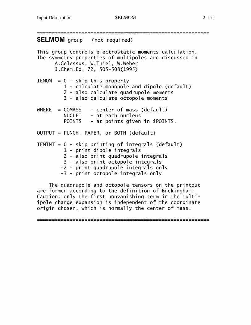
Input Description $ELMOM 2-151
==========================================================
$ELMOM group (not required)
This group controls electrostatic moments calculation.The symmetry properties of multipoles are discussed in A.Gelessus, W.Thiel, W.Weber J.Chem.Ed. 72, 505-508(1995)
IEMOM = 0 - skip this property 1 - calculate monopole and dipole (default) 2 - also calculate quadrupole moments 3 - also calculate octopole moments
WHERE = COMASS - center of mass (default) NUCLEI - at each nucleus POINTS - at points given in $POINTS.
OUTPUT = PUNCH, PAPER, or BOTH (default)
IEMINT = 0 - skip printing of integrals (default) 1 - print dipole integrals 2 - also print quadrupole integrals 3 - also print octopole integrals -2 - print quadrupole integrals only -3 - print octopole integrals only
The quadrupole and octopole tensors on the printoutare formed according to the definition of Buckingham.Caution: only the first nonvanishing term in the multi-ipole charge expansion is independent of the coordinateorigin chosen, which is normally the center of mass.
==========================================================
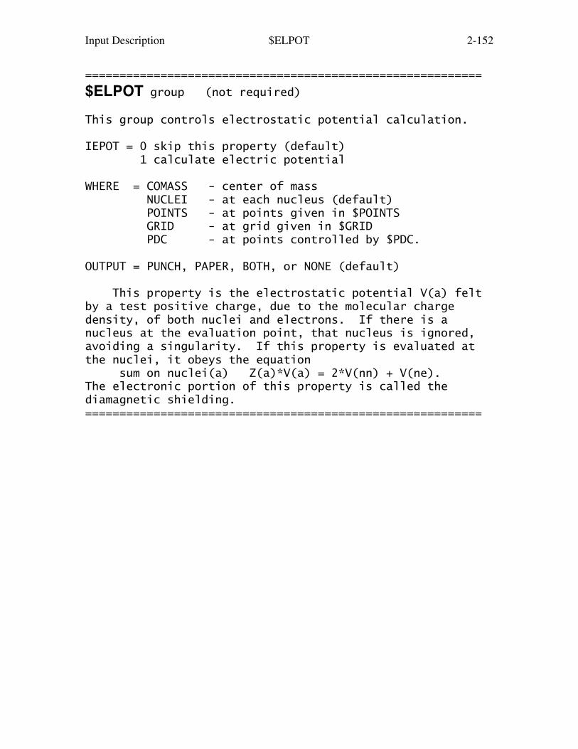
Input Description $ELPOT 2-152
==========================================================
$ELPOT group (not required)
This group controls electrostatic potential calculation.
IEPOT = 0 skip this property (default) 1 calculate electric potential
WHERE = COMASS - center of mass NUCLEI - at each nucleus (default) POINTS - at points given in $POINTS GRID - at grid given in $GRID PDC - at points controlled by $PDC.
OUTPUT = PUNCH, PAPER, BOTH, or NONE (default)
This property is the electrostatic potential V(a) feltby a test positive charge, due to the molecular chargedensity, of both nuclei and electrons. If there is anucleus at the evaluation point, that nucleus is ignored,avoiding a singularity. If this property is evaluated atthe nuclei, it obeys the equation sum on nuclei(a) Z(a)*V(a) = 2*V(nn) + V(ne).The electronic portion of this property is called thediamagnetic shielding.==========================================================

Input Description $ELDENS 2-153
==========================================================
$ELDENS group (not required)
This group controls electron density calculation.
IEDEN = 0 skip this property (default) = 1 compute the electron density.
MORB = The molecular orbital whose electron density is to be computed. If zero, the total density is computed. (default=0)
WHERE = COMASS - center of mass NUCLEI - at each nucleus (default) POINTS - at points given in $POINTS GRID - at grid given in $GRID
OUTPUT = PUNCH, PAPER, or BOTH (default)
IEDINT = 0 - skip printing of integrals (default) 1 - print the electron density integrals
==========================================================
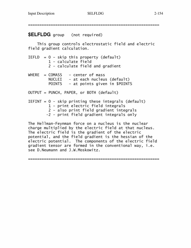
Input Description $ELFLDG 2-154
==========================================================
$ELFLDG group (not required)
This group controls electrostatic field and electricfield gradient calculation.
IEFLD = 0 - skip this property (default) 1 - calculate field 2 - calculate field and gradient
WHERE = COMASS - center of mass NUCLEI - at each nucleus (default) POINTS - at points given in $POINTS
OUTPUT = PUNCH, PAPER, or BOTH (default)
IEFINT = 0 - skip printing these integrals (default) 1 - print electric field integrals 2 - also print field gradient integrals -2 - print field gradient integrals only
The Hellman-Feynman force on a nucleus is the nuclearcharge multiplied by the electric field at that nucleus.The electric field is the gradient of the electricpotential, and the field gradient is the hessian of theelectric potential. The components of the electric fieldgradient tensor are formed in the conventional way, i.e.see D.Neumann and J.W.Moskowitz.
==========================================================

Input Description $POINTS $GRID 2-155
==========================================================
$POINTS group (not required)
This group is used to input points at which propertieswill be computed. This first card in the group mustcontain the string ANGS or BOHR, followed by an integerNPOINT, the number of points to be used. The next NPOINTcards are read in free format, containing the X, Y, and Zcoordinates of each desired point.
==========================================================
$GRID group (not required)
This group is used to input a grid (plane through themolecule) on which properties will be calculated.
ORIGIN(i) = coordinates of the lower left corner of the plot.XVEC(i) = coordinates of the lower right corner of the plot.YVEC(i) = coordinates of the upper left corner of the plot.SIZE = grid increment, default is 0.25.UNITS = units of the above four values, it can be either BOHR or ANGS (the default).
Note that XVEC and YVEC are not necessarily parallel tothe X and Y axes, rather they are the axes which youdesire to see plotted by the MEPMAP contouring program.
==========================================================
* * * * * * * * * * * * * * * * * * * * For conversion factors, and references see the 'further information' section. * * * * * * * * * * * * * * * * * * * *
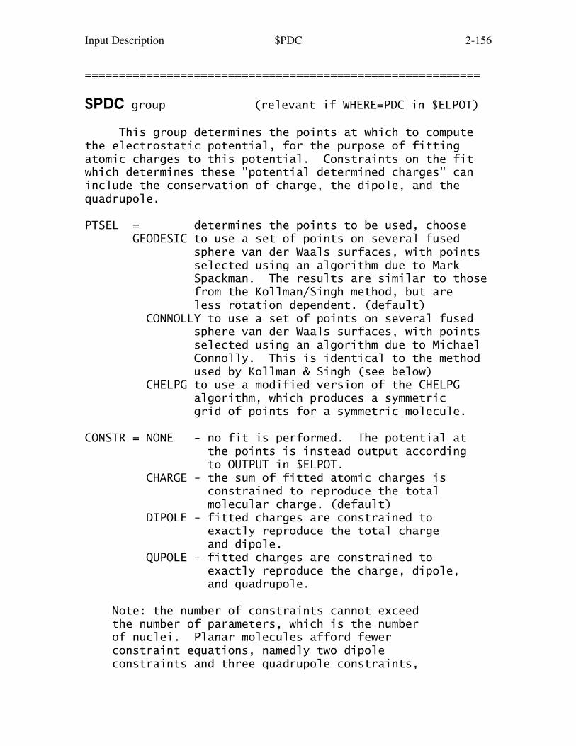
Input Description $PDC 2-156
==========================================================
$PDC group (relevant if WHERE=PDC in $ELPOT)
This group determines the points at which to computethe electrostatic potential, for the purpose of fittingatomic charges to this potential. Constraints on the fitwhich determines these "potential determined charges" caninclude the conservation of charge, the dipole, and thequadrupole.
PTSEL = determines the points to be used, choose GEODESIC to use a set of points on several fused sphere van der Waals surfaces, with points selected using an algorithm due to Mark Spackman. The results are similar to those from the Kollman/Singh method, but are less rotation dependent. (default) CONNOLLY to use a set of points on several fused sphere van der Waals surfaces, with points selected using an algorithm due to Michael Connolly. This is identical to the method used by Kollman & Singh (see below) CHELPG to use a modified version of the CHELPG algorithm, which produces a symmetric grid of points for a symmetric molecule.
CONSTR = NONE - no fit is performed. The potential at the points is instead output according to OUTPUT in $ELPOT. CHARGE - the sum of fitted atomic charges is constrained to reproduce the total molecular charge. (default) DIPOLE - fitted charges are constrained to exactly reproduce the total charge and dipole. QUPOLE - fitted charges are constrained to exactly reproduce the charge, dipole, and quadrupole.
Note: the number of constraints cannot exceed the number of parameters, which is the number of nuclei. Planar molecules afford fewer constraint equations, namedly two dipole constraints and three quadrupole constraints,
Input Description $PDC 2-157
instead of three and five, repectively.
* * the next 5 pertain to PTSEL=GEODESIC or CONNOLLY * *
VDWSCL = scale factor for the first shell of VDW spheres. The default of 1.4 seems to be an empirical best value. Values for VDW radii for most elements up to Z=36 are internally stored.
VDWINC = increment for successive shells (default = 0.2). The defaults for VDWSCL and VDWINC will result in points chosen on layers at 1.4, 1.6, 1.8 etc times the VDW radii of the atoms.
LAYER = number of layers of points chosen on successive fused sphere VDW surfaces (default = 4)
Note: RUNTYP=MAKEFP's screening calculation changes thedefaults to VDWSCL=0.5 or 0.8 depending on the type ofStone analysis, VDWINC=0.1, LAYER=25, and MAXPDC=100,000.
NFREQ = flag for particular geodesic tesselation of points. Only relevant if PTSEL=GEODESIC. Options are: (10*h + k) for {3,5+}h,k tesselations -(10*h + k) for {5+,3}h,k tesselations Of course both nh and nk must be less than 10, so NFREQ must lie within the range -99 to 99. The default value is NFREQ=30 (=03)
PTDENS = density of points on the surface of each scaled VDW sphere (in points per square au). Relevant if PTSEL=CONNOLLY. Default=0.28 per au squared, which corresponds to 1.0 per square Angstrom, the default recommended by Kollman & Singh.
* * * the next two pertain to PTSEL=CHELPG * * *
RMAX = maximum distance from any point to the closest atom. (default=3.0 Angstroms)
DELR = distance between points on the grid. (default=0.8 Angstroms)
Input Description $PDC 2-158
MAXPDC = an estimate of the total number of points whose electrostatic potential will be included in the fit. (default=10000)
CENTER = an array of coordinates at which the moments were computed.
DPOLE = the molecular dipole.
QPOLE = the molecular quadrupole.
PDUNIT = units for the above values. ANGS (default) will mean that the coordinates are in Angstroms, the dipole in Debye, and quadrupole in Buckinghams. BOHR implies atomic units for all 3.
Note: it is easier to compute the moments in the current run, by setting IEMOM to at least 2 in $ELMOM. However, you could fit experimental data, for example, by reading it in here.
==========================================================
There is no unique way to define fitted atomiccharges. Smaller numbers of points at which the electro-static potential is fit, changes in VDW radii, asymmetricpoint location, etc. all affect the results. A usefulbibliography is
U.C.Singh, P.A.Kollman, J.Comput.Chem. 5, 129-145(1984)L.E.Chirlain, M.M.Francl, J.Comput.Chem. 8, 894-905(1987)R.J.Woods, M.Khalil, W.Pell, S.H.Moffatt, V.H.Smith, J.Comput.Chem. 11, 297-310(1990)C.M.Breneman, K.B.Wiberg, J.Comput.Chem. 11, 361-373(1990)K.M.Merz, J.Comput.Chem. 13, 749(1992)M.A.Spackman, J.Comput.Chem. 17, 1-18(1996)
Start your reading with the last paper shown.

Input Description $RADIAL 2-159
==========================================================
$RADIAL group (relevant only to atoms)
This input data governs the computation of radialexpectation values <r> and <r**2> for atomic orbitals. Theatomic wavefunctions can be any SCFTYP except UHF. Theatomic calculation should preserve radial degeneracy in p,d, or f shells, so UHF is not allowed, and furthermore,many atoms will require GVB or MCSCF inputs (see the'Further References' section about doing atomic SCF). Itis OK to use core potentials (MCP or ECP) or to applyscalar relativistic effects, so long as the calculationpreserves degeneracy 2l+1 in every occupied shell.
One should keep in mind that there is some arbitrarinessin how different SCFTYPs canonicalize orbitals, so thatindividual orbitals may vary, for exactly the same totalwavefunction. For example, ROHF orbitals within the doublyoccupied set of orbitals change as a function of the A andB canonicalization inputs (see 'Further References').Similar comments apply to orbitals from GVB or MCSCF.
It is recommended that you do two runs, first to checkif radial degeneracy is maintained (equal eigenvalues forall three p, or all five d orbitals). This preliminary runwill help count which orbitals lie in degenerate shells,for MEMSH below. The quality of the numerical radialintegration can be assessed from its closeness to 1.0.Radial wavefunctions can be printed, as an option. Thereare no defaults provided for the first three keywords,which are required inputs, if this group is given.
NSHELL - number of atomic shells to be computed
IDEGSH - an array of NSHELL values, giving the degeneracy of each shell (1, 3, 5, or 7)
MEMSH - an array containing the sum of all IDEGSH values, listing the members of each shell.
RMAX - maximum radius to be considered, in Bohr. The default is most appropriate for valence orbitals, which for bottom row elements may extend to five Angstrons (default=10.0). Inner shell orbitals
Input Description $RADIAL 2-160
may require input of a smaller RMAX, to move some of the tick marks closer to the nucleus.
NTICKS - radial increment is RMAX/NTICKS, so the default step size is 0.01 Bohr (default NTICKS=1001)
PRTRAD - flag to print each shell's radial wavefunction at every radial tick mark (default is .FALSE.)
The following example uses a basis that is too small to beconverged, printing radial expectation values for manganeseas 1s=0.0615, 3p=0.9156, 4s=3.4027, and 3d=1.1095:
$contrl scftyp=rohf mult=6 ispher=1 $end $guess guess=huckel norder=1 iorder(10)=15,10,11,12,13,14 $end $basis gbasis=n31 ngauss=6 $end $scf rstrct=.true. $end $radial nshell=4 idegsh(1)=1,3,1,5 memsh(1)=1, 7,8,9, 10, 11,12,13,14,15 $end $dataMn atom...(4s)2(3d)5...6-S...spherical harmonicsDnh 2
Mn 25.0 $end
==========================================================
Input Description $MOLGRF 2-161
==========================================================
$MOLGRF group (relevant only if you have MOLGRAPH)
This option provides an interface for viewing orbitalsthrough a commercial package named MOLGRAPH, from DaikinIndustries. Note that this option uses three disk fileswhich are not defined in the GAMESS execution scripts weprovide, since we don't use MOLGRAPH ourselves. You willneed to define files 28, 29, 30, as generic names PRGRID,COGRID, MOGRID, of which the latter is passed to MOLGRAPH.
GRID3D = a flag to generate 3D grid data. (default is .false.).
TOTAL = a flag to generate a total density grid data. "Total" means the sum of the orbital densities given by NPLT array. (default is .false.).
MESH = numbers of grids. You can use different numbers for three axes. (default is MESH(1)=21,21,21).
BOUND = boundary coordinates of a 3D graphical cell. The default is that the cell is larger than the molecular skeleton by 3 bohr in all directions. E.g., BOUND(1)=xmin,xmax,ymin,ymax,zmin,zmax
NPLOTS = number of orbitals to be used to generate 3D grid data. (default is NPLOTS=1).
NPLT = orbital IDs. The default is 1 orbital only, the HOMO or SOMO. If the LOCAL option is given in $CONTRL, localized orbital IDs should be given. For example, NPLT(1)=n1,n2,n3,...
CHECK = debug option, printing some of the grid data.
If you are interested in graphics, look at the GAMESS webpage for information about other graphics packages withGAMESS, particularly MacMolPlt and Avogadro, both areavailable for all common desktop operating systems.
==========================================================

Input Description $STONE 2-162
==========================================================
$STONE group (optional)
This group defines the expansion points for Stone'sdistributed multipole analysis (DMA) of the electrostaticpotential.
The DMA takes the multipolar expansion of each overlapcharge density defined by two Gaussian primitives, andtranslates it from the center of charge of the overlapdensity to the nearest expansion point. Some referencesfor the method are
A.J.Stone Chem.Phys.Lett. 83, 233-239 (1981) A.J.Stone, M.Alderton Mol.Phys. 56, 1047-1064(1985) A.J.Stone J.Chem.Theory and Comput. 1, 1128-1132(2005)
The existence of a $STONE group in the input is whattriggers the analysis. The first set of lines must appearas the first line after $STONE (enter a blank line if youmake no choice), then enter as many choices as you wish, inany order, from the other sets.
----------------------------------------------------------
BIGEXP <value> exponents larger than this are treated by the original Stone expansion, and those smaller by a numerical integration. The default is 0.0, meaning no numerical grid. The other parameters are meaningless if BIGEXP remains zero.
NRAD <nrad> number of radial grid points (default 100)NANG <nang> number of angular grid points, choose one of the Lebedev grid values (default 590)SMOOTH <nbecke> degree of Becke smoothing (default=2)SMRAD <nbckrd> Radii choice, 0=constant, 1=Bragg-Slater, which is the default.
----------------------------------------------------------
ATOM i name, where
ATOM is a keyword indicating that a particular
Input Description $STONE 2-163
atom is selected as an expansion center. i is the number of the atom name is an optional name for the atom. If not entered the name will be set to the name used in the $DATA input.
----------------------------------------------------------
ATOMS is a keyword selecting all nuclei in the molecule as expansion points. No other input on the line is necessary.
----------------------------------------------------------
BONDS is a keyword selecting all bond midpoints in the molecule as expansion points. No other input on the line is necessary.
----------------------------------------------------------
BOND i j name, where
BOND is a keyword indicating that a bond mid- point is selected as an expansion center. i,j are the indices of the atoms defining the bond, corresponding to two atoms in $DATA. name an optional name for the bond midpoint. If omitted, it is set to 'BOND'.
----------------------------------------------------------
CMASS is a keyword selecting the center of mass as an expansion point. No other input on the line is necessary.
----------------------------------------------------------
POINT x y z name, where
POINT is a keyword indicating that an arbitrary point is selected as an expansion point. x,y,z are the coordinates of the point, in Bohr. name is an optional name for the expansion point. If omitted, it is set to 'POINT'.
Input Description $STONE 2-164
----------------------------------------------------------
While making the EFPs for QM/MM run, a single keywordQMMMBUF is necessary. Adding additional keywords may leadto meaningless results. The program will automaticallyselect atoms and bond midpoints which are outside thebuffer zone as the multipole expansion points.
QMMMBUF nmo, where
QMMMBUF is a keyword specifying the number of QM/MM buffer molecular orbitals, which must be the first NMO orbitals in the MO set. These orbitals must be frozen in the buffer zone, so this is useful only if $MOFRZ is given. NMO is the number of buffer MO-s (if NMO is omitted, it will be set to the number of frozen MOs in $MOFRZ)
==========================================================
The second and third moments on the printout can beconverted to Buckingham's tensors by formula 9 of A.D.Buckingham, Quart.Rev. 13, 183-214 (1959)These can in turn be converted to spherical tensorsby the formulae in the appendix of S.L.Price, et al. Mol.Phys. 52, 987-1001 (1984)

Input Description $RAMAN 2-165
==========================================================
$RAMAN group (relevant for all SCFTYPs)
This input controls the computation of Raman intensityby the numerical differentiation produre of Komornicki andothers. It is applicable to any wavefunction for whichthe analytic gradient is available, including some MP2 andCI cases. The calculation involves the computation of 19nuclear gradients, one without applied electric fields,plus 18 no symmetry runs with electric fields applied invarious directions. The numerical second differencingproduces intensity values with 2-3 digits of accuracy.
This run must follow an earlier RUNTYP=HESSIAN job,and the $GRAD and $HESS groups from that first job must begiven as input. If the $DIPDR is computed analyticallyby this Hessian job, it too may be read in, if not, thenumerical Raman job will evaluate $DIPDR. Once the datafrom the 19 applied fields is available, the $ALPDR tensoris evaluated. Then the nuclear derivatives of the dipolemoment and alpha polarizability will be combined with thenormal coordinate information to produce the IR and Ramanintensity of each mode.
To study isotopic substitution speedily, input the$GRAD, $HESS, $DIPDR, and $ALPDR groups along with thedesired atomic masses in $MASS.
The code does not permit semi-empirical or solvationmodels to be used.
EFIELD = applied electric field strenth. The literature suggests values in the range 0.001 to 0.005. (default = 0.002 a.u.)
==========================================================
Input Description $ALPDR 2-166
==========================================================
$ALPDR group (relevant for RUNTYP=RAMAN or HESSIAN)
Formatted alpha derivative tensor, punched by a previousRUNTYP=RAMAN job. If both $DIPDR and this group are foundin the input file, the applied field computation will beskipped, to immediately evaluate IR and Raman intensities.
If this group is found during RUNTYP=HESSIAN, the Ramanintensities will be added to the output. You might wantto run as RUNTYP=HESSIAN instead of RUNTYP=RAMAN in orderto have access to PROJCT or the other options available inthe $FORCE group.
==========================================================
Input Description $NMR 2-167
==========================================================
$NMR group (optional, relevant if RUNTYP=NMR)
This group governs the analytic computation of the NMRshielding tensor for each nucleus, using the GaugeInvariant Atomic Orbital (GIAO) method, also known asLondon orbitals. The most useful input values are thefirst three printing options. The wavefunction must beRHF, the atomic basis set may be spdfg, the EFP model maybe used to include solvent effects, and the McMurchie-Davidson integrals used are not fast.
ANGINT = a flag to control the evaluation of the perturbed two-electron integrals by increasing the angular momentum on the unperturbed 2e- integrals. With this selected, only two passes through the 2e- NMR integral code are needed. Otherwise, six slow passes are needed, and option meant only for debugging purposes. (default=.TRUE.)
INMEM A flag to carry all integrals in memory. If selected, the calculation will require several multiples of NAO**4. By default, the calculation will require space on the order of NATOMS*NAO**2, where NAO is the basis set dimension. This is useful for debugging. (default=.FALSE.)
The rest are print flags, in increasing order of the amountof output created, as well as decreasing order of interest.The default for all of these options is .FALSE.
PDIA Print diamagnetic term of the shielding tensor.
PPARA Print paramagnetic term of the shielding tensor.
PEVEC Print eigenvectors of asymmetric shielding tensor.
PITER Print iteration data for the formation of the three first-order density matrices.
PRMAT Print the three first-order perturbed density matrices, the three first-order H matrices for

Input Description $NMR 2-168
each nucleus, the unperturbed density matrix, and the nine second-order H matrices for each nucleus.
POEINT Print all one-electron integrals.
PTEINT Print the perturbed two-electron integrals.
TEDBG Print VAST amounts of debugging information for the McMurchie-Davidson two-electron intgrals. Should only be used for the smallest test jobs.
==========================================================
Input Description $MOROKM 2-169
==========================================================
$MOROKM group (relevant if RUNTYP=EDA)
This performs an analysis of the energy contributionsto dimerization (or formation of larger clusters),according to the Morokuma-Kitaura and/or ReducedVariational Space schemes. The analysis is limited toclosed shell RHF monomers. See also the $LMOEDA inputgroup for more general energy decompositions. See alsoPIEDA in the FMO codes.
Solvation models are not supported.
MOROKM = a flag to request Morokuma-Kitaura decomposition. (default is .TRUE.)
RVS = a flag to request "reduced variation space" decomposition. This differs from the Morokuma analysis. One or the other or both may be requested in the same run. (default is .FALSE.)
Generally speaking, RVS handles non-orthogonality ofmonomers better. When diffuse functions are used, theMOROKM analysis sometimes fails, but RVS will work.
BSSE = a flag to request basis set superposition error be computed. You must ensure that CTPSPL is selected. This option applies only to MOROKM decompositions, as a basis superposition error is automatically generated by the RVS scheme. This is not the full Boys counterpoise correction, as explained in the reference. (default is .FALSE.)
* * *
The inputs here control how the RHF supermolecule, whosecoordinates are given in the $DATA group, is divided intotwo or more monomers.
IATM = An array giving the number of atoms in each of the monomer. Up to ten monomers may be defined. Your input in $DATA must have all the atoms in the first monomer defined before the atoms in the second monomer, before the third monomer... The
Input Description $MOROKM 2-170
number of atoms belonging to the final monomer can be omitted. There is no sensible default for IATM, so don't omit it from your input.
ICHM = An array giving the charges of the each monomer. The charge of the final monomer may be omitted, as it is fixed by ICH in $CONTRL, which is the total charge of the supermolecule. The default is neutral monomers, ICHM(1)=0,0,0,...
EQUM = a flag to indicate all monomers are equivalent by symmetry (in addition to containing identical atoms). If so, which is not often true, then only the unique computations will be done. (default is .FALSE.)
* * *
CTPSPL = a flag to decompose the interaction energy into charge transfer plus polarization terms. This is most appropriate for weakly interacting monomers. (default is .TRUE.)
CTPLX = a flag to combine the CT and POL terms into a single term. If you select this, you might want to turn CTPSPL off to avoid the extra work that that decomposition entails, or you can analyze both ways in the same run. (default is .FALSE.)
RDENG = a flag to enable restarting, by reading the lines containing "FINAL ENERGY" from a previous run. The $EMORO group is single lines read under format A16,F20.10 containing the energies, and a card $END to complete. The 16 chars = anything. (default is .FALSE.)
==========================================================
The present implementation has some quirks:
1. The initial guess of the monomer orbitals is notcontrolled by $GUESS. The program first looks for a $VEC1,$VEC2, ... group for each monomer. The orbitals must beobtained for the identical coordinates which that monomerhas within the supermolecule. If any $VECn groups are
Input Description $MOROKM 2-171
found, they will be MOREAD. If any are missing, the guessfor that monomer will be constructed by HCORE. Check yourmonomer energies carefully! The initial guess orbitals forthe supermolecule are formed from a block diagonal matrixcontaining the monomer orbitals.2. The use of symmetry is turned off internally.3. Spherical harmonics (ISPHER=1) may not be used.4. There is no direct SCF option. File ORDINT will be afull C1 list of integrals. File AOINTS will containwhatever subset of these is needed for each particulardecomposition step. So extra disk space is needed comparedto RUNTYP=ENERGY.5. This run type applies only to ab initio RHF treatment ofthe monomers. To be quite specific: this means that DFT(which involves a grid, not just integrals) will not work,nor will MOPAC's approximated 2e- integrals6. This kind of calculation will run in parallel.
Quirks 1, 3 and 4 can be eliminated by using PIEDA if onlytwo monomers are present. For more monomers PIEDA resultswill slightly differ. PIEDA is a special case of FMO, q.v.
References:
C.Coulson in "Hydrogen Bonding", D.Hadzi, H.W.Thompson, Eds., Pergamon Press, NY, 1957, pp 339-360.C.Coulson Research, 10, 149-159 (1957).K.Morokuma J.Chem.Phys. 55, 1236-44 (1971).K.Kitaura, K.Morokuma Int.J.Quantum Chem. 10, 325 (1976).K.Morokuma, K.Kitaura in "Chemical Applications of Electrostatic Potentials", P.Politzer,D.G.Truhlar, Eds. Plenum Press, NY, 1981, pp 215-242.The method coded is the newer version described in the 1976and 1981 papers. In particular, note that the CT term iscomputed separately for each monomer, as described in thewords below eqn. 16 of the 1981 paper, not simultaneously.
Reduced Variational Space:W.J.Stevens, W.H.Fink, Chem.Phys.Lett. 139, 15-22(1987).
A comparison of the RVS and Morokuma decompositions can befound in the review article: "Wavefunctions and ChemicalBonding" M.S.Gordon, J.H.Jensen in "Encyclopedia ofComputational Chemistry", volume 5, P.V.R.Schleyer, editor,John Wiley and Sons, Chichester, 1998.
Input Description $MOROKM 2-172
BSSE during Morokuma decomposition:R.Cammi, R.Bonaccorsi, J.TomasiTheoret.Chim.Acta 68, 271-283(1985).
The present implementation:"Energy decomposition analysis for many-body interactions, and application to water complexes"W.Chen, M.S.Gordon J.Phys.Chem. 100, 14316-14328(1996)

Input Description $LMOEDA 2-173
==========================================================
$LMOEDA group (relevant if RUNTYP=EDA)
This group governs the Localized Molecular OrbitalEnergy Decomposition Analysis, which is capable of moresophisticated treatment of "monomers" than the Morokuma orRVS schemes (see $MOROKM). For example, the wavefunctionsof the monomers may be RHF, ROHF, or UHF, the DFTcounterparts of each of these, the MP2 counterparts of eachof these, or CCSD and CCSD(T) for RHF and ROHF references.Furthermore, division of the system into "monomers" caninvolve splitting chemical bond pairs, as the MMULT examplebelow shows.
If one or more monomers are open shell, to be treatedby ROHF, use SCFTYP=ROHF in $CONTRL. Whenever a monomerhas an even number of electrons, so that its MMULT=1 below,SCFTYP=ROHF (or UHF) automatically reduces to RHF on thatmonomer.
MATOM = an array giving the number of atoms in each monomer. Up to ten monomers may be defined. Your input in $DATA must have all the atoms in the first monomer defined before the atoms in the second monomer, before the third monomer etc. The sum of the MATOM array must be equal to the total number in the supermolecule.
MCHARG = an array giving the charge of each monomer. Up to ten monomers may be defined. The sum of the charges in the monomers must be equal to the total charge of the supermolecule.
MMULT = an array giving the multiplicity of each monomer. Up to ten monomers may be defined. A positive integer means alpha spin, a negative integer means beta spin. For example, if an ethane molecule is separated into two neutral CH3 groups, MMULT(1)=2,-2 or MMULT(1)=-2,2.
SUPBAS = a flag to request Boys and Bernardi style counterpoise method for correcting basis set superposition errors. (default is .FALSE.).

Input Description $LMOEDA 2-174
Usually it works well with Hartree-Fock and MP2 and coupled cluster methods, but less well with DFT methods due to SCF divergent problems.
A paper describing this method is currently under review.
==========================================================
Input Description $FFCALC 2-175
==========================================================
$FFCALC group (relevant for RUNTYP=FFIELD)
This group permits the study of the influence of anapplied electric field on the wavefunction. The mostcommon finite field calculation applies a sequence offields to extract the linear polarizability and the firstand second order hyperpolarizabilities (static alpha, beta,and gamma tensors). The method is general, because itrelies on finite differencing of the energy values, and soworks for all ab initio wavefunctions. If the dipolemoments are available (true for SCF or CI functions, andsee MPPROP in $MP2), the same tensors are formed bydifferencing the dipoles, which is more accurate. Someidea of the error in the numerical differentiations can begleaned by comparing energy based and dipole basedquantities.
For analytic computation of static polarizabilitiesalpha, beta, and gamma (as well as frequency dependent NLOproperties), for closed shell cases, see $TDHF and $TDHFX.For analytic computation of the static polarizabilityalpha, see POLAR in $CPHF.
The standard computation obtains the polarizabilities,by double numerical differentiation. See ONEFLD to apply asingle electric field, but for a more general approach toapplied static fields, see $EFIELD.
OFFDIA = .TRUE. computes the entire polarizability tensors, which requires a total of 49 wavefunction evaluations (some of gamma is not formed). = .FALSE. forms only diagonal components of the polarizabilities, using 19 wavefunctions. The default is .FALSE.
ESTEP = step size for the applied electric field strength, 0.01 to 0.001 is reasonable. (default=0.001 a.u.)
The next parameters pertain to applying a field in only onedirection:
Input Description $FFCALC 2-176
ONEFLD = flag to apply one field (default=.FALSE.)
SYM = a flag to specify when the field to be applied does not break the molecular symmetry. Since most fields do break the nuclear point group symmetry, the default is .FALSE.
EFIELD = an array of the three x,y,z components of the single applied field.
LOCHYP = a flag to perform a localized orbital analysis of the alpha, beta, and gamma polarizabilities. See $LOCAL for similar analyses of the energy, multipole moments, or alpha tensor. References for this keyword are given below.
Finite field calculations require large basis sets, andextraordinary accuracy in the wavefunction. To convergethe SCF to many digits is sometimes problematic, but wesuggest you use the input to increase integral accuracy andwavefunction convergence, for example
$CONTRL ICUT=20 ITOL=30 $END $SCF CONV=1d-7 FDIFF=.FALSE. $END
Examples of fields that do not break symmetry are a Z-axis field for an axial point group which is notcentrosymmetric (i.e. C2v). However, a field in the X or Ydirection does break the C2v symmetry. Application of a Z-axis field for benzene breaks D6h symmetry. However, youcould enter the group as C6v in $DATA while using D6hcoordinates, and regain the prospect of using SYM=.TRUE.If you wanted to go on to apply a second field for benzenein the X direction, you might want to enter Cs in $DATA,which will necessitate the input of two more carbon andhydrogen atom, but recovers use of SYM=.TRUE.
References: J.E.Gready, G.B.Bacskay, N.S.Hush Chem.Phys. 22, 141-150(1977) H.A.Kurtz, J.J.P.Stewart, K.M.Dieter J.Comput.Chem. 11, 82-87(1990).

Input Description $FFCALC 2-177
polarizability analysis: S.Suehara, P.Thomas, A.P.Mirgorodsky, T.Merle-Mejean, J.C.Champarnaud-Mesjard, T.Aizawa, S.Hishita, S.Todoroki, T.Konishi, S.Inoue Phys.Rev.B 70, 205121/1-7(2004) S.Suehara, T.Konishi, S.Inoue Phys.Rev.B 73, 092203/1-4(2006)
==========================================================
Input Description $TDHF 2-178
==========================================================
$TDHF group (relevant for SCFTYP=RHF if RUNTYP=TDHF)
This group permits the analytic calculation of variousstatic and/or frequency dependent polarizabilities, with anemphasis on important NLO properties such as second andthird harmonic generation. The method is programmed onlyfor closed shell wavefunctions, at the semi-empirical or abinitio level. Ab initio calculations may be direct SCF, orparallel, if desired, except INIG=2.
Because the Fock matrices computed during the time-dependent Hartree-Fock CPHF are not symmetric, you may notuse symmetry. You must enter NOSYM=1 in $CONTRL!
For a more general numerical approach to the staticproperties, see $FFCALC. For additional closed shelldynamic polarizabilities and spectra, see $TDHFX.
NFREQ = Number of frequencies to be used. (default=1)
FREQ = An array of energy values in atomic units. For example: if NFREQ=3 then FREQ(1)=0.0,0.1,0.25. By default, only the static polarizabilities are computed. (default is freq(1)=0.0)
The conversion factor from wavenumbers to Hartree is to divide by 219,474.6. To convert a wavelength to Hartree, compute FREQ=45.56/lamda, lambda in nm.
MAXITA = Maximum number of iterations for an alpha computation. (default=100)
MAXITU = Maximum number of iterations in the second order correction calculation. This applies to iterative beta values and all gammas. (default=100)
ATOL = Tolerance for convergence of first-order results. (default=1.0d-05)
BTOL = Tolerance for convergence of second-order results. (default=1.0d-05)

Input Description $TDHF 2-179
RETDHF = a flag to choose starting points for iterative calculations from best previous results. (default=.true.)
* * * the following NLO properties are available * * *
alpha polarizabilities are always calculated.
INIB = 0 turns off all beta computation (default) = 1 calculates only noniterative beta = 2 calculate iterative and noniterative beta The next flags allow further BETA tuning
BSHG = Calculate beta for second harmonic generation.
BEOPE = Calculate beta for electrooptic Pockels effect.
BOR = Calculate beta for optical rectification.
INIG = 0 turns off all gamma computation (default) = 1 calculates only noniterative gamma = 2 calculate iterative and noniterative gamma The next flags allow further GAMMA tuning
GTHG = Calculate gamma for third harmonic generation.
GEFISH = Calculate gamma for electric-field induced second harmonic generation.
GIDRI = Calculate gamma for intensity dependent refractive index.
GOKE = Calculate gamma for optical Kerr effect.
These will be computed only if a nonzero energy (FREQ)is requested. The default for each flag is .TRUE., andthey may be turned off individually by setting some .FALSE.Note however that the program determines the best way tocalculate them. For example, if you wish to have the SHGresults but no gamma results are needed, the SHG beta willbe computed in a non-iterative way from alpha(w) andalpha(2w). However if you request the computation of theTHG gamma, the second order U(w,w) results are needed and
Input Description $TDHF 2-180
an iterative SHG calculation will be performed whether yourequest it or not, as it is a required intermediate.
Only the following combinations make sense: INIB INIG giving FREQ(1)=0.0,0.1 e.g. w=0.1 0 0 static alpha, a(w) 1 0 static alpha,beta a(w),a(2w) noniterative b(OR), b(EOPE), b(SHG) 2 0 static alpha,beta a(w),a(2w) noniterative b(OR), b(EOPE), b(SHG) iterative b(OR), b(EOPE), b(SHG) 2 1 static alpha,beta,gamma a(w),a(2w) iterative b(OR), b(EOPE), b(SHG) noniterative g(THG), g(EFISH), g(IDRI), g(OKE) 2 2 static alpha,beta,gamma a(w),a(2w) iterative b(OR), b(EOPE), b(SHG) noniterative g(THG), g(EFISH), g(IDRI), g(OKE) iterative static gamma, g(OKE), g(THG), g(EFISH), g(IDRI), g(DC-OR)
This is a quirky program:
1. INIG=2 only runs in serial, and only runs with AOintegrals on disk.2. ISPHER=1 may not be chosen.3. INIB=1 and INIB=2 print the same components for OR, OPE,SHG, but different totals from the whole tensor. It is notclear which is correct.4. units are not well specified on the output!
References:for static polarizabilities,G.J.B.Hurst, M.Dupuis, E.Clementi J.Chem.Phys. 89, 385-395(1988)for dynamic polarizabilities,S.P.Karna, M.Dupuis J.Comput.Chem. 12, 487-504 (1991).P.Korambath, H.A.Kurtz, in "Nonlinear Optical Materials",ACS Symposium Series 628, S.P.Karna and A.T.Yeates, Eds.pp 133-144, Washington DC, 1996.Review: D.P.Shelton, J.E.Rice, Chem.Rev. 94, 3-29(1994).
==========================================================
Input Description $TDHFX 2-181
==========================================================
$TDHFX group (relevent for SCF=RHF if RUNTYP=TDHFX)
This group permits the analytical determination ofstatic and/or frequency dependent polarizabilities andhyperpolarizabilities (alpha, beta, and gamma), as well astheir first- and second-order geometrical derivatives (ofalpha and beta). This permits the prediction of dynamic(nonresonant) Raman and hyper-Raman spectra, yielding bothintensities and depolarizations. The method is onlyavailable for closed shell systems (RHF).
For other polarizability options, see $FFCALC and $TDHF.For ordinary Raman spectra, see $RAMAN.
You must not use point group symmetry in this kind ofcalculation (except to enter the molecule's structure), soprovide NOSYM=1. Since the derivative level is quite high,it is a good idea to converge the SCF problem crisply,CONV=1.0D-6. These options are not forced by the RUNTYP,so please use explicit input.
The $TDHFX group acts as a script. Each keyword must beon a separate line, terminated by a $END. The availablekeywords are gathered into 3 sets. Those belonging to thefirst set must appear before the second set, which mustappear before the third set.
Set 1:
Here is a list of keywords that specifies the number ofparameters (electric fields and geometrical distortions)that will be taken into account in the computations.
ALLDIRS = compute the responses for all the electric field directions (x,y,z).
DIR idir = compute the responses for one electric field specific direction: x(idir=1), y(idir=2) and z(idir=3).
USE_C = do the computation in Cartesian coordinates.
USE_Q = do the computation in normal coordinates.

Input Description $TDHFX 2-182
The default is ALLDIRS and USE_C.
Set 2:
The following two keywords must be specified before anycomputation that requires vibrational frequencies or normalmodes of vibration:
FREQ = compute the normal modes and the harmonic vibrational frequencies. Do a HESSIAN job.
FREQ2 = same as FREQ but store the second derivative of the monoelectronic Hamiltonian. Required if you want to determine geometrical second-order derivatives of properties.
Set 3:
The following keywords are related to the generalizediterative method to solve TDHF mixed derivative equations.They can be inserted anywhere in the $TDHFX group andchange the behavior of the generalized iterative method forany of the following tasks that might be requested.
DIIS = Use the DIIS method. This is the default method.
NOACCEL = Do not use any accelerating method.
ITERMAX imax = Specify the maximum number of iterations to obtain the converged solution. Default=100.
CONV threshold = the threshold convergence criterion for the U response matrices. Default=1E-5.
Below are the keywords to select a particular computation.The xx_NI version will call a non-iterative procedure.
The laser energy (w) must be given in Hartree. Divide by219,474.6 to convert a frequency in wavenumbers (cm-1) to aphoton energy in Hartree. Wavelength (in nm) is 45.56/w,when w is in Hartree. Static polarizabilities may beobtained from w=0.0.
MU = compute the dipole moment.
Input Description $TDHFX 2-183
ALPHA w = compute the dynamic polarizability: alpha(-w;w).
BETA w1 w2 / BETA_NI w1 w2 = compute the dynamic first hyperpolarizability: beta(-w1-w2;w1,w2).
GAMMA w1 w2 w3 / GAMMA_NI w1 w2 w3 = compute the dynamic second hyperpolarizability: gamma(-w1-w2-w3;w1,w2,w3).
POCKELS w / POCKELS_NI w = compute electro-optic Pockels effect: beta(-w;w,0).
OR w / OR_NI w = optical rectification: beta(0;w,-w).
SHG w / SHG_NI w = second harmonic generation: beta(-2w;w,w).
KERR w / KERR_NI w = DC Kerr effect: gamma(-w;w,0,0).
ESHG w / ESHG_NI w = electric field induced 2nd harm gen: gamma(-2w;w,w,0).
THG w / THG_NI w = third harmonic generation: gamma(-3w;w,w,w).
DFWM w / DFWM_NI w = degenerate four wave mixing gamma(-w;w,-w,w).
See the review D.P.Shelton, J.E.Rice Chem.Rev. 94, 3-29(1994)for more information on the quantities just above. Thenext options are nuclear derivatives of some of the above.
DMDX_NI = compute the dipole derivative matrix, the geometrical first derivative of MU.
DADX w / DADX_NI w = compute the polarizability derivative matrix, the

Input Description $TDHFX 2-184
geometrical first-order derivative of alpha(-w;w).
DBDX w1 w2 / DBDX_NI w1 w2 = compute the geometrical first-order derivative of beta(-w1-w2;w1,w2).
D2MDX2_NI = compute geometrical second derivatives of MU
D2ADX2_NI w = compute geometrical second derivatives of alpha(-w;w).
D2BDX2_NI w1 w2 = geometrical second derivatives of beta(-w1-w2;w1,w2).
The next two keywords automatically select paths throughthe package generating the required intermediates (bothpolarizabilities and their nuclear derivatives) to formspectra. The most efficient path through the program willbe selected automatically.
RAMAN w = Summarize the Raman responses in a table, and if necessary, compute the geometrical first-order derivatives of alpha(-w;w).
HRAMAN w = Summarize the hyper-Raman responses in a table, and if necessary, compute the geometrical first- order derivatives of beta(-2w;w,w).
The following keywords permit the deletion of disk filesassociated with the set of frequencies w1,w2,...
FREE w1FREE w1 w2FREE w1 w2 w3
Below is an example of a TDHFX group:
$TDHFX ALLDIRS USE_Q FREQ DIIS ITERMAX 100 CONV 0.1E-7

Input Description $TDHFX 2-185
HRAMAN 0.02 FREE 0.02 FREE 0.02 0.02 HRAMAN 0.03$END
References:"Time Dependent Hartree-Fock schemes for analyticevaluation of the Raman intensities"O.Quinet, B.Champagne J.Chem.Phys. 115, 6293-6299(2001).
"Analytical TDHF second derivatives of dynamic electronicpolarizability with respect to nuclear coordinates.Application to the dynamic ZPVA correction."O.Quinet, B.Champagne, B.KirtmanJ.Comput.Chem. 22, 1920-1932(2001).
"Analytical time-dependent Hartree-Fock schemes for theevaluation of the hyper-Raman intensities"O.Quinet, B.Champagne J.Chem.Phys. 117, 2481-2488(2002).errata: JCP 118, 5692(2003)
"Analytical time-dependent Hartree-Fock evaluation of thedynamically zero-point averaged (ZPVA) firsthyperpolarizability"O.Quinet, B.Kirtman, B.ChampagneJ.Chem.Phys. 118, 505-513(2003).
Computer quirks:
1. This package uses file numbers 201, 202, ... but somecompilers (chiefly g77) may not support unit numbers above99. The remedy is to use a different computer or compiler.
2. If you experience trouble running this package underAIX, degrade the optimization of subroutine JDDFCK inhss2b.src, by placing this line @PROCESS OPT(2)immediately before JDDFCK, recompile hss2b, and relink.
==========================================================
Input Description $EFRAG 2-186
==========================================================
$EFRAG group (optional)
This group gives the name and position of one or moreeffective fragment potentials. It consists of a series offree format card images, which may not be combined onto asingle line! The position of a fragment is defined bygiving any three points within the fragment, relative tothe ab initio system defined in $DATA, since the effectivefragments have a frozen internal geometry. All other atomswithin the fragment are defined by information in the$FRAGNAME group.
----------------------------------------------------------
-1- a line containing one or more of these options:
If you choose more options than are able to be fit on asingle 80 character line, type an > character to continueonto the next line.
If you do not choose any of these options, input a blankline to accept defaults.
COORD =CART selects use of Cartesians coords to define the fragment position at line -3-. (default) =INT selects use of Z-matrix internal coordinates at line -3-.
POLMETHD=SCF indicates the induced dipole for each fragment due to the ab initio electric field and other fragment fields is updated only once during each SCF iteration. =FRGSCF requests microiterations during each SCF iteration to make induced dipoles due to ab initio and other fragment fields self consistent amoung the fragments. (default) Both methods converge to the same dipolar interaction.
POSITION=OPTIMIZE Allows full optimization within the
Input Description $EFRAG 2-187
ab initio part, and optimization of the rotational and translational motions of each fragment. (default) =FIXED Allows full optimization of the ab initio system, but freezes the position of the fragments. This makes sense only with two or more fragments, as what is frozen is the fragments' relative orientation. =EFOPT the same as OPTIMIZE, but if the fragment gradient is large, up to 5 geometry steps in which only the fragments move may occur, before the geometry of the ab initio piece is relaxed. This may save time by reusing the two electron integrals for the ab initio system.
NBUFFMO = n First n orbitals in the MO matrix are deemed to belong to the QM/MM buffer and will be excluded from the interaction with the EFP region. This makes sense only if these first MOs are frozen via the $MOFRZ group.
The next few inputs apply periodic boundary conditions,which is only possible if the system contains only EFPparticles, with no ab initio atoms. The default is to usethe minimum image convention, for all terms in thepotentials, but see also the $EWALD input group in order toperform the long range electrostatic interactions in a moreaccurate manner. You may choose no more than one of thepossible sets of cutoffs, with the switching functionSWR1/SWR2 being the most physically reasonable.
XBOX, YBOX, ZBOX = dimensions of the periodic box, which must be given in Angstroms. If these sizes are omitted, the simulation is an isolated cluster.
SWR1, SWR2 = distance cutoffs for the switching function that gradually drops the interactions from full strength at SWR1 to zero at SWR2. Choose SWR2 <= min(XBOX/2,YBOX/2,ZBOX/2)
Input Description $EFRAG 2-188
and SWR1 <= SWR2 (typically 80%), to cut off interactions within a single box. In Angstrom
RCUT a radial cutoff, implemented as a step function, which should be chosen like SWR2. In Angstrom
XCUT, YCUT, ZCUT = cutoffs (as step functions) beyond which effective fragment potential interactions are not computed, XCUT <= XBOX/2, etc. Angstroms
For a simulation of 64 CCl4 molecules, PBC input might be xbox=21.77 ybox=21.77 zbox=21.77 swr1=8.0 swr2=10.0Box sizes are typically chosen to give a correct value forthe density of the system.
The following turn off selected terms in the potentials,even if data for the term is found in the various $FRAGNAMEinput groups. These keywords are standalone strings,without a value assigned to them. They allow data frompotentials generated by MAKEFP runs to be kept in the$FRAGNAME, for possible future use. The first two are ofinterest in production runs, while the others are primarilymeant for debugging purposes, as the latter terms arenormally quite large.
NOCHTR = switch off charge transfer in EFP2 NODISP = switch off dispersion in EFP2 NOEXREP = switch off exchange repulsion (EFP1/EFP2) NOPOL = switch off polarization (implies NOPSCR) NOPSCR = switch off polarization screening, only
The following parameters are related to screening of someterms in the potentials, when fragments are at closedistances. Note that they are relevant only to EFP2 runs.Prior to May 2009, the defaults were ISCRELEC=0 ISCRPOL=0 ISCRDISP=0at which time the defaults were changed to ISCRELEC=0 ISCRPOL=1 ISCRDISP=1If you need to reproduce results or continue an ongoing setof computations, simply input the old defaults.
Input Description $EFRAG 2-189
ISCRELEC = fragment-fragment electrostatic screening, a correction for "charge penetration": E(elec) = E(multipoles) + E(chg.pen.) = 0 damping by various formulae is controlled by SCREEN1, SCREEN2, or SCREEN3 input sections in the $FRAGNAME group(s). If none are found, there will be no charge penetration screening of electrostatics. (default) = 1 use an overlap based damping correction E(chg.pen.)= -2(S**2/R)/sqrt(-2ln|S|) to the classical multipole energy. Since the overlap integrals used here, as well as in ISCRDISP must be evaluated as part of the exchange repulsion energy, there is essentially no overhead for selecting this.
ISCRPOL = fragment-fragment polarization screening. = 0 damping is controlled by POLSCR sections in the $FRAGNAME groups. If not found, there will be no screening. If POLSCR is found, you must also use ISCRELEC=0 and SCREEN3. = 1 damping will use a Tang/Toennies-type formula, (1-exp(aR**2)(1+aR**2) where the default value of a=0.6. In order to change the 'a' parameter, give POLAB <a's value> STOP in the $FRAGNAME group. A smaller value may be useful for ionic EFPs. (default)
ISCRDISP = fragment-fragment dispersion screening = 0 Use Tang-Toennies damping, with a fixed parameter a=1.5. = 1 use an overlap based damping factor, 1-S**2(1-2ln|S|+2ln**2|S|) instead. There is no parameterization, so there's no other input. (default)
It is possible to choose ISCRELEC, ISCRPOL, and ISCRDISPindependently, as they apply to distinct parts of thefragment-fragment effective potential, and apart fromPOLSCR/SCREEN3, are independently implemented.
Input Description $EFRAG 2-190
FRCPNT this keyword activates decomposing and printing the forces at the desired points in the EFP fragments, in additional to the traditional summing of the forces at the fragments' center-of-masses. This is useful for coarse graining the EFP data. If this option is selected, FORCE POINT section(s) must be given in the $FRAGNAME group(s).
----------------------------------------------------------
-2- FRAGNAME=XXX
XXX is the name of the fragment whose coordinates are to begiven next. XXX may not exceed 6 characters. Examplesmight be C6H6, BENZEN, DMSO, ...
All other information defining the fragment is given in asupplemental $XXX group, which is referred to below as a$FRAGNAME group.
Two different EFP1-type water potentials are internallystored. FRAGNAME=H2ORHF will select a water potentialdeveloped at the RHF/DZP level, while FRAGNAME=H2ODFT willselect a potential corresponding to B3LYP/DZP (see $BASISfor the precise meaning of DZP). If you choose one ofthese internally stored potentials, you do not need toinput either a $FRAGNAME or $FRGRPL groups. (Note: priorto 6/2005, the H2ORHF potential was called H2OEF2, a veryconfusing name. The H2ORHF potential's parameters were notchanged when it was given its new name!)----------------------------------------------------------
-3- NAME, X, Y, Z (COORD=CART) NAME, I, DISTANCE, J, BEND, K, TORSION (COORD=INT)
NAME = the name of a fragment point. The name used here must match one of the points in $FRAGNAME. For the internally stored H2ORHF and H2ODFT potential, the atom names are O1, H2, and H3.
X, Y, Z = Cartesian coordinates defining the position of this fragment point RELATIVE TO THE COORDINATE ORIGIN used in $DATA. The choice of units is controlled by UNITS in $CONTRL.
Input Description $EFRAG 2-191
I, DISTANCE, J, BEND, K, TORSION = the usual Z-matrix connectivity internal coordinate definition. The atoms I, J, K must be atoms in the ab initio system from in $DATA, or fragment points already defined in the current fragment or previously defined fragments.
If COORD=INT, line -3- must be given a total of three timesto define this fragment's position.If COORD=CART, line -3- must be given three times, which issufficient to orient the rigid EFP particle. However, itis good form to read in any remaining nuclei in the EFP,for example all 12 atoms in a benzene EFP, although onlythe first three lines determine the entire EFP's position,whenever you have the data for the extra nuclei.----------------------------------------------------------
Repeat lines -2- and -3- to enter as many fragments as youdesire, and then end the group with a $END line.
Note that it is quite typical to repeat the same fragmentname at line -2-, to use the same type of fragment systemat many different positions.
==========================================================
* * * * * * * * * * * * * * * * * * * * * For tips on effective fragment potentials see the 'further information' section * * * * * * * * * * * * * * * * * * * * *
Input Description $FRAGNAME 2-192
==========================================================
$FRAGNAME group (required for each FRAGNAME given in $EFRAG)
This group gives all pertinent information for a givenEffective Fragment Potential (EFP). This information fallsinto three categories, with the first two shared by theEFP1 and EFP2 models: electrostatics (distributed multipoles, screening) polarizability (distributed dipole polarizabilities)The EFP1 model contains one final term, fitted exchange repulsionwhereas the EFP2 model contains a collection of terms, exchange repulsion, dispersion, charge transfer...An Effective Fragment Potential is input using severaldifferent subgroups. Each subgroup is specified by aparticular name, and is terminated by the word STOP. Youmay omit any of the subgroups to omit that term from theEFP. All values are given in atomic units.
To input monopoles, follow input sequence -EM-To input dipoles, follow input sequence -ED-To input quadrupoles, follow input sequence -EQ-To input octopoles, follow input sequence -EO-To input electrostatic screening, follow input seq. -ES-To input polarizable points, follow input sequence -P-To input polarizability screening, follow input seq. -PS-To input fitted "repulsion", follow input sequence -R-To input Pauli exchange, follow input sequence -PE-To input dispersion, follow input sequence -D-To input charge transfer, follow input sequence -CT-
The data contained in a $FRAGNAME is normally generated byperforming a RUNTYP=MAKEFP using a standard $DATA group abinitio computation on the desired solvent molecule. AMAKEFP run will generate all terms for an EFP2 potential,including multipole screening parameters. The screeningoption is controlled by $DAMP and $DAMPGS input, and by youchecking the final fitting parameters for reasonableness.
Note that the ability to fit the "repulsion" term in anEFP1 potential is not included in GAMESS, meaning that EFP1computations normally use built-in EFP1 water potentials.
Input Description $FRAGNAME 2-193
----------------------------------------------------------
-1- a single descriptive title card----------------------------------------------------------
-2- COORDINATES
COORDINATES signals the start of the subgroup containingthe multipolar expansion terms (charges, dipoles, ...).Optionally, one can also give the coordinates of thepolarizable points, or centers of exchange repulsion.
-3- NAME, X, Y, Z, WEIGHT, ZNUC
NAME is a unique string identifying the point.X, Y, Z are the Cartesian coordinates of the point, and must be in Bohr units.WEIGHT, ZNUC are the atomic mass and nuclear charge, and should be given as zero only for points which are not nuclei.
In EFP1 potentials, the true nuclei will appear twice, oncefor defining the positive nuclear charge and its screening,and a second time for defining the electronic distributedmultipoles.
Repeat line -3- for each expansion point, and terminatethe list with a "STOP".----------------------------------------------------------
Note: the multipole expansion produced by RUNTYP=MAKEFPcomes from Stone's distributed multipole analysis (DMA).An alternative expansion, from a density based multipoleexpansion (DBME) performed on an adaptive grid is placed inthe job's PUNCH file. This alternative multipole expansionmay be preferable if large basis sets are in use (the DMAexpansion is basis set sensitive). The DBME values can beinserted in place of the DMA values, for -EM-, -ED, -EQ-,and -EO- sections, if you wish. Experience suggests thatDBME multipoles are about as accurate as those obtainedusing DMA.
-EM1- MONOPOLES
MONOPOLES signals the start of the subgroup containing
Input Description $FRAGNAME 2-194
the electronic and nuclear monopoles.
-EM2- NAME, CHARGE1, CHARGE2
NAME must match one given in the COORDINATES subgroup.CHARGE1 = electronic monopole at this point.CHARGE2 = nuclear monopole at this point. Omit or enter zero if this is a bond midpoint or some other expansion point that is not a nucleus.
Repeat -EM2- to define all desired charges.Terminate this subgroup with a "STOP".-----------------------------------------------------------ED1- DIPOLES
DIPOLES signals the start of the subgroup containing thedipolar part of the multipolar expansion.
-ED2- NAME, MUX, MUY, MUZ
NAME must match one given in the COORDINATES subgroup.MUX, MUY, MUZ are the components of the electronic dipole.
Repeat -ED2- to define all desired dipoles.Terminate this subgroup with a "STOP".-----------------------------------------------------------EQ1- QUADRUPOLES
QUADRUPOLES signals the start of the subgroup containingthe quadrupolar part of the multipolar expansion.
-EQ2- NAME, XX, YY, ZZ, XY, XZ, YZ
NAME must match one given in the COORDINATES subgroup.XX, YY, ZZ, XY, XZ, and YZ are the components of theelectronic quadrupole moment.
Repeat -EQ2- to define all desired quadrupoles.Terminate this subgroup with a "STOP".-----------------------------------------------------------EO1- OCTUPOLES (note: OCTOPOLES is misspelled)
OCTUPOLES signals the start of the subgroup containingthe octupolar part of the multipolar expansion.
Input Description $FRAGNAME 2-195
-EO2- NAME, XXX, YYY, ZZZ, XXY, XXZ, XYY, YYZ, XZZ, YZZ, XYZ
NAME must match one given in the COORDINATES subgroup.XXX, ... are the components of the electronic octopole.
Repeat -EO2- to define all desired octopoles.Terminate this subgroup with a "STOP".----------------------------------------------------------
-ES1a- SCREEN
SCREEN signals the start of the subgroup containingGaussian screening (A*exp[-B*r**2]) for the distributedmultipoles, which account for charge penetration effects.
SCREEN pertains to ab initio-EFP multipole interactions, incontrast to the SCREENx groups defined just below for EFP-EFP interactions.
-ES1b- NAME, A, B
NAME must match one given in the COORDINATES subgroup.A, B are the parameters of the Gaussian screening term.
Repeat -ES1b- to define all desired screening points.Terminate this subgroup with a "STOP".----------------------------------------------------------
note: SCREENx input (any x) is only obeyed if ISCRELEC=0. SCREENx input will be ignored if ISCRELEC=1.
One (and only one) of the following groups should appear todefine the EFP-EFP multipole screening:
-ES2a- SCREEN1 or SCREEN2 or SCREEN3
SCREEN1 signals the start of the subgroup containingGaussian screening (A*exp[-B*r**2]) for the distributedmultipoles, which account for charge-charge penetrationeffects.
SCREEN2 signals the start of the subgroup containingexponential screening (A*exp[-B*r]) for the distributed
Input Description $FRAGNAME 2-196
multipoles, which account for charge-charge penetrationeffects. This is often the EFP-EFP screening of choice.
SCREEN3 signals the start of the subgroup containing thescreening terms (A*exp[-B*r]) for the distributedmultipoles, which account for high-order penetrationeffects (higher terms means charge-charge, as for SCREEN1or SCREEN2, but also charge-dipole, charge-quadrupole, anddipole-dipole and dipole-quadrupole terms).
-ES2b- NAME, A, B
NAME must match one given in the COORDINATES subgroup.A, B are the parameters of the exponential screening term.
Repeat -ES2b- to define all desired screening points.Terminate this subgroup with a "STOP".----------------------------------------------------------
-P1- POLARIZABLE POINTS
POLARIZABLE POINTS signals the start of the subgroupcontaining the distributed dipole polarizability tensors,and their coordinates. This subgroup allows thecomputation of the polarization energy.
-P2- NAME, X, Y, Z
NAME gives a unique identifier to the location of thispolarizability tensor. It might match one of the pointsalready defined in the COORDINATES subgroup, but often doesnot. Typically the distributed polarizability tensors arelocated at the centroids of localized MOs.
X, Y, Z are the coordinates of the polarizability point.They should be omitted if NAME did appear in COORDINATES.The units are controlled by UNITS= in $CONTRL.
-P3- XX, YY, ZZ, XY, XZ, YZ, YX, ZX, ZY
XX, ... are components of the distributed polarizability,which is not a symmetric tensor. XY means dMUx/dFy, whereMUx is a dipole component, and Fy is a component of anapplied field.

Input Description $FRAGNAME 2-197
Repeat -P2- and -P3- to define all desired polarizabilitytensors, and terminate this subgroup with a "STOP".----------------------------------------------------------
-PS1- POLSCR
This section must not be given if ISCRPOL=1. If not given,when ISCRPOL=0, no polarization screening is performed.
POLSCR signals the start of the subgroup containing thescreening (by exp[-B*r]) for the induced dipoles. Itpertains only to EFP-EFP interactions. It requires thatyou be using SCREEN3 damping of the multipole-multipoleinteractions! It applies to charge/induced dipole,dipole/induced dipole, quadrupole/induced dipole, andinduced dipole/induced dipole terms.
-PS2- NAME, B
NAME must match one of the distributed dipole points givenin the POLARIZABLE subgroup.B is the exponent of the exponential screening term, and atypical value is about 1.5.
Repeat -PS2- to define all desired screening points.Terminate this subgroup with a "STOP".----------------------------------------------------------
FORCE POINT
This section controls coarse graining of the gradient, ifFRCPNT is selected in $EFRAG. The input consists of thecoordinates of the desired points: COM x y z FP1 x y z FP2 x y x ... STOPwhere x,y,z are the coordinates of center of mass (COM) andalso any desired "force points" FP1, FP2, ...
Terminate this subgroup with a "STOP".----------------------------------------------------------

Input Description $FRAGNAME 2-198
EFP1 versus EFP2
The EFP1 model consists of a fitted potential, which is aremainder term, after taking care of electrostatics andpolarization with the input described above. The fittedterm is called a "repulsive potential" because its largestcontribution stems from Pauli exchange repulsion. The fitactually contains several other interactions, since it isjust a fit to the total interaction potential's remainderafter subtracting the elecrostatic and polarizationinteractions.
The EFP2 model uses analytic representations for exchangerepulsion and other terms, and these are documented afterthe EFP1's "repulsive potential".
----------------------------------------------------------
-R1- REPULSIVE POTENTIAL
See also the $FRGRPL input group, which defines the fit forthe EFP1-EFP1 repulsion term.
REPULSIVE POTENTIAL signals the start of the subgroupcontaining the fitted exchange repulsion potential, for theinteraction between the fragment and the ab initio part ofthe system. This term also accounts, in part, for othereffects, since it is a fit to a remainder. The fittedpotential has the form
N sum C * exp[-D * r**2] i i i
-R2- NAME, X, Y, Z, N
NAME may match one given in the COORDINATES subgroup, butneed not. If NAME does not match one of the known points,you must give its coordinates X, Y, and Z, otherwise omitthese three values. N is the total number of terms in thefitted repulsive potential.
Input Description $FRAGNAME 2-199
-R3- C, D
These two values define the i-th term in the repulsivepotential. Repeat line -R3- for all N terms.
Repeat -R2- and -R3- to define all desired repulsivepotentials, and terminate this subgroup with a "STOP".----------------------------------------------------------
The following terms are part of the developing EFP2 model.This model replaces the "kitchen sink" fitted repulsion inthe EFP1 model by analytic formulae. These formulae are tobe specific for each kind of physical interaction, and topertain to any solvent, not just water. The terms whichare programmed so far are given below.
----------------------------------------------------------
-PE1- PROJECTION BASIS SET-PE2- PROJECTION WAVEFUNCTION n m-PE3- FOCK MATRIX ELEMENTS-PE4- LMO CENTROIDS
These four sections contain the data needed to compute thePauli exchange repulsion, namely 1. the original basis set used to extract the potential. 2. the localized orbitals, expanded in that basis. 3. the Fock matrix, in the localized orbital basis. 4. the coordinates of the center of each localized orb.The information generated by a MAKEFP that follows thesefour strings is largely self explanatory. Note, however,that the orbitals (PE2) must have two integers giving thenumber of occupied orbitals -n- and the size of the basisset -m-. The PE2 and PE3 subsections do not contain STOPlines.
----------------------------------------------------------
-D1- DYNAMIC POLARIZABLE POINTS
DYNAMIC POLARIZABLE POINTS signals the start of thesubgroup containing the distributed imaginary frequencydipole polarizability tensors, and their coordinates. Thisinformation permits the computation of dispersion energies.
Input Description $FRAGNAME 2-200
-D2- NAME, X, Y, Z
NAME gives a unique identifier to the location of thispolarizability tensor. It might match one of the pointsalready defined in the COORDINATES subgroup, but often doesnot. Typically the distributed polarizability tensors arelocated at the centroids of localized MOs.
X, Y, Z are the coordinates of the polarizability point.They should be omitted if NAME did appear in COORDINATES.The units are controlled by UNITS= in $CONTRL.
-D3- XX, YY, ZZ, XY, XZ, YZ, YX, ZX, ZY
XX, ... are components of the distributed polarizability,which is not a symmetric tensor. XY means dMUx/dFy, whereMUx is a dipole component, and Fy is a component of anapplied field.
Repeat -D2- and -D3- to define all desired polarizabilitytensors, and then repeat for all desired imaginaryfrequencies. MAKEFP jobs use 12 imaginary frequencies atcertain internally stored values, to enable quadrature ofthese tensors, to form the C6 dispersion coefficient. ThusD2 and D3 input is repeated 12 times. Terminate thissubgroup with a "STOP".----------------------------------------------------------
-CT1- CANONVEC n m-CT2- CANONFOK
These two sections contain the data needed to compute thecharge transfer energy, namely 1. the canonical orbitals, expanded in the -PE1- basis. 2. the Fock matrix, in the canonical orbital basis.The information generated by a MAKEFP that follows thesetwo strings is largely self explanatory. The MO and AOsizes given by -n- and -m- have the same meaning as for the-PE2- group. The CT1 group does not have a STOP line.
----------------------------------------------------------
The EFP2 model presently can generate the energy for asystem with an ab initio molecule and EFP2 solvents, ifonly Pauli exchange repulsion is used. The AI-EFP gradient
Input Description $FRAGNAME 2-201
for this term is not yet programmed, nor are there AI-EFPcodes for dispersion or charge transfer. Thus use of theEFP2 model, for all practical purposes, is limited to EFP-EFP interactions only, via COORD=FRAGONLY.
==========================================================
The entire $FRAGNAME group is terminated by a " $END".

Input Description $FRGRPL 2-202
==========================================================
$FRGRPL group
This group defines the inter-fragment repulsive potentialfor EFP1 potentials. It accounts primarily for exchangerepulsions, but also includes charge transfer. Note thatthe functional form used for the fragment-fragmentrepulsion differs from that used for the ab initio-fragmentrepulsion, which is defined in the $FRAGNAME group. Theform of the potential is N sum A * exp[-B * r] i i i
----------------------------------------------------------
-1- PAIR=FRAG1 FRAG2
specifies which two fragment repulsions are being defined.$FRAGNAME input for the two names FRAG1 and FRAG2 must havebeen given.----------------------------------------------------------
-2- NAME1 NAME2 A B *or* NAME1 NAME2 'EQ' NAME3 NAME4
NAME1 must be one of the "NAME" points defined in the$FRAG1 group's REPULSION POTENTIAL section. SimilarlyNAME2 must be a point from the $FRAG2 group. In addition,NAME1 or NAME2 could be the keyword CENTER, indicating thecenter of mass of the fragment.
A and B are the parameters of the fitted repulsivepotential.
The second form of the input allows equal potential fits tobe used. The syntax implies that the potential between thepoints NAME1 and NAME2 should be taken the same as thepotential previously given in this group for the pair ofpoints NAME3 and NAME4.
If there are NPT1 points in FRAG1, and NPT2 points inFRAG2, input line -2- should be repeated NPT1*NPT2 times.
Input Description $FRGRPL 2-203
Terminate the pairs of potentials with a "STOP" card.Any pairs which you omit will be set to zero interaction.
Typically the number of points on which fitted potentialsmight be taken to be all the nuclei in a fragment, plusthe center of mass.----------------------------------------------------------
Repeat lines -1- and -2- for all pairs of fragments, thenterminate the group with a $END line.
==========================================================
Input Description $EWALD 2-204
==========================================================
$EWALD group (relevant for all-EFP runs with PBC)
This group controls evaluation of the electrostaticenergy of EFP calculations by means of the Ewald sumformulae. This gives a more accurate evaluation of theselong range interactions than the minimum image convention,which sums only up to a distance of one box, centered oneach particle. Ewald sum formulae are not used for theother, shorter range interactions in the EFP model, such asexchange repulsion and polarization, which are alwaysevaluated by the minimum image convention. This group isrelevant if and only if a periodic box is defined in the$EFRAG group.
IFEWLD = a flag to activate Ewald sums for electrostatics The default is .FALSE.
LEVEL = 1 means Ewald sum charge-charge interactions only, which is the default if IFEWLD is turned on. = 2 charge-charge, charge-dipole, dipole-dipole = 3 charge-charge, charge-dipole, dipole-dipole, and charge-quadrupole terms should be Ewald summed.
TNFOIL = a flag to select tin foil boundary conditions, which uses a metallic continuum past the cutoffs, instead of a vacuum. The default is .TRUE.
BETA = parameter for the direct summation, in 1/Bohr. It should be 1.7/cutoff. Cutoffs are specified in $EFRAG, with the periodic box sizes, use a cutoff in units Angstrom in this formula, as the value 1.7 includes the conversion factor. The default=0.2
KMAX = number of reciprocal vectors in each direction. This should be kmax >= 3.2L/cutoff, where the radial cutoff, and box side L are both given in your $EFRAG. The default=10
==========================================================
Input Description $MAKEFP 2-205
==========================================================
$MAKEFP group (relevant if RUNTYP=MAKEFP)
This group controls generation of the effectivefragment potential (EFP2 style) from the wavefunction of asingle monomer. EFP generation is allowed for SCFTYP=RHFand ROHF. Multipole moments for electrostatics are alwaysgenerated, and the default for the keywords below is togenerate all additional terms.
FRAG = a string of up to 8 letters to identify this EFP. For example, WATER or BENZENE or CH3OH or ... (default=FRAGNAME, which you can hand edit later)
SCREEN = a flag to generate screening information for the multipole electrostatics, and maybe polarizability screening. See $DAMP and $DAMPGS. (default=.TRUE. for RHF, so far ROHF is not coded)
POL = a flag to generate dipole polarizabilities. (default=.TRUE.)See POLNUM in $LOCAL for an alternative way to generate thepolarizabilities, which may be faster for large molecules.
EXREP = a flag to generate exchange repulsion parameters. (default=.TRUE.)
CHTR = a flag to generate charge transfer parameters. (default=.TRUE. for RHF, so far ROHF is not coded)
DISP = a flag to generate information for dispersion. (default=.TRUE. for RHF, so far ROHF is not coded)
See also similar inputs NOPOL, NOEXREP, NOCHTR, NODISPin the $EFRAG group, to ignore these terms if they aregenerated.
==========================================================
Input Description $PRTEFP 2-206
==========================================================
$PRTEFP group (optional)
This group provides control for generating integercharge EFP fragments for constructing large EFPs. SeeP.A.Molina, H.Li, J.H.Jensen J.Comput.Chem. 24, 1971-1979(2003)
This group is mainly used in RUNTYP=MAKEFP runs. However,in MOPAC RUNTYP=ENERGY runs, the presence of a $PRTEFPgroup causes AM1 or PM3 charges to be printed andpunched out in a suitable format for EFP calculations.
NOPRT = an array specifying the atoms for which EFP multipole and polarizability points will not be printed/punched out. Example: For a molecule with the connectivity A1-A2-A3-A4-A5, NOPRT(1)=4,5 means that multipoles centered on atoms 4 and 5, and bond midpoints BO34 and BO45 are not part of the EFP.
MIDPRT = an array specifying atoms whose bond midpoints neglected by using NOPRT should be printed out. Example: MIDPRT(1)=3 forces the printout of bond midpoint BO34.
The neglect of monopoles leads to EFPs with overall non-integer charge. The next keyword defines "collection points" to which the removed monopoles are added. Thus, the net charge of the EFP=ICHARG. The presence of this "fictitious" charge is compensated for by adding an opposing dipole to the collection point.
NUMFFD = an array that defines (1) a collection point, (2) the number of atoms contributing to monopoles to this point, and (3) the numbers of the atoms. More than one collection point can be defined. An opposing dipole is calculated as -0.5Q*r (Q = sum of neglected monopoles, r = distance between collection point and nearest neglected monopole) and placed at the collection point.
Example: NUMFFD(1)=3,2,4,5. The sum of monopoles

Input Description $PRTEFP 2-207
at A4, A5, BO34 and BO45 (Q) is added to the A3 monopole. A dipole, -0.5Q*r, is placed on A3, where r is the distance between A3 and BO34. If MIDPRT(1)=3, Q does not include the BO34 monopole, r is the distance between BO34 and A4, and the resulting dipole is centered on BO34.
==========================================================

Input Description $DAMP 2-208
==========================================================
$DAMP group (optional, relevant if RUNTYP=MAKEFP)
This group provides control over the screening of thecharge term in the distributed multipole expansion used bythe EFP model for electrostatic interactions, to accountfor charge penetration. See M.A.Freitag, M.S.Gordon, J.H.Jensen, W.A.Stevens J.Chem.Phys. 112, 7300-7306(2000) L.V.Slipchenko, M.S.Gordon J.Comput.Chem. 28, 276-291(2007)
The screening exponents are optimized by fitting adamped multipolar electrostatic potential to the actualquantum mechanical potential of the wavefunction, computedon concentric layers of united spheres (namely, "GEODESIC"layers for WHERE=PDC in $ELPOT). See $STONE's generationof the unscreened classical multipoles, $PDC's generationof the true quantum potentia, and $DAMPGS.
Different multipole damping functions can be generated.The first contains a single exponential form, (1 - beta*exp(-alpha*r))and the second function is a single Gaussian form, (1 - beta*exp(-alpha*r**2))The exponent 'alpha' values are optimized (normally withbeta=one), with starting values defined in $DAMPGS. Theexponential fit is used for fragment-fragment chargepenetration screening, while the Gaussian fit is used in abinitio-fragment screening. See equations 28 and 4 in thereference. These two screen only the charge-chargeinteractions.
It is also possible to generate a "higher orderexponential" screening term, meaning that in addition tothe charge-charge energy, also affects charge-dipole,charge-quadrupole, and dipole-dipole energy terms.
Words of advice:1. Higher order screening is usually similar in accuracy tojust charge-charge screening, except in molecules withoutdipole moment, such as ethylene or benzene.
Input Description $DAMP 2-209
2. If the bond midpoints have smaller charges, it may bemore physically reasonable to screen only the atomicmonopoles, see ISCCHG.3. Use of the numerical Stone distributed multipoleanalysis may not be fully converged with respect to thelevel of highest used multipole moment (octapole) andcorresponding energy terms (quadrupole-quadrupole), whichmakes screening much more problematic.4. Accuracy of screening with the damping function of asingle exponential form depends on a region of fitting thequantum mechanical electrostatic potential, i.e., a radiusof first sphere with grid points (parameter VDWSCL in$PDC). A general trend is that for molecules with strongerelectrostatic interaction, and, consequently, shorterintermolecular separations, e.g., methanol and water,smaller values of VDWSCL are preferable, whereas for weakerinteracting molecules, e.g., dichloromethane and acetone,bigger VDWSCL values are more acceptable. Our recommendedVDWSCL values are 0.4-0.5 for methanol, 0.5-0.8 for water,and 0.7-0.9 for weaker bonded molecules. Note that VDWSCLvalues of 1.0 and higher often result in not converged orbadly converged damping parameters, and are notrecommended. The default VDWSCL value is 0.7.5. If the non-linear parameters alpha increase to 10, thatterm is effectively removed from the screening. Thishappens sometimes with buried atoms, and fairly often withbond mid-points.6. Double check the numerical results carefully.
ISCCHG = 0 use both atoms and bond midpoints as screening centers (the default) 1 use only atoms as screening centers
IFTTYP = selects the type of multipole screening fit: 0 means generate a Gaussian fit, for use as SCREEN input in $FRAGNAME. 2 means generate an exponential charge-charge fit, for use as SCREEN2 input in $FRAGNAME. 3 means generate an exponential higher order fit, for use as SCREEN3 input in $FRAGNAME.
If you wish to use Gaussian screening for EFP-EFP, simply copy the SCREEN output into a SCREEN1 section.
Input Description $DAMP 2-210
IFTFIX = 0 means the coefficients in the fit (beta) are free parameters 1 means the coefficients are held to unity. In case the linear coefficients become large, and particularly if they are negative, a fit with unit coefficients is more reasonable.
The default is to do both fits in one run, IFTTYP(1)=2,0,using unit coefficients, IFTFIX(1)=1,1.
The remaining parameters are seldom given:
NMAIN = the number of centers to receive a smaller alpha initial value, 2.0, which defaults to the number of atoms. The remaining centers, usually the bond midpoints, receive a larger starting value, 4.0. $DAMPGS gives more control of the values.MAXIT = maximum iterations in the fit, default=30.THRSH = printing threshold for large deviations. The default is 100.0 kcal/mol.
==========================================================

Input Description $DAMPGS 2-211
==========================================================
$DAMPGS group (relevant if $DAMP was given)
This is a free-format, line by line input group thatsets the initial values damping functions used to screenthe multipole expansion. A check run may be helpful inlisting the names of the expansion points that are chosenby MAKEFP jobs. Very often the input group contains onlytype -1- lines, and only in its second form.
-----------------------------------------------------------1- <exp.pt.> <nterms> or <exp.pt.>=<prev.exp.pt.>
This line gives the name of the expansion point, and howmany terms are in the damping function (always 1 atpresent). The second form of this line lets you equate thecurrent point to some previous point's values in $DAMPGS,skipping line -2-.-----------------------------------------------------------2- <coef> <exponent>
The linear coefficient (usually 1.0) and exponent of thisterm in the damping function. Repeat -2- <nterms> times.If not given, the starting exponent for atoms is 2.0, andfor bond midpoints, 4.0.
----------------------------------------------------------An example, for water, enforcing equivalent points, is: $dampgs or much more simply,O1 1 since the left is default exponents, 1.0 2.0 $dampgsH2 1 H3=H2 1.0 2.0 BO31=BO21H3=H2 $endBO21 1 1.0 4.0BO31=BO21 The "BO" is short for bond midpoint. $end==========================================================
Input Description $PCM 2-212
==========================================================
$PCM group (optional)
This group controls solvent effect computations usingthe Polarizable Continuum Model. If this group is found inthe input file, a PCM computation is performed. Thedefault calculation, chosen by selecting only the SOLVNTkeyword, is to compute the electrostatic free energy.Appropriate numerical constants are provided for a widerange of solvents. Typical input might be as simple as $PCM SOLVNT=H2O $ENDThere is in fact little need to give other PCM input data,except perhaps atomic radii in $PCMCAV if your moleculecontains an unusual atom.
Additional keywords allow for more sophisticatedcomputations, namely cavitation, repulsion, and dispersionfree energies. The methodology for these is general, butnumerical constants are provided only for water. See theFragment Molecular Orbital section of the Referenceschapter for information on using PCM within the FMO model.Polarizabilities in solution may be found by RUNTYP=TDHF.
Calculations are possible on either a solute embedded ina PCM continuum, or a system combining a solute & EFPexplicit solvent molecules, embedded in a PCM continuum.The energy and/or nuclear gradients are programmed foreach, for RHF, ROHF, UHF, GVB, and MCSCF wavefunctions, andtheir DFT counterparts, but not for TD-DFT, CI, or CoupledCluster, or for semiempirical MOPAC runs. MP2 permitsenergy evaluation, but not gradient runs. Parallelcomputation is enabled, with scaling that should resemblethe scaling of the corresponding gas phase calculation.
There is additional information on PCM in the Referenceschapter of this manual. This includes information on whichkeyword combinations were default values in the past.
Input Description $PCM 2-213
SOLVNT = keyword naming the solvent of choice. The eight numerical constants defining the solvent are internally stored for the following: WATER (or H2O) CH3OH C2H5OH CLFORM (or CHCl3) CTCL (or CCl4) METHYCL (or CH2Cl2) 12DCLET (or C2H4Cl2) BENZENE (or C6H6) TOLUENE (or C6H5CH3) CLBENZ (or C6H5Cl) NITMET (or CH3NO2) NEPTANE (or C7H16) CYCHEX (or C6H12) ANILINE (or C6H5NH2) ACETONE (or CH3COCH3) THF DMSO (or DMETSOX)The default solvent name is "INPUT" which means you mustgive the 8 numerical values defining some other solvent, asdescribed below.
--- the next set of parameters controls the computation: IEF, ICOMP, ICAV, IDISP, IREP, IDP. Note: IDISP and IREP/IDP can only be used with RHF.
IEF switch to choose the type of PCM model used. The default is -10. = 0 isotropic dielectrics using the original formulation of PCM for dielectrics (D-PCM) = 1 anisotropic dielectric using the Integral Equation Formalism (IEF) of PCM, see $IEFPCM = 2 ionic solutions using IEF-PCM, see $IEFPCM = 3 isotropic dielectrics using IEF-PCM with matrix inversion solver, see $IEFPCM = -3 isotropic dielectric IEF-PCM with iterative solver, see $PCMITR. = 10 conductor-like PCM (C-PCM) with matrix inversion. Charge scaling is(Eps-1.0)/Eps =-10 C-PCM, with iterative solver. See $PCMITR.
D-PCM should be considered obsolete, while C-PCM isnormally a better choice than IEF-PCM.
Technical issues are: IEF=0 should normally choose ICOMP=2.Options IEF=1 or 2 are incompatible with gradients and mustchoose ICOMP=0, and presently contain bugs (do not choosethese!). IEF=3 may not choose ICOMP=3, but if diffuse
Input Description $PCM 2-214
functions are in use, this IEF choice may benefit fromICOMP=2. The iterative solvers chosen by IEF=-3 or -10usually reproduce the energy of the explicit solvers IEF=3or 10 to within 1.0d-8 Hartrees, and will be much fasterand use less memory for large molecules.
-------
ICOMP = Compensation procedure for induced charges. Gradient runs require ICOMP be 0 or 2 only. = 0 None. (default) = 1 Yes, each charge is corrected in proportion to the area of the tessera to which it belongs. = 2 Yes, using the same factor for all tesserae. = 3 Yes, with explicit consideration of the portion of solute electronic charge outside the cavity, by the method of Mennucci and Tomasi. See the $NEWCAV group.
------
ICAV = calculate the cavitation energy, by the method of Pierotti and Claverie. = 0 skip the computation (default) = 1 perform the computation.
If ICAV=1, the following parameter is relevant:
TABS = the temperature, in Kelvin. (default=298.0)
Inclusion of cavitation energy in geometry optimizationswill lead to a degradation of the gradient accuracy, due toits numerical computation with a GEPOL-GB cavity.
-------
There are two procedures for the calculation of therepulsion and dispersion free energy. Parameterizationswere obtained for RHF cases, so the implementation permitstheir use only for RHF.
IDISP is older, and is incompatible with IREP and IDP. Itsuse is permitted with gradients (see ICLAV in $DISREP), butwill lead to a degradation of the gradient accuracy due toits numerical computation with a GEPOL-GB cavity.
Input Description $PCM 2-215
IDISP = Calculation of both dispersion and repulsion free energy through the empirical method of Floris and Tomasi. = 0 skip the computation (default) = 1 perform the computation. See $DISREP group.
The next two options add repulsive and dispersive terms tothe solute hamiltonian, in a more ab initio manner, by themethod of Amovilli and Mennucci. These may be used only insingle point energy calculations.
IREP = Calculation of repulsion free energy = 0 skip the computation (default) = 1 perform the computation. See $NEWCAV group.
IDP = Calculation of dispersion free energy = 0 skip the computation (default) = 1 perform the computation. See $DISBS group.
If IDP=1, then three additional parameters must be defined. The two solvent values correspond to water, and therefore these must be input for other solvents.
WA = solute average transition energy. This is computed from the orbital energies for RHF, but must be input for MCSCF runs. (default=1.10)WB = ionization potential of solvent, in Hartrees. (default=0.451)ETA2 = square of the zero frequency refractive index of the solvent. (default=1.75)
--- interface to Fragment Molecular Orbital method:
IFMO specifies "n" for the n-body FMO expansion of the total electron density to be used in PCM. Non- zero IFMO can be used only within the regular FMO framework (q.v. for further FMO limitations). IFMO should be less or equal than NBODY in $FMO, Not all PCM options can be used with FMO! The following are explicitly permitted: IEF=-3,-10; ICOMP=0,1,2; MTHALL=2; IDISP=0,1; IDP=0; IREP=0,1.

Input Description $PCM 2-216
Gradient runs require IFMO=0. IFMO may take the values of 0,1,2,3. (default=0)
--- the next 8 values define the solvent, if SOLVNT=INPUT:
RSOLV = the solvent radius, in units AngstromEPS = the dielectric constantEPSINF = the dielectric constant at infinite frequency. This value must be given only for RUNTYP=TDHF, if the external field frequency is in the optical range and the solvent is polar; in this case the solvent response is described by the electronic part of its polarization. Hence the value of the dielectric constant to be used is that evaluated at infinite frequency, not the static one (EPS). This value also must be given for TD-DFT/PCM, when NONEQ is selected in $TDDFT. For nonpolar solvents, the difference between the two is almost negligible.TCE = the thermal expansion coefficient, in units 1/KVMOL = the molar volume, in units ml/molSTEN = the surface tension, in units dyne/cmDSTEN = the thermal coefficient of log(STEN)CMF = the cavity microscopic coefficient
Values for TCE, VMOL, STEN, DSTEN, CMF need to be givenonly for the case ICAV=1. Input of any or all of thesevalues will override an internally stored value, if youhave chosen a solvent by its name.
--- the next set of keywords defines the molecular cavity,used for electrostatic (surface charge) calculations. Seealso $PCMCAV, $TESCAV, and $NEWCAV for other cavities.
NESFP = option for spheres forming the cavity: = 0 centers spheres on each nucleus in the quantum solute, and every atom in EFP. (default) = N use N initial sphere, whose centers XE, YE, ZE and radii RIN must be specified in $PCMCAV.
The cavity generation algorithm may use additionalspheres to smooth out sharp grooves, etc. If you areinterested in smoother cavities, see the SVPE and SS(V)PE

Input Description $PCM 2-217
methods, which use a cavity based on isodensity surfaces.The following parameters control how many extra spheres aregenerated:
OMEGA and FRO = GEPOL parameters for the creation of the 'added spheres' defining the solvent accessible surface. When an excessive number of spheres is created, which may cause problems of convergence, the value of OMEGA and/or FRO must be increased. For example, OMEGA from 40 to 50 ... up to 90, FRO from 0.2 ... up to 0.7. (defaults are OMEGA=40.0, FRO=0.7)
RET = minimum radius (in A) of the added spheres. Increasing RET decreases the number of added spheres. A value of 100.0 (default) inhibits the addition of any spheres, while 0.2 fills in many. The use of added spheres is strongly discouraged.
MODPAR = cavity generation's parallelization option: 0 parallelize tessellation, 1= do not parallelize. The present parallel code is inefficient, so MODPAR=0 is recommended. (default=0) Don't confuse this with running PCM in parallel!
MXSP = the maximum number of spheres. Default: MXATM parameter in GAMESS.
MXTS = the maximum number of tesserae. Default: Nsph*NTSALL*2/3, where Nsph is the number of spheres (usually equal to the number of atoms). If less than 20 spheres are present, default is Nsph*NTSALL. For GEPOL-RT, NTSALL=960 is used in setting the default value.
Note on MXSP and MXTS: PCM usually constructs more than one cavity (for example, a different one for the cavitation energy). MXSP and MXTS must be large enough to handle every possible cavity.
--- arcane parameters:
IPRINT = 0 normal printing (default) = 1 turns on debugging printout
Input Description $PCM 2-218
IFIELD = At the end of a run, calculate the electric potential and electric field generated by the apparent surface charges. = 0 skip the computation (default) = 1 on nuclei = 2 on a planar grid
If IFIELD=2, the following data must be input:
AXYZ,BXYZ,CXYZ = each defines three components of the vertices of the plane where the reaction field is to be computed (in Angstroms) A ===> higher left corner of the grid B ===> lower left corner of the grid C ===> higher right corner of the gridNAB = vertical subdivision (A--B edge) of the gridNAC = horizontal subdivision (A--C edge) of the grid.
==========================================================

Input Description $PCMCAV 2-219
==========================================================
$PCMCAV group (optional)
This group controls generation of the cavity holding thesolute during Polarizable Continuum Model runs. The cavityis a union of spheres, according to NESFP given in $PCM.The data in this group supplements cavity data given in$PCM. It is unlikely that users will input anything here,except perhaps a few RIN values. The data given here mustbe in Angstrom units.
XE,YE,ZE = arrays giving the coordinates of the spheres. if NESFP=0, the atomic positions will be used. if NESFP>0, you must supply NESFP values here.
RADII = three tables of values (Angstroms!) are available: VANDW selects van der Waals radii (default) This table has radii for atoms H,He, B,C,N,O,F,Ne, Na,Al,Si,P,S,Cl,Ar, K,As,Se,Br,Kr, Rb,Sb,Te,I, Cs,Bi internally tabulated, otherwise give RIN. = VDWEFP, similar to VANDW, except that radii not tabulated by VANDW are assigned as 1.60A. This option is most useful for protein-EFP calculations. = SUAHF, the simplified united atomic radii will be be used for the array RIN, namely H:0.01 C:1.77 N:1.68 O:1.59 P:2.10 S:2.10 For the other elements with Z<16, 1.50 is used. For the elements with Z>16, 2.30 will be applied.
RIN = an array giving the sphere radii. Radii given here will overwrite the values selected by RADII's tables. RIN values are multiplied by ALPHA, see just below. if NESFP=0, the program will look up the internally data according to the RADII keyword. if NESFP>0, give NESFP values.
Example: Suppose the 4th atom in your molecule is Fe, but all other atoms have van der Waals radii. You decide a good guess for Fe is twice the covalent radius: $PCMCAV RIN(4)=2.33 $END. Due to ALPHA, traditionally 1.2, the Fe radius will be 2.796.
Input Description $PCMCAV 2-220
The source for the van der Waals radii is "The Elements",2nd Ed., John Emsley, Clarendon Press, Oxford, 1991, exceptfor C,N,O where the Pisa group's experience with the bestradii for PCM treatment of singly bonded C,N,O atoms istaken. The radii for a few transition metals are given byA.Bondi, J.Phys.Chem. 68, 441-451(1964).
ALPHA = an array of scaling factors, for the definition of the solvent accessible surface. If only the first value is given, all radii are scaled by the same factor. (default is ALPHA(1)=1.2)
==========================================================

Input Description $TESCAV 2-221
==========================================================
$TESCAV group (optional)
This group controls the tessellation procedure for thecavity surfaces in PCM computations. The default valuesfor this group will normally be satisfactory. Use of theFIXPVA mechanism for dividing the surface of the atomicspheres into tesserae should allow for convergent PCMgeometry optimizations. To converge to small OPTTOL valuesmay require the use of internal coordinates, since thetessellation amounts to a finite grid (so the PCM energy isnot strictly rotationally invariant).
Cartesian geometry optimizations may require a highdensity of tesserae on the cavity surface: NTSALL=240 (or 960)This may require raising the maximum number of tesserae,see MXTS in $PCM. It is reasonable to just try internalcoordinates first, as this should be sufficient w/oincreasing the tesserae density. See also IFAST=1 in$PCMGRD.
--- The first two arrays control the density of tesseraeand the method to generate the tesserae.
INITS = array defines the initial number of tesserae for each sphere. Only 60, 240 and 960 are allowed, but the value can be different for each sphere. (Default is INITS(1)=60,60,60,...) See NTSALL.
METHOD = array defining the tessellation method for each sphere. The value can be different for each sphere. The default is 4 for all spheres, e.g. METHOD(1)=4,4,4,... See also MTHALL. = 1 GEPOL-GB, "Gauss-Bonet" tessellation. = 2 GEPOL-AS, "area scaling" tessellation. = 3 GEPOL-RT, "regular tessellation". = 4 FIXPVA, "Fixed points with variable area".
--- The next three parameters are presets for filling the arrays INITS and METHOD with identical values.
NTSALL = 60, 240 or 960 (default = 60) All values in the array INITS are set to NTSALL
Input Description $TESCAV 2-222
MTHALL = 1, 2, 3, or 4 (default = 4) All values in the array METHOD are set to MTHALL
MTHAUT = 0 or 1 (default = 0) If RUNTYP=OPTIMIZE and frozen atoms are defined by IFCART, MTHAUT=1 will select METHOD=1 for frozen atoms. See also AUTFRE and NTSFRZ.
note: Explicitly defining INITS and METHOD from the input deck will overrule the presets from NTSALL, MTHALL and/or MTHAUT.
--- The following two parameters control GEPOL-RT
AREATL = The area criterion (A*A) for GEPOL-RT. Tesserae with areas < AREATL at the boundary of intersecting spheres will be neglected. Default=0.010 A*A. Smaller AREATL cause larger number of tesserae. AREATL < 0.00010 is not recommended.
BONDRY = Controls (by scaling) the distance within which tesserae are considered "close" to the boundary. Such tesserae will be recursively divided into smaller ones until their areas are < AREATL. The default (= 1.0) means the distance is the square root of the tessera area. A large BONDRY value like 1000.0 will lead to fine tessellation for the entire surface with all tessera areas < AREATL.
--- The next two parameters are only relevant if MTHAUT=1
AUTFRE = Distance (A) for frozen atoms to be treated as moving atoms when MTHAUT=1. Default=2.0 A.
NTSFRZ = 60, 240 OR 960, initial tessera number for frozen atoms. Default=60
==========================================================
Input Description $NEWCAV 2-223
==========================================================
$NEWCAV group (optional)
This group controls generation of the "escaped charge"cavity, used when ICOMP=3 or IREP=1 in $PCM. This cavityis used only to calculate the fraction of the soluteelectronic charge escapes from the original cavity.
IPTYPE = choice for tessalation of the cavity's spheres. = 1 uses a tetrahedron = 2 uses a pentakisdodecahedron (default)
ITSNUM = m, the number of tessera to use on each sphere. if IPTYPE=1, input m=30*(n**2), with n=1,2,3 or 4 if IPTYPE=2, input m=60*(n**2), with n=1,2,3 or 4 (default is 60)
*** the next three parameters pertain to IREP=1 ***
RHOW = density, relative to liquid water (default = 1.0)
PM = molecular weight (default = 18.0)
NEVAL = number of valence electrons on solute (default=8)
The defaults for RHOW, PM, and NEVAL correspond to water,and therefore must be correctly input for other solvents.
==========================================================
Input Description $PCMGRD 2-224
==========================================================
$PCMGRD group (optional)
This group controls the PCM gradient computations. Itis of a technical nature, and is seldom given.
IPCDER = selects different methods for PCM gradients 1 use Ux(q) approximation (C-PCM and IEF-PCM), or use charge-derivative method (D-PCM). This is the default for D-PCM. 2 Variable-Tessera-Number Approximation. Implemented only for C-PCM and IEF-PCM, and the default for GEPOL-AS tesselation. 3 The same as 2, but for FIXPVE tessellation.The program will pick the correct default for IPCDER!
note: If ICAV = 1 or IDISP = 1 in $PCM, the derivatives of the cavitation energy or dispersion-repulsion, respectively, will automatically be calculated. These particular steps are evaluated numerically. You must be using the following input: $PCM ICAV=1 IDISP=1 $END $DISREP ICLAV=1 $END
IFAST = Controls the PCM calculations for RUNTYP=OPTIMIZE. 0 update PCM charges at each SCF cycle at every geometry (default) 1 update PCM charges at each SCF cycle for the initial geometry. For the subsequent geometries, calculate PCM charges at the first SCF cycle and use the PCM charges for the following SCF cycles; after the density change falls below DENTOL, update the PCM charges one time (to save CPU time).
==========================================================
Input Description $IECPCM 2-225
==========================================================
$IEFPCM group (optional)
This group defines data for the integral equationformalism version of PCM solvation. It includes specialoptions for ionic or anisotropic solutions.
The next two sets are relevant only for anisotropicsolvents, namely IEF=1:
EPS1, EPS2, EPS3 = diagonal values of the dielectric permittivity tensor with respect to the laboratory frame. The default is EPS in $PCM
EUPHI, EUTHE, EUPSI = Eulerian angles which give the rotation of the solvent orientation with respect to the lab frame. The term lab frame means $DATA orientation. The default for each is zero degrees.
The next two are relevant to ionic solvents, namely IEF=2:
EPSI = the ionic solutions's dielectric, the default is EPS from $PCM.
DISM = the ionic strength, in Molar units (mol/dm**3) The default is 0.0
==========================================================

Input Description $PCMITR 2-226
==========================================================
$PCMITR group (optional, for IEF=-3 or -10 in $PCM)
This group provides control over the iterativeisotropic IEF-PCM calculation. See C.S.Pomelli, J.Tomasi, V.Barone Theoret.Chem.Acc. 105, 446-451(2001) H.Li, C.S.Pomelli, J.H.Jensen Theoret.Chem.Acc. 109, 71-84(2003)
MXDIIS = Maximum size of the DIIS linear equations, the value impacts the amount of memory used by PCM. Memory=2*MXDIIS*NTS, where NTS is the number of tesserae. MXDIIS=0 means no DIIS, instead the point Jacobi iterative method will be used. (Default=50)
MXITR1 = Maximum number of iters in phase 1. (Default=50)
MXITR2 = Maximum number of iters in phase 2. (Default=50)
note: if MXDIIS is larger than both MXITR1 and MXITR2 MXDIIS will be reset to be the larger of these two.
THRES = Convergence threshold for the PCM Apparent Surface Charges (ASC). (Default=1.0D-08)
THRSLS = Loose threshold used in the early SCF cycles when the density change is above DENSLS. If THRSLS < THRESH, this option is turned off. Default is 5.0D-04.
DENSLS = If the density change is above DENSLS the loose threshold THRSLS applies. (Default = 0.01 au)
IDIRCT = 1, Directly compute the electronic potential at each tessera and the ASC potential at the electronic coordinates, with no disk storage. (Default) 0, Compute and save above data to hard disk.
Keywords for region wise multipole expansion of ASCsin approximating interaction among tesserae:

Input Description $PCMITR 2-227
(C.S.Pomelli, J.Tomasi THEOCHEM 537, 97-105(2001))
IMUL = Region wise multipole expansion order in the approximate interaction among tesserae. = 0, Neglected (Only for test purposes) = 1, Monopole = 2, Monopole+Dipole = 3, Monopole+Dipole+Quadrupole (Default)
RCUT1 = Cutoff radius (Angstrom) for mid-range interactions among tesserae. Default=15.0 A If RCUT1 is larger than your molecule, the option is effectively turned off.
RCUT2 = Cutoff radius (Angstrom) for long range interactions among tesserae. Default=30.0 A
The remaining keywords apply only to PCM calculations witha QM/EFP solute (see Li et al.)
Keywords for region wise multipole expansion of ASCsin approximating interaction between ASCs and QM region:
IMGASC = 1, Use region wise multipole expansion of ASCs to compute the ASC potential at QM region. 0, no use of the multipole expansion method. (default)
RASC = Cutoff radius (Angstrom) for used of the IMGASC multipole expansion (Default=20.0 A)
Keywords for multipole expansion of the QM region inapproximating the QM region potential:
IMGABI = 0, multipole expansion of the QM region is turned off (default). 1, turn multipole expansion of the QM region on.
RABI = Cutoff radius (Angstrom) for used of the IMGABI multipole expansion (Default=4.0 A)
Keywords for the coupling of PCM and EFP polarizabilitytensors:
IEFPOL = 1, PCM ASCs induce EFP dipoles.(default)
Input Description $PCMITR 2-228
0, PCM ASCs do not induce EFP dipoles.
REFPOL = When IEFPOL=1, if the distance (Angstrom) between a polarizability point and a tessera is less than REFPOL, they are considered too close and the field from the tessera will not induce dipole for the polarizability point. Default=0.0 A means always induce the dipole.
==========================================================

Input Description $DISBS 2-229
==========================================================
$DISBS group (optional)
This group defines auxiliary basis functions used toevaluate the dispersion free energy by the method ofAmovilli and Mennucci. These functions are used only forthe dispersion calculation, and thus have nothing to dowith the normal basis given in $BASIS or $DATA. If theinput group is omitted, only the normal basis is used forthe IDP=1 dispersion energy.
NADD = the number of added shells
XYZE = an array giving the x,y,z coordinates (in bohr) of the center, and exponent of the added shell, for each of the NADD shells.
NKTYPE = an array giving the angular momenta of the shells
An example placing 2s,2p,2d,1f on one particular atom,
$DISBS NADD=7 NKTYP(1)= 0 0 1 1 2 2 3 XYZE(1)=2.9281086 0.0 .0001726 0.2 2.9281086 0.0 .0001726 0.05 2.9281086 0.0 .0001726 0.2 2.9281086 0.0 .0001726 0.05 2.9281086 0.0 .0001726 0.75 2.9281086 0.0 .0001726 0.2 2.9281086 0.0 .0001726 0.2 $END
==========================================================
Input Description $DISREP 2-230
==========================================================
$DISREP group (optional)
This group controls evaluation of the dispersion andrepulsion energies by the empirical method of Floris andTomasi. The group must be given with IDISP=1 in $PCM.The two options are controlled by ICLAV and ILJ, only oneof which should be selected.
ICLAV = selects Claverie's disp-rep formalism. = 0 skip computation. = 1 Compute the solute-solvent disp-rep interaction as a sum over atom-atom interactions through a Buckingham-type formula (R^-6 for dispersion, exp for repulsion). (default) Ref: Pertsin-Kitaigorodsky "The atom-atom potential method", page 146.
ILJ = selects a Lennard-Jones formalism. = 0 skip computation. (default) = 1 solute atom's-solvent molecule interaction is modeled by Lennard-Jones type potentials, R^-6 for dispersion, R^-12 for repulsion).
---- the following data must given for ICLAV=1:
RHO = solvent numeral densityN = number of atom types in the solvent moleculeNT = an array of the number of atoms of each type in a solvent moleculeRDIFF = distances between the first atoms of each type and the cavityDKT = array of parameters of the dis-rep potential for the solventRWT = array of atomic radii for the solvent
The defaults are chosen for water, RHO=3.348D-02 N=2 NT(1)=2,1 RDIFF(1)=1.20,1.50 DKT(1)=1.0,1.36 RWT(1)=1.2,1.5
DKA = array of parameters of the dis-rep potential for
Input Description $DISREP 2-231
the solute. Defaults are provided for some common elements: H: 1.00 Be: 1.00 B: 1.00 C: 1.00 N: 1.10 O: 1.36 P: 2.10 S: 1.40
RWA = array of atomic radii for the solute to compute dis-rep. Defaults are provided for some common elements: H: 1.20 Be: 1.72 B: 1.72 C: 1.72 N: 1.60 O: 1.50 P: 1.85 S: 1.80
Other elements have DKA and RWA values of 0.0 and must be given in the input deck, or the DIS-REP energy will be 0. For EFP/PCM calculations, only QM atoms need DKA and RWA values to calculate the DIS-REP energy.
---- the following data must given for ILJ=1:
RHO = solvent numeral densityEPSI = an array of energy constants referred to each atom of the solute molecule.SIGMA = an array of typical distances, relative to each solute atom==========================================================
Input Description $SVP 2-232
==========================================================
$SVP group (optional)
The presence of this group in the input turns on use ofthe Surface and Simulation of Volume Polarization forElectrostatics (SS(V)PE) solvation model, or the more exactSurface and Volume Polarization for electrostatics (SVPE)model. These model the solvent as a dielectric continuum,and are available with either an isodensity or sphericalcavity, for a solute described by RHF, UHF, ROHF, GVB, orMCSCF wavefunctions. The energy is reported as a freeenergy, which includes the factor of 1/2 that accounts forthe work of solvent polarization assuming linear response.Gradients are not yet available.
Typical use of either the SS(V)PE or the SVPE methodwill involve a prior step to do an equivalent calculationon the given solute in the gas phase. This provides a setof orbitals that can be used as a good initial guess forthe subsequent run including solvent. It also provides thegas phase energy that can be subtracted from the energy insolvent to obtain the electrostatic contribution to thefree energy of solvation. The solvation free energy is thedifference in the "FINAL" energy found in the gas phase andsolvated runs (not to be confused with the "reaction fieldenergy" found on the solvated output).
Many runs will be fine with all parameters set attheir default values. The most important parameters a usermay want to consider changing are:
NVLPL = treatment of volume polarization 0 - SS(V)PE method, which simulates volume polarization by effectively folding in an additional surface polarization (default) N - SVPE method, which explicitly treats volume polarization with N extra layers
DIELST = static dielectric constant of solvent (default = 78.39, appropriate for water)
IVERT = 0 do an equilibrium calculation (default) 1 do a nonequilibrium calculation to get the final state of a vertical excitation - this requires

Input Description $SVP 2-233
that IRDRF=1 to read the $SVPIRF input group that was punched with IPNRF=1 in a run on the initial state - note that a meaningful result is obtained only if the initial and final states both come from the same wavefunction/basis set/ geometry/solvation model.
DIELOP = optical dielectric constant of solvent - this only relevant if IVERT=1 (default 1.776, appropriate for water)
EGAS = gas phase energy (optional): if given, the program will output the free energy of solvation and the change in solute internal energy due to solvation. note that a meaningful result is obtained only if EGAS comes from the same wavefunction/basis set/ geometry as is used in the solvation calculation
ISHAPE = sets the shape of the cavity surface 0 - electronic isodensity surface (default) 1 - spherical surface
RHOISO = value of the electronic isodensity contour used to specify the cavity surface, in electrons/bohr**3 (relevant if ISHAPE=0; default=0.001)
RADSPH = sphere radius used to specify the cavity surface. A positive value means it is given in Bohr, negative means Angstroms. (relevant if ISHAPE=1; default is half the distance between the outermost atoms plus 1.4 Angstroms)
INTCAV = selects the surface integration method 0 - single center Lebedev integration (default) 1 - single center spherical polar integration, not recommended; Lebedev is far more efficient
NPTLEB = number of Lebedev-type points used for single center surface integration. The default value has been found adequate to obtain the energy to within 0.1 kcal/mol for solutes the size of monosubstituted benzenes. (relevant if INTCAV=0) Valid choices are 6, 14, 26, 38, 50, 86, 110, 146, 170, 194, 302, 350, 434, 590, 770, 974, 1202, 1454, 1730, 2030, 2354, 2702, 3074, 3470, 3890,
Input Description $SVP 2-234
4334, 4802, 5294, or 5810. (default=1202)
NPTTHE, NPTPHI = number of (theta,phi) points used for single center surface integration. These should be multiples of 2 and 4, respectively, to provide symmetry sufficient for all Abelian point groups. (relevant if INTCAV=1; defaults = 8,16; these defaults are probably too small for all but the tiniest and simplest of solutes.)
TOLCHG = a convergence criterion on the program variable named CHGDIF, which is the maximum change in any surface charge from its value in the previous iteration (default=1.0D-7). This is checked in each SCF iteration, although the actual value is not printed until final convergence is reached.
The single-center surface integration approach may fail forcertain highly nonspherical molecular surfaces. The programwill automatically check for this and bomb out with awarning message if need be. The single-center approachsucceeds only for what is called a star surface, meaningthat an observer sitting at the center has an unobstructedview of the entire surface. Said another way, for a starsurface any ray emanating out from the center will passthrough the surface only once. Some cases of failure may befixed by simply moving to a new center with the ITRNGRparameter described below. But some surfaces are inherentlynonstar surfaces and cannot be treated with this programuntil more sophisticated surface integration approaches areimplemented.
ITRNGR = translation of cavity surface integration grid 0 - no translation (i.e., center the grid at the origin of the atomic coordinates) 1 - translate to center of nuclear mass 2 - translate to center of nucl. charge (default) 3 - translate to midpoint of outermost atoms 4 - translate to midpoint of outermost non-Hydrogen atoms 5 - translate to user-specified coordinates, in Bohr 6 - translate to user-specified coordinates, in Angstroms

Input Description $SVP 2-235
TRANX, TRANY, TRANZ = x,y,z coordinates of translated cavity center, relevant if ITRNGR=5 or 6. (default = 0,0,0)
IROTGR = rotation of cavity surface integration grid 0 - no rotation 1 - rotate initial xyz axes of integration grid to coincide with principal moments of nuclear inertia (relevant if ITRNGR=1) 2 - rotate initial xyz axes of integration grid to coincide with principal moments of nuclear charge (relevant if ITRNGR=2; default) 3 - rotate initial xyz axes of integration grid through user-specified Euler angles as defined by Wilson, Decius, Cross
ROTTHE, ROTPHI, ROTCHI = Euler angles (theta, phi, chi) in degrees for rotation of the cavity surface integration grid, relevant if IROTGR=3. (default=0,0,0)
IOPPRD = choice of the system operator form. The default symmetric form is usually the most efficient, but when the number of surface points N is big it can require very large memory (to hold two N by N matrices). The nonsymmetric form requires solution of two consecutive system equations, and so is usually slower, but as trade-off requires less memory (to hold just one N by N matrix). The two forms will lead to slightly different numerical results, although tests documented in the third reference given in Further Information show that the differences are generally less than the inherent discretization error itself and so are not meaningful. 0 - symmetric form (default) 1 - nonsymmetric form
The remaining parameters below are rather specializedand rarely of concern. They should be changed from theirdefault values only for good reason by a knowledgeableuser.
TOLCAV = convergence criterion on maximum deviation of
Input Description $SVP 2-236
calculated vs. requested RHOISO (relevant if ISHAPE=0; default=1.0D-10)
ITRCAV = maximum number of iterations to allow before giving up in search for isodensity surface. (relevant if ISHAPE=0; default=99)
NDRCAV = highest analytic density derivative to use in the search for isodensity surface. 0 - none, use finite differences (default) 1 - use analytic first derivatives
LINEQ = selects the solvers of linear equatio solver equations that determine the effective point charges on the cavity surface. 0 - use LU decomposition in memory if space permits, else switch to LINEQ=2 1 - use conjugate gradient iterations in memory if space permits, else use LINEQ=2 (default) 2 - use conjugate gradient iterations with the system matrix stored externally on disk.
CVGLIN = convergence criterion for solving linear equations by the conjugate gradient iterative method (relevant if LINEQ=1 or 2; default = 1.0D-7)
CSDIAG = a factor to multiply diagonal elements to improve the surface potential matrix, S. (default = 1.104, optimal for Lebedev integration)
IRDRF = a flag to read in a set of point charges as an initial guess to the reaction field. 0 - no initial guess reaction field (default) 1 - read point charges from $SVPIRF input group. It is up to the user to be sure that the number of charges read is appropriate.
IPNRF = a flag to punch the final reaction field. 0 - no punch (default) 1 - punch in format of $SVPIRF input group
==========================================================

Input Description $SVPIRF 2-237
==========================================================
$SVPIRF group (optional; relevant for SVP runs)
Formatted card images of reaction field point charges, aspunched by setting IPNRF=1 in a previous SVP run. These canbe used by setting IRDRF=1 in a subsequent SVP run toprovide an initial guess to the reaction field.
These charges from the initial state are required ifIVERT=1 in $SVP to do a vertical excitation calculation onthe final state.
==========================================================

Input Description $COSGMS 2-238
==========================================================
$COSGMS group (optional)
The presence of this group in the input turns on theuse of the conductor-like screening model with molecularshaped cavity for RHF and closed shell MP2. For RHF, theenergy and gradient can be computed, while MP2 is limitedto the energy only.
EPSI = the dielectric constant, 80 is often used for H2O This parameter must be given.
RSOLV = the multiplicative factor for the van der Waals radius used for cavity construction. (default=1.2)
NSPA = the number of surface points on each atomic sphere that form the cavity. (default=92)
Additional information on the COSMO model can be found in the References chapter of this manual.
==========================================================
Input Description $SCRF 2-239
==========================================================
$SCRF group (optional)
The presence of this group in the input turns on theuse of the Kirkwood-Onsager spherical cavity model for thestudy of solvent effects. The method is implemented forRHF, UHF, ROHF, GVB and MCSCF wavefunctions and gradients,and so can be used with any RUNTYP involving the gradient.The method is not implemented for MP2, CI, any of thesemiempirical models, or for analytic hessians.
DIELEC = the dielectric constant, 80 is often used for H2O
RADIUS = the spherical cavity radius, in Angstroms
G = the proportionality constant relating the solute molecule's dipole to the strength of the reaction field. Since G can be calculated from DIELEC and RADIUS, do not give G if they were given.
==========================================================
Additional information on the SCRF model can be found in the Further Information chapter.
Input Description $ECP 2-240
==========================================================
$ECP group (required if PP=READ in $CONTRL)
This group lets you read in effective core potentials,for some or all of the atoms in the molecule. You canuse built in potentials for some of the atoms if you like.This is a free format (positional) input group.
*** Give a card set -1-, -2-, and -3- for each atom ***
-card 1- PNAME, PTYPE, IZCORE, LMAX+1
PNAME is a 8 character descriptive tag for this potential. If it is repeated for a subsequent atom, no other information need be given on this card, and cards -2- and -3- may also be skipped. The information will be copied from the first atom by this PNAME.
Do not use the option to repeat the previously read ECP for an atom with PTYPE=NONE, instead type "NONE" over and over again.
PTYPE = GEN a general potential should be read. = SBKJC look up the Stevens/Basch/Krauss/Jasien/ Cundari potential for this type of atom. = HW look up the Hay/Wadt built in potential for this type of atom. = NONE treat all electrons on this atom.IZCORE is the number of core electrons to be removed. Obviously IZCORE must be an even number, or in other words, all core orbitals being removed must be completely occupied.LMAX is the maximum angular momentum occupied in the core orbitals being removed (usually). Give IZCORE and LMAX only if PTYPE is GEN.
*** For the first occurence of PNAME, if PTYPE is GEN, ****** then give cards -2- and -3-. Otherwise go to -1-. ***
*** Card sets -2- and -3- are repeated LMAX+1 times ***
The potential U(LMAX+1) is given first, followed by U(L)-U(LMAX+1), for L=1,LMAX.
-card 2- NGPOT

Input Description $ECP 2-241
NGPOT is the number of Gaussians in this part of the local effective potential.
-card 3- CLP,NLP,ZLP (repeat this card NGPOT times)
CLP is the coefficient of this Gaussian in the potential.NLP is the power of r for this Gaussian.ZLP is the exponent of this Gaussian.
Note that PTYPE lets you to type in one or more atomsexplicitly, while using built in data for other atoms.
By far the easiest way to use the SBKJC potential for allatoms in the formic acid molecule is to request PP=SBKJCin $CONTRL. But here we show two alternatives.
The first way is to look up the program's internallystored SBKJC potentials one atom at a time:
$ECPC-ECP SBKJCH-ECP NONEO-ECP SBKJCO-ECPH-ECP NONE $END
The second oxygen duplicates the first, no core electronsare removed on hydrogen. The order of the atoms mustfollow that generated by $DATA. All atoms must be givenhere in $ECP, not just the symmetry unique atoms.
The second example reads all SBKJC potentials explicitly:
$ECPC-ECP GEN 2 11 ----- CARBON U(P) ----- -0.89371 1 8.564682 ----- CARBON U(S)-U(P) ----- 1.92926 0 2.81497 14.88199 2 8.11296H-ECP NONEO-ECP GEN 2 11 ----- OXYGEN U(P) -----
Input Description $ECP 2-242
-0.92550 1 16.117182 ----- OXYGEN U(S)-U(P) ----- 1.96069 0 5.05348 29.13442 2 15.95333O-ECPH-ECP NONE $END
Again, the 2nd oxygen copies from the first. It is handyto use the rest of card -2- as a descriptive comment.
As a final example, for antimony we have LMAX+1=3 (thereare core d's). One must first enter U(f), followed byU(s)-U(f), U(p)-U(f), U(d)-U(f).
==========================================================
Input Description $MCP 2-243
==========================================================
$MCP group (required if MCP READ was given on card -6U-)
This group lets you read in model core potentials, forsome or all of the atoms in the molecule. This is a fixedformat input group. For the review of the MCP method, seeM.Klobukowski, S.Huzinaga, and Y.Sakai, pp. 49-74 in J.Leszczynski, "Computational Chemistry", vol. 3 (1999) .
*** Give input -1-, -2-, ..., -9- for each MCP atom ***
-card 1- ANAT
ANAT is a 8 character name for the MCP atom. It must match the name given for that atom in the $DATA group.
-card 2- NOAN, (NO(IS),NG(IS), IS=1,4) FORMAT(9I3) IS = 1, 2, 3, 4 for s, p, d, and f symmetry, resp.
NOAN is the number of terms in the MCP NO(IS) is the number of core orbitals in symmetry IS NG(IS) is the number of basis functions used to expand the core orbitals in symmetry IS
-card 3- ZEFF, MCPFMT FORMAT(F10.2, A8)
ZEFF is the number of valence electrons, e.g. 7.0 for Fluorine MCPFMT is the format for reading floating-point numbers in the MCP data
-card 4- (ACOEF(L), L=1,NOAN) FORMAT(MCPFMT)
ACOEF(L) is the L-th coefficient in the expansion of the model core potential; more than one line may be provided ACOEF(L) is the defined as A(l) in Eq. (38) of the MCP review paper.
-card 5- (AEXPN(L), L=1,NOAN) FORMAT(MCPFMT)
AEXPN(L) is the L-th exponent in the expansion of the model core potential; more than one line may be provided

Input Description $MCP 2-244
AEXPN(L) is the defined as alpha(l) in Eq. (38) of the MCP review paper.
-card 6- (NINT(L), L=1,NOAN) FORMAT(10I3)
NINT(L) is the power of R in the expansion of the model core potential; NINT(L) is defined as n(l) in Eq. (38) of the MCP review paper.
*** For each symmetry IS present in the core orbitals *** *** read the card set -7-, -8-, and -9- ***
-card 7- (BPAR(K), K=1,NO(IS)) FORMAT(MCPFMT) BPAR(K) is the constant in the core projector operator, B(k) in Eq. (41) of the review.
-card 8- (EX(I), I=1,NG(IS)) FORMAT(MCPFMT) EX(I) is the exponent of the I-th Gaussian function used to expand the core orbitals
*** Repeat -9- for each core orbital in symmetry IS ***
-card 9- (C(I), I=1,NG(IS)) FORMAT(MCPFMT) C(I) expansion coefficients of the core orbital
The following example input file is for H2CO, and bythe way, provides another example of COORD=HINT.
! $CONTRL RUNTYP=ENERGY COORD=HINT PP=MCP $END $DATAFormaldehyde H2COCNV 2
C 6.0 LC 0.00 0.0 0.0 - O K MCP READ <<<< this is an MCP atom L 3 <<<< (311/311/1) basis 1 18.517235 -0.16370140 0.22673090E-01 2 2.5787547 -0.26304451 0.19109693 3 0.58994362 0.58040872 0.50918856 L 1 1 0.17330638 1.0000000 1.0000000 L 1 1 0.60957120E-01 1.0000000 1.0000000 D 1; 1 0.600 1.0
Input Description $MCP 2-245
O 8.0 LC 1.2031 0.0 0.0 - O K MCP READ <<<< this is an MCP atom L 3 <<<< (311/311/1) basis 1 44.242510 -0.13535836 0.17372951E-01 2 6.2272700 -0.30476423 0.16466813 3 1.4361751 0.43955753 0.46721611 L 1 1 0.40211473 1.0000000 1.0000000 L 1 1 0.12688798 1.0000000 1.0000000 D 1; 1 1.154 1.0
H 1.0 PCC 1.1012 121.875 0.0 + O K I TZV <<<< not an MCP atom, TZV+pol basis P 1; 1 1.100 1.0
$END
$MCP <<<< start of the MCP data <<<< empty lines allowedMCP for C NR (2S/2P) S(2)P(2) <<<< comment <<<< empty lines allowed C <<<< MCP for the atom C 2 1 14 <<<< NOAN, NO(1), NG(1) 4.00(4D15.8) <<<< ZEFF, MCPFMT .41856306 .99599513E-01 <<<< ACOEF 16.910482 7.4125554 <<<< AEXPN 0 0 <<<< NINT 22.676882 <<<< B(1s) 26848.283 8199.1206 2798.3668 1048.2982 423.36984 181.26843 81.068295 37.403931 17.629539 8.4254263 4.0611964 1.9672294 .95541420 .46459041 .10743274D-03 .21285491D-03 .99343100D-03 .28327774D-02 .83154481D-02 .21694082D-01 .52916004D-01 .11618593D+00 .21812785D+00 .32180986D+00 .29375407D+00 .10974353D+00 .70844050D-02 .17825971D-02
MCP for O NR (2S/2P) S(2)P(4)
O <<<< MCP for the atom O 2 1 16 6.00(4D15.8) .31002267 .27178756E-01
Input Description $MCP 2-246
25.973731 13.843290 0 0 41.361784 57480.749 17270.167 5766.9282 2107.0076 829.06758 346.04791 151.12147 68.233250 31.542773 14.815300 7.0298236 3.3561489 1.6077662 .77153240 .37052330 .17799002 .85822477D-04 .18173691D-03 .84803428D-03 .25439914D-02 .76877460D-02 .20823429D-01 .52424753D-01 .11864010D+00 .22782741D+00 .33492260D+00 .28833079D+00 .93046197D-01 .55937988D-02 .16121923D-02 .10915544D-04 .21431633D-03
$END
==========================================================

Input Description $RELWFN 2-247
==========================================================
$RELWFN group (optional)
This group is relevant if RELWFN in $CONTRL chose oneof the relativistic transformations (DK, RESC, or NESC)for elimination of the small components of relativisticwavefunctions, to produce a corrected single componentwavefunction. For DK or RESC, only one electron integralcorrections are added, whereas for NESC, corrections totwo electron integrals are accounted for by means of arelativistically averaged basis set. All relativisticmethods in GAMESS neglect two-electron corrections comingfrom pVp integrals. The 3rd order DK transformation willnormally afford the most sound results, from a theoreticalpoint of view.
Analytic gradients are programmed for both RESC andNESC computations. For DK, all non-relativistic gradientterms are analytic, while the relativistic contributionsare evaluated numerically by a double difference formula.
During geometry optimizations, in rare cases, thenumber of nearly linearly independent functions in theResolution of the Identity (RI) used to evaluate the mostdifficult integrals may change at some new geometry. Ifso, the job will quit with an error message, and the usermust restart it again manually.
For DK or RESC, ordinary basis sets are used. Thishowever is a misleading statement, for while any basis setwill run, accurate answers may be hard to obtain withoutthe use of basis sets constructed using the relativisticapproximations. Certainly at least the contraction coef-ficients must be modified to account for effects such asthe s orbital size contraction under relativity, but thereoptimization of exponents may also be important. Earlyexperience suggests that large uncontracted basis setsusing non-relativistic exponents are probably OK, butstandard contractions from NR atomic calculations can leadto spurious results. As a rule of thumb, elements H-Xemay be OK, but for heavier elements, use relativisticallyderived basis sets. DK3 basis sets for H-Lr obtained atU. of Tokyo exist in the form of general contractions, http://www.chem.t.u-tokyo.ac.jp/appchem/labs/hirao/

Input Description $RELWFN 2-248
publications/dk3bs/periodic_table.htmlpublished by T.Tsuchiya, M.Abe, T.Nakajima, K.Hirao J.Chem.Phys. 115,4463-4472(2001)A program to extract this web page into GAMESS's formatis provided with GAMESS, see file ~/gamess/tools/dk3.f.Light to medium atom main group (H-Kr) DK2 bases exist,look for the names cc-pVnZ_DK on http://www.emsl.pnl.gov:2080/forms/basisform.html
For NESC, you must provide three basis sets, for thelarge and small components and an averaged one, which aregiven in $DATAL, $DATAS, $DATA, respectively. The onlypossible choice for these basis sets is due to Dyall, andthese are available from http://www.emsl.pnl.gov:2080/forms/basisform.htmlTheir names are similar to cc-pVnZ(pt/sf/lc), pt=point orfi=finite nucleus, sf for spin-free and the final field islc=large component ($DATAL), sc=small component ($DATAS),and wf is a typo for Foldy-Wouthuysen 2e- basis ($DATA).In GAMESS you can only use point nucleus approximation.The need to input three basis sets means that you cannotuse a $BASIS group, and you must use COORD=UNIQUE styleinput in the various $DATA's. The three $DATA groups mustcontain identical information except for the primitiveexpansion coefficients, as the three basis sets must havethe same exponents. In case the option to treat only someatoms relativistically is chosen, all non-relativisticatoms must have identical basis input in all three groups.
The finite size of nuclei is not taken into account, sodo not use any basis set obtained including this effect.
For NESC, the one electron part of the spin-orbitoperator can be corrected, while for RESC, one can computespin-orbit coupling with relativistic corrections to bothone and two electron SOC integrals, unless internaluncontraction is requested (in this case only 1 electronSOC integrals are modified). It should be noted thatinternally uncontracted basis sets containing very largeexponents have large SOC integrals, thus the averageasymmetry due to RESC appears larger (before contraction).For any order DK, the 1e- SOC integrals are corrected onlyto first order (DK1). It has been observed by many peoplethat even the first order correction is small, and thus itshould be sufficient.
Input Description $RELWFN 2-249
* * * the next parameter applies only to RELWFN=DK:
NORDER gives the order of the DK transformation to be applied to the one-electron potential: 1 corresponds to the free particle 2 is the most commonly implemented DK method. It has all relativistic corrections to second order. (default) 3 represents 3rd order DK transformation. It does not include all 3rd order relativity corrections, in the sense of collecting all terms in the same order of c (speed of light), due to using only a 2nd order form of the Coulomb potential (1/rij). However, DK3 gives the closest approximation to the Dirac-Coulomb equation of all methods here.
MODEQR is the mode of quasi-relativistic calculation. These options pertain to the DK or RESC methods. The default is 1 (or 3 if ISPHER=1 in $CONTRL).
These are additive (bitwise) options, meaning you must enter 5 to request options 1+4: = 0 use the input contracted atomic basis set for the Resolution of the Identity (RI) used to simplify the pVp relativistic integrals in order to evaluate them in closed form. Use of this option will reproduce RESC results prior to June 2001. As the accuracy of the RI is compromised, this option is not recommended. = 1 use the Gaussian primitives constituting the input contracted atomic basis set to define the RI. This produces a considerable increase in accuracy of the integrals. = 2 HONDO's implementation of the RI for RESC is mimicked, namely for ISPHER=+1, the space used for the RI will have no spherical contaminants, similar to the MO space. This option is not available for RESC gradients. = 4 avoid redundant exponents when splitting L shells into s and p, when generating the internally uncontracted basis set. This is necessary if you are using s or p primitives with the same exponents as in some L shell.
Input Description $RELWFN 2-250
This is unlikely to occur, but if so, the L shell must be entered before the s or p. Option 4 requires 1. = 8 use 128 bit precision in the RIs. Select this option if your exponent range is larger than 64 bits can handle (for example, if your basis set's s primitive's exponents run from 1e+14 to 1e-2, 16 orders, exhausting the 14-16 decimal places that 64 bits supports on most machines). Note that setting this option also reduces numerical noise in the gradient. This option can be used with or without the internal uncontraction. 1. 128 bit math can be very slow, depending on your CPU and/or compiler's support for it. Only relativistic 1e- integrals use 128 bits. 2. If your FORTRAN library does not support the REAL*16 data type (128 bits), the code compiles itself in 64 bit mode, and will halt if you ask for 128 bits.
NESOC = relativistic corrections for SOC integrals. Relevant only if OPERAT=HSO1, HSO2P, or HSO2, for RUNTYP=TRANSITN. = 0 no corrections (default for no relativity) = 1 apply corrections to one-electron spin-orbit integrals (default if RESC, NESC, or DK scalar relativity options are chosen)
NRATOM the number of different elements to be treated nonrelativistically. For example, in Pb3O4, to treat only lead relativistically, enter NRATOM=1. The elements to be treated nonrelativistically are defined by CHARGE. (default=0) For NESC, this parameter affects the choice of the basis sets, you should use identical large, small, and averaged basis set for such atoms. For DK or RESC, MODEQR=1 won't uncontract to the primitives of such atoms.
CHARGE is an array containing nuclear charges of the atoms to be treated nonrelativistically. (e.g. CHARGE(1)=8.0, to drop all oxygen atoms)
CLIGHT gives the speed of light (atomic units), introduced

Input Description $RELWFN 2-251
as a parameter in order to reproduce exactly results published with a slightly different choice. Default: 137.0359895
* * * the next parameters are used only with DK or RESC:
QMTTOL same as in $CONTRL, but used for the preparation of the RI space. It is sensible to use a value smaller than $CONTRL, if desired. (default: from $CONTRL).
QRTOL parameter for relativistic gradients.
RESC: tolerance for equating nearly degenerate eigenvalues of the kinetic energy and overlaps, when evaluating the gradient. Values that are too large (>1e-6) can cause numerical errors in the gradient, approximately on the same order as QRTOL. Too small values can add very large values to the gradient due to division by numbers that are zero within machine precision that are not avoided with this tolerance filter. The recommended values for MODEQR=1 are 1e-6 for gold to 1e-7 for silver. For MODEQR=0, 1d-8 or smaller can be used. (default = smaller of 1d-8 or QMTTOL).
DK: Coordinate offset in bohr for the numerical differentiation of the relativistic contributions to the gradient (analagous to VIBSIZ in $HESS, but applied to gradients). Note that the offset is applied to linear combinations of Cartesian coordinates that conserve symmetry, and have the translations and rotations projected out; the change in Cartesian coordinates is equal to the offset times the expansion coefficient. Default: 1e-2.
NVIB The number of offsets per coordinate (similar to NVIB in $FORCE). NVIB can be 1 or 2 (or -1 or -2). This parameter applies only to DK gradients. Positive values correspond to the projected mode, in which translations, rotations, and any modes which are not totally symmetric are projected out. Negative values correspond to using Cartesian coordinates.

Input Description $RELWFN 2-252
In most cases projected modes are superior; however they can cause slight distortions away from the true symmetry -IF- you specify lower symmetry than the molecule actually possesses. (default=2)
==========================================================
Input Description $EFIELD 2-253
==========================================================
$EFIELD group (not required)
This group permits the study of the influence of anexternal electric field on the molecule. The method isgeneral, and so works for all wavefunctions, and for bothenergies and nuclear gradients.
EVEC = an array of the three x,y,z components of the applied electric field, in a.u., where 1 Hartree/e*bohr = 5.1422082(15)D+11 V/m A typical size for the EVEC components is therefore about 0.001 a.u.
SYM = a flag to specify when the field breaks the the molecular symmetry. Since most fields break symmetry, the default is .FALSE.
==========================================================Restrictions: analytic hessians are not available, butnumerical hessians are. Because an external field causes amolecule with a dipole to experience a torque, geometryoptimizations must be done in Cartesian coordinates only.Internal coordinates eliminate the rotational degrees offreedom, which are no longer free.
Notes: a hessian calculation will have two rotational modeswith non-zero "frequency", caused by the torque. A gasphase molecule will rotate so that the dipole moment isanti-parallel to the applied field. To carry out thisrotation during geometry optimization will take many steps,and you can help save much time by inputting a fieldopposite the molecular dipole. There is also a stationarypoint at higher energy with the dipole parallel to thefield, which will have two imaginary frequencies in thehessian. These will appear as the first two modes in ahessian run, but will not have the i for imaginary includedon the printout since they are rotational modes.
For an application, see H.Kono, S.Koseki, M.Shiota, Y.Fujimura J.Phys.Chem.A 105, 5627-5636(2001)
Input Description $EFIELD 2-254
Another use for this group is finite difference calculationof the electric dipole. Perform two RUNTYP=ENERGY jobs percomponent, with fields 0.001 and -0.001 a.u. The centraldifference formula for each component of the dipole is mu = 2.541766*(E(+0.001)-E(-0.001)/0.002, in Debye.
==========================================================
Input Description $INTGRL 2-255
==========================================================
$INTGRL group (optional)
This group controls AO integral formats. Probably theonly values that should ever be selected are QFMM orNINTIC, as the program picks sensible values otherwise.
QFMM = a flag to use the quantum fast multipole method for linear scaling Fock matrix builds. This is available for RHF, UHF, and ROHF wavefunctions, and for DFT, but not with any other correlation treatment. You must select DIRSCF=.TRUE. in $SCF if you use this option. The RHF and closed shell DFT gradients also uses QFMM techniques. The Optimal Parameter FMM code will run at a comparable speed to a ordinary run doing all integrals for molecules about 15 Angstroms in size, and should run faster for 20 Angstroms or more. See also the $FMM group. (default=.FALSE.)
SCHWRZ = a flag to activate use of the Schwarz inequality to predetermine small integrals. There is no loss of accuracy when choosing this option, and there are appreciable time savings for bigger molecules. Default=.TRUE. for over 5 atoms, or for direct SCF, and is .FALSE. otherwise.
NINTMX = Maximum no. of integrals in a record block. (default=15000 for J or P file, =10000 for PK)
NINTIC = Controls storage of integrals in memory, with any remaining integrals will be stored on disk. Caution: memory set aside for this parameter is unavailable to the quantum chemistry methods. Positive NINTIC indicate the number of integrals, negative the amount of memory used for integrals and labels (in words). At present NINTIC works robustly for RHF, ROHF, or UHF, is thought to work for GVB or MCSCF and mostly works for sequential MP2 as well. Direct SCF does not use this option! (default=0).

Input Description $INTGRL 2-256
Various antiquated or antediluvian parameters follow:
NOPK = 0 PK integral option on, which is permissible for RHF, UHF, ROHF, GVB energy/gradient runs. = 1 PK option off (default for all jobs). Must be off for anything with a transformation.
NORDER = 0 (default) = 1 Sort integrals into canonical order. There is little point in selecting this option, as no part of GAMESS requires ordered integrals. See also NSQUAR through NOMEM.
NSQUAR = 0 Sorted integrals will be in triangular canonical order (default) = 1 instead sort to square canonical order. NDAR = Number of direct access logical records to be used for the integral sort (default=2000) LDAR = Length of direct access records (site dependent) NBOXMX = 200 Maximum number of bins. NWORD = 0 Memory to be used (default=all of it). NOMEM = 0 If non-zero, force external sort.
The following parameters control integral restarts. IST=JST=KST=LST=1 NREC=1 INTLOC=1Values shown are defaults, and mean not restarting.==========================================================
Input Description $FMM 2-257
==========================================================
$FMM group (relevant if QFMM selected in $INTGRL)
This group controls the quantum fast multipole methodevaluation of Fock matrices. The defaults are reasonable,so there is little need to give this input.
ITGERR = Target error in final energy, to 10**-(ITGERR) Hartree. The accuracy is usually better than the setting of ITGERR, in fact QFMM runs should suffer no loss of accuracy or be more accurate than a conventional integral run (default=7).
QOPS = a flag to use the Quantum Optimum Parameter Searching technique, which finds an optimum FMM parameter set. (Default=.TRUE.)
If QOPS=.FALSE., the ITGERR value is not used. In thiscase the user should specify the following parameters:
NP = the highest multipole order for FMM (Default=15).
NS = the highest subdivision level (Default=2).
IWS = the minimum well-separateness (Default=2).
IDPGD = point charge approximation error (10**(-IDPGD)) of the Gaussian products (Default=9).
IEPS = very fast multipole method (vFMM) error, (10**(-IEPS)) (Default=9)
==========================================================

Input Description $TRANS 2-258
==========================================================
$TRANS group (optional for -CI- or -MCSCF-) (relevant to analytic hessians) (relevant to energy localization)
This group controls the integral tranformation. MP2integral transformations are controlled instead by the $MP2input group. There is little reason to give any but thefirst variable.
DIRTRF = a flag to recompute AO integrals rather than storing them on disk. The default is .FALSE. for MCSCF and CI runs. If your job reads $SCF, and you select DIRSCF=.TRUE. in that group, a direct transformation will be done, no matter how DIRTRF is set.
Note that the transformation may do many passes over the AO integrals for large basis sets, and thus the direct recomputation of AO integrals can be very time consuming.
CUTTRF = Threshold for keeping transformed two electron integrals. (default= 1.0d-9, except FMO=1.0d-12)
IPURFY = orbital purification, like PURIFY in $GUESS. = 0 skip orbital purification before transform. = 1 perform purification once per geometry, for example, in the first iteration of MCSCF only. = 2 purify during every MCSCF iteration. The default is 0. Use of 2 causes example 9 to take one more iteration to converge, due to the small upsetting of the orbitals between each iteration by this purification. This option is useful if PURIFY in $GUESS at the initial geometry is insufficient purification.
NOSYM = disables the orbital symmetry test completely. This is not recommended, as loss of orbital symmetry is likely to mean a calculation is turning into garbage. It has the same meaning as the keyword in $CONTRL, but pertains to just the integral transform. (Default is 0)

Input Description $TRANS 2-259
The remaining keywords refer almost entirely to the serialintegral transformation codes, not the distributed memoryroutines:
MPTRAN = method to use for the integral transformation. the default is try 0, then 1, then 2. 0 means use the incore method 1 means use the segmented method. 2 means use the alternate method, which uses less memory than 2, but much more disk.
NWORD = Number of words of fast memory to allow. Zero uses all available memory. (default=0)
AOINTS = AO integral storage during parallel runs. It pertains only to CPHF=MO analytic Hessians. DUP stores duplicated AO lists on each node. DIST distributes the AO integral file across all nodes.
==========================================================
Input Description $FMO 2-260
==========================================================
$FMO group (optional, activates FMO option)
The presence of this group activates the FragmentMolecular Orbital option, which divides large molecules(think proteins or clusters) into smaller regions forfaster computation. The small pieces are termed 'monomers'no matter how many atoms they contain. Calculations withinmonomers, then 'dimer' pairs, and optionally 'trimer' setsact so as to approximate the wavefunction of the fullsystem. The quantum model may be SCF, DFT, MP2, CC, orMCSCF.
Sample inputs, and auxiliary programs, and otherinformation may be found in the GAMESS source distributionin the directory ~/gamess/tools/fmo.
NBODY = n-body FMO expansion: 0 only run initial monomer guess (maybe remotely useful to create the restart file, or as an alternative to EXETYP=CHECK). 1 run up to monomer SCF 2 run up to dimers (FMO2, the default) 3 run up to trimers (FMO3)
I. The following parameters define layers.
NLAYER = the number of layers (default: 1)
MPLEVL = an array specifying n in MPn PT for each layer, n=0 or 2. (default: all 0s). Note that MCQDPT is not available and therefore one may not choose this for MCSCF.
DFTTYP = an array specifying the DFT functional type for each layer. (default: DFTTYP in $DFT). See $DFT for possible functionals. Only grid- based DFT is supported (all functionals).
SCFTYP = an array specifying SCF type for each layer. At present the only valid choices are RHF and MCSCF (default: SCFTYP in $CONTRL for all).
Input Description $FMO 2-261
CCTYP = an array specifying CC type for each layer, which may be only the following choices from $CONTRL: LCCD, CCD, CCSD, CCSD(T), CCSD(T), CCSD(TQ), CR-CCL, or non-size extensive R-CC or CR-CC. Since FMO's CC methods involve adding corrections from pairs of monomers together, it is better to choose a size extensive method.
TDTYP = an array specifying TDDFT type for each layer, of the same kind as TDDFT in $CONTRL. Default: TDDFT in $CONTRL for all layers.
II. Parameters defining FMO fragments:
NFRAG = the number of FMO fragments (default: 1)
FRGNAM = an array of names for each fragment (each 1-8 character long) (default: FRG00001,FRG00002...).
INDAT = an array assigning atoms to fragments. Two styles are supported (the choice is made based on INDAT(1): if it is nonzero, choice (a) is taken, otherwise INDAT(1) is ignored and choice (b) is taken): a) INDAT(i)=m assigns atom i is to fragment m. INDAT(i) must be given for each atom. b) the style is a1 a2 ... ak 0 b1 b2 ... bm 0 ... Elements a1...ak are assigned to fragment 1, then b1...bm are assigned to fragment 2,etc. An element is one of the following: I or I -J where I means atom I, and a pair I,-J means the range of atoms I-J. There must be no space after the "-"! Example: indat(1)=1,1,1,2,2,1 is equivalent to indat(1)=0, 1,-3,6,0, 4,5,0 Both assign atoms 1,2,3 and 6 to fragment 1, and 4,5 to fragment 2.
ICHARG = an array of charges on the fragments
Input Description $FMO 2-262
(default: all 0 charges)
MULT = an array of multiplicities for each fragment. At most one fragment is allowed to differ from a singlet, and then only for the MCSCF fragment. (default: all 1's)
SCFFRG = an array giving the SCF type for each fragment At present the only combination you can choose is at most one is MCSCF and the rest must be RHF. The values in SCFTYP overwrite SCFFRG, that is, if you want to do a 2-layer calculation, the first layer being RHF and the other MCSCF, then you would use SCFTYP(1)=RHF,MCSCF and SCFFRG(N)=MCSCF, where you should replace N by your MCSCF fragment number. Then the first layer will be all RHF and the other will have one MCSCF fragment. In special cases, some SCFFRG values may be set to NONE, in which case SCF is not performed. This is useful in conjunction with ATCHRG. (default: SCFTYP in $CONTRL).
MOLFRG = an array listing fragments for selective FMO, where not all dimers (and/or trimers) are computed. Setting MOLFRG imposes various restrictions, such as RUNTYP=ENERGY only. See MODMOL. Default: all 0.
NOPFRG = printing and other additive options, specified for each fragment, 1 set the equivalent of $CONTRL NPRINT=7 (printing option). Useful if you want to print orbitals only for a few selected monomers. 2 set MVOQ to +6 to obtain better virtual orbitals (ENERGY runs only, useful mostly to prepare good initial orbitals for MCSCF). 4 generate cube file for the specified fragment, the grid being chosen automatically. (default: all 0s) 64 use frozen atomic charges (defined in ATCHRG) instead of the variational ones to compute converged fragment densities, to describe the electrostastic field from a fragment acting upon other fragments. 128 apply options 1 and 4 above only at the final SCF
Input Description $FMO 2-263
iteration (correlation or GRADIENT only).
NACUT = automatically divides a molecule into fragments by assigning NACUT atoms to each fragment (useful for something like water clusters). This sets FRGNAM and INDAT, so they need not be given. If 0, the automatic option is disabled. (default: 0)
IEXCIT = a list of options for FMO-TDDFT calculations:
IEXCIT(1): the ordinal number for the TDDFT fragment. There is no default for IEXCIT(1), you should always set it.IEXCIT(2): chooses n for FMOn-TDDFT. n=1 means only the fragment given in IEXCIT(1) is computed with TDDFT, n=2 adds dimer corrections (from fragment pairs involving IEXCIT(1)). IEXCIT(2) should not exceed NBODY. Default: 1.IEXCIT(3): (relevant for FMO2-TDDFT only) = 0 economic mode: only TDDFT dimer calculations are performed (skipping all other dimers). = 1 all dimer calculations are performed to obtain not just the excitation but also the total excited state energy. Default: 0.IEXCIT(4): excited state matching method in FMO2-TDDFT used to determine which excitations in dimers correspond to those in the TDDFT fragment given in IEXCIT(1). Default=2. = 0 trivial or identity matching (assume the same order of the excited states in monomers and dimers. = 1 match the dominant orbital pair (aka DRF) coefficient. = 2 match the whole excitation vector. Methods 1 and 2 try to match monomer dimer orbitals first, and then use DRF coefficients. In difficult cases (i.e., if the orbitals in a dimer are very delocalised), methods 1 and 2 may not be able to find the right transition, so some visual checking is recommended.
ATCHRG = array of atomic charges, to be used with NOPFRG, set for some fragments to 64 (i.e., to freeze some of fragment electrostatic potentials during SCC).

Input Description $FMO 2-264
Nota bene: the order of atoms in ATCHRG is not the same asin FMOXYZ. In ATCHRG, you should specify atomic charges forall atoms in fragment 1, then for fragment 2 etc, as asingle array. For covalently connected fragments there areformally divided atoms (some redundant), and ATCHRG shouldthen list charges for them as well, all in the exact orderof atoms in which fragments are defined in FMO. The numberof entries in ATCHRG is NATFMO+NBDFG, where NATFMO is thenumber of atoms in $FMOXYZ and NBDFG is the number of bondsdefined in FMOBND.
NATCHA = option applicable to molecular clusters made exclusively of the same molecules. Only NATCHA atoms are then specified in ATCHRG, and the rest are copied from the first set.
RAFO = array of three thresholds defining model systems in FMO/AFO. All of them are multiplicative factors applied to distances. Two atoms are considered covalently bonded if they are separated by the predefined distance determined by their van der Waals radii. Larger RAFO values make further separated atoms to be considered as bonded.
All atoms within RAFO(1) distance from BDA or BAA areincluded into the model system in AFO ($FMOBND lists BDAsand BAAs in this order as –BDA BAA). Atoms within RAFO(2)from the set defined by RAFO(1) are replaced by hydrogens.AO coefficients expanding localized orbitals to be frozenare saved for use in FMO for atoms within RAFO(3) from BDAor BAA. A nonzero RAFO(1) turns on FMO/AFO, else FMO/HOP isused. Default: 0,0,0.
MODMOL = additive options for dimers and trimers in the selective FMO based on MOLFRG. 1 only do selected correlated calculations, 0 do selected correlated and all SCF dimers/trimers. This is the default. 2 modifies the choice of dimers/trimers to those within MOLFRG; else (0) to those involving exactly one fragment from MOLFRG. 4 do not store NFRAG**3 arrays in FMO3, to be used with MODMOL=2, to reduce memory in special cases. No property summary will be provided, just whatever is printed in SCF for each trimer.

Input Description $FMO 2-265
III. Parameters defining FMO approximations
MODESP = options for ESP calculations. 0 the original distance definition (uniform), 1 an improved distance definition (many-body consistent, applied to unconnected n-mers), 2 an improved distance definition (many-body consistent, applied to all n-mers). (default: 0 (FMO2) or 1 (FMO3))
MODGRD = 0 subtract the external potential from the Lagrangian (default). 1 do not do that. 2 add ESP derivatives(MODESP should be 0) 8 add Mulliken charge derivatives to MODGRD=2 MODGRD=1 is kept to reproduce the old MP2 gradient results. Default: 10 (for FMO2) or 0 (for FMO3).
RESPAP = cutoff for Mulliken atomic population approx, namely, usage of only diagonal terms in ESPs. It is applied if the distance between two monomers is less than RESPAP, the distance is relative to van der Waals radii; e.g. two atoms A and B separated by R are defined to have the distance equal to R/(RA+RB), where RA and RB are van der Waals radii of A and B). RESPAP has no units, as may be deduced from the formula. RESPAP=0.0 disables this approximation. (default: 0.0)
RESPPC = cutoff for Mulliken atomic point charge approximation, namely replacing 2e integral contributions in ESPs by effective 1e terms). See RESPAP. (default: 2.0 (FMO2) or 2.5 (FMO3))
RESDIM = cutoff for approximating the SCF energy by electrostatic interaction (1e terms), see RESPAP. This parameter must be nonzero for ab initio electron correlation methods. RESDIM=0 disables this approximation. (default: 2.0 (FMO2) or RITRIM(1)+RITRIM(3) for FMO3 energy, 0 for FMO3 gradient)
Input Description $FMO 2-266
RCORSD = cutoff that is compared to the distance between two monomers and all dynamic electron correlation during the dimer run is turned off if the distance is larger than this cutoff. RCORSD must be less than or equal to RESDIM and it affects only MP2, CC and TDDFT. (default: 2.0 (FMO2), RITRIM(1)+RITRIM(4) for FMO3 energy, 0 for FMO3 gradient)
RITRIM = an array of 4 thresholds determining neglect of 3-body terms (FMO3 only). The first three are for uncorrelated trimers and the exact definition can be found in the source code. The fourth one neglects correlated trimers with the separation larger than the threshold value. RITRIM(4) should not exceed RITRIM(3). (default: 1.25,-1.0,2.0,2.0, which corresponds to the medium accuracy with medium basis sets, see REFS.DOC).
VDWRAD = array of van der Waals radii in Angstrom, one for each atom in the periodic table. Reasonable values are set only for a few light atoms and otherwise a value of 2.5 is used. VDWRAD values are used only to compute distance between fragments and thus somewhat affect all distance-based approximations.
ORSHFT = orbital shift, the universal constant that multiplies all projection operators. The value of 1e+8 was sometimes erroneously quoted instead of the actual value of 1e+6 in some FMO publications. (default: 1e+6).
MAXKND = the maximum number of hybrid orbital sets (one set is given for each basis set located at the atoms where bonds are detached). See also $FMOHYB. (default: 10)
MAXCAO = the maximum number of hybrid orbitals in an LMO set. (default: 5)
MAXBND = the maximum number of detached bonds. (default: NFG*2+1)==========================================================
Input Description $FMOPRP 2-267
==========================================================
$FMOPRP group (optional for FMO runs)
Options setting up SCF convergers, parallelization andproperties are given here.
I. Parameters for SCF convergers and initial guess
MAXIT = the maximum number of monomer SCF iterations. (default 30)
CONV = monomer SCF energy convergence criterion. It is considered necessary to set CONV in $SCF to a value less or equal to the CONV in $FMO. Usually 1e-7 works well, but for poorly converging monomer SCF (frequently seen with DFT) one order, smaller value for CONV in $SCF is recommended, (1e-7 in $FMO and 1e-8 in $SCF) (default: 1e-7).
NGUESS = controls initial guess (cumulative options, add all options desired) (default=2): 1 run free monomer SCF 2 if set, dimer density/orbitals are constructed from the "sum" of monomer quantities, otherwise Huckel guess will be used. 4 insert HMO projection operator in Huckel guess 8 apply dimer HO projection to dimer initial guess 16 do RHF for each dimer and trimer, then run DFT. 128 do not use orbitals from the previous geometry during geometry optimization. This is mostly useful for multilayer optimizations, when this choice must always be set if basis sets differ . 512 reorder initial orbitals manually using $GUESS options (IORDER), applies to MCSCF layers only.
IJVEC = Index array enabling reading $VEC groups defining initial orbitals for individual runs (monomers and dimers). This consists of pairs: ifg1,jfg1, ifg2,jfg2, ... The first pair indexes $VEC1 with ifg1,jfg1, the second pair handles $VEC2 etc. ifg,jfg defines a dimer if both are non-zero or a monomer if jfg is zero. The first 0,0 pair ends

Input Description $FMOPRP 2-268
the list, which means if $VEC1, $VEC3, $VEC4 are given only $VEC1 will be used. (default: all 0s; at most 100 can be given)
MODORB = controls whether orbitals and energies are exchanged between fragments (additive options). 1 exchange orbitals if set, otherwise densities 2 exchange energies DFT and MCSCF require MODORB=3, otherwise use MODORB=0. (Default: 0 for RHF, 3 for DFT/MCSCF.)
MCONV = an array specifying SCF convergers for each FMO step. Individually (MCONV(2) is for monomers, MCONV(4) for dimers, MCONV(7) for trimers). Each array element is set to A1+A2+A3, where A1 determines SCF and A2 MCSCF convergers, and A3 is the direct/conventional bit common for all SCF methods. MCONV is an additive option: A1(SCF): A2(MCSCF): A3(direct) 1 EXTRAP 1024 FOCAS 256 FDIFF 2 DAMPH 2048 SOSCF 512 DIRSCF 4 VSHIFT 4096 DROPC 8 RSTRCT 8192 CANONC 16 DIIS 16384 FCORE 32 DEM 32768 FORS 64 SOSCF 65536 NOCI 131072 EKT 262144 LINSER 524288 JACOBI 1048576 QUD There are some limitations on joint usage for each that can be understood from $SCF or $MCSCF. If set to -1, the defaults given in $SCF or $MCSCF are used. See MCONFG. (default: all -1's).
MCONFG = an array specifying SCF convergers for each fragment during the monomer SCF runs. The value -1 means use the default (defined by MCONV). The priority in which convergers are chosen is: MCONFG (highest), if not defined MCONV, if not defined, $SCF (lowest). This option is useful in case of poor convergence caused by charge fluctuations and SCF converger problems in particular, SOSCF instability for poor initial guess. Default: all -1.

Input Description $FMOPRP 2-269
ESPSCA = scale factors for up to nine initial monomer SCF iterations. ESPs will be multiplied by these factors, to soften the effect of environment and help convergence. At most nine factors can be defined. (default: all 1.0's)
CNVDMP = damping of SCF convergence, that is, loosen convergence during the initial monomer SCF iterations to gain speed. CONV in $SCF and ITOL and ICUT in $CONTRL are modified. CONV is set roughly to min(DE/CNVDMP,1e-4), where DE is the convergence in energy at the given monomer SCF iteration. It is guaranteed that CONV,ITOL and ICUT at the end will be set to the values given in $SCF. Damping is disabled if CNVDMP is 0. Reasonable values are 10-100. Care should be taken for restart jobs: since restart jobs do not know how well FMO converged, restart jobs start out at the same rough values as nonrestart jobs, if CNVDMP is used. Therefore for restart jobs either set CNVDMP appropriately for the restart (i.e., normally 10-100 times larger than for the original run) or turn this option off, otherwise regressive convergence can incur additional iterations (default: 0).
COROFF = parameter turning off DFT in initial monomer SCF, similar to SWOFF. COROFF is used during monomer SCF, and it turns off DFT until monomer energies converge to this threshold. If COROFF is nonzero, SWOFF is ignored during monomer SCF, but is used for dimers and trimer iterations. Setting COROFF=1e-3 and SWOFF=0 usually produces good DFT convergence. COROFF may be thought as a macro- analogue of SWOFF. If monomer SCF converges poorly (>25 iterations), it is also recommended to raise CONV in $SCF to 1e-8 (if CONV in $FMO is 1e-7). Default:1.0E-3 (0.0 skips this option).
NPCMIT = the maximum number of FMO/PCM[m] iterations, applicable to m>1 only (for m=1, $FMOPRP MAXIT is used). NPCMIT=2 can be thought as having special meaning: it is used to define FMO/PCM[l(m)] runs by forcing the FMO/PCM loop run only twice, which
Input Description $FMOPRP 2-270
corresponds to determining PCM charges during the first iteration (and the m-body level) and then using them during the second iteration (l-body). For FMO/PCM[l(m)] only l=1 is implemented and "m" is given in $PCM IFMO. Default: 30.
CNVPCM = convergence threshold for FMO/PCM[m] iterations, applicable to m>1 only (for m=1, $FMOPRP CONV is used). CNVPCM is applied to the total FMO energy Default: 1.0D-07 Hartree.
PCMOFF = parameter turning PCM off in initial monomer SCF iterations, analogous to COROFF. PCM is turned off, until convergence reaches PCMOFF. PCMOFF=0 disables this feature. Default: 0.0
NCVSCF = an array of 2 elements to alter SCF convergers. After NCVSCF(1) monomer SCF iterations the SCF converger will switch between SOSCF <-> FULLNR. This option is useful in converging difficult cases in the following way: $SCF diis=.t. soscf=.f. $end $FMOPRP NCVSCF(1)=2 mconv(4)=65 $end This results in the initial 2 monomer SCF iterations being done with DIIS, then a switch to SOSCF occurs. mconv(4)=65 switches to SOSCF for dimers. Note that NCVSCF(1) will only overwrite MCONV, but not MCONFG. The SCF converger in MCONV(2) will be enforced after NCVSCF(2) monomer SCF iterations, overwriting MCONFG as well. This is useful for the most obnoxiously converging cases. See other FMO documentation. Default: 9999,9999 (which means do not use).
NAODIR = a parameter to decide whether to enforce DIRSCF. Useful for incore integral runs in parallel. NAODIR is the number of AO orbitals that is expected to produce 100,000,000 non-zero integrals. Using this and assuming NAO**3.5 dependence, the program will then guess how many integrals will each n-mer have and whether they will fit into the available memory. If they are determined not to fit, DIRSCF will be set true. This option overwrites MCONV but not MCONFG.
Input Description $FMOPRP 2-271
If set to 0, then the default in-core integral strategy is used. (default=0)
II. Parameters defining parallel execution
MODPAR = parallel options (additive options) 1 turns on/off heavy job first strategy (reduces waiting on remaining jobs at barrier points) (see also 8) 2 changes ESP parallization strategy: 0 parallelise loops over shells in each fragment 2 parallelise loop over fragments The former option is nearly always preferred. 4 broadcast all fragments done by a group at once rather than fragment by fragment. 8 alters the behavior of fragment initialixation: if set, fragments are always done in the reverse order (nfg, nfg-1, ...1) because distance calculation costs decrease in the same order and they usually prevail over making Huckel orbitals or running free monomer SCF. Note that during SCC (monomer SCF) iterations the order in which monomers are done is determined by MODPAR=1. 16 if set, hybrid orbital projectors will not be parallelized (may be useful on slow networks) 32 reserved 64 Broadcast F40 for FMO restarts. F40 should only be precopied to the grand master scratch directory and it should NOT exist on all slaves. (default: 13, which is 1+4+8) 256 Replace I/O to fragment density file by parallel broadcasts from group masters
NGRFMO = an array that sets the number of GDDI groups during various stages of the calculation. The first ten elements are used for layer 1, the next 10 for layer 2, etc. ngrfmo(1) monomer SCF ngrfmo(2) dimers ngrfmo(3) trimers ngrfmo(4) correlated monomers ngrfmo(5) separated dimers ngrfmo(6) SCF monomers in FMO-MCSCF (MCSCF monomer will be done with ngrfmo(1) groups) ngrfmo(7) SCF dimers in FMO-MCSCF (MCSCF dimer

Input Description $FMOPRP 2-272
be done with ngrfmo(2) groups) ngrfmo(8-10) reserved If any of them is zero, the corresponding stage runs with the previously defined number of groups. If NGRFMO option is used, it is recommended to set NGROUP in $GDDI to the total number of nodes. (default: 0,0,0,0).
MANNOD = manually define node division into groups. Contrary to MANNOD in $GDDI and here it is defined for each FMO stage (see NGRFMO) in each layer. If MANNOD values are set at all, it is required that they be given corresponding to the first nonzero NGRFMO value. The MANNOD values should be given for each nonzero NGRFMO. E.g. ngrfmo(1)=6,3,0,0,0, 0,0,0,0,0, 4,3 mannod(1)=4,2,2,2,2,2, 5,5,4, 4,4,3,3, 6,6,2 where 6 groups are defined for monomers in layer 1, then 3 for dimers in layer 1, and 4 and 3 groups for monomers and dimers in layer 2. (default: all -1 which means do not use).
III. Orbital conversion
File F40 that contains orbital density can be manipulatedin some way to change the information stored in it withoutrunning any FMO calculations. Such conversion requiresirest=2 and the basis sets in the input should define theold (before conversion) format. The results will be storedin F30. You should then rename it to F40 and use in aconsequent run (with irest>=2).
Two basic conversion types are supported: A) changing RHFinto MCSCF and B) changing basis sets for RHF. RHF andMCSCF use different stucture of the restart file (F40) andtherefore conversion is necessary.
For type A the following orbital reordering manipulationbefore storing the results can be done, for example $guess guess=modaf norder=1 iorder(28)=34,28
Type B is typically used for preparing good initialorbitals for hard to converge cases. E.g., you can usesomething like 6-21G to converge the orbitals and thenconvert F40 to be used with 6-311G*. At present there is a

Input Description $FMOPRP 2-273
limitation that only density based (MODORB=0) files may beconverged, i.e. you cannot do it for DFT and MCSCF.
MAXAOC = The new (i.e., after conversion) maximum number of AOs per fragment. If you don't know what it should be you can run a CHECK job with the new basis set and find the number in "Max AOs per frg:". If this number is equal to the old value, then type A is chosen.
IBFCON = the array giving pairs of the old and new numbers of AOs for each atom in $DATA (type B only).
MAPCON = maps determining how to copy old orbitals into new (type B only). See the example.
Example: $DATA contains only H and O (in this order), F40was computed with 6-31G and you want to convert to 6-31G**.One water per fragment. MAXAOC=25 25=5*2+15=new basis size for 6-31G** IBFCON(1)=2,5, 9,15 2 and 5 for H (6-31 and 6-31G**), 9 and 15 for O MAPCON(1)=1,2,0,0,0, 1,2,3,4,5,6,7,8,9,0,0,0,0,0,0Here we copy the two s functions of each H, and add ppolarization p to each H (3 0's), and similarly we copynine s,p functions for O, and add d polarization (6 0's)
In order to construct MAPCON, you should know in what orderGaussian primitives are stored. The easiest way to learnthis is to run a simple calculation and check the output(SHELL information).
IV. Printing, properties, restart, and dimensions.
NPRINT = controls print-out (bit additive) bits 1-2 0 normal output 1 reduced output (recommended for single points) 2 minimum output (recommended for optimizations) 4 print interfragment distances. Note: any of RESPAP, RESPPC, or RESDIM must be non-zero or otherwise nothing will be printed. If you only want the distances but no approximations, set the thresholds to huge values, e.g. resdim=1000.
Input Description $FMOPRP 2-274
8 print Mulliken charges Note: RESPPC must be set (non-zero), see above.
PRTDST = array of three print-out thresholds: 1. print all pairs of fragments separated by less than PRTDST(1). 2. print a warning if two fragments are closer than PRTDST(2), intended mostly to monitor suspicious geometries during optimization. 3. print a warning if two fragments are closer than PRTDST(3) and have no detached bond between them, intended to check input. PRTDST(3) values should slightly exceed the longest detached bond in the system. Using zero for PRTDST(1) and PRTDST(2) turns them off. Similarly, use PRTDST(3)=-1 to turn it off. PRTDST has no units, as it applies to unitless FMO distances (e.g., 0.5 means half the sum of van der Waals radii for the closest pair of atoms). (default: 0.0,0.5,0.6)
IREST = restart level (all non-zero values require file .F40 with restart data be precopied to each node). (unless MODPAR=64 is set) See CNVDMP 0 no restart 2 restart monomer SCF (SCC). 4 restart dimers. Requires monomer energies be given in $FMOENM. Some or no dimer energies may also be given in $FMOEND, in which case those dimers with energies will not be run. Usually the only property that can be obtained with IREST=4 is the energy. The only exception is: a) IREST=1024 was set when monomer SCF was run and b) the property restart files (*.F38*) from each node were saved and copied to the scratch directory for the IREST=1028 job. If these two conditions are met, gradient and ES moments can be restarted with IREST=1028. 1024 write property restart files during monomer SCF and/or use them to restart gradient and/or ES moments. No other property may be restarted. Default: 0.
MODPRP = some extra FMO properties (bit additive) 1 total electron density (AO-basis matrix, written
Input Description $FMOPRP 2-275
to F10: useful to create initial orbitals for ab initio). 2 reserved. 4 electron density on a grid, produces a Gaussian cube file. 8 electron density on a grid, produces a sparse cube file. 16 automatically generate grid for modprp = 4 or 8. Only one bit out of 4 and 8 may be set. Default: 0.
NGRID = three integers, giving the number of 3D grid points for monomers with NOPFRG=4 in x,y and z directions (default 0,0,0).
GRDPAD = Grid padding. Contributions to density on grid will be restricted to the box surrounding an n-mer with each atom represented by a sphere of GRDPAD vdW radii. In general the finer effects one is interested in, the larger GRDPAD should be. For example, if one plots not density, but density differences and a very small cutoff is used, then a larger value of GRDPAD (2.5 or 3.0) may be preferred. Default: 2.0.
IMECT = The partitioning method for the interfragment charge transfer (computed from Mulliken charges). IMECT pertains only to those dimers between which a bond is detached. IMECT=0,1,2,3,4 are supported (see source code). (default: 4)
V. Interaction analysis (PIEDA)
IPIEDA = 0 skip the analysis (default) 1 perform brief PL-state analysis (FMO pair interactions) 2 perform full PL-state analysis with the PL0- state data.
N0BDA = gives the number of detached bonds. This parameter should be set to a nonzero value only in runs that produce BDA pair energies. (default: 0)
Input Description $FMOPRP 2-276
R0BDA = array of the detached bond lengths, whose number is N0BDA. R0BDA must be given if E0BDA is used.
E0BDA = the array of BDA pair energies, whose number is N0BDA*4.
EFMO0 = the array of the free state fragment energies, first NFRAG correlated, then NFRAG uncorrelated values.
EPL0DS = monomer polarization energies, first NFRAG values of PL0d, then NFRAG values of PL0s, then NFRAG values of PL0DI.
EINT0 = the total components for the PL0 state: ES0, EX0, CT+mix0, DI0.
None of the PIEDA input values (except IPIEDA) are to bemanually prepared, all should come from the punch file ofpreceeding calculations.
The brief order of IPIEDA=2 execution is:1. run FMO0.2. compute BDA energies (if detached bonds are present),using sample files in tools/fmo/pieda. To do this, oneneeds only R0BDA for a given system. R0BDA is punched byany FMO run at the very beginning, so NBODY=0 type of runmight be used to generate it.3. The results of (1) are EFMO0; the results of (2) areE0BDA; use them to run PL0, whose results will be EPL0DSand EINT0.4. Run PL with the results of (1),(2) and (3).
The alternative is to run IPIEDA=1, which requires none ofthe above data, but it will use E0BDA is available.
==========================================================

Input Description $FMOXYZ 2-277
==========================================================
$FMOXYZ group (given for FMO runs)
This group provides an analog of $DATA for $FMO, exceptthat no explicit basis set is given here. It contains anynonzero number of lines of the following type:
A.N Q X Y Z
A is the dummy name of an atom.N is an optional basis set number (if omitted, it will beset to 1). N is intended for mixed basis set runs, forexample, if you want to put diffuse functions on carboxylgroups.Q is the atomic charge.Z is the integer atomic charge.X, Y and Z are Cartesian coordinates. These obey UNITSgiven in $CONTRL.
There is no default, this group must always be given forFMO runs. Alternatively, you may use the chemical symbolinstead of Q. Note that "A" is ignored in all cases, butmust be given.
Here is how $DATA is used in FMO:Each atom given in $DATA defines the basis set for thatatom type, entirely omitting Cartesian coordinates (whichare in $FMOXYZ). There are two ways to input basis sets inFMO.
I. easy!
This works only if you want to use the same built-in basisset for all atoms. It is possible to use EXTFIL as usualfor externally defined basis sets. 1. Define $BASIS as usual 2. Put each atom type in $DATA, e.g. for (H2O)2,
$DATAH2OC1 ! FMO does not support symmetry, so always use C1H 1O 8

Input Description $FMOXYZ 2-278
$end
II. advanced.
This allows you to mix basis sets, have multiple layers ora non-standard without involving EXTFIL.
1. Do not define $BASIS.2. Put each atom type in $DATA, followed by basis set,either explicit or built in.
The names of atoms in $DATA have the following format,where brackets indicate optional parameters:S[.N][-L]N and L may be omitted (taking the default value of 1),S is the atom name (discarded upon reading),N is the basis set ordinal number,L is the layer.S[.N][-L] may not exceed 8 characters.
Example: 2-layer water dimer. In the first layer, you wantto use STO-3G for the first molecule and your own basis setfor the second. In the second layer, you want to use 6-31Gand 6-31G* for the first and second molecules,respectively.
$DATAwater dimer (H2O)2C1H-1 1 ! explanation: layer 1, basis 1 (STO-3G) for Hydr.sto 3
O-1 8 ! explanation: layer 1, basis 1 (STO-3G) for Oxygensto 3
H.2-1 1 ! layer 1, basis 2 (manual) for hydrogens 1 ; 1 2.0 1
O.2-1 8 ! explanation: layer 1, basis 2 (manual) for Oxygens 21 100.0 0.82 10.0 0.6l 11 5.0 1 1
Input Description $FMOXYZ 2-279
H-2 1 ! explanation: layer 2, basis 1 (6-31G) for Hydr.n31 6
O-2 8 ! explanation: layer 2, basis 1 (6-31G) for Oxygenn31 6
H.2-2 1 ! layer 2, basis 2 (6-31G* = 6-31G) for Hydrogenn31 6
O.2-2 8 ! explanation: layer 2, basis 2 (6-31G*) for Oxygenn31 6d 1 ; 1 0.8 1
$endYour $FMOXYZ will then look as follows: $FMOXYZO 8 x y zH 1 x y zH 1 x y zO.2 8 x y zH.2 1 x y zH.2 1 x y z $END
Note that if you define mixed basis sets for the atomswhere bond detachment occurs (do not do this for basis setswith diffuse functions), then you should provide allrequired sets in $FMOHYB as well, and define $FMOBNDproperly.
==========================================================
Input Description $OPTFMO 2-280
==========================================================
$OPTFMO group (relevant if RUNTYP=OPTFMO)
This group controls the search for stationary pointsusing optimizers developed for the Fragment MolecularOrbital (FMO) method. There is no restriction on the numberof atoms in the molecule, whereas optimising FMO withstandard optimizers (RUNTYP=OPTIMIZE) has a restriction to2000 atoms (unless you rebuild your GAMESS appropriately).OPTFMO runs may be restarted by providing the updatedcoordinates in $FMOXYZ and, optionally, optimizationrestart data (punched out for each step) in $OPTRST (thedata differs for each method).
METHOD = optimization method STEEP steepest descent CG conjugate gradient BFGSL approximate BFGS numeric updates of the inverse Hessian, that do not require explicitly storing that matrix. HSSUPD numeric updates of the inverse Hessian Default: HSSUPD.
HESS = initial inverse Hessian for METHOD=HSSUPD GUESS diagonal guess of 3 READ read from F38 (advanced option) Default: GUESS.
UPDATE = inverse Hessian update scheme for METHOD=HSSUPD BFGS Broyden-Fletcher-Goldfarb-Shanno DFP Davidon-Fletcher-Powell Default: BFGS.
OPTTOL = gradient convergence tolerance, in Hartree/Bohr. Convergence of a geometry search requires the largest component of the gradient to be less than OPTTOL, and the root mean square gradient less than 1/3 of OPTTOL. (default=0.0001)
NSTEP = maximum number of steps to take. Restart data are punched at each step. (default=200)
IFREEZ = array of coords to freeze during optimization.
Input Description $OPTFMO 2-281
The usage is the same as for the similar option in $STATPT.
STEP = initial step factor. This multiplies the gradient to prevent large steps. The values of 0.1-0.2 are considered useful in the vicinity of minimum, and 0.5-1.0 is probably OK at the start. (default: 1)
STPMIN = the minimum permitted value of dynamically chosen STEP size (see STPFAC). (default: 0)
STPMAX = the maximum permitted value of dynamically chosen STEP size (see STPFAC). (default: 1)
STPFAC = Dynamic adjustment of STEP. If the energy goes down considerably, the new STEP is set to the old STEP multiplied by 1/STPFAC, if the energy goes up significantly, STEP is set to STEP*STPFAC, both constrained by STPMIN and STPMAX. The default is 1, which means do not use dynamic adjustment. The value 0.9 may be useful if dynamically adjusted steps are desired.
==========================================================

Input Description $FMOLMO 2-282
==========================================================
$FMOHYB group (optional, for FMO runs) (this group was previously known as $FMOLMO)
Hybrid orbitals are used to describe bond detachment whendividing a molecule into fragments. These are the familiarsp3 orbitals for C, plus the 1s core orbital. One set isgiven for each basis set used. This group is not requiredif no detached bonds are present, for example in waterclusters, where the FMO boundaries do not detach bonds.FMO/AFO also does not use $FMOHYB and this group may beomitted.
Format:NAM1 L1 M1I1,1 J1,1 C1,1 C2,1 C3,1 ... CL1,1...I1,M1 J1,M1 C1,M1 C2,M1 C3,M1 ... CL1,M1NAM2 L2 M2I2,1 J2,1 C1,1 C2,1 C3,1 ... CL1,1...I2,M2 J2,M2 C1,M2 C2,M2 C3,M2 ... CL2,M2where NAM are set names (up to 8 characters long), L1 isthe basis set size, M1 is the number of hybrid orbitals inthis set.Ci,j are LCAO coefficients (i is AO, j is MO) so it is thetransposed matrix of what is usually considered. Ii,j andJi,j are bond assignment numbers, defining to which sidethe corresponding projection operator is added. Usuallyone of each pair of I and J is 1, and the other 0.(default: nothing, that is, no detached bonds).
==========================================================

Input Description $FMOBND 2-283
==========================================================
$FMOBND group (optional, for FMOruns)
The atom indices involved in the bond detachment are given,in pairs for each bond.
-I1 J1 NAM1,1 NAM1,2 ... NAM1,n ICH1 IMUL1-I2 J2 NAM2,1 NAM2,2 ... NAM2,n ICH2 IMUL2...I and J are positive integers giving absolute atom indices.
NAMs are hybrid orbital set names, defined in $FMOHYB.
Each line is allowed to have different set of NAMs, whichcan happen if different type of bonds are detached, forexample, one line describing C-C bond and another C-N.Every bond given is detached in such a way that the I-atomwill get nothing of it, effectively remove one electron(1/2 of a single covalent bond) from its fragment. The J-atom will get all of the bond and thus adds one electron toits fragment (e.g., formally heterolytic assignment,although in practice all electrons remain through theCoulomb field). The number 'n' above is the number oflayers.
ICH and IMUL are ignored in FMO/HOP. For FMO/AFO, theydefine the charge and multiplicity of the model systemconstructed for the given bond (both 0 by default). IMULfollows the same rules and in $CONTRL. In FMO/AFO any nameshould be used in place of NAM as NONE, if ICH or MULshould be specified, otherwise only -I and J may be given(i.e., omitting NAM, ICH and MUL). (default: nothing, that is, no detached bonds).
Example, for a two-layer run with STO-3G and 6-31G* in thefirst and second layers, respectively. $FMOBND-10 15 STO-3G 6-31G*-20 27 STO-3G 6-31G* $END==========================================================
Input Description $FMOENM $FMOEND $OPTRST 2-284
==========================================================
$FMOENM group (optional, for FMO runs)
This group defines monomer energies for restart jobs. Thegroup should be taken from a previous run.
The format is IFG and ILAY, followed by 4 monomer energies,of which only the first two are used (noncorrelated andcorrelated).
IFG is the fragment number and ILAY is the layer number.This group is required for FMO restarts IREST=4.
==========================================================
$FMOEND group (optional, for FMO runs)
Dimer energies for restart jobs. The group should be takenfrom a previous run.
The format is IFG, JFG and ILAY, followed by 2 dimerenergies, (E'IJ and Tr(deltaDIJ*VIJ)). IFG and JFG describethe dimer and ILAY is the layer number.
This group is optional for FMO restarts IREST=4 and isotherwise ignored. Note that for parallel restarts,$FMOEND groups from all nodes should be collected andmerged into one group.
==========================================================
$OPTRST group (optional, for RUNTYP=OPTFMO)
Restart data for FMO geometry optimizations. The datainside vary for each optimization method, and are supposedto be taken from a previous run (from the punch file).
==========================================================
Input Description $GDDI 2-285
==========================================================
$GDDI group (parallel runs only)
This group controls the partitioning of a large set ofprocessors into sub-groups of processors, each of whichmight compute separate quantum chemistry tasks. If thereis more than one processor in a group, the task assigned tothat group will run in parallel within that group. Notethat the implementation of groups in DDI requires that thegroup boundaries be on SMP nodes, not individualprocessors.
At present, the only procedure in GAMESS that canutilize processor groups is the FMO method, which can farmout different monomer or dimer computations to differentgroups. This is advantageous, as the monomers are fairlysmall, and therefore do not scale to very many processors,although the monomer, dimer, and maybe trimer calculationsare numerous, and can be farmed out on a large parallelsystem.
NGROUP = the number of groups in GDDI. Default is 0 which means use standard DDI.
PAROUT = flag to create punch and log files for all nodes. It is recommended to set this flag to .TRUE. if you switch the number of groups on the fly (such as in FMO).
BALTYP = load balancing at the group level, otherwise similar to the one in $SYSTEM. BALTYP in $SYSTEM is used for intragroup load balancing and the one in $GDDI for intergroup. It is very seldom when .FALSE. is useful (default: .FALSE.).
MANNOD = manual node division into groups, which is useful for multi-hub networking. Provide an array of group sizes, whose sum should be equal to NGROUP. Note that this is nodes, that is, if you are using six dual-CPU nodes, you might enter NGROUP=3 MANNOD(1)=2,2,2 so that four CPUs are in each subgroup. In other words, the sum of MANNOD must equal the number of
Input Description $GDDI 2-286
SMP enclosures defined by ddikick.x.
Note on memory usage in GDDI. Memory is allocated for eachgroup individually. This means the same amount MEMDDI willbe used to allocate memory PER GROUP. Especially if you usegroups of various sizes, to avoid confusion it isrecommended that you set NGROUPs to the total number ofnodes so that you have one node per group and later youswitch to whatever group sizes you want (see $FMO).
==========================================================
Input Description $ELG 2-287
==========================================================
$ELG group (polymer elongation calculation)
This group of parameters provides control of elongationcalculations, which steadily increase the size of aperiodicpolymers, by adding attacking monomers to the end of anexisting chain. The existing chain consists of two parts:an A region, with a frozen electron density, farthest fromthe new monomer, and a B region at whose end the monomerattacks. The wavefunction of the B region and the newmonomer are optimized quantum mechanically. Disk filescontaining integrals and/or wavefunction information mustbe saved from one elongation run to the next.
A large number of examples are provided with the sourcecode distribution, see ~/gamess/tools/elg for this, perhapsstarting with the (gly)5, (gly)6, (gly)7 examples. See theliterature cited below for more help.
NELONG = a flag to activate an elongation calculation, 0 means normal GAMESS run (default) 1 same as 0 but without reorientation of geometry 2 means elongation starting cluster calculation, this initiates a chain's A and B regions. 3 implies the monomer elongation of the chain.
NATM = NUMBER OF ATOMS IN A-REGION Coordinates of the A-region atoms must be listed at the beginning of the input geometry in $DATA
NASPIN = multiplicity of the A-region
NTMLB = NUMBER OF TERMINAL ATOMS IN B-REGION
NCT = CONTROLLER FOR AO-CUT 0 means no AO-cut 1 means AO-cut activated
IPRI = PRINT LEVEL 0 minimum printing (default) 3 debugging printing
LDOS = LOCAL DENSITY OF STATES CALCULATION 0 means no LDOS calculation
Input Description $ELG 2-288
1 means LDOS calculation
I2EA = READ-IN 2E-INTEGRALS FOR A-REGION 0 means A-region 2e-integrals are recalculated 1 means A-region 2e-integrals are read from a previous calculation
ATOB = Flag to shift one unpaired electron to the A- or the B-region, for covalently bonded A and B. .TRUE. means shift one electron to B-region .FALSE. means shift one electron to A-region
For more information on this method, see
A.Imamura, Y.Aoki, K.Maekawa J.Chem.Phys. 95, 5419-5431(1991)Y.Aoki, A.Imamura J.Chem.Phys. 97, 8432-8440(1992)Y.Aoki, S.Suhai, A.Imamura Int.J.Quantum Chem. 52, 267-280(1994)Y.Aoki, S.Suhai, A.Imamura J.Chem.Phys. 101, 10808-10823(1994)
and particularly the new implementation described in
"Application of the elongation method to nonlinear opticalproperties: finite field approach for calculating staticelectric (hyper)polarizabilities" F.L.Gu, Y.Aoki, A.Imamura, D.M.Bishop, B.Kirtman Mol.Phys. 101, 1487-1494(2003)"A new localization scheme for the elongation method" F.L.Gu, Y.Aoiki, J.Korchowiec, A.Imamura, B.Kirtman J.Chem.Phys. 121, 10385-10391(2004)"Elongation method with cutoff technique for linear SCFscaling" J.Korchowiec, F.L.Gu, A.Imamura, B.Kirtman, Y.Aoki Int.J.Quantum Chem. 102, 785-794(2005)"Elongation method at Restricted Open-Shell Hartree-Focklevel of theory" J.Korchowiec, F.L.Gu, Y.Aoki Int.J.Quantum Chem. 105, 875-882(2005)
==========================================================
Input Description $DANDC 2-289
==========================================================
$DANDC group (optional, relevant if SCFTYP=RHF)
This group controls the divide-and-conquer (DC) SCFcalculations, in which the total 1-electron density matrixis obtained as sum of subsystem density matrices. In thiscalculation, the total system is partitioned into severaldisjoint subsystems (central regions). A subsystem densitymatrix is expanded by bases in the central region and itsneighboring enviromental region (buffer).
The present implementation allows single geometryenergy calculations, for HF, DFT, and semi-empirical runs,only for SCFTYP=RHF. DC correlation energies are alsoavailable in MP2 and CC frameworks, see $DCCORR. Nosolvation models are available.
The initial guess is given by a density matrix, notorbitals. The only available options are GUESS=HUCKEL,HCORE, HUCSUB, and DMREAD.
For more information on the DC-SCF method, see W.Yang, T.-S.Lee J.Chem.Phys. 103, 5674-5678(1995) T.Akama, M.Kobayashi, H.Nakai J.Comput.Chem. 28, 2003-2012 (2007) T.Akama, A.Fujii, M.Kobayashi, H.Nakai Mol.Phys. 105, 2799-2804(2007) For more information on DC-MP2 and DC-CC, see M.Kobayashi, Y.Imamura, H.Nakai J.Chem.Phys. 127, 074103/1-7(2007) M.Kobayashi, H.Nakai J.Chem.Phys. 129, 044103/1-9(2008)
Of course, the trick to methods that divide up a largeproblem into small ones is to control the errors thatresult. A simple way to set up a DC-MP2 calculation iswith atomic partitions: $contrl scftyp=rhf mplevl=2 runtyp=energy $end $system mwords=25 $end $scf dirscf=.true. $end $dandc dcflg=.true. subtyp=atom bufrad=8.0 $end $dccorr dodccr=.true. rbufcr=5.0 $end
Input Description $DANDC 2-290
$guess guess=hucsub $end (if DC-SCF is used)This leads to as many subsystems as there are atoms, withthe buffer region around the central atom being defined bya radius. This input recognizes that exchange effects inHartree-Fock are longer range than correlation, and thususes dual level radii. It may be reasonable to simply do aconventional and thus fully accurate SCF computation byDCFLG=.FALSE., obtaining only the MP2 correlation energy bythe divide and conquer method. Faster run times may resultfrom other partitionings, such as manually dividing aprotein into subsystems containing a single amino acid.
DCFLG = flag to activate DC-SCF calculation. (default=.FALSE.)
Note: If you want to treat only the correlated MP2/CC procedure in the DC manner, after a standard HF calculation, this option may be set to .FALSE.
SUBTYP = chooses a method to construct disjoint subsystems (central region). = ATOM individual atom is 1 subsystem. (default if NSUBS=0 or not given) = MANUAL manually selects using NSUBS and LBSUBS keywords. (default if NSUBS>=1) = CARD reads from card. $SUBSCF is used for SCF and $SUBCOR for MP2/CC calculation. = AUTO constructs subsystems automatically by dividing total system by cubic grid. Grid size can be set by SUBLNG. = AUTBND considers bond strength after AUTO.
NSUBS = number of subsystems when SUBTYP=MANUAL.
LBSUBS = an array assigning atoms to subsystems. The style is the same as INDAT keyword in $FMO. Two styles are supported (the choice is made based on LBSUBS(1): if it is nonzero, choice (a) is taken, otherwise LBSUBS(1) is ignored and choice (b) is taken): a) LBSUBS(i)=m assigns atom i is to subsystem m. LBSUBS(i) must be given for each atom. b) the style is a1 a2 ... ak 0
Input Description $DANDC 2-291
b1 b2 ... bm 0 ... Elements a1...ak are assigned to subsystem 1, then b1...bm are assigned to subsystem 2,etc. An element is one of the following: I or I -J where I means atom I, and a pair I,-J means the range of atoms I-J. There must be no space after the "-"! Example: LBSUBS(1)=1,1,1,2,2,1 is equivalent to LBSUBS(1)=0, 1,-3,6,0, 4,5,0 Both assign atoms 1,2,3 and 6 to subsystem 1, and 4,5 to subsystem 2.
SUBLNG = grid length of cube used in SUBTYP=AUTO or AUTBND. This value should be in the unit given by UNITS keyword in $CONTRL. (default=2.0 Angstroms).
BUFTYP = chooses a method to construct buffer region. = RADIUS selects atoms included in spheres centered at atoms in the central region (default). The radius is given by BUFRAD keyword for DC-SCF and by the RBUFCR keyword in $DCCORR for DC-MP2/CC. = RADSUB selects subsystems containing one or more atom(s) which is included in spheres centered at atoms in the central region. This selection can avoid cutting bonds within each subsystem. = CARD reads from $SUBSCF or $SUBCOR card. Only available when SUBTYP=CARD.
BUFRAD = buffer radius in DC-SCF calculation. This value should be in the units given by UNITS keyword in $CONTRL (default=5.0 Angstroms).
FRBETA = inverse temperature parameter of Fermi function used in DC-SCF procedure in a.u. (default=200.0) Reducing this value may improve SCF convergence but may obtain worse total energy.
MXITDC = maximum number of iteration cycles for determining Fermi level (default=100). Usually, you need not care about this keyword.

Input Description $DANDC 2-292
FTOL = Fermi function cutoff factor (default=15.0). = p The value of Fermi function less than 10**(-p) is considered as 0. The value greater than [1 - 10**(-p)] is considered as 1.
NDCPRT = DC print-out option which is the sum of followings (default=0). = +1 not used (reserved). = +2 prints density matrix ($DM section) on punch. = +4 prints energy corresponding to each subsystem. Gives correct energy only in HF calculation. = +8 prints orbitals in each subsystem.
IORBD = selects molecular orbital in total system whose electron density is to be computed. Print format is given in $ELDENS. = -1, -2, ... correspond to HOMO, HOMO-1, ... = 1, 2, ... correspond to LUMO, LUMO+1, ... = 0 no calculation (default).
In the DC-SCF procedure, rhw available SCF accelerationtechniques are DIIS, DAMP, EXTRAP as well as DC-DIIS whichis specific to the DC-SCF. In DC-SCF calculation, neitherDIIS nor DC-DIIS are used by default. In DC-DFTcalculation, only DIIS is used by default, but it isstrongly recommended to used DC-DIIS (DIIDCF=.TRUE.) forconvergence. The following keywords control (DC-)DIISconvergence technique.
EXTDII = energy error threshold in absolute value for exiting DIIS (default=0.0).
PEXDII = percentage threshold of energy error change for exiting DIIS (default=1.0). PEXDII is preferential to EXTDII.
DIIDCF = a flag to activate DC-DIIS interpolation (default=.FALSE.).
ETHRDC = energy error threshold for initiating DC-DIIS. Increasing ETHRDC forces DC-DIIS on sooner (default = 1.D-4 if DIIDCF=.TRUE.).
Next are options for printing density of states (DOS).

Input Description $DANDC 2-293
DOSITV = Interval between plot points in Hartree. The default is zero,meaning no DOS print-out. If you print out DOS, DOSITV=0.05 may be sufficient.
DOSRGL = Left end of the plot range in Hartree. (default=-2.0)
DOSRGR = Right end of the plot range in Hartree. (default=+2.0)
BDOS = Inverse temperature parameter (beta) for distributing states. This value should not be given because it is set to be equivalent to FRBETA in $DANDC by default.
==========================================================

Input Description $DCCORR 2-294
==========================================================
$DCCORR group (optional, relevant if SCFTYP=RHF, for MPLEVL=2 or for CCTYP=LCCD, CCD, CCSD)
This group controls the linear-scaling DC-based MP2 orCC calculations. In this method, subsystem correlationenergy is evaluated in each subsystem by means of subsystemMOs. Total correlation energy is obtained by summing upsubsystem contributions.
The present implementation allows only RHF reference.DC-MP2 calculations can be run in parallel, but DC-CC islimited to serial execution. Coupled cluster code is onlyavailable for CCTYP=LCCD, CCD, and CCSD. The currentcoupled cluster code cannot run if DIRSCF=.TRUE. Nosolvation models are available.
Note: Although $DANDC input is usually used together toselect subsystem and buffer information, DC-SCF calculationis not indispensable to perform DC correlation calculation.You can perform DC correlation calculation without DC-SCFby setting DCFLG=.FALSE. in $DANDC and DODCCR=.TRUE.
For more information (and references), see $DANDC.
DODCCR = a flag to activate DC-MP2/CC calculation. This is forced to be .TRUE. if DCFLG=.TRUE. in $DANDC. This keyword enables to perform DC-MP2/CC calculation after standard (non-DC) RHF.
RBUFCR = buffer radius used in DC-MP2/CC calculation. This value should be in the unit given by UNITS option in $CONTRL. By default, RBUFCR is set to be equal to BUFRAD in $DANDC. This keyword is mainly used to perform so-called dual-buffer DC-MP2/CC calculations, see the paper on the DC-CC method for more details.
RMKORB = a flag to remake orbitals in each subsystems. This is forced to be .TRUE. if RBUFCR is different from BUFRAD in $DANDC or standard HF calculation was performed. Apart from these cases, RMKORB=.FALSE.

Input Description $DCCORR 2-295
by default. This keyword is meant for debug purposes.
WOCC = a parameter determining proportion of occupied contribution. This option only works in DC-MP2 calculation. This should be between 0 and 1. The proportion of virtual contribution becomes [1 - WOCC]. (default=1.0) This is forced to be 1.0 in DC-CC calculation. We recommend 1.0 to obtain accurate results.
ONLYOC = a flag to disable MP2 calculation for virtual contributions. This is forced to be .FALSE. if WOCC is not 1.0, and to be .TRUE. in DC-CC calculation. = .TRUE. Performs DC-MP2 calculation only for occupied contributions. This option will accelerate the CPU time. (default) = .FALSE. Performs DC-MP2 calculation for occupied and virtual contributions.
ISTCOR = restart option for DC-MP2/CC. = 0 does DC-MP2/CC calculation from the beginning (default). = n reads subsystem correlation energies corresponding to subsystem 1-(n-1) from input and perform DC-MP2/CC calculation from n-th subsystem. $MP2RES and $CCRES inputs are required for DC-MP2 and DC-CC calculations, respectively.
FZCORE = a flag to freeze core electrons in DC-MP2 or DC-CC calculation. Other frozen orbital options options such as NACORE in $MP2 and NCORE in $CCINP do not pertain to DC-MP2/CC calculations. The default is .TRUE. to freeze cores.
==========================================================

Input Description $SUBSCF $SUBCOR 2-296
==========================================================
$SUBSCF group (relevant during Divide and Conquer)$SUBCOR group
These groups specify the central and buffer regionswhen SUBTYP=CARD or BUFTYP=CARD in $DANDC. $SUBSCF is usedfor DC SCF and $SUBCOR is for DC-MP2/CC. If BUFTYP is notCARD, only central region is specified by these groups.They consist of free format integer numbers of which thestyle is like this:
$SUBSCF! SUBSYSTEM 1 1 3 -5 0 2 6 -8 0 0! SUBSYSTEM 2 2 6 -9 11 0 1 3 4 10 12 -14 0 0! SUBSYSTEM 3 ... $END
Lines starting with ! are comments neglected when reading.
First, atoms in the central region of subsystem 1 isspecified according to the (b) style of LBSUBS in $DANDC.A single 0 separates the central and buffer region of thesame subsystem. Then, specify atoms in the buffer region ofsubsystem 1. A double 0 separates subsystems. These areiterated until all subsystems are specified.
In the above case, the subsystems are the followings:
Subsystem 1 central: 1,3,4,5 buffer : 2,6,7,8Subsystem 2 central: 2,6,7,8,9,11 buffer : 1,3,4,10,12,13,14
==========================================================

Input Description $MP2RES $CCRES 2-297
==========================================================
$MP2RES group (restart data for DC-MP2 runs)
$CCRES group (restart data for DC-CC runs)
Restart data (consisting of subsystem correlationenergies) for Divide and Conquer correlation calculations.The appropriately named input group is required if ISTCORis selected in $DCCORR. The format of these two groups isslightly different for DC-MP2 or DC-CC, but the data shouldbe given in exactly the same format that it was written tofile RESTART, adding only a $END line.
Examples:
$MP2RES 1 -0.133110332082E+00 0.000E+00 -0.133110332082E+00 2 -0.130740147906E+00 0.000E+00 -0.130740147906E+00 3 -0.130483660838E+00 0.000E+00 -0.130483660838E+00 $END
$CCRES2 1 -0.135031928183E+00 -0.132440119981E+00 2 -0.132589691149E+00 -0.131009546477E+00 3 -0.132673391144E+00 -0.130832334600E+00 4 -0.133163592168E+00 -0.131377855474E+00 $END
The integer in the first line indicates the CC method.
==========================================================

Input Description $CIINP 2-298
The remaining groups apply only to MCSCF and CI runs.
* * * * * * * * * * * * * * * * * * * For hints on how to do MCSCF and CI see the 'further information' section * * * * * * * * * * * * * * * * * * *
==========================================================
$CIINP group (optional, relevant for any CITYP)
This group is the control box for Graphical UnitaryGroup Approach (GUGA) CI calculations or determinant basedCI. Each step which is executed potentially requires afurther input group described later.
NRNFG = An array of 10 switches controlling which steps of a CI computation are performed. 1 means execute the module, 0 means don't.
NRNFG(1) = Generate the configurations. See either $CIDRT or $CIDET input. (default=1) NRNFG(2) = Transform the integrals. See $TRANS. (default=1) NRNFG(3) = determinants: skip the CI iterations. GUGA: Sort integrals and calculate the Hamiltonian matrix, see $CISORT and $GUGEM. (default=1) NRNFG(4) = determinants: meaningless GUGA: Diagonalize the Hamiltonian matrix, see $GUGDIA or $CIDET. (default=1) NRNFG(5) = Construct the one electron density matrix, and generate NO's. See $GUGDM or $CIDET. (default=1) NRNFG(6) = Construct the two electron density matrix. See $GUGDM2 or $CIDET. (default=0 normally, but 1 for CI gradients) NRNFG(7) = Construct the Lagrangian of the CI function. Requires DM2 matrix exists. See $LAGRAN. (default=0 normally, but 1 for CI gradients) This does not apply to determinants. NRNFG(8-10) are not used.
Users are not encouraged to change these values, as thedefaults are quite reasonable.
Input Description $CIINP 2-299
NPFLG = An array of 10 switches to produce debug printout. There is a one to one correspondance to NRNFG, set to 1 for output. (default = 0,0,0,0,0,0,0,0,0,0) The most interesting is NPFLG(2)=1 to see the transformed 1e- integrals, NPFLG(2)=2 adds the very numerous transformed 2e- integrals to this.
IREST = n Restart the -CI- at stage NRNFG(n).==========================================================
Input Description $DET $GEN $CIDET $CIGEN 2-300
==========================================================
$DET group (required by MCSCF if CISTEP=ALDET or ORMAS)$GEN group (required by MCSCF if CISTEP=GENCI)
$CIDET group (required if CITYP=ALDET, ORMAS, or FSOCI)$CIGEN group (required if CITYP=GENCI)
This group describes the determinants to be used in aMCSCF or CI wavefunction:
a) For full CI calculations (ALDET) the $DET/$CIDETwill generate a full list of determinants. If the CI ispart of an MCSCF, this means the MCSCF is of the FORS type(which is also known as CASSCF). b) For Occupation Restricted Multiple Active Space(ORMAS) CI, the input in $ORMAS will partition the activeorbitals defined here into separate spaces, that is,provide both $DET/$CIDET and $ORMAS. c) For Full Second Order CI, provide $CIDET and $SODETinputs. d) For a general CI (meaning user specified space orbitalproducts) provide $DET/$CIDET plus $GEN/$CIGEN and mostlikely $GCILST (according to the keyword GLIST).
In the above, group names for MCSCF/CI jobs are separatedby a slash.
Determinants contain several spin states, in contrastto configuration state functions. The Sz quantum numberof each determinant is the same, but the Hamiltonianeigenvectors will have various spins S=Sz, Sz+1, Sz+2, ...so NSTATE may need to account for states of higher spinsymmetry. In Abelian groups, you can specify the exactspatial symmetry you desire.
GLIST = general determinant list option The keyword GLIST must not be given in a $DET or $CIDET input group! These both generate full determinant lists, automatically. = INPUT means an input $GCILST group will be read. = EXTRNL means the list will be read from a disk file GCILIST generated in an earlier run. = SACAS requests generation of sevaral CAS spaces of different space symmetries, specified by
Input Description $DET $GEN $CIDET $CIGEN 2-301
the input IRREPS. This option is intended for state averaged calculations for cases of high symmetry, where degenerate irreps of the true group may fall into different irreps of the Abelian subgroup used.
* * * The next four define the orbital spaces * * * There is no default for NCORE, NACT, and NELS:
NCORE = total number of orbitals doubly occupied in all determinants.
NACT = total number of active orbitals.
NELS = total number of active electrons.
SZ = azimuthal spin quantum number for each of the determinants, two times SZ is therefore the number of excess alpha spins in each determinant. The default is SZ=S, extracted from the MULT=2S+1 given in $CONTRL.
* * * The following determine the state symmetry * * *
GROUP = name of the point group. The default is to copy this from $DATA, if that group is Abelian (C2, Ci, Cs, C2v, C2h, D2, or D2h). If not, the group is set to C1 (no symmetry used).
ISTSYM = specifies the spatial symmetry of the state. This table is exactly the same as in $DRT input. ISTSYM= 1 2 3 4 5 6 7 8 C1 A Ci Ag Au Cs A' A'' C2 A B C2v A1 A2 B1 B2 C2h Ag Bu Bg Au D2 A B1 B2 B3 D2h Ag B1g B2g B3g Au B1u B2u B3u Default is ISTSYM=1, the totally symmetric state.
IRREPS = specifies the symmetries of the GLIST=SACAS space
Input Description $DET $GEN $CIDET $CIGEN 2-302
determinant list. This variable should always be an array, as a single symmetry is more quickly obtained by the regular full CI code. The values given have the same meaning as the ISTSYM table.
* * * the following control the diagonalization * * *
NSTATE = Number of CI states to be found, including the ground state. The default is 1, meaning ground state only. The maximum number of states is 100. See also IROOT below (two places).
PRTTOL = Printout tolerance for CI coefficients, the default is to print any larger than 0.05.
ANALYS = a flag to request analysis of the CI energy in terms of single and double excitation pair correlation energies. This is normally used in CI computations, rather than MCSCF, and when the wavefunction is dominated by a single reference, as the analysis is done in terms of excitations from the determinant with largest CI coefficient. The defalt is .FALSE.
ITERMX = Maximum number of Davidson iterations per root. The default is 100. A CI calculation will fail if convergence is not obtained before reaching the limit. MCSCF computations will not bomb if the iteration limit is reached, instead the last CI vector is used to proceed into the next orbital update. In cases with very large active spaces, it may be faster to input ITERMX=2 or 3 to allow the program to avoid fully converging the CI eigenvalue problem during the early MCSCF iterations. For small active spaces, it is best to allow the CI step to be fully converged on every iteration.
CVGTOL = Convergence criterion for Davidson eigenvector routine. This value is proportional to the accuracy of the coeficients of the eigenvectors found. The energy accuracy is proportional to its square. The default is 1.0E-5, but 1E-6 if gradients, MPLEVL, CITYP, or FMO selected).

Input Description $DET $GEN $CIDET $CIGEN 2-303
NHGSS = dimension of the Hamiltonian submatrix which is diagonalized to obtain the initial guess eigenvectors. The determinants forming the submatrix are chosen on the basis of a low diagonal energy, or if needed to complete a spin eigenfunction. The default is 300.
NSTGSS = Number of eigenvectors from the initial guess Hamiltonian to be included in the Davidson's iterative scheme. It is seldom necessary to include extra states to obtain convergence to the desired states. The default equals NSTATE.
MXXPAN = Maximum number of expansion basis vectors in the iterative subspace during the Davidson iterations before the expansion basis is truncated. The default is the larger of 10 or 2*NSTGSS. Larger values might help convergence, do not decrease this parameter below 2*NSTGSS.
CLOBBR = a flag to erase the disk file containing CI vectors from the previous MCSCF iteration. The default is to use these as starting values for the current iteration's CI. If you experience loss of spin symmetry in the CI step, reverse the default, to always take the CI from the top. Default = .FALSE.
* * * the following control the 1st order density * * *These are ignored during MCSCF, but are used during a CI.
IROOT = the root whose density is saved on the disk file for subsequent property analysis. Only one root can be saved, and the default value of 1 means the ground state. Be sure to set NFLGDM to form the density of the state you are interested in! IROOT has a similar meaning for MCSCF, see below.
NFLGDM = Array controlling each state's density formation. 0 -> do not form density for this state. 1 -> form density and natural orbitals for this state, print and punch occ.nums. and NOs. 2 -> same as 1, plus print density over MOs.
Input Description $DET $GEN $CIDET $CIGEN 2-304
The default is NFLGDM(1)=1,0,0,...,0 meaning only ground state NOs are generated.
* * * the following control the state averaged * * * 1st and 2nd order density matrix computationUsually ignored by CI runs, these are relevant to MCSCF.
PURES = a flag controlling the spin purity of the state avaraging. If true, the WSTATE array pertains to the lowest states of the same S value as is given by the MULT keyword in $CONTRL. In this case the value of NSTATE will need to be bigger than the total number of weights given by WSTATE if there are other spin states present at low energies. If false, it is possible to state average over more than one S value, which might be of interest in spin-orbit coupling jobs. The default is .TRUE.
WSTATE = An array of up to 100 weights to be given to the densities of each state in forming the average. The default is to optimize a pure ground state, WSTATE(1)=1.0,0.0,...,0.0 A small amount of the ground state can help the convergence of excited states greatly. Gradient runs are possible only with pure states. Be sure to set NSTATE above appropriately!
IROOT = the MCSCF state whose energy will be used as the desired value. The default means to use the average (according to WSTATE) of all states as the FINAL energy, which of course is not a physically meaningful quantity. This is mostly useful for the numerical gradient of a specific state obtained with state averaged orbitals. (default=0). IROOT has a similar meaning for CI, see above.
==========================================================

Input Description $ORMAS 2-305
==========================================================
$ORMAS group (required by MCSCF if CISTEP=ORMAS) (required for CITYP=ORMAS)
This group partitions an active space, defined in $DETor $CIDET, into Occupation Restricted Multiple ActiveSpaces (ORMAS). All possible determinants satisfying theoccupation restrictions (and of course the space symmetryrestriction given in $DET/$CIDET) will be generated. Thisgroup's usefulness lies in reducing the large number ofdeterminants present in full CI calculations with largeactive spaces.
There are no sensible defaults for these inputs, but ifthe group is entirely omitted, a full CI calculation willbe performed. That is, the defaults are NSPACE=1, MSTART(1)=NCORE+1, MINE(1)=NELS, MAXE(1)=NELSmeaning all active orbitals are in one partition.
NSPACE = number of orbital groups you wish to partition the active space (NACT in $DET/$CIDET) into.
MSTART = an array of NSPACE integers. These specify where each orbital group starts in the full list. You must not overlook the NCORE core orbitals in computing MSTART values. Space I runs from orbital MSTART(I) up to orbital MSTART(I+1)-1, or NACT+NCORE if I is the last space, I=NSPACE.
IMPORTANT !!!! Remember to make sure your orbitals have been reordered to suit MSTART, using NORDER in $GUESS.
MINE = an array of NSPACE integers. These specify the minimum numbers of electrons that must always occupy the orbital groups. In other words, MINE(I) is the minimum number of electrons that can occupy space I in any of the determinants.
MAXE = an array of NSPACE integers. These specify the maximum numbers of electrons that must always occupy the orbital groups. In other words, MAXE(I) is the maximum number of electrons that can occupy space I in any of the determinants.
Input Description $ORMAS 2-306
The number of active electrons is NELS in $DET or $CIDET, and the program will check that MINE/MAXE values are consistent with this total number.
QCORR = a flag to request Davidson-style +Q corrections. If this is not sensible for your CI choice, the program will not print this correction, anyway. The default is .TRUE.
FDIRCT = a flag to choose storage in memory of some intermediates. This is very large, and slower in the case of many occupied orbitals, but helpful with a smaller number of orbitals. Therefore the default for this is .TRUE. for MCSCF runs, but .FALSE. during CI computations.
*** See REFS.DOC for more information on using ORMAS ***
==========================================================
Input Description $CEEIS 2-307
==========================================================
$CEEIS group (optional, for extrapolation to FCI limit)
The method termed Correlation Energy Extrapolation byIntrinsic Scaling (CEEIS) allows one to extrapolatesequences of CI energies, computed with the ORMAS program,to what is effectively the full CI limit for a given basisset. Typically, the energy for SD and SDT excitationlevels using all orbitals (m=M, meaning occupied + allvirtuals) is combined, using certain scaling relations,with explicit computations using m orbitals for quadruple,quintuple... excitations (x), using a smaller m for eachhigher excitation, to obtain the extrapolated FCI limit,within an estimated error bar. When this is done forseveral basis sets, it is possible to extrapolate theindividual full CI energies to the limit of the completebasis set.
A series of papers combines complete basis set CEEISenergies with scalar relativistic, spin-orbit, and longrange electrostatic corrections to produce a very accuraterotational-vibrational spectrum of F2, seeL.Bytautas, T.Nagata, M.S.Gordon, K.Ruedenberg J.Chem.Phys. 127, 164317/1-20, (2007)L.Bytautas, N.Matsunaga, T.Nagata, M.S.Gordon, K.Ruedenberg J.Chem.Phys. 127, 204301/1-12, (2007)L.Bytautas, N.Matsunaga, T.Nagata, M.S.Gordon, K.Ruedenberg J.Chem.Phys. 127, 204313/1-19, (2007)
The input description below is quite terse. A fulldescription of how to use CEEIS with ORMAS is provided in aseparate file (a Word document) named ~/gamess/tools/ceeis/CEEIS.doccontaining a much more detailed description of how to dothis kind of calculation. This document explains how touse an Excel spreadsheet to allow visual checking of theenergy data that are being extrapolated. Several inputexamples are given in the same directory.
ENREF = reference energy, usually either a zero-excited ORMAS reference wavefunction, or some SCF level energy (if the reference is one determinant).
ISTPEX = highest excitation level considered by the CEEIS,
Input Description $CEEIS 2-308
the default is 8 (octuple excitations).
M1M2EX = an array to specify the various ORMAS computations to be performed, at each excitation level x. 0's start the specification of m values for each level x=3,4,...ISTPEX. Some examples follow,
M1M2EX(1)= 0,0,0, 0,7,10,-14,20 0,7,10,-14 ISTEPX=5The final two zero's on the first (SDT) line mean do theSDT computations with the entire virtual space, and alsofor all m values used at the higher excitations. The SDTQenergies are found for m=7,10,11,12,13,14,20, that is, theminus sign implies all values in the range 10-14. TheSDTQ5 computations do not include m=20. If there is notenough memory to do the entire SDT calculation, this can beextrapolated (losing accuracy in the entire CEEIS process),by input such as M1M2EX(1)= 0,7,10,-14,20,27, 0,7,10,-14,20 0,7,10,-14 ISTEPX=5Changing the 0,0 part of the triples line to what is shownextrapolates from m=27. Note that it is an error not toinclude the same m values that higher excitations will use.There is no input for doubles, as in all cases the programwill generate the SD energy for the entire virtual space,and additional SD energies for the m values chosen for useby the higher excitation levels. M1M2EX(1)= all 0's will carry out a fully automated CEEISusing MMIN to MMIN+4, testing convergence, possibly addingMMIN+5 to MMIN+9 and so forth.
IDELTM = range increment for the m1,m2 ranges given as {m1,-m2} in M1M2EX. Default=1.
ISCHME = extrapolation choice (the default is 1) for energy increments (DEMAT = differences of EMAT values): = 1 means extrapolate excitation level "x" by DEMAT(m,x) = a*DEMAT(m,x-2) + b = 2 means extrapolate quadruples as above, but x=5+6 or x=7+8,... are extrapolated together: DEMAT(m,x) = A*DEMAT(m,2) + B*DEMAT(m,3) + C In this case energies for odd excitation levels are not needed, and their computation can be
Input Description $CEEIS 2-309
avoided by making the odd levels in M1M2EX be the same input for 5+6, 7+8, ...
MMIN = "m" value of the lowest virtual orbital to be considered in the extrapolation. The default is NCORE + 1 + MAX(no. valence e-, no. valence orbs), which is in fact the lowest "m" that should ever be used.
XTRTOL = an array of thresholds for each extrapolated energy E(x), if the automated CEEIS is being used. default = 2D-4 Hartree for all levels x.
NSEXT = an array containing NSPACE entries. Each entry corresponds to an ORMAS orbital group defined by MSTART in $ORMAS, and can be either 0 or 1. An entry of 1 means include excitations from this space during the CEEIS. 0 means do not include any such excitations, meaning electrons in this subspace are NOT being correlated, apart from the correlation built into the original ORMAS. The final entry in the list is the virtual space, and must be given as 1. The default is all 1's.
RESTRT = a flag to say that the CEEIS calculation is being restarted, in which case energies provided in the $CEDATA group are read, and only the missing energies will be calculated. Default = .FALSE.
IEXPND = expands the excitation level in restarts, e.g. if the previous data was computed for ISTPEX=6, and you now wish to use ISTPEX=8, enter IEXPND=2 to add two more columns to the matrix EMAT(m,x) being read in $CEDATA.
==========================================================
$CEDATA group (optional restart data for CEEIS runs)
This group contains previously computed ORMAS energies,forming the EMAT array, to be used to restart CEEIS runs.It is required if RESTRT in $CEEIS is true.==========================================================

Input Description $GCILST 2-310
==========================================================
$GCILST group (required by MCSCF if CISTEP=GENCI) (required if CITYP=GENCI)
This group defines space products to be used in thegeneral CI calculation, or in a MCSCF wavefunction. Theinput is free format.
Line 1: NSPACE ISYM
The first line gives the total number of space products tobe entered in the second lines. The option ISYM can beomitted, or given as 0, in which case the program willverify that all space products typed in the second linesindeed have the spatial symmetry defined by ISTSYM in the$GEN or $CIGEN input groups. If ISYM is 1, the user isindicating that more than one space symmetry is known tobe in the list, that this is intentional, and the programshould proceed with the calculation. This might be of usein state averaging two representations in a group that hasmore than two total representations, and therefore fasterthan turning symmetry off completely by GROUP=C1. ISYM=2has the same meaning but turns on additional printing.
Line 2 is repeated NSPACE times. Each line 2 contains NACTintegers, which must be 0, 1, or 2, and therefore tells theoccupation of each of the active orbitals in each spaceproduct. An example input is: $GEN GLIST=INPUT NELS=6 NACT=4 SZ=0.0 $END $GCILST52 2 2 02 1 2 12 0 2 22 2 0 20 2 2 2 $ENDwhich generates 6 Ms=0 determinants, much less than the 16determinants in a C1 symmetry full list for 6 e- in 4 MOs.
The second space product above generates two determinants.All space products with singly occupied orbitals are usedto form all possible determinants, to ensure that the finalstates are eigenfunctions of the S**2 operator (meaning
Input Description $GCILST 2-311
they will be pure spin states).
Note that there is no way at present to generate listssuch as singles and doubles from a single reference.
Convergence of MCSCF calculations will depend on how wellchosen your determinant list is, and may very well requirethe use of the FULLNR or JACOBI convergers.
==========================================================

Input Description $GMCPT 2-312
==========================================================
$GMCPT group (relevant if CISTEP=GMCCI in $MCSCF) (relevant if MRPT=GMCPT in $MRMP)
This group specifies the determinants to be used in ageneral MCSCF wavefunction. It also gives the necessaryinformation to compute a 2nd order perturbation energycorrection to the MCSCF energy of such a MCSCF reference,by choosing MPLEVL=2 in $CONTRL and MRPT=GMCPT.
The PT is of quasidegenerate type, in which severalMCSCF states can be perturbed simultaneously. If more thanone state is considered, the unperturbed model Hamiltonianis diagonal in the MCSCF state basis. After 2nd ordercorrection to both its diagonal and off-diagonal matrixelements, this model Hamiltonian is diagonalized to givethe GMCQDPT energies. The diagonalization also yields someinformation about the remixing of the reference states at2nd order. GMCQDPT is therefore analogous to the twoequivalent MCQDPT programs (MRPT=MCQDPT or DETMRPT) forCAS-references, but allows more general types of MCSCFreference. The letters GMCPT should be understood asstanding for GMCQDPT, and have been shortened only becauseof the constraints on input group names to 6 or fewerletters. Of course, the program can also be used to obtainthe 2nd order correction to the energy of just one state.
At the present time, this program does not supportEXETYP=CHECK. It is enabled for parallel execution.
1. data to specify active space and electronic state:
NMOFZC: number of frozen core orbitals, during the PT the shape of these orbitals will be optimized in the MCSCF stage, so they are "frozen" in the sense of not being correlated in the PT. The default is the number of chemical core orbitals.
NMODOC: number of orbitals restricted to double occupancy during MCSCF, but which are correlated in the PT calculation. In other words, the filled valence orbitals. (no default). (It is possible to enter a different keyword NMOCOR which is the total number

Input Description $GMCPT 2-313
of doubly occupied orbitals, and NMOFZC. In this case the program will obtain NMODOC by subtraction, namely NMODOC = NMOCOR - NMOFZC).
NMOACT: number of active orbitals in the MCSCF (no default)
NMOFZV: number of virtual orbitals to be omitted from the PT step. The default is 0, retaining all virtuals.
NELACT: number of active electrons. Since the default is computed from the total number of electrons given in $DATA and $CONTRL's ICHARG, minus 2*NMOFZC minus 2*NMODOC, there is little reason to input this.
MULT: multiplicity of the state, with the default being taken from MULT in $CONTRL.
ISTSYM: a set of integers specifying the spatial symmetry of the electronic state. Choose from the table ISTSYM= 1 2 3 4 5 6 7 8 C1 A Ci Ag Au Cs A' A'' C2 A B C2v A1 A2 B1 B2 C2h Ag Au Bu Bg D2 A B1 B3 B2 D2h Ag Au B3u B3g B1g B1u B2u B2g Caution, this table differs from ISTSYM tables in other input groups. Default is ISTSYM(1)=1,0,0
If you are treating a system with degenerate states in anappropriate Abelian subgroup of the true group, up to threeISTSYM values can be given, to specify all components ofthat originally degenerate state.
2. data to specify the MCSCF CI (and PT's reference CI):
The type of general MCSCF reference is specified by REFTYP,which can be MRX, ORMAS, or RAS:
REFTYP= MRX means multi-reference determinant list, plus excitations (default). The determinants will be
Input Description $GMCPT 2-314
given in a $PDET group, and the keywords NPDET and NEXCIT defined below are required.
REFTYP= RAS means the active space is divided into three subspaces, known as RAS1, RAS2, and RAS3. Keywords MSTART and NEXCIT defined below are required. For example, MSTART(1)=4,6,9 defines a RAS with three orbitals in the NMOFZC/NMODOC spaces, while the RAS1, RAS2, and RAS3 subspaces contain 2, 3, and NMOACT-5 orbitals. It remains only to specify the excitation level NEXCIT between these spaces.
REFTYP= ORMAS defines even more general subspaces than RAS, and requires inputs NSPACE, MSTART, MINE, and MAXE. These have the same meaning as the $ORMAS keywords.
NPDET is the number of parent determinants, to be given as NPDET lines in the $PDET group. A value is required for REFTYP=MRX.
NEXCIT is an excitation level. A value is required for REFTYP=MRX or REFTYP=RAS.
NSPACE is the number of subspaces into which the active space is divided. Required for REFTYP=ORMAS.
MSTART is an array telling the starting MO of each orbital space. It is required for REFTYP=RAS and ORMAS.
MINE is an array giving the minimum number of electrons occupying each subspace. Required for REFTYP=ORMAS.
MAXE is an array giving the maximum number of electrons occupying each subspace. Required for REFTYP=ORMAS.
NSPACE, MSTART, MINE, and MAXE have the same meaning as inthe $ORMAS group. See there, and also in the MCSCF/CIsection of REFS.DOC, for help in understanding the power ofthe ORMAS type of reference determinant list.
3. data to define the reference CI states:
KSTATE is an array of states to be used. As an example, KSTATE(1)=0,1,0,1 means use states 2 and 4. The
Input Description $GMCPT 2-315
default is the ground state, KSTATE(1)=1,0,0...
WSTATE is a set of weights for each state. The default is equal weight assigned to every state selected by KSTATE (WSTATE(1)=1.0, 1.0, 1.0, ...)
ISPINA spin adaptation (default=0) 0 means off, 1 means on (strictly), -1 means on (loosely). Proper spin states are picked up automatically so this input is usually skipped. See NSOLUT in this context.
KNOSYM a flag to turn off space symmetry use, i.e. ISTSYM. .FALSE. will ignore symmetry (default=.TRUE.)
KNOSPN a flag to ignore spin symmetry, i.e. MULT. Give as .FALSE. to ignore the spin (default=.TRUE.)
The next few influence the Davidson CI diagonalization, andare quite similar to $MCQDPT keywords, so the descriptionhere is terse.
NSOLUT is the number of roots to be obtained. If there are not enough states of the correct spin found in the first NSOLUT states to satisfy KSTATE/WSTATE, increase this parameter to find enough.
MXITER is the maximum number of Davidson iterations to find the states (default=200)
THRCON is the convergence criterion on the CI coefficient convergence (default= 1.0d-6)
THRENE is a convergence criterion on the total energy of the states. This is ignored if given as a negative number. (default = -1.0d-12 Hartree)
MAXBAS maximum expansion space size in the Davidson diagonalization subspace (default=100)
MDI dimension of the initial guess subspace used to initiate the Davidson iterative CI solver. See NHGSS in $DET for more information (default=300).

Input Description $GMCPT 2-316
4. data to define the perturbation computation:
IWGT selects wavefunction analysis (default=1) 0 means off, 1 means on (external), -1 means on (internal orbitals). This will compute the approximate weight of the MCSCF reference CI in the first order wavefunction. It is therefore a very useful diagnostic for the quality of the calculation, as the MCSCF state should be a high percentage. The formula for the decomposition is changed from the original CAS-type MCQDPT (REFWGT in $MCQDPT). The reference for this option is given below. Select IWGT=0 if the fastest speed is desired.
KFORB flag to request canonicalization (default=.TRUE.) Canonicalization within the core, virtual, and any rotationally invariant active subspaces yields a well defined theoretical model. You would not normally turn this option off.
KSZDOE flag to use spin (Sz) dependent orbital energies. If .TRUE., alpha and beta orbital canonicalization will involve unequal energies. Default=.TRUE.
THRWGT threshold weight on the square of CI coefficients, for determinant selection. The default is 1.0d-8. Give as a negative number to retain all of the determinants, even those of very little importance, in the reference of the perturbation treatment.
THRGEN threshold on generator constants. Default=1.0d-9 Raising lowers accuracy but produces speedups. Lowering to 1.0d-12 should give full accuracy for benchmarking purposes.
The next two deal with the so-called "intruder states".There are theoretical difficulties with either one. THRDEjust drops terms, so the potential surface may have smalldiscontinuities. EDSHFT always shifts results a littlebit, even if no small denominators (aka intruder states)are actually present. Clearly both are "band-aids"!
THRDE is a threshold to simply drop out any term whose energy denominator is too small. The default for
Input Description $GMCPT 2-317
this is 0.005 Hartree. Change to zero to turn this option off.
EDSHFT is similar to the same keyword in $MCQDPT. The denominators D are changed to D + EDSHFT/D. Turn off THRDE if you select this option. A reasonable value to try is 0.02, the default is 0.0.
5. miscellaneous data
CEXCEN = string defining the units for the excitation energy. Choose from these 4 strings (any case): eV (default), cm-1, Kcal/mol, KJ/mol
DDTFPT = a flag requesting the distributed data integral transformation be used, if the run is parallel. This option requires MEMDDI in $SYSTEM. If there is not enough memory to allow this, turn this option off to use an alternate parallel transformation (DEFAULT=.TRUE.).
There are additional technical parameters documented in thesource code file gmcpt.src.
References for GMCPT:
a) H.Nakano, R.Uchiyama, K.Hirao J.Comput.Chem. 23, 1166-1175(2002)b) M.Miyajima, Y.Watanabe, H.Nakano J.Chem.Phys. 124, 044101/1-9(2006)c) R.Ebisuzaki, Y.Watanabe, H.Nakano Chem.Phys.Lett. 442, 164-169(2007)
The first paper introduced the theory, with furtherdevelopments including reference state weights given in thesecond. The present computer code is based on theefficient formulation involving ionized intermediatedeterminants, as described in the third paper.
==========================================================
Input Description $PDET/$ADDDET/$REMDET 2-318
==========================================================
$PDET group (required if NPDET>0 in $GMCPT)
This group defined the "parent" determinants, whichwill be excited to excitation level NEXCIT. There must bea total of NPDET determinants given in the group. Eachdeterminant may have spaces at the front or rear, but notembedded within the string. An example, presuming NPDET=3,is
$PDET 2200 2+-0 2-+0 $END
==========================================================
$ADDDET group (optional, if NPDET>0 in $GMCPT)$REMDET group (optional, if NPDET>0 in $GMCPT)
These two groups add (or remove) determinants from thereference list. The first line in the group tells how manydeterminants are contained in the group.
$ADDDET/$REMDET 2 2002 +-02 $END
These two determinants would be generated if the $PDET listwas used with NEXCIT=2 (or higher), but this $REMDET wouldremove them from the generated total reference CI.
==========================================================
Input Description $SODET 2-319
==========================================================
$SODET group (required if CITYP=FSOCI)
This group controls a full second order CI calculationusing determinants (see also the keyword SOCI in $CIDRT).Most of the characteristics of the active space (such asNCORE, NACT, NELS) must be given in a $CIDET group, asa preliminary full CI according to $CIDET will be made.The FCI states will then used as the initial guess forthe full second order CI. A few additional parameters maybe given in this group, but many runs will not need togive any of these.
NEXT = the number of external orbitals to be included. The default is the entire virtual MO space.
NSOST = the number of states to be found in the SOCI. The default is copied from NSTATE in $CIDET.
MAXPSO = maximum expansion space size used in the SOCI. The default is copied from MXXPAN in $CIDET.
ORBS = MOS means use the MCSCF orbitals, which should be allowed to undergo canonicalization (see the CANONC keyword in $MCSCF), or the input $VEC group in case SCFTYP=NONE. (default) NOS means to instead use the natural orbitals of the MCSCF.
==========================================================
Input Description $DRT $CIDRT 2-320
==========================================================
$DRT group (required by MCSCF if CISTEP=GUGA)$CIDRT group (required if CITYP=GUGA) This group describes the Configuration State Functions(CSFs) used by the MCSCF or CI calculation. The DistinctRow Table (DRT) is the means by which the Graphical UnitaryGroup Approach (GUGA) specifies configurations. The groupis spelled $DRT for MCSCF runs, and $CIDRT for CI runs.The main difference in these is NMCC versus NFZC.
There is no default for GROUP, and you must choose oneof FORS, FOCI, SOCI, or IEXCIT.
GROUP = the name of the point group to be used. This is usually the same as that in $DATA, except for RUNTYP=HESSIAN, when it must be C1. Choose from the following: C1, C2, CI, CS, C2V, C2H, D2, D2H, C4V, D4, D4H. If your $DATA group is not listed, choose only C1 here.
FORS = flag specifying the Full Optimized Reaction Space set of configuration should be generated. This is usually set true for MCSCF runs, but if it is not, see FORS in $MCSCF. (Default=.FALSE.)
FOCI = flag specifying first order CI. In addition to the FORS configurations, all singly excited CSFs from the FORS reference are included. Default=.FALSE.
SOCI = flag specifying second order CI. In addition to the FORS configurations, all singly and doubly excited configurations from the FORS reference are included. (Default=.FALSE.)
IEXCIT= electron excitation level, for example 2 will lead to a singles and doubles CI. This variable is computed by the program if FORS, FOCI, or SOCI is chosen, otherwise it must be entered.
INTACT= flag to select the interacting space option. See C.F.Bender, H.F.Schaefer J.Chem.Phys. 55, 4798-4803(1971). The CI will include only those

Input Description $DRT $CIDRT 2-321
CSFs which have non-vanishing spin couplings with the reference configuration. Note that when the Schaefer group uses this option for high spin ROHF references, they use Guest/Saunders orbital canonicalization.
* * the next variables define the single reference * *
The single configuration reference is defined byfilling in the orbitals by each type, in the order shown.The default for each type is 0.
Core orbitals, which are always doubly occupied:NMCC = number of MCSCF core MOs (in $DRT only).NFZC = number of CI frozen core MOs (in $CIDRT only).
Internal orbitals, which are partially occupied:NDOC = number of doubly occupied MOs in the reference.NAOS = number of alpha occupied MOs in the reference, which are singlet coupled with a corresponding number of NBOS orbitals.NBOS = number of beta spin singly occupied MOs.NALP = number of alpha spin singly occupied MOs in the reference, which are coupled high spin.NVAL = number of empty MOs in the reference.
External orbitals, occupied only in FOCI or SOCI:NEXT = number of external MOs. If given as -1, this will be set to all remaining orbitals (apart from any frozen virtual orbitals).NFZV = number of frozen virtual MOs, never occupied.
* * the next two help with state symmetry * *
ISTSYM= irreducible representation for GUGA wavefunction. This option overwrites whatever symmetry is implied by NALP/NAOS/NBOS. Default=0 means ISTSYM will be inferred from the symmetry of the reference, namely from the symmetry of NALP/NAOS/NBOS orbitals. ISTSYM= 1 2 3 4 5 6 7 8 C1 A Ci Ag Au Cs A' A'' C2 A B C2v A1 A2 B1 B2
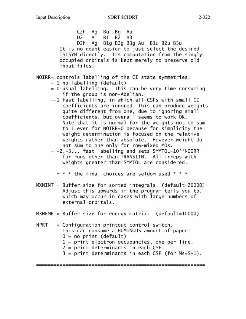
Input Description $DRT $CIDRT 2-322
C2h Ag Bu Bg Au D2 A B1 B2 B3 D2h Ag B1g B2g B3g Au B1u B2u B3u It is no doubt easier to just select the desired ISTSYM directly. Its computation from the singly occupied orbitals is kept merely to preserve old input files.
NOIRR= controls labelling of the CI state symmetries. = 1 no labelling (default) = 0 usual labelling. This can be very time consuming if the group is non-Abelian. =-1 fast labelling, in which all CSFs with small CI coefficients are ignored. This can produce weights quite different from one, due to ignoring small coefficients, but overall seems to work OK. Note that it is normal for the weights not to sum to 1 even for NOIRR=0 because for simplicity the weight determination is focused on the relative weights rather than absolute. However weight do not sum to one only for row-mixed MOs. = -2,-3... fast labelling and sets SYMTOL=10**NOIRR for runs other than TRANSITN. All irreps with weights greater than SYMTOL are considered.
* * * the final choices are seldom used * * *
MXNINT = Buffer size for sorted integrals. (default=20000) Adjust this upwards if the program tells you to, which may occur in cases with large numbers of external orbitals.
MXNEME = Buffer size for energy matrix. (default=10000)
NPRT = Configuration printout control switch. This can consume a HUMUNGUS amount of paper! 0 = no print (default) 1 = print electron occupancies, one per line. 2 = print determinants in each CSF. 3 = print determinants in each CSF (for Ms=S-1).
==========================================================

Input Description $MCSCF 2-323
==========================================================
$MCSCF group (for SCFTYP=MCSCF)
This group controls the MCSCF orbital optimizationstep. The difference between the five convergence methodsis outlined in the Further Information chapter, which youshould carefully study before trying MCSCF computations.
--- the next chooses the configuration basis ---
CISTEP = ALDET chooses the Ames Lab. determinant full CI, and requires $DET input. (default) = ORMAS chooses an Occupation Restricted Multiple Active Space determinant CI, requiring both $DET and $ORMAS inputs. = GUGA chooses the graphical unitary group CSFs, and requires $DRT input. This is the only value usable with the QUAD converger. = GENCI chooses the Ames Laboratory general CI, and requires $GEN input. = GMCCI chooses the Kyushu University general CI, and requires $GMCPT input.
--- the next five choose the orbital optimizer ---
FOCAS = a flag to select a method with a first order convergence rate. (default=.FALSE.) Parallel runs with FOCAS do not use MEMDDI.
SOSCF = a flag selecting an approximately second order convergence method, using an approximate orbital hessian. (default=.TRUE.) Parallel runs with SOSCF do not use MEMDDI.
FULLNR = a flag selecting a second order method, with an exact orbital hessian. (default=.FALSE.) Parallel runs with FULLNR require input of MEMDDI.
QUAD = a flag to pick a fully quadratic (orbital and CI coefficient) optimization method, which is applicable to FORS or non-FORS wavefunctions. QUAD may not be used with state-averaging. (default = .FALSE.) This converger can be used only in serial runs.
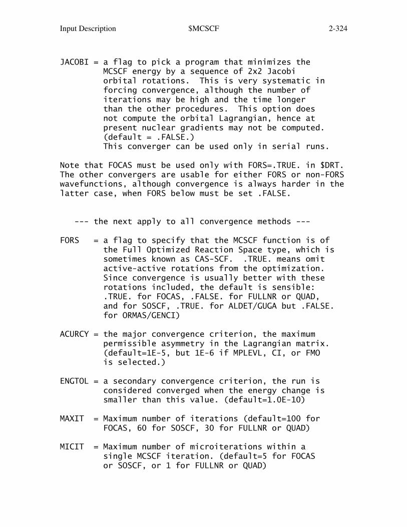
Input Description $MCSCF 2-324
JACOBI = a flag to pick a program that minimizes the MCSCF energy by a sequence of 2x2 Jacobi orbital rotations. This is very systematic in forcing convergence, although the number of iterations may be high and the time longer than the other procedures. This option does not compute the orbital Lagrangian, hence at present nuclear gradients may not be computed. (default = .FALSE.) This converger can be used only in serial runs.
Note that FOCAS must be used only with FORS=.TRUE. in $DRT.The other convergers are usable for either FORS or non-FORSwavefunctions, although convergence is always harder in thelatter case, when FORS below must be set .FALSE.
--- the next apply to all convergence methods ---
FORS = a flag to specify that the MCSCF function is of the Full Optimized Reaction Space type, which is sometimes known as CAS-SCF. .TRUE. means omit active-active rotations from the optimization. Since convergence is usually better with these rotations included, the default is sensible: .TRUE. for FOCAS, .FALSE. for FULLNR or QUAD, and for SOSCF, .TRUE. for ALDET/GUGA but .FALSE. for ORMAS/GENCI)
ACURCY = the major convergence criterion, the maximum permissible asymmetry in the Lagrangian matrix. (default=1E-5, but 1E-6 if MPLEVL, CI, or FMO is selected.)
ENGTOL = a secondary convergence criterion, the run is considered converged when the energy change is smaller than this value. (default=1.0E-10)
MAXIT = Maximum number of iterations (default=100 for FOCAS, 60 for SOSCF, 30 for FULLNR or QUAD)
MICIT = Maximum number of microiterations within a single MCSCF iteration. (default=5 for FOCAS or SOSCF, or 1 for FULLNR or QUAD)

Input Description $MCSCF 2-325
NWORD = The maximum memory to be used, the default is to use all available memory. (default=0)
CANONC = a flag to cause formation of the closed shell Fock operator, and generation of canonical core orbitals. This will order the MCC core by their orbital energies. (default=.TRUE.)
EKT = a flag to cause generation of extended Koopmans' theorem orbitals and energies. (Default=.FALSE.) For this option, see R.C.Morrison and G.Liu, J.Comput.Chem., 13, 1004-1010 (1992). Note that the process generates non-orthogonal orbitals, as well as physically unrealistic energies for the weakly occupied MCSCF orbitals. The method is meant to produce a good value for the first I.P.
NPUNCH = MCSCF punch option (analogous to $SCF NPUNCH) 0 do not punch out the final orbitals 1 punch out the occupied orbitals 2 punch out occupied and virtual orbitals The default is NPUNCH = 2.
NPFLG = an array of debug print control. This is analagous to the same variable in $CIINP. Elements 1,2,3,4,6,8 make sense, the latter controls debugging the orbital optimization.
--- the next refers to SOSCF optimizations ---
NOFO = number of FOCAS iterations before switching to the SOSCF converger. May be 0, 1, ... (default=1). One FOCAS iteration at the first geometry permits a canonicalization of the virtual space to occur, which is likely to be crucial for convergence.
MCFMO = set to 1 to remove redandant orbital Lagrangian elements in FMO-MCSCF. Note that corresponding orbital rotations will still be optimised but not considered when deciding whether a run converged. This option is only in effect if detached bonds are present (for which redundant orbitals exist). Default: 1.
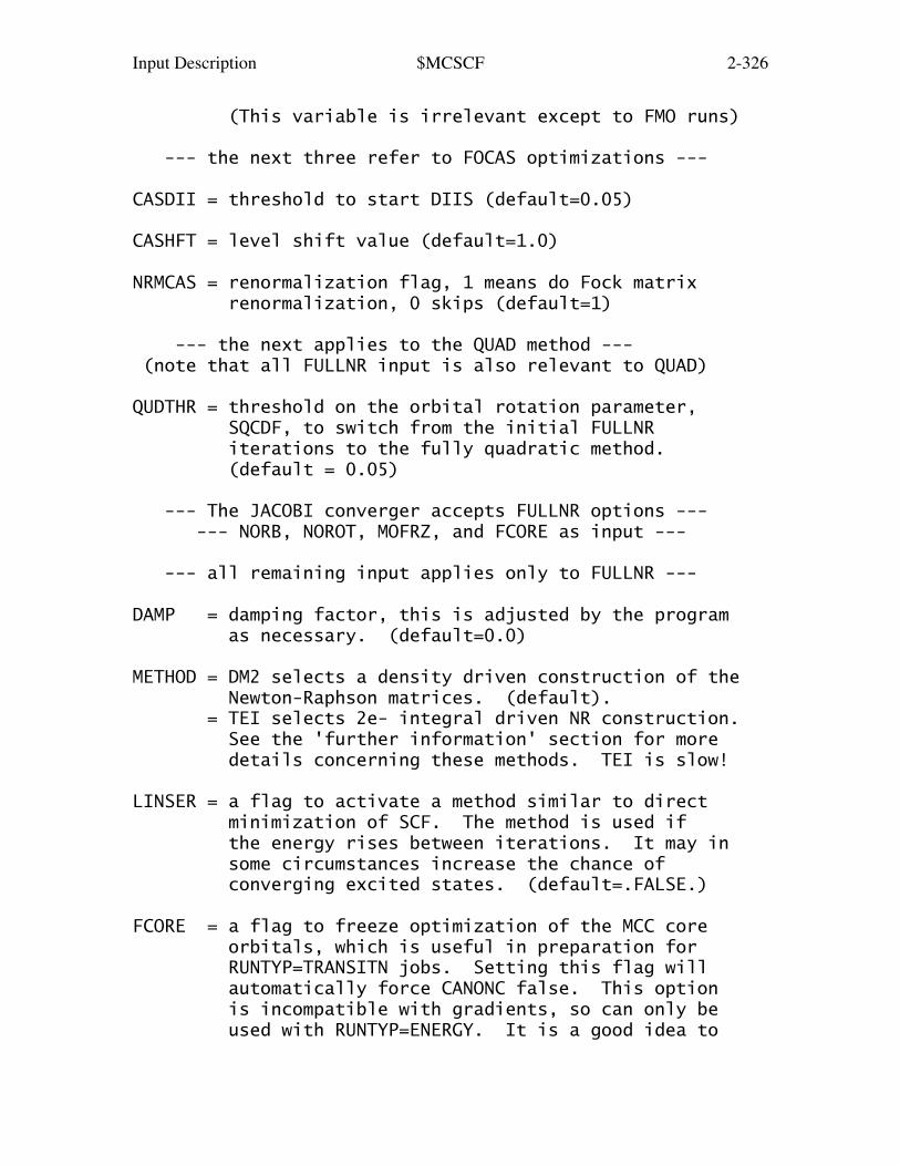
Input Description $MCSCF 2-326
(This variable is irrelevant except to FMO runs)
--- the next three refer to FOCAS optimizations ---
CASDII = threshold to start DIIS (default=0.05)
CASHFT = level shift value (default=1.0)
NRMCAS = renormalization flag, 1 means do Fock matrix renormalization, 0 skips (default=1)
--- the next applies to the QUAD method --- (note that all FULLNR input is also relevant to QUAD)
QUDTHR = threshold on the orbital rotation parameter, SQCDF, to switch from the initial FULLNR iterations to the fully quadratic method. (default = 0.05)
--- The JACOBI converger accepts FULLNR options --- --- NORB, NOROT, MOFRZ, and FCORE as input ---
--- all remaining input applies only to FULLNR ---
DAMP = damping factor, this is adjusted by the program as necessary. (default=0.0)
METHOD = DM2 selects a density driven construction of the Newton-Raphson matrices. (default). = TEI selects 2e- integral driven NR construction. See the 'further information' section for more details concerning these methods. TEI is slow!
LINSER = a flag to activate a method similar to direct minimization of SCF. The method is used if the energy rises between iterations. It may in some circumstances increase the chance of converging excited states. (default=.FALSE.)
FCORE = a flag to freeze optimization of the MCC core orbitals, which is useful in preparation for RUNTYP=TRANSITN jobs. Setting this flag will automatically force CANONC false. This option is incompatible with gradients, so can only be used with RUNTYP=ENERGY. It is a good idea to
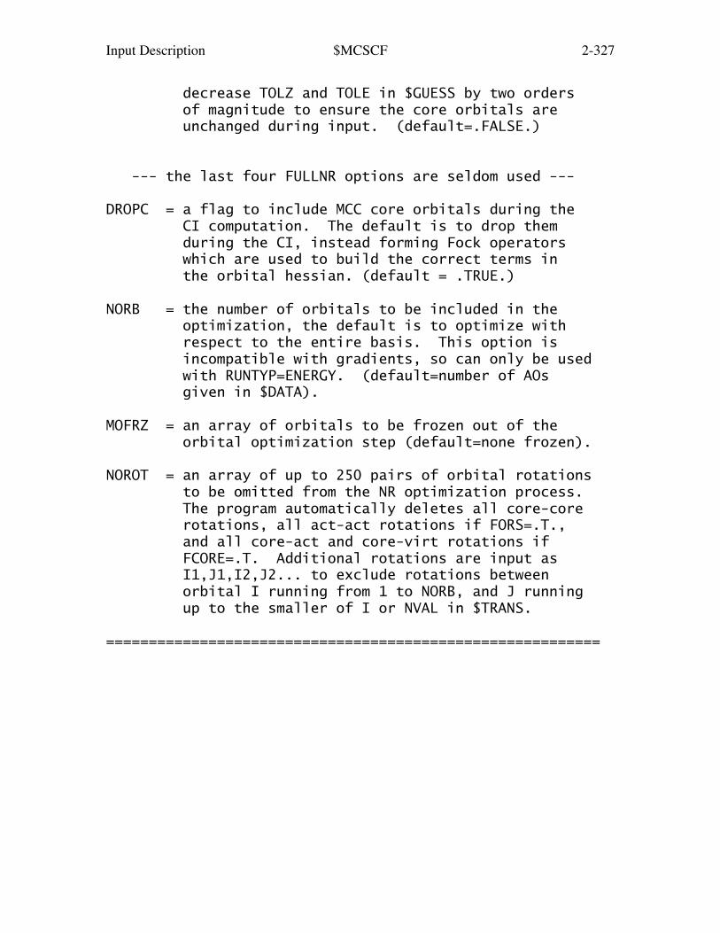
Input Description $MCSCF 2-327
decrease TOLZ and TOLE in $GUESS by two orders of magnitude to ensure the core orbitals are unchanged during input. (default=.FALSE.)
--- the last four FULLNR options are seldom used ---
DROPC = a flag to include MCC core orbitals during the CI computation. The default is to drop them during the CI, instead forming Fock operators which are used to build the correct terms in the orbital hessian. (default = .TRUE.)
NORB = the number of orbitals to be included in the optimization, the default is to optimize with respect to the entire basis. This option is incompatible with gradients, so can only be used with RUNTYP=ENERGY. (default=number of AOs given in $DATA).
MOFRZ = an array of orbitals to be frozen out of the orbital optimization step (default=none frozen).
NOROT = an array of up to 250 pairs of orbital rotations to be omitted from the NR optimization process. The program automatically deletes all core-core rotations, all act-act rotations if FORS=.T., and all core-act and core-virt rotations if FCORE=.T. Additional rotations are input as I1,J1,I2,J2... to exclude rotations between orbital I running from 1 to NORB, and J running up to the smaller of I or NVAL in $TRANS.
==========================================================
Input Description $MRMP 2-328
==========================================================
$MRMP group (relevant if SCFTYP=MCSCF, MPLEVL=2)
This group allows you to specify which multi-referenceperturbation program is executed. At the present time, thedeterminant and CSF programs produce identical results, sothe choice is largely one of computer efficiency.
MRPT = DETMRPT requests a determinant program. The MCSCF computation must use CISTEP=ALDET, as this program inherits orbital spaces, and state selection options only from a $DET group. See $DETPT for related input. (default for most runs) = MCQDPT requests a CSF (GUGA based) program. This is the only program that can do spin-orbit MRPT, apply energy denominators in case of so-called "intruder states", or find the weight of the MCQDPT zeroth order state. CISTEP can be ALDET or GUGA, your choice. See $MCQDPT for related input. (default for RUNTYP=TRANSITN) = GMCPT requests a determinant based program that can use non-CAS type reference functions, including ORMAS or user defined lists. See $GMCPT for related input.
Both the DETMRPT and MCQDPT programs produce numericallyidentical results, if you select a tight value ofTHRGEN=1D-12 for the latter program (in some cases you mayalso need to tighten the CI convergence criteria). Eightor more decimal place energy agreement between the twocodes has been observed, when being careful about thesecutoffs. This is true whether the codes are running insingle state mode, which the literature calls MRMP, or inmulti-state mode, which the literature calls MCQDPT.
Generally speaking, the determinant code uses direct CItechnology to avoid disk I/O, and is much faster when usedwith larger active spaces (particularly above 12 activeorbitals). The determinant code uses essentially no diskspace beyond that required by the MCSCF itself. Thedeterminant code uses native integral transformation codes,
Input Description $MRMP 2-329
including the distributed memory parallel transformation.However, the determinant code is perhaps a bit slower whenthere is a small active space and very many filled valenceorbitals included in the PT. Both codes exploitdistributed memory parallelization.
The determinant program is relatively new, and still lackscomplete control of state weights and canonicalization. Becareful to read in only canonicalized core, active, andvirtual MOs if you pick RDVECS=.TRUE. with this program.If you have any doubts about transitioning to thedeterminant code, please try running a calculation bothways, checking that you get the same results.
Please note that the CASPT2 equations are not implementedin GAMESS, and thus your runs should be described as beingMRMP/MCQDPT in any publications. See REFS.DOC for moredetails about different multireference PTs.
RDVECS = a flag controlling whether the orbitals should be MCSCF optimized in this run. A value of .TRUE. means that your converged MCSCF orbitals are being given in $VEC, and the program will branch to the perturbation treatement. (default=.FALSE.)
notes:If you select RDVECS, and are not doing spin-orbit couplingwith the CSF program, $GUESS method GUESS=MOREAD is used toprocess the orbitals. Its options such as NORB and PURIFYwill apply to reading the $VEC group, and as always, MOREADin $GUESS will orthogonalize.If you are the CSF program for spin-orbit coupling, $GUESSis ignored, and the $VEC or $VECn group must contain allvirtuals. The orbitals will not be reorthogonalized unlessyou select the MODVEC option.
In either case, if your orbitals are not orthogonal, youare better off repeating MCSCF with RDVECS=.FALSE.!
MODVEC = 0 skip orthogonalization (default) = 1 do orthogonalization in the SO-MCQDPT program.
==========================================================
Input Description $DETPT 2-330
==========================================================
$DETPT group (relevant if SCFTYP=MCSCF and MPLEVL=2)
This input group applies to the determinant-basedmulti-reference perturbation theory program, if chosen byMRPT=DETMRPT in $MRMP group.
When applied to only one state, the theory is known asmulti-reference Moller-Plesset (MRMP), but the term MCQDPTis used when this theory is used in its multi-state form.Please note that this perturbation theory is not the samething as the CASPT2 theory, and should -NEVER- be calledthat. A more complete discussion may be found in the'Further Information' chapter.
NVAL = number of filled valence orbitals in the MCSCF to be included in the dynamic correlation treatment. This is analogous to NMODOC in the $MCQDPT group. The number of frozen cores orbitals is found by subtracting NVAL from NCORE in $DET, so that you need not specify the chemical core's size. Also, there is no input for specifying the active space, which is inherited from $DET. The default for NVAL correlates valence orbitals, but freezes any chemical cores.
NEXT = number of external orbitals to use. The default means to use all of them (default=-1).
NOS = a flag to use MCSCF natural orbitals rather than canonicalized orbitals as the basis of the PT. This changes the numerical results!!!
Omitting NPTST, IPTST, and WPTST is the simplest option,meaning that any state with a non-zero WSTATE in $DET isincluded in the pertubation. Canonicalization of theorbitals is normally done by the MCSCF program, see CANONCin $MCSCF. However, if not, or if the state weights arechanged, the canonicalization is done in the perturbationcode, according to CANON in this group. The default is themost computationally efficient.
CANON = flag to request canonicalization. Default=.TRUE.

Input Description $DETPT 2-331
Turning off canonicalization is for experimental purposes, so most runs should not avoid it. The canonicalization will be done in the perturbation code under three circumstances, RDVECS=.TRUE. was used, at the first geometry, the MCSCF step skipped canonicalization, or you enter NPTST/IPTST/SPTST information. Canonicalization uses the state averaged density matrix to build the "standard Fock operator", and involves diagonalizing its diagonal sub-blocks.
NPTST = the number of states to include in generation of the unperturbed CAS states. If NPTST is chosen, spins of the states will be ignored, like using PURES=.F. in $DET, so you must be careful in your matching IPTST input.
IPTST = an array of CAS-CI states to be included in the perturbation theory, give NPTST values.
WPTST = an array of state weights. Like NPTST/IPTST, the default for WPTST is derived from WSTATE in $DET.
example: NPTST=3 IPTST(1)=1,3,5 might be used to includethree singlets, S0,S1,S2 in a MCQDPT-type treatment, butskip over T1 and T2. You will have done an earlier CI orMCSCF run, in order to know that you need NPTST five orhigher to capture the lowest three singlets, and that thesesinglets appear where they do. NSTATE in $DET must be atleast 5 in this example, to find enough roots.
==========================================================
Input Description $MCQDPT 2-332
==========================================================
$MCQDPT group (relevant if SCFTYP=MCSCF and MPLEVL=2)
Controls 2nd order MCQDPT (multiconfiguration quasi-degenerate perturbation theory) runs, if requested byMPLEVL=2 in $CONTRL. MCQDPT2 is implemented only for FORS(aka CASSCF) wavefunctions. The MCQDPT method is amultistate, as well as multireference perturbation theory.The implementation is a separate program, interfaced toGAMESS, with its own procedures for determination of thecanonical MOs, CSF generation, integral transformation, CIin the reference CAS, etc. Therefore some of the input inthis group repeats data given elsewhere, particularly for$DET/$DRT.
Analytic gradients are not available. Spin-orbitcoupling may be treated as a perturbation, included at thesame time as the energy perturbation. If spin-orbitcalculations are performed, the input groups for eachmultiplicity are named $MCQD1, $MCQD2, ... rather than$MCQDPT. Parallel calculation is enabled.
When applied to only one state, the theory is known asmulti-reference Moller-Plesset (MRMP), but the term MCQDPTis used when this theory is used in its multi-state form.Please note that this perturbation theory is not the samething as the CASPT2 theory, and should -NEVER- be calledthat. A more complete discussion may be found in the'Further Information' chapter.
*** MCSCF reference wavefunction ***
NEL = total number of electrons, including core. (default from $DATA and ICHARG in $CONTRL)
MULT = spin multiplicity (default from $CONTRL)
NMOACT = Number of orbitals in FORS active space (default is the active space in $DET or $DRT)NMOFZC = number of frozen core orbitals, NOT correlated in the perturbation calculation. (default is number of chemical cores)NMODOC = number of orbitals which are doubly occupied in every MCSCF configuration, that is, not active
Input Description $MCQDPT 2-333
orbitals, which are to be included in the perturbation calculation. (The default is all valence orbitals between the chemical core and the active space)NMOFZV = number of frozen virtuals, NOT occupied during the perturbation calculation. The default is to use all virtuals in the MP2. (default=0)
If the input file does not provide a $DET or $DRT, the usermust give NMOFZC, NMODOC, and NMOACT correctly here.
ISTSYM = the state symmetry of the target state(s). This is given as an integer, note that only Abelian groups in $DATA are supported: ISTSYM= 1 2 3 4 5 6 7 8 C1 A Ci Ag Au Cs A' A'' C2 A B C2v A1 A2 B1 B2 C2h Ag Bu Bg Au D2 A B1 B2 B3 D2h Ag B1g B2g B3g Au B1u B2u B3u (The default is inherited from $DET or $DRT)
NOSYM = 0 use CSF symmetry (see the ISTSYM keyword). off diagonal perturbations vanish if states are of different symmetry, so the most efficient computation is a separate run for every space symmetry. (default) 1 turn off CSF state symmetry so that all states are treated at once. ISTSYM is ignored. Presently this option does not seem to work!! -1 Symmetry purify the orbitals. Since $GUESS is not read by MCQDPT runs, this option can be used as a substitute for its PURIFY. After cleaning the orbitals, they are reorthogonalised within each irrep and within each group (core, double, active, virtual) separately. Since this occurs without MCSCF optimization if you have chosen to use RDVECS in $MRMP, it is *your* responsibility to ensure that any purification of the orbitals is small enough that the CAS energies for the original CASSCF and the CAS-CI performed during the MCQDPT are the same!
Input Description $MCQDPT 2-334
*** perturbation specification ***
KSTATE= state is used (1) or not (0) in the MCQDPT2. Maximum of 20 elements, including zeros. For example, if you want the perturbation correction to the second and the fourth roots, KSTATE(1)=0,1,0,1 See also WSTATE. (default=1,0,0,0,0,0,0,...)
*** Intruder State Removal ***
EDSHFT = energy denominator shifts. (default=0.0,0.0) See also REFWGT.
Intruder State Avoidance (ISA) calculations can be made bychanging the energy denominators around poles (where thedenominator is zero). Each denominator x is replaced by x+ EDSHFT/x, so that far from the poles (when x is large)the effect of such change is small. EDSHFT is an array oftwo values, the first is used in spin-free MCQDPT, and thesecond is for spin-orbit MCQDPT. Both values are used ifRUNTYP=TRNSTN, only the first is used otherwise. Asuggested pair of values is 0.02,0.1, but experimentationwith your system is recommended. Setting these values tozero is ordinary MCQDPT, whereas infinite collapses to theMCSCF reference.
Note that the energy denominators (which are ket-dependentin MCQDPT) are changed in a different way for each ket-vector, that is, for each row in MCQDPT Hamiltonian matrix.In other words, the zeroth order energies are not"universal", but state specific. This is strictly speakingan inconsistency in defining zeroth order energies that areusually chosen "universally".
In order to maintain continuity when studying a PES, oneusually uses the same EDSHFT values for all points on PES.In order to study the potential surface for any extendedrange of geometries, it is recommended to use ISA, as it isquite likely that one or more regions of the PES will beunphysical due to intruder states.
For an example of how intruder states can appear at somepoints on the PES, see Figures 1,2,7 of

Input Description $MCQDPT 2-335
K.R.Glaesemann, M.S.Gordon, H.Nakano Phys.Chem.Chem.Phys. 1, 967-975(1999)and also H.A.Witek, D.G.Fedorov, K.Hirao, A.Viel, P.-O.Widmark J.Chem.Phys. 116, 8396-406(2002)For a discussion of intruder state removal from MCQDPT, see H.A.Witek, Y.-K.Choe, J.P.Finley, K.Hirao J.Comput.Chem. 23, 957-965(2002)
REFWGT = a flag to request decomposition of the second order energy into internal, semi-internal, and external contributions, and to obtain the weight of the MCSCF reference in the 1st order wave function. This option significantly increases the run time! When you run in parallel, only the transformation steps will speed up, as the PT part of the reference weight calculation has not been adapted for speedups (default=.FALSE.)
The EDSHFT option does not apply if REFWGT is used. One purpose of using REFWGT is to try to understand the nature of the intruder states.
*** Canonical Fock orbitals ***
IFORB = 0 omit this step. = 1 determine the canonical Fock orbitals. (default) = 3 canonicalise the Fock orbitals averaged over all $MCQDx input groups.
This option pertains only to RUNTYP=TRANSITN. It isprimarily meant to include spin-orbit coupling perturbationinto the energy perturbation, but could also be used inconjunction with OPERAT=DM to calculate only the secondorder energy perturbation. IFORB=3 means that WSTATE isused as follows: In each $MCQDx group, the WSTATE weightsare divided by the total number of states (sum(i)IROOTS(i)), so the sum over all WSTATE values in all $MCQDxgroups is normalized to sum to 1. Thus there is nonormalization to 1 within each $MCQDx group.This option might be used to speed up an atomic MCQDPT,e.g. if computing the 3-P ground state of carbon, one wouldwant to average over all three spatial components of the Pterm, to be sure of spatial degeneracy, but then run theperturbation using symmetry, separately on the B1g+B2g+B3g

Input Description $MCQDPT 2-336
subspecies (within D2h) of a P term. It is very importantto give weights appropriate for the symmetry, the inputrequires care.
WSTATE = weight of each CAS-CI state in computing the closed shell Fock matrix. You must enter 0.0 whenever the same element in KSTATE is 0. In most cases setting the WSTATEs for states to be included in the MCQDPT to equal weights is the best, and this is the default.
*** Miscellaneous options ***
ISELCT is an option to select only the important CSFs for inclusion into the CAS-CI reference states. Set to 1 to select, or 0 to avoid selection of CSFs (default = 0) All CSFs in a preliminary complete active space CI whose CI coefficients exceed the square root of THRWGT are kept in a smaller CI to determine the zero-th order states. Note that the CSFs with smaller coefficients, while excluded from the reference states, are still used during the perturbation calculation, so most of their energy contribution is still retained. This can save appreciable computer time in cases with large active spaces.
THRWGT = weight threshold for retaining CSFs in selected configuration runs. In quantum mechanics, the weight of a CSF is the square of its CI coefficient. (default=1d-6)
THRGEN = threshold for one-, two-, and three-body density matrix elements in the perturbation calculation. The default gives about 5 decimal place accuracy in energies. Increase to 1.0D-12 if you wish to obtain higher accuracy, for example, in numerical gradients (default=1D-8). Tightening THRGRN and perhaps CI diagonalization should allow 7-8 decimal place agreement with the determinant code.
THRENE = threshold for the energy convergence in the
Input Description $MCQDPT 2-337
Davidson's method CAS-CI. (default=-1.0D+00)
THRCON = threshold for the vector convergence in the Davidson's method CAS-CI. (default=1.0D-06)
MDI = dimension of small Hamiltonian diagonalized to prepare initial guess CI states. (default=50)
MXBASE = maximum number of expansion vectors in the Davidson diagonalization subspace (e.g. MXXPAN). (default=50)
NSOLUT = number of states to be solved for in the Davidson's method, this might need to exceed the number of states in the perturbation treatment in order to "capture" the correct roots.
NSTOP = maximum number of iterations to permit in the Davidson's diagonalization.
LPOUT = print option, 0 gives normal printout, while <0 gives debug print (e.g. -1, -5, -10, -100) In particular, LPOUT=-1 gives more detailed timing information. (default=0)
The next three parameters refer to parallel execution:
DOORD0 = a flag to select reordering of AO integrals which speeds the integral transformations. This reduces disk writes, but increases disk reads, so you can try turning it off if your machine has slow writes. (default=.TRUE.)
PARAIO = access 2e- integral file on every node, at the same time. This affects only runs with DOORD0 true, and it may be useful to turn this off in the case of SMP nodes sharing a common disk drive. (default=.TRUE.)
DELSCR = a flag to delete file 56 containing half- transformed integrals after it has been used. This reduces total disk requirements if this file is big. (default=.FALSE.)
Input Description $MCQDPT 2-338
Note that parallel execution will be more effective if youuse distributed memory, MEMDDI in $SYSTEM. UsingAOINTS=DIST in $TRANS is likely to be helpful in situationswith relatively poor I/O rates compared to communication,e.g. SMP enclosures forced to share a single scratch disksystem. See PROG.DOC for more information on parallelexecution.
Finally, there are additional very specialized options,described in the source code routine MQREAD: IROT, LENGTH,MAXCSF, MAXERI, MAXROW, MXTRFR, THRERI, MAINCS, NSTATE
==========================================================

Input Description $CASCI 2-339
==========================================================
$CASCI group (relevant to SCFTYP=RHF MPLEVL=2)
This group carries out the Improved Virtual Orbital -Complete Active Space CI method of Freed, Chaudhuri, andco-workers. IVO-CASCI starts with a RHF reference, andthen generates IVOs, which are used in a CI computationwithin an active space chosen by the user. The inputconsists of this group, the $MCQDPT group, and perhaps a$IVOORB group, along with SCFTYP=RHF and MPLEVL=2. MULT in$CONTRL applies to the SCF reference, while MULT in $MCQDPTselects the spin of the IVO-CASCI state(s). Doublets aretreated by using a cation RHF reference.
IVOCAS = a flag to turn on IVO-CASCI computation. This is usually the only input required (default=.FALSE.)
MOLIST = a flag to request complete control over the active space specification. The default uses the parameters in $MCQDPT to select from the IVOs with the lowest energy. (default=.FALSE.)
DEGENR = a flag to indicate the HOMO is degenerate. The program should set this for you.
PRINT = a flag to print debugging info (default=.FALSE.)
The user should request IFORB=0 in $MCQDPT to suppress itsgeneration of canonical orbitals, so that the IVOs areused. A Huckel guess is usually fine. The $MCQDPT shoulddefine the active orbitals taken from the IVO set by givingNMOFZC, NMODOC, and NMOACT, and the electronic state isspecified by that group's MULT, NSTATE, and NSTSYM.
References:
D.M.Potts, C.M.Taylor, R.K.Chaudhuri, K.F.Freed J.Chem.Phys. 114, 2592-2600(2001)R.K.Chaudhuri, K.F.Freed, S.A.Abrash, D.M.Potts J.Mol.Spectrosc. 547, 83-96(2001)R.K.Chaudhuri, K.F.Freed J.Chem.Phys. 126, 114103/1-6(2007)
A simple example follows,
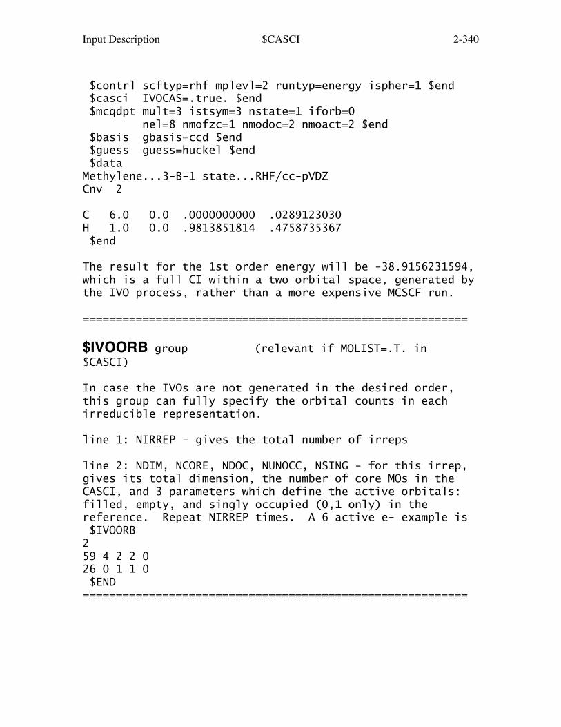
Input Description $CASCI 2-340
$contrl scftyp=rhf mplevl=2 runtyp=energy ispher=1 $end $casci IVOCAS=.true. $end $mcqdpt mult=3 istsym=3 nstate=1 iforb=0 nel=8 nmofzc=1 nmodoc=2 nmoact=2 $end $basis gbasis=ccd $end $guess guess=huckel $end $dataMethylene...3-B-1 state...RHF/cc-pVDZCnv 2
C 6.0 0.0 .0000000000 .0289123030H 1.0 0.0 .9813851814 .4758735367 $end
The result for the 1st order energy will be -38.9156231594,which is a full CI within a two orbital space, generated bythe IVO process, rather than a more expensive MCSCF run.
==========================================================
$IVOORB group (relevant if MOLIST=.T. in$CASCI)
In case the IVOs are not generated in the desired order,this group can fully specify the orbital counts in eachirreducible representation.
line 1: NIRREP - gives the total number of irreps
line 2: NDIM, NCORE, NDOC, NUNOCC, NSING - for this irrep,gives its total dimension, the number of core MOs in theCASCI, and 3 parameters which define the active orbitals:filled, empty, and singly occupied (0,1 only) in thereference. Repeat NIRREP times. A 6 active e- example is $IVOORB259 4 2 2 026 0 1 1 0 $END==========================================================

Input Description $CISORT $GUGEM 2-341
The input groups $CISORT, $GUGEM, $GUGDIA, $GUGDM, $GUGDM2,$LAGRAN, and $TRFDM2 pertain only to GUGA CI, chosen byeither CITYP=GUGA or CISTEP=GUGA. The most important ofthese values may be given for determinant runs (using thesame keyword spellings) in the $DET group.
==========================================================
$CISORT group (relevant for GUGA -CI- or -MCSCF-) This group provides further control over the sortingof the transformed molecular integrals into the order theGUGA program requires.
NDAR = Number of direct access records. (default = 2000)
LDAR = Length of direct access record (site dependent)
NBOXMX = Maximum number of boxes in the sort. (default = 200)
NWORD = Number of words of fast memory to use in this step. A value of 0 results in automatic use of all available memory. (default = 0)
NOMEM = 0 (set to one to force out of memory algorithm)
==========================================================
$GUGEM group (relevant for GUGA -CI- or -MCSCF-)
This group provides further control over thecalculation of the energy (Hamiltonian) matrix.
CUTOFF = Cutoff criterion for the energy matrix. (default=1.0E-8)
NWORD = not used.
==========================================================
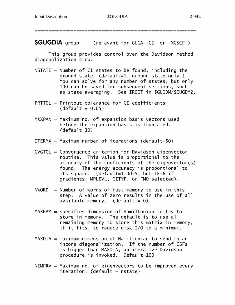
Input Description $GUGDIA 2-342
==========================================================
$GUGDIA group (relevant for GUGA -CI- or -MCSCF-)
This group provides control over the Davidson methoddiagonalization step.
NSTATE = Number of CI states to be found, including the ground state. (default=1, ground state only.) You can solve for any number of states, but only 100 can be saved for subsequent sections, such as state averaging. See IROOT in $GUGDM/$GUGDM2.
PRTTOL = Printout tolerance for CI coefficients (default = 0.05)
MXXPAN = Maximum no. of expansion basis vectors used before the expansion basis is truncated. (default=30)
ITERMX = Maximum number of iterations (default=50)
CVGTOL = Convergence criterion for Davidson eigenvector routine. This value is proportional to the accuracy of the coeficients of the eigenvector(s) found. The energy accuracy is proportional to its square. (default=1.0d-5, but 1E-6 if gradients, MPLEVL, CITYP, or FMO selected).
NWORD = Number of words of fast memory to use in this step. A value of zero results in the use of all available memory. (default = 0)
MAXHAM = specifies dimension of Hamiltonian to try to store in memory. The default is to use all remaining memory to store this matrix in memory, if it fits, to reduce disk I/O to a minimum.
MAXDIA = maximum dimension of Hamiltonian to send to an incore diagonalization. If the number of CSFs is bigger than MAXDIA, an iterative Davidson procedure is invoked. Default=100
NIMPRV = Maximum no. of eigenvectors to be improved every iteration. (default = nstate)
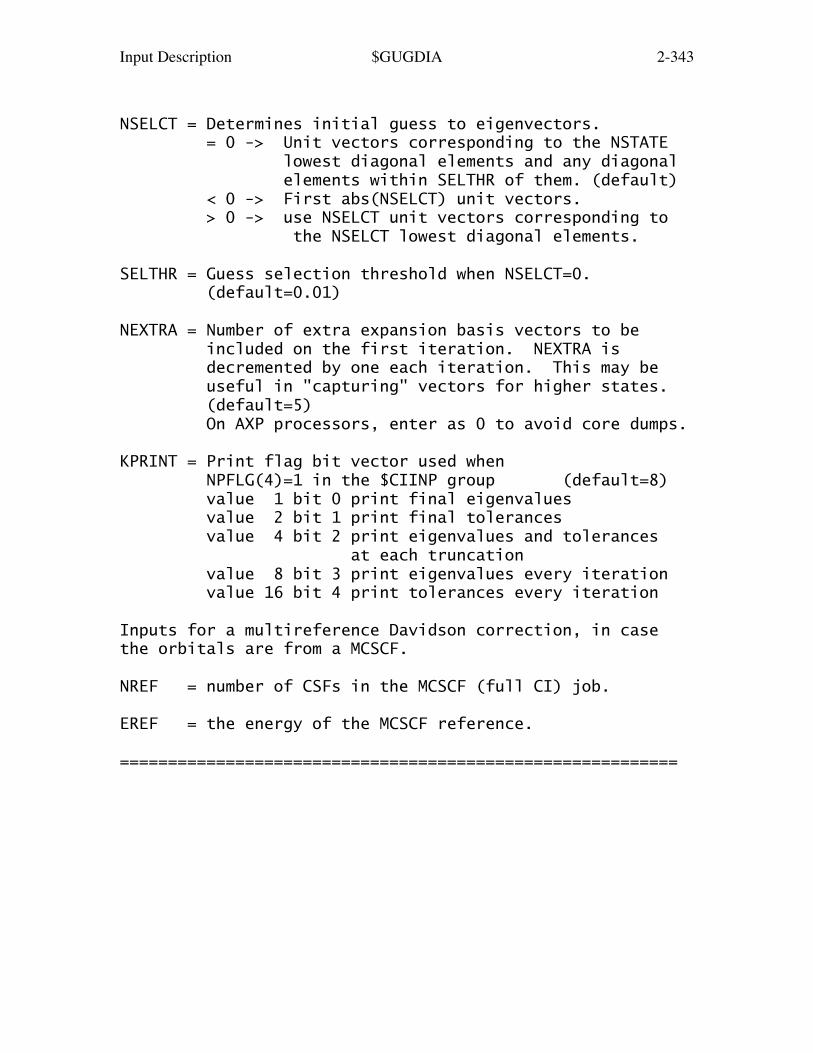
Input Description $GUGDIA 2-343
NSELCT = Determines initial guess to eigenvectors. = 0 -> Unit vectors corresponding to the NSTATE lowest diagonal elements and any diagonal elements within SELTHR of them. (default) < 0 -> First abs(NSELCT) unit vectors. > 0 -> use NSELCT unit vectors corresponding to the NSELCT lowest diagonal elements.
SELTHR = Guess selection threshold when NSELCT=0. (default=0.01)
NEXTRA = Number of extra expansion basis vectors to be included on the first iteration. NEXTRA is decremented by one each iteration. This may be useful in "capturing" vectors for higher states. (default=5) On AXP processors, enter as 0 to avoid core dumps.
KPRINT = Print flag bit vector used when NPFLG(4)=1 in the $CIINP group (default=8) value 1 bit 0 print final eigenvalues value 2 bit 1 print final tolerances value 4 bit 2 print eigenvalues and tolerances at each truncation value 8 bit 3 print eigenvalues every iteration value 16 bit 4 print tolerances every iteration
Inputs for a multireference Davidson correction, in casethe orbitals are from a MCSCF.
NREF = number of CSFs in the MCSCF (full CI) job.
EREF = the energy of the MCSCF reference.
==========================================================

Input Description $GUGDM 2-344
==========================================================
$GUGDM group (relevant for GUGA -CI-)
This group provides further control over formation ofthe one electron density matrix. See NSTATE in $GUGDIA.
NFLGDM = Array controlling each state's density formation. 0 -> do not form density for this state. 1 -> form density and natural orbitals for this state, print and punch occ.nums. and NOs. 2 -> same as 1, plus print density over MOs. The default is NFLGDM(1)=1,0,0,...,0 meaning only ground state NOs are generated.Note that forming the 1-particle density for a state isnegligible compared to diagonalization time for that state.
IROOT = The root whose density matrix is saved on desk for later computation of properties. You may save only one state's density per run. By default, this is the ground state (default=1).
WSTATE = An array of up to 100 weights to be given to the 1 body density of each state. The averaged density will be used for property computations, as well as "state averaged natural orbitals". The default is to use NFLGDM/IROOT, unless WSTATE is given, when NFLGDM/IROOT are ignored. It is not physically reasonable to average over any CI states that are not degenerate, but it may be useful to use WSTATE to produce a totally symmetric density when the states are degenerate.
IBLOCK = Density blocking switch. If nonzero, the off diagonal block of the density above row IBLOCK will be set to zero before the (now approximate) natural orbitals are found. One use for this is to keep the internal and external orbitals in a FOCI or SOCI calculation from mixing, where IBLOCK is the highest internal orbital. (default=0)
NWORD = Number of words of memory to use. Zero means use all available memory (default=0).
==========================================================
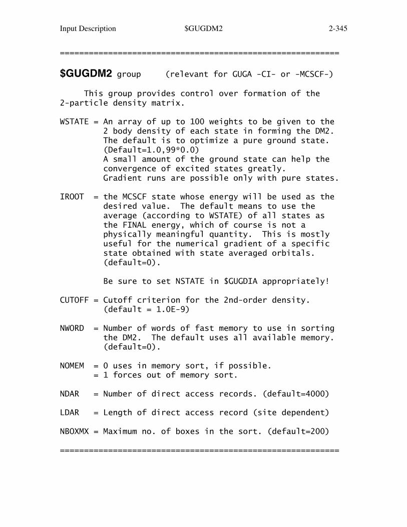
Input Description $GUGDM2 2-345
==========================================================
$GUGDM2 group (relevant for GUGA -CI- or -MCSCF-)
This group provides control over formation of the2-particle density matrix.
WSTATE = An array of up to 100 weights to be given to the 2 body density of each state in forming the DM2. The default is to optimize a pure ground state. (Default=1.0,99*0.0) A small amount of the ground state can help the convergence of excited states greatly. Gradient runs are possible only with pure states.
IROOT = the MCSCF state whose energy will be used as the desired value. The default means to use the average (according to WSTATE) of all states as the FINAL energy, which of course is not a physically meaningful quantity. This is mostly useful for the numerical gradient of a specific state obtained with state averaged orbitals. (default=0).
Be sure to set NSTATE in $GUGDIA appropriately!
CUTOFF = Cutoff criterion for the 2nd-order density. (default = 1.0E-9)
NWORD = Number of words of fast memory to use in sorting the DM2. The default uses all available memory. (default=0).
NOMEM = 0 uses in memory sort, if possible. = 1 forces out of memory sort.
NDAR = Number of direct access records. (default=4000)
LDAR = Length of direct access record (site dependent)
NBOXMX = Maximum no. of boxes in the sort. (default=200)
==========================================================

Input Description $LAGRAN 2-346
==========================================================
$LAGRAN group (relevant for GUGA -CI- gradient)
This group provides further control over formation ofthe CI Lagrangian, a quantity which is necessary for thecomputation of CI gradients.
NOMEM = 0 form in core, if possible = 1 forces out of core formation
NWORD = 0 (0=use all available memory)
NDAR = 4000
LDAR = Length of each direct access record (default is NINTMX from $INTGRL)
==========================================================
Input Description $TRFDM2 2-347
==========================================================
$TRFDM2 group (relevant for GUGA -CI- gradient)
This group provides further control over the backtransformation of the 2 body density to the AO basis.
NOMEM = 0 transform and sort in core, if possible = 1 transform in core, sort out of core, if poss. = 2 transform out of core, sort out of core
NWORD = 0 (0=use all available memory)
CUTOFF= 1.0D-9, threshold for saving DM2 values
NDAR = 2000
LDAR = Length of each direct access record (default is system dependent)
NBOXMX= 200
==========================================================
Usually neither $LAGRAN or $TRFDM2 group are given. Sincethese groups are normally used only for CI gradient runs,we list here the restrictions on the GUGA CI gradients: a) SCFTYP=RHF, only b) no FZV orbitals in $CIDRT, all MOs must be used. c) the derivative integrals are computed in the 2nd derivative code, which is limited to spd basis sets. d) the code does not run in parallel. e) Use WSTATE in $GUGDM2 to specify the state whose gradient is to be found. Use IROOT in $GUGDM to specify the state whose other properties will be found. These must be the same state! f) excited states often have different symmetry than the ground state, so think about GROUP in $CIDRT. g) the gradient can probably be found for any CI for which you have sufficient disk to do the CI itself. Time is probably about 2/3 additional.
See also $CISGRD for CI singles gradients.
===========================================================
Input Description $TRANST 2-348
$TRANST group (relevant for RUNTYP=TRANSITN) (only for CITYP=GUGA or MPLEVL=2)
This group controls the evaluation of the radiativetransition moment, or spin orbit coupling (SOC). An SOCcalculation can be based on variational CI wavefunctions,using GUGA CSFs, or based on 2nd order perturbation theoryusing the MCQDPT multireference perturbation theory.These are termed SO-CI and SO-MCQDPT below. The orbitalsare typically obtained by MCSCF computations, and sincethe CI or MCQDPT wavefunctions are based on those MCSCFstates, the zero-th order states are referred to below asthe CAS-CI states. SOC jobs prepare a model Hamiltonianin the CAS-CI basis, and diagonalize it to produce spin-mixed states, which are linear combinations of the CAS-CIstates. If scalar relativistic corrections were includedin the underlying spin-free wavefunctions, it is possibleeither to include or to neglect similar corrections to thespin-orbit integrals, see keyword NESOC in $RELWFN.
An input file to perform SO-CI will contain SCFTYP=NONE CITYP=GUGA MPLEVL=0 RUNTYP=TRANSITNwhile a SO-MCQDPT calculation will have SCFTYP=NONE CITYP=NONE MPLEVL=2 RUNTYP=TRANSITNThe SOC job will compute a Hamiltonian matrix as the sumof spin-free terms and spin-orbit terms, H = H-sf + H-so.For SO-CI, the matrix H-sf is diagonal in the CAS-CI statebasis, with the LS-coupled CAS-CI energies as the diagonalelements, and H-so contains only off-diagonal couplingsbetween these LS states, H-sf = CAS-CI spin-free E H-so = CAS SOC Hamiltonian (e.g. HSO1, HSO2P, HSO2)For SO-MCQDPT, the additional input PARMP defines thesematrices differently. For PARMP=0, the spin-free termhas diagonal and off-diagonal MCQDPT perturbations: H-sf - CAS-CI spin-free E + 2nd order spin-free MCQDPT H-so - CAS SOC HamiltonianFor PARMP not equal to 0, the spin orbit operator is alsoincluded into the perturbing Hamiltonian of the MCQDPT: H-sf - CAS-CI spin-free E + 2nd order spin-free MCQDPT H-so - CAS SOC Hamiltonian + 2nd order SO-MCQDPT
Pure transition moment calculations (OPERAT=DM) arepresently limited to CI wavefunctions, so please use only
Input Description $TRANST 2-349
CITYP=GUGA MPLEVL=0. The transition moments computed bySO-MCQDPT runs (see TMOMNT flag) will form the transitiondensity for the CAS-CI zeroth order states rather than the1st order perturbed wavefunctions.
Please see REFS.DOC for additional information on whatis actually a fairly complex input file to prepare.
OPERAT selects the type of transition being computed. = DM calculates radiative transition moment between states of same spin, using the dipole moment operator. (default) = HSO1 one-electron Spin-Orbit Coupling (SOC) = HSO2P partial two electron and full 1e- SOC, namely core-active 2e- contributions are computed, but active-active 2e- terms are ignored. This generally captures >90% of the full HSO2 computation, but with spin-orbit matrix element time similar to the HSO1 calculation. = HSO2 one and two-electron SOC, this is the full Pauli-Breit operator. = HSO2FF one and two-electron SOC, the form factor method gives the same result as HSO2, but is more efficient in the case of small active spaces, small numbers of CAS-CI states, and large atomic basis sets. This final option applies only to SO-CI.
PARMP = controls inclusion of the SOC terms in SO-MCQDPT, for OPERAT=HSO1 (default=1) or for HSO2P/HSO2 (default=3) only. 0 - no SOC terms should be included in the MCQDPT corrections at 2nd order, but they will be included in the CAS states on which the MCQDPT (i.e. up to 1st order) 1 - include the 1e- SOC perturbation in MCQDPT -1 - defined under "3", read on... 3 - full 1-electron and partial 2-electron in the form of the mean field perturbation (this is very similar to HSO2P, but in the MCQDPT2 perturbation). Only doubly occupied orbitals (NMODOC) are used for the core 2e terms. If the option is set to -1, then all core orbitals (NMOFZC+NMODOC) are used. Neither

Input Description $TRANST 2-350
calculation includes extra diagrams including filled orbitals, so both are "partial".PARMP=3 (or -1) has almost no extra cost compared toPARMP=1, but can only be used with OPERAT=HSO2 or HSO2P.The options -1 and 3 are not rigorously justified, contraryto HOS2P for a SO-CI, as 2e integrals with 2 core indicesappear in the second order in two ways. There is a mean-field addition to 1e integrals, which is included when youchoose PARMP=3 or -1. But, there are separate terms fromadditional diagrams that are not implemented, so that thereis some imbalance in including the partial 2e correction.Nevetheless, it may be better to include such "partial"partial 2e contributions than not to. Note that at firstorder in the energy (the CAS-CI states) the N-electronterms are treated exactly as specified by OPERAT.
NFFBUF = sets buffer size for form factors in SO-MCQDPT. (applies only to OPERAT = HSO1, HSO2 or HSO2P). This is a very powerful option that speeds up SO-MCQDPT calculations by precomputing the total multiplicative factor in front of each diagram so that the latter is computed only once (this is in fact what happens in MCQDPT). It is not uncommon for this option to speed up calculations by a factor of 10. Since this option forces running the SO-CASCI part twice (due to the SO-MCQDPT Hamiltonian being non-Hermitian), it is possible that in rare cases NFFBUF=0 may perform similarly or better. The upper bound for NFFBUF is NACT**2, where NACT=NOCC-NFZC. Due to the sparseness of the coupling constants it is usually sufficient to set NFFBUF to 3*NACT. To use the older way of dynamically computing form factors and diagrams on the fly, set NFFBUF to 0. Default: 3*(NOCC-NFZC)
It is advisable to tighten up the convergence criteria inthe $MCQDx groups since SOC is a fairly small effect, andthe spin-free energies should be accurately computed, forexample THRCON=1e-8 THRGEN=1e-10.
PARMP has a rather different meaning for OPERAT=HSO2FF:It refers to the difference between ket and bra's Ms, -1 do matrix elements for ms=-1 only 0 do matrix elements for ms=0 only 1 do matrix elements for ms=1 only
Input Description $TRANST 2-351
-2 do matrix elements for all ms (0, 1, and -1), which is the default. -3 calculates form factors so they can be saved
* * * next defines the orbitals and wavefunctions * * *
NUMCI = For SO-CI, this parameter tells how many CI calculations to do, and therefore defines how many $DRTx groups will be read in. For SO-MCQDPT, this parameter tells how many MCQDPT calculations to do, and therefore defines how many $MCQDx groups will be read in. (default=1) IROOTS, IVEX, NSTATE, and ENGYST below will all have NUMCI values. NUMCI may not exceed 64.You may wish to define one $DRTx or $MCQDx group for eachspatial symmetry representation occuring within each spinmultiplicity, as the use of symmetry during these separatecalculations may make the entire job run much faster.
NUMVEC = the meaning is different depending on the run: a) spin-orbit CI (SO-CI), Gives the number of different MO sets. This can be either 1 or 2, but 2 can be chosen only for FORS/CASSCF or FCI wavefunctions. (default=1) If you set NUMVEC=2 and you use symmetry in any of the $DRTx groups, you may have to use ISTSYM in the $DRT groups since the order of orbitals from the corresponding orbital transformation is unpredictable. b) spin-orbit perturbation (SO-MCQDPT), The option to have different MOs for different states is not implemented, so your job will have only one $VEC1 group, and IVEX will not normally be input. The absolute value of NUMVEC should be be equal to the value of NUMCI above. If NUMVEC positive, the orbitals in the $VEC1 will be used exactly as given, whereas if NUMVEC is a negative number, the orbitals will be canonicalized according to IFORB in $MCQDx. Using NUMVEC=-NUMCI and IFORB=3 in all $MCQDx to canonicalize over all states is recommended.Note that $GUESS is not read by this RUNTYP! Orbitals mustbe in $VEC1 and possibly $VEC2 input groups.

Input Description $TRANST 2-352
NFZC = For SO-CI, this is equal to NFZC in each $DRTx group. When NUMVEC=2, this is also the number of identical core orbitals in the two vector sets. For SO-MCQDPT, this should be NMOFZC+NMODOC given in each of the $MCQDx groups. The default is the number of AOs given in $DATA, this is not very reasonable.
NOCC = the number of occupied orbitals. For SO-CI this should be NFZC+NDOC+NALP+NAOS+NBOS+NVAL, but add the external orbitals if the CAS-CI states are CI-SD or FOCI or SOCI type instead of CAS. For SO-MCQDPT enter NUMFZC+NUMDOC+NUMACT. The default is the number of AOs given in $DATA, which is not usually correct.
Note: IROOTS, NSTATE, ENGYST, IVEX contain NUMCI values.
IROOTS = array containing the number of CAS-CI states to be used from each CI or MCQDPT calculation. The default is 1 for every calculation, which is probably not a correct choice for OPERAT=DM runs, but is quite reasonable for the HSO operators. The total number of states included in the SOC Hamiltonian is the summation of the NUMCI values of IROOTS times the multiplicity of each CI or MCQDPT. See also ETOL/UPPREN.
NSTATE = array containing the number of CAS-CI states to be found by diagonalising the spin-free Hamiltonians. Of these, the first IROOTS(i) states will be used to find transition moments or SOC. Obviously, enter NSTATE(i) >= IROOTS(i). The default for NSTATE(i) is IROOTS(i), but might be bigger if you are curious about the additional energies, or to help the Davidson diagonalizer. NSTATE is ignored by SO-MCQDPT runs, and you must ensure that your IROOTS input corresponds to the KSTATE option in $MCQDx.
ETOL = energy tolerance for CI state elimination. This applies only to SO-CI and OPERAT=HSO1,2,2P. After each CI finds NSTATE(i) CI roots for each $DRTx, the number of states kept in the run is

Input Description $TRANST 2-353
normally IROOTS(i), but ETOL applies the further constraint that the states kept be within ETOL of the lowest energy found for any of the $DRTx. The default is 100.0 Hartree, so that IROOTS is the only limitation.
UPPREN = similar to ETOL, except it is an absolute energy, instead of an energy difference.
IVEX = Array of indices of $VECx groups to be used for each CI calculation. The default for NUMVEC=2 is IVEX(1)=1,2,1,1,1,1,1..., and of course for NUMVEC=1, it is IVEX(1)=1,1,1,1,1... This applies only to CITYP=GUGA jobs.
ENGYST = energy values to replace the spin-free energies. This parameter applies to SO-CI only. A possible use for this is to use first or second order CI energies (FOCI or SOCI in $DRT) on the diagonal of the Hamiltonian (obtained in some earlier runs) but to use only CAS wavefunctions to evaluate off diagonal HSO matrix elements. The CAS-CI is still conducted to get CI coefs, needed to evaluate the off diagonal elements. Enter MXRT*NUMCI values as a square array, by the usual FORTRAN convention (that is, MXRT roots of $DRT1, MXRT roots of $DRT2 etc), in hartrees, with zeros added to fill each column to MXRT values. MXRT is the maximum value in the IROOTS array. (the default is the computed CAS-CI energies) See B.Schimmelpfennig, L.Maron, U.Wahlgren, C.Teichteil, H.Fagerli, O.Gropen Chem.Phys.Lett. 286, 261-266(1998).
* * * the next pertain only to spin-orbit runs * * *
RSTATE = sets the zero energy level format: ndrt*1000+iroot for adiabatic state (root) 0000 sets zero energy to the lowest diabatic root default: 1001 (1st root in $DRT1 or $MCQD1)
ZEFTYP specifies effective nuclear charges to use. = TRUE uses true nuclear charge of each atom,
Input Description $TRANST 2-354
except protons are removed if an ECP basis is being used (default). = 3-21G selects values optimized for the 3-21G basis, but these are probably appropriate for any all electron basis set. Rare gases, transition metals, and Z>54 will use the true nuclear charges. = SBKJC selects a set obtained for the SBKJC ECP basis set, specifically. It may not be sensible to use these for other ECP sets. Rare gases, lanthanides, and Z>86 will use the true nuclear charges.
ZEFF = an array of effective nuclear charges, overriding the charges chosen in ZEFTYP.
Note that effective nuclear charges can be used for any HSO type OPERAT, but traditionally these are used mainly for HSO1 as an empirical correction to the omission of the 2e- term, or to compensate for missing core orbitals in ECP runs.
ONECNT = uses a one-center approximation for SOC integrals: = 0 compute all SOC integrals without approximations = 1 compute only one-center 1e and 2e SOC integrals = 2 compute all 1e, but only one-center 2e integrals Numerical tests indicate the error of the one-center approximation (ONECNT=1) is usually on the order of a few wavenumbers for Li-Ne (a bit larger for F) and its errors appear to become negligible for anything heavier than Ne. ONECNT=1 appears to give a better balanced description than ONECNT=2. Very careful users can check how well the approximation works for their particular system by using ONECNT=0, then ONECNT=1, to compare the results. One important advantage of ONECNT=1/2 is that this removes the dependence of SOC 2e integrals upon the molecular geometry. This means the program needs to compute SOC 2e integrals only once for a given set of atoms and then they can be read by using SOC integral restart. RUNTYP=SURFACE automatically takes advantage of this fact.
JZ controls the calculation of Jz eigenvalues = 0 do not perform the calculation
Input Description $TRANST 2-355
= 1 do the calculation By default, Jz is set to 1 for molecules that are recognised as linear (this includes atoms!). Jz cannot be computed for nonlinear molecules. The matrix of Jz=Lz+Sz operator is constructed between spin-mixed states (eigenvalues of Hso). Setting Jz to 1 can enforce otherwise avoided (by symmetry) calculations of SOC matrix elements. JZ applies only to HSO1,2,2P.
TMOMNT = flag to control computation of the transition dipole moment between spin-mixed wavefunctions (that is, betweeen eigenvectors of the Pauli-Breit Hamiltonian). Applies only to HSO1,2,2P. (default is .FALSE.)
SKIPDM = flag to omit(.TRUE.) or include(.FALSE.) dipole moment matrix elements during spin-orbit coupling. Usually it takes almost no addition effort to calculate <R> excluding some cases when the calculation of forbidden by symmetry spin-orbit coupling matrix elements <Hso> may have to be performed since <R> and <Hso> are computed simultaneously. Applies only to HSO1,2,2P. Since the lack of a MCQDPT density matrix means there are no MCQDPT dipole moments at present, SO-MCQDPT jobs will compute the dipole matrix elements for the CAS-CI states only. However, the dipole moments in the spin-mixed states will be computed with the MCQDPT mixing coefficients. (default is .TRUE.)
IPRHSO = controls output style for matrix elements (HSO*) =-1 do not output individual matrix elements otherwise these are accumulative: = 0 term-symbol like kind of labelling: labels contain full symmetry info (default) = 1 all states are numbered consequently within each spin multiplicity (ye olde style) = 2 output only nonzero (>=1e-4) matrix elements
PRTPRM = flag to provide detailed information about the composition of the spin-mixed states in terms of adiabatic states. This flag also provides similar information about Jz (if JZ set).
Input Description $TRANST 2-356
(default is .FALSE.)
LVAL = additional angular momentum symmetry values: For the case of running an atom: LVAL is an array of the L values (L**2 = L(L+1)) for each $MCQD/$DRT group (L=0 is S, 1 is P, etc.) For the case of running a linear molecule: LVAL is an array that gives the |Lz| values. Note that real-valued wavefunctions (e.g. Pi-x, Pi-y) have Lz and -Lz components mixed, so you should input |Lz| as 1 and 1 for both Pi-x and Pi-y. This parameter should not be given for a nonlinear polyatomic system.
Default: all set to -1 (that is, do not use these additional symmetry labels. It is the user's responsibility to ensure the values' correctness.
Note that for SO-MCQDPT useful options in $MCQDPT are NDIAOP and KSTATE. They enable efficient separation of atomic/linear symmetry irreps).
It is acceptable to set only some values and leave others as -1, if only some groups have definite values. Note that normally Lz values are printed at the end of the log file, so its easy to double check the initial values for LVAL. For the case of atoms LVAL drastically reduces the CPU time, as it reduces a square matrix to tridiagonal form. For the case of linear molecules the savings at the spin-orbit level are somewhat less, but they are usually quite significant at the preceding spin-free MCQDPT step.
MCP2E = Model Core Potential SOC 2e contributions. Note that MCP 1e contributions are handled as in case of all-electron runs because MCP orbitals contain all proper nodes). = 0 do not add the MCP 2e core-active contribution, but add any other 2e- terms asked for by OPERAT. = 1 add this contribution, but no other 2e SOC term. This is recommended, and the default. = 2 add this contribution and the 2e- contributions requested by OPERAT, for any e- which are being treated by quantum mechanics (not MCP cores).
Input Description $TRANST 2-357
Note that for MCP2E=0 and 2, HSO2, HSO1, HSO2P values of OPERAT are supported for the explicit 2e- contributions. The recommended approach is to assume that MCP alone can capture all the 2e SOC, for this use MCP2E=1 OPERAT=HSO2P. The entire 2e- contribution is achieved with MCP2E=2 OPERAT=HSO2. If your MCP leaves out many core electrons as particles, MCP2E=2 OPERAT=HSO2P can be tested to see if it adds a sizable amount to SOC, compared to MCP2E=1 OPERAT=HSO2P). MCP2E=2 OPERAT=HSO1 is an illegal combination. MCP2E=1 OPERAT=HSO1 is illogical since the MCP 2e integrals are computed but not used anywhere.
The following table explains MCP2E and gives all useful combinations:
MCP2E/OPERAT 2e SOC contributions SOC 2e ints 2 HSO2 MCPcore-CIact + CIcore-CIact MCP+basis + CIact-CIact 2 HSO2P MCPcore-CIact + CIcore-CIact MCP+basis 1 HSO2P MCPcore-CIact MCP using the following orbital space definitions: MCPcore orbitals whose e- are replaced by MCP CIcore always doubly occupied CIact MOs allowed to have variable occupation
* * * expert mode HSO control options * * *
MODPAR = parallel options, which are independent bit options, 0=off, 1=on. Bit 1 refers only to HSO2FF, bit 2 to HSO1,2,2P. Enter a decimal value 0, 1, 2, 3 meaning binary 00, 01, 10, 11. bit 1 = 0/1 (HSO2FF) uses static/dynamic load balancing in parallel if available, otherwise use static load balancing. Dynamic algorithm is usually faster but may utilize memory less efficiently, and I/O can slow it down. Also, dynamical algorithm forces SAVDSK=.F. since its unique distribution of FFs among nodes implies no savings from precalculating form factors. bit 2 = 0/1 (HSO1,2,2P) duplicate/distribute SOC integrals in parallel. If set, 2e AO integrals and the four-index transformation are divided over
Input Description $TRANST 2-358
nodes (distributed), and SOC MO integrals are then summed over nodes. The default is 3, meaning both bits are set on (11)
PHYSRC = flag to force the size of the physical record to be equal to the size of the sorting buffers. This option can have a dramatic effect on the efficency. Usually, setting PHYSRC=.t. is helpful if the code complains that low memory enforces SLOWFF=.TRUE., or you set it yourself. For large active spaces and large memory (more precisely, if reclen is larger than the physical record size) PHYSRC=.TRUE. can slow the code down. Setting PHYSRC to .true. forces SLOWFF to be .false. See MODPAR. (default .FALSE.) (only with HSO2FF)
RECLEN = specifies the size of the record on file 40, where form factors are stored. This parameter significantly affects performance. If not specified, RECLEN have to be guessed, and the guess will usually be either an overestimate or underestimate. If the former you waste disk space, if the latter the program aborts. Note that RECLEN will be different for each pair of multiplicities and you must specify the maximum for all pairs. The meaning of this number is how many non-zero form factors are present given four MO indices. You can decrease RECLEN if you are getting a message "predicted sorting buffer length is greater than needed..." Default depends on active space. (only HSO2FF)
SAVDSK = flag to repeat the form factor calculation twice. This avoids wasting disk space as the actually required record size is found during the 1st run. (default=.FALSE.) (only with HSO2FF)
SLOWFF = flag to choose a slower FF write-out method. By default .FALSE., but this is turned on if: 1) not enough memory for the fast way is available 2) the maximum usable memory is available, as when the buffer is as large as the maximum needed, then the "slow FF" algorythm is faster. Generally SLOWFF=.true. saves up to 50% or so of disk space. See PHYSRC. (only with HSO2FF)
Input Description $TRANST 2-359
ACTION controls disk file DAFL30 reuse. = NORMAL calculate the form factors in this run. = SAVE calculate, and store the form factors on disk for future runs with the same active space characteristics. = READ read the form factors from disk from an earlier run which used SAVE. (default=NORMAL) (only with HSO2FF) Note that currently in order to use ACTION = SAVE or READ you should specify MS= -1, 0, or 1
* * * some control tolerances * * *
NOSYM= -1 forces use of symmetry-contaminated orbitals symmetry analysis, otherwise the same as NOSYM=0 = 0 fully use symmetry = 1 do not use point group symmetry, but still use other symmetries (Hermiticity, spin). = 2 use no symmetry. Also, include all CSFs for HSO1, 2, 2P. = 3 force the code to assume the symmetry specified in $DATA is the same as in all $DRT groups, but is otherwise identical to NOSYM=-1. This option saves CPU time and money(memory). Since the $DRT works by mapping non-Abelian groups into their highest Abelian subgroup, do not use NOSYM=3 for non-Abelian groups.
SYMTOL = relative error for the matrix elements. This parameter has a great impact upon CPU time, and the default has been chosen to obtain nearly full accuracy while still getting good speedups. (default=1.0E-4)
* * * the remaining parameters are not so important * * *
PRTCMO = flag to control printout of the corresponding orbitals. (default is .FALSE.)
HSOTOL = HSO matrix elements are considered zero if they are smaller than HSOTOL. This parameter is used only for print-out and statistics. (default=1.0E-1 cm-1)
Input Description $TRANST 2-360
TOLZ = MO coefficient zero tolerance (as for $GUESS). (default=1.0E-8)
TOLE = MO coefficient equating tolerance (as for $GUESS). (default=1.0E-5)
==========================================================
* * * * * * * * * * * * * * * * * * * For information on RUNTYP=TRANSITN, see the 'further information' section * * * * * * * * * * * * * * * * * * *
Input Description group name index 2-361
Here is an alphabetical listing of all input group names:
ADDDET, 318ALPDR, 166
BASIS, 23
CASCI, 339CCINP, 72CCRES, 297CEDATA, 309CEEIS, 307CIDET, 300CIDRT, 320CIGEN, 300CIINP, 298CIS, 65CISORT, 341CISVEC, 67CONTRL, 6COSGMS, 238CPHF, 102
DAMP, 208DAMPGS, 211DANDC, 289DATA, 29DATAL, 29DATAS, 29DCCORR, 294DET, 300DETPT, 330DFT, 52DIPDR, 105DISBS, 229DISREP, 230DM, 88DRC, 117DRT, 320
ECP, 240EFIELD, 253
EFRAG, 186ELDENS, 153ELFLDG, 154ELG, 287ELMOM, 151ELPOT, 152EOMINP, 76EQGEOM, 112EWALD, 204
FFCALC, 175FMM, 257FMO, 260FMOEND, 284FMOENM, 284FMOHYB, 282FMOPRP, 267FMOXYZ, 277FORCE, 98FRAGNAME, 192FRGRPL, 202
GAMMA, 112GCILST, 310GDDI, 285GEN, 300GLOBOP, 131GLOWT, 112GMCPT, 312GRAD, 104GRADEX, 136GRID, 155GUESS, 85GUGDIA, 342GUGDM, 344GUGDM2, 345GUGEM, 341
HESS, 104HLOWT, 112
IEFPCM, 225INTGRL, 255IRC, 113IVOORB, 340
LAGRAN, 346LIBE, 43LMOEDA, 173LOCAL, 141
MAKEFP, 205MASS, 102MCP, 243MCQDPT, 332MCSCF, 323MD, 125MEX, 122MOFRZ, 88MOLGRF, 161MOPAC, 84MOROKM, 169MP2, 68MP2RES, 297MRMP, 328
NEWCAV, 223NMR, 167
OPTFMO, 280OPTRST, 284ORMAS, 305
PCM, 212PCMCAV, 219PCMGRD, 224PCMITR, 226PDC, 156PDET, 318POINTS, 155PRTEFP, 206
RADIAL, 159RAMAN, 165RDF, 129RELWFN, 247REMDET, 318
SCF, 44SCFMI, 50SCRF, 239SODET, 319STATPT, 89STONE, 162SUBCOR, 296SUBSCF, 296SURF, 139SVP, 232SVPIRF, 237SYSTEM, 20
TDDFT, 61TDHF, 178TDHFX, 181TESCAV, 221TRANS, 258TRANST, 348TRFDM2, 347TRUDGE, 95TRUNCN, 148TRURST, 97TWOEI, 147
VEC, 88VEC1, 88VEC2, 88VIB, 105VIB2, 105VIBSCF, 111VSCF, 106
ZMAT, 39