innovation activity in south africa measuring the … · the global productivity slowdown over the...
TRANSCRIPT
1
INNOVATION ACTIVITY IN SOUTH AFRICA:
MEASURING THE RETURNS TO R&D1
Mark Schaffer
(Heriot Watt University, CEPR and IZA)
Andre Steenkamp
(National Treasury, South Africa)
Wayde Flowerday
(World Bank)
John Gabriel Goddard
(World Bank)
Abstract
Improvements in productivity is necessary to effectively increase economic growth in the long term.
The literature emphasises a positive correlation between firm-level innovation and productivity gains,
although evidence for developing countries has been less conclusive. It is unsurprising then, that policy-
makers and researchers widely acknowledge that innovation is one of the major drivers of productivity
growth, and is therefore of critical importance to the competitiveness and growth of firms and the
macro-economy. We look at the dynamics of R&D expenditure in South Africa over the period 2009
to 2014 at the firm level using the South African Revenue Service and National Treasury Firm-Level
Panel, which is an unbalanced panel dataset of administrative tax data from 2008 to 2016. Expenditure
on R&D is used extensively as a proxy for innovation in the literature as it improves the capability for
developing new products and processes and improving existing ones. We use a production function
approach to estimate the return to R&D in South African manufacturing firms, a theoretical framework
which is the predominant approach in the literature. This paper, however, is one of only a few estimating
the return to R&D using firm-level data in a developing country. We find that (i) R&D intensity, as
measured by the R&D to sales ratio, in South African manufacturing firms is considerably lower than
that observed in other OECD countries; (ii) the elasticity of output with respect to R&D is within the
range observed in the literature; which together imply that (iii) the estimated return to R&D in South
African manufacturing firms is high compared to OECD countries. This analysis has been undertaken
several times for OECD countries, but far less frequently for non-OECD countries (i.e. for countries
that are not at the technological frontier and that are engaging in catch-up growth). These findings
therefore are not just novel for South Africa, but for the development economics literature more
generally. It raises important insights for innovation policy in South Africa.
JEL: O30, O38, C23, C81, D24
Keywords: innovation, returns to R&D, total factor productivity; technological change
1 The views expressed in this paper are those of the authors and do not necessarily represent those of the National
Treasury (South Africa) or World Bank. While every precaution is taken to ensure the accuracy of information,
neither the National Treasury (South Africa) or World Bank shall be liable to any person for inaccurate
information, omissions or opinions contained herein. All rights reserved. No part of this publication may be
reproduced, stored in a retrieval system, or transmitted in any form or by any means without fully acknowledging
the authors and this paper as the source. The authors would like to thank Duncan Pieterse for valuable inputs and
comments.
2
Contents
1. Introduction ............................................................................................................................ 3
2. The role of technological change in generating growth at the technological frontier ........... 4
3. South Africa has experienced weak productivity growth and a low share of R&D expenditure to GDP......................................................................................................................... 9
4. Literature review: estimating the returns to R&D using firm-level data .............................. 11
5. Methodology, findings from other studies and data ............................................................ 15
6. Variables and descriptive analysis ........................................................................................ 21
7. Elasticity of output with respect to R&D expenditure .......................................................... 30
8. Summary of findings ............................................................................................................. 35
9. Policy implications and conclusion ....................................................................................... 37
10. References ........................................................................................................................ 40
11. Appendix ........................................................................................................................... 43
3
1. Introduction
The only way to effectively increase economic growth in the long term is through improvements in
productivity. The literature emphasises a positive correlation between firm-level innovation and
productivity gains, although evidence for developing countries has been less conclusive. It is
unsurprising then that policy-makers and researchers widely acknowledge that investment in innovation
is one of the major drivers of productivity growth, and is therefore of critical importance. Firms that
introduce business and technology innovations achieve greater productivity through various channels
including: improved operations, new and higher value-added products and services, entry into new
markets and better use of existing capacity and resources. These innovations are then diffused across
sectors as competitors copy best practice which raises the overall productivity of an economy.
The paper aims to deepen our understanding of the dynamics of innovation practice and technology
absorption in South Africa at the firm-level by estimating the returns to R&D expenditure in the
manufacturing sector. The paper is novel in that it is one of the first to measure the returns to R&D
using firm-level data in a developing country. This is done by (1) estimating the intensity of R&D
expenditure of South African manufacturing firms; (2) estimating the elasticity of R&D expenditure
with respect to output; and (3) putting these two estimates together to derive estimates of the return to
R&D expenditure in the South African manufacturing sector from 2009 to 2014. This kind of analysis
has been done many times for Organisation for Economic Co-operation and Development (OECD)
countries, but far less frequently for developing countries, due in part to the lack of accessible firm level
data. Therefore our results provide novelty not just for South Africa but for the development economics
literature more broadly.
Our empirical strategy to estimating the returns to R&D in South Africa is essentially comparative. We
obtain estimates of R&D intensity and elasticity that we can compare to those obtained in previous
studies, largely relating to firms in OECD countries. In summary, we find that: (1) R&D intensity, as
measured by the R&D to sales ratio, in South African manufacturing firms is considerably lower than
that observed in previous studies; (2) the elasticity of output with respect to R&D is within the range
observed in previous studies; (3) as a simple matter of arithmetic – since the return to R&D is the
elasticity times the inverse of the R&D intensity – (1) and (2) imply that the estimated return to R&D
in South Africa is high compared to that found for other countries. Intuitively this makes sense, given
the low prevalence, persistence and intensity of R&D expenditure among R&D active firms in South
Africa.
4
In Section 2 we discuss the role of technological change in generating growth at the technological
frontier. Section 3 provides a brief overview of the R&D context in South Africa, which is followed, in
Section 4, by a review of the literature estimating the return to R&D using firm-level data. The
methodology and approach we use, findings from other studies and data used is discussed in Section 5.
In Section 6 we discuss the variables used in the analysis, followed by key descriptive findings of R&D
active firms in South Africa. The regression results for estimating the elasticity of output with respect
to R&D is summarised in Section 7. The key findings from the descriptive and regression analysis are
tied together in Section 8. Finally, our interpretation of these findings and suggested policy responses
are concluded with in Section 9.
2. The role of technological change in generating growth at the technological frontier
The role of technological change in generating growth at the technological frontier is of paramount
importance in the context of the global economy which is becoming increasingly digitised and
globalised. Whether or not it can generate catch-up growth in countries that are industrialising and not
(yet) at the technological frontier is an important consideration for policy makers, especially in light of
the global productivity slowdown over the past 10 to 15 years. There has been much debate on the
determinants of the global productivity slowdown during the 2000s, and the role of technological
change has been central in the discussion. According to Andrews et al. (2016)2, a striking feature of the
global productivity slowdown is not so much lower productivity growth at the global frontier, but rather
rising labour productivity at the global frontier coupled with increasing labour productivity divergence
between the global frontier and laggard or “non-frontier” firms. Further, the productivity divergence
remains after controlling for differences in capital deepening and mark-up behaviour, which suggests
that divergence in measured total-factor productivity (TFP) may in fact reflect technological divergence
in a broad sense – namely digitalisation, globalisation and the rising importance of tacit knowledge
driving productivity gains at the global frontier. Andrews et al. (2016) suggest that increasing TFP
divergence could reflect a slowdown in the diffusion process due to increasing costs for laggard firms
of moving from an economy based on production to one based on ideas. The results suggest that
structural changes in the global economy, such as digitalisation and globalisation, could have
contributed to the slowdown in diffusion via two channels: “winner takes all" dynamics, whereby
technological leaders take advantage of digitalisation and globalisation to capture rising shares of the
global market, and to stalling technological diffusion, due to increasing difficulties by laggard firms to
catch up with the leaders. There is also evidence that the productivity growth gap between frontier firms
2 See: https://www.oecd.org/global-forum-
productivity/events/GP_Slowdown_Technology_Divergence_and_Public_Policy_Final_after_conference_26_J
uly.pdf
5
and laggards is greatest in (mostly service) industries where pro-competitive product market reforms
are least extensive.
Examples of where technological change generated catch-up growth in countries
Despite evidence of laggard firms in developing countries finding it increasingly difficult to ‘catch up’
to the global frontier, there are several historical examples of where catch-up growth has occurred in
different countries and at different periods in history. Innovation and R&D played an important role in
enabling these countries transition over time from less-developed countries, lagging behind the global
frontier, into industrial and technology leaders at the global frontier. For example, from around 1880
to 1910, both the United States and Germany ‘caught-up’ to Great Britain, which was at the time at the
frontier of industrial and technological development. Great Britain had led the 1st Industrial Revolution
from 1750 to 1850 and was considered to be at the frontier of technological development before being
overtaken by the United States and Germany in the late 19th and early 20th century. The United States
once again pushed the technology frontier from 1945 to 1990. These transition periods, where countries
graduate to the frontier often reflect (among other things) change in the sources of innovative leadership.
For Great Britain and North Western Europe more generally, institutional change towards stronger
private property rights aided these countries in moving ahead of India and China during the 1st Industrial
Revolution in the 19th century. By the late 19th century, the development of national institutions that
supported the institutionalisation of R&D contributed to the catch-up growth experienced in the United
States and Germany.
Around 1870, Germany was primarily a rural based economy where most workers were engaged in
agricultural related industry. Through the late 19th and early 20th century, Germany underwent rapid
industrialisation which propelled it to the technological frontier. Key to this transition was the
establishment of Technical Training Institutes and the import of British technology (i.e. machine tool
technology) which was used for reverse engineering and for training of German craftsman, who then
disseminated the technology in German industry (Freeman, 1995). The transfer of technology was
highly successful and set Germany up well to overtaking Britain. However, the major institutional
innovation which propelled Germany ahead was the establishment of the in-house industrial R&D
department.3 During the latter part of the 19th century and the 1st half of the 20th century, specialised
R&D laboratories became common features of most large firms in the manufacturing industry
(Freemen, 1995). Many aspects of Germany’s current innovation system have their origins in the 19th
and 20th centuries, such as its apprenticeship schemes and universities, research institutes and large and
3 First introduced in 1870 by the German dyestuffs industry which first released that it could be profitable to put the business
of research for new products and development of new chemical processes on a regular, systematic and professional basis
(freeman, 1995).
6
innovative industrial companies (i.e. BASF, Daimler AG, Sanofi-Aventis Deutschland and Siemens).
Germany developed one of the best technical education and training systems in the world, which many
argue was one of the main factors in Germany overtaking Great Britain in the latter half of the 19th
century, and the foundation for the superior skills and higher productivity of the German labour force
in the 20th century (Freeman, 1995).
In the global east, both Japan and then South Korea achieved extraordinary success in technological
and economic catch-up in the 20th century. Initially, Japan’s success was attributed to high levels of
copying, imitating and importing foreign technology, which was reflected in Japan’s high deficit in
transactions for licensing and know-how imports during the 1950s and 1960s (Freeman, 2015).
However this explanation became insufficient when Japanese products and processes started to out-
perform American and European products and processes in more and more industries even though the
import of technology remained an important source of advancement. Japan’s success later was
explained more in terms of R&D intensity, especially as Japanese R&D was highly concentrated in the
fastest growing industries, such as electronics (Freeman, 2015).4 Leading Japanese electronics firms
surpassed American and European firms not just in domestic patenting but in patents taken out in the
United States. Japan’s national innovation system during the 1970s and 1980s was characterised by
quantitative and qualitative factors including: a high GERD/GNP ratio of 2.5 per cent with a very low
proportion in military/space R&D; a high proportion of total R&D expenditure concentrated at the
enterprise level and company-financed (approximately 67%); strong integration of R&D, production
and import of technology at the enterprise level; strong incentives to innovate at the enterprise level
involving both management and workforce; and intensive experience of competition in international
markets (Freeman, 1995). The strongest feature of Japan’s system of innovation which contributed to
rapid development was the integration of R&D, production and technology imports at the firm level
(Baba, 1985; Takeuchi and Nonaka, 1986; Freeman, 1987).
In the 1980s, both Brazil and South Korea were considered ‘newly industrialising countries’. Over this
period, GNP in the East Asian countries grew at an average annual rate of around 8 per cent, but in
many Latin American countries, including Brazil, this fell to less than 2 per cent (Freeman, 1995). In
the case of Brazil and South Korea, some key contrasting features emerged, which explain in part the
deviation in the trajectory of growth. In South Korea, R&D as a percentage of GNP was 2.1 per cent in
1989 compared to Brazil’s 0.7 per cent in 1987. The share of industry or enterprise R&D was also
considerably higher in South Korea, 65 per cent of total R&D in 1987, compared to only 30 per cent in
Brazil in 1988 (Freeman, 1995). In addition, South Korea developed a significantly better education
4 In the 1970s, Japanese R&D expenditures as a proportion of industrial net output surpassed those of the United States in the
1970s and total civil R&D as a share of GNP surpassed the United States in the 1980s (Freeman, 1995).
7
system, more accessible telecommunication infrastructure, and was able to diffuse new technologies
more robustly. Many studies have shown that technology diffusion at a broad level has positive impacts
on productivity in industry and has been shown to be as important as R&D investments to innovative
performance in many cases (OECD, 1997). For example, technology diffusion was found to have had
a greater impact on productivity growth in Japan than direct R&D expenditures in the period 1970 to
1993 (OECD, 1997). The intense use of advanced machinery and equipment in production contributed
even more to the improvement of the technology intensity of Japan’s economy than did research
spending (OECD, 1996c in OECD, 1997). Technology diffusion has played a crucial role in the
development of these economies, and is an important accompaniment to direct R&D expenditure in the
overall national innovation system. Emerging trends which suggest that technology diffusion is
becoming increasingly difficult in the global economy is of concern for countries which lag behind the
global frontier, given the important role it has plays in the growth and development of economies that
are at the global frontier.
R&D expenditure and what it measures
Innovation is inherently difficult to measure at both the firm and macro level given the various inputs
and processes that contribute to its output. These inputs are very often intangible in nature and as a
result difficult to measure and report for tax purposes. Innovation should be analysed using a wide lens,
although a detailed analysis of certain components of the innovation process, such as Research and
Development (R&D) expenditure is important, as it is critical for new-to-the-world innovation, but also
for building absorptive capacity in companies. Expenditure on R&D is used extensively as a proxy for
innovation in the literature. R&D is required to foster innovation across various spheres of the economy,
by improving the capability for developing new products and processes and improving existing ones.
This is crucial for improving competitiveness and growth. The Frascati Manual defines research and
experimental development (R&D) as:
“Research and experimental development (R&D) comprise creative and systematic work
undertaken in order to increase the stock of knowledge – including knowledge of humankind,
culture and society – and to devise new applications of available knowledge.”
Furthermore, for an activity to be classified as R&D it must satisfy five core criteria, which are to be
met, at least in principle, every time an R&D activity is undertaken whether on a continuous or
occasional basis. The activity must be: novel, creative, uncertain, systematic, and transferable and/or
reproducible (OECD, 2015).
8
Positive correlation between R&D investment and level of economic development
The major finding in growth accounting literature is based on Robert Solow’s (1957) famous residual,
interpreted as the consequence of innovation and improvements in technology. The now-standard
explanation is that technological progress is the key contributor to economic growth, whereas increases
in the factors of production such as capital and labour are not as important to growth (Kortum, 2008).
Based on this premise, evidence around the sources of technological change and channels of innovation
are important for informing policy to sustain and enhance the dynamic process of innovative activity at
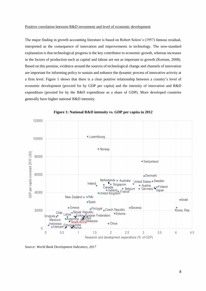
a firm level. Figure 1 shows that there is a clear positive relationship between a country’s level of
economic development (proxied for by GDP per capita) and the intensity of innovation and R&D
expenditure (proxied for by the R&D expenditure as a share of GDP). More developed countries
generally have higher national R&D intensity.
Figure 1: National R&D intensity vs. GDP per capita in 2012
Source: World Bank Development Indicators, 2017
9
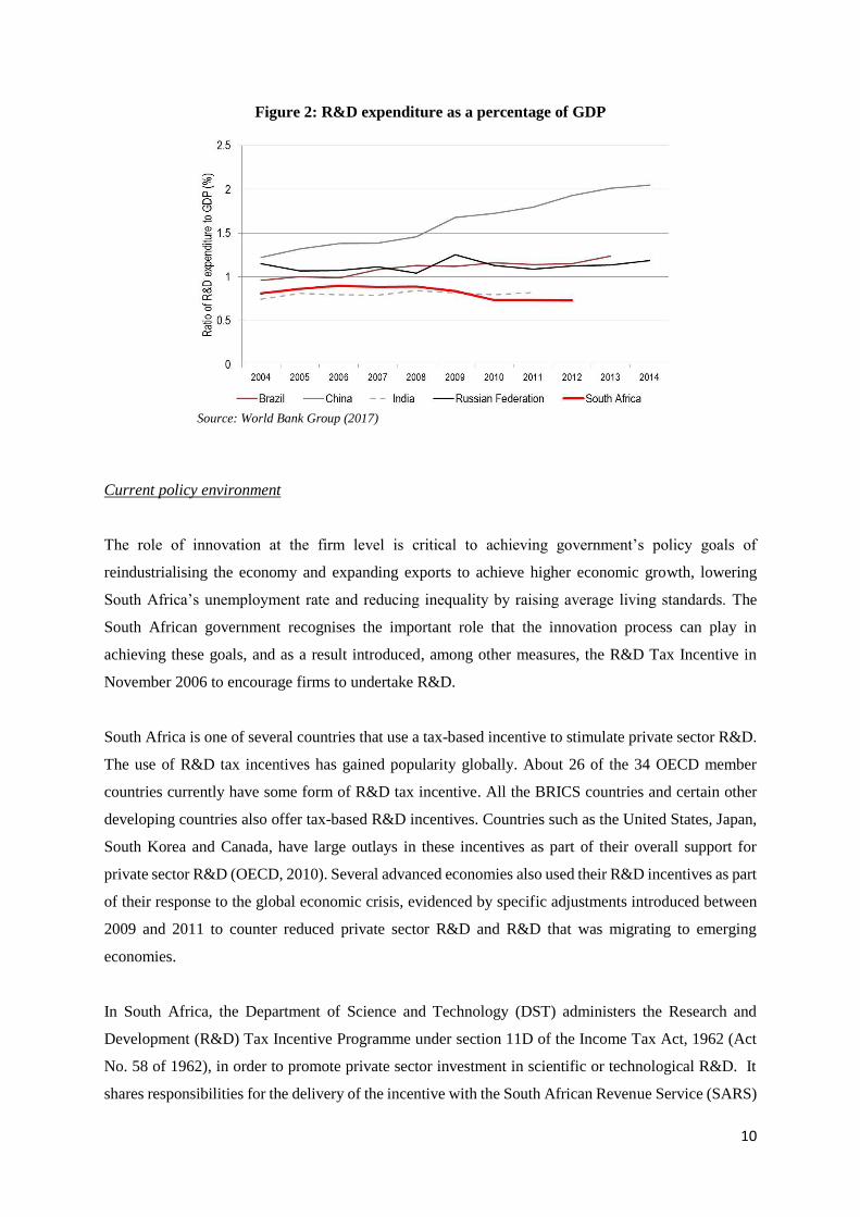
R&D expenditure relative to GDP in South Africa declined marginally over the period 2004 to 2012,
but increased in other emerging market peers including China, the Russian Federation and Brazil. The
ratio of R&D expenditure to GDP in South Africa – 0.73 per cent in 2012 – was the lowest among the
BRICS countries (e.g. China 1.93%, Brazil 1.15%). The Human Sciences Research Council (HSRC)
estimated that South Africa spent 0.73 per cent of its GDP on R&D in 2013/14 according to its R&D
survey, which compares unfavourably to an OECD average of 2.4 per cent of GDP.
3. South Africa has experienced weak productivity growth and a low share of R&D
expenditure to GDP
Most OECD countries are operating at the world technological frontier, where scope for rapid growth
through technology diffusion and catching-up is mostly gone. On the contrary, South Africa should be
growing faster than the OECD area and more in line with its emerging market peers as it industrialises
and grows; in part through adopting world-best technology. South Africa, however is caught in a cycle
of declining total factor productivity (TFP) growth and stagnant GDP growth at around 1 per cent. TFP
growth in its broadest sense is really technological change. While it is argued to be an imperfect measure
of innovation activity, it is a useful measure to ascertain an estimate of the level of investment in
innovation. When looking at trends in TFP growth over the period 1990 to 2015, South Africa mostly
lagged behind its BRICS5 peers, and since 2010 even experienced a contraction in TFP growth. A lack
of diversification of South Africa’s export basket over the period 1994 to 2015 also suggests that
product innovation is weak. As a result, South Africa would appear to be lagging in technological
progress relative to its emerging market peers. This is further reflected by the low share of high
technology exports as a percentage of manufactured exports compared to BRICS peers.
The number of trade patents is also lower than in the other BRICS. The exception is the mining and
fuels sub-sectors which have patents and R&D comparable to its competitors – the US, Canada and
Australia. Fostering innovation depends on effective Intellectual Property (IP) Rights Protection, for it
is difficult to have innovation without the protection of ideas. In the 2016/17 Global Competitiveness
Report, South Africa ranked 21st out of 138 countries for Intellectual Property Rights Protection, which
suggests that a sound legislative framework to support investment in innovation is in place. This raises
the question as to why innovation activity is so low compared to South Africa’s peers. Given the
importance of innovation for raising productivity and competitiveness in the long run, remaining stuck
at a low level of innovation activity in the economy is undesirable.
5 BRICS is the acronym for an association of five major emerging national economies: Brazil, Russia, India, China
and South Africa.
10
Figure 2: R&D expenditure as a percentage of GDP
Source: World Bank Group (2017)
Current policy environment
The role of innovation at the firm level is critical to achieving government’s policy goals of
reindustrialising the economy and expanding exports to achieve higher economic growth, lowering
South Africa’s unemployment rate and reducing inequality by raising average living standards. The
South African government recognises the important role that the innovation process can play in
achieving these goals, and as a result introduced, among other measures, the R&D Tax Incentive in
November 2006 to encourage firms to undertake R&D.
South Africa is one of several countries that use a tax-based incentive to stimulate private sector R&D.
The use of R&D tax incentives has gained popularity globally. About 26 of the 34 OECD member
countries currently have some form of R&D tax incentive. All the BRICS countries and certain other
developing countries also offer tax-based R&D incentives. Countries such as the United States, Japan,
South Korea and Canada, have large outlays in these incentives as part of their overall support for
private sector R&D (OECD, 2010). Several advanced economies also used their R&D incentives as part
of their response to the global economic crisis, evidenced by specific adjustments introduced between
2009 and 2011 to counter reduced private sector R&D and R&D that was migrating to emerging
economies.
In South Africa, the Department of Science and Technology (DST) administers the Research and
Development (R&D) Tax Incentive Programme under section 11D of the Income Tax Act, 1962 (Act
No. 58 of 1962), in order to promote private sector investment in scientific or technological R&D. It
shares responsibilities for the delivery of the incentive with the South African Revenue Service (SARS)

11
and the National Treasury. The incentive offers, among other benefits, a 150 per cent tax deduction for
approved R&D expenditure and can be accessed by companies of all sizes across all sectors of the
economy. From 1 Oct 2012, the procedure for administrating the R&D tax incentive changed from a
retrospective to pre-approval procedure, which based on anecdotal evidence, has resulted in application
backlogs, increased application complexity, and a general need to simplify the administrative process.
The incentive is part of a package of policy instruments to promote R&D and innovation in the country,
which the DST supports and oversees, including:
The Council for Scientific and Industrial Research (CSIR) is responsible for R&D in areas
including health, energy, advanced manufacturing and mining. An area of focus is its mining
research and technology development programme that aims to improve the competitiveness of
the local mining equipment manufacturing firms and also assist them develop products required
for narrow reef, hard rock mining; develop technological solutions that will increase the safety
and productivity, reduce the costs and ultimately extend the life of mines.
The Technology Innovation Agency (TIA) funds strategic technological innovation, emerging
technologies and knowledge innovation products with the aim of commercialising them.
The Technology for Human Resources in Industry Programme (THRIP) fosters R&D
collaboration between private-sector companies and universities and science councils.
The construction of MeerKAT, precursor to the Square Kilometre Array (SKA), has led to job
creation and diversification of the economy in the Northern Cape through DST’s technology
localisation strategy which requires 75 per cent local content in construction. SKA is the
department’s main infrastructure project and key contributor to current and future R&D.
The Support Programme for Industrial Innovation (SPII) and the Industrial Innovation
Partnership Programme (IIP).
Despite these efforts, South Africa needs to significantly increase investment and growth in R&D and
broadern innovation activity. The Minister of Science and Technology, Naledi Pandor, recently
announced a new R&D expenditure target of 1.5 per cent of GDP by 2019, more than double the current
spend.
4. Literature review: estimating the returns to R&D using firm-level data
There is a rich literature on measuring the contribution of R&D to TFP growth across a range of model
specifications and estimation methods, which Hall et al. (2009) summarise, and from which we draw
upon largely. One reason for such interest in this topic is that R&D investment is important for
improving the productivity and competitiveness of firms and the macro-economy. R&D can increase
12
productivity by improving the quality or reducing the average production costs of existing goods or
simply by widening the spectrum of final goods or intermediate inputs available (Hall et al., 2009).
Secondly, investment in R&D and innovation more broadly is generally expensive and diverts resources
away from other areas which may offer better short run gains or profitability. Any investment in R&D
and other innovation activities requires a long term view of improving productivity for movement closer
towards the productivity frontier at both a firm and economy wide level.
Modelling setup, approaches
The predominant approach that economists have taken to measure the return to firm’s investment in
R&D econometrically is the familiar growth accounting framework adapted with various measures of
R&D investment or capital at various levels of aggregation (Hall et al., 2009). According to Peters et
al. (2013), this work has been built for decades around the knowledge production function developed
by Griliches (1979). In this framework, firm investment in R&D creates a stock of knowledge within
the firm that enters into the firm’s production function as an additional input along with physical capital,
labor, and materials (Peters et al., 2013). The marginal product of this knowledge input provides a
measure of the return to the firm’s investment in R&D and has been the focus of the empirical
innovation literature (Peters et al., 2013). Model specifications are usually approximated by a Cobb-
Douglas production function in the three inputs, fixed capital stock C, labour L, and knowledge capital
K:
𝑌𝑖𝑡 = 𝐴𝑖𝑡𝐿𝑖𝑡𝛼 𝐶𝑖𝑡
𝛽𝐾𝑖𝑡
𝛾𝑒 𝑖𝑡 (1)
When applied to firm-level data, this framework relates output of a firm to either its stock of knowledge
capital and/or investment in R&D. Under this theoretical framework, two major approaches have been
followed: the primal approach6 and the dual approach7. In addition, Hall et al. (2009) point out that the
market value or Tobin’s q methodology is an important alternative approach taken in the literature,
which relates the current financial value of a firm to its underlying assets, including knowledge or R&D
assets. In some studies, additional information is added into the model such as producer behaviour and
market structure to allow for scale economies, mark-up pricing in the presence of imperfect competition
and intertemporal R&D investment decisions (Hall et al., 2009).
Econometric and data issues
6 This approach estimates a production function with quantities such as labour and capital as inputs. 7 The dual approach estimates a system of factor demand equations derived from a cost function representation of
technology (Hall et al., 2009). This approach assumes of some kind of optimising behaviour, such as profit
maximisation or cost minimisation, and then makes use of the theorems of duality to derive factor demand and
/or output supply equations.
13
There are numerous measurement issues raised in econometric studies of R&D and productivity. A key
area of concern is how to separate out the R&D effect from other explanatory factors of productivity.
Most studies measure output either by value added, sales or gross output, each of which has advantages
over the other. Cunѐo and Mairesse (1984) and Mairess and Hall (1994) find that the estimates of R&D
elasticities do not differ substantially when using either value added or sales (excluding materials/cost
of goods sold) as the dependent variable. Griliches and Mairesse (1984) find that when omitting
materials as an input from a estimation where sales is the dependent variable, an upward bias in the
R&D elasticity is likely because materials are correlated with R&D. The bias is more predictable in the
cross sectional dimension because the proportionality of materials to output is likely to hold, and is
roughly equal to the estimated R&D elasticity multiplied by materials share in output (Hall et al., 2009).
According to Hall et al. (2009), three issues particularly relevant to R&D arise when attempting to
correctly measure the elasticity of inputs in productivity analysis: (1) the R&D double-counting and
expensing bias in the estimated returns to R&D; (2) the sensitivity of these estimates to corrections for
quality differences in labour and capital, and (3) the sensitivity with respect to variations in capital
utilisation. The double-counting problem is that input factors such as labour, capital and material costs
are used in R&D activities, and hence R&D expenditures may be counted twice. A number of studies
attempt to measure this bias and make adjustments to ensure that input factors such as labour and capital
are cleared of their R&D components (Schankerman, 1981; Cunѐo and Mairesse, 1984; Hall and
Mairesse, 1995; Mairesse and Hall, 1994). Some of these studies find that there is a substantial
downward bias in the R&D elasticity when the adjustments to the inputs for R&D are not corrected for
in both the cross and time or within-firm dimensions. Some studies incorporate quality differences in
labour and capital into the production function. Mairesse and Cunéo (1985), Mairesse and Sassenou
(1989), and Crépon and Mairesse (1993) obtain lower R&D elasticities when different kinds of labour,
corresponding to different levels of educational qualifications are introduced separately into the
production function. Hall et al. (2009) argue that even through first differencing controls for permanent
differences across firms, it leaves too much cyclical noise and measurement error in the data, and
therefore the within firm rates of return to R&D are therefore difficult to estimate. Some studies use
long-differencing to remove part of this cyclical variation. Hall and Mairesse (1995) report more
significant R&D elasticities (but not rates of return) using long-differences rather than first-differenced
data.
Recent developments in this literature break away from the familiar knowledge production function
approach to measuring the private returns from R&D investment. Peters et al. (2013) develop and
estimate a dynamic, structural model of German manufacturing firm’s decision to invest in R&D and
quantify the cost and long-run benefit of this investment. The dynamic model incorporates and
14
quantifies linkages between the firm’s R&D investment, product and process innovations, and future
productivity and profits (Peters et al. 2013). Ski & Jaumandreu (2013) extend on the traditional
knowledge capital model of Griliches (1979) by developing a model of endogenous productivity change
to examine the impact of investment in knowledge on the productivity of firms.
An additional source of bias to estimates of the elasticity and returns to R&D are other factors that
contribute to technical progress such as returns to scale and technical change not directly as a direct
result of R&D. Hall et al. (2009) remark that controlling for time-invariant firm effects, the elasticities
and rates of return to R&D tend to be higher when constant returns to scale is imposed or when factor
elasticities are replaced by observed factor shares (see Griliches and Mairesse 1984, Cunéo and
Mairesse 1984, Griliches 1986, Griliches and Mairesse 1990, and Hall and Mairesse 1995). In addition,
it is argued that it is preferable to include time dummies when doing analysis at the firm level to account
for variations across time that may have little relationship to the R&D-productivity relationship, such
as macro-economic conditions, errors in deflators or other economy-wide measurement errors. Sector-
specific dummy variables can also be incorporated to account for firm-specific variations in
management or technological opportunity conditions.
An additional area of concern is that it is unlikely that R&D investment or expenditure becomes
productive immediately. It is very likely that there are lags of varying number of periods for R&D
investments to materialise into TFP growth. Various studies in the literature apply alternative lag
distributions, with most finding that the effect of R&D upon growth to begin on average in the second
to third year after the initial R&D input investment year and continues for several years after with
increasing influence (See Mansfield et al., 1971; Leonard, 1971; Ravenscraft and Scherer, 1982; Pakes
et al., 1984; Seldon, 1987; Geroski, 1989).
The definition of the sample from which to infer estimates could be susceptible to selection bias if only
R&D performing firms are included in the sample. Several studies look at both R&D and non-R&D
performing firms and find that the rate of return is not fundamentally different for the firms with and
without R&D (Mairesse and Cunéo, 1985; Mairesse and Sassenou, 1989; Crépon and Mairesse, 1993).
However, Klette (1994) reports that non-R&D performing firms have a lower productivity performance.
Hall and Mairesse (1995) apply several measures to remove extreme outliers from the sample to clean
their sample of US and French manufacturing firms from abnormally high or low observations. Hall et
al. (2009) point out that in certain studies, the estimates can be very sensitive to the removal of outliers.
Finally, simultaneity bias is possible in the estimate of the elasticity or rate of return to R&D from a
production function depending on the choice of output and inputs. Some studies use reduced form
specification estimates, as in Griliches & Mairesse (1984) and Hall & Mairesse (1995), to deal with this
15
bias. Others use instrumental variables or Generalised Method of Moments (GMM) techniques (Hall
and Mairesse, 1995; Klette, 1992; Bond et al., 2005; Griffith et al., 2006). Certain studies use beginning-
of-period instead of end-of-period R&D capital stock to account for potential simultaneity bias. Hall et
al. (2009) indicate that both Griliches and Mairesse (1984) and Mairesse and Hall (1994) find higher
R&D elasticities with end-of-period than with beginning-of-period R&D stocks (especially in the
within-firm dimension), because of the feedback from sales to current levels of investment.
5. Methodology, findings from other studies and data
Methodology and approach
We use a production function approach to estimate the returns to R&D, a theoretical framework which
is by far the predominant approach to estimating the return to R&D econometrically in the literature.
This framework essentially relates the residual growth factor in production that is not accounted for by
the usual factor inputs (i.e. labour, capital, intermediate inputs) to R&D that produces technical change
(Hall et al., 2009). We follow this standard theoretical framework primarily for the purpose of
comparing our results to literature surveyed by Hall et al. (2009), which is summarised briefly in the
previous section. Many of the data and model specification issues that we encounter using a production
function approach are not dissimilar to those encountered in the papers which use this standard model
setup surveyed by Hall et al. (2009). We are therefore able to compare our results to the literature more
closely than if we had used an alternative approach. For the same reason of comparability, we follow
Hall and Mairesse (1995) and Mairesse and Hall (1996) so closely. As in Hall and Mairesse (1995), we
assume that the production function for manufacturing firms can be approximated by a Cobb-Douglas
production function in the three inputs, fixed capital stock C, labour L, and knowledge capital K:
𝑌𝑖𝑡 = 𝐴𝑖𝑡𝐿𝑖𝑡𝛼 𝐶𝑖𝑡
𝛽𝐾𝑖𝑡
𝛾𝑒 𝑖𝑡 (1)
Y is value added or gross sales, ε is a multiplicative disturbance, i denotes firms and t years. Technical
change is captured by Ait which varies over time as well as across firms. We take logarithms when
estimating the Cobb-Douglas production function to obtain the following linear regression equation,
which can be easily estimated:
𝑦𝑖𝑡 = 𝜂𝑖 + 𝜆𝑡 + 𝛼𝑙𝑖𝑡 + 𝛽𝑐𝑖𝑡 + 𝛾𝑘𝑖𝑡 + 휀𝑖𝑡 (2)
16
Lower case letters denote the logarithms of variables. In this framework, we implicitly assume that the
log of technical progress (A) can be written as the sum of a sector or firm-specific effect 𝜂𝑖 and a time
effect 𝜆𝑡 (Hall et al., 2009). In practice we replace 𝜆𝑡 with year dummies.
There are two methods to estimate the return to R&D, which is the marginal product of R&D capital
(𝜌). In the first method, and the one which we present results for in this paper, we use simple algebra
manipulation of the identities below:
𝛾8 ≡ 𝜌𝐾𝑖𝑡
𝑌𝑖𝑡, hence 𝜌 ≡ 𝛾/
𝐾𝑖𝑡
𝑌𝑖𝑡
Therefore we can estimate the return to R&D by estimating 𝛾 (equation 2), the R&D capital intensity
ratio 𝐾
𝑌
(mean, median), and then use these two estimates to derive an estimate of the return to R&D,
which is:
�� = 𝛾/ (𝐾
𝑌)
(3)
We use this relationship as our main empirical strategy – a method which is standard in the literature.
An issue however with this method is that it is difficult to obtain a sufficient series of estimates of R&D
capital stock 𝐾𝑖𝑡 because a relatively long time series is required to cumulate R&D investment (𝑅𝑖𝑡)
and an assumed depreciation rate (𝛿) by the following equation:
𝐾𝑖𝑡 = 𝑅𝑖𝑡 − 𝛿𝐾𝑖𝑡−𝑡 (4)
We have a short panel with frequent gaps in the time series so are unable to construct cumulated R&D
capital 𝐾𝑖𝑡. As a solution to this problem, we follow Hall et al. (2009) in assuming a steady state growth
rate 𝑔𝑖𝑡 to approximate for 𝐾𝑖𝑡:
𝐾𝑖𝑡 ≈𝑅𝑖𝑡
𝛿+𝑔𝑖𝑡 (4)
E.g. if 𝛿 = 15% (typical) and 𝑔𝑖𝑡 = 5%, then 𝐾𝑖𝑡= 5 𝑅𝑖𝑡.
The benefit of using this approximation is that we can justify using R&D expenditure (flow variable)
instead of R&D capital stock in our estimations, which is the variable that we have available in the
dataset we use.
Our approach in estimating �� is to use all practical methods available taking into account data
constraints and benchmark these results against previous studies using firm level data from other
8 Elasticity of output with respect to R&D capital.
17
countries. This framework is evidently susceptible to simultaneity bias where the left hand side (value
added or gross sales) is determined jointly with variables on the right hand side, R&D in particular.
Moreover, the error term may include any errors in the specification which may arise because firms
have different production functions or because we have not disaggregated the inputs adequately enough,
as well as pure measurement error in any of the explanatory variables (Hall and Mairesse, 1995). We
adopt a number of 1996) to address these problems, which the methods used by Hall and Mairesse
(1995) and Mairesse and Hall (include: using the first lag instead of the current value of the stock of
fixed capital and the level of R&D expenditure, estimating 𝛾 using pooled OLS, fixed effects, first-
differences and long-differences. The latter estimation methods attempt to address the potential for
omitted variable bias by estimating after transforming equation (2) to eliminate the firm-specific
heterogeneity term 𝜂𝑖. However the problem with first-differences and fixed effects using annual data
is that it removes the firm-specific heterogeneity term, but aggravates any measurement error problem,
which is an area of concern in our estimations. This provides the motivation for using the long-
differences estimator, as it deals specifically with the familiar “measurement error in panel data”
problem discussed by Griliches and Hausman (1986). The long-differences estimator is essentially firm-
average-growth over the full available period, and because growth rates are averages, the measurement
error bias is reduced.9 We also, when doing these estimations, restrict our analysis to the manufacturing
sector, as it is argued by Hall and Mairesse (1996) that both labour productivity and total factor
productivity are better measured and more meaningful in the manufacturing sector that other sectors
(Mairesse and Hall, 1996). Several other firm level studies in the literature also restrict their analysis
only to manufacturing sector firms.
The second method estimates the marginal product of R&D capital (ρ) directly by estimating equation
(5) below using first differences:
∆𝑦𝑖𝑡 = ∆𝜆𝑡 + 𝛼∆𝑙𝑖𝑡 + 𝛽∆𝑐𝑖𝑡 + 𝜌 (𝑅𝑖𝑡− 𝛿𝐾𝑖𝑡−1
𝑌𝑖𝑡) + ∆휀𝑖𝑡 (5)
A problem highlighted by Hall et al. (2009) in the literature is that this approach generally understates
the estimates for 𝜌 and generates unstable estimates. Similarly, unstable estimates are also our
experience using this approach and so we do not report our results here.
Findings from other studies (mostly OECD countries)
9 In our dataset, we encounter a problem where we have many gaps in the time series dimension of the panel. In
cases like this, it is useful to use a long-differences estimator. The advantage of this technique is that we can
calculate average growth over a period even though there are gaps in the data.
18
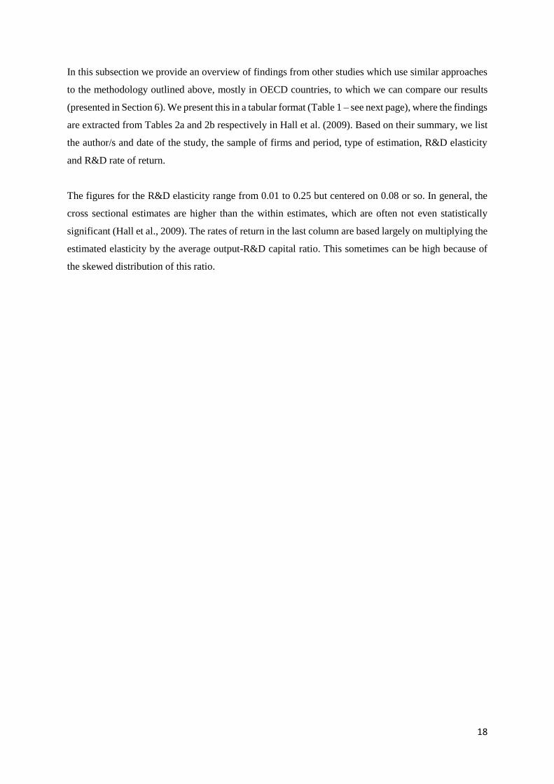
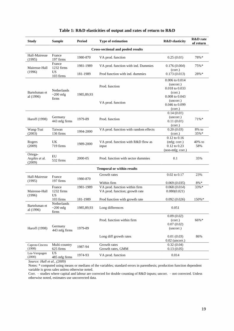
In this subsection we provide an overview of findings from other studies which use similar approaches
to the methodology outlined above, mostly in OECD countries, to which we can compare our results
(presented in Section 6). We present this in a tabular format (Table 1 – see next page), where the findings
are extracted from Tables 2a and 2b respectively in Hall et al. (2009). Based on their summary, we list
the author/s and date of the study, the sample of firms and period, type of estimation, R&D elasticity
and R&D rate of return.
The figures for the R&D elasticity range from 0.01 to 0.25 but centered on 0.08 or so. In general, the
cross sectional estimates are higher than the within estimates, which are often not even statistically
significant (Hall et al., 2009). The rates of return in the last column are based largely on multiplying the
estimated elasticity by the average output-R&D capital ratio. This sometimes can be high because of
the skewed distribution of this ratio.
19
Table 1: R&D elasticities of output and rates of return to R&D
Study Sample Period Type of estimation R&D elasticity R&D rate
of return
Cross-sectional and pooled results
Hall-Mairesse
(1995)
France
197 firms 1980-870 VA prod. function 0.25 (0.01) 78%*
Mairesse-Hall
(1996)
France
1232 firms
US
103 firms
1981-1989
181-1989
VA prod. function with ind. Dummies
Prod function with ind. dummies
0.176 (0.004)
(corr.)
0.173 (0.013)
75%*
28%*
Bartelsman et
al (1996)
Netherlands
~200 mfg
firms
1985,89,93
Prod. function
VA prod. function
0.006 to 0.014
(uncorr.)
0.018 to 0.033
(corr.)
0.008 to 0.043
(uncorr.)
0.046 to 0.099
(corr.)
Haroff (1998) Germany
443 mfg firms 1979-89 Prod. function
0.14 (0.01)
(uncorr.)
0.11 (0.01)
(corr.)
71%*
Wang-Tsai
(2003)
Taiwan
136 firms 1994-2000
VA prod. function with random effects
0.20 (0.03)
(corr.)
8% to
35%*
Rogers
(2009)
UK
719 firms 1989-2000
VA prod. function with R&D flow as
input
0.12 to 0.16
(mfg; corr.)
0.12 to 0.23
(non-mfg; corr.)
40% to
58%
Ortega-
Argilѐs et al.
(2009)
EU
532 firms 2000-05 Prod. function with sector dummies 0.1 35%
Temporal or within results
Hall-Mairesse
(1995)
France
197 firms 1980-870
Growth rates
Within firm
0.02 to 0.17
0.069 (0.035)
23%
8%*
Mairesse-Hall
(1996)
France
1232 firms
US
103 firms
1981-1989
181-1989
VA prod. function within firm
VA prod. function; growth rate
Prod function with growth rate
0.068 (0.014)
0.080(0.021)
0.092 (0.026)
33%*
150%*
Bartelsman et
al (1996)
Netherlands
~200 mfg
firms
1985,89,93 Long differences 0.051
Haroff (1998) Germany
443 mfg firms 1979-89
Prod. function within firm
Long diff growth rates
0.09 (0.02)
(corr.)
0.07 (0.02)
(uncorr.)
0.01 (0.03)
0.02 (uncorr.)
66%*
86%
Capron-Cincera (1998)
Multi-country
625 firms 1987-94
Growth rates
Growth rates, GMM
0.32 (0.04)
0.13 (0.05)
Los-Verspagen
(2000)
US
485 mfg firms 1974-93 VA prod. function 0.014
Source: Hall et al., (2009)
Notes: * computed using means or medians of the variables; standard errors in parenthesis; production function dependent
variable is gross sales unless otherwise noted.
Corr. – studies where capital and labour are corrected for double counting of R&D inputs; uncorr. – not corrected. Unless
otherwise noted, estimates use uncorrected data.
20
Data
We use the South African Revenue Service and National Treasury Firm-Level Panel (herein referred to
as SARS-NT panel), which is an unbalanced panel data set of administrative tax data from 2008 to 2016
at present. The SARS-NT dataset allows the first economy-wide investigation into the dynamics of
innovation in South Africa and the factors that affect firm-level decisions, and will allow us to test the
contribution of R&D expenditure to productivity growth as well as its intensity and persistence over
time in a more rigorous way than has been possible up to now. The analysis provides a useful
contribution to the literature from a developing country perspective, as most previous studies focus on
advanced or OECD countries.
The panel was created by merging four sources of administrative tax data received in 2015 that
constitute the panel which are: (i) company income tax from registered firms who submit tax forms; (ii)
employee data from employee income tax certificates submitted by employers; (iii) value-added tax
data from registered firms; and (iv) customs records from traders (Pieterse et al., 2016). These data sets
constitute a significant and unique source for the study of firm-level behaviour in post-apartheid South
Africa, as it is at the level of individual firms and individuals. The integrated dataset thus can be used
to provide a comprehensive, disaggregated picture of the economy over time. Detailed firm-level
analysis has not been adequately explored from a South African policy research perspective, partly as
the result of data unavailability in addition to data quality concerns. For our purposes we make use of
the company income tax records which contain firm characteristics, including financial information
from their income statements and balance sheets and tax information. In addition we draw from the
employee records from individual IRP5 and IT3a forms which contain employee related information
such as incomes, taxes and payments made by the firm (Pieterse et al., 2016). In this paper we make
particular use of recorded R&D expenditure, found in the income statements of firms over the period
2009 to 2014.
The definition of the R&D expenditure variable is comparable to the guidelines in the OECD Frascati
Manual, which is also the basis for the data used in most other studies. In short, firms are required to
report any expenses on scientific or technological research and development for (i) the discovery of
non-obvious information of a scientific and technological nature and (ii) the creating of any
interventions, any design or computer programme of knowledge (SARS, 2013).
There are several caveats to be noted when using this data. (1) When restricting the number of firms
that record both positive turnover and employment (have PAYE records), which differ per year, there
are roughly 200 000 to 250 000 of these firms each year (out of a total of 600 000 to 650 000 firms
registered per year). These numbers exclude body corporates, and about two thirds of ‘firms’ registered
21
for tax purposes – which have no turnover or other income source. (2) The definition of a ‘firm’ is
merely that of an entity registered for tax purposes – a company/group might have many ‘firms’
registered depending on how they structure their business. Some of these registrations with no turnover
are due to poorly filled out data, or because they are used for other tax purposes (e.g. complex group
structures, or shell companies where firms defray expenditure, or registered entities specifically set up
to hold assets and not be associated with the profit and loss account of the other companies in the group,
or be liable to be attached for legal purposes). (3) Employment numbers refer to ‘formally’ employed
individuals, where companies fill out IRP details, but are not far off official Statistics South Africa
Quarterly Employment Survey estimates. (4) The panel is short with many missing observations in the
time series, which renders it difficult or even impossible to create a cumulative time serious for certain
variables in the dataset. We restrict the period of analysis from 2009 to 2014 due to insufficient data
available in 2008, 2015 and 2016 at the time.
6. Variables and descriptive analysis
Variables in the SARS-NT panel used in our analysis
The variables we use are defined similarly to Hall and Mairesse (1995) and Mairesse and Hall (1996),
but adjusted where necessary according to limitations in the SARS-NT panel dataset. We use gross
sales; end-year book value of fixed capital (which includes property, plant and equipment); employment
from the individual IRP5 returns certificates; R&D expenditure; materials (defined as the cost of goods
sold); and value added (calculated as gross sales less the cost of goods sold). We use these variables to
calculate R&D intensity, measured as the ratio of R&D to sales in percentage terms. We generate the
logs of these variables for our productivity analysis. In addition, we compute these ratios using a one
year lag on sales and value added as per Hall and Mairesse (1995).
None of the variables are deflated. This is not a significant oversight as inflation was relatively low over
the period 2009 to 2014 (about 5% per annum) and the time dummy variables capture this variability
in part. It may be worthwhile to deflate output by an output deflator, fixed capital by an overall
investment deflator and R&D expenditure by a manufacturing sector level value added deflator as done
in Hall and Mairesse (1995).
Few firms report R&D expenditure in South Africa tax administrative data
Initially, we restrict our sample to firms which report positive values of gross sales and fixed capital in
a financial year. This leaves between 189 000 to 241 000 in the sample over the period 2009 to 2014
(Table 2 – see below). Only a small number of these firms report positive values of R&D expenditure,
22
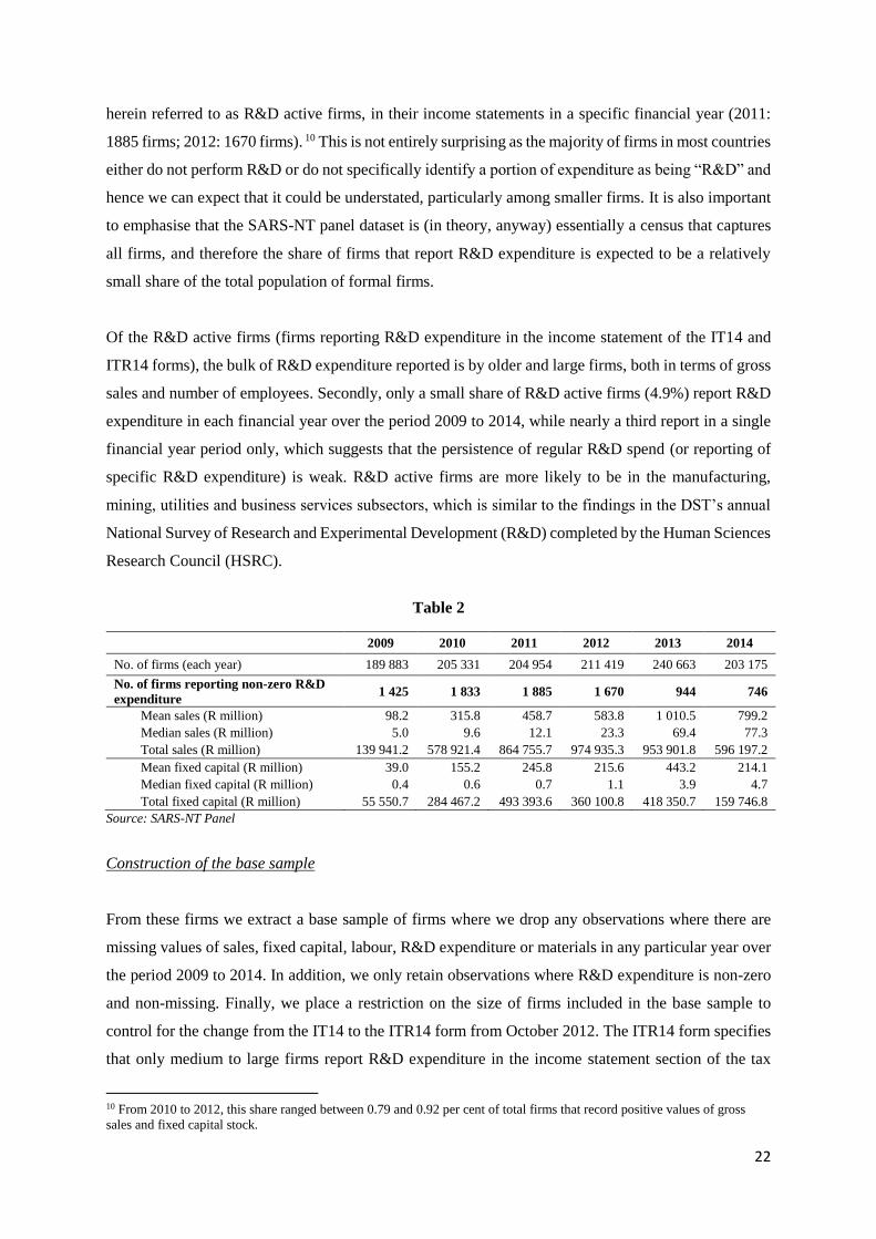
herein referred to as R&D active firms, in their income statements in a specific financial year (2011:
1885 firms; 2012: 1670 firms). 10 This is not entirely surprising as the majority of firms in most countries
either do not perform R&D or do not specifically identify a portion of expenditure as being “R&D” and
hence we can expect that it could be understated, particularly among smaller firms. It is also important
to emphasise that the SARS-NT panel dataset is (in theory, anyway) essentially a census that captures
all firms, and therefore the share of firms that report R&D expenditure is expected to be a relatively
small share of the total population of formal firms.
Of the R&D active firms (firms reporting R&D expenditure in the income statement of the IT14 and
ITR14 forms), the bulk of R&D expenditure reported is by older and large firms, both in terms of gross
sales and number of employees. Secondly, only a small share of R&D active firms (4.9%) report R&D
expenditure in each financial year over the period 2009 to 2014, while nearly a third report in a single
financial year period only, which suggests that the persistence of regular R&D spend (or reporting of
specific R&D expenditure) is weak. R&D active firms are more likely to be in the manufacturing,
mining, utilities and business services subsectors, which is similar to the findings in the DST’s annual
National Survey of Research and Experimental Development (R&D) completed by the Human Sciences
Research Council (HSRC).
Table 2
2009 2010 2011 2012 2013 2014
No. of firms (each year) 189 883 205 331 204 954 211 419 240 663 203 175
No. of firms reporting non-zero R&D
expenditure 1 425 1 833 1 885 1 670 944 746
Mean sales (R million) 98.2 315.8 458.7 583.8 1 010.5 799.2
Median sales (R million) 5.0 9.6 12.1 23.3 69.4 77.3
Total sales (R million) 139 941.2 578 921.4 864 755.7 974 935.3 953 901.8 596 197.2
Mean fixed capital (R million) 39.0 155.2 245.8 215.6 443.2 214.1
Median fixed capital (R million) 0.4 0.6 0.7 1.1 3.9 4.7
Total fixed capital (R million) 55 550.7 284 467.2 493 393.6 360 100.8 418 350.7 159 746.8
Source: SARS-NT Panel
Construction of the base sample
From these firms we extract a base sample of firms where we drop any observations where there are
missing values of sales, fixed capital, labour, R&D expenditure or materials in any particular year over
the period 2009 to 2014. In addition, we only retain observations where R&D expenditure is non-zero
and non-missing. Finally, we place a restriction on the size of firms included in the base sample to
control for the change from the IT14 to the ITR14 form from October 2012. The ITR14 form specifies
that only medium to large firms report R&D expenditure in the income statement section of the tax
10 From 2010 to 2012, this share ranged between 0.79 and 0.92 per cent of total firms that record positive values of gross
sales and fixed capital stock.
23
return, compared to the prior IT14 which allowed firms of all sizes to report such expenditure in the
income statement. Therefore only medium to large firms with total income greater than R14 million or
total assets exceeding R10 million are retained in the sample. This results in quite a number of micro
and small firms (all that record R&D expenditure) being dropped from the sample, particularly from
2009 to 2012 before the change to the ITR14 form. This however does not change our results in any
significant way. Both R&D intensity and R&D elasticity estimates change little. We also restrict the
period of analysis from 2009 to 2014, and drop any observations in 2008 and 2015 respectively because
of a limited number of observations reported in these financial years.
After placing these restrictions on the sample, an unbalanced sample of 1776 firms remain in the base
sample from 2009 to 2014 across several sectors of the economy. These firms record positive values of
R&D expenditure in at least one financial year period from 2009 to 2014. This sample of firms consists
of 3907 observations, as several of these firms report R&D expenditure is multiple years over the period
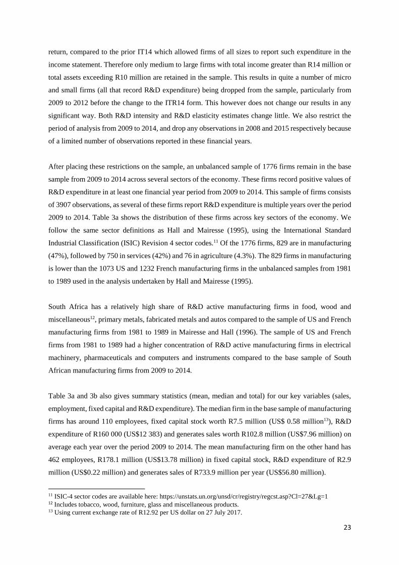
2009 to 2014. Table 3a shows the distribution of these firms across key sectors of the economy. We
follow the same sector definitions as Hall and Mairesse (1995), using the International Standard
Industrial Classification (ISIC) Revision 4 sector codes.11 Of the 1776 firms, 829 are in manufacturing
(47%), followed by 750 in services (42%) and 76 in agriculture (4.3%). The 829 firms in manufacturing
is lower than the 1073 US and 1232 French manufacturing firms in the unbalanced samples from 1981
to 1989 used in the analysis undertaken by Hall and Mairesse (1995).
South Africa has a relatively high share of R&D active manufacturing firms in food, wood and
miscellaneous12, primary metals, fabricated metals and autos compared to the sample of US and French
manufacturing firms from 1981 to 1989 in Mairesse and Hall (1996). The sample of US and French
firms from 1981 to 1989 had a higher concentration of R&D active manufacturing firms in electrical
machinery, pharmaceuticals and computers and instruments compared to the base sample of South
African manufacturing firms from 2009 to 2014.
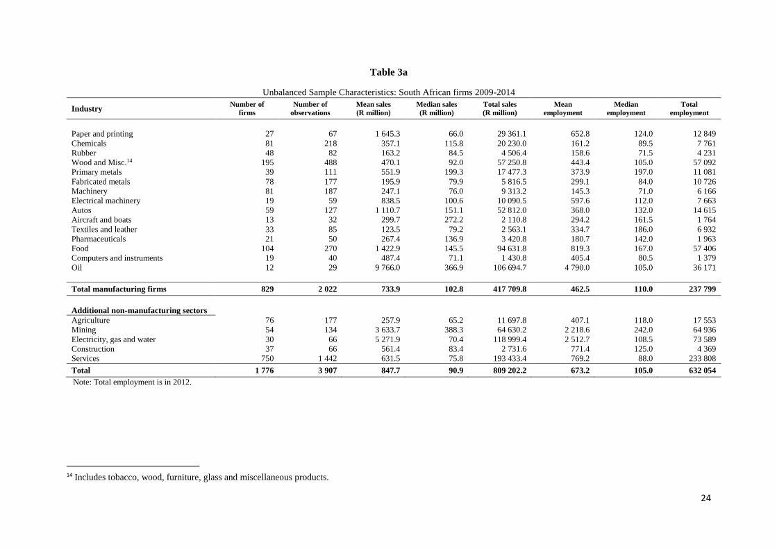
Table 3a and 3b also gives summary statistics (mean, median and total) for our key variables (sales,
employment, fixed capital and R&D expenditure). The median firm in the base sample of manufacturing
firms has around 110 employees, fixed capital stock worth R7.5 million (US$ 0.58 million13), R&D
expenditure of R160 000 (US$12 383) and generates sales worth R102.8 million (US$7.96 million) on
average each year over the period 2009 to 2014. The mean manufacturing firm on the other hand has
462 employees, R178.1 million (US$13.78 million) in fixed capital stock, R&D expenditure of R2.9
million (US$0.22 million) and generates sales of R733.9 million per year (US$56.80 million).
11 ISIC-4 sector codes are available here: https://unstats.un.org/unsd/cr/registry/regcst.asp?Cl=27&Lg=1 12 Includes tobacco, wood, furniture, glass and miscellaneous products. 13 Using current exchange rate of R12.92 per US dollar on 27 July 2017.
24
Table 3a
Unbalanced Sample Characteristics: South African firms 2009-2014
Industry Number of
firms
Number of
observations
Mean sales
(R million)
Median sales
(R million)
Total sales
(R million)
Mean
employment
Median
employment
Total
employment
Paper and printing 27 67 1 645.3 66.0 29 361.1 652.8 124.0 12 849
Chemicals 81 218 357.1 115.8 20 230.0 161.2 89.5 7 761
Rubber 48 82 163.2 84.5 4 506.4 158.6 71.5 4 231
Wood and Misc.14 195 488 470.1 92.0 57 250.8 443.4 105.0 57 092
Primary metals 39 111 551.9 199.3 17 477.3 373.9 197.0 11 081
Fabricated metals 78 177 195.9 79.9 5 816.5 299.1 84.0 10 726
Machinery 81 187 247.1 76.0 9 313.2 145.3 71.0 6 166
Electrical machinery 19 59 838.5 100.6 10 090.5 597.6 112.0 7 663
Autos 59 127 1 110.7 151.1 52 812.0 368.0 132.0 14 615
Aircraft and boats 13 32 299.7 272.2 2 110.8 294.2 161.5 1 764
Textiles and leather 33 85 123.5 79.2 2 563.1 334.7 186.0 6 932
Pharmaceuticals 21 50 267.4 136.9 3 420.8 180.7 142.0 1 963
Food 104 270 1 422.9 145.5 94 631.8 819.3 167.0 57 406
Computers and instruments 19 40 487.4 71.1 1 430.8 405.4 80.5 1 379
Oil 12 29 9 766.0 366.9 106 694.7 4 790.0 105.0 36 171
Total manufacturing firms 829 2 022 733.9 102.8 417 709.8 462.5 110.0 237 799
Additional non-manufacturing sectors
Agriculture 76 177 257.9 65.2 11 697.8 407.1 118.0 17 553
Mining 54 134 3 633.7 388.3 64 630.2 2 218.6 242.0 64 936
Electricity, gas and water 30 66 5 271.9 70.4 118 999.4 2 512.7 108.5 73 589
Construction 37 66 561.4 83.4 2 731.6 771.4 125.0 4 369
Services 750 1 442 631.5 75.8 193 433.4 769.2 88.0 233 808
Total 1 776 3 907 847.7 90.9 809 202.2 673.2 105.0 632 054
Note: Total employment is in 2012.
14 Includes tobacco, wood, furniture, glass and miscellaneous products.
25
Table 3b
Unbalanced Sample Characteristics: South African firms 2009-2014
Industry Mean fixed
capital
(R million)
Median fixed
capital
(R million)
Total fixed
capital
(R million)
Mean R&D
expenditure
(R million)
Median R&D
expenditure
(R million)
Total R&D
expenditure
(R million)
Mean R&D to
sales ratio
Median R&D to
sales ratio
Paper and printing 950.3 9.8 15 300.2 2.68 0.08 39.4 0.16 0.11
Chemicals 65.6 4.9 3 282.8 1.04 0.12 45.8 0.29 0.09
Rubber 34.6 12.9 1 139.9 0.32 0.09 8.9 0.19 0.11
Wood and Misc.15 106.5 7.3 14 777.2 2.32 0.14 381.2 0.48 0.12
Primary metals 107.6 12.6 2 284.7 1.03 0.16 38.2 0.19 0.07
Fabricated metals 35.2 7.9 2 214.6 0.65 0.10 8.4 0.33 0.12
Machinery 17.8 1.6 736.6 2.18 0.12 60.4 0.88 0.14
Electrical machinery 90.9 3.8 1 320.6 2.24 0.22 19.0 0.27 0.08
Autos 116.0 14.3 4 833.1 4.10 0.31 301.4 0.37 0.17
Aircraft and boats 32.1 9.9 98.1 12.63 0.42 164.7 4.22 0.14
Textiles and leather 12.2 6.0 242.3 0.41 0.14 6.3 0.33 0.12
Pharmaceuticals 29.8 10.2 416.5 4.61 0.66 47.9 1.57 0.46
Food 245.5 15.0 18 005.1 3.20 0.18 256.1 0.22 0.11
Computers and instruments 33.3 5.7 141.7 4.47 0.62 52.4 0.82 0.58
Oil 3 952.7 14.1 36 936.4 44.40 0.11 261.3 0.45 0.05
Total manufacturing firms 178.1 7.5 101 729.7 2.9 0.16 1 691.3 0.39 0.12
Additional non-manufacturing sectors
Agriculture 33.0 6.4 1 651.7 2.80 0.15 119.1 1.08 0.19
Mining 1 898.5 107.0 26 715.3 11.51 0.65 113.7 0.31 0.09
Electricity, gas and water 6 092.6 1.5 130 847.6 14.21 1.15 285.8 0.26 0.63
Construction 327.3 4.3 3 748.0 0.64 0.15 3.8 0.10 0.11
Services 384.8 2.5 67 882.0 1.81 0.16 503.2 0.22 0.16
Total 409.3 5.2 332 504.7 2.94 0.17 2 716.9 0.32 0.14
Note: Total fixed capital is in 2012. Mean R&D to sales ratio shown is the sales-weighted average over the period 2009-2014.
15 Includes tobacco, wood, furniture, glass and miscellaneous products.
26
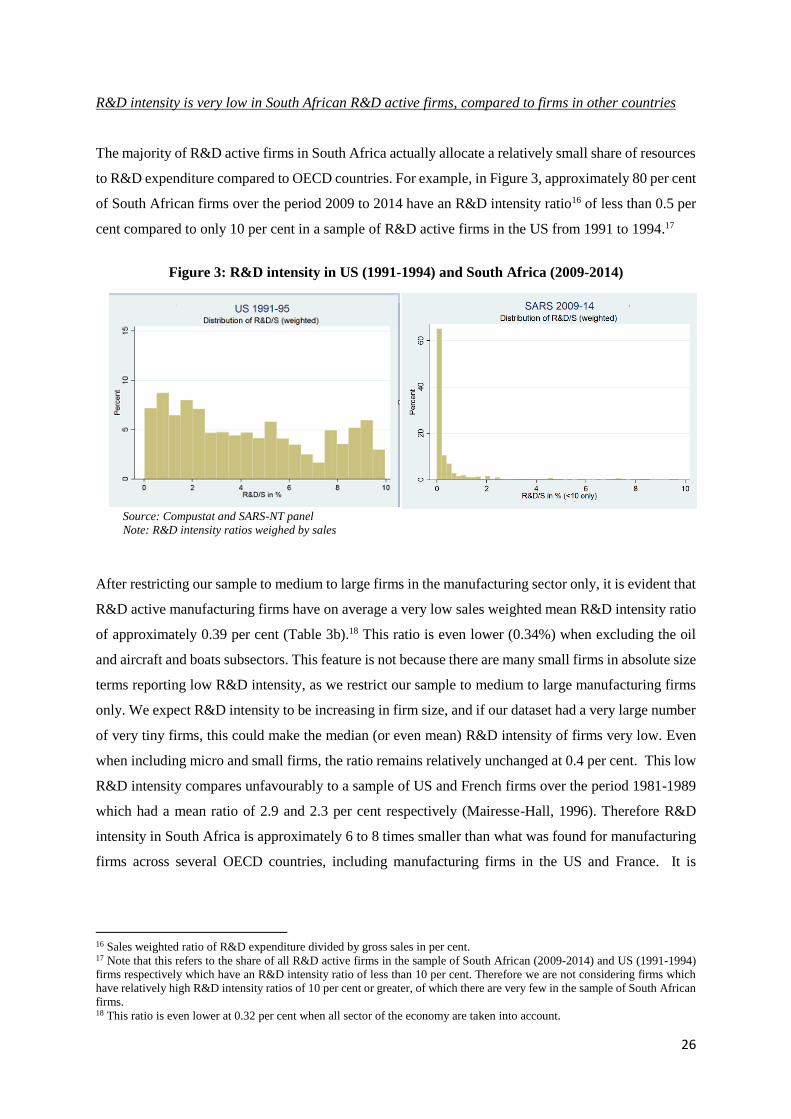
R&D intensity is very low in South African R&D active firms, compared to firms in other countries
The majority of R&D active firms in South Africa actually allocate a relatively small share of resources
to R&D expenditure compared to OECD countries. For example, in Figure 3, approximately 80 per cent
of South African firms over the period 2009 to 2014 have an R&D intensity ratio16 of less than 0.5 per
cent compared to only 10 per cent in a sample of R&D active firms in the US from 1991 to 1994.17
Figure 3: R&D intensity in US (1991-1994) and South Africa (2009-2014)
Source: Compustat and SARS-NT panel
Note: R&D intensity ratios weighed by sales
After restricting our sample to medium to large firms in the manufacturing sector only, it is evident that
R&D active manufacturing firms have on average a very low sales weighted mean R&D intensity ratio
of approximately 0.39 per cent (Table 3b).18 This ratio is even lower (0.34%) when excluding the oil
and aircraft and boats subsectors. This feature is not because there are many small firms in absolute size
terms reporting low R&D intensity, as we restrict our sample to medium to large manufacturing firms
only. We expect R&D intensity to be increasing in firm size, and if our dataset had a very large number
of very tiny firms, this could make the median (or even mean) R&D intensity of firms very low. Even
when including micro and small firms, the ratio remains relatively unchanged at 0.4 per cent. This low
R&D intensity compares unfavourably to a sample of US and French firms over the period 1981-1989
which had a mean ratio of 2.9 and 2.3 per cent respectively (Mairesse-Hall, 1996). Therefore R&D
intensity in South Africa is approximately 6 to 8 times smaller than what was found for manufacturing
firms across several OECD countries, including manufacturing firms in the US and France. It is
16 Sales weighted ratio of R&D expenditure divided by gross sales in per cent. 17 Note that this refers to the share of all R&D active firms in the sample of South African (2009-2014) and US (1991-1994)
firms respectively which have an R&D intensity ratio of less than 10 per cent. Therefore we are not considering firms which
have relatively high R&D intensity ratios of 10 per cent or greater, of which there are very few in the sample of South African
firms. 18 This ratio is even lower at 0.32 per cent when all sector of the economy are taken into account.
27
unsurprising that the number of firms undertaking and reporting R&D expenditure is low, however, the
low intensity of R&D among South African manufacturing firms is concerning.
At a manufacturing subsector level, the sales weighted mean R&D to sales ratio is highest in the aircraft
and boats (4.22%), pharmaceuticals (1.57%), machinery (0.88%) and computers and instruments
(0.82%) manufacturing subsectors. It appears that on average, this ratio is higher in the manufacturing
sector compared to other sectors in the economy, with exception to the agriculture sector which has a
relatively high ratio of 1.08 per cent. When comparing these ratios to those of US and French
manufacturing firms from 1981 to 1989 in Mairesse and Hall (1996), all South African manufacturing
subsectors report a lower ratio with exception to aircraft and boats, where South Africa reports a higher
ratio than the US (albeit comparing different time periods).
There are several plausible explanations for these findings. Firstly, it could be that there is under-
reporting of R&D expenditure which places a downward bias on the intensity of R&D activity among
South African manufacturing firms. This could be due to difficulties in either defining R&D activity or
isolating expenditure which aligns strictly within the definition of R&D provided. Firms therefore either
refrain from reporting their R&D expenditure or under report on it. On the other hand, it is also possible
that some firms do not adhere to the definition of R&D and over report R&D expenditure, in which
case the intensity of R&D expenditure may be biased upwards.
Secondly, the low intensity of R&D expenditure may be related to the fact that “R&D” may take on a
different nature in developing countries, where it is less easily defined compared to R&D activity in
developed countries. Countries that are not at the technological frontier engage more in activities that
“absorb” technologies established elsewhere, and this activity may not be counted explicitly as “R&D”
expenditure by the firm. Earlier research using the SARS-NT dataset suggests that in South Africa there
is a positive correlation between importing intermediate goods directly and exporting.19 This link is
strengthened by increasing the variety of imports and by importing from developed rather than emerging
markets. Where intermediates are imported from appears to also affect the productivity of firms – with
imports from developed countries having a large positive effect – due to technology and knowledge
transfer. This suggests that the channel of increasing productivity may be through technology transfer
embodied in the imports, and that many of these firms may be part of global value chains, instead of
R&D activity originating in South Africa. This suggests that policies that restrict imports, or raise the
costs of intermediates, may hinder exports and productivity growth. It also suggests that integrating into
global value chains may raise productivity, or having higher productivity may preclude the ability of
firms to join value chains (depending on how the chain originates in South Africa). Importing from a
19 See Edwards, L., Sanfilippo, M., A. Sundaram (2016). Importing and firm performance: New evidence from South Africa.
WIDER Working Paper 2016-039. Helsinki: UNU-WIDER. See also Matthee, M., N. Rankin, T. Naughtin, and C.
Bezuidenhout (2016). The South African manufacturing exporter story. WIDER Working Paper 2016-038. Helsinki: UNU-
WIDER.
28
variety of sources also appears to be critical for raising productivity and export growth. This suggests
that one should be careful when trying to restrict imports from particular regions (or when risking trade
policy retaliation through aggressive policy moves), and should not focus only in very narrow
preferential or regional trade agreements.
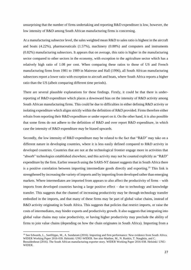
Lastly, it may be that our findings are for the most part accurate, and that the intensity of R&D
expenditure is genuinely low in South Africa. To test our findings with other data, we analysed R&D
expenditure data from listed companies on the Johannesburg Stock Exchange (JSE) from 2012 to 2016.
Although this data is not exactly comparable to the SARS-NT dataset, the trends that emerge are very
similar – low R&D intensity and a relatively low share of listed firms investing in R&D each year. Only
around 11 to 12 per cent of firms listed on the JSE invested in R&D annually over the period 2012 to
2016. These results validate the SARS-NT sample basic features but with named companies, capturing
the leading R&D firms. It is particularly striking that the distribution of R&D intensity is identical to
the distribution in the SARS-NT sample, which validates our findings considerably. It is also worth
noting that the JSE sample definition is perhaps more comparable to the sample of firms in Mairesse
and Hall (1996) than the SARS-NT sample we use, as the US sample consists of listed firms, so there
are not very many small firms.
Figure 4: Distribution of R&D intensity of JSE listed firms (2012-2016) and Top 10 companies -
R&D intensity average (2012-2016)
Source: McGregor Database, 2017. Note: R&D intensity ratios weighed by sales
Persistence of regular R&D expenditure is weak based on firm-level evidence
Over the full period, the number of observations across manufacturing firms is 2002, considerably less
than the 6521 and 6282 observations in the sample of American and French firms used in Mairesse and
Hall (1996). This is despite the number of manufacturing firms in the South African sample being fairly
comparable to the US and French samples (South Africa: 829 firms; US: 1073 firms; France: 1232
firms). This suggests a low persistence of R&D expenditure among R&D active firms in South Africa
Company R&D Intensity (%)
Silverbridge Holdings 9.856448
Psg Konsult Limited 4.497555
Taste Hldgs Ltd 2.615601
Adcock Ingram Hldgs Ltd 1.620435
Purple Group Ltd 1.233805
Anchor Group Limited 1.1123
Reunert Ltd 0.934902
Avi Ltd 0.587605
Compagnie Fin Richemont 0.575759
Anglo American Plat Ltd 0.556895
29
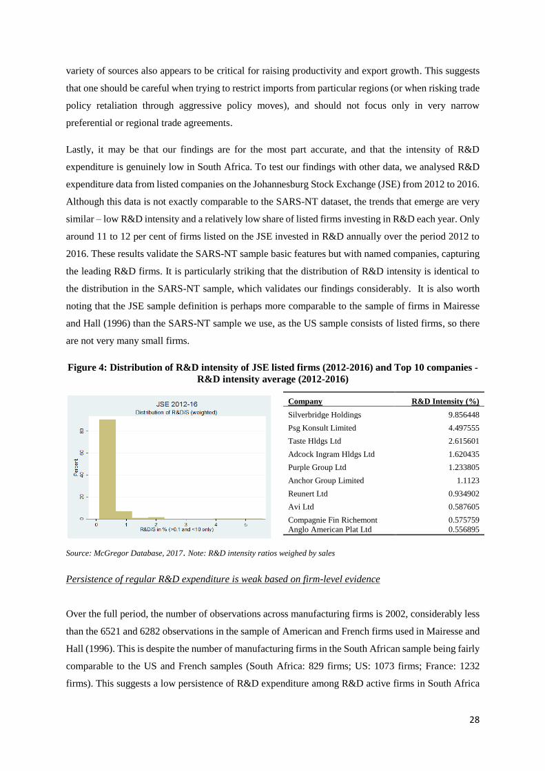
compared to the US and French samples. To quantify and account for this, we construct 3-4-5 year
balanced panels over the following periods: 2012 to 2014; 2011 to 2014; and 2010 to 2014. Of the 829
manufacturing firms in the unbalanced panel sample from 2009 to 2014, only 155 consistently report
R&D expenditure in each year over the 3-year period from 2012 to 2014. Table 4 shows that this
number decreases further in the 4-year and 5-year balanced panels to 121 and 86 firms over the period
2011 to 2014 and 2010 to 2014 respectively.
Table 4
Number of firms by panel sample
Industry Unbalanced
sample
3-year
balanced
(2012-2014)
4-year
balanced
(2011-2014)
5-year
balanced
(2010-2014)
Paper and Printing 27 8 6 2
Chemicals 81 13 10 9
Rubber 48 2 2 1
Wood and Misc.20 195 46 35 23
Primary metals 39 13 13 12
Fabricated metals 78 11 5 2
Machinery 81 12 10 6
Electrical machinery 19 7 6 5
Autos 59 5 4 2
Aircraft and boats 13 4 3 3
Textiles and leather 33 6 5 5
Pharmaceuticals 21 1 1 1
Food 104 21 17 11
Computers and instruments 19 4 2 2
Oil 12 2 2 2
Total manufacturing firms 829 155 121 86
Additional non-manufacturing sectors
Agriculture 76 12 10 6
Mining 54 9 8 3
Electricity, gas and water 30 4 3 2
Construction 37 3 2 2
Services 750 79 59 37
Total 1 776 262 203 136
Note: For each balanced panel sample, the distribution of firms reflected is in 2012. The distribution changes
marginally across years for the balanced panels, most likely due to firms changing their reported sector in
subsequent tax submissions.
R&D active firms are on average larger employers than non-active R&D firms
Another interesting descriptive feature is that South African R&D active firms are on average larger
employers than non-active R&D firms. Manufacturing firms (excluding the oils and aircraft and boats
subsectors) that recorded R&D expenditure over the period 2009 to 2014 had a mean employment value
of 319.5 compared to 59.1 for non-active R&D firms in the sector. Although it is reasonable to expect
that this is driven by a disproportionately large number of small non-active R&D firms with few
20 Includes tobacco, wood, furniture, glass and miscellaneous products.
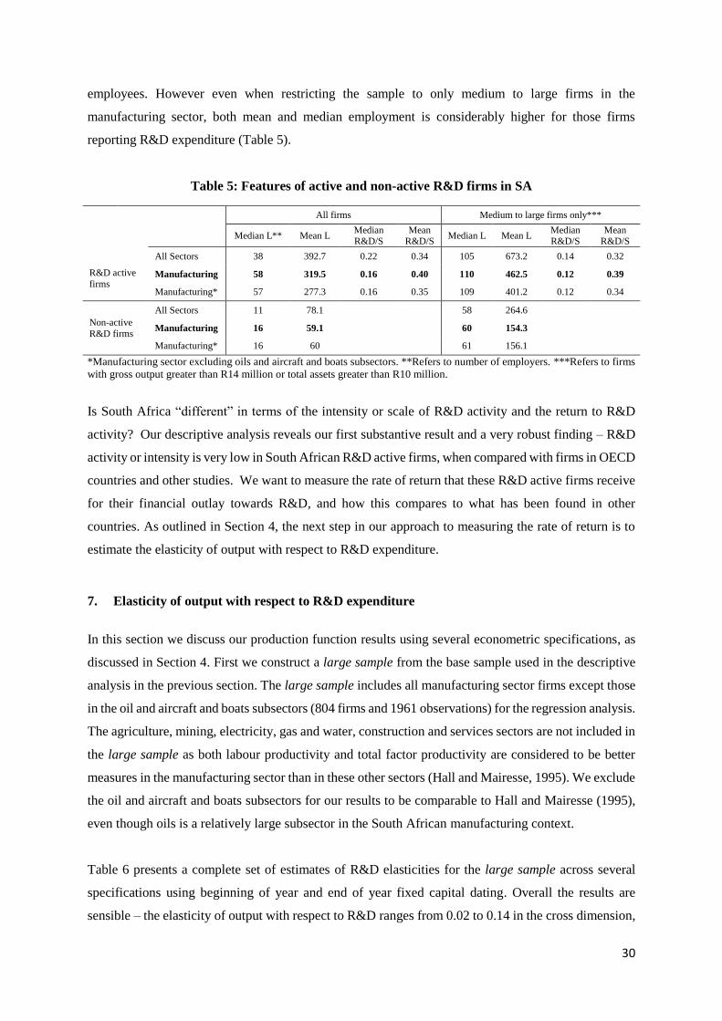
30
employees. However even when restricting the sample to only medium to large firms in the
manufacturing sector, both mean and median employment is considerably higher for those firms
reporting R&D expenditure (Table 5).
Table 5: Features of active and non-active R&D firms in SA
All firms Medium to large firms only***
Median L** Mean L
Median R&D/S
Mean R&D/S
Median L Mean L Median R&D/S
Mean R&D/S
R&D active
firms
All Sectors 38 392.7 0.22 0.34 105 673.2 0.14 0.32
Manufacturing 58 319.5 0.16 0.40 110 462.5 0.12 0.39
Manufacturing* 57 277.3 0.16 0.35 109 401.2 0.12 0.34
Non-active
R&D firms
All Sectors 11 78.1 58 264.6
Manufacturing 16 59.1 60 154.3
Manufacturing* 16 60 61 156.1
*Manufacturing sector excluding oils and aircraft and boats subsectors. **Refers to number of employers. ***Refers to firms
with gross output greater than R14 million or total assets greater than R10 million.
Is South Africa “different” in terms of the intensity or scale of R&D activity and the return to R&D
activity? Our descriptive analysis reveals our first substantive result and a very robust finding – R&D
activity or intensity is very low in South African R&D active firms, when compared with firms in OECD
countries and other studies. We want to measure the rate of return that these R&D active firms receive
for their financial outlay towards R&D, and how this compares to what has been found in other
countries. As outlined in Section 4, the next step in our approach to measuring the rate of return is to
estimate the elasticity of output with respect to R&D expenditure.
7. Elasticity of output with respect to R&D expenditure
In this section we discuss our production function results using several econometric specifications, as
discussed in Section 4. First we construct a large sample from the base sample used in the descriptive
analysis in the previous section. The large sample includes all manufacturing sector firms except those
in the oil and aircraft and boats subsectors (804 firms and 1961 observations) for the regression analysis.
The agriculture, mining, electricity, gas and water, construction and services sectors are not included in
the large sample as both labour productivity and total factor productivity are considered to be better
measures in the manufacturing sector than in these other sectors (Hall and Mairesse, 1995). We exclude
the oil and aircraft and boats subsectors for our results to be comparable to Hall and Mairesse (1995),
even though oils is a relatively large subsector in the South African manufacturing context.
Table 6 presents a complete set of estimates of R&D elasticities for the large sample across several
specifications using beginning of year and end of year fixed capital dating. Overall the results are
sensible – the elasticity of output with respect to R&D ranges from 0.02 to 0.14 in the cross dimension,
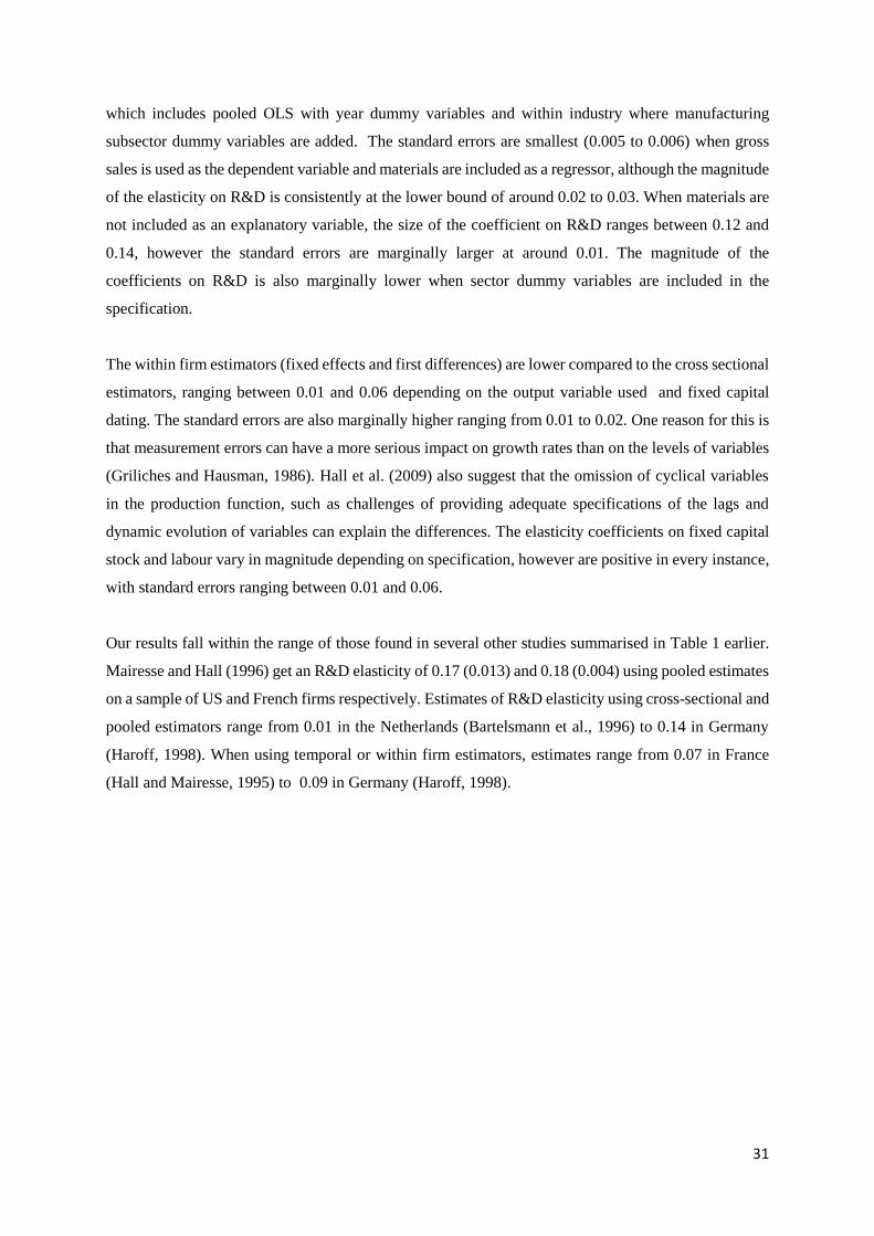
31
which includes pooled OLS with year dummy variables and within industry where manufacturing
subsector dummy variables are added. The standard errors are smallest (0.005 to 0.006) when gross
sales is used as the dependent variable and materials are included as a regressor, although the magnitude
of the elasticity on R&D is consistently at the lower bound of around 0.02 to 0.03. When materials are
not included as an explanatory variable, the size of the coefficient on R&D ranges between 0.12 and
0.14, however the standard errors are marginally larger at around 0.01. The magnitude of the
coefficients on R&D is also marginally lower when sector dummy variables are included in the
specification.
The within firm estimators (fixed effects and first differences) are lower compared to the cross sectional
estimators, ranging between 0.01 and 0.06 depending on the output variable used and fixed capital
dating. The standard errors are also marginally higher ranging from 0.01 to 0.02. One reason for this is
that measurement errors can have a more serious impact on growth rates than on the levels of variables
(Griliches and Hausman, 1986). Hall et al. (2009) also suggest that the omission of cyclical variables
in the production function, such as challenges of providing adequate specifications of the lags and
dynamic evolution of variables can explain the differences. The elasticity coefficients on fixed capital
stock and labour vary in magnitude depending on specification, however are positive in every instance,
with standard errors ranging between 0.01 and 0.06.
Our results fall within the range of those found in several other studies summarised in Table 1 earlier.
Mairesse and Hall (1996) get an R&D elasticity of 0.17 (0.013) and 0.18 (0.004) using pooled estimates
on a sample of US and French firms respectively. Estimates of R&D elasticity using cross-sectional and
pooled estimators range from 0.01 in the Netherlands (Bartelsmann et al., 1996) to 0.14 in Germany
(Haroff, 1998). When using temporal or within firm estimators, estimates range from 0.07 in France
(Hall and Mairesse, 1995) to 0.09 in Germany (Haroff, 1998).
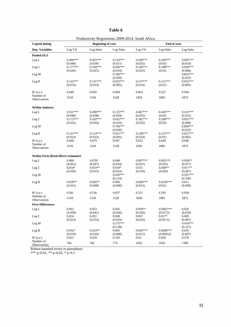
32
Table 6
Productivity Regressions 2009-2014, South Africa
Capital dating Beginning of year End of year
Dep. Variables Log VA Log Sales Log Sales Log VA Log Sales Log Sales
Pooled OLS
Log L 0.494*** 0.455*** 0.116*** 0.438*** 0.418*** 0.095*** (0.040) (0.039) (0.017) (0.035) (0.03) (0.014) Log C 0.177*** 0.194*** 0.030*** 0.182*** 0.198*** 0.030*** (0.026) (0.025) (0.010) (0.023) (0.02) (0.008)
Log M 0.786*** 0.803*** (0.028) (0.023)
Log R 0.132*** 0.121*** 0.025*** 0.137*** 0.121*** 0.025*** (0.014) (0.014) (0.005) (0.014) (0.01) (0.005)
R² (s.e.) 0.640 0.656 0.944 0.603 0.627 0.944
Number of Observations
1518 1536 1528 1858 1883 1872
Within Industry
Log L 0.531*** 0.490*** 0.125*** 0.467*** 0.445*** 0.101*** (0.040) (0.038) (0.018) (0.035) (0.03) (0.015)
Log C 0.175*** 0.182*** 0.032*** 0.181*** 0.189*** 0.031*** (0.025) (0.024) (0.010) (0.022) (0.02) (0.008) Log M 0.784*** 0.804*** (0.030) (0.023)
Log R 0.121*** 0.114*** 0.021*** 0.128*** 0.115*** 0.021*** (0.014) (0.014) (0.005) (0.014) (0.01) (0.005)
R² (s.e.) 0.660 0.679 0.947 0.622 0.649 0.946
Number of Observations
1518 1536 1528 1858 1883 1872
Within Firm (fixed effects estimator)
Log L 0.080 0.078* 0.049 0.097*** 0.092*** 0.038** (0.061) (0.047) (0.034) (0.031) (0.025) (0.017)
Log C 0.054* 0.033** 0.019* 0.031 0.048** 0.017** (0.030) (0.015) (0.010) (0.019) (0.020) (0.007) Log M 0.429*** 0.501*** (0.123) (0.106)
Log R 0.038** 0.020** 0.006 0.046*** 0.0229*** 0.011 (0.015) (0.008) (0.008) (0.013) (0.01) (0.008)
R² (s.e.) 0.581 0.526 0.937 0.521 0.293 0.938 Number of
Observations 1518 1536 1528 1858 1883 1872
First Differences
Log L 0.062 0.053 0.045 0.058** 0.0462*** 0.026 (0.058) (0.041) (0.036) (0.026) (0.0173) (0.019)
Log C 0.024 0.022 0.008 0.007 0.0177 0.009 (0.023) (0.014) (0.010) (0.016) (0.0115) (0.007)
Log M 0.373*** 0.414*** (0.138) (0.127) Log R 0.032* 0.023** 0.005 0.043*** 0.0268*** 0.010 (0.019) (0.010) (0.008) (0.015) (0.00832) (0.007)
R² (s.e.) 0.023 0.029 0.330 0.03 0.059 0.578 Number of
Observations 766 782 774 1033 1056 1398
Robust standard errors in parenthesis
*** p<0.01, ** p<0.05, * p<0.1
33
Data cleaning
To test the robustness of the estimation results of the large sample, we construct several additional sub-
samples by cleaning the data for various outliers and placing additional restrictions on which
manufacturing firms are included. We follow the approach taken by Hall and Mairesse (1995) and
Mairesse and Hall (1996) to clean the data. We apply this to the large sample according to the following
criteria:
1) We remove any observations where value added is zero or negative, as this creates problems
for the logarithmic specification. This removes 53 observations, which is 3 per cent of the base
sample of 1776 observations.
2) We then apply an interquartile range-based trimming on the unlogged values of value added
per worker, sales per worker, fixed capital per worker and R&D expenditure per worker. We
remove any observations that are outside three times the interquartile range above or below the
median.
3) We remove any observations for which the growth rates of sales, employment or fixed capital
are less than minus 50 per cent or greater than 200 per cent. In addition, we remove observations
where the growth rate in value added is less than minus 90 per cent or greater than 300 per cent.
The number of observations and firms in each of the five samples we use in the regression analysis are
shown below in
Table 7, where the various restrictions and cleaning criteria applicable to each sample are summarised.
Table 7
Description of samples used in the regression analysis
Sample Description of sample Number of
observations
Number of
firms
Large Manufacturing sector firms but excluding oil and
aircraft and boats subsectors 1961 804
hm95clean
Large sample excluding observations where:
VA per worker<=0
IQR-based trimming of the values of value added
per worker, sales per worker, fixed capital per
worker and R&D per worker.
Growth rates of sales, employment and fixed
capital less than -50% or greater than 200%.
Growth rate of value added less than -90% or
greater than 300%.
1245 465
mh96clean
Large sample excluding observations where:
VA per worker<=0
Growth rates of sales, employment and fixed
capital less than -50% or greater than 200%.
Growth rate of value added less than -90% or
greater than 300%.
1533 578
Large incl. aircraft and
boats Large sample including aircraft and boats subsector. 1993 817
Large incl. R&D/Sales
ratio>0.1%
Large sample including observations where the R&D to
sales ratio is greater than 0.1%. 1075 410
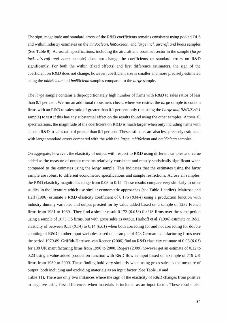
34
The sign, magnitude and standard errors of the R&D coefficients remains consistent using pooled OLS
and within industry estimates on the mh96clean, hm95clean, and large incl. aircraft and boats samples
(See Table 9). Across all specifications, including the aircraft and boast subsector in the sample (large
incl. aircraft and boats sample) does not change the coefficients or standard errors on R&D
significantly. For both the within (fixed effects) and first difference estimators, the sign of the
coefficient on R&D does not change, however, coefficient size is smaller and more precisely estimated
using the mh96clean and hm95clean samples compared to the large sample.
The large sample contains a disproportionately high number of firms with R&D to sales ratios of less
than 0.1 per cent. We run an additional robustness check, where we restrict the large sample to contain
firms with an R&D to sales ratio of greater than 0.1 per cent only (i.e. using the Large and R&D/S>0.1
sample) to test if this has any substantial effect on the results found using the other samples. Across all
specifications, the magnitude of the coefficient on R&D is much larger when only including firms with
a mean R&D to sales ratio of greater than 0.1 per cent. These estimates are also less precisely estimated
with larger standard errors compared with the with the large, mh96clean and hm95clean samples.
On aggregate, however, the elasticity of output with respect to R&D using different samples and value
added as the measure of output remains relatively consistent and mostly statistically significant when
compared to the estimates using the large sample. This indicates that the estimates using the large
sample are robust to different econometric specifications and sample restrictions. Across all samples,
the R&D elasticity magnitudes range from 0.03 to 0.14. These results compare very similarly to other
studies in the literature which use similar econometric approaches (see Table 1 earlier). Mairesse and
Hall (1996) estimate a R&D elasticity coefficient of 0.176 (0.004) using a production function with
industry dummy variables and output proxied for by value-added based on a sample of 1232 French
firms from 1981 to 1989. They find a similar result 0.173 (0.013) for US firms over the same period
using a sample of 1073 US firms, but with gross sales as output. Harhoff et al. (1996) estimate an R&D
elasticity of between 0.11 (0.14) to 0.14 (0.01) when both correcting for and not correcting for double
counting of R&D in other input variables based on a sample of 443 German manufacturing firms over
the period 1979-89. Griffith-Harrison-van Reenen (2006) find an R&D elasticity estimate of 0.03 (0.01)
for 188 UK manufacturing firms from 1990 to 2000. Rogers (2009) however get an estimate of 0.12 to
0.23 using a value added production function with R&D flow as input based on a sample of 719 UK
firms from 1989 to 2000. These finding hold very similarly when using gross sales as the measure of
output, both including and excluding materials as an input factor (See Table 10 and
Table 11). There are only two instances where the sign of the elasticity of R&D changes from positive
to negative using first differences when materials is included as an input factor. These results also
35
remain relatively consistent across different samples when using long differences to estimate the
elasticity of R&D (See Table 8).
Table 8
Productivity Regressions using Long Differences 2009-2014
Sample Large mh96clean hm95clean Large incl.
aircraft and boats
Large and
R&D/S>0.1
Dependent Variable: Value added
Log L 0.099*** 0.230*** 0.299*** 0.099*** 0.087** (0.032) (0.056) (0.068) (0.032) (0.039)
Log C 0.023 0.073** 0.132 0.023 0.012 (0.022) (0.035) (0.040) (0.022) (0.032)
Log M
Log R 0.084*** 0.020* 0.024* 0.088*** 0.134*** (0.014) (0.011) (0.012) (0.014) (0.020)
R² (s.e.) 0.031 0.028 0.049 0.027 0.073
Number of
Observations 1117 944 784 1135 636
Dependent Variable: Sales
Log L 0.036*** 0.110*** 0.149*** 0.036*** 0.043** (0.013) (0.028) (0.036) (0.013) (0.018)
Log C 0.026 0.056 0.087 0.026*** 0.032** (0.009) (0.017) (0.021) (0.009) (0.015)
Log M 0.655*** 0.487*** 0.414*** 0.659*** 0.508*** (0.020) (0.022) (0.025) (0.020) (0.030) Log R 0.032*** 0.005 0.003 0.033*** 0.040*** (0.006) (0.005) (0.006) (0.005) (0.009)
R² (s.e.) 0.524 0.468 0.432 0.523 0.524 Number of
Observations 1119 943 783 1138 638
Dependent Variable: Sales
Log L 0.080*** 0.136*** 0.198*** 0.081*** 0.072 (0.023) (0.040) (0.046) (0.023) (0.025)
Log C 0.060*** 0.066*** 0.103*** 0.061*** 0.058*** (0.016) (0.025) (0.028) (0.016) (0.020) Log M
Log R 0.041*** -0.002 0.002 0.045*** 0.081*** (0.001) (0.008) (0.008) (0.010) (0.012)
R² (s.e.) 0.034 0.026 0.051 0.032 0.076 Number of
Observations 1120 944 784 1139 638
Robust standard errors in parenthesis
*** p<0.01, ** p<0.05, * p<0.1
8. Summary of findings
Our empirical strategy to estimating the returns to R&D in South Africa is essentially comparative. We
obtain estimates of R&D intensity that we can compare to those obtained in previous studies (as
previously noted, largely relating to firms in OECD countries). We also use estimation methods that are
comparable to those used in these earlier studies. The measurement and estimation issues that have
beset previous researchers are present for us as well, but this also allows us to compare our results
directly to these studies. In summary, we find that: (1) R&D intensity, as measured by the R&D to sales
ratio, in South African manufacturing firms is considerably lower than that observed in previous studies;
36
(2) the elasticity of output with respect to R&D is within the range observed in previous studies; (3) as
a simple matter of arithmetic – since the return to R&D is the elasticity times the inverse of the R&D
intensity – (1) and (2) imply that the estimated return to R&D in South Africa is high compared to that
found for other countries. The worked example below to calculate the estimated return to R&D using
the theoretical framework discussed in Section 4 demonstrates these findings.
Worked example
Estimating the R&D intensity ratio (𝑲
𝒀)
Using the approximation used in the literature surveyed by Hall et al. (2009):
𝐾𝑖𝑡 ≈ 5 𝑅𝑖𝑡
𝐾
𝑌
≈ 5 ∗
𝑅
𝑆𝑎𝑙𝑒𝑠 ≈ 5 ∗ 0.34 ≈ 1.7%
𝐾
𝑌
≈ 5 ∗
𝑅
𝑉𝑎𝑙𝑢𝑒 𝑎𝑑𝑑𝑒𝑑 ≈ 5 ∗ 1.2 ≈ 6%21
Estimating the marginal product of R&D capital (��)
�� = 𝛾/ (𝐾
𝑌)
and 𝛾 (estimate of the elasticity of output with respect to R&D) is estimated to range between 0.02 to
0.14 using either sales or value added as the measure of output across a range of estimation techniques.
Therefore assuming 𝛾 = 0.02 and 𝐾
𝑌
= 0.017 (using sales as output), then
�� = 𝛾/ (𝐾
𝑌)
= 1.18 (implying a rate of return of 118%)
Assuming 𝛾 = 0.05 and 𝐾
𝑌
= 0.017 (using sales as output), then
�� = 𝛾/ (𝐾
𝑌)
= 2.94 (implying a rate of return of 294%)
21 Generally the R&D intensity ratio using value added is 2 to 3 times the ratio when sales is used as the measure of output in
the denominator. We find this using the SARS-NT data.
37
Assuming 𝛾 = 0.02 and 𝐾
𝑌
= 0.06 (using value added as output), then
�� = 𝛾/ (𝐾
𝑌)
= 0.33 (implying a rate of return of 33.3%)
Assuming 𝛾 = 0.14 and 𝐾
𝑌
= 0.06 (using value added as output), then
�� = 𝛾/ (𝐾
𝑌)
= 2.33 (implying a rate of return of 233%)
Typical results from studies using this method (via 𝛾) generate a R&D elasticity ranging from 0.05 to
0.25 if value added is used to measure output, and from 0.02 to 0.15 if sales is used to measure output.
These studies mostly find a rate of return of R&D of between 20 to 80 per cent (predominantly OECD
countries). Therefore the implied rate of return to R&D in South Africa is high by international
standards. Intuitively this makes sense, given the low prevalence, persistence and intensity of R&D of
those firms that do R&D in South Africa.
There are a number of interpretations for these results. Firstly, it may be that our findings are genuine
– the return to R&D is very high in South Africa compared to other countries. Secondly, it could be
because of an upward bias that operates in South Africa but not (or not to anything like the same extent)
in the countries/datasets in the other studies surveyed in HMM and cited here. The leading culprit for
this would be omitted variable bias, and specifically innovative activity that is not being recorded as
R&D. We raised the point earlier that R&D activity, and innovative activity in general, in firms in a
catching-up country that is not at the technological frontier may be different from that in firms that are
at the frontier. For this reason, R&D expenditure that we have recorded from firms may not accurately
reflect the true level of R&D activity and innovation taking place in firms more broadly. It is also
possible that both of these explanations are true, since they aren’t mutually exclusive.
9. Policy implications and conclusion
From a global perspective, there has been a persistent slowdown in productivity growth over recent
decades in many advanced economies, and more recently, this slowdown has extended to emerging
economies (OECD, 2016). This is concerning given that productivity gains are considered a central
driver of long-term improvements in living standards. It is argued that to boost productivity growth,
policy action to address the obstacles to knowledge and technology diffusion is required, while
continuing to support technological progress and innovation at the frontier. Understanding the dynamics
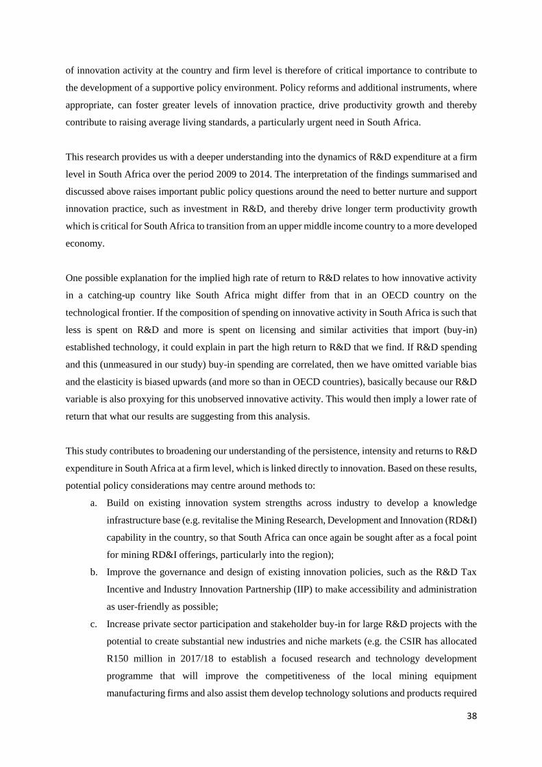
38
of innovation activity at the country and firm level is therefore of critical importance to contribute to
the development of a supportive policy environment. Policy reforms and additional instruments, where
appropriate, can foster greater levels of innovation practice, drive productivity growth and thereby
contribute to raising average living standards, a particularly urgent need in South Africa.
This research provides us with a deeper understanding into the dynamics of R&D expenditure at a firm
level in South Africa over the period 2009 to 2014. The interpretation of the findings summarised and
discussed above raises important public policy questions around the need to better nurture and support
innovation practice, such as investment in R&D, and thereby drive longer term productivity growth
which is critical for South Africa to transition from an upper middle income country to a more developed
economy.
One possible explanation for the implied high rate of return to R&D relates to how innovative activity
in a catching-up country like South Africa might differ from that in an OECD country on the
technological frontier. If the composition of spending on innovative activity in South Africa is such that
less is spent on R&D and more is spent on licensing and similar activities that import (buy-in)
established technology, it could explain in part the high return to R&D that we find. If R&D spending
and this (unmeasured in our study) buy-in spending are correlated, then we have omitted variable bias
and the elasticity is biased upwards (and more so than in OECD countries), basically because our R&D
variable is also proxying for this unobserved innovative activity. This would then imply a lower rate of
return that what our results are suggesting from this analysis.
This study contributes to broadening our understanding of the persistence, intensity and returns to R&D
expenditure in South Africa at a firm level, which is linked directly to innovation. Based on these results,
potential policy considerations may centre around methods to:
a. Build on existing innovation system strengths across industry to develop a knowledge
infrastructure base (e.g. revitalise the Mining Research, Development and Innovation (RD&I)
capability in the country, so that South Africa can once again be sought after as a focal point
for mining RD&I offerings, particularly into the region);
b. Improve the governance and design of existing innovation policies, such as the R&D Tax
Incentive and Industry Innovation Partnership (IIP) to make accessibility and administration
as user-friendly as possible;
c. Increase private sector participation and stakeholder buy-in for large R&D projects with the
potential to create substantial new industries and niche markets (e.g. the CSIR has allocated
R150 million in 2017/18 to establish a focused research and technology development
programme that will improve the competitiveness of the local mining equipment
manufacturing firms and also assist them develop technology solutions and products required

39
for narrow reef, hard rock mining, increase mine safety and productivity and reduce the costs
that will ultimately extend the life of mines);
d. Improve access to local and export markets through a combination of industry spending (e.g.
export credit financing that is not cross-cutting) and investment that enhances the quality of
and access to logistics infrastructure to lower logistics costs for firms;
e. Expand on the availability of early stage funding and establish sectoral innovation funding
instruments to address technology and innovation issues within sectors, based on joint public-
private funding.

40
10. References
Andrews, D., Criscuolo, C., & Gal, P. (2016) The Global Productivity Slowdown, Technology
Divergence and Public policy: A Firm Level Perspective. Preliminary OECD Background Paper.
Baba, Y. (1985) 'Japanese Colour TV Finns. Decision-making from the 1950s to the 1980s', DPhil
dissertation, Brighton, University of Sussex
Bartelsman, E. J., G. van Leeuwen, H. Nieuwenhuijsen, and K. Zeelenberg (1996), R&D and
productivity growth: evidence from firm-level data for the Netherlands. Netherlands Official Statistics
11 (Autumn), 52-69.
Bond, S., D. Harhoff, and J. Van Reenen (2003), Corporate R&D and Productivity in Germany and
the United Kingdom, Annales d’Economie et Statistique 79/80.
Crépon, B. and J. Mairesse (1993), Recherche et développement, qualification et productivité des
entreprises, in D. Guellec (ed.), Innovations et compétivité, INSEE-Méthodes no. 37-38, Paris:
Economica.
Cunéo, P. and J. Mairesse (1984), Productivity and R&D at the firm level in French manufacturing, in
Z. Griliches (ed.), R&D, Patents and Productivity. Chicago, IL: University of Chicago Press, 375-
392.
Ski, U.D. & Jaumandreu, J. (2013) R&D and Productivity: Estimating Endogenous Productivity.
Review of Economic Studies (2013) 80, 1338-1383.
Freeman, C. (1987) Technology Policy and Economic Performance: Lessons from Japan, London,
Frances Pinter
Freeman, C. (1995), The ‘National System of Innovation’ in historical perspective. Cambridge
Journal of Economics, 19, 5-24
Geroski, P. A. (1989), Entry, Innovation and Productivity Growth. Review of Economics and Statistics
71(4), 572-578.
Griffith, R., R. Harrison, and J. Van Reenen (2006), How Special Is the Special Relationship? Using
the Impact of U.S. R&D Spillovers On U.K. Firms As a Test of Technology Sourcing, American
Economic Review, 96(5), 1859-1875.
Griliches, Z. (1986), Productivity, R&D, and Basic Research At the Firm Level in the 1970s,
American Economic Review, 76, 141-154.
Griliches, Z., and J. Mairesse (1984), Productivity and R&D At the Firm Level, in R&D, Patents, and
Productivity, Ed. By Z. Griliches. Chicago, Ill.: Chicago University Press, 339-374.
Griliches, Z., and J. A. Hausman (1986), Errors in Variables in Panel Data. Journal of Econometrics
31 (1), 93-118.
Griliches, Z., and J. Mairesse (1990), R&D and Productivity Growth: Comparing Japanese and U. S.
Manufacturing Firms, in Productivity Growth in Japan and the United States, Ed. By C. R.
Hulten. Chicago: Chicago University Press, 317-340.
Griffith, R., R. Harrison, and J. Van Reenen (2006), How Special Is the Special Relationship? Using
the Impact of U.S. R&D Spillovers On U.K. Firms As a Test of Technology Sourcing, American
41
Economic Review, 96(5), 1859-1875.
Hall, B.H. & Mairesse, J. (1995) Exploring the relationship between R&D and productivity in French
manufacturing firms. Journal of Econometrics, 65 (1995), 263-293.
Hall, B.H., Mairesse, J. & Mohnen, P. (2009) Measuring the Returns to R&D. In: B. Hall & N.
Rosenberg, eds., Handbook of the Economics of Innovation, Amsterdam: Elsevier, Chapter 24.
HSRC. (2014) National Innovation Survey 2013/14
Harhoff, D. (1998), R&D and productivity in German manufacturing firms, Economics of Innovation
and New Technology, 6(1), 29-49.
Klette, T. J. (1994), R&D, scope economies, and company structure: a 'not so fixed effect' model of
plant performance. Oslo, Norway: Central Bureau of Statistics Discussion Paper No. 120.
Kortum, S. (2008) Exploring Innovation with Firm Level Data. [Online] Paper prepared for the
Conference Board’s Workshop Perspectives on U.S. Innovation and Competitiveness, February 8 and
9, 2007.
Leonard, W. N. (1971), Research and development in industrial growth, Journal of Political Economy
79(2), 232-56.
Mairesse, J., and P. Cunéo (1985), Recherche-développement et performances des entreprises: Une
étude économétrique sur données individuelles. Revue économique 36 (5), 1001-1041.
Mairesse, J., and B. H. Hall (1994), Estimating the Productivity of R&D in French and U.S.
Manufacturing Firms: An Exploration of Simultaneity Issues With GMM, in International
Productivity Comparisons, Ed. By K. Wagner. Amsterdam: Elsevier-North Holland.
Mairesse, J. & Hall, B.H. (1996) Estimating the Effect of Research and Development: An Exploration
of GMM Methods Using Data on French and United States Manufacturing Firms. NBER Working
Paper Series, Working Paper 5501 (March 1996).
Mairesse, J., and M. Sassenou (1989), Les facteurs qualitatifs de la productivité : un essai
d’évaluation. Economie et Prévision 91 (5), 35-42.
Mansfield, E., J. Rapoport, J. Schnee, S. Wagner, and M. Hamburger (1971), Research and
Development in the Modern Corporation. New York: W. W. Norton.
OECD (1996c), Technology and Industrial Performance, Paris.
OECD (1997) National Innovation Systems, OECD Publishing, Paris
OECD (2015), Frascati Manual 2015: Guidelines for Collecting and Reporting Data on Research and
Experimental Development, The Measurement of Scientific, Technological and Innovation Activities,
OECD Publishing, Paris. DOI: http://dx.doi.org/10.1787/9789264239012-en
OECD (2016) “The Productivity Inclusiveness Nexus”, OECD Publishing, Paris
Pakes, A., and M. Schankerman (1984), The rate of obsolescence of patents, research gestation lags,
and the private rate of return to research resources. In R&D, Patents, and Productivity, edited by Z.
Griliches. Chicago, IL: Chicago University Press, 73-88.
42
Peters, B., Roberts, M.J., Anh Vuong, V. & Fryges, H. (2013) Estimating Dynamic R&D Demand:
An Analysis of Costs and Long-Run Benefits. Discussion Paper No. 13-089.
http://ftp.zew.de/pub/zew-docs/dp/dp13089.pdf
Pieterse, D., Kreuser, C.F. & Gavin, E. (2016) Introduction to the South African Revenue Service
and National Treasury firm-level panel. Available at:
https://www.wider.unu.edu/sites/default/files/wp2016-42.pdf.
Ravenscraft, D. J., and F. M. Scherer (1982), The Lag Structure of Returns to Research and
Development. Applied Economics 14, 603-620.
Rogers, M. (2009), R&D and productivity: Using UK firm-level data to inform policy. Empirica. DOI
10.1007/s10663-009-9111-x.
SARS (2013) Comprehensive guide to the ITR14 return for companies.
Schankerman, M. (1981), The Effect of Double Counting and Expensing on the Measured Returns to
R&D. Review of Economics and Statistics 63(3), 454-458.
Seldon, B. (1987), A Nonresidual Estimation of Welfare Gains from Research: The Case of Public
R&D in a Forest Product Industry, Southern Economic Journal, 54(2), 64-80.
Takeuchi, H. and Nonaka, I. 1986. The new product development game, Harvard Business Review,
January/February, 285-305
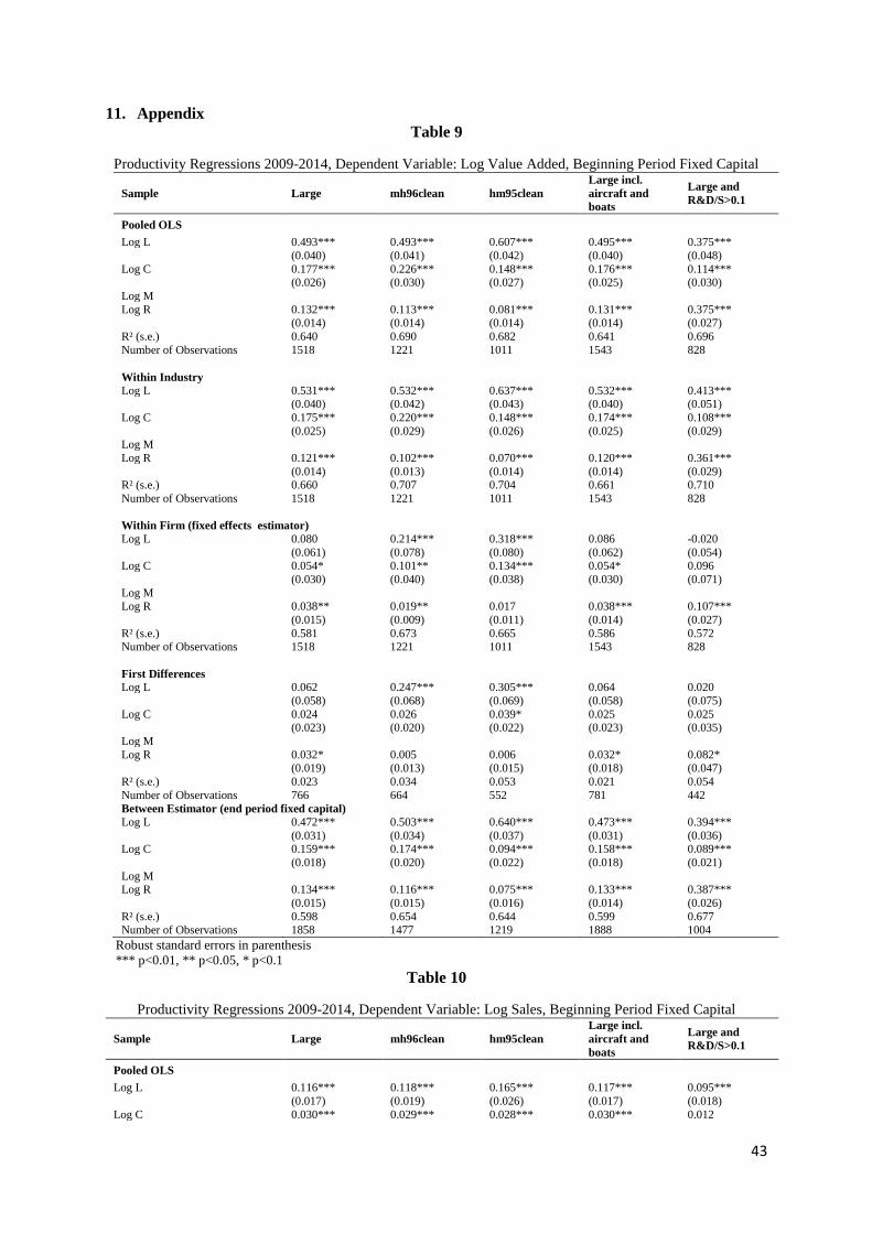
43
11. Appendix
Table 9
Productivity Regressions 2009-2014, Dependent Variable: Log Value Added, Beginning Period Fixed Capital
Sample Large mh96clean hm95clean
Large incl.
aircraft and
boats
Large and
R&D/S>0.1
Pooled OLS
Log L 0.493*** 0.493*** 0.607*** 0.495*** 0.375*** (0.040) (0.041) (0.042) (0.040) (0.048)
Log C 0.177*** 0.226*** 0.148*** 0.176*** 0.114*** (0.026) (0.030) (0.027) (0.025) (0.030)
Log M
Log R 0.132*** 0.113*** 0.081*** 0.131*** 0.375*** (0.014) (0.014) (0.014) (0.014) (0.027)
R² (s.e.) 0.640 0.690 0.682 0.641 0.696
Number of Observations 1518 1221 1011 1543 828
Within Industry
Log L 0.531*** 0.532*** 0.637*** 0.532*** 0.413*** (0.040) (0.042) (0.043) (0.040) (0.051)
Log C 0.175*** 0.220*** 0.148*** 0.174*** 0.108*** (0.025) (0.029) (0.026) (0.025) (0.029) Log M
Log R 0.121*** 0.102*** 0.070*** 0.120*** 0.361*** (0.014) (0.013) (0.014) (0.014) (0.029) R² (s.e.) 0.660 0.707 0.704 0.661 0.710
Number of Observations 1518 1221 1011 1543 828
Within Firm (fixed effects estimator)
Log L 0.080 0.214*** 0.318*** 0.086 -0.020 (0.061) (0.078) (0.080) (0.062) (0.054) Log C 0.054* 0.101** 0.134*** 0.054* 0.096 (0.030) (0.040) (0.038) (0.030) (0.071)
Log M
Log R 0.038** 0.019** 0.017 0.038*** 0.107*** (0.015) (0.009) (0.011) (0.014) (0.027)
R² (s.e.) 0.581 0.673 0.665 0.586 0.572 Number of Observations 1518 1221 1011 1543 828
First Differences
Log L 0.062 0.247*** 0.305*** 0.064 0.020 (0.058) (0.068) (0.069) (0.058) (0.075)
Log C 0.024 0.026 0.039* 0.025 0.025 (0.023) (0.020) (0.022) (0.023) (0.035)
Log M
Log R 0.032* 0.005 0.006 0.032* 0.082* (0.019) (0.013) (0.015) (0.018) (0.047)
R² (s.e.) 0.023 0.034 0.053 0.021 0.054
Number of Observations 766 664 552 781 442
Between Estimator (end period fixed capital)
Log L 0.472*** 0.503*** 0.640*** 0.473*** 0.394*** (0.031) (0.034) (0.037) (0.031) (0.036) Log C 0.159*** 0.174*** 0.094*** 0.158*** 0.089*** (0.018) (0.020) (0.022) (0.018) (0.021)
Log M
Log R 0.134*** 0.116*** 0.075*** 0.133*** 0.387*** (0.015) (0.015) (0.016) (0.014) (0.026)
R² (s.e.) 0.598 0.654 0.644 0.599 0.677 Number of Observations 1858 1477 1219 1888 1004
Robust standard errors in parenthesis
*** p<0.01, ** p<0.05, * p<0.1
Table 10
Productivity Regressions 2009-2014, Dependent Variable: Log Sales, Beginning Period Fixed Capital
Sample Large mh96clean hm95clean
Large incl.
aircraft and
boats
Large and
R&D/S>0.1
Pooled OLS
Log L 0.116*** 0.118*** 0.165*** 0.117*** 0.095*** (0.017) (0.019) (0.026) (0.017) (0.018)
Log C 0.030*** 0.029*** 0.028*** 0.030*** 0.012
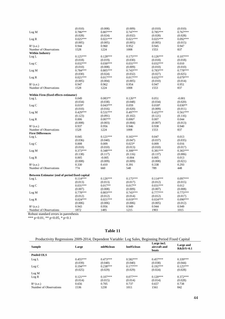
44
(0.010) (0.008) (0.009) (0.010) (0.010)
Log M 0.786*** 0.807*** 0.747*** 0.785*** 0.767*** (0.028) (0.024) (0.032) (0.028) (0.028)
Log R 0.025*** 0.021*** 0.021*** 0.025*** 0.092*** (0.005) (0.005) (0.005) (0.005) (0.015) R² (s.e.) 0.944 0.960 0.952 0.945 0.947
Number of Observations 1528 1224 1008 1553 837
Within Industry
Log L 0.125*** 0.128*** 0.175*** 0.126*** 0.107*** (0.018) (0.019) (0.030) (0.018) (0.018)
Log C 0.032*** 0.030*** 0.031*** 0.032*** 0.010 (0.010) (0.008) (0.009) (0.010) (0.010)
Log M 0.784*** 0.805*** 0.743*** 0.783*** 0.778*** (0.030) (0.024) (0.032) (0.027) (0.025) Log R 0.021*** 0.017*** 0.017*** 0.032*** 0.079*** (0.005) (0.004) (0.005) (0.010) (0.014)
R² (s.e.) 0.947 0.962 0.954 0.947 0.951 Number of Observations 1528 1224 1008 1553 837
Within Firm (fixed effects estimator)
Log L 0.049 0.083** 0.126** 0.051 -0.001 (0.034) (0.038) (0.048) (0.034) (0.020)
Log C 0.019* 0.043*** 0.059 0.018* 0.030** (0.010) (0.016) (0.020) (0.009) (0.011)
Log M 0.429*** 0.531*** 0.497*** 0.432*** 0.561*** (0.123) (0.091) (0.102) (0.121) (0.116) Log R 0.006 0.007** 0.006* 0.007 0.044 (0.008) (0.003) (0.004) (0.007) (0.013) R² (s.e.) 0.937 0.956 0.946 0.938 0.940
Number of Observations 1528 1224 1008 1553 837
First Differences
Log L 0.045 0.121*** 0.165*** 0.047 0.013 (0.036) (0.040) (0.047) (0.037) (0.035)
Log C 0.008 0.009 0.023* 0.009 0.016 (0.010) (0.010) (0.013) (0.010) (0.017)
Log M 0.373*** 0.348*** 0.308*** 0.381*** 0.365*** (0.138) (0.117) (0.116) (0.137) (0.006)
Log R 0.005 -0.005 -0.004 0.005 0.013 (0.008) (0.009) (0.009) (0.008) (0.021)
R² (s.e.) 0.330 0.410 0.391 0.338 0.293 Number of Observations 774 660 548 789 448
Between Estimator (end of period fixed capital
Log L 0.114*** 0.126*** 0.175*** 0.114*** 0.097*** (0.013) (0.013) (0.017) (0.012) (0.015)
Log C 0.031*** 0.017** 0.017** 0.031*** 0.012 (0.007) (0.008) (0.009) (0.007) (0.008)
Log M 0.778*** 0.803*** 0.743*** 0.777*** 0.775*** (0.012) (0.012) (0.014) (0.012) (0.017) Log R 0.024*** 0.021*** 0.019*** 0.024*** 0.090*** (0.006) (0.006) (0.006) (0.005) (0.012)
R² (s.e.) 0.943 0.956 0.949 0.944 0.949 Number of Observations 1872 1485 1215 1903 1015
Robust standard errors in parenthesis
*** p<0.01, ** p<0.05, * p<0.1
Table 11
Productivity Regressions 2009-2014, Dependent Variable: Log Sales, Beginning Period Fixed Capital
Sample Large mh96clean hm95clean
Large incl.
aircraft and
boats
Large and
R&D/S>0.1
Pooled OLS
Log L 0.455*** 0.473*** 0.582*** 0.457*** 0.339*** (0.039) (0.040) (0.040) (0.038) (0.044)
Log C 0.194*** 0.238*** 0.177*** 0.192*** 0.125*** (0.025) (0.029) (0.029) (0.024) (0.028)
Log M
Log R 0.121*** 0.107*** 0.077*** 0.120*** 0.372*** (0.014) (0.015) (0.014) (0.014) (0.028)
R² (s.e.) 0.656 0.705 0.737 0.657 0.738
Number of Observations 1536 1230 1011 1561 842
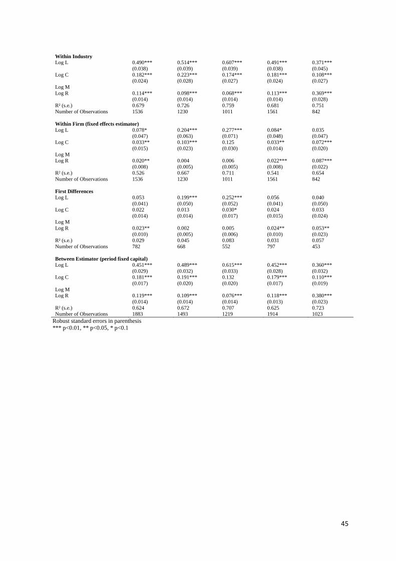
45
Within Industry
Log L 0.490*** 0.514*** 0.607*** 0.491*** 0.371*** (0.038) (0.039) (0.039) (0.038) (0.045)
Log C 0.182*** 0.223*** 0.174*** 0.181*** 0.108*** (0.024) (0.028) (0.027) (0.024) (0.027)
Log M
Log R 0.114*** 0.098*** 0.068*** 0.113*** 0.369*** (0.014) (0.014) (0.014) (0.014) (0.028)
R² (s.e.) 0.679 0.726 0.759 0.681 0.751
Number of Observations 1536 1230 1011 1561 842
Within Firm (fixed effects estimator)
Log L 0.078* 0.204*** 0.277*** 0.084* 0.035 (0.047) (0.063) (0.071) (0.048) (0.047)
Log C 0.033** 0.103*** 0.125 0.033** 0.072*** (0.015) (0.023) (0.030) (0.014) (0.020) Log M
Log R 0.020** 0.004 0.006 0.022*** 0.087*** (0.008) (0.005) (0.005) (0.008) (0.022) R² (s.e.) 0.526 0.667 0.711 0.541 0.654
Number of Observations 1536 1230 1011 1561 842
First Differences
Log L 0.053 0.199*** 0.252*** 0.056 0.040 (0.041) (0.050) (0.052) (0.041) (0.050) Log C 0.022 0.013 0.030* 0.024 0.033 (0.014) (0.014) (0.017) (0.015) (0.024) Log M
Log R 0.023** 0.002 0.005 0.024** 0.053** (0.010) (0.005) (0.006) (0.010) (0.023) R² (s.e.) 0.029 0.045 0.083 0.031 0.057
Number of Observations 782 668 552 797 453
Between Estimator (period fixed capital)
Log L 0.451*** 0.489*** 0.615*** 0.452*** 0.360*** (0.029) (0.032) (0.033) (0.028) (0.032)
Log C 0.181*** 0.191*** 0.132 0.179*** 0.110*** (0.017) (0.020) (0.020) (0.017) (0.019)
Log M
Log R 0.119*** 0.109*** 0.076*** 0.118*** 0.380*** (0.014) (0.014) (0.014) (0.013) (0.023)
R² (s.e.) 0.624 0.672 0.707 0.625 0.723 Number of Observations 1883 1493 1219 1914 1023
Robust standard errors in parenthesis
*** p<0.01, ** p<0.05, * p<0.1

46