initial margin policy and stochastic volatility in the ... margin policy and stochastic volatility...

Initial Margin Policy andStochastic Volatility in theCrude Oil Futures Market

Theodore E. DayUniversity of Texas at Dallas

Craig M. LewisVanderbilt University

This article examines the relationship betweenthe volatility of the crude oil futures market andchanges in initial margin requirements. Toclosely match changes in futures market volatil-ity with the corresponding changes in marginrequirements, we infer the volatility of the fu-tures market from the prices of crude oil futuresoptions contracts. Using a mean-reverting diffu-sion process for volatility, we show that changesin margin policy do not affect subsequent marketvolatility.

Dramatic short-run increases in the volatility of finan-cial markets such as the extraordinary volatility fol-lowing the stock market decline in October 1987 haverenewed interest in the relation between initial mar-gin requirements and market volatility. Hardouvelis(1988) argues that there is a significant negative rela-tion between initial margin requirements on stocksand stock market volatility. This contradicts earlier

This article was presented at the Third Annual Winter Finance conference atthe University of Utah, the Fifth Annual Conference of the Financial OptionsResearch Centre at the University of Warwick, and at Vanderbilt University.We would like to thank Kaushik Amin, Cliff Ball, Don Chance, AndrewKarolyi, Andrew Lo (the editor), Raymond Melkomian, Barry Schacter, PaulSeguin, Hans Stoll, an anonymous referee, and conference participants formany helpful comments. This research was supported through the FinancialMarkets Research Center at Vanderbilt University by a grant from the NewYork Mercantile Exchange and by the Dean’s Fund for Faculty Researchat the Owen Graduate School of Management. Address correspondence toTheodore E. Day, School of Management, University of Texas at Dallas,Box 830688, Sta Jo 5.1, Richardson, TX 75083-0688.

The Review of Financial Studies Summer 1997 Vol. 10, No. 2, pp. 303–332c© 1997 The Review of Financial Studies 0893-9454/97/$1.50

The Review of Financial Studies / v 10 n 2 1997

research by Moore (1966) and Officer (1973) which concludes thatmargin requirements have no effect on the volatility of the stock mar-ket. Hsieh and Miller (1990) present evidence suggesting that the re-lation between margin requirements on stock and volatility found byHardouvelis may be spurious since his methodology is biased in favorof finding a statistical relation between margins and volatility. Insteadthey find that the relation between margin changes and stock marketvolatility is consistent with a tendency for the Federal Reserve Boardto increase initial margin requirements as a response to increases inthe volatility of the stock market. This interpretation of the evidenceis consistent with that of Schwert (1988).

Seguin (1990) examines the relation between margin requirementsand volatility by comparing the volatility of NASDAQ securities duringthe periods before and after each stock becomes eligible for margintrading. For each of the stocks that he examines, volatility declines inthe period following the approval of margin trading. Seguin and Jarrell(1993) examine the impact of margin trading on NASDAQ securitiesduring the stock market crash on October 19, 1987. In spite of thefact that marginable securities had greater abnormal volume during thecrash, Seguin and Jarrell (1993) find that the impact of the crash on theprices of marginable securities was no greater than the correspondingimpact on the prices of securities that were not eligible for margintrading.

The debate over the relation between margin policy and the volatil-ity of financial markets extends to the initial margin requirements infutures markets. The margin requirement for stocks is set by the Fed-eral Reserve Board. In contrast, changes in the required margins formost futures contracts are initiated by the futures clearinghouse with-out prior approval from the Commodity Futures Trading Commission.This permits futures margins to be used as an endogenous risk man-agement tool by the clearinghouse [see Fenn and Kupiec (1993) andDay and Lewis (1996)]. The primary difference between initial marginrequirements in the stock and futures markets is that the initial mar-gin requirements in the stock market are set with respect to the ”loanvalue” of the position, whereas initial margins on futures contractsare designed to guarantee that the buyer and seller will be able tofulfill their contractual obligations. For this reason, the initial marginrequirement for stocks is expressed in terms of the percentage of thepurchase price that must be paid in cash, while margin requirementsin futures markets are set by the respective futures exchanges in termsof a fixed dollar amount per contract. These differences have led toa controversy among regulators because futures margins tend to be amuch smaller percentage of the contract value than the current 50%margin required for stocks. In part, the greater leverage available from

304

Crude Oil Futures Initial Margin Policy and Stochastic Volatility

trading in stock index futures has been blamed by some for the ex-cessive stock market volatility during October 1987. This has led toa number of proposals to consolidate the authority to regulate mar-gins in both the stock and futures markets with the Federal ReserveBoard. Such a change in the regulation of margin requirements wouldsupposedly allow regulators to control the volatility of the marketsthrough both the equalization of the leverage available in the stockand futures markets and through increases of initial margins to moreprudent levels at the appropriate times.

The impact of margin requirements on the volatility of futures mar-kets has been examined by Kupiec (1989) and Kupiec and Sharpe(1990). Kupiec and Sharpe model the effect of margin requirements onportfolio choice in an economy with heterogeneous investors. Theiranalysis shows that margin requirements may either increase or de-crease the volatility of prices according to the nature of the hetero-geneity across investors. Kupiec examines the relation between stockmarket volatility and the margin requirements for S&P 500 futurescontracts and finds that high margin rates in the futures market tendto be associated with above average volatility in the (cash) market forthe S&P 500 stocks. The relation between margin requirements andfutures market volatility has been examined by Fishe et al. (1990) fora sample of 10 futures contracts on agricultural commodities and pre-cious metals. As was the case in Kupiec, they find no evidence of astatistical relation between margin requirements and the subsequentvolatility of the futures market.

A change in margin requirements following a perceived change inthe volatility of a given market is usually implemented quickly, of-ten within the same trading session in futures markets. However, theneed to use a time series of daily returns to estimate the volatility ofthe market has forced most previous research to examine the rela-tion between volatility and margin requirements over relatively longtime intervals [e.g., Hsieh and Miller (1990) use a monthly time in-terval]. In highly volatile markets, this can obscure the true relationbetween margin requirements and volatility. Although this problemcan be circumvented by using transactions data to focus on the intra-day volatility of the market in question, the approach taken here is toinfer both the spot volatility and the parameters of a mean-revertingdiffusion process for volatility from the prices of call options on futurescontracts. The joint estimation of the spot volatility and the stochas-tic process for volatility has several advantages. First, since optionprices should respond instantaneously to changes in volatility, infer-ring volatility from option prices permits us to closely match changesin the volatility of the futures market with both the correspondingchanges in margin requirements and with any feedback effects on

305


volatility from the change in margin requirements. Further, to the ex-tent that increases in the volatility of a particular market are transitoryor mean reverting, the parameters of the stochastic process can pro-vide an estimate of the time required for the volatility of the marketto return to more normal levels.

This article extends previous research by examining the relationbetween changes in margin requirements and changes in consensusforecasts of the volatility of the crude oil futures market. This marketis unique with respect to the frequency with which the New YorkMercantile Exchange adjusts the initial margin requirements for themost actively traded futures contracts (the nearest to delivery or spotmonth contract). Since the beginning of trading in options on crudeoil futures in late 1986, there have been 30 changes in the initial mar-gin requirements for the spot month futures contract. In contrast, themargin requirement for stocks has been changed only 19 times since1945 and has been constant at the current level of 50% since 1974.Consequently the market for crude oil futures provides a unique op-portunity to study the behavior of ex ante forecasts of futures marketvolatility during the time interval surrounding changes in initial marginrequirements.

The focus of our analysis on the interaction between changes ininitial margin requirements and the ex ante volatility of the futuresmarkets represents a departure from previous work, which focuseson the relation between margin requirements and realized volatil-ity. Building on the work of Ball and Roma (1994), Heston (1993),Hull and White (1987), Johnson and Shanno (1987), Stein and Stein(1992), and Wiggins (1987), we examine the impact of changes in ini-tial margin policy on ex ante volatility within an asset pricing frame-work that permits volatility to be stochastic. Given the assumptionthat the prices of futures options accurately reflect a consensus fore-cast of future volatility, generalized method of moments estimationcan be used to obtain estimates of the short-run or spot volatility ofthe futures market. This procedure also provides estimates of the pa-rameters of the diffusion process for the volatility of the crude oilfutures market. The impact of changes in initial margin requirementson ex ante volatility can be examined by using these parameter esti-mates and the implied spot volatility of the crude oil futures marketto create a time series of consensus forecasts of future volatility. Sinceimplied stochastic volatilities from the options market reflect the ex-pectations of market participants concerning the potential range of fu-ture price movements, the stochastic volatilities implicit in the pricesof crude oil futures options provide new evidence concerning theeffect of changes in margin requirements on the volatility of futuresmarkets.

306


This article is organized as follows. Section 1 describes the estima-tion of risk in markets with stochastic volatility and characterizes theasset pricing framework. In Section 2 we discuss the estimation of thestochastic volatility model from the prices of call options on crude oilfutures contracts using generalized method of moments. Section 3 de-scribes the data. The estimated parameters of the mean-reverting pro-cess for stochastic volatility are discussed in Section 4. The behavior offorecasts of forward volatility from the options market during the pe-riod surrounding changes in initial margin requirements is examinedin Section 5. Section 6 examines the causal relation between mar-gin requirements and futures market volatility using Granger causalitytests [see Granger (1969)]. Section 7 concludes the article.

1. The Estimation of Risk in Markets with Stochastic Volatility

Many stochastic volatility models have been proposed in the litera-ture. In this article we assume that the variance of crude oil futuresfollows a square-root diffusion process. The mean-reverting natureof this process is attractive for several reasons. First, Day and Lewis(1993) show that volatility shocks in the crude oil futures market arepersistent and mean reverting. Second, the relation between the spotvolatility and the long-run volatility can be examined directly. Finally,this process is analytically tractable. Cox et al. (1985) implicitly solvefor the moment-generating function of the average of this processin the derivation of their formula for the price of a discount bond.Ball and Roma (1994) use this result to derive a simple closed-formexpression for the expected value of average future volatility. Giventhis result, estimates of the parameters of the diffusion process for fu-tures market volatility can be used to determine the market forecastsof volatility implicit in the prices of call options on crude oil futurescontracts. These parameter estimates also can be used to generate theterm structure of expected average volatility and forward expectedaverage volatilities.

Note that pricing options using the standard techniques for risk-neutral pricing is not possible when volatility is a state variable, sincea perfect hedge for the risk associated with changes in the volatilityof the underlying asset does not exist. Consequently the valuation ofderivative securities is no longer preference free and the market priceof volatility risk, φ(ν), is required to determine the price of an optionon a futures contract.

Assume that the dynamics of the futures price are given by

dF = µF dt +√νF dz1(t), (1)

307


where µ and ν are respectively the instantaneous mean and varianceof the futures price and z1(t) is a standard Wiener process. The in-stantaneous (spot) variance of the futures price is assumed to evolvestochastically according to the diffusion process,

dν = α(β − ν)dt + ζ√ν dz2(t), (2)

where α determines the speed at which the instantaneous variancereverts to its long-run mean β and z2(t) is a standard Wiener processsuch that the instantaneous correlation between increments in z1(t)and z2(t) is ρ.

Let the price of a call option on a futures contract be denoted byC . Given that the cost of carrying a futures contract is zero, the partialdifferential equation that must be satisfied by the price of a futuresoption is

∂C

∂t+ 1

2νF 2 ∂

2C

∂F 2+ ρνζF

∂2C

∂F ∂ν+ 1

2ζ 2ν

∂2C

∂ν2

+ (α(β − ν)− φν)∂C

∂ν− rC = 0. (3)

This differential equation can be solved to obtain the price of anoption on a futures contract by applying the appropriate boundaryconditions and specifying φ. Note that since crude oil futures contractsare American options, the boundary conditions must incorporate thepossibility of early exercise at each moment prior to expiration. Sincethere is no analytic solution for this problem, Equation (3) is solvednumerically.1

The solution to the partial differential equation is a function ofthe spot volatility (a state variable) and five parameters that definethe bivariate system of stochastic differential equations specified byEquations (1) and (2), that is, C = C (ν, α, β, ζ, ρ, φ). Equation (3)shows that there is a linear relation among α, β, and φ that doesnot permit their unique identification. Because the market price of

1 We use finite difference methods to estimate the value of call options on crude oil futures contracts.The computation of a numerical solution to a partial differential equation of the type representedby Equation (4) is complicated by the fact that the partial differential equation includes a mixedpartial derivative. For partial differential equations having mixed derivatives, Gourlay and McKee(1977) show that the “line hopscotch” approach developed in Gourlay (1970) provides moreaccurate solutions than do techniques such as “ordered odd-even” hopscotch, alternating directionimplicit, and local one dimensional methods. This technique, which we use to compute call optionprices, has previously been used by Kuwahara and Marsh (1992) and Wiggins (1987) to priceoptions on financial instruments having a stochastic volatility. The partial differential equation issolved after transforming the variables to make the price of an option a function of the naturallogarithm of the futures price (ln F ) and the natural logarithm of the spot volatility (ln ν).

308


risk, φ, cannot be separated from the terms that govern the drift ofthe volatility diffusion, we estimate a “risk-neutralized” version of thepartial differential equation given by Equation (3). That is,

∂C

∂t+ 1

2νF 2 ∂

2C

∂F 2+ ρνζF

∂2C

∂F ∂ν+ 1

2ζ 2ν

∂2C

∂ν2

+ α∗(β∗ − ν)∂C

∂ν− rC = 0. (4)

Under this specification [see Heston (1993)], the instantaneous vari-ance of the futures price follows the “risk-neutralized” square rootdiffusion

dν = α∗(β∗ − ν)dt + ζ√ν dz2(t), (5)

where α∗ = α + φ and β∗ = αβ/(α + φ). Although the long-runmean volatility and the speed of reversion to the mean cannot beseparately identified using the parameters of the risk-neutral diffusionimplicit in the prices of futures options, the risk-neutral partial differ-ential equation [Equation (4)] can be used to exactly determine theimplied value for the spot volatility of the futures price. In the next sec-tion we discuss the statistical procedures that are used to jointly esti-mate the spot volatility and the parameters of the risk-neutral diffusionprocess.

2. Parameter Estimation of the Stochastic Volatility Model

The parameters of the stochastic volatility model and the spot volatilityof the crude oil futures are estimated using Hansen’s (1982) general-ized methods of moments (GMM). Conceptually our implementationof this procedure is similar to the estimation of an implied volatil-ity using the Black–Scholes model. However, under the assumptionthat volatility is stochastic, the price of the call option is a nonlinearfunction of the spot volatility, ν, and four parameters—α∗, β∗, ζ , andρ—that are assumed to be constant over the sample period. Since theprice of each call option must be calculated numerically, estimationof the underlying parameters is computationally intensive. To easethe burden of computation, we implement a two-stage estimation ap-proach. In the first stage, a subset of the data is used to estimate2p = (α∗, β∗, ζ, ρ) along with the spot volatility for each of the daysincluded in the first-stage estimation sample. This produces a param-eter vector Θ = (2p,3), where Λ is a vector of spot volatilities foreach day in the estimation sample, Λ = (ν1, . . . , ν49). In the secondstage, we estimate the spot volatilities for the remaining days in the

309


sample under the constraint that the parameter vector Θp equals theestimate obtained in the first-stage of the procedure.2

2.1 First-stage estimationTo ensure that the dynamics of the volatility during the sample periodare accurately captured by the diffusion parameters that we estimate,the subset of data that is used in the first stage of the estimation processspans the entire sample period. This subset is created by selecting theat-the-money option for each expiration series on every 20th day ofthe sample, resulting in a sample of 121 observations from 49 differentdays.3

The first-stage estimate of the parameter vector, Θ, is determinedusing the vector of sample moments,

gT (2) = 1

T

T∑t=1

Nt∑n=1

(Ct (X , τn)− C (X , τn,2))Ztn,

where Ct (X , τn) is the date t market price of the at-the-money calloption with strike price X and time to expiration τn, C (X , τn,2) isthe model price at time t , Ztn is the vector of partial derivatives ofC (X , τn,2) with respect to the parameter vector (Θ) weighted by theproportion of the day t trading volume in option n, T is the totalnumber of days in the first-stage estimation sample (T = 49), Nt isthe number of expiration series trading on day t , and T is the totalnumber of observations (T = 121).4 The estimation of 2 using theGMM procedure requires the minimization of the quadratic form,

JT (2) = gT (2)′Ä−1

T gT (2), (6)

where

ÄT = E [((Ct (X , τn)−C (X , τn,2))Ztn)((Ct (X , τn)−C (X , τn,2))Ztn)′].

2 Our sample includes every option that has at least 7 days to expiration and trading volume ofat least 100 contracts during the day. The requirement that trading volume exceed 100 contractseliminates thinly traded contracts, for which the closing trade in the option is very likely to occurprior to the closing trade in the underlying futures contract. By using only options having at least7 days to expiration, we eliminate options for which the option premium is too small to providea precise estimate of the implied volatility of the futures market.

3 The first-stage sample is restricted to the at-the-money option for each expiration series in orderto reduce the computational burden required to estimate the parameters of the stochastic volatilitymodel. Since the at-the-money option is usually the most actively traded contract within a givenexpiration series, using at-the-money options helps to reduce the estimation error arising from alack of simultaneity between the closing futures price and the final price quotation for the calloption.

4 At-the-money options are used because trading volume is concentrated in the at-the-money op-tions. This further mitigates problems associated with nonsynchronous price data. At-the-moneyoptions also are the most sensitive to changes in volatility.

310


Hansen (1982) demonstrates that the asymptotic distribution of theGMM estimator is√

T (2T −20)a∼ N (0, (DtÄ

−1T DT )

−1),

where DT is the Jacobian matrix of gT (2) with respect to 2 evaluatedat 2T .

The specification of the model can be tested using the minimizedvalue of the quadratic form in Equation (6). Under the null hypothesisthat the model is true, this value is asymptotically distributed as χ2

with degrees of freedom equal to T less the number of parameters,that is,5

T gT (2)′Ä−1

T gT (2)a∼ χ2

68.

The estimation is implemented using the standard two-step pro-cedure in Hansen and Singleton (1982). The first step estimates theparameter vector by minimizing Equation (6), with Ä−1

T equal to theidentity matrix. This provides a consistent estimator of the parametervector, which then is used to compute the optimal weighting matrix.The second step reestimates the parameter vector using the optimalweighting matrix.

2.2 Second-stage estimationIn the second stage of the estimation procedure, the daily spot volatil-ities are estimated using the estimate of the parameter vector Θp fromthe first step. Given an initial estimate of the spot volatility, νn

t0, an up-dated estimate, νn

t , is obtained using a Newton–Raphson procedure.At each iteration of the process, the new estimate of νn

t is given by

νnt = νn

t0 + ω(∂C nt /∂ν)

−1εnt ,

where ω is the step size for updating the spot volatility, ∂C nt /∂ν is

the numerical partial derivative of C (X , τn,2p) with respect to thespot volatility evaluated at νn

t0, and εnt is equal to Ct (X , τn) minus

C (X , τn,2p). The estimate of νnt is taken as acceptable when εn

t con-verges to within the desired tolerance level. If the estimate is notwithin the desired tolerance level, the procedure is repeated using νn

tin place of νn

t0.

5 The number of degrees of freedom equals 68, which is determined by the total of the 121 ob-servations less the sum of the number of spot volatility estimates (49) and the parameters of thesquare-root diffusion that are constant over time (4).

311


3. Data Description

The data consist of daily closing prices for call options on crude oilfutures and the underlying futures contracts from the beginning oftrading in the options on November 14, 1986, through March 18, 1991.The risk-free rate of interest for each option expiration series is com-puted for each day using the average of the bid and ask discounts forthe U.S. Treasury bill whose maturity is closest to the expiration date.Bid and ask discounts for U.S. Treasury bills are collected daily fromthe Wall Street Journal.

The New York Mercantile Exchange supplied the dates and marginlevels for all adjustments of initial margin requirements in the nearbyfutures contract (the spot month futures contract). While there werea small number of changes in margin requirements prior to the in-ception of trading in futures options, most of the changes in marginrequirements have occurred since 1986. This period is of particularinterest since it includes the August 1, 1990, invasion of Kuwait byIraq. The sample includes 19 changes in margin requirements priorto the invasion of Kuwait and 11 changes in margin requirements inthe subsequent period.

4. Estimation Results

This section presents estimates of the parameters that describe theevolution of the spot volatility of the crude oil futures market. Inaddition, we present summary statistics for the implied spot volatilitiesderived from these parameter estimates.

4.1 Parameter estimates of the “risk-neutralized” stochasticvolatility model

The first stage of the GMM procedure outlined in Section 3 providesestimates of the parameters of the risk-neutralized diffusion. The pa-rameter estimates of the risk-neutralized diffusion for the volatility ofcrude oil futures, along with their heteroskedasticity-consistent stan-dard errors, are presented in Table 1. With the exception of the es-timate for the correlation between the stochastic component of thefutures price and volatility, the estimated parameters for the modelare all more than three standard errors from zero. The χ2 value of0.00035, corresponding to a p-value less than 0.0001, indicates thatthe model fits the observed option prices quite well.

Table 1 shows that the risk-adjusted long-run mean for the volatilityof the crude oil futures market (β∗) has an estimated value of 0.0718,which corresponds to an annualized standard deviation of approxi-mately 26.8%. Although this represents a lower bound for the long-run

312


Table 1Parameter estimates for the risk-neutralizedstochastic volatility model

Parameter Estimated value t -statistic

α∗ 2.18053 6.075β∗ 0.07183 4.820ζ 0.42932 30.531ρ −0.15684 −0.362

χ 2 value 0.003529Degrees of freedom 68

The parameter estimates for the risk-neutral stochasticvolatility model are obtained from the first stage of theGMM procedure outlined in Section 2. The parameterswere estimated using a subset of the data that includedthe at-the-money options of each expiration series forevery 20th day during the sample period. t -statistics arecomputed using heteroskedasticity-consistent standarderrors.

mean of the true stochastic process, this estimate is reasonable giventhe volatility that has been typical of the crude oil futures markets inrecent years. The estimated value of the mean-reversion parameter(α∗) has an estimated value of 2.181, with a t -statistic of 6.08. Thestandard error of the estimate for α∗ indicates that there is significantmean-reversion in the volatility of the crude oil futures market. Theestimated value for the parameter that determines the time-varyingstandard deviation of the square-root diffusion (ζ ) is 0.429. Given thedynamics for the spot volatility of the futures price, this implies thatwhen the spot volatility is at the long-run mean (of the risk-neutraldistribution), the standard deviation of the spot volatility is 11.5%.Although the estimated value for ρ is −0.157, the standard error ofthe estimate is 0.433, which indicates that the correlation betweenthe futures price and random changes in volatility is not statisticallysignificant.

4.2 Sample estimates of the implied spot volatilitiesTable 2 presents summary statistics for the daily estimates of the spotvolatility for the crude oil futures market. Each of the daily estimateswithin this series represents a weighted average of the implied spotvolatilities for the three futures options nearest to expiration, wherethe weights are based on the numerical partial derivatives of the callprice with respect to spot volatility (normalized to sum to one). Thetime series of implied spot volatilities has a mean value of 0.1704 anda median value of 0.0811. These mean and median values of the spotvariance respectively correspond to annualized standard deviationsof 41.28% and 28.48%. Table 2 indicates that the distribution of theestimates of spot volatility is highly skewed and has fat tails. This isattributable to several dramatic increases in the volatility of the crude

313


Table 2Summary data for estimates of spotvolatility from crude oil futures call optionsfor the period November 14, 1986, to March18, 1991

Statistic Estimated value

Mean 0.1704Median 0.0811Standard error 0.2980Minimum value 0.0117Maximum value 3.1925Skewness 5.01Kurtosis 34.17

The sample period includes 1086 trading days.

oil futures market during the sample period. For example, during theperiod following the invasion of Kuwait by Iraq, the increase in thevolatility of the crude oil futures is both more dramatic and moreprolonged than the volatility observed during the period followingthe stock market crash of 1987.

The first-order autocorrelation of the daily spot volatility series is0.95. This autocorrelation reflects the persistence in volatility that hasbeen characterized by ARCH-type models of conditional volatility. Fig-ure 1 illustrates that the autocorrelation is quite high even at longerlags. The autocorrelation structure of the first differences is also pre-sented in Figure 1. Although the results are not reported, Dickey–Fuller tests reject the possibility of a unit root in favor of the alternativehypothesis that the time series of estimated spot volatilities representsa stationary time series.6

4.3 The parameter estimates of the “true” stochastic volatilitymodel

It is important to note that since the elastic force and long-run mean(α∗ and β∗) of the risk-neutral diffusion given by Equation (6) are func-tions of the parameters of the true stochastic process (of α, β, and φ),the risk-neutral stochastic process must be consistent with the truesample path of the volatility of the crude oil futures market. Therefore,given the functional forms for α∗ and β∗, the parameters of the truestochastic process for volatility can be identified from the parametersof the risk-neutral process if an independent estimate of one of thetrue diffusion parameters can be made. Since the mean-reverting dif-

6 To account for the possibility that misspecification of the time-series process for volatility causesthe results of our statistical tests to be spurious, the stationarity of the spot volatility process isexamined for autoregressive processes having up to 40 lags. At the 1% significance level, everytest rejects the null hypothesis of a unit root in favor of the alternative hypothesis of stationarity.Similar results have been noted by Diz and Finucane (1992), Flemming (1993), and Stein (1989)for implied volatilities from stock index options.

314


Figure 1Autocorrelation functionsThis figure presents the autocorrelation structure of the levels and the first differences of dailyimplied crude oil futures options spot volatilities.

fusion for the spot volatility given by Equation (2) has a steady-statedistribution that asymptotically approaches a gamma distribution witha mean of β, it is tempting to estimate the long-run average volatilityusing the sample average for the implied spot volatilities. However,the extreme volatility of the futures market following the invasion ofKuwait suggests that the sample average of 0.1704 may overstate thetrue long-run volatility. To compensate for the disproportionate num-ber of extreme observations included among our sample estimates, weuse the sample median of 0.0811. This estimate is close to the sampleaverage for the preinvasion period, which is equal to 0.0827. Note thatour estimate of the long-run average volatility is consistent with therequirement that the long-run mean of the risk-neutral distribution beless than the long-run mean of the true distribution.

Given our independent estimate of the long-run mean for the trueprocess for volatility, the risk-neutral estimates of α∗ and β∗ can beused to derive estimates of both the rate of mean reversion for the truevolatility process and the market’s required compensation per unit of

315


volatility risk. The resulting parameter estimates for Equation (2) are

dν = 1.931(0.0811− ν)dt + 0.429√ν dz2(t),

where the elastic force that causes the spot volatility to revert to thelong-run mean, α, has an estimated value of 1.931.7

To provide some indication of the speed at which the estimatedmean-reversion parameter causes volatility to revert to the long-runmean, we use the estimated value for α to infer the spot volatility’s“half-life.” The half-life is defined as the time required for the expectedfuture spot volatility to revert halfway to the long-run mean. The half-life is determined by finding the date, ts , for which

E (νts |νt ) = 1

2(νt + β). (7)

Following Cox, Ingersoll, and Ross (1985), the estimate for the ex-pected future spot volatility is given by

E (νts |νt ) = νt e−α(ts−t) + β(1− e−α(ts−t)). (8)

Examination of Equations (7) and (8) indicates that the half-life isdetermined by setting e−ατ equal to one-half and solving for τ . Givenan estimate for α of 1.931, the expected time for an arbitrary volatilityof ν to revert halfway to its long-run mean is 90 trading days.

The estimate of α for the true stochastic process can be used tocheck the adequacy of our specification for the dynamics of the volatil-ity of the crude oil futures market. Since the theoretical first-order au-tocorrelation for the mean-reverting diffusion given by Equation (2)is e−αdt , the first-order autocorrelation for the time series of impliedspot volatilities can be checked against the theoretical autocorrela-tion based on the estimated value of α. Given that our estimate forα is 1.931, the theoretical first-order autocorrelation in the daily se-ries of implied spot volatilities (based on 250 trading days per year)is 0.9923. As noted previously, the estimate for the autocorrelationof the daily series of implied volatilities is 0.95, with an approximatestandard error of 0.05. Since the implied spot volatilities measure thetrue spot volatility of the futures market with error, this estimate of thefirst-order autocorrelation is a downward-biased estimate of the au-tocorrelation in the true process. Therefore it is not surprising to findthat the estimated first-order autocorrelation is somewhat less than thetheoretical autocorrelation based on the parameter estimate of α. Inspite of this bias, the first-order autocorrelation observed in the im-

7 Cox et al. (1985) demonstrate that if 2αβ/ζ 2 > 1, the drift rate is high enough to prevent nonpos-itive spot volatilities. This condition is satisfied for our parameter estimates (2αβ/ζ 2 = 1.702).

316


plied volatility series is remarkably consistent with the autocorrelationimplied by the estimate for the elastic force of the mean-reverting dif-fusion process, suggesting that the mean-reverting diffusion processfits the data reasonably well.

Since the risk associated with the changing volatility of the futuresmarket cannot be diversified away, the market price of risk, φ, is re-quired to value options on crude oil futures contracts. The estimate forthe market price of risk is 0.25, which enters Equation (3) through theterm φν, a measure of the total compensation for the risk attributableto stochastic volatility. To illustrate the importance of volatility riskto the required returns on a futures contract, suppose that the spotvolatility of the futures market is equal to the long-run mean of 0.0811.For this case the risk premium associated with volatility risk is 0.25 ×0.0811, which represents a risk premium of approximately 2.0% peryear. Since the average annual returns in the futures and stock mar-kets are similar [e.g., Bodie and Rosansky (1980)], a reasonable guessfor the size of the average risk premium would be about 8%. There-fore the compensation for volatility risk appears to be a significantcomponent of the risk premia in the futures market.

4.4 Expected average volatilities and forward volatilitiesFollowing Hull and White (1987) and Merton (1973) it has been com-mon to interpret the implied volatility from the Black–Scholes priceof a call option as the expected average of the spot volatility of theunderlying security over the time remaining until the expiration of theoption.8 We depart from this tradition in that we use the estimated pa-rameters for the mean-reverting diffusion of the volatility for the crudeoil futures market to directly compute estimates of the expected aver-age volatility. Note that while implied volatilities from static volatilitymodels are limited to providing forecasts of the volatility over theremaining life of the option, the estimated parameters from the dy-namic model permit us to derive forecasts of volatility over arbitraryfuture time periods. This feature of the stochastic volatility frameworkpermits greater flexibility in designing empirical tests than is possibleusing traditional methods for inferring volatility from static volatilityoption pricing models.

8 Hull and White (1987) and Merton (1973) discuss the conditions under which the implied volatilityfrom the price of a call option can be interpreted as the expected average of the spot volatilityof the underlying security over the remaining life of the option. While Merton examines thecase where the spot volatility may be at most a known function of time, Hull and White permitvolatility to follow a mean-reverting diffusion process similar to Equation (2). When volatilityfollows a mean-reverting diffusion, Hull and White show that this interpretation of the impliedvolatility is correct only when (1) volatility and price shocks are uncorrelated and (2) the marketrequires no compensation for volatility risk.

317


Ball and Roma (1994) show that the current spot volatility (ν0) canbe used to estimate the expected average volatility over the next τperiods using the formula

E

(1

τ

∫ τ

0νt dt

)= ω(τ)ν0 + (1− ω(τ))β, (9)

where

ω(τ) = eατ − 1

ατeατ.

Equation (9) shows that the expected average volatility is a weightedaverage of the current spot volatility and the long-run mean volatilityof the futures market. It is easy to show that as the length of theforecast horizon (τ ) increases, the weight on the current spot volatilitydecreases, reflecting the tendency for the spot volatility to revert to itslong-run mean of β.

Given our estimates of α and β, Equation (9) is used to transformeach of our daily estimates of the spot volatility into a series of fore-casts of the expected average volatility over forecast horizons rangingup to 2 years. The time series of term structures for the expected aver-age volatility of the crude oil futures market is presented in Figure 2,which presents plots of these term structures for both the period priorto the invasion of Kuwait (panel A) and the period immediately fol-lowing the invasion (panel B). The term structure plots in Figure 2illustrate the mean-reverting nature of the volatility of the crude oilfutures market. For example, note that during the preinvasion periodshown in panel A both upward and downward sloping term structuresare evident, reflecting the tendency for the spot volatility to fluctuatearound its long-run mean during this subperiod. In contrast, panel Bshows that the period following the invasion of Kuwait is character-ized by downward sloping term structures, consistent with the factthat spot volatility remained well-above the long-run mean during theentire postinvasion period.

The term structure of expected average volatilities obtained fromEquation (7) can be used to construct forecasts of future volatility sim-ilar to the forward rates implicit in the term structure of interest rates.Given the estimates for the long-run mean volatility and the currentspot volatility, the expected average volatility over a distant forecasthorizon (having a length of τ2) can be expressed as a weighted av-erage of the expected average volatility over the near-term forecasthorizon (having a length of τ1) plus a forecast of the expected av-erage volatility for a time interval beginning τ1 periods in the futureand having a length of τ2 − τ1. By comparing the expected averagevolatilities for two forecast periods ending respectively in τ1 and τ2

318


Figure 2Expected average colatilities from crude oil futures optionsThis figure plots the term structure of expected average volatilities from crude oil futures options.The top and bottom figures illustrate a time period immediately preceding the invasion periodand the invasion period, respectively.

319


periods, the forward volatility for the period beginning at τ1 can beexpressed as

E

((1

τ2 − τ1

)∫ τ2

τ1

νt dt

)= β + 1

τ2 − τ1 (ν0 − β)eατ2 − eατ1

αeα(τ2+τ1). (10)

The forward volatilities defined by Equation (10) are particularly use-ful in examining the relation between changes in margin requirementsand volatility because they provide an ex ante forecast of future volatil-ity that reflects the anticipated decay of shocks to short-run volatilitythat are coincident to changes in margin requirements.

5. Empirical Tests of the Relation Between Margin Requirementsand Volatility

The empirical tests that we use are designed to distinguish betweentwo alternative hypotheses concerning the impact of margin require-ments on the volatility of futures markets. According to the first hy-pothesis, the required margin on a futures contract is a control variablethat can be used to dampen excessive volatility. Alternatively, as ar-gued by Day and Lewis (1996) and Fenn and Kupiec (1993), changesin margin requirements are used as a risk management tool by thefutures clearinghouse to control for the impact of volatility on thecounterparty risk implicit in futures trading. Each of these hypothe-ses suggests that increases (decreases) in margin requirements shouldtend to occur following increases (decreases) in volatility. However,under the first hypothesis, the increase (decrease) in margin require-ments should reduce (increase) volatility in the period subsequent tothe change in margin requirements, while under the second hypothe-sis the volatility of the return-generating process may be independentof the prevailing margin requirement.

To distinguish between these alternative hypotheses, we examinethe changes in the forward volatility of the crude oil futures marketduring an event window beginning 10 days prior to a change in mar-gin requirements and ending 10 days following the change in marginrequirements. If increases in initial margin requirements cause thevolatility of the futures market to decline, we should expect to seethe forward volatility fall to a lower level during the 10-day periodfollowing the implementation of an increase in the initial margin re-quirement. However, since the volatility of the crude oil futures marketfollows a mean-reverting stochastic process, a decrease in volatility isconsistent with the hypothesis that the volatility of the futures marketis independent of margin requirements so long as increases in initial

320


margin requirements tend to follow increases in volatility. Similar logicapplies to decreases in margin requirements.

To test the hypothesis that changes in margin requirements havea causative effect on volatility against the null hypothesis that thefutures clearinghouse changes margin requirements to control for in-creases in counterparty risk, we compare futures market volatility foreach day in the event window to the volatility 10 days prior to thechange in margin requirements. These comparisons allow us to estab-lish whether changes in margin requirements represent a response tochanges in expected volatility. They also provide a statistical compar-ison of volatility before and after changes in margin requirements. Todistinguish between margin effects and the impact of mean-reversionin the period subsequent to a change in margin requirements, we thencompare the spot volatility for each day following a change in marginrequirements with the spot volatility that would have been expectedgiven the volatility on the day of the change in margin requirements.

Note that whereas previous research examines the (ex post) vari-ance of returns in the time periods preceding and subsequent tochanges in margin requirements, our estimates of the forward volatil-ity of the crude oil futures market represent ex ante forecasts of thefuture volatility implicit in the prices of futures call options. The useof an ex ante estimate of the volatility allows the forward volatili-ties to be interpreted in terms of changes in investors’ perceptionsconcerning the future volatility of the crude oil futures market. Whileidentical results are obtained from comparisons based solely on spotvolatilities, the forward volatilities illustrate the impact of the volatilityshocks during the event window on the anticipated future volatilityof the crude oil futures market.

5.1 Formulation of the null hypothesisTo test the significance of changes in volatility during the periodsboth prior to and subsequent to the change in margin requirements,we examine changes in the forward volatility of the crude oil futuresmarket during a 21-day event window beginning 10 days prior toa change in margin requirements and ending 10 days following thechange. Each change in the forward volatility is measured relative tothe forward volatility at the beginning of the event window (day −10).For consistency, the forward volatilities for each day within the eventwindow represent a future 3-month period that is fixed in relation tothe first day in the event window.9

9 Since the beginning of the time period over which the forward volatility is defined can be heldfixed during the (event) window of time surrounding changes in margin requirements, the forwardvolatility provides a useful benchmark against which to measure the impact of both exogenous

321


Under the null hypothesis that there is no change in volatility dur-ing the event window surrounding a change in margin requirements,we should be unable to find any systematic differences in the forwardvolatilities during the period prior to or subsequent to changes in ini-tial margin requirements. Therefore, if we measure changes in forwardvolatility relative to the average forward volatility at the beginning ofthe event window (day t∗), the null hypothesis can be stated as

H0: σ2f t (t1, t2) = σ 2

f t · (t1, t2),

where σ 2f t · (t1, t2) is the forward volatility for some day t within the

event window, and t2 − t1 is always a future time interval havinga length of 3 months. For example, if t1 is 6 months from day t∗(t1 = t∗ + 0.50), t2 is 9 months from day t∗ (t2 = t∗ + 0.75). Note thatfor increases in margin requirements, we would expect the forwardvolatility for the futures market to increase from the beginning of theevent window until the date that the initial margin requirement is in-creased and then either decrease or remain unchanged depending onthe impact of the change in initial margin requirement. Therefore, forincreases in the margin requirements, the alternative hypothesis is thatthe difference in the forward volatilities should be significantly greaterthan zero. Conversely, for decreases in margin requirements, the al-ternative hypothesis is that the difference in the forward volatilities issignificantly less than zero.

We test for the significance of changes in our forecasts of futurevolatility using two different approaches. First, we perform t -tests forthe significance of the average changes in volatilities using an ap-proach similar to Day and Lewis (1988). Since it is possible that themeasurement errors associated with the implied spot volatility are het-eroskedastic, we also test the null hypothesis using two nonparametricprocedures: the Wilcoxon signed-rank test10 and the Mann–Whitneyrank test.11 Because the forward volatilities are monotone transfor-

changes in the spot volatility and any corresponding changes in margin requirements.10 For increases in margin requirements, we test the null hypothesis that there is no significant

increase in volatility in either the 10 days prior to or the 10 days following an increase in themargin requirements. Therefore, the Wilcoxon signed-rank test statistic is calculated using the sumof the ranks of the negative differences in the forward volatilities form day t∗ to t , which shouldbe less than the sum of the ranks of the positive differences under the alternative hypothesis. Thesmaller the sum of the negative ranks, the smaller is the probability of rejecting a null hypothesisthat is true. This logic is reversed in testing the null hypothesis for the subset of decreases ininitial margin requirements.

11 Whereas the Wilcoxon signed-rank statistic is used to test the null hypothesis that the averagedifference in the forward volatilities is equal to zero, the Mann–Whitney rank test considers thenull hypothesis that the forward volatility on day t comes from the same distribution as the forwardvolatility on day t∗. For increases in initial margin requirements, the forward volatility on day twould be greater than the forward volatility on day t∗ under the alternative hypothesis. This ranktest statistic is determined by ranking the forward volatilities and then computing the number of

322


mations of the spot volatility, the test statistics and related p-valuesare the same across different forecasting horizons. Therefore we onlyreport one set of values.

We also examine the impact of changes in margin requirementsby comparing the average spot volatility for each of the 10 eventdays following the change in margin requirements with the averageexpected volatility for that day conditional on the spot volatility atday 0 [see Equation (8)]. Note that the comparison described aboveexplicitly distinguishes between decreases in volatility (relative to day0) that are attributable to the normal expected decay of above averagelevels of volatility and decreases that are attributable to the dampeningeffect of increases in margin requirements.

5.2 Empirical resultsThe extent and magnitude of changes in the volatility of the crude oilfutures market during the periods prior to and subsequent to changesin initial margin requirements provide important evidence concerningthe impact of margin requirements on futures market volatility. In thissection we present evidence that shows that although increases anddecreases in margin requirements are preceded by significant changesin futures market volatility, margin policy has no permanent impacton the volatility of the futures market.

The average changes in forward volatilities relative to the forwardvolatility at the beginning of the 21-day event window surroundingchanges in margin requirements are presented in Table 3. These for-ward volatilities represent forecasts of future volatility for 3-monthperiods that respectively begin 3, 6, 9, and 12 months from the firstday of the event window (day −10). In panel A we report the aver-age changes in forward volatilities in the event window surroundingthe 22 increases in initial margin requirements included in the sample.Note that each of the four forward volatility series reflects a noticeableincrease in volatility on the day prior to the increase in initial marginrequirements (day −1). For example, the average increase in the 3-month forward volatility in the period prior to the margin change is0.0307, which represents an increase of approximately 23% relativeto the forward volatility at the beginning of the event window. Thisincrease is statistically significant for all forecasting periods. Note thatthe average increase in forward volatility decreases as the forecastinghorizon increases. This reflects both the mean-reverting nature of thesquare-root diffusion and the tendency for increases in initial margin

forward volatilities for day t that are exceeded by each of the forward volatilities on day t∗. Thisstatistic should be small under the alternative hypothesis that the forward volatility at day t isgreater than the forward volatility at day t∗.

323


Table 3Average forecasts of volatility during the event window surrounding changes in marginrequirements

Days relative to initial margin changeAverage forwardvolatility estimate −10 −5 −1 0 1 5 10

Panel A: Initial margin increases (n = 22):

3-month forward volatility:Average forward volatility 0.1331 0.1437 0.1639 0.1711 0.1606 0.1735 0.1397Volatility difference 0.0106 0.0307 0.0379 0.0274 0.0404 0.0066




t -statistic 1.07 2.05 1.61 1.69 1.26 0.33Wilcoxon signed-rank test 0.153 0.055 0.143 0.245 0.207 0.863Mann–Whitney rank test 0.789 0.658 0.450 0.545 0.600 0.816

Panel B: Initial margin decreases (n = 8):

3-month forward volatility:Average forward volatility 0.4292 0.2999 0.2824 0.2714 0.2795 0.2747 0.2727Volatility difference −0.1293 −0.1468 −0.1580 −0.1497 −0.1545 −0.1566




t -statistic −1.00 −0.94 −0.99 −0.96 −0.94 −0.88Wilcoxon signed-rank test 0.547 0.461 0.461 0.461 0.547 0.641Mann–Whitney rank test 0.796 0.680 0.538 0.643 0.505 0.505

The average forward volatility for a 3-month period starting n months from the first day (−10)of a 21-day event window is reported for selected days within the event window. These forwardvolatilities, along with the changes relative to the forward volatility at the beginning of theevent window, are reported for 3-month periods beginning 3, 6, 9, and 12 months from day−10. Heteroskedasticty-consistent t -statistics are for the average difference between the forwardvolatilities for day t and day −10. The Wilcoxon signed-rank test reports the p-value for thehypothesis that the day t forward volatility is unaffected by changes in the initial marginrequirements. The Wilcoxon–Mann–Whitney test indicates that the null hypothesis that the forwardvolatilities from day t and day −10 come from the same distribution should not be rejected forany significance level below this value.

requirements to occur when the spot volatility exceeds the long-termvolatility of the futures market.

The increases in forward volatilities observed from day −10 to day0 seem to reverse during the 10-day period following increases in

324


margin requirements. In fact, the results presented in panel A showthat we are unable to reject the null hypothesis that the volatility atthe end of the event window is on average equal to the volatility atthe beginning of the event period. Note that the data fail to reject thisnull hypothesis under both the parametric and nonparametric teststhat we conduct.

The results for the eight decreases in the initial margin require-ments are reported in panel B. Note that the average levels for theforward volatilities are uniformly greater than the corresponding for-ward volatilities reported in panel A. This reflects the fact that sev-eral of the decreases in margin requirements occurred in January andFebruary 1991, when the volatility of the oil futures market was de-clining from unprecedented levels. While it is difficult to make generalclaims about eight observations, it is of interest to note that the forwardvolatilities decline in the week prior to the announcement week (days−10 to −6), but remain essentially unchanged during the remainderof the event period (days −5 to 10).

The results presented in Table 3 are consistent with the argumentthat the clearinghouse increases and decreases initial margin require-ments in response to increases and decreases in the volatility of thefutures market. Panel A shows that increases in forward volatility dur-ing the period prior to the increase in margin requirements seem toreverse themselves in the subsequent 10-day period. A related resultis observed in panel B, where we see that the drop in futures marketvolatility that precedes the reduction in margin requirements does notcontinue into the second half of the event period.

The interpretation of these results is unclear. Since the averagevolatility in the period surrounding an increase in margins is at itshighest on the announcement date, the decrease in average volatilityfollowing the change in margin requirements can be attributed eitherto the effect of the increase in margins or the tendency for transitoryshocks to volatility to decay over time. For decreases in margin re-quirements, we see that the average volatility on the announcementdate is well above the long-run mean of volatility. Therefore, whereasthe volatility of the futures market is relatively constant in the pe-riod following the announcement date, under the null hypothesis thatdecreases in margin requirements have no effect on volatility, thespot volatility would be expected to decay in the period followingdecreases in margin requirements.

To separate the impact of changes in margin requirements frommean-reversion in volatility, we compare the average spot volatilitywith the corresponding average of the expected future spot volatility(conditional on the day 0 spot volatility) for each day in the eventwindow following changes in margin requirements. These results are

325


Table 4Comparison of actual and conditional expected spot volatilities

Increases in margin requirements Decreases in margin requirements

Average Average t -statistic for Average Average t -statistic forspot conditional significance of spot conditional significance of

Day volatility volatility difference volatility volatility difference

1 0.2345 0.2635 −0.27 0.4865 0.4669 0.122 0.3324 0.2621 0.49 0.4680 0.4640 0.033 0.3310 0.2621 0.37 0.4673 0.4610 0.044 0.2792 0.2593 0.17 0.4608 0.4581 0.025 0.2699 0.2580 0.10 0.4767 0.4552 0.126 0.2645 0.2566 0.08 0.4923 0.4523 0.217 0.1842 0.2552 −1.64 0.4955 0.4495 0.248 0.1940 0.2539 −1.25 0.4743 0.4466 0.159 0.1974 0.2526 −1.14 0.4736 0.4438 0.15

10 0.2009 0.2513 −1.07 0.4724 0.4410 0.16

The averages of the spot volatility and the expectation of the spot volatility conditional on volatilityat day 0 are reported for each of the 10 days following a change in margin requirements. To test forsignificance of the differences between the actual spot volatility and the conditional expectation,we report t -statistics computed using the standard deviation of the empirical distribution of actualvolatilities for a given event day. Similar nonparametric results for the Wilcoxon rank-sum test arereported in Section 5.

reported in Table 4. For increases in margin requirements, we findthat although the average spot volatility appears to decline by morethan would be expected given the expected mean-reversion in theannouncement date spot volatility, the difference is not statisticallysignificant for any of the 10 days following the change in marginrequirements. This result is confirmed by performing a two-sampleWilcoxon rank-sum test for the difference between the actual and theconditional expected spot volatility on day 10. The standard normalapproximation for this test statistic has a t -value of −0.49, indicatingthat the actual volatility at the end of the event window is not statisti-cally different than the volatility that would be expected based on themean reversion in the spot volatility observed on the announcementdate. For decreases in margin requirements, the Wilcoxon rank-sumstatistic rejects the null hypothesis that the average spot volatility onday 10 is less than the conditional expected spot volatility. Althoughthe rejection of the null hypothesis implies that decreases in marginrequirements may have slowed the forces causing volatility to decayto its long-run mean, the limited size of the sample suggests that thisresult should be interpreted with caution.

In summary, there is some evidence that ex ante volatility increasestemporarily in the period immediately prior to increases in margin re-quirements. However, we are unable to reject the null hypothesisthat the forward volatilities 10 days prior to changes in margin re-quirements are equal to forward volatilities 10 days after changes inmargins. And while decreases in initial margin requirements are as-sociated with decreases in ex ante volatility, the results suggest that

326


volatility decreases lead (in a statistical sense) decreases in initial mar-gin requirements. Taken together, these results indicate that changesin initial margin requirements have very little short-term impact onthe forecasts of future volatility embedded in the prices of crude oilfutures call options.

6. Tests for Granger Causality

Since the event study approach used in the previous section does notrepresent an explicit test for a causal relation between margin require-ments and futures market volatility, this section provides a formal testof whether initial margin requirements Granger-cause volatility (orvice versa). The causal relation between margin requirements andvolatility is examined using monthly time series for the average initialmargin requirement and the corresponding volatility of the return onthe near-term futures contract. The monthly average initial margin re-quirement is expressed as a fraction of the value of a crude oil futurescontract by dividing the average dollar amount of the initial marginrequirement during the month by the average value of the futurescontract based on the near-term futures price during the month. Weuse two proxies for monthly volatility. The first is the (historic) vari-ance of the return on the near-term futures contract. The second isthe monthly average implied spot volatility. Note that these definitionsof margin requirements and volatility differ from the moving averageproxies used by Hardouvelis (1988) and Hsieh and Miller (1990). Sinceeach of the observations in the time series that we create depend onlyon the events within the month, our results are not affected by theresidual autocorrelation created by using overlapping observations.

Table 5 presents a test of whether initial margin requirementsGranger-cause futures market volatility. The test is implemented byregressing futures market volatility on lagged values of volatility andthe margin requirement for the preceding period. Following Hsieh andMiller (1990), we increase the lags of the dependent variable includedin our regressions until the serial correlation in the regression residu-als has been eliminated. The results presented in Table 5 show verylittle evidence that initial margin requirements Granger-cause eithermeasure of futures market volatility. In each case the coefficient ofthe initial margin requirement fails to be statistically significant, whichimplies that margins do not Granger-cause volatility.

Since the behavior of the implied forward volatilities is consistentwith the hypothesis that margin requirements change in responseto an increase in options market volatility, Table 6 presents testsof whether futures market volatility Granger-causes initial margin re-quirements. For the case where the lagged values of futures market

327


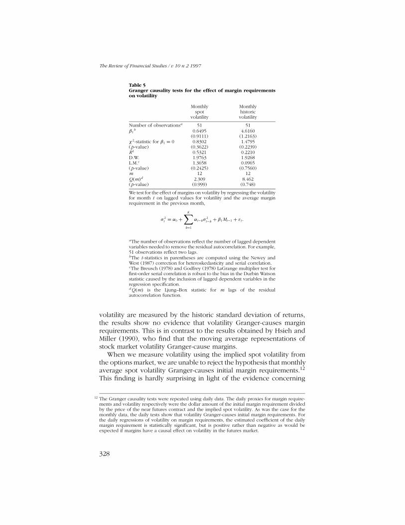
Table 5Granger causality tests for the effect of margin requirementson volatility

Monthly Monthlyspot historic

volatility volatility

Number of observationsa 51 51β1

b 0.6495 4.6160(0.9111) (1.2163)

χ2-statistic for β1 = 0 0.8302 1.4795(p-value) (0.3622) (0.2239)R2 0.5321 0.2210D.W. 1.9763 1.9268L.M.c 1.3658 0.0965(p-value) (0.2425) (0.7560)m 12 12Q(m)d 2.309 8.462(p-value) (0.999) (0.748)

We test for the effect of margins on volatility by regressing the volatilityfor month t on lagged values for volatility and the average marginrequirement in the previous month,

σ 2t = α0 +

K∑k=1

αt−kσ2t−k + β1Mt−1 + εt .

aThe number of observations reflect the number of lagged dependentvariables needed to remove the residual autocorrelation. For example,51 observations reflect two lags.bThe t -statistics in parentheses are computed using the Newey andWest (1987) correction for heteroskedasticity and serial correlation.cThe Breusch (1978) and Godfrey (1978) LaGrange multiplier test forfirst-order serial correlation is robust to the bias in the Durbin Watsonstatistic caused by the inclusion of lagged dependent variables in theregression specification.d Q(m) is the Ljung–Box statistic for m lags of the residualautocorrelation function.

volatility are measured by the historic standard deviation of returns,the results show no evidence that volatility Granger-causes marginrequirements. This is in contrast to the results obtained by Hsieh andMiller (1990), who find that the moving average representations ofstock market volatility Granger-cause margins.

When we measure volatility using the implied spot volatility fromthe options market, we are unable to reject the hypothesis that monthlyaverage spot volatility Granger-causes initial margin requirements.12

This finding is hardly surprising in light of the evidence concerning

12 The Granger causality tests were repeated using daily data. The daily proxies for margin require-ments and volatility respectively were the dollar amount of the initial margin requirement dividedby the price of the near futures contract and the implied spot volatility. As was the case for themonthly data, the daily tests show that volatility Granger-causes initial margin requirements. Forthe daily regressions of volatility on margin requirements, the estimated coefficient of the dailymargin requirement is statistically significant, but is positive rather than negative as would beexpected if margins have a causal effect on volatility in the futures market.

328


Table 6Granger causality tests for the effect of volatility on marginrequirements

Monthly Monthlyspot historic

volatility volatility

Number of observationsa 37 51β1

b 0.1136 -0.0125(6.3752) (-0.4004)

χ2-statistic for β1 = 0 40.6428 0.1603(p-value) (0.0000) (0.6889)R2 0.7721 0.6377D.W. 1.6153 1.9126L.M.c 1.7512 0.0508(p-value) (0.1857) (0.8216)m 9 9Q(m)d 5.256 3.411(p-value) (.811) (0.999)

We test for the effect of volatility on margins by regressing the averagemargin requirement for month t on lagged values of the averagemargin requirement and the volatility from the previous month,

Mt = α0 +K∑

k=1

αt−kMt−k + β1σ2t−1 + εt .

aThe number of observations reflect the number of lagged dependentvariables needed to remove the residual autocorrelation. For example,37 and 51 observations reflect 16 and 2 lags, respectively.bThe t -statistics in parentheses are computed using the Newey andWest (1987) correction for heteroskedasticity and serial correlation.cThe Breusch (1978) and Godfrey (1978) LaGrange multiplier test forfirst-order serial correlation is robust to the bias in the Durbin Watsonstatistic caused by the inclusion of lagged dependent variables in theregression specification.d Q(m) is the Ljung–Box statistic for m lags of the residualautocorrelation function.

the relation between forward volatilities and changes in margin re-quirements presented in Section 5. However, it is interesting to notethat averaging the short-term implied volatilities over a period of 1month fails to attenuate the leading effect of the average increaseof the forward volatilities in the 10-day period preceding increasesin initial margin requirements. The difference in the causality resultsfor the alternative proxies for futures market volatility is most likelyattributable to the speed with which initial margin requirements areadjusted to reflect changes in the uncertainty surrounding the futuresupply and demand for crude oil. Whereas the implied spot volatilitiesfrom the prices of futures options adjust almost immediately to worldevents, the past series of returns tends to contain only limited informa-tion about the causes of short-run changes in market volatility. Giventhat officials at the New York Mercantile Exchange use the impliedvolatility from the options market to monitor volatility of the underly-

329


ing crude oil futures contract, perhaps it should not be surprising thatchanges in margin requirements tend to be caused by changes in theimplied volatility of the futures markets.

7. Conclusion

This article examines the relation between changes in initial margin re-quirements and the volatility of the crude oil futures market. Whereasprevious studies have examined the relation between margin require-ments and ex post volatility of the market in question (e.g., the stockmarket), this article examines the effect of margin requirements onex ante measures of volatility obtained from the prices of crude oilfutures options.

Our study of the behavior of implied stochastic volatilities in theevent window surrounding margin changes provides a number of in-teresting results. As might be expected, we document a tendency forthe ex ante volatility of the crude oil futures market to increase in the10-day period prior to increases in initial margin requirements. How-ever, we find insignificant differences between ex ante volatility 10days prior to an increase in margin requirements and ex ante volatil-ity 10 days after. Although these results are consistent with a numberof hypotheses concerning the relation between volatility and marginrequirements, we perform Granger causality tests that suggest that thechain of causation (in a Granger sense) may run from volatility of thecrude oil futures markets to initial margin requirements.

ReferencesBall, Clifford A., and Antonio Roma, 1994, “Stochastic Volatility Option Pricing,” Journal ofFinancial and Quantitative Analysis, 29, 589–608.

Bodie, Zvi, and Victor Rosansky, 1980, “Risk and Return in Commodity Futures,” FinancialAnalysts Journal, 36, 27–39.

Breusch, T. S., 1978, “Testing for Autocorrelation in Dynamic Linear Models,” AustralianEconomics Papers, 17, 334–355.

Cox, John C., Jonathan E. Ingersoll, Steven A. Ross, 1985, “A Theory of the Term Structure ofInterest Rates,” Econometrica, 53, 385–408.

Day, Theodore E., and Craig M. Lewis, 1988, “The Behavior of the Volatility Implicit in the Pricesof Stock Index Options,” Journal of Financial Economics, 22, 103–122.

Day, Theodore E., and Craig M. Lewis, 1993, “Forecasting Futures Market Volatility UsingAlternative Models of Conditional Volatility,” Journal of Derivatives, 1, 33–50.

Day, Theodore E., and Craig M. Lewis, 1996, “Margin Adequacy in Futures Markets,” unpublishedmanuscript, Vanderbilt University.

Diz, Fernando, and Thomas J. Finucane, 1992, “The Time Series Properties of Implied Volatilityof the S&P 100 Index Options,” unpublished manuscript, Syracuse University.

330


Fenn, George W., and P. Kupiec, 1993, “Prudential Margin Policy in a Futures-Style SettlementSystem,” Journal of Futures Markets, 13, 389–408.

Fishe, Raymond P. H., Lawrence G. Goldberg, Thomas F. Gosnell, and Sujata Sinha, 1990, “MarginRequirements in Futures Markets: Their Relationship to Price Volatility,” Journal of Futures Markets,10, 541–554.

Flemming, Jeff, 1993, “The Quality of Market Volatility Forecasts Implied by S&P 100 Index OptionPrices,” unpublished manuscript, Rice University.

Godfrey, L. G., 1978, “Testing Against General Autoregressive and Moving Average Error Modelswhen the Regressors Include Lagged Dependent Variables,” Econometrica, 46, 1293–1302.

Gourlay, A. R., 1970, “Hopscotch: A Fast Second-Order Partial Differential Equation Solver,”Institute of Mathematics and Applications Journal, 6, 375–390.

Gourlay, A. R., and S. McKee, 1977, “The Construction of Hopscotch Methods for Parabolic andElliptic Equations in Two Space Dimensions with a Mixed Derivative,” Journal of Computationaland Applied Mathematics, 3, 201–206.

Granger, Clive W. J., 1969, “Investigating Causal Relations by Econometric Models and Cross-Spectral Methods,” Econometrica, 37, 424–438.

Hansen, L. P., 1982, “Large Sample Properties of Generalized Method of Moments Estimators,”Econometrica, 50, 1029–1054.

Hansen, L. P., and K. J. Singleton, 1982, “Generalized Instrumental Variables Estimation of Non-Linear Rational Expectations Models,” Econometrica, 50, 1269–1286; errata, 52, 267–268.

Hardouvelis, Gikas, 1988, “Margin Requirements and Stock Market Volatility,” Federal ReserveBank of New York Quarterly Review, Summer, 80–89.

Heston, Steven L., 1993, “A Closed-Form Solution for Options with Stochastic Volatility withApplications to Bond and Currency Options,” Review of Financial Studies, 6, 327–344.

Hsieh, David A., and Merton H. Miller, 1990, “Margin Regulation and Stock Market Volatility,”Journal of Finance, 45, 3–29.

Hull, John, and Alan White, 1987, “The Pricing of Options of Assets with Stochastic Volatilities,”Journal of Finance, 42, 281–300.

Johnson, Herb, and David Shanno, 1987, “Option Pricing when Variance Is Changing,” Journal ofFinancial and Quantitative Analysis, 22, 143–151.

Kupiec, Paul H., 1989, “Futures Margins and Stock Price Volatility: Is There Any Link?,” Journal ofFutures Markets, 13, 677–691.

Kupiec, Paul H., and Steven A. Sharpe, 1990, “Animal Spirits, Margin Requirements, and StockPrice Volatility,” Journal of Finance, 46, 717–731.

Kuwahara, Hiroto, and Terry A. Marsh, 1992, “The Pricing of Japanese Equity Warrants,”Management Science, 38, 1610–1641.

Merton, Robert C., 1973, “The Theory of Rational Option Pricing,” Bell Journal of Economics andManagement Science, 4, 141–183.

Moore, Thomas, 1966, “Stock Market Margin Requirements,” Journal of Political Economy, 74,158–167.

Newey, Whitney K., and Kenneth D. West, 1987, “A Simple, Positive Semi-DefiniteHeteroskedasticity and Autocorrelation Consistent Covariance Matrix, Econometrica, 55, 703–708.

331


Officer, Robert R., 1973, “The Variability of the Market Factor of the New York Stock Exchange,”Journal of Business, 46, 434–453.

Schwert, G. William, 1988, “Business Cycles, Financial Crises and Stock Volatility,” unpublishedmanuscript, University of Rochester.

Seguin, Paul J., 1990, “Stock Volatility and Margin Trading,” Journal of Monetary Economics, 26,101–121.

Seguin, Paul J., and Gregg A. Jarrell, 1993, “The Irrelevance of Margin: Evidence from the Crashof ’87,” Journal of Finance, 48, 1457–1474.

Stein, Elias M., and Jeremy C. Stein, 1991, “Stock Price Distributions with Stochastic Volatility: AnAnalytic Approach,” Review of Financial Studies, 4, 727–752.

Stein, Jeremy C., 1989, “Overreactions in the Options Market,” Journal of Finance, 44, 1011–1023.

Wiggins, James B., 1987, “Option Values under Stochastic Volatility: Theory and EmpiricalEstimates,” Journal of Financial Economics, 19, 351–372.

332

initial margin policy and stochastic volatility in the ... margin policy and stochastic volatility...

Documents