infinitam v3: a framework for large-scale 3d reconstruction ... · infinitam v3: a framework for...
TRANSCRIPT
InfiniTAM v3:A Framework for Large-Scale 3D Reconstruction with Loop Closure
Victor Adrian [email protected]
University of Oxford
Olaf [email protected]
University of Oxford
Stuart [email protected]
University of Oxford
Michael [email protected] Research America
Tommaso [email protected]
University of Oxford
Philip H S [email protected]
University of Oxford
David W [email protected]
University of Oxford
August 3, 2017
Contents
1 Introduction 21.1 What’s New . . . . . . . . . . . . . . . . . . . . . . . . . . . . . . . . . . . . . . . . . . . . 2
2 Cross-Device Implementation Architecture 2
3 Volumetric Representation with Hashes 33.1 The Voxel Block Array . . . . . . . . . . . . . . . . . . . . . . . . . . . . . . . . . . . . . . 33.2 The Hash Table and The Hashing Function . . . . . . . . . . . . . . . . . . . . . . . . . . . . 43.3 Hash Table Operations . . . . . . . . . . . . . . . . . . . . . . . . . . . . . . . . . . . . . . 4
4 Method Stages 64.1 Tracking . . . . . . . . . . . . . . . . . . . . . . . . . . . . . . . . . . . . . . . . . . . . . . 7
4.1.1 ITMDepthTracker . . . . . . . . . . . . . . . . . . . . . . . . . . . . . . . . . . . . 74.1.2 ITMColorTracker . . . . . . . . . . . . . . . . . . . . . . . . . . . . . . . . . . . . . 84.1.3 ITMExtendedTracker . . . . . . . . . . . . . . . . . . . . . . . . . . . . . . . . . . . 84.1.4 Configuration . . . . . . . . . . . . . . . . . . . . . . . . . . . . . . . . . . . . . . . 9
4.2 Allocation . . . . . . . . . . . . . . . . . . . . . . . . . . . . . . . . . . . . . . . . . . . . . 94.3 Integration . . . . . . . . . . . . . . . . . . . . . . . . . . . . . . . . . . . . . . . . . . . . . 94.4 Raycast . . . . . . . . . . . . . . . . . . . . . . . . . . . . . . . . . . . . . . . . . . . . . . 10
5 Swapping 11
6 UI, Usage and Examples 12
7 New Features in InfiniTAM v3 167.1 Random Ferns Relocaliser . . . . . . . . . . . . . . . . . . . . . . . . . . . . . . . . . . . . 167.2 Globally-Consistent Reconstruction . . . . . . . . . . . . . . . . . . . . . . . . . . . . . . . 177.3 Surfel-Based Reconstruction . . . . . . . . . . . . . . . . . . . . . . . . . . . . . . . . . . . 17
1
arX
iv:1
708.
0078
3v1
[cs
.CV
] 2
Aug
201
7
1 Introduction
This report describes the technical implementation details of InfiniTAM v3, the third version of our InfiniTAMsystem. It is aimed at closing the gap between the theory behind KinectFusion systems such as [9, 8] and theactual software implementation in our InfiniTAM package.
1.1 What’s New
In comparison to previous versions of InfiniTAM, we have added several exciting new features, as well as mak-ing numerous enhancements to the low-level code that significantly improve our camera tracking performance.The new features that we expect to be of most interest are:
1. A robust camera tracking module. We built on top of the tracker released in InfiniTAM v2 and madethe system more robust. The new tracker allows the estimation of camera pose via the alignment ofdepth images with a raycast of the scene (as before) as well as with the alignment of consecutive RGBframes, to better estimate the camera pose in the presence of geometrically poor surfaces. Additionally,we implemented a tracking quality evaluation system allowing the detection of tracking failures so as totrigger the relocalisation system described next.
2. An implementation [5] of Glocker et al.’s keyframe-based random ferns camera relocaliser [3]. Thisallows for recovery of the camera pose when tracking fails.
3. A novel approach to globally-consistent TSDF-based reconstruction [5], based on dividing the sceneinto rigid submaps and optimising the relative poses between them (based on accumulated inter-submapconstraints) to construct a consistent overall map.
4. An implementation of Keller et al.’s surfel-based reconstruction approach [6]. Surfels are an interestingalternative to TSDFs for scene reconstruction. On the one hand, they can be useful for handling dy-namic scenes, since the surface of a surfel model can be moved around without also needing to update atruncation region around it. On the other hand, visibility determination and collision detection in surfelscenes can be significantly more costly than when using a TSDF. The implementation we have added toInfiniTAM is designed to make it easy for others to explore this trade-off within a single framework.
Our camera tracking extensions are described in Subsection 4.1. We describe all of the other new features inmore detail in Section 7.
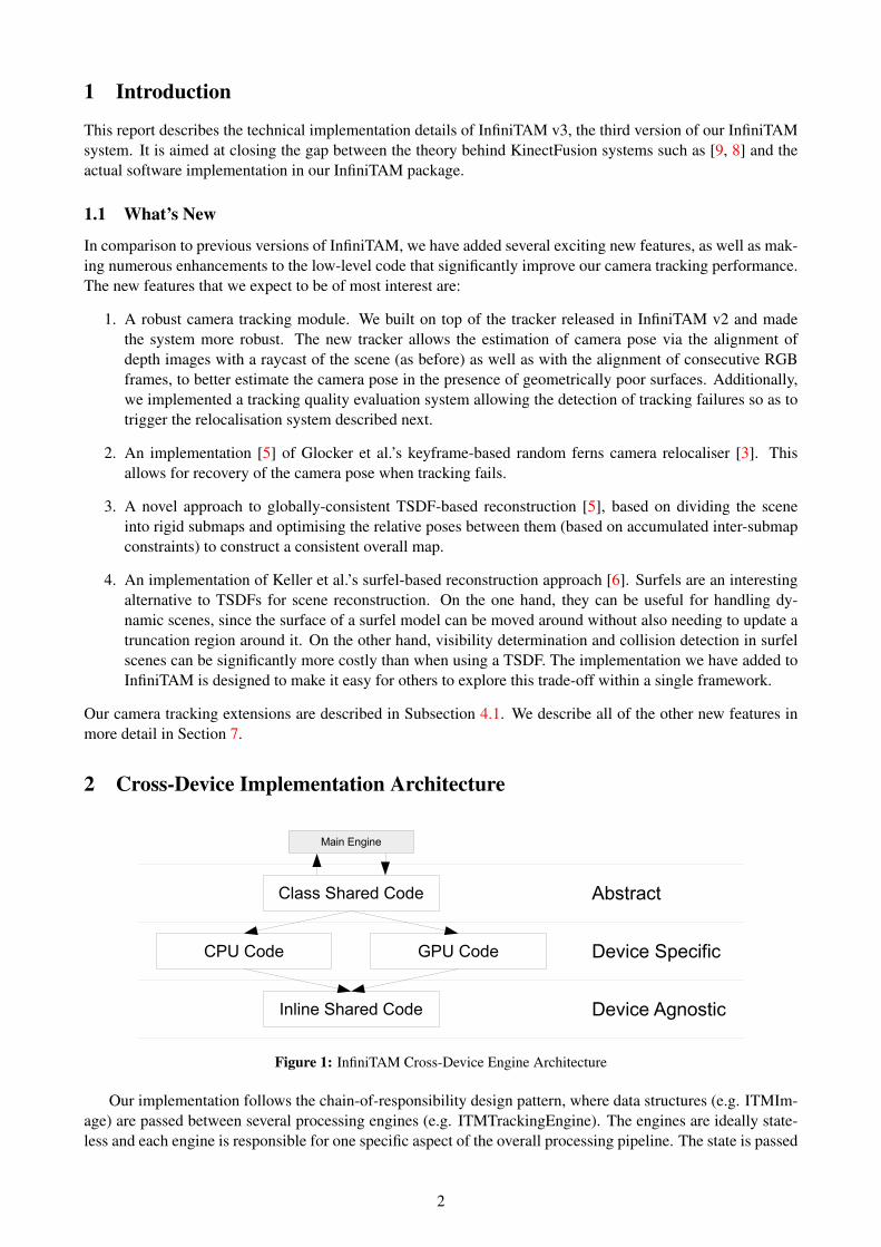
2 Cross-Device Implementation Architecture
Inline Shared Code
Abstract
CPU Code GPU Code Device Specific
Device Agnostic
Class Shared Code
Main Engine
Figure 1: InfiniTAM Cross-Device Engine Architecture
Our implementation follows the chain-of-responsibility design pattern, where data structures (e.g. ITMIm-age) are passed between several processing engines (e.g. ITMTrackingEngine). The engines are ideally state-less and each engine is responsible for one specific aspect of the overall processing pipeline. The state is passed
2
on in objects containing the processed information. Finally one parent class (ITMMainEngine) holds instancesof all objects and engines controls the flow of information.
Each engine is further split into 3 layers as shown in Figure 1. The topmost, so called Abstract Layer isaccessed by the library’s main engine and is in general just an abstract interface, although some common codemay be shared at this point. The abstract interface is implemented in the next, Device Specific Layer, whichmay be very different between e.g. a CPU and a GPU implementation. Further implementations using e.g.OpenMP or other hardware acceleration architectures are possible. At the third, Device Agnostic Layer, thereis some inline C-code that may be called from the higher layers.
For the example of a tracking engine, the Abstract Layer could contain code for generic optimization of anerror function, the Device Specific Layer could contain a loop or CUDA kernel call to evaluate the error functionfor all pixels in an image, and the Device Agnostic Layer contains a simple inline C-function to evaluate theerror in a single pixel.
Note that in InfiniTAM v3 the source code files have changed location. Whereas in InfiniTAM v2 there wasa single folder containing Device Agnostic and Device Specific files, we now provide separate folders for eachmodule (Tracking, Visualisation, etc.), each split into abstract, specific and agnostic.
3 Volumetric Representation with Hashes
The key component allowing InfiniTAM to scale KinectFusion to large scale 3D environments is the volumet-ric representation using a hash lookup, as also presented in [9]. This has remained mostly unchanged fromInfiniTAM v2.
The data structures and corresponding operations to implement this representation are as follows:
• Voxel Block Array: Holds the fused color and 3D depth information – details in Subsection 3.1.
• Hash Table and Hashing Function: Enable fast access to the voxel block array – details in Subsection 3.2.
• Hash Table Operations: Insertion, retrieval and deletion – details in Subsection 3.3.
3.1 The Voxel Block Array
Depth and (optionally) colour information is kept inside an ITMVoxel [s,f][ , rgb, conf] object:
s t r u c t I T M V o x e l t y p e v a r i a n t{
/∗ ∗ Value o f t h e t r u n c a t e d s i g n e d d i s t a n c e t r a n s f o r m a t i o n . ∗ /SDF DATA TYPE s d f ;/∗ ∗ Number o f f u s e d o b s e r v a t i o n s t h a t make up @p s d f . ∗ /u c h a r w depth ;/∗ ∗ RGB c o l o u r i n f o r m a t i o n s t o r e d f o r t h i s v o x e l . ∗ /Vec to r3u c l r ;/∗ ∗ Number o f o b s e r v a t i o n s t h a t made up @p c l r . ∗ /u c h a r w c o l o r ;
CPU AND GPU CODE ITMVoxel ( ){
s d f = SDF INITIAL VALUE ;w depth = 0 ;c l r = ( u c h a r ) 0 ;w c o l o r = 0 ;
}} ;
where (i) SDF DATA TYPE and SDF INITIAL VALUE depend on the type of depth representation, whichin the current implementation is either float, with initial value 1.0 (ITMVoxel f. . . ), or short, with initialvalue 32767 (ITMVoxel s. . . ), (ii) voxel types may or may not store colour information (ITMVoxel f rgband ITMVoxel s rgb) or confidence information (ITMVoxel f conf), and (iii) CPU AND GPU CODE definesmethods and functions that can be run both as host and as device code:
3
# i f d e f i n e d ( CUDACC ) && d e f i n e d ( CUDA ARCH )# d e f i n e CPU AND GPU CODE d e v i c e / / f o r CUDA d e v i c e code# e l s e# d e f i n e CPU AND GPU CODE# e n d i f
Voxels are grouped in blocks of predefined size (currently defined as 8× 8× 8). All the blocks are storedas a contiguous array, referred henceforth as the voxel block array or VBA. In the implementation this has adefined size of 218 elements.
3.2 The Hash Table and The Hashing Function
To quickly and efficiently find the position of a certain voxel block in the voxel block array, we use a hash table.This hash table is a contiguous array of ITMHashEntry objects of the following form:
s t r u c t ITMHashEntry{
/∗ ∗ P o s i t i o n o f t h e c o r n e r o f t h e 8 x8x8 volume , t h a t i d e n t i f i e s t h e e n t r y . ∗ /V e c t o r 3 s pos ;/∗ ∗ O f f s e t i n t h e e x c e s s l i s t . ∗ /i n t o f f s e t ;/∗ ∗ P o i n t e r t o t h e v o x e l b l o c k a r r a y .
− >= 0 i d e n t i f i e s an a c t u a l a l l o c a t e d e n t r y i n t h e v o x e l b l o c k a r r a y− −1 i d e n t i f i e s an e n t r y t h a t has been removed ( swapped o u t )− <−1 i d e n t i f i e s an u n a l l o c a t e d b l o c k
∗ /i n t p t r ;
} ;
The hash function hashIndex for locating entries of the hash table takes the corner coordinates blockPosof a 3D voxel block and computes an index as follows [9]:
t e m p l a t e<typename T> CPU AND GPU CODE i n l i n e i n t h a s h I n d e x ( c o n s t THREADPTR( T ) &b l o c kP o s )
{r e t u r n ( ( ( u i n t ) b l o ck P o s . x ∗ 73856093 u ) ˆ ( ( u i n t ) b l o c k P os . y ∗ 19349669 u ) ˆ ( ( u i n t )b l o c kP o s . z ∗ 83492791 u ) ) & ( u i n t )SDF HASH MASK ;
}
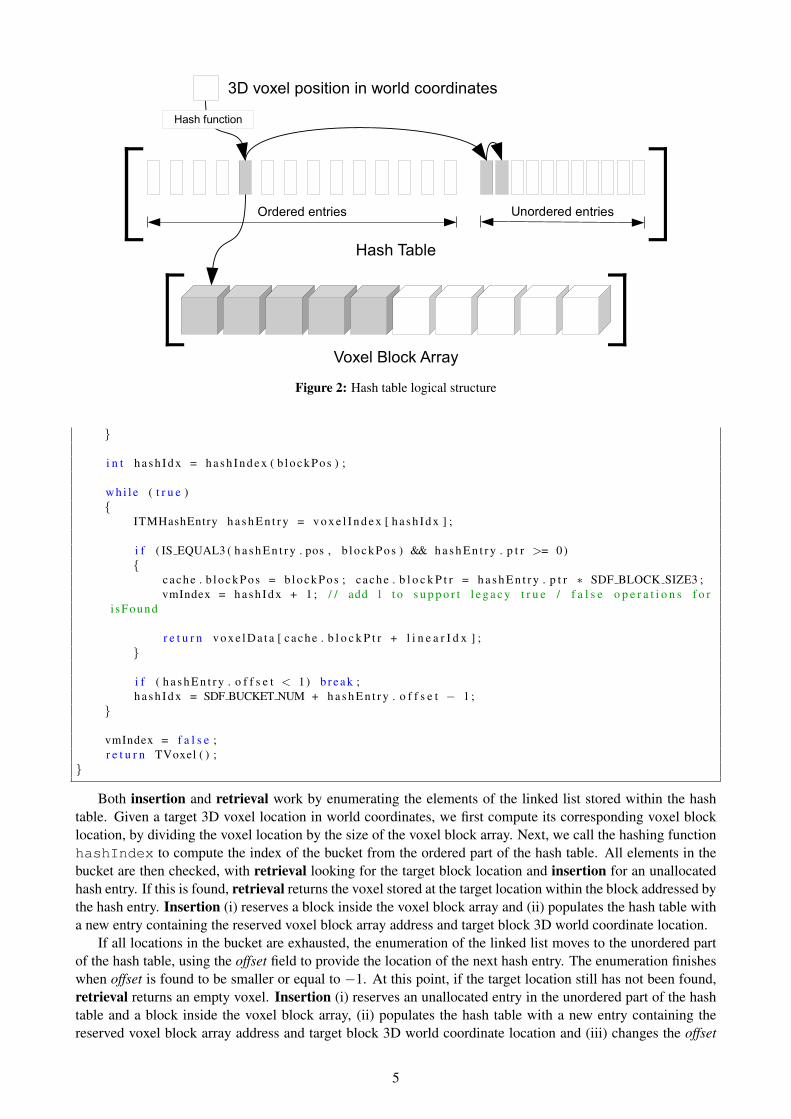
To deal with hash collisions, each hash index points to a bucket of size 1, which we consider the ordered partof the hash table. There is an additional unordered excess list that is used once an ordered bucket fills up. Ineither case, each ITMHashEntry in the hash table stores an offset in the voxel block array and can hence beused to localize the voxel data for each specific voxel block. This overall structure is illustrated in Figure 2.
3.3 Hash Table Operations
The three main operations used when working with a hash table are the insertion, retrieval and removal ofentries. In the current version of InfiniTAM we support the former two, with removal not currently required orimplemented. The code used by the retrieval operation is shown below:
t e m p l a t e<c l a s s TVoxel>CPU AND GPU CODE i n l i n e TVoxel r eadVoxe l ( c o n s t CONSTPTR( TVoxel ) ∗ voxe lDa ta , c o n s t
CONSTPTR( ITMLib : : ITMVoxelBlockHash : : IndexDa ta ) ∗ voxe l I ndex , c o n s t THREADPTR( V e c t o r 3 i )& p o i n t , THREADPTR( i n t ) &vmIndex , THREADPTR( ITMLib : : ITMVoxelBlockHash : : IndexCache ) &cache )
{V e c t o r 3 i b l o c k P o s ;i n t l i n e a r I d x = po in tToVoxe lB lockPos ( p o i n t , b l o c k P os ) ;
i f IS EQUAL3 ( blockPos , cache . b l oc k P o s ){
vmIndex = t r u e ;r e t u r n v o x e l D a t a [ cache . b l o c k P t r + l i n e a r I d x ] ;
4
3D voxel position in world coordinates
Ordered entries
Voxel Block Array
Hash Table
Hash function
Unordered entries
Figure 2: Hash table logical structure
}
i n t h a s h I d x = h a s h I n d e x ( b l o c k Po s ) ;
w h i l e ( t r u e ){
ITMHashEntry h a s h E n t r y = v o x e l I n d e x [ h a s h I d x ] ;
i f ( IS EQUAL3 ( h a s h E n t r y . pos , b l oc k P o s ) && h a s h E n t r y . p t r >= 0){
cache . b l o c k P os = b l o c k P o s ; cache . b l o c k P t r = h a s h E n t r y . p t r ∗ SDF BLOCK SIZE3 ;vmIndex = h a s h I d x + 1 ; / / add 1 t o s u p p o r t l e g a c y t r u e / f a l s e o p e r a t i o n s f o r
i sFound
r e t u r n v o x e l D a t a [ cache . b l o c k P t r + l i n e a r I d x ] ;}
i f ( h a s h E n t r y . o f f s e t < 1) b r e a k ;h a s h I d x = SDF BUCKET NUM + h a s h E n t r y . o f f s e t − 1 ;
}
vmIndex = f a l s e ;r e t u r n TVoxel ( ) ;
}
Both insertion and retrieval work by enumerating the elements of the linked list stored within the hashtable. Given a target 3D voxel location in world coordinates, we first compute its corresponding voxel blocklocation, by dividing the voxel location by the size of the voxel block array. Next, we call the hashing functionhashIndex to compute the index of the bucket from the ordered part of the hash table. All elements in thebucket are then checked, with retrieval looking for the target block location and insertion for an unallocatedhash entry. If this is found, retrieval returns the voxel stored at the target location within the block addressed bythe hash entry. Insertion (i) reserves a block inside the voxel block array and (ii) populates the hash table witha new entry containing the reserved voxel block array address and target block 3D world coordinate location.
If all locations in the bucket are exhausted, the enumeration of the linked list moves to the unordered partof the hash table, using the offset field to provide the location of the next hash entry. The enumeration finisheswhen offset is found to be smaller or equal to −1. At this point, if the target location still has not been found,retrieval returns an empty voxel. Insertion (i) reserves an unallocated entry in the unordered part of the hashtable and a block inside the voxel block array, (ii) populates the hash table with a new entry containing thereserved voxel block array address and target block 3D world coordinate location and (iii) changes the offset
5
field in the last found entry in the linked list to point to the newly populated one.The reserve operations used for the unordered part of the hash table and for the voxel block array use
prepopulated allocation lists and, in the GPU code, atomic operations.All hash table operations are done through these functions and there is no direct memory access encouraged
or indeed permitted by the current version of the code.
4 Method Stages
ITM Lib
ITM Low Level Engine ITM View Builder ITM Meshing Engine ITM Multi Meshing Engine
Swapping In
ITM SwappingEngine
Integration
ITM SceneReconstructionEngine
ITM Surfel Scene Reconstruction Engine
Raycast
ITM Visualisation Engine
ITM Multi Visualisation Engine
ITM Surfel Visualization Engine
Swapping Out
ITM SwappingEngine
Allocation
ITM SceneReconstructionEngine
ITM Surfel Scene Reconstruction Engine
Tracking
ITM Tracker
ITM Color Tracker
ITM Depth Tracker
ITM ExtendedTracker
UI Engine
InfiniTAM
ITM Main Engine
ITM Basic Engine
ITM Multi Engine
Relocaliser Fern Conservatory Pose Database
Fern Reloc Lib
Reloc Database
Image Source Engine OpenNI Engine RealSense Engine
Input Source
…
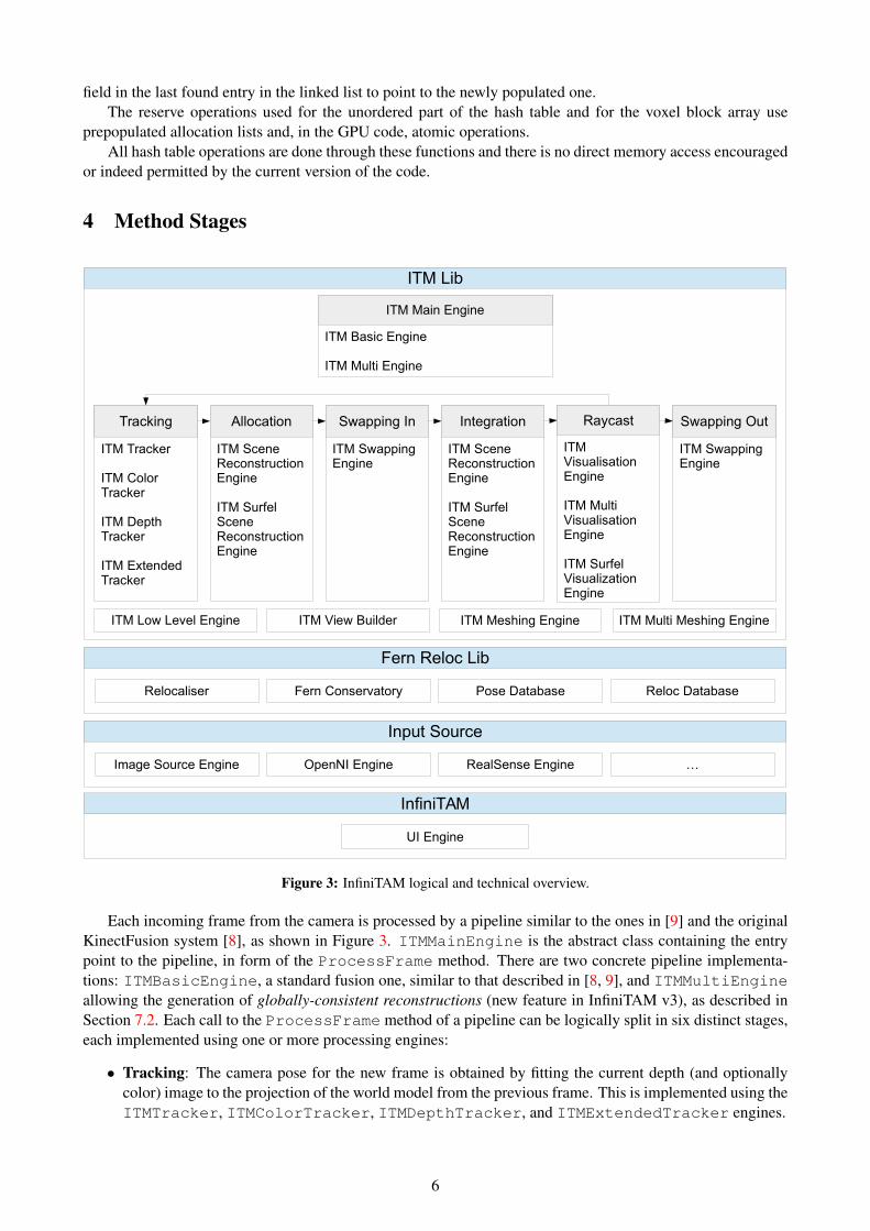
Figure 3: InfiniTAM logical and technical overview.
Each incoming frame from the camera is processed by a pipeline similar to the ones in [9] and the originalKinectFusion system [8], as shown in Figure 3. ITMMainEngine is the abstract class containing the entrypoint to the pipeline, in form of the ProcessFrame method. There are two concrete pipeline implementa-tions: ITMBasicEngine, a standard fusion one, similar to that described in [8, 9], and ITMMultiEngineallowing the generation of globally-consistent reconstructions (new feature in InfiniTAM v3), as described inSection 7.2. Each call to the ProcessFrame method of a pipeline can be logically split in six distinct stages,each implemented using one or more processing engines:
• Tracking: The camera pose for the new frame is obtained by fitting the current depth (and optionallycolor) image to the projection of the world model from the previous frame. This is implemented using theITMTracker, ITMColorTracker, ITMDepthTracker, and ITMExtendedTracker engines.
6
• Allocation: Based on the depth image, new voxel blocks are allocated as required and a list of all visiblevoxel blocks is built. This is implemented inside the ITMSceneReconstructionEngine (voxelmap) and ITMSurfelSceneReconstructionEngine classes (surfel map).
• Swapping In: If required, map data is swapped in from host memory to device memory. This is im-plemented using the ITMSwappingEngine. The current version only supports the BasicEngine withvoxels.
• Integration: The current depth and color frames are integrated within the map. Once again, this opera-tion is implemented inside the ITMSceneReconstructionEngine (map represented using voxels)and ITMSurfelSceneReconstructionEngine (surfel map) classes.
• Raycast: The world model is rendered from the current pose (i) for visualization purposes and (ii)to be used by the tracking stage at the next frame. This uses the ITMVisualisationEngine,ITMMultiVisualisationEngine, and ITMSurfelVisualisationEngine classes.
• Swapping Out: The parts of the map that are not visible are swapped out from device memory to hostmemory. This is implemented using the ITMSwappingEngine. The current version only supports theBasicEngine with voxels.
The main processing engines are contained within the ITMLib namespace, along with ITMLowLevelEngine,ITMViewBuilder, ITMMeshingEngine, and ITMMultiMeshingEngine. These are used, respec-tively, for low level processing (e.g. image copy, gradients and rescale), image preparation (converting depthimages from unsigned short to float values, normal computation, bilateral filtering), and mesh gener-ation via the Marching-Cubes algorithm [7].
The image acquisition routines, relying on a multitude of input sensors, can be found in the InputSourcenamespace, whilst the relocaliser implementation (another feature added in InfiniTAM v3 and described inSection. 7.1) is contained in the FernRelocLib namespace.
Finally, the main UI and the associated application are contained inside the InfiniTAM namespace.The following presents a discussion of the tracking, allocation, integration and raycast stages. We delay a
discussion of the swapping until Section 5.
4.1 Tracking
In the tracking stage we have to determine the pose of a new image given the 3D world model. We do thiseither based on the new depth image with an ITMDepthTracker, or based on the color image with anITMColorTracker. From version 3 of the InfiniTAM system, we also provide a revised and improvedtracking algorithm: ITMExtendedTracker. All extend the abstract ITMTracker class and have device-specific implementations running on the CPU and on CUDA.
4.1.1 ITMDepthTracker
In the ITMDepthTracker we follow the original alignment process as described in [8, 4]:
• Render a map V of surface points and a map N of surface normals from the viewpoint of an initial guess– details in Section 4.4
• Project all points p from the depth image onto points p in V and N and compute their distances fromthe planar approximation of the surface, i.e. d = (Rp+ t−V (p))T N (p)
• Find R and t minimizing of the sum of the squared distances by solving linear equation system
• Iterate the previous two steps until convergence
A resolution hierarchy of the depth image is used in our implementation to improve the convergence behaviour.
7

4.1.2 ITMColorTracker
Alternatively the color image can be used within an ITMColorTracker. In this case the alignment processis as follows:
• Create a list V of surface points and a corresponding list C of colours from the viewpoint of an initialguess – details in Section 4.4.
• Project all points from V into the current color image I and compute the difference in colours, i.e.d = ‖I(π(RV (i)+ t))−C (i)‖2.
• Find R and t minimizing of the sum of the squared differences using the Levenberg-Marquardt optimiza-tion algorithm.
Again a resolution hierarchy in the color image is used and the list of surface points is subsampled by a factorof 4.
4.1.3 ITMExtendedTracker
The ITMExtendedTracker class allows the alignment of the current RGB-D image captured by the sensorin a manner analogous to that described in Section 4.1.1.
More specifically, in its default configuration, an instance of ITMExtendedTracker can seamlesslyreplace an ITMDepthTracker whilst providing typically better tracking accuracy. The main differenceswith a simple ICP-based tracker (such as the one previously implemented – and described in [8, 4]) are asfollows:
• A robust Huber-norm is deployed instead of the quite standard L2 norm when computing the error termassociated to each pixel of the input depth image.
• The error term for each pixel of the depth image, in addition to being subject to the robust norm justdescribed, is weighted according to its depth measurement provided by the sensor, so as to accountfor the noisier nature of distance measurements associated to points far away from the camera (weightdecreases with the increase in distance reading).
• Points p whose projection p in V have a distance from the planar approximation of the surface d =(Rp+ t−V (p))T N (p) greater than a configurable threshold, are not considered in the error functionbeing minimised, as they are likely outliers.
• Finally, as described in Section 2.2 of [5], the results of the ICP optimisation phase (percentage of inlierpixels, determinant of the Hessian and residual sum) are evaluated by an SVM classifier to separatebetween tracking success and failure, as well as to establish whether a successful result has good or badaccuracy. In case of tracking failure, the relocaliser described in Section 7.1 is activated to attempt theestimation of the current camera pose and recover the localisation and mapping loop.
The capabilities of the ITMExtendedTracker class are not limited to a better ICP-based camera track-ing step. The user can, optionally, achieve a combined geometric-photometric alignment as well.
As in [11], we augment the extended tracker’s geometric error term described above with a per-pixel pho-tometric error term. In more detail, we try to minimise the difference in intensity between each pixel in thecurrent RGB image and the corresponding pixel in the previous frame captured by the sensor (note that, dif-ferently from the ITMColorTracker described in the previous section, we do not need to have access to acoloured reconstruction, since we do not make use of voxel colours in the matching phase). Frame-to-framepixel intensity differences are estimated as follows:
1. The intensity and depth value associated to a pixel in the current RGB-D pair are sampled from theimages (each intensity value I is computed as a weighted average of the RGB colour channels: I =0.299R+0.587G+0.114B).
2. 3D coordinates of the pixel in the current camera’s reference frame are computed by backprojecting itsdepth value according to the camera intrinsic parameters.
8
3. Given a candidate sensor pose (the initial guess also used to compute the geometric error term), the 3Dpixel coordinates are brought into a scene coordinate frame.
4. Use the previous frame’s estimated pose to bring the pixel coordinates back to the previous camera’sreference frame.
5. Project those coordinates onto the previous RGB image and compute the intensity of the sampled pointby bilinearly interpolating values associated to its neighbouring pixels.
The sum of per-pixel intensity differences over the whole image – as before, subject to depth-based weight-ing and robust loss function (we use Tukey’s in this case) – is added to the geometric error term describedabove using an appropriate scaling factor, to account for the different ranges of the values (0.3 in the currentimplementation). Gradient and Hessian values are combined as well. A Levenberg-Marquardt optimizationalgorithm is then deployed to minimise the error and estimate the final pose.
As with the other trackers, a resolution hierarchy is computed, and the camera alignment is performedstarting from the coarsest resolution to the finest one, to improve the convergence behaviour.
4.1.4 Configuration
A string in ITMLibSettings allows to select which tracker to use, as well as specifying tracker-specificconfiguration values. By default an instance of ITMExtendedTracker (with the colour-tracking energyterm disabled – to allow for the employment of depth-only sensors such as Occipital’s Structure1) is created.Other configuration strings can be found (as comments) in ITMLib/Utils/ITMLibSettings.cpp.
All tracker implementations use the device (in the CUDA-specific subclass, relying on the CPU otherwise)only for the computation of function, gradient and Hessian values. Everything else, such as the optimisation, isdone in the main, abstract class.
4.2 Allocation
The allocation stage is split into three separate parts. Our aim here was minimise the use of blocking operations(e.g. atomics) and completely avoid the use of critical sections.
Firstly, for each 2.5D pixel from the depth image, we backproject a line connecting d−µ to d+µ , where dis the depth in image coordinates and µ is a fixed, tunable parameter. This leads to a line in world coordinates,which intersects a number of voxel blocks. We search the hash table for each of these blocks and look fora free hash entry for each unallocated one. These memorised for the next stage of the allocation using twoarrays, each with the same number of elements as the hash table, containing information about the allocationand visibility of the new hash entries. Note that, if two or more blocks for the same depth image are mappedto the same hash entry (i.e. if we have intra-frame hash collisions), only one will be allocated. This artefact isfixed automatically at the next frame, as the intra-frame camera motion is relatively small.
Secondly, we allocate voxel blocks for each non zero entry in the allocation and visibility arrays builtpreviously. This is done using atomic subtraction on a stack of free voxel block indices i.e. we decrease thenumber of available blocks by one and add the previous head of the stack to the hash entry.
Thirdly, we build a list of live hash entries, i.e. containing the ones that project inside the visible frustum.This is later going to be used by the integration and swapping in/out stages.
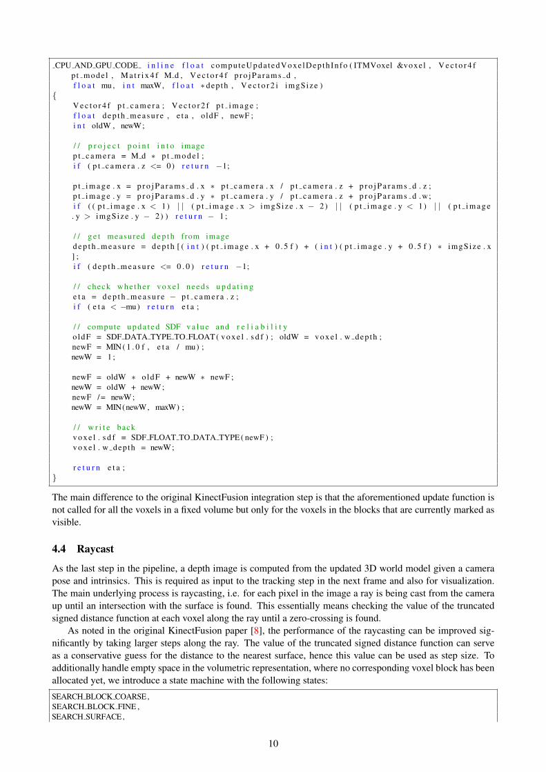
4.3 Integration
In the integration stage, the information from the most recent images is incorporated into the 3D world model.This is done essentially the same way as in the original KinectFusion algorithm [8, 4]. For each voxel inany of the visible voxel blocks from above the function computeUpdatedVoxelDepthInfo is called.If a voxel is behind the surface observed in the new depth image, the image does not contain any new in-formation about it, and the function returns. If the voxel is close to or in front of the observed surface, acorresponding observation is added to the accumulated sum. This is illustrated in the listing of the functioncomputeUpdatedVoxelDepthInfo below.
1https://structure.io/
9
CPU AND GPU CODE i n l i n e f l o a t computeUpda tedVoxe lDep th In fo ( ITMVoxel &voxel , V e c t o r 4 fp t mode l , M a t r i x 4 f M d , V e c t o r 4 f p r o j P a r a m s d ,f l o a t mu , i n t maxW, f l o a t ∗ depth , V e c t o r 2 i imgSize )
{V e c t o r 4 f p t c a m e r a ; V e c t o r 2 f p t i m a g e ;f l o a t d e p th m ea s u re , e t a , oldF , newF ;i n t oldW , newW;
/ / p r o j e c t p o i n t i n t o imagep t c a m e r a = M d ∗ p t m o d e l ;i f ( p t c a m e r a . z <= 0) r e t u r n −1;
p t i m a g e . x = p r o j P a r a m s d . x ∗ p t c a m e r a . x / p t c a m e r a . z + p r o j P a r a m s d . z ;p t i m a g e . y = p r o j P a r a m s d . y ∗ p t c a m e r a . y / p t c a m e r a . z + p r o j P a r a m s d .w;i f ( ( p t i m a g e . x < 1) | | ( p t i m a g e . x > imgSize . x − 2) | | ( p t i m a g e . y < 1) | | ( p t i m a g e. y > imgSize . y − 2) ) r e t u r n − 1 ;
/ / g e t measured d e p t h from imaged e p t h m e a s u r e = d e p t h [ ( i n t ) ( p t i m a g e . x + 0 . 5 f ) + ( i n t ) ( p t i m a g e . y + 0 . 5 f ) ∗ imgSize . x] ;i f ( d e p t h m e a s u r e <= 0 . 0 ) r e t u r n −1;
/ / check whe the r v o x e l needs u p d a t i n ge t a = d e p t h m e a s u r e − p t c a m e r a . z ;i f ( e t a < −mu) r e t u r n e t a ;
/ / compute u p d a t e d SDF v a l u e and r e l i a b i l i t yo ldF = SDF DATA TYPE TO FLOAT ( v o x e l . s d f ) ; oldW = v o x e l . w depth ;newF = MIN ( 1 . 0 f , e t a / mu) ;newW = 1 ;
newF = oldW ∗ oldF + newW ∗ newF ;newW = oldW + newW;newF /= newW;newW = MIN(newW, maxW) ;
/ / w r i t e backv o x e l . s d f = SDF FLOAT TO DATA TYPE ( newF ) ;v o x e l . w depth = newW;
r e t u r n e t a ;}
The main difference to the original KinectFusion integration step is that the aforementioned update function isnot called for all the voxels in a fixed volume but only for the voxels in the blocks that are currently marked asvisible.
4.4 Raycast
As the last step in the pipeline, a depth image is computed from the updated 3D world model given a camerapose and intrinsics. This is required as input to the tracking step in the next frame and also for visualization.The main underlying process is raycasting, i.e. for each pixel in the image a ray is being cast from the cameraup until an intersection with the surface is found. This essentially means checking the value of the truncatedsigned distance function at each voxel along the ray until a zero-crossing is found.
As noted in the original KinectFusion paper [8], the performance of the raycasting can be improved sig-nificantly by taking larger steps along the ray. The value of the truncated signed distance function can serveas a conservative guess for the distance to the nearest surface, hence this value can be used as step size. Toadditionally handle empty space in the volumetric representation, where no corresponding voxel block has beenallocated yet, we introduce a state machine with the following states:
SEARCH BLOCK COARSE,SEARCH BLOCK FINE ,SEARCH SURFACE,
10
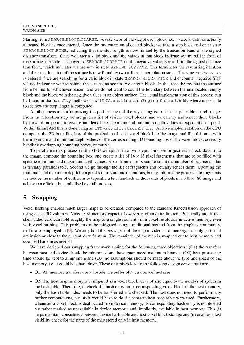
BEHIND SURFACE ,WRONG SIDE
Starting from SEARCH BLOCK COARSE, we take steps of the size of each block, i.e. 8 voxels, until an actuallyallocated block is encountered. Once the ray enters an allocated block, we take a step back and enter stateSEARCH BLOCK FINE, indicating that the step length is now limited by the truncation band of the signeddistance transform. Once we enter a valid block and the values in that block indicate we are still in front ofthe surface, the state is changed to SEARCH SURFACE until a negative value is read from the signed distancetransform, which indicates we are now in state BEHIND SURFACE. This terminates the raycasting iterationand the exact location of the surface is now found by two trilinear interpolation steps. The state WRONG SIDEis entered if we are searching for a valid block in state SEARCH BLOCK FINE and encounter negative SDFvalues, indicating we are behind the surface, as soon as we enter a block. In this case the ray hits the surfacefrom behind for whichever reason, and we do not want to count the boundary between the unallocated, emptyblock and the block with the negative values as an object surface. The actual implementation of this process canbe found in the castRay method of the ITMVisualisationEngine Shared.h file where is possibleto see how the step length is computed.
Another measure for improving the performance of the raycasting is to select a plausible search range.From the allocation step we are given a list of visible voxel blocks, and we can try and render these blocksby forward projection to give us an idea of the maximum and minimum depth values to expect at each pixel.Within InfiniTAM this is done using an ITMVisualisationEngine. A naive implementation on the CPUcomputes the 2D bounding box of the projection of each voxel block into the image and fills this area withthe maximum and minimum depth values of the corresponding 3D bounding box of the voxel block, correctlyhandling overlapping bounding boxes, of course.
To parallelise this process on the GPU we split it into two steps. First we project each block down intothe image, compute the bounding box, and create a list of 16× 16 pixel fragments, that are to be filled withspecific minimum and maximum depth values. Apart from a prefix sum to count the number of fragments, thisis trivially parallelisable. Second we go through the list of fragments and actually render them. Updating theminimum and maximum depth for a pixel requires atomic operations, but by splitting the process into fragmentswe reduce the number of collisions to typically a few hundreds or thousands of pixels in a 640×480 image andachieve an efficiently parallelised overall process.
5 Swapping
Voxel hashing enables much larger maps to be created, compared to the standard KinectFusion approach ofusing dense 3D volumes. Video card memory capacity however is often quite limited. Practically an off-the-shelf video card can hold roughly the map of a single room at 4mm voxel resolution in active memory, evenwith voxel hashing. This problem can be mitigated using a traditional method from the graphics community,that is also employed in [9]. We only hold the active part of the map in video card memory, i.e. only parts thatare inside or close to the current view frustum. The remainder of the map is swapped out to host memory andswapped back in as needed.
We have designed our swapping framework aiming for the following three objectives: (O1) the transfersbetween host and device should be minimized and have guaranteed maximum bounds, (O2) host processingtime should be kept to a minimum and (O3) no assumptions should be made about the type and speed of thehost memory, i.e. it could be a hard drive. These objectives lead to the following design considerations:
• O1: All memory transfers use a host/device buffer of fixed user-defined size.
• O2: The host map memory is configured as a voxel block array of size equal to the number of spaces inthe hash table. Therefore, to check if a hash entry has a corresponding voxel block in the host memory,only the hash table index needs to be transferred and checked. The host does not need to perform anyfurther computations, e.g. as it would have to do if a separate host hash table were used. Furthermore,whenever a voxel block is deallocated from device memory, its corresponding hash entry is not deletedbut rather marked as unavailable in device memory, and, implicitly, available in host memory. This (i)helps maintain consistency between device hash table and host voxel block storage and (ii) enables a fastvisibility check for the parts of the map stored only in host memory.
11

• O3: Global memory speed is a function of the type of storage device used, e.g. faster for RAM and slowerfor flash or hard drive storage. This means that, for certain configurations, host memory operations canbe considerably slower than the device reconstruction. To account for this behaviour and to enable stabletracking, the device is constantly integrating new live depth data even for parts of the scene that are knownto have host data that is not yet in device memory. This might mean that, by the time all visible partsof the scene have been swapped into the device memory, some voxel blocks might hold large amountsof new data integrated by the device. We could replace the newly fused data with the old one from thehost stored map, but this would mean disregarding perfectly fine map data. Instead, after the swappingoperation, we run a secondary integration that fuses the host voxel block data with the newly fused devicemap.
Allocation Populate cacheFromHost.
Integration Populate cacheToHost.
Swap In
→ Build list of needed voxel blocks.→ Copy list to host memory.→ Populate transfer buffer according to list.→ Copy voxel transfer buffer to device memory.→ Integrate transferred block into device memory.
Raycast
Swap Out
→ Build list of transferring voxel blocks.→ Populate transfer buffer according to list.→ Delete transferring blocks from voxel block array.→ Copy voxel transfer buffer to host memory.→ Update global memory with transferred blocks.
Tracking
Figure 4: Swapping pipeline
The design considerations have led us to the swapping in/out pipeline shown in Figure 4. We use theallocation stage to establish which parts of the map need to be swapped in, and the integration stage to markwhich parts need to swapped out. A voxel needs to be swapped (i) from host once it projects within a small(tunable) distance from the boundaries of live visible frame and (ii) to disk after data has been integrated fromthe depth camera.
The swapping in stage is exemplified for a single block in Figure 5. The indices of the hash entries thatneed to be swapped in are copied into the device transfer buffer, up to its capacity. Next, this is transferred tothe host transfer buffer. There the indices are used as addresses inside the host voxel block array and the targetblocks are copied to the host transfer buffer. Finally, the host transfer buffer is copied to the device where asingle kernel integrates directly from the transfer buffer into the device voxel block memory.
An example for the swapping out stage is shown in Figure 6 for a single block. Both indices and voxelblocks that need to be swapped out are copied to the device transfer buffer. This is then copied to the hosttransfer buffer memory and again to host voxel memory.
All swapping related variables and memory is kept inside the ITMGlobalCache object and all swappingrelated operations are done by the ITMSwappingEngine.
6 UI, Usage and Examples
The UI for our implementation is shown in Figure 7. We show a live raycasted rendering of the reconstruction,live depth image and live colour image, along with the processing time per frame and the keyboard shortcutsavailable for the UI. The user can choose to process one frame at a time or process the whole input video
12

4
1
7
3
5
2
6
Device Voxel Memory
Hash Table
Transfer Buffer
Host Voxel Memory
Figure 5: Swapping in: First, the hash table entry at address 1 is copied into the device transfer buffer at address 2. Thisis then copied at address 3 in the host transfer buffer and used as an address inside the host voxel block array, indicatingthe block at address 4. This block is finally copied back to location 7 inside the device voxel block array, passing throughthe host transfer buffer (location 5) and the device transfer buffer (location 6).
7
1
3
5
5
2
4
Device Voxel Memory
Hash Table
Transfer Buffer
Host Voxel Memory
Figure 6: Swapping Out. The hash table entry at location 1 and the voxel block at location 3 are copied into the devicetransfer buffer at locations 2 and 4, respectively. The entire used transfer buffer is then copied to the host, at locations 5,and the hash entry index is used to copy the voxel block into location 7 inside the host voxel block array.
13

Reconstruction Live depth image Live colour image
Keyboard shortcuts Processing time per frame
Figure 7: InfiniTAM UI Example
stream. Other functionalities such as resetting the InfiniTAM system, exporting a 3D model from the recon-struction, arbitrary view raycast and different rendering styles are also available. The UI window and behaviouris implemented in UIEngine and requires OpenGL and GLUT.
Running InfiniTAM requires a calibrated data source of depth (and optionally image). The calibration isspecified through an external file, an example of which is shown below.
640 480504 .261 503 .905352 .457 272 .202
640 480573 .71 574 .394346 .471 249 .031
0 .999749 0 .00518867 0 .0217975 0 .0243073−0.0051649 0 .999986 −0.0011465 −0.000166518−0.0218031 0 .00103363 0 .999762 0 .0151706
1135 .09 0 .0819141
This includes (i) for the each camera (RGB or depth) the image size, focal length and principal point (in pixels),as outputted by the Matlab Calibration Toolbox [1] (ii) the extrinsic matrix mapping depth into RGB coordinatesobtained and (iii) the calibration of the depth.
We also provide several data sources in the InputSource namespace, examples of those are OpenNI andimage files. We tested OpenNI with PrimeSense-based long range depth camera, the Kinect Sensor, RealSensecameras and the Structure Sensor; whereas images need to be in the PPM/PGM format. When only depth isprovided (such as e.g. by the Structure Sensor) InfiniTAM will only function with the ICP depth-based tracker.
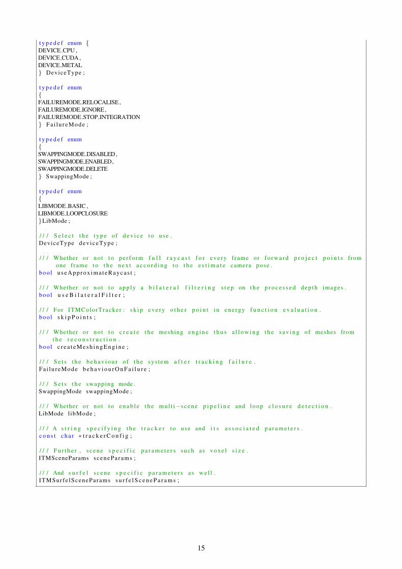
All library settings are defined inside the ITMLibSettings class, and are:
c l a s s I T M L i b S e t t i n g s{p u b l i c :/ / / The d e v i c e used t o run t h e D e v i c e A g n o s t i c code
14
t y p e d e f enum {DEVICE CPU ,DEVICE CUDA ,DEVICE METAL} DeviceType ;
t y p e d e f enum{FAILUREMODE RELOCALISE ,FAILUREMODE IGNORE,FAILUREMODE STOP INTEGRATION} Fa i lu reMode ;
t y p e d e f enum{SWAPPINGMODE DISABLED,SWAPPINGMODE ENABLED,SWAPPINGMODE DELETE} SwappingMode ;
t y p e d e f enum{LIBMODE BASIC ,LIBMODE LOOPCLOSURE}LibMode ;
/ / / S e l e c t t h e t y p e o f d e v i c e t o use .DeviceType dev iceType ;
/ / / Whether o r n o t t o pe r fo rm f u l l r a y c a s t f o r e v e r y f rame or f o r w a r d p r o j e c t p o i n t s fromone f rame t o t h e n e x t a c c o r d i n g t o t h e e s t i m a t e camera pose .
boo l u s e A p p r o x i m a t e R a y c a s t ;
/ / / Whether o r n o t t o a p p l y a b i l a t e r a l f i l t e r i n g s t e p on t h e p r o c e s s e d d e p t h images .boo l u s e B i l a t e r a l F i l t e r ;
/ / / For ITMColorTracker : s k i p e v e r y o t h e r p o i n t i n e ne rg y f u n c t i o n e v a l u a t i o n .boo l s k i p P o i n t s ;
/ / / Whether o r n o t t o c r e a t e t h e meshing e n g i n e t h u s a l l o w i n g t h e s a v i n g of meshes fromt h e r e c o n s t r u c t i o n .
boo l c r e a t e M e s h i n g E n g i n e ;
/ / / S e t s t h e b e h a v i o u r o f t h e sys tem a f t e r t r a c k i n g f a i l u r e .Fa i lu reMode b e h a v i o u r O n F a i l u r e ;
/ / / S e t s t h e swapping mode .SwappingMode swappingMode ;
/ / / Whether o r n o t t o e n a b l e t h e m u l t i−s c e n e p i p e l i n e and loop c l o s u r e d e t e c t i o n .LibMode l ibMode ;
/ / / A s t r i n g s p e c i f y i n g t h e t r a c k e r t o use and i t s a s s o c i a t e d p a r a m e t e r s .c o n s t c h a r ∗ t r a c k e r C o n f i g ;
/ / / F u r t h e r , s c e n e s p e c i f i c p a r a m e t e r s such as v o x e l s i z e .ITMSceneParams sceneParams ;
/ / / And s u r f e l s c e n e s p e c i f i c p a r a m e t e r s a s w e l l .ITMSurfe lSceneParams s u r f e l S c e n e P a r a m s ;
15
7 New Features in InfiniTAM v3
7.1 Random Ferns Relocaliser
One of the key new features that has been added to InfiniTAM since the previous version is an implementation[5] of Glocker et al.’s keyframe-based random ferns camera relocaliser [3]. This can be used both to relocalisethe camera when tracking fails, and to detect loop closures when aiming to construct a globally-consistent scene(see Subsection 7.2). Relocalisation using random ferns is comparatively straightforward. We provide a briefsummary here that broadly follows the presentation in [3]. Further details can be found in the original paper.
At the core of the approach is a method for encoding an RGB-D image I as a set of m binary code blocks,each of length n. Each of the m code blocks is obtained by applying a random fern to I, where a fern is a set ofn binary feature tests on the image, each yielding either 0 or 1. Letting bI
Fk∈ Bn denote the n-bit binary code
resulting from applying fern Fk to I, and bIC ∈ Bmn denote the result of concatenating all m such binary codes
for I, it is possible to define a dissimilarity measure between two different images I and J as the block-wiseHamming distance between bI
C and bJC. In other words,
BlockHD(bIC,b
JC) =
1m
m
∑k=1
(bIFk≡ bJ
Fk), (1)
where (bIFk≡ bJ
Fk) is 0 if the two code blocks are identical, and 1 otherwise.
Given this approach to image encoding, the idea behind the relocaliser is conceptually to learn a lookuptable from encodings of keyframe images to their known camera poses (e.g. as obtained during a successfulinitial tracking phase). Relocalisation can then be attempted by finding the nearest neighbour(s) of the encodingof the current camera input image in this table, and trying to use their recorded pose(s) to restart tracking. Inpractice, a slightly more sophisticated scheme is used. Instead of maintaining a lookup table from encodingsto known camera poses, the approach maintains (i) a global lookup table P that maps keyframe IDs to knowncamera poses, and (ii) a set of m code tables (one per fern) that map each of the 2n possible binary codesresulting from applying a fern to an image to the IDs of the keyframes that achieve that binary code.
This layout makes it easy to find, for each incoming camera input image I, the most similar keyframe(s)currently stored in the relocaliser: specifically, it suffices to compute the m code blocks for I and use the codetables to look up all the keyframes with which I shares at least one code block in common. The similarity ofeach such keyframe to I can then be trivially computed, allowing the keyframes to be ranked in descendingorder of similarity. During the training phase, this is used to decide whether to add a new keyframe to therelocaliser. If the most similar keyframe currently stored is sufficiently dissimilar to the current camera inputimage I, a new entry for I is added to the global lookup table and the code tables are updated based on I’s codeblocks. During the relocalisation phase, the nearest keyframe(s) to the camera input image are simply lookedup, and their poses are used to try to restart tracking.
The implementation of this approach in InfiniTAM can be found in the FernRelocLib library. Theferns to be applied to an image are stored in a FernConservatory. The computeCode function inFernConservatory computes the actual binary codes. The global lookup table is implemented in thePoseDatabase class, and the code tables are implemented in the RelocDatabase class. Finally, ev-erything is tied together by the top-level Relocaliser class, which provides the public interface to therelocaliser. For readers who want to better understand how the code works, a good place to start is theProcessFrame function in Relocaliser.
Limitations. The random ferns approach to relocalisation has a number of advantages: it is easy to imple-ment, fast to run, and performs well when relocalising from poses that correspond to stored keyframes. How-ever, because it is a keyframe-based approach, it tends to relocalise poorly from novel poses. If desired, betterrelocalisation from novel poses can be obtained using correspondence-based methods, e.g. the scene coordinateregression forests of Shotton et al. [10]. The original implementation of this approach required extensive pre-training on the scene of interest, making it impractical for online relocalisation, but recent work by Cavallari etal. [2] has removed this limitation.
16
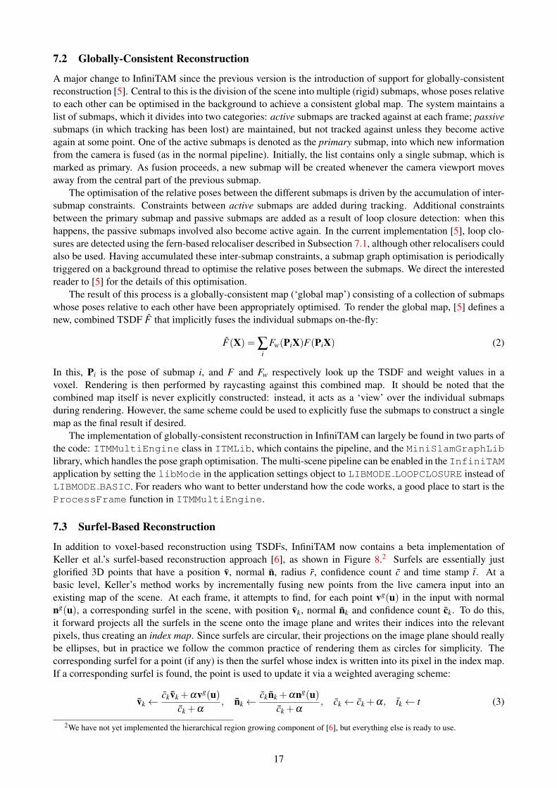
7.2 Globally-Consistent Reconstruction
A major change to InfiniTAM since the previous version is the introduction of support for globally-consistentreconstruction [5]. Central to this is the division of the scene into multiple (rigid) submaps, whose poses relativeto each other can be optimised in the background to achieve a consistent global map. The system maintains alist of submaps, which it divides into two categories: active submaps are tracked against at each frame; passivesubmaps (in which tracking has been lost) are maintained, but not tracked against unless they become activeagain at some point. One of the active submaps is denoted as the primary submap, into which new informationfrom the camera is fused (as in the normal pipeline). Initially, the list contains only a single submap, which ismarked as primary. As fusion proceeds, a new submap will be created whenever the camera viewport movesaway from the central part of the previous submap.
The optimisation of the relative poses between the different submaps is driven by the accumulation of inter-submap constraints. Constraints between active submaps are added during tracking. Additional constraintsbetween the primary submap and passive submaps are added as a result of loop closure detection: when thishappens, the passive submaps involved also become active again. In the current implementation [5], loop clo-sures are detected using the fern-based relocaliser described in Subsection 7.1, although other relocalisers couldalso be used. Having accumulated these inter-submap constraints, a submap graph optimisation is periodicallytriggered on a background thread to optimise the relative poses between the submaps. We direct the interestedreader to [5] for the details of this optimisation.
The result of this process is a globally-consistent map (‘global map’) consisting of a collection of submapswhose poses relative to each other have been appropriately optimised. To render the global map, [5] defines anew, combined TSDF F that implicitly fuses the individual submaps on-the-fly:
F(X) = ∑i
Fw(PiX)F(PiX) (2)
In this, Pi is the pose of submap i, and F and Fw respectively look up the TSDF and weight values in avoxel. Rendering is then performed by raycasting against this combined map. It should be noted that thecombined map itself is never explicitly constructed: instead, it acts as a ‘view’ over the individual submapsduring rendering. However, the same scheme could be used to explicitly fuse the submaps to construct a singlemap as the final result if desired.
The implementation of globally-consistent reconstruction in InfiniTAM can largely be found in two parts ofthe code: ITMMultiEngine class in ITMLib, which contains the pipeline, and the MiniSlamGraphLiblibrary, which handles the pose graph optimisation. The multi-scene pipeline can be enabled in the InfiniTAMapplication by setting the libMode in the application settings object to LIBMODE LOOPCLOSURE instead ofLIBMODE BASIC. For readers who want to better understand how the code works, a good place to start is theProcessFrame function in ITMMultiEngine.
7.3 Surfel-Based Reconstruction
In addition to voxel-based reconstruction using TSDFs, InfiniTAM now contains a beta implementation ofKeller et al.’s surfel-based reconstruction approach [6], as shown in Figure 8.2 Surfels are essentially justglorified 3D points that have a position v, normal n, radius r, confidence count c and time stamp t. At abasic level, Keller’s method works by incrementally fusing new points from the live camera input into anexisting map of the scene. At each frame, it attempts to find, for each point vg(u) in the input with normalng(u), a corresponding surfel in the scene, with position vk, normal nk and confidence count ck. To do this,it forward projects all the surfels in the scene onto the image plane and writes their indices into the relevantpixels, thus creating an index map. Since surfels are circular, their projections on the image plane should reallybe ellipses, but in practice we follow the common practice of rendering them as circles for simplicity. Thecorresponding surfel for a point (if any) is then the surfel whose index is written into its pixel in the index map.If a corresponding surfel is found, the point is used to update it via a weighted averaging scheme:
vk←ckvk +αvg(u)
ck +α, nk←
cknk +αng(u)ck +α
, ck← ck +α, tk← t (3)
2We have not yet implemented the hierarchical region growing component of [6], but everything else is ready to use.
17
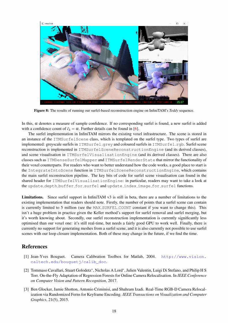
Figure 8: The results of running our surfel-based reconstruction engine on InfiniTAM’s Teddy sequence.
In this, α denotes a measure of sample confidence. If no corresponding surfel is found, a new surfel is addedwith a confidence count of ck = α . Further details can be found in [6].
The surfel implementation in InfiniTAM mirrors the existing voxel infrastructure. The scene is stored inan instance of the ITMSurfelScene class, which is templated on the surfel type. Two types of surfel areimplemented: greyscale surfels in ITMSurfel grey and coloured surfels in ITMSurfel rgb. Surfel scenereconstruction is implemented in ITMSurfelSceneReconstructionEngine (and its derived classes),and scene visualisation in ITMSurfelVisualisationEngine (and its derived classes). There are alsoclasses such as ITMDenseSurfelMapper and ITMSurfelRenderState that mirror the functionality oftheir voxel counterparts. For readers who want to better understand how the code works, a good place to start isthe IntegrateIntoScene function in ITMSurfelSceneReconstructionEngine, which containsthe main surfel reconstruction pipeline. The key bits of code for surfel scene visualisation can found in theshared header for ITMSurfelVisualisationEngine: in particular, readers may want to take a look atthe update depth buffer for surfel and update index image for surfel functions.
Limitations. Since surfel support in InfiniTAM v3 is still in beta, there are a number of limitations to theexisting implementation that readers should note. Firstly, the number of points that a surfel scene can containis currently limited to 5 million (see the MAX SURFEL COUNT constant if you want to change this). Thisisn’t a huge problem in practice given the Keller method’s support for surfel removal and surfel merging, butit’s worth knowing about. Secondly, our surfel reconstruction implementation is currently significantly lessoptimised than our voxel one: it’s still real-time, but needs a fairly good GPU to work well. Finally, there iscurrently no support for generating meshes from a surfel scene, and it is also currently not possible to use surfelscenes with our loop closure implementation. Both of these may change in the future, if we find the time.
References
[1] Jean-Yves Bouguet. Camera Calibration Toolbox for Matlab, 2004. http://www.vision.caltech.edu/bouguetj/calib_doc.
[2] Tommaso Cavallari, Stuart Golodetz∗, Nicholas A Lord∗, Julien Valentin, Luigi Di Stefano, and Philip H STorr. On-the-Fly Adaptation of Regression Forests for Online Camera Relocalisation. In IEEE Conferenceon Computer Vision and Pattern Recognition, 2017.
[3] Ben Glocker, Jamie Shotton, Antonio Criminisi, and Shahram Izadi. Real-Time RGB-D Camera Relocal-ization via Randomized Ferns for Keyframe Encoding. IEEE Transactions on Visualization and ComputerGraphics, 21(5), 2015.
18
[4] Shahram Izadi, David Kim, Otmar Hilliges, David Molyneaux, Richard Newcombe, Pushmeet Kohli,Jamie Shotton, Steve Hodges, Dustin Freeman, Andrew Davison, and Andrew Fitzgibbon. KinectFusion:Real-time 3D Reconstruction and Interaction Using a Moving Depth Camera. In Proceedings of the 24thAnnual ACM Symposium on User Interface Software and Technology, pages 559–568, 2011.
[5] Olaf Kahler, Victor A Prisacariu, and David W Murray. Real-time Large-Scale Dense 3D Reconstructionwith Loop Closure. In European Conference on Computer Vision, pages 500–516, 2016.
[6] Maik Keller, Damien Lefloch, Martin Lambers, Shahram Izadi, Tim Weyrich, and Andreas Kolb. Real-time 3D Reconstruction in Dynamic Scenes using Point-based Fusion. In IEEE International Conferenceon 3DTV, pages 1–8, 2013.
[7] William E. Lorensen and Harvey E. Cline. Marching cubes: A high resolution 3d surface constructionalgorithm. SIGGRAPH Comput. Graph., 21(4):163–169, August 1987.
[8] Richard A. Newcombe, Shahram Izadi, Otmar Hilliges, David Molyneaux, David Kim, Andrew J. Davi-son, Pushmeet Kohli, Jamie Shotton, Steve Hodges, and Andrew Fitzgibbon. KinectFusion: Real-TimeDense Surface Mapping and Tracking. In Proceedings of the 2011 10th IEEE International Symposiumon Mixed and Augmented Reality, pages 127–136, 2011.
[9] Matthias Nießner, Michael Zollhofer, Shahram Izadi, and Marc Stamminger. Real-time 3D Reconstruc-tion at Scale Using Voxel Hashing. ACM Transactions on Graphics, 32(6):169:1–169:11, 2013.
[10] Jamie Shotton, Ben Glocker, Christopher Zach, Shahram Izadi, Antonio Criminisi, and Andrew Fitzgib-bon. Scene Coordinate Regression Forests for Camera Relocalization in RGB-D Images. In IEEE Con-ference on Computer Vision and Pattern Recognition, pages 2930–2937, 2013.
[11] Thomas Whelan, Michael Kaess, Hordur Johannsson, Maurice Fallon, John J Leonard, and John Mcdon-ald. Real-time large scale dense RGB-D SLAM with volumetric fusion. International Journal of RoboticsResearch, 2014.
19