©mlOAK RIDGE

NATIONAL

LABORATORY

/*TJ*fT7-f/V MJ*§*I

OPERATED BY

MARTIN MARIETTA ENERGY SYSTEMS, INC

FOR THE UNITED STATES

DEPARTMENT OF ENERGY

li'iflS.n,,?^ ENERGY RES"HCH UBRARIES

3 MMst, o^asi tAD

ORNL/TM-9169

Chemical Characterization and

Toxicologic Evaluation ofAirborne Mixtures

Inhalation Toxicology ofFuel Obscurant Aerosol

In Sprague-Dawley Rats

FINAL REPORT,

PHASE 2, REPEATED EXPOSURES

Walden Dalbey, Ph.D.

Simon Lock, Ph.D.

Richard Schmoyer, Ph.D.

JULY, 1982

Supported by

U.S. ARMY MEDICAL RESEARCH AND DEVELOPMENT COMMAND

Fort Detrick, Frederick, MD 21701

Army Project Orders 0027 and 2802Department of Energy Interagency Agreement 40-1016-79

Biology DivisionOak Ridge National Laboratory

Oak Ridge, TN 37831

Project Officer: James C. Eaton

Health Effects Research Division

U.S. Army Medical Bioengineering Research andDevelopmental Laboratory

Fort Detrick, Frederick, MD 21701

Approved for Public Release;Distribution Unlimited

The findings in this report are not to be construed as an officialDepartment of the Army position unless so designated by otherauthorized documents.

Printed in the United States of America. Available from

National Technical Information Service

U.S. Department of Commerce5285 Port Royal Road, Springfield, Virginia 22161

NTIS price codes—Printed Copy: A06 Microfiche A01

This report was prepared as an account of work sponsored by an agency of theUnited States Government. Neither the United States Government nor any agencythereof, nor any of their employees, makes any warranty, express or implied, orassumes any legal liability or responsibility for the accuracy, completeness, orusefulness of any information, apparatus, product, or process disclosed, orrepresents that its use would not infringe privately owned rights Reference hereinto any specific commercial product, process, or service by trade name, trademark,manufacturer, or otherwise, does not necessarily constitute or imply itsendorsement, recommendation, or favoring by the United States Government orany agency thereof. The views and opinions of authors expressed herein do notnecessarily state or reflect those of the United States Government or any agencythereof.

LOCKHEED MARTIN ENERGY RESEARCH UBRARIES

3 MMSb DHM1251 b

UNCLASSIFIED

SECURITY CLASSIFICATION OF THIS PAGE (*hwn Dmt. Bnlorod)

REPORT DOCUMENTATION PAGEt. REPORT NUMBER 2. GOVT ACCESSION NO.

4. TITLE (mnd Sublltlo)

Chemical Characterization and Toxicologic Evaluation of Airborne Mixtures. Inhalation Toxicologyof Diesel Fuel Obscurant Aerosol in Sprague-DawleyRats. Final Report, Phase 2, Repeated Exposures.7. AUTHORS

Walden DalbeySimon Lock

Richard Schmoyer

9. PERFORMING ORGANIZATION NAME AND ADDRESSBiology Division

Oak Ridge National LaboratoryOak Ridge, Tennessee 37830

U. CONTROLLING OFFICE NAME AND ADDRESSU.b. Army Medical Research andDevelopment CommandFort Detrick, Frederick, Maryland 21701

Development LaboratoryFort Detrick, Frederick, Maryland 21701

16. DISTRIBUTION STATEMENT (ol Mm Report)

Approved for public release; distribution unlimited,

READ INSTRUCTIONSBEFORE COMPLETING FORM

3. RECIPIENT'S CATALOG NUMBER*

S. TYI»e OF REPORT & PERIOD COVEREDTechnical Report

1981-1982

6. PERFORMING ORG. REPORT NUMBER

•• CONTRACT OR GRANT NUMBERfaj"Army Project Orders

0027 and 2802

«°- f-ROGRAM ELEMENT. PROJECT, TASK*AREA * WORK UNIT NUMBERS

62777

A3E162777A878

12.

jsnwp13. NUMBER OF PAGES

103

IS. SECURITY CLASS, (ol ffifa r,Unclassified

"* ScEjCtDUL'E'CATION^DOWH<!,'AO"*S"

17. DISTRIBUTION STATEMENT (ol tho mbmtrmct mntmd in Block 90. II Mhrail bom Report)

IB. SUPPLEMENTARY NOTES

19.

aerosol

alveolar macrophageblock effect

body weightclinical chemistry

KEY WORDS {Continue) on rtmn mldm IInocomomtr end Identify by block number)diesel fuel

exposure concentration

exposure duration

exposure frequencyfood consumption

hematologyhistopathologyinhalation

neurotoxicityorgan weight

20* ABSTnACTCCaaamummmrmwmrmm ebem ft meteeeery mod Identity by blocknumb**) —— _A series of repeated exposures of rats to aerosolized diesel fuel was

performed to help establish (1) indices of potential toxicity resulting fromaerosol exposure and (2) the relative importance of duration of exposures, thefrequence of exposures, and aerosol concentration in the induction of observedlesions. Twelve groups of animals (24 per sex in each group) were exposed tocombinations of exposure frequency (1 or 3 exposures/week), exposure duration (2or 6 hours) and aerosol concentration (expressed as the product of concentrationX tlme for convenience, with values of 0, 8, or 12 mg h/L). Each group received

phagocytosispulmonary free cellspulmonary functionrats

toxicity

DDFORM

t JAM 73 1473 EDITION OF I NOV 6S ISOBSOLETEUNCLASSIFIED

SECURITY CLASSIFICATION OF THIS PAGE (When Data Knlered)

UNCLASSIFIED

SECURITY CLASSIFICATION OF THIS PAGEfWhan Dala Entered)

9 exposures. Body weight and food consumption were recorded on a weekly basis.Assays were performed on selected animals within 1-2 days after the lastexposure or after 2 weeks without exposure. Endpoints included number andphagocytic activity of pulmonary free cells, pulmonary function tests,neurotoxicity assays, clinical chemistry, organ weights, and histopathology.Data were analyzed by analysis of variance.

After exposure, the primary target organ was the lungs. Focal accumulations of pulmonary free cells were observed in the lung parenchyma, associatedwith thickening and hypercellularity of alveolar walls. The number of lavagedpulmonary free cells correlated well with histologic observations, remainingelevated after two weeks without exposure. Lung volumes were altered byexposure, including increased FRC, decreased TLC, and decreased VC. Carbonmonoxide diffusing capacity was decreased in several exposed groups also.None of the more systemic changes observed were considered to be of biologicsignificance, even though the exposure conditions were considered to result in amaximum tolerated dose. Frequency of exposure was the dominant variable overthe range of parameters used in this study, 3 exposures/wk being moredeleterious than 1/week. Variation in duration of exposure appeared to havevery little effect and a "dose"-response was often not apparent with differencesin concentration.

UNCLASSIFIED

SECURITY CLASSIFICATION OF THIS PAGZ(Whon Dote Entered)

AD

ORNL/TM-9169

Chemical Characterization and Toxicologic Evaluationof Airborne Mixtures

INHALATION TOXICOLOGY OF DIESEL FUEL OBSCURANT AEROSOL IN

SPRAGUE-DAWLEY RATS

FINAL REPORT, PHASE 2, REPEATED EXPOSURES

PREPARED BY

Walden Dalbey, Ph.D.Simon Lock, Ph.D.

Richard Schmoyer, Ph.D.

Inhalation ToxicologyBiology Division

Oak Ridge National LaboratoryOak Ridge, TN 37831

Date Published: April 1984

Supported by

U.S. ARMY MEDICAL RESEARCH AND DEVELOPMENT COMMAND

Fort Detrick, Frederick, MD 21701Army Project Orders 0027 and 2802

Department of Energy Interagency Agreement 40-1016-79

Project Officer: James C. Eaton

OAK RIDGE NATIONAL LABORATORY

Oak Ridge, Tennessee 37831operated by

MARTIN MARIETTA ENERGY SYSTEMS, Inc.for the

U.S. DEPARTMENT OF ENERGY

Under Contract No. DE-ACO5-84OR21400

EXECUTIVE SUMMARY

A series of repeated exposures of rats to aerosolized diesel fuel wasperformed to help establish (1) indices of potential toxicity resultingfrom aerosol exposure and (2) the relative importance of duration ofexposure, frequency of exposure, and aerosol concentation in the Inductionof abnormalities. Twelve groups of rats (24 per sex in each group) wereeach exposed to a combination of exposure frequency (1 or 3 exposures/week), exposure duration (2 or 6 hours), and aerosol concentration(expressed as the product of concentration and time for convenience, withvalues of 0, 8, or 12 mg'hr/L). Each group received 9 exposures regardlessof frequency of exposures.

Body weight and food consumption were measured over the course ofexposures and a subsequent 2 week period without exposures. Assaysperformed within the first two days after the last exposure and two weekslater included number and phagocytic activity of pulmonary free cells, aseries of pulmonary function and neurotoxicity tests, clinical chemistry,hematology, organ weights, and histopathology. Analysis of variance, withcompensation for block effect resulting from three separate shipments ofrats, was used to compare data derived from the various endpoints.

Some of the exposure conditions employed in this study were consideredto result in a maximum tolerated dose, based on mortality among groupsexposed to 12 mg'hr/L and loss of body weight with 3 exposures/week. Underthese exposure conditions, the lung was the primary site of toxicity.Focal accumulations of pulmonary free cells were observed histologically inthe lung parenchyma, with associated thickening and hypercellularity ofnearby alveolar walls. The number of lavaged pulmonary free cellsIncreased similarly, being elevated by 2 days postexposure and remainingabove control values after 2 weeks without exposure. Pulmonary wet weightand dry weight were increased by exposure. The wet/dry ratio was constant,indicating that the weight increase was predominantly cellular rather thana result of fluid accumulation. Lung volumes were altered by exposure,including increased functional residual capacity and vital capacity.Carbon monoxide diffusing capacity was decreased in several exposed groups.

Systemic changes observed included a decreased liver weight, eventhough no abnormalities were observed histologically, and the number ofcirculating red blood cells decreased by about 13 percent among groupsexposed 3 times per week, but not in groups exposed once per week. Thesechanges were not considered to be of immediate biologic significance,although they will be investigated in the final, subchronic, phase of theinhalation toxicology study.

The second objective of this study was to examine the relative importance of concentration, duration of exposure, and frequency of exposure.It was found that frequency appeared to be the dominant variable over therange of parameters used in this study. Those biologic endpoints affectedby exposure were generally more severely altered among groups exposed 3times per week. Duration of exposure appeared to have very little effect

and a "dose"-response was often not evident with differences in concentration.

FOREWORD

In conducting the research described in this report, the investigatorsadhered to the "Guide for the Care and Uses of Laboratory Animals,"prepared by the Committee on Care and Use of Laboratory Animals of theInstitute of Laboratory Animal Resources, National Research Council (DHEWPublication No. (NIH) 78-23, Revised 1978).

The authors would like to thank the following persons for theirinvaluable contributions to this study: Dr. Andre Klein-Szantos for thetime he devoted to histopathological assessment; and for technicalassistance during various parts of the study - Susan Garfinkel, WilliamKlima, Timothy Ross, Fred Stenglein and Edna Stout.

Aerosol support and analysis of collected chamber samples werecarried out under the direction of Drs. Mike Guerin, Bob Holmberg andRoger Jenkins, by Drs. Rose Brazell and Doug Goeringer and Pete Berlinski,Tom Gayle, Jack Moneyhun and Chuck Rogers.

TABLE OF CONTENTS

Page

EXECUTIVE SUMMARY 1

FOREWORD 3

LIST OF FIGURES 7

LIST OF TABLES 9

INTRODUCTION 13

MATERIALS AND METHODS 14

Experimental Design 14Exposure Methods 16Observations During Exposure 16Pulmonary Free Cells 17Clinical Chemistry 17Pulmonary Function Tests 20Organ Weight and Histopathology 23Neurotoxicity Assays 24

RESULTS 26

Aerosol Concentration 26

Mortality 26Body Weight 26Food Consumption 30Pulmonary Free Cells 30Pulmonary Function Tests 33Organ Weights 46Histopathology 48Neurotoxicity 48Clinical Chemistry 51

DISCUSSION 53

LITERATURE CITED 57

APPENDIX A: STATISTICAL CONSIDERATIONS IN EXPERIMENTAL DESIGN

AND ANALYSIS 59

Experimental Design 59Analysis of Data 60Weight Study 61Feeding Study 62Neurotoxicity Data 62Clinical Chemistry Assays 63Lung Lavages 63Pulmonary Function 64

APPENDIX B: EXPOSURE AND ASSAY SCHEDULE 65

APPENDIX C: DEFINITIONS AND TABULATED DATA 67

APPENDIX D: HISTOPATHOLOGY 85

PERSONNEL 92

PUBLICATIONS 93

DISTRIBUTION LIST 95

LIST OF FIGURES

Page

1. Design of experimental matrix showing exposure groups(at intersections of lines) with varying combinations offrequency of exposure, exposure duration, and either(A) Ct product or (B) aerosol concentration 15

2. Body box used for pulmonary function tests 18

3. A. Body box configuration during measurement of resistance.Note esophageal cannula connected to differential pressuretransducer and similar transducer on box to measure air

flow through pneumotachograph 19

B. Body box configuration during multibreath nitrogen washoutmaneuver. Either air or oxygen flow past opening totracheal cannula and N£ analyzer. Lungs are inflatedwhile solenoid (S) is closed 19

C. Plethysmograph configuration during measurement of FRC.Opening (A) is occluded at end-expiration. Changes intracheal pressure and lung volume (plethysmograph pressure)are recorded as animal breathes against closure 19

D. Plethysmograph configuration during quasistaticpressure-volume curve. Lung volume changes are recordedfrom pressure changes in plethysmograph as lungs areinflated and deflated by syringe. Transpulmonary pressureis difference between esophageal and tracheal pressures.Lungs are taken to -30 cm HOH by pressure reservoir onopposite side of solenoid (S) 22

E. Body box configuration during maximal forced exhalationmaneuver. Lungs are inflated by pressure reservoir at

30 cm HOH and then connected by solenoid (S) tosubatmospheric reservoir for deflation 22

F. Body box configuration during measurement of single-breath CO diffusing capacity 22

4. Schematic diagram of apparatus used for startle reflex assay. . . 25

5. Cumulative mortality over course of exposures among groupsreceiving 12 mg*hr/L 27

6. Mean body weight of animals during exposure to aerosolizeddiesel fuel once per week. Exposures ended after theninth week 28

7. Mean body weight of animals during exposure to aerosolizeddiesel fuel three times per week. Exposures ended afterthe third week 29

8. Mean weekly food consumption of animals during exposureto aerosolized diesel fuel once per week. Exposures endedafter the ninth week 31

9. Mean weekly food consumption of animals during exposure toaerosolized diesel fuel three times per week. Exposuresended after the third week 32

10. Percent of macrophages associated with given number ofyeast in phagocytosis assay. Arrow marks binding indexor average number of yeast associated with a macrophage 34

11. Mean multibreath nitrogen washout curves for males of controlgroup EA (O) and exposed group FA (#). End-tidal N2concentration is plotted against breath number 36

12. Mean multibreath nitrogen washout curves for males of controlgroup EA (O) and exposed group FA (#). End-tidal N2concentration is plotted against cumulative dilutions of FRC. . . 37

13. Quaslstatic pressure-volume curves of lungs from males incontrol group HA (Q) and exposed group (GA (#) at 2 weekspostexposure. Lung volumes shown are total lung capacity(TLC), vital capacity (VC), inspiratory capacity (IC),functional residual capacity (FRC), residual volume (RV),and expiratory reserve volume (ERV) 38

LIST OF TABLES

Page1. Least squares means of total lung capacity (TLC) vs.

Ct product, frequency, sex, and time postexposure 40

2. Least squares means of vital capacity (VC) vs. Ct productfrequency, sex, and time postexposure . 41

3. Interaction of vital capacity, Ct product, and time postexposure 41

4. Least squares means of inspiratory capacity (IC) vs.Ct product, frequency, sex, and time postexposure 42

5. Least squares means of functional residual capacity (FRC) vs.Ct product, frequency, sex, and time postexposure 43

6. Least squares means of residual volume (RV) vs. Ct product,frequency, sex, and time postexposure 44

7. Least squares means of specific compliance (Cgp) vs.Ct product, frequency, sex, and time postexposure 45

8. Least squares means of diffusing capacity and diffusingcapacity/TLC vs. Ct product, sex, and frequency 46

9. Least squares means of weight of right middle lung lobe vs.Ct product and recovery period 47

10. Least squares means of change from pre-exposure value offorelimb grip strength vs. Ct product and time postexposure . . 49

11. Least squares means of change from pre-exposure value oflanding foot spread vs. Ct product and time postexposure .... 49

12. Least squares means of change from pre-exposure value oftail flick vs. Ct product and time postexposure 50

13. Pre-exposure means and postexposure differences in reactiontime in the startle reflex assay (least squares means) 50

14. Pre-exposure means and postexposure differences in peak timein the startle reflex assay (least squares means) 51

15. Pre-exposure means and postexposure differences in peakheight in the startle reflex assay (least squares means) .... 51

16. Least squares means of red blood cell count vs. Ct productand frequency 52

17. Least squares means of alkaline phosphatase activity vs.Ct product 52

18. Mean linear intercept and functional residual capacity 55

IB. Disposition of animals used in study 65

2B. Exposure and assay schedule for phase 2 diesel fuel aerosolexposure 66

IC. Mean aerosol concentration determined gravimetrically(Mean ± S.E.) and target concentration for each treatmentgroup. Values are in mg/L 68

2C. Least square mean values for body weight (g) differencesduring first 2 weeks of exposure for males (females) inrelation to exposure time (grams) 68

3C. Least square mean values for body weight (g) differencesduring first 2 weeks of exposure for males (females) inrelation to exposure frequency ..... 68

4C. Least square mean values for food consumption (g/wk) duringfirst 3 weeks of exposure for males (females) in relation toCt product 69

5C. Least square mean values for food consumption (g/wk) duringfirst 3 weeks of exposures for males (females) in relation tofrequency of exposure 69

6C. Millions of alveolar macrophages lavaged from lungs duringphase 2 assays (Mean ± S.E.) 70

7C. Millions of pulmonary free cells other than alveolarmacrophages lavaged from lungs during phase 2 assays(Mean ± S.E.) 70

8C. Binding index (mean number of yeast/macrophage) inphagocytosis assay of phase 2. (Mean ± S.E.) 71

9C. Pulmonary resistance (cm ^O/mL/sec) of rats in phase 2exposure to diesel fuel aerosol (Mean ± S.E.) 71

IOC. Negative slopes of linear regression equations formultibreath nitrogen washout curves where y = log (PercentN2) and x = cumulative dilutions of FRC (Mean ± S.E.) 72

11C. Total lung capacity (mL) among groups in phase 2 of dieselfuel exposures (Mean ± S.E.) 72

12C. Vital capacity (mL) among groups in phase 2 of diesel fuelexposures (Mean ± S.E.) 73

10

13C. Inspiratory capacity (mL) among groups in phase 2 of dieselfuel exposures (Mean ± S.E.) 73

14C. Functional residual capacity (mL) among groups in phase 2 ofdiesel fuel exposures (Mean ± S.E.) 74

15C. Specific compliance (mL/cm ^O/mL) of groups in phase 2 ofdiesel fuel exposures (Mean ± S.E.) 74

16C. Peak flow (mL/sec) in maximal forced expiration maneuver amonggroups in phase 2 of diesel fuel exposures (Mean ± S.E.) 75

17C. Expiratory flow (mL/sec) at 50 percent of vital capacity duringmaximal forced expiration maneuver among groups in phase 2 ofdiesel fuel exposures (Mean ± S.E.) 75

18C. Expiratory flow (mL/sec) after exhalation of 75 percent of vitalcapacity during maximal forced expiration maneuver among groupsin phase 2 of diesel fuel exposures (Mean ± S.E.) 76

19C. Expiratory flow (mL/sec) at 50 percent of vital capacity duringmaximal forced expiration maneuver referenced to vital capacity(mL). Values are Mean ± S.E 76

20C. Single-breath carbon monoxide diffusing capacity (mL/(mmHg)(min)J among groups in phase 2 of diesel fuel exposures(Mean ± S.E.) 77

21C. Single breath carbon monoxide diffusing capacity referenced tototal lung capacity (in liters) among groups in phase 2 ofdiesel fuel exposures (Mean ± S.E.) 77

22C. Liver weight (g) among groups in phase 2 of diesel fuelexposures (Mean ± S.E.) 78

23C. Kidney weight (g) among groups in phase 2 of diesel fuelexposures (Mean ± S.E.) 78

24C. Weight of adrenal glands (mg) among groups in phase 2 ofdiesel fuel exposures (Mean ± S.E.) 79

25C. Wet weight of right middle lung lobe (mg) among groups inphase 2 of diesel fuel exposures (Mean ± S.E.) 79

26C. Wet/dry weight ratios of right middle lung lobes amonggroups in phase 2 of diesel fuel exposures (Mean ± S.E.) 80

27C. Severity of focal pneumonitis and associated histologicalchanges among groups in phase 2 of diesel fuel exposures 80

28C. Pre-exposure forelimb grip strength (kg) among groups inphase 2 of diesel fuel exposures (Mean ± S.E.) 81

11

29C. Pre-exposure landing foot spread (mm) among groups inphase 2 of diesel fuel exposures (Mean ± S.E.) 81

30C. Pre-exposure tail flick reflex (sec) among groups in phase 2of diesel fuel exposures (Mean ± S.E.) 82

31C. Pre-exposure peak height (gram weight) in startle reflex amonggroups in phase 2 of diesel fuel exposures (Mean ± S.E.) 82

32C. Pre-exposure peak time (msec) in startle reflex assay amonggroups in phase 2 of diesel fuel exposures (Mean ± S.E.) 83

33C. Pre-exposure reaction time (msec) in startle reflex assay amonggroups in phase 2 of diesel fuel exposures (Mean ± S.E.) 83

34C. Least squares means of clinical chemistry parameters in shamgroups in phase 2 of diesel fuel exposures (Mean ± S.E.) 84

12

INTRODUCTION

Battlefield smokes and obscurants are valuable tools of the armedforces for defending men, materiel, and installations against observationand bombardment. Because of their ability to degrade the performance oftarget acquisition and guidance devices, conceal friendly ground maneuver,deceive the enemy, and provide a means of signalling and marking, smokesand obscurants will be widely employed in the event of hostilities, and areincreasingly being used in training in order to create realistic battlefield conditions. The U.S. Army Medical Bioengineering Research andDevelopment Laboratory is actively investigating the toxic properties ofvarious smoke/obscurant munitions and systems to estimate their potentialsfor adversely affecting the performance capabilities of soldiers in combat,for causing immediate or delayed health effects In troops exposed intraining and for affecting the health, safety, and comfort of personsengaged in the manufacture of smoke munitions.

One material currently under study is diesel fuel aerosol. Aerosolized diesel fuel is a widely used visual obscurant. When injected intothe exhaust manifold of a tactical vehicle, diesel fuel instantly vaporizes,is expelled with the vehicle exhaust, and upon exiting the exhaust systemcondenses to form a dense white "smoke" which rapidly provides a large andeffective screen for the vehicle and supporting troops. Since there is apotentially large population at risk, and because little information isavailable on the potential health and performance effects of exposure todiesel fuel in this form, a number of studies have been designed to expandthe available data base so that appropriate health protection decisions maybe made. Inhalation exposures of rodents have been conducted to determinethe biologic effects of exposure to variations in aerosol concentration,duration of each exposure, and frequency of exposures.

The first phase in these exposures was a series of acute, range-finding experiments to establish the maximum tolerated concentrations for agiven exposure duration (2). The primary reason for conducting the acuteexposures was to establish concentrations to be used in phase 2, repeatedexposures, the subject of this report. The exposure durations to be usedin the repeated exposures were 2 and 6 hours. A duration of 4 hours wasalso used in the acute exposures to provide more complete exposure-responseinformation for statistical analysis. Information from the first twophases of this study was used to design the exposure regime for the thirdand final phase, subchronic (13-week) exposures, to be the subject of afuture report.

Since concentration and duration of exposure were both variables, wealso acquired whatever data were readily obtainable on the relationship ofmortality to the Ct product. The multiplication product of concentration(C) of an airborne contaminant and time of exposure (t) has often been usedas an index of the "dose" of material delivered to the body and thereforethe exposure conditions required for a specific effect (1), although thisrelation is not always valid and must be used with caution. The applicability of the Ct product to mortality could serve as a guide for itsusefulness later in the repeated-exposure studies.

13

Mortality was found to be highly correlated with the Ct product duringsingle exposures (p = 0.0001) and 83 percent of the variation in mortalitywas explained by the Ct product (2). The Ct product was therefore used toestimate maximum tolerated exposure conditions to be used in repeatedexposures. Eight mg'hr/L was the Ct product estimated to be two standarderrors below the Ct value resulting in 1 percent mortality in acuteexposures. Pilot work indicated that animals tolerated exposure to thislevel of aerosol well.

A matrix design of repeated exposures in Phase 2 was established usinga Ct product of 8 mg'hr/L as a lower exposure regimen and 12 mg'hr/L as anupper level. Exposure variables were the Ct product, frequency of exposures (1 or 3/wk), duration of exposure (2 or 6 hr), sex, and time afterlast exposure (2 days or 2 weeks). All groups received a total of 9exposures regardless of frequency of exposures. Thus, groups exposed onceper week were treated for 9 weeks; those exposed 3 times per week wereassayed after 3 weeks of exposure.

The assays performed on the animals were chosen on the basis of anticipated effects. They included pulmonary free cell number and phagocyticactivity, pulmonary function, neurotoxicity, clinical chemistry, blood cellnumber, organ weight, and histopathology. Assays were performed within 2days after the last exposure and after 2 subsequent weeks without exposure.This report summarizes observations made during these exposures and dataobtained from the assays.

MATERIALS AND METHODS

Experimental Design

Figure 1 summarizes the groups in the experiment. Each of the12 groups consisted of 48 Sprague-Dawley rats from Charles River(Wilmington, MA) (24 males and 24 females). The exposures were performedin 3 blocks of 4 groups. Statistical considerations in the design and indata analysis are given in Appendix A, with particular attention tocompensation for block effects between shipments. A description ofexposure schedules, multiple uses of animals, and ages at times of assay isgiven in Appendix B. Definitions of terms used in the analysis andpresentation of data are given in Appendix C.

Once in the inhalation facility, rats were housed individually inhanging, stainless steel, wire mesh cages. Purina rat chow was providedad libitum except during exposures. Water was provided using an automaticwatering system. In order to control the possible presence of Pseudomonasaeruginosa the water supply was hyperchlorinated to 16 ppm as it enteredthe building. The actual chlorine concentration in the water the animalsreceived was in the range of 3-5 ppm; a concentration range that iscommonly used in animal facilities to prevent the spread of the bacteria.A 12 hr-on/12 hr-off light cycle was maintained.

14

®12

\8<^

C7>

£

o

0*2 6

HOURS/EXPOSURE HOURS/EXPOSURE

Figure 1

Design of experimental matrix showing exposure groups (at intersectionsof lines) with varying combinations of frequency of exposure, exposureduration, and either (A) Ct product or (B) aerosol concentration.

15

Exposure Methods

The exposure chambers and aerosol generation system have been previously described (3). The generator was designed to model the vehicleexhaust system used by the military to produce smoke from diesel fuel. Itconsisted essentially of a l-in.-O.D. stainless steel tube about 1 m longwith a Vycor heater fitted into one end. This heater was maintained at600°C. The distal end of the generator was heated to 350°C by a heatingtape. Nitrogen entered the end near the Vycor heater and exited at theopposite end of the tube. Diesel fuel was metered onto the tip of theVycor heater where it was flash vaporized and carried by the hot nitrogenout of the generator and into the air entering the exposure chamber.Aerosol concentration in the chamber was controlled by the rate of flow offuel into the generator at a constant flow rate of air through the chamber.

Exposures were whole-body and performed in 1.5 m3 New York Universitychambers with rats housed individually in 6 tiers within the chamter.Aerosol concentration was monitored continuously by infrared backscatterprobes at the top and bottom of the chamber. Particle size was determinedroutinely by cascade impaction. The mass median diameter was 0.9 - 1.1 umwith a geometric standard deviation of 1.4 - 1.5. Actual size variedslightly with aerosol concentration, as expected with a condensationaerosol at high concentrations. The percent of fuel in the vapor phasealso varied with particle concentration but was on the order of 15-20percent for most of the concentrations employed here. Aerosol distributionwithin the chamber was uniform (3), and there was no evidence of appreciable particle growth between the top and bottom of the chambers. Periodicfilter samples were also taken for gravimetric determination of concentration during each exposure. These filter samples were also analyzed by highpressure liquid chromatography and gas chromatography as part of routinemonitoring of stability of the fuel. All fuel was from one shipment of astandard blended fuel (Phillips Petroleum Co.) which has been extensivelycharacterized at our laboratory.

Observations During Exposure

Individual records were kept for all animals. All animals wereweighed once per week, on Monday. In addition, food consumption wasdetermined for 12 animals (6 of each sex) in each treatment group. A largesupply of food for each animal was kept in a large plastic jar, from whichfood was taken to supply a hopper on the side of the animal's cage. Onceper week food in the hopper was returned to the jar and weighed. Thismethod assumed that loss of food from the hopper other than by eating wasuniform across all treatment groups.

Several assays were performed on animals at one to two days and at twoweeks after the last exposure. The following sections describe the methodsused in those assays.

16

Pulmonary Free Cells

Rats were anesthetized by intraperitoneal injection of sodium pentobarbital (60 mg/kg) and killed by aortic bleeding. The abdomen was openedand the diaphagm cut to collapse the lungs. The trachea was exposed andcannulated with polyethylene tubing (PE205). Lungs were then lavaged withphosphate buffered saline at room temperature; volumes used were 40 percentof the estimated vital capacity based on body weight. The first lavageremained in the lung for 2 minutes before withdrawal; five subsequentwashes were performed without waiting between injection and withdrawal.

Lavaged cells were kept on ice, centrifuged twice in refrigeratedHanks' balanced salt solution (HBSS) and resuspended in 6 mL of HBSS.Total alveolar cell and macrophage counts were performed on a hemocyto-meter. Cell viability was determined by trypan blue exclusion. Cells werediluted to obtain 2 x 105 cells/mL HBSS. In the assay of phagocyticactivity, cells were incubated with yeast previously diluted to provide 107individual yeast/mL HBSS. Incubations were done in a vial with a glasscoverslip in its bottom and containing 2 x 106 yeast and 2 x 105 cells in2.3 mL of HBSS. Vials were shaken gently for 60 min at 37°C, and then30 min were allowed for cells to settle and attach onto the coverslip. Thecoverslips were gently washed with HBSS 3 times to remove excess yeast.Cells were then fixed with buffered formalin and stained with hematoxylinand eosin.

Coverslips were examined under 400x magnification to count the numberof yeast associated with alveolar macrophages. Counts was made of thenumber of cells with yeast and of the number of yeast per individualmacrophage. A limited number of differential counts was also made.

Clinical Chemistry

Before rats were used for lung lavages, blood was taken from them forclinical chemistry. Blood was taken by aortic puncture with a 21 g needleand drawn through a plastic 3-way valve with a 5 mL plastic syringe. Thevalve was then switched and additional blood was drawn into a heparinized1 mL plastic syringe. The heparinized blood was used immediately forcounts of red and white blood cells on a Fisher Autocytometer. Non-heparin-ized blood in the larger syringe was stored frozen in liquid nitrogenbefore being assayed for clinical chemistry parameters 3-5 days later. Thefollowing were measured routinely:

alkaline phosphatase SGOT cholesteroltriglycerides uric acid urea nitrogenglucose bilirubin creatinine

sodium potassium

17

3l«-3;«23f^*#^

Figure 2

Body box used for pulmonary function tests,

18

TranspulmonaryPressure

Flow +Volume

®

Flow +

Volume

<D

Volume

TrachealS Pressure

©

Figure 3

A. Body box configuration during measurement of resistance. Noteesophageal cannula connected to differential pressure transducer and similartransducer on box to measure air flow through pneumotachograph.

B. Body box configuration during multibreath nitrogen washout maneuver.Either air or oxygen flow past opening to tracheal cannula and N analyzer.Lungs are inflated while solenoid (S) is closed.

C. Plethysmograph configuration during measurement of FRC. Opening (A) isoccluded at end-expiration. Changes in tracheal pressure and lung volume(plethysmograph pressure) are recorded as animal breathes against closure.

19

Pulmonary Function Tests

Terminal pulmonary function tests were performed on 12 animals (6 persex) from each treatment group. All tests were performed in a plexiglassbody box which could be sealed and used as a whole body plethysmograph(Fig. 2). Three pressure transducers were used for various tests; theywere connected to amplifiers on a multichannel Electronics for Medicineelectronic recorder. Tracings from these transducers, a nitrogen analyzer,and an electronic integrator were monitored on the oscilloscope of therecorder and recorded on light sensitive paper. All calibrations wereperformed by standard manipulations of the body box to mimic conditionsduring each test.

Rats were anesthetized with i.p. injection of 50 mg/kg of pentobarbital. The trachea was exposed and cannulated with a 4 cm length ofpolyethylene tubing (1.67 mm ID and 2.42 mm 0D). The animal was placed onits back in the box. The tracheal cannula was directly connected to theoutside of the box through a plastic tubing adapter. An open-ended, water-filled (1.3 mm ID and 2.0 mm 0D) cannula was introduced into the esophagusand flushed with water to obtain maximal pressure deflections.

Respiratory flow was measured by a pneumotachograph and a ValidyneMP45 differential pressure transducer, illustrated in Figure 3A. Flowsignals were electronically integrated to provide a volume tracing.Changes in esophageal pressure were recorded from a water-filled ValidyneMP45 differential pressure transducer, also illustrated in Figure 3A.Esophageal pressure, respiratory flow, and tidal volume were recordedduring spontaneous breathing. Resistance was calculated from theserecordings by the method of Amdur and Mead (4), with subtraction ofresistance in the tracheal cannula and associated tubing.

The second lung function test was a multibreath nitrogen washoutmaneuver (5). Air (300 mL/min) flowed past a "T" connection to the trachealcannula within a small plexiglas block (Figure 3B). A solenoid on the exitside of the block automatically cycled open and closed, alternately

inflating the lungs for 0.5 sec and allowing 0.75 sec for deflation. Aconstant flow of air resulted in standardized positive-pressure ventilationof the lung. During the nitrogen washout maneuver, the air supply waschanged to oxygen by turning a 3-way valve during exhalation. Thus thenext inhalation was of 100 percent oxygen and there was no dead space inthe oxygen delivery system. The probe for the nitrogen analyzer (Hewlett-Packard, Vertek Series) was on the tube between the "T" and the trachealcannula and thus in position to detect end-tidal nitrogen concentrationduring several breaths until a concentration of 2 percent was reached.

Functional residual capacity (FRC) was the third lung function testand was measured by the Boyles law technique (6). The trachea was occludedat the end of exhalation (FRC), and changes in tracheal pressure and lungvolume were recorded as the rat tried to breathe against the sealed trachealcannula. The cannula was closed at FRC so that air pressure within thelungs was equivalent to atmospheric pressure. Thus, known values included

20

original pressure in the lungs, change in pressure during attempted inhalations, and change in lung volume as the animal's lungs expanded. UsingBoyle's law the original volume or FRC can be calculated. Atmosphericpressure was recorded daily on a mercury manometer.

The schematic of the system used for FRC is shown in Figure 3C. AStatham P23ID pressure transducer was connected by a three-way fittingdirectly to the tracheal cannula so that the animal was breathing throughthe one open end, labeled A in Figure 3C. The body box was changed into aplethysmograph at this point by closing the valve on the pneumotachographto increase the sensitivity of measurement of volume changes. At the endof an expiration, opening A was occluded with a finger. Three or morebreaths were recorded and the entire procedure was repeated at least 3 times,

The basic intent of the quaslstatic pressure volume maneuver, the nexttest, was to establish the pressure-volume relationships in the lung in situ.This was done in a semistatic or quaslstatic manner. The lungs wereinflated to a maximal lung volume and then deflated slowly (over 5-6 sec)so that there was adequate time for lung volume to essentially equilibriatewith a continuous gradient of transpulmonary pressure. Maximal inflationwas defined as lung volume at a transpulmonary pressure of 30 cm water. Aschematic of the system is found in Figure 3D. One side of a differentialpressure transducer was connected to the tracheal cannula by a water-filledtube while the other side was attached to the esophageal cannula. Transpulmonary pressure was taken as the difference between esophageal pressureand tracheal pressure. The trachea was connected to a 20-mL syringe by athree-way valve. The other limb of this valve was connected to a solenoidwhich in turn was connected to a pressure flask maintained at -30 cm ofwater pressure.

The first part of this maneuver was to establish the maximal inflationvolume or inspiratory capacity by injecting air from the 20 mL syringe intothe lungs beginning at the end of exhalation. Then the quaslstatic maneuverwas performed by injecting that volume of air slowly into the lungs, slowlywithdrawing that volume of air over approximately 5-6 seconds, quicklyswitching the three-way valve to close off the syringe and connect theanimal to the reservoir at a -30 cm water pressure. The body box was usedas a plethysmograph during this maneuver. A 5-L flask was connected to theplethysmograph to prevent large pressure fluctuations. Lung volume changeswere measured at increments in transpulmonary pressure of 5 cm water overinflation and deflation. Absolute lung volumes were calculated by combiningFRC and the pressure-volume curves. Residual volume was defined as lungvolume at a transpulmonary pressure of -30 cm water.

One of the primary means of detecting damage to the small airways isby maximal flow-volume curves or the flow during maximal forced exhalation(7). In this procedure, the animal was forced to inhale air to a maximalinspiratory pressure of 30 cm water and was then connected to a reservoirheld at -30 cm water to achieve a maximal deflation rate. The pressurereservoirs were 5-gallon glass jugs so that connection to the animal didnot decrease their pressure. The connection to the negative pressurereservoir was a three-way solenoid shown in Figure 3E. The system was

21

TranspulmonaryPressure

Volume

®

Flow +

Volume

©

Flow +

Volume

©

1 t=15 ml

Figure 3 (continued)

D. Plethysmograph configuration during quaslstatic pressure-volume curve.Lung volume changes are recorded from pressure changes in plethysmograph aslungs are inflated and deflated by syringe. Transpulmonary pressure isdifference between esophageal and tracheal pressures. Lungs are taken to-30 cm HOH by pressure reservoir on opposite side of solenoid (S).

E. Body box configuration during maximal forced exhalation maneuver. Lungsare inflated by pressure reservoir at 30 cm HOH and then connected bysolenoid (S) to subatmospheric reservoir for deflation.

F. Body box configuration during measurement of single-breath CO diffusingcapacity.

22

designed and tested to assure that it was not limiting flow during forcedexhalations.

A three-way valve, shown in the figure, was switched to connect theanimal to the positive pressure reservoir. As soon as lungs were fullyinflated, the solenoid was switched to connect the animal with the negativepressure reservoir, and flow and volume were recorded during deflation.The body box was used with a pneumotachograph. Volume changes wereobtained by integration of the flow signal. At least two forced exhalations were performed and analyzed.

Single-breath carbon monoxide diffusing capacity was the last pulmonaryfunction test performed. Diffusing capacity simply refers to the volume ofgas which can be exchanged across the lungs in a given time. An air mixturecontaining neon, acetylene, and carbon monoxide was injected into the lungsand then rapidly withdrawn, the last portion of it being kept for analysisof neon and carbon monoxide concentrations. Neon is used as an insolubletracer to help establish the volume of air in the lungs with which theinjected gas mixed. Carbon monoxide was used to determine the rate ofdiffusion across the lung membranes, with the assumption that the blood wasa sink for carbon monoxide.

A diagram of the procedure is shown in Figure 3F. The body box wasused with an assembly of one three-way valve and two plastic syringes. The20-mL syringe was filled with lung diffusion gas mixture obtained fromMatheson Gas Co. (air with 0.4 percent carbon monoxide, 0.5 percent neon,0.5 percent acetylene). The volume of gas injected into the lungs was theinspiratory capacity obtained during the quaslstatic pressure-volumemaneuver. While lung volume changes were being recorded, the gas mixturewas rapidly injected into the lungs and immediately withdrawn until only5 mL remain in the lungs. The three-way valve was quickly switched toconnect the 5 mL syringe to the animal and the remaining 5 mL withdrawn.This 5 mL was immediately taken to a Carle Analytical Gas Chromatograph(Model 111) for analysis of neon and carbon monoxide concentrations.Diffusing capacity was calculated by a standard equation (8).

Organ Weight and Histopathology

The animals used in the pulmonary function tests were subsequentlykilled by aortic bleeding, and several tissues were taken for weighing andhistopathology. The right middle lung lobe was tied off at the bronchus,removed, and weighed immediately. It was then dried at 95°C for 2 days andreweighed for dry weight. The remainder of the lung and trachea were fixedfor 24 hours under a constant tracheal pressure of 25 cm of bufferedformalin. The left adrenal gland, left kidney, and liver were also weighed.These organs were preserved in buffered formalin along with spleen, larynx,heart, brain, lumbar spinal cord, sciatic nerve, and nasal turbinates.

The following organs were routinely embedded in paraffin, sectionedand stained with hematoxylin and eosin: cross-sections of left lung lobe(just below entry of bronchus), larynx, trachea, nasal turbinates (standard

23

section in relation to grooves or palate), adrenal, cerebrum, spleen, andkidney. Longitudinal sections of the large lobe of the liver were alsoprepared.

Neurotoxicity Assays

Four neurotoxicity assays were performed on the same animals beforeany exposure, one day after the last exposure, and after two subsequentweeks without treatment. The assays included landing foot spread (9), tailflick (10), forelimb grip strength (11), and startle reflex (12). Theseassays were chosen because they are relatively simple to perform andinterpret, are practical for use with rats, and are capable of measuringdifferent neurological or neuromuscular functions. The modified proceduresdeveloped in our laboratory for use with rats are outlined below.

The tail flick is primarily a test of the "pain" reflex. Rats wereheld securely in a plastic holder from which their tail protruded. Thetail was placed in a beaker of water maintained at 61 °C by a heating coiland a YSI Thermistemp temperature controller. The time for the rat toremove its tail from the water was recorded. The mean of three trials wasused as a value for each individual.

Landing foot spread is an index of peripheral neuropathy. It is ameasure of the distance between the two hind feet when animals land afterbeing dropped from 12 inches above a table. The palmar pads of their hindfeet were inked to mark a paper on the table. The mean of three trials wasused for data analysis.

Forelimb grip strength is the force required to pull an animal off abar which it is grasping with its forefeet. The test centers on neuromuscular disturbances and requires some motivation of the animal. Theapparatus used with our rats was modified from that used with mice.Basically, a Chatillion scale was placed horizontally with a horizontalgrid on the end of a bar coming out from the scale. The grid extended intoa narrow, high-walled plexiglas box without a top or end opposite thescale. Rats were held by the tail and placed so that they held the gridwith their forefeet. They were gently pulled away from the scale, whichrecorded the maximum force required to make them let go of the grid.

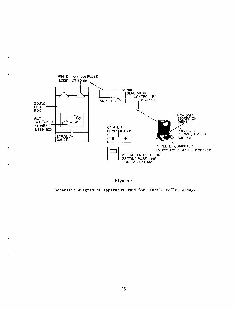
The startle reflex assay tested the time to reaction and the force ofthe response when rats were startled by a sharp auditory stimulus. Ratswere placed in a wire box within a larger sound-insulated box (Fig. 4). Aconstant white noise at 85 dB within the larger box helped eliminateoutside noises. After an acclimation period of 10 min., rats received aseries of five 10 msec pulses of noise at 13,000 Hz and 110 dB separated by25 sec. Their response, or startle reflex, was monitored by a Gould loadcell under the wire box. The entire procedure, including data acquisitionand analysis, was controlled by an Apple microcomputer.

On the basis of pilot work using chlorpromazine and other drugs, itwas decided that the neurotoxicity data could be analyzed best as

24

SOUNDPROOF

BOX

RATCONTAINEDIN WIREMESH BOX

WHITE 10 m sec PULSE

NOISE ATHOdB

SIGNALGENERATOR

CONTROLLEDBY APPLE

RAW DATASTORED ONDISKS

PRINT OUT

OF CALCULATEDVALUES

lZj

APPLE 1+ COMPUTER

EQUPPED WITH A/D CONVERTER

VOLTMETER USED FORSETTING BASE LINEFOR EACH ANIMAL

Figure 4

Schematic diagram of apparatus used for startle reflex assay.

25

differences between pre-exposure and postexposure values for eachindividual. Thus each animal served as its own control.

RESULTS

Aerosol Concentration

In addition to continuous monitoring of the aerosol concentration by

infrared backscatter detectors, filter pad samples of chamber air weredrawn during each exposure for gravimetric analysis of chamber concentration. A summary of the measured and target concentrations is in Table IC(see Appendix C). Mean values for groups exposed to lower concentrationstended to be slightly more than target values while those for the two

groups receiving 6 mg/L were slightly lower than the target. However,actual concentration was generally close to the target concentration; thestudy was therefore conducted in accordance with the experimental design.

Mortality

A Ct product of 8 mg'hr/L had been previously estimated to result in adose of diesel fuel which approximated a maximum tolerated dose, in termsof mortality, and no deaths were seen in the repeated exposures with Ct

products of 0 or 8 mg'hr/L. However, among the groups receiving 12 mg'hr/Lthere was 6.25 percent mortality overall. Eleven rats (10 females and onlyone male) died among the 4 groups receiving this higher exposure. Eight ofthese including the single male fatality were in the group exposed to6 mg/L for 2 hr/exposure at 1 exposure/wk; one death was in each of theother 3 groups. The reason for this apparently unequal distribution ofdeaths is not known.

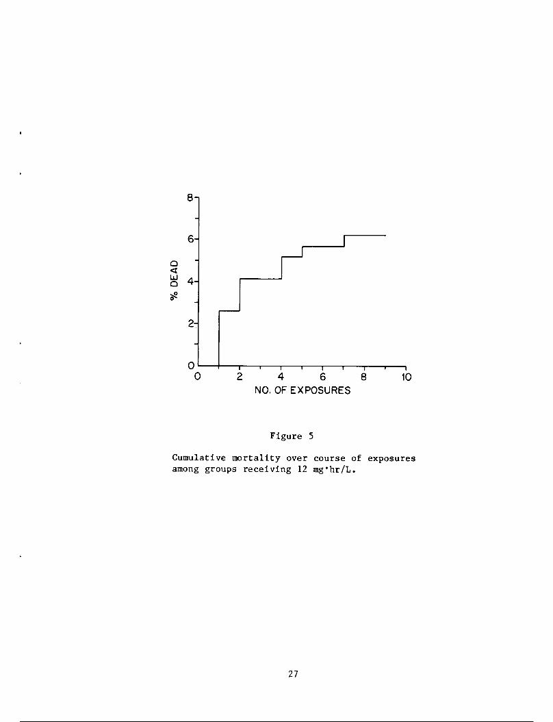
Deaths occurred within 48 hr after a given exposure, as in acuteexposures used to define maximum tolerated exposure conditions. As seen inFigure 5, deaths occurred over the span of 9 exposures, although they weremore frequent during the earlier exposures. At autopsy, lungs wereenlarged and reddened. There occasionally was some fluid in the trachea.No other abnormalities were seen, again giving a picture similar to thatafter acute exposures. It appeared that there was no difference in thecause of death between single and repeated exposures and that the choice of

a Ct product of 8 mg'hr/L for maximal exposure conditions resulting in nosignificant mortality was valid. With exposures to a Ct product 50 percenthigher, significant mortality resulted.

Body Weight

Mean body weights during exposures given once per week or 3 times perweek are shown in Figures 6 and 7 respectively. It is readily apparentfrom these figures that mean body weight was depressed in both sexes byexposure to the aerosol, especially with 3 exposures/week. Weight

26

8-i

6-

Q<

2 4H

2-

—i " 1 1 1 1 1 1 1

0 2 4 6 8 10

NO. OF EXPOSURES

Figure 5

Cumulative mortality over course of exposuresamong groups receiving 12 mg'hr/L.

27

540-1

500-

460-

- 420-

h-IOu 380-

Q

§ 340-

<UJ

300-

260-

220-

MALES

r

/^>y,X^

,0*

^--o-

FEMALES

^-o-

,--°

mg«hr/L 12 8 C

hr/exposure 2 6 2 | 6 2 6

—• --• -+- —0 —0

-1 1 1 1—

12 14 16 18AGE (weeks)

20 22

—i

24

Figure 6

Mean body weight of animals during exposure to aerosolized dieselfuel once per week. Exposures ended after the ninth week.

28

540-1

500-

460-

~ 420-

h-X

S 380-

>-Q

§ 340-

<UJ

300-

260-

220-

MALES

.• ,•

it//o d

\X, o^-Wj\ V

\ -I

FEMALES

-8o^l

•m •--•

—i—

12

mg'hr/L 12 £ C

hr/exposure 2 6 2 6 2 6

—• —• —• —o —0

-1 1—

14 16

AGE (weeks)18

—i

20

Figure 7

Mean body weight of animals during exposure to aerosolized diesel fuel three times per week. Exposuresended after the third week.

29

increased in the groups exposed once per week after an initial depression,the rate of gain being similar to that of sham-exposed controls. After aninitial depression, weight in groups exposed 3 times per week was stablefor the remainder of the exposure period and then rebounded toward controlvalues during the 2 weeks post-exposure.

Weight data were treated statistically by analysis of variance of theweekly weight gains (or loss). Weight gain during the first few weeks ofexposure was affected by all three exposure parameters (exposure, durationof exposure and frequency of exposure). During the first 2 weeks ofexposure, body weight gain was significantly reduced in exposed animalscompared to controls (p = 0.0001 for both sexes). However the extent ofthis difference was not related to Ct product. Frequency of exposure wasalso a significant factor; weight gain among groups exposed once per weekwas greater than it was in those exposed 3 times per week (p = 0.0001 forboth sexes). Groups exposed for 6 hours gained less weight than thoseexposed for 2 hours (p = 0.0001 for both sexes). Least squares mean valuesreflecting these analyses are shown in Tables 2C and 3C. (See Appendix Afor explanation of least squares means.)

Body weights rebounded toward control values after cessation of3-times-per-week exposures (see Fig. 7). Among groups exposed once perweek (Fig. 6), the effect of exposure on rate of weight gain lessened withtime, until there was no significant rebound in weight when exposure wasstopped after nine weeks.

Food Consumption

Weekly food consumption data were obtained for 6 males and 6 femalesin each group throughout the exposure and recovery periods. These valuesare summarized in Figs. 8 and 9. As with body weight, there was an obvioussex difference, and data were analyzed for each sex separately. Nosignificant block effects were observed. And, as with body weight, themost significant effects were seen in the first few weeks of exposure.Food consumption generally decreased significantly with increasing Ctproduct or frequency during the first 3 weeks of exposure, as shown inTables 4C and 5C. No significant relation of duration of exposure anddepression of food consumption was observed.

Food consumption increased in the groups given 3 exposures per weekafter the third week, when those exposures were stopped. In the groupsreceiving 1 exposure per week, there was generally a significant depressionin food consumption for the nine weeks of exposure with no discernablerelation to the Ct product.

Pulmonary Free Cells

The number of alveolar macrophages lavaged from the lungs of allexposed groups at two days post exposure was significantly greater thanthat of controls (p = 0.0001). This increase is evident in the means shown

30

35

33-

31-

~ 29-

o

ao

UJUJ

5

25-

23-

21-

19-

17-

15

MALES

o o'

/ \ ' M

•7WV s^'

FEMALES

oXo—o^

. "Vs

--*• N,-"0

:^*Cxv--'7\/:^,

mg «hr/L

hr/exposure12

2 6 2 I 6

-i 1 r-

2 4 6

—o—o

-i 1

8 10

WEEKS OF TREATMENT

Figure 8

Mean weekly food consumption of animalsduring exposure to aerosolized diesel fuel

once per week. Exposures ended after theninth week.

31

35-i

33-

31-

™ 29H

O

310zoo

QOO

UJUJ

5

27-

25-

23-

21-

19-

17-

15 • . r2 4 6

WEEKS OF TREATMENT

5—/

\ o.

MALES

FEMALES

12 « C

2 6 2 6 2 6

—• --• —• —• —o —o

Figure 9

Mean weekly food consumption of animalsduring exposure to aerosolized diesel

fuel three times per week. Exposuresended after the third week.

32

in Table 6C. There was also a clear sex difference (p = 0.0001) which wasmade essentially insignificant (p = 0.012) by referencing cell number tobody weight. Control values were In the range of 5 x 106 cells/kg for bothsexes. The Increase in cell number was not related to Ct product.Interestingly, the two week period without exposure did not result in asignificant change in the numbers of alveolar macrophages compared tovalues at 2 days post exposure (p = 0.77). This lack of a decrease tocontrol values is also evident in the means in Table 6C. There was nosignificant effect of exposure on cell viability.

The number of lavaged cells other than alveolar macrophages Increasedvery significantly in all groups of exposed animals (p = 0.0001), but againwithout a clear relation to the Ct product. The numbers among exposedgroups were highly variable, as seen in Table 7C. These other cellsconsisted primarily of granulocytes. Differential counts of cells attachedto the coverslips in the yeast assay of 3 groups showed that the percent ofgranulocytes among these "other cells" rose from 2 percent in controlpreparations to 87 percent at 2 days after exposure. Lymphocytes accountedfor 7 percent of these cells and the remaining 6 percent were unidentified.The vast majority of granulocytes appeared to be neutrophils, as waspreviously observed after acute exposures. Unlike the number of macrophages, the number of "other cells" returned essentially to control valuesby 2 weeks without exposure, as seen in Table 7C.

Phagocytic activity of lavaged alveolar macrophages was expressed interms of the number of yeast associated with the cells attached to thecoverslip used in the assay. A typical example of the data from one animalis given in Figure 10. It was found that similar curves from all animalscould be adequately described by a negative binomial distribution whichcould be completely described by Its mean and variance. The mean of thisfrequency distribution is essentially the average number of yeast associatedwith all macrophages examined. This mean is referred to here as thebinding index and is illustrated in Figure 10. Values for binding indexamong the treatment groups are summarized in Table 8C. There were nosignificant changes in binding index which could be related to exposure tothe aerosol.

Pulmonary Function Tests

The results of each pulmonary function test are presented here inessentially the order in which the tests were done. Resistance was thefirst test, representing resistance of the respiratory tract below thetracheal cannula. Values are summarized in Table 9C. No differences inresistance were observed which were related to exposure to the aerosol.However, there was a significant sex-related difference (p = 0.0001).Least squares means were 0.290 ± 0.019 H20/mL/sec for males and0.389 ± 0.019 cm H20/mL/sec for females.

Multibreath nitrogen washout curves were also performed. These can beanalyzed in a variety of ways. All attempt to ascertain how efficientlyN2 present in the lungs is removed or washed out over a series of breaths

33

LUl_

LU

50 -i

40-

£> 30-Orru-oo

fezLU

r->

LUO

rrUJ

o

20-

10-

0 —r

0

V*- Binding Index

==#=

2 4 6

NO. OF YEAST/CELL

8

Figure 10

Percent of macrophages associated with given numberof yeast in phagocytosis assay. Arrow marks bindingindex or average number of yeast associated with amacrophage.

34

of pure O2. One simple method is to express end-tidal N2 concentration interms of breath number when tidal volume Is constant, as illustrated inFigure 11 for males in a control and an exposed group at 2 weekspostexposure. The N„ concentration at the end of exhalation was taken tobest approximate alveolar concentration. In this case it appears that thelungs of the treated group were less well ventilated than those of thecontrols, requiring more breaths to expire the same amount of N2. However,the resting volume of the lung (functional residual capacity or FRC) was3.0 ± 0.2 mL for controls and 3.7 ± 0.2 mL for exposed animals in thisexample. This difference in lung volume must be compensated for incalculations on the washout curves if one is to separate changes inefficiency of ventillation from altered lung volume. In Figure 12 theend-tidal N2 concentration is plotted against the cumulative number oftimes that FRC was diluted by successive breaths. After the elimination ofthe influence of FRC, it is apparent that the two groups do not differ fromone another in this test. The apparent difference noted above was due toincreased resting volume in exposed animals.

All calculations dealing with the nitrogen washout curves were made onthe basis of cumulative dilutions of FRC. One of the analyses performedwas a simple linear regression of the log (percent N2) vs cumulativedilutions of FRC, on the assumption that the lungs washed out exponentiallylike a single compartment. This assumption proved to be nearly true, withcorrelation coefficients generally greater than 0.980. Thus the slope ofthe regression equation was taken as an index of the rate of clearance ofN2 from the lung. These slopes are summarized in Table IOC. The largenumber of standard errors equal to zero is an artifact of rounding. Therewas no exposure-related change in the slope. There was a significant sexdifference, however (p = 0.0001); males had least squares mean slope of-0.188 ± 0.002 while females had a slope of -0.155 ± 0.003. Thus, femaleshad relatively greater resistance to breathing and less rapid washout ofN2 from the lungs.

The number of dilutions required to reach end-tidal concentrations of10 percent and 5 percent nitrogen were also calculated by extrapolationfrom the data points on either side of these nitrogen concentrations foreach animal. Again no exposure-related changes were observed, but therewas a sex difference (p = 0.0001). Least squares mean values for thedilutions to reach 10 percent N2 were 5.19 ± 0.08 for females and4.10 ± 0.08 for males; values for the number of dilutions to reach5 percent N2 were 7.23 ± 0.10 and 5.79 ± 0.10 for females and malesrespectively.

Lung volumes were obtained by combining data from two methods: FRCfrom the Boyle's Law method and a continuum of changes in volume (but notabsolute volumes) ranging from total lung capacity (TLC) to residual volume(RV) from the quaslstatic pressure-volume curve. These two assays werecombined to produce pressure-volume curves of absolute lung volume.Examples of these curves are presented in Figure 13. The lung volumesderived from these curves are shown in the figure, including FRC, TLC, RV,vital capacity (VC), inspiratory capacity (IC), and expiratory reserve

35

1.7 -i

1.5-

1.3-

CM

1.1-

o

0.9-

0.7-

0.5-

-i • 1 " 1 " 1 1 1

3 5 7 9 11

BREATH NO.

Figure 11

Mean multibreath nitrogen washout curves for males ofcontrol group EA (O) and exposed group FA (#). End-tidal N2 concentration is plotted against breathnumber.

36

1.7-i

1.5-

1.3-

CVJ

.o 1.H

0>O

0.9-

0.7-

0.5-

\\

\\

\\

\\V

-I 1 1 r-

2 3 4 5DILUTION OF FRC

-r-

6

Figure 12

Mean multibreath nitrogen washout curves for males of controlgroup EA (O) and exposed group FA (#). End-tidal N2concentration is plotted against cumulative dilutions of FRC.

37

20-1

-30 0 5 10 15 20 25TRANSPULMONARY PRESSURE (cm H20)

30

Figure 13

Quaslstatic pressure-volume curves of lungs from males in control groupHA (O) and exposed group (GA (#). Lung volumes shown are total lungcapacity (TLC), vital capacity (VC), inspiratory capacity (IC),functional residual capacity (FRC), residual volume (RV), and expiratoryreserve volume (ERV).

38

volume (ERV). Changes in these volumes could reflect alterations inarchitectural and/or elastic properties of the lung.

There was some concern that TLC and VC increased significantly withage over the course of exposures since these volumes appeared slightlylower in two control groups assayed at 16 weeks of age than in oldercontrols. In a direct comparison, these two groups (HA and LA) had TLC'slower than the others by about 8 percent. If an age-related increase inlung volume were present, compensation for this change would have to bemade. No such compensation was made for the following reasons:

1) A definite age-related change could not be described over therange of ages in this phase of the toxicologic evaluation ofdiesel fuel aerosols.

2) Groups of exposed animals were exposed over the same range ofages as controls and at approximately the same ages.

3) The youngest groups of exposed animals (aged 15 and 16 weeks)had TLC's in males which were about 14 percent below controlgroups of comparable age, an appreciably greater differencethan the apparent 8 percent noted in controls above.

4) Among female controls in the 6 assays of older controls, therewas as much variation in TLC as there was between those groupscollectively and the two groups assayed at 16 weeks of age.

Values for several lung volumes are presented in Tables 11C-14C.Analysis of the values for TLC showed that it was affected by exposure(p = 0.005), frequency of exposure (p = 0.0001), time postexposure(p = 0.0001), and sex (p = 0.0001). There was also a significantinteraction of exposure and duration of exposure (p = 0.0005). Table 1summarizes the least squares means and standard errors for each of thesevariables. Definitions of terms used in this and subsequent tables aregiven in Appendix C.

39

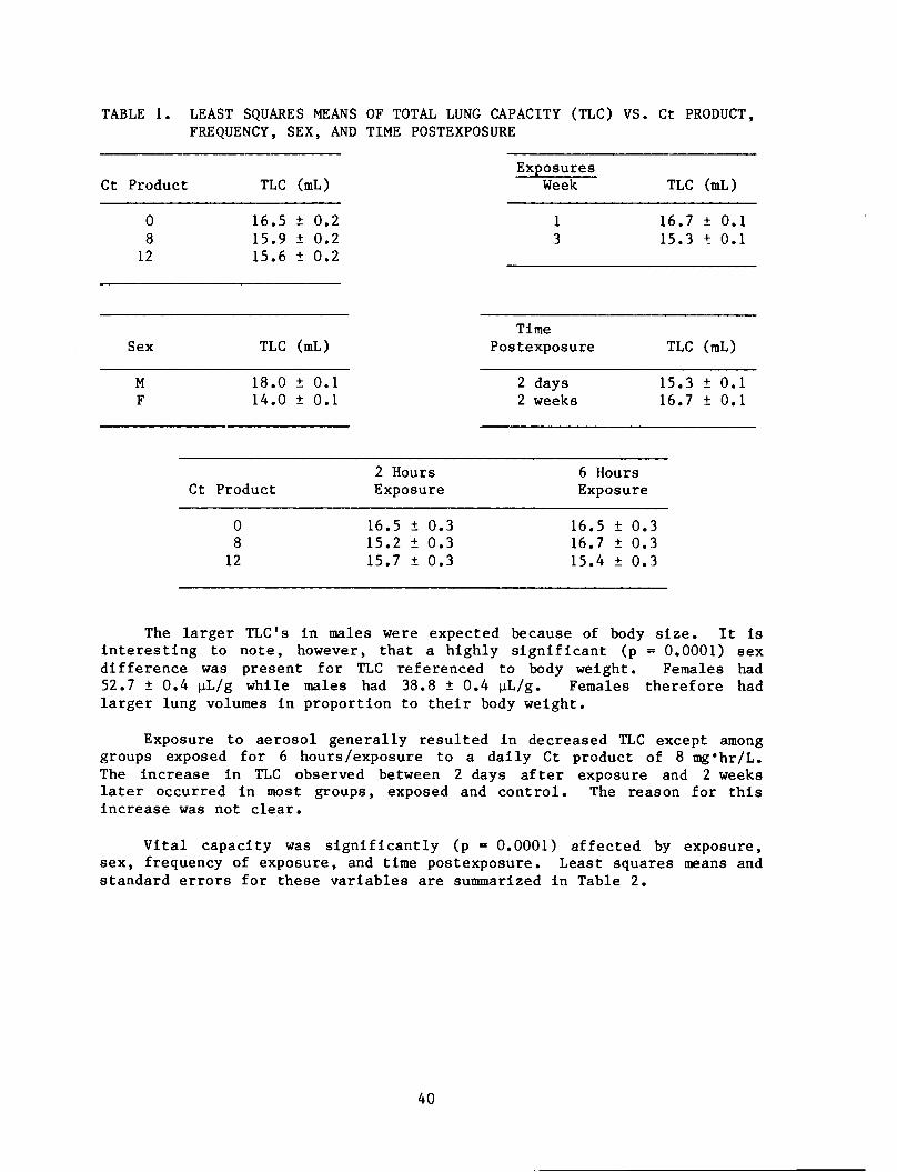
TABLE 1. LEAST SQUARES MEANS OF TOTAL LUNG CAPACITY (TLC) VS. Ct PRODUCT,FREQUENCY, SEX, AND TIME POSTEXPOSURE

Ct Product TLC (mL)Exposures

Week TLC (mL)

0

8

12

16.5

15.9

15.6

± 0.2

± 0.2

± 0.2

1

3

16.7

15.3

± 0.1

± 0.1

Sex TLC (mL)Time

Postexposure TLC (mL)

M

F

18.0

14.0

± 0.1

± 0.1

2 days2 weeks

15.3

16.7

± 0.1

± 0.1

Ct Product

2 Hours

Exposure1

6 Hours

Exposurei

0

8

12

16,

15,

15,

.5

.2

.7

+

+

+

0.

0.

0.

,3

,3

,3

16.5

16.7

15.4

+

+

+

0.

0.

0.

,3

,3

,3

The larger TLC's in males were expected because of body size. It isinteresting to note, however, that a highly significant (p = 0.0001) sexdifference was present for TLC referenced to body weight. Females had52.7 ± 0.4 uL/g while males had 38.8 ± 0.4 uL/g. Females therefore hadlarger lung volumes in proportion to their body weight.

Exposure to aerosol generally resulted in decreased TLC except amonggroups exposed for 6 hours/exposure to a daily Ct product of 8 mg'hr/L.The increase in TLC observed between 2 days after exposure and 2 weekslater occurred in most groups, exposed and control. The reason for thisincrease was not clear.

Vital capacity was significantly (p = 0.0001) affected by exposure,sex, frequency of exposure, and time postexposure. Least squares means andstandard errors for these variables are summarized in Table 2.

40

TABLE 2. LEAST SQUARES MEANS OF VITAL CAPACITY (VC) VS. Ct PRODUCTFREQUENCY, SEX, AND TIME POSTEXPOSURE

Ct Product VC (mL)

0 14.3 ± 0.2

8 13.6 ± 0.2

12 12.9 ± 0.2

Sex

M

F

VC (mL)

15.3 ± 0.1

11.9 ± 0.1

ExposuresWeek VC (mL)

1

3

14.2 ± 0.1

13.0 ± 0.1

Time

Postexposure VC (mL)

2 days2 weeks

13.1 ± 0.1

14.1 ± 0.1

As with TLC, females had proportionately higher VC's for their body weightthan did males (44.7 ± 0.4 vs 32.9 ± 0.3 uL/g). Vital capacity changesfollowed those for TLC except that the exposure-time interaction wasmarginally significant (p = 0.04). Least squares means for this interactionare given in Table 3.

TABLE 3. INTERACTION OF VITAL CAPACITY Ct PRODUCT ANDTIME POSTEXPOSURE

Ct Product

0

8

12

2 Hours

Exposure

14.2 ± 0.2

13.1 ± 0.2

13.0 ± 0.2

6 Hours

Exposure

14.4 ± 0.2

14.0 ± 0.2

12.9 ± 0.2

The pattern for inspiratory capacity was very similar, with significant(p = 0.0001) effects of exposure, sex, frequency of exposure, and time afterlast exposure. The exposure-duration interaction was marginal (p = 0.016).Again, least squares means are given in Table 4.

41

TABLE 4. LEAST SQUARES MEANS OF INSPIRATORY CAPACITY (IC) VS. Ct PRODUCT,FREQUENCY, SEX, AND TIME POSTEXPOSURE

Ct Product IC (mL)

0 13.4 ± 0.2

8 12.5 ± 0.2

2 12.0 ± 0.2

Sex

M

F

IC (mL)

14.2 ±

11.1 ±

Ct Product

0

8

12

0.1

0.1

2 Hours

Exposure

13.3 ± 0.2

12.0 ± 0.2

12.0 ± 0.2

ExposuresWeek IC (mL)

1

3

13.1 ± 0.1

12.1 ± 0.1

Time

Postexposure IC (mL)

2 days2 weeks

12.1 ± 0.1

13.1 ± 0.1

6 Hours

Exposure

13.4 ± 0.2

13.1 ± 0.2

12.0 ± 0.2

Rather than decreasing with exposure, FRC significantly (p = 0.0001)increased by 9 percent among groups receiving 8 mg'hr/L and 15 percentafter exposure to 12 mg'hr/L. There were also significant (p = 0.0001)effects of sex, frequency of exposure, time after exposure, and interactionof exposure and time. Animals exposed over a longer time (1/wk) had largervalues (by 13 percent) for FRC which also increased during the 2 weekpostexposure period. In the exposure-time interaction, the effect wasreversed from that of previous lung volumes; FRC increased among groupsreceiving 12 mg'hr/L and only in those having 6 hour exposures with8 mg'hr/L. Least squares means and standard errors are given in Table 5.

42

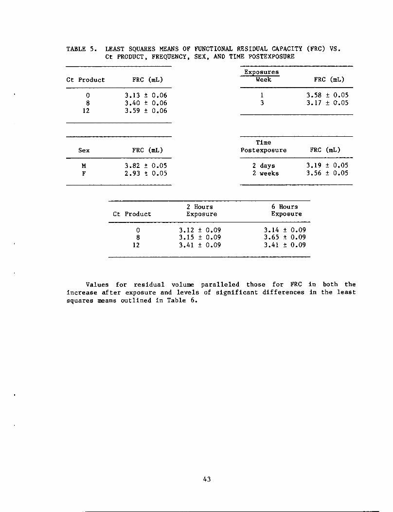
TABLE 5. LEAST SQUARES MEANS OF FUNCTIONAL RESIDUAL CAPACITY (FRC) VS.Ct PRODUCT, FREQUENCY, SEX, AND TIME POSTEXPOSURE

Ct Product

0

8

12

Sex

M

F

FRC (mL)

3.13 ± 0.06

3.40 ± 0.06

3.59 ± 0.06

FRC (mL)

3.82 ±

2.93 ±

0.05

0.05

Ct Product

0

8

12

2 Hours

Exposure

3.12 ± 0.09

3.15 ± 0.09

3.41 ± 0.09

ExposuresWeek FRC (mL)

1

3

3.58 ± 0.05

3.17 ± O.05

Time

Postexposure FRC (mL)

2 days2 weeks

3.19 ± 0.05

3.56 ± 0.05

6 Hours

Exposure

3.14 ± 0.09

3.65 ± 0.09

3.41 ± 0.09

Values for residual volume paralleled those for FRC in both theincrease after exposure and levels of significant differences in the leastsquares means outlined in Table 6.

43

TABLE 6. LEAST SQUARES MEANSFREQUENCY, SEX, AND

OF RESIDUAL

TIME POSTEXI

VOLUME (RV) VS. <'OSURE

Zt PROCUCT,

Ct Product RV (mL)Exposures

Week RV (mL)

0

8

12

2.22

2.39

2.65

± 0.06

± 0.06

± 0.06

1

3

2.54 ± 0.04

2.30 ± 0.04

Sex RV (mL)Time

Postexposure Rv (mL)

M

F

2.74

2.10

± 0.04

± 0.04

2 days2 weeks

2.25 ± 0.04

2.59 ± 0.04

Ct Product

2 Hours

Exposurei

6 Hours

Exposure

0

8

12

2.28

2.09

2.73

± 0.

± 0.

± 0.

,07

,07

,08

2.16 ±

2.69 ±

2.57 ±

0.

0.

0.

,07

,08

,08

All lung volumes discussed thus far were derived from the combinationof values for FRC and the quaslstatic pressure-volume curves. Another wayof analyzing the pressure-volume curves is in terms of compliance, theslope of the pressure-volume curve over a specified range of transpulmonarypressure. Compliance differs at various locations along the curve and withchanges in lung site. A specific pressure range is used to define thelocation on the curve being examined. To help compensate for variations inlung volume, the compliance value may be divided by actual lung volume atthe midrange of the chosen transpulmonary pressures to yield a numbercalled specific compliance. The specific compliance values given inTable 15C are the changes In lung volume from transpulmonary pressures of 0to 10 cm H20 divided by lung volume at 5 cm H20.

Analysis of least squares means for specific compliance revealedsignificant effects of exposure (p = 0.0001), frequency of exposure(p = 0.0001), sex (p = 0.007), and interaction of exposure and duration ofeach exposure (p = 0.005). Least squares means (± S.E.) for these variablesare in Table 7.

44

TABLE 7. LEAST SQUARES MEANS OF SPECIFIC COMPLIANCE (C8D) VS. Ct PRODUCT,FREQUENCY, SEX, AND TIME POSTEXPOSURE

Ct Product

mg'hr/L cspExposures

Week csp

0

8

12

1.15 ± 0.01

1.04 ± 0.01

0.97 ± 0.01

1

3

1.02 ± 0.01

1.09 ± 0.01

Ct product

mg'hr/L 2 hrs/

C8p

'exposureSex c,sp 6 hrs/exposure

M 1.03

F 1.08

+

+

0.

0.

.01

.01

0

8

12

1.16

1.08

0.95

± 0.02

± 0.02

± 0.02

1.14 ± 0.02

1.00 ± 0.02

0.99 + 0.02

As one would expect from the data on lung volumes, specific compliancedecreased with exposure and was lower in animals exposed once per week.Values for females were higher than those for males.

The maximal forced exhalation maneuver was used to test for functionalobstruction of the airways. In this assay, the animals were made to inhaleto TLC and then forced to exhale under conditions such that theirrespiratory system limited the maximum flow achieved at any given lungvolume. Expiratory flow was analyzed in terms of peak flow, flow at50 percent of vital capacity, and flow when 25 percent of vital capacityremained. Means of the original flows at these specific lung volumes arein Tables 16C-18C. There appeared to be a decrease in maximal flow amongthe groups receiving the highest Ct product and more frequent exposures.However, vital capacity was also decreased among these groups. Sincemaximal flow is related to vital capacity, the question arose as to whetherthe apparent effect of exposure on maximal flows was a result of decreasedVC. As seen in Table 19C, maximal flow at 50 percent of VC was notaffected by exposure when the size of the lungs was accounted for byreferencing flow to VC. A plot of peak flow against vital capacity led tothe same conclusion. Therefore no evidence for functional obstruction ofthe airways was observed in this assay.

The rate of diffusion of carbon monoxide from the lung was used as anindex of the efficiency of gas exchange across the lung. Values from thesingle-breath maneuver, in mL/(mmHg) (min), are summarized in Table 20C.Significant (p = 0.0001) effects were observed for sex, exposure, dose-time,and dose-frequency. However, the absolute value for diffusing capacitywould be related to lung size; larger lungs should have larger diffusingcapacities. Therefore diffusing capacity was referenced to total lungcapacity (in liters), as summarized in Table 21C. Significant effects

45

(p = 0.0001) were again found for sex, exposure, dose-time, and dose-frequency. Least squares means are shown below in Table 8.

TABLE 8. LEAST SQUARES MEANS OF DIFFUSING CAPACITY AND DIFFUSINGCAPACITY/TLC (IN LITERS) VS. Ct PRODUCT, SEX, AND FREQUENCY

Diffusing Capacity Diffusing Capacity/TLC

Ct (mg'hr/L)

0 0.964 ± 0.018

8 0.899

12 0.769

57.6 ± 1.0

55.4

48.5

Diffusing Capacity Diffusing Capacity/TLC

Sex

M

F

1.108 ± 0.014

0.647

61.6 ± 0.8

46.1

Diffuising Capacity Diffusing Capacity/TLC

Frequency Frequency

Ct 1/wk 3/wk 1/wk 3/wk

0

8

12

0.939

0.969

0.876

0.989 ± 0.025

0.829

0.663

54.7 60.5 ± 1.9

57.1 53.7

52.3 44.7

Although there was not a consistent exposure-related decrease in COdiffusion, the low values were among the groups receiving 3 exposures/weekand especially those at the higher exposure level (See Tables 20C and 21C).

Organ Weights

Wet weights were taken on the right middle lung lobe, liver, leftkidney, and left adrenal gland. Mean weights for the liver, kidney, andadrenal are in Tables 22C, 23C, and 24C, respectively. As expected, liverweight was greater in males than in females (p = 0.0001, 15.3 ± 0.1 and9.0 ± 0.1, respectively) and weight tended to increase with age. Overall,there was a decrease in least squares means related to exposure (p = 0.0001).

46

Mean weight in controls (both sexes combined) was 12.74 ± 0.16 g, 11.74 ±0.16 g in groups given 8 mg'hr/L, and 11.90 ± 0.16 g in groups given12 mg'hr/L.

Kidney weight was also lower in females than in males (p = 0.0001,0.96 ± 0.01 g vs 1.61 ± 0.01 g, respectively) and tended to increase withage. However, there was not an exposure-related change in mean weights.As is evident in Table 24C, adrenal weight was greater in females(p = 0.0001; 33.6 ± 0.4 mg in females and 28.0 ± 0.4 mg in males).Although exposure to diesel fuel itself did not influence adrenal weight\there was a small but significant Increase (p = 0.0001) among groupsexposed 3 times per week (31.9 ± 0.4 mg) over those exposed once per week(29.7 ± 0.4 mg). Adrenal weight did not change with age. This effect offrequency of exposures thus did not appear to be related to the diesel fuelbut more to the stress of handling during exposure.

Wet weight of the right middle lobe also did not change with age ineither sex; but there was an increase positively correlated with exposureto diesel fuel (p = 0.0001), as seen in Table 25C. Lobes from males had ahigher (p = 0.0001) weight than those from females (202 ± 2 mg and152 ± 2 mg, respectively). The mean weights from both sexes togetherincreased with the Ct product when examined at both 2 days and 2 weekspostexposure. However, the weights of lobes taken from exposed animals2 weeks postexposure were significantly lower than those of lobes taken2 days postexposure, as seen in Table 25C of the raw data and the leastsquares means shown in Table 9.

TABLE 9. LEAST SQUARES MEANS OF WEIGHT OF RIGHT MIDDLE LUNG LOBE VS.Ct PRODUCT AND RECOVERY PERIOD

Timemg'hr/L

Postexposure 0 8 12

2 days 152 ±3 188 ± 3 213 ± 32 weeks 156 ±3 172+3 181+3

Even though wet weight was increased by exposure, the wet to dry ratioof lung weight was not significantly changed. As seen in Table 26C, thisratio remained constant at just over a value of 5 in most groups. ' Thisconsistancy in the wet to dry ratio indicated that the wet weight increasesprobably were predominantly cellular rather than from edema.

47

Histopathology

The lung was the only organ examined histologically that consistentlyhad lesions which could be related to diesel fuel exposure. There were noexposure-related lesions observed in the remainder of the respiratory tractor in any of the other organs examined. Control animals had occasionalareas of focal pneumonitis, consisting of local accumulations of inflammatory cells within the alveoli, and peribronchial and perivascular inflammatory lesions. Since the lesions in exposed animals were quite similar inappearance to those in controls, care was taken to discriminate betweenthem. Lesions observed after diesel fuel exposure were generally focalaccumulations of alveolar macrophages and other free cells in the alveoliand associated thickening of the alveolar wall with hypercellularity(probably lymphocytes and hlstocytes). The presence of septal fibrosiscould not be determined on the H&E slides routinely prepared.

A summary of individual observations is given in Appendix D. Groupsummaries of the severity of pulmonary lesions are shown in Table 27C. Thescoring method was standardized by the pathologist and was based on the relative numbers of alveolar free cells and the hypercellularity of the alveolarwalls. As seen in the table, there was some overlap between control andexposed groups with some exposed animals having essentially normal lungs.It should be emphasized, however, that only one section of the lung wastaken. This section cannot be taken as being necessarily representative ofthe focal lesions potentially distributed throughout the lungs.

The animals exposed to a Ct product of 12 mg'hr/L had generally higherscores using the scoring scheme described above than those of groupsexposed to 8 mg'hr/L. Those examined at 2 weeks after exposure had feweralveolar free cells (as seen in Table 7C) but more cellularlty of thealveolar walls, with a possible slight increase in the number of interstitial cells. Large numbers of free cells still remained in the alveoli.Rupture of alveolar walls was most common in groups GA (6 mg/L, 2 hr/exposure, 3 exposures/wk) and CA (2 mg/L, 6 hr/exposure, 3 exposures/wk),the two groups exposed to a CT product of 12 at the higher exposurefrequency. Rupture was also noted in one animal each from groups DA(4 mg/L, 2 hr/exposure, 3 exposures/wk) and HA (control).

The control group HA also had a high incidence of liver and kidneyalterations which were not observed among exposed animals (see Appendix D).These lesions were mild and were observed only among those animals killedat 2 days postexposure. They could not be related to housing conditions (orany other known factor) and appeared to be a random incidence of normallesions observed in these animals. No histopathologic reason for thedecrease in liver weight among exposed animals was observed.

Neurotoxicity

No significant alterations, which could be related to diesel fuelexposure, were observed in any of the four neurotoxicity assays. In eachassay, pre-exposure values served as baseline data. Observations made at

48

one day or two weeks after the last exposure were related to thesepretreatment values for each Individual, and the changes in a givenparameter for each individual animal were analyzed statistically. Thus,each animal served as its own control.

Pre-exposure means for forelimb grip strength appear In Table 28C. Itis apparent from the table that males had higher values. And analysis ofleast squares means revealed a significant difference (0.97 ± 0.02 kg formales and 0.84 ± 0.02 kg for females, p = 0.0001). No exposure-relatedchanges from the pre-treatment values were observed at 1 day or 2 weeksafter the last exposure. The magnitudes of the observed decreases aresummarized in Table 10.

TABLE 10. LEAST SQUARES MEANS OF CHANGE FROM PRE-EXPOSUREVALUE OF FORELIMB GRIP STRENGTH VS. Ct PRODUCT

AND TIME POSTEXPOSURE

Ct Product

mg'hr/L

0

8

12

1 DayPostexposure

-0.02 ± 0.03

-0.09 ± 0.03

-0.07 ± 0.03

2 Weeks

Postexposure

-0.04 ± 0.04

-0.07 + 0.04

-0.13 ± 0.04

Pre-exposure means for landing foot spread are shown in Table 29C.Males again had significantly greater values (114 ± 2 min vs 92 ± 2 min,p = 0.0001) than females and there were no significant changes related toexposure. Least squares means of the differences between pre-exposure andpostexposure values are illustrated in Table 11.

TABLE 11. LEAST SQUARES MEANS OF CHANGE FROM PRE-EXPOSUREVALUE OF LANDING FOOT SPREAD VS. Ct PRODUCT AND

TIME POSTEXPOSURE

Ct Product

mg'hr/L

0

8

12

1 Day

Postexposure

8.0 ± 3.3

-1.2 ± 3.3

3.9 + 3.4

2 Weeks

Postexposure

6.0 ± 3.3

1.2 ± 3.3

3.2 ± 3.3

Pre-exposure values for tall flick are in Table 30C. Males reactedmore slowly than females with tail flick times of 1.73 ± 0.04 sec and1.53 ± 0.04 sec respectively (p = 0.001). There was a significantexposure-related decrease at 1 day after the last exposure (p = 0.0003),

49

but this effect was not present two weeks later. If the effect was real,it was only transient in nature. The least squares means of the changes intail flick time are shown in Table 12.

TABLE 12. LEAST SQUARES MEANS OF CHANGE FROM PRE-EXPOSUREVALUE OF TAIL FLICK VS. Ct PRODUCT AND TIME

POSTEXPOSURE

Ct Product 1 Day 2 Weeksmg'hr/L Postexposure Postexposure

0 0.02 ± 0.07 -0.11 ± 0.088 -0.40 ± 0.07 -0.26 ± 0.0812 -0.13 ± 0.07 -0.10 ± 0.08

Three types of data were derived from the startle reflex assay:reaction time (msec from the sound stimulus to start of response), peaktime (msec from stimulus to maximal response), and peak height (magnitudeof maximum reaction). Pre-exposure values for each are presented inTables 31C-33C. There was a significant sex difference for each (p = 0.0065for peak time and p = 0.0001 for reaction time and peak height). As couldbe expected, the peak height was greater In males than in females (leastsquares means of 357 ± 14 and 246 ± 15 g. wt., respectively). Reactiontime was slightly longer in males (17.9 ± 0.1 vs 17.3 ± 0.1 msec), as waspeak time (27.3 ± 0.3 vs 26.3 ± 0.3 msec). A significant block effect(p = 0.001) was observed only with peak height and this effect wascompensated for in the statistical analysis.

At one day and at two weeks after the last exposure, reaction time andpeak time were not significantly effected by exposure. The initial leastsquares means and differences between postexposure and pre-exposure valuesare given in Tables 13 and 14.

TABLE 13. PRE-EXPOSURE MEANS AND POSTEXPOSURE DIFFERENCES IN REACTIONTIME IN THE STARTLE REFLEX ASSAY (LEAST SQUARES MEANS)

— «

Ct Product Pre-exposure Mean

(msec)

Postexpos ure Difference

mg'hr/L 1 Day 2 Weeks

0

8

12

17.7 ± 0.2

17.5 ± 0.2

17.6 ± 0.2

0.4 ± 0.3

-0.2 ± 0.3

0.1 ± 0.3

-0.5 ± 0.2

-0.2 ± 0.2

-0.2 ± 0.2

50

TABLE 14. PRE-EXPOSURE MEANS AND POSTEXPOSURE DIFFERENCES IN PEAK

TIME IN THE STARTLE REFLEX ASSAY (LEAST SQUARES MEANS)

Ct Product

mg'hr/LPre-exposure Mean

(msec)

Postexposure Difference

1 Day 2 Weeks

0

8

12

26.7 ± 0.4

26.5 ± 0.4

27.1 ± 0.4

1.0 ± 0.5

0.1 ± 0.5

0.5 ± 0.5

0.6 ± 0.5

0.3 ± 0.5

0.6 ± 0.5

Unlike pre-exposure reaction time and peak time, pre-exposure valuesfor peak height were slightly affected by dose group (p = 0.014) (seeTable 15).

TABLE 15. PRE-EXPOSURE MEANS AND POSTEXPOSURE DIFFERENCES IN PEAK

HEIGHT IN THE STARTLE REFLEX ASSAY (LEAST SQUARES MEANS)

Ct Product

mg'hr/L

0

8

12

Pre-exposure Mean

347 ± 20

263 ± 20

294 ± 20

Postexposure Differences

1 Day

61 ± 21

127 ± 21

90 ± 21

2 Weeks

52 ± 22

114 ± 22

97 ± 22

Those groups with lower initial heights tended to have greater increases byone day postexposure, giving overall postexposure means within a relativelynarrow range of 377 to 408 g. wt. Although there were not significantdifferences among the treatment groups in the height increases, it appearedas though initial variability among the groups decreased with age as the

peak heights moved toward a common value of about 390 g. wt. regardless ofaerosol exposure. Referencing values to body weight or age did not resultin exposure-related differences for any of the neurotoxicity assays.

Clinical Chemistry

Both red and white blood cell counts were performed in addition toclinical chemistry on serum samples. There was a significant (p = 0.0001)block effect in RBC numbers. After compensation for the block effect,there still were significant effects of exposure and frequency of exposure(p = 0.001). The interaction of these two factors is demonstrated inTable 16.

51

TABLE 16. LEAST SQUARES MEANS OF RED BLOOD CELL COUNT VS. Ct PRODUCTAND FREQUENCY

Exposures/WeekCt Product

mg'hr/L 1 3

0 4.87 ± 0.10 5.09 ± 0.10

8 5.06 ± 0.10 4.32 ± 0.10

12 4.72 ± 0.13 4.30 ± 0.10

The number of RBC's was decreased among groups exposed 3 times/week but notamong those exposed once weekly.

Changes in WBC number resulting from exposure were not as clear.Males had higher counts (3.79 ± 0.12 vs 1.78 ± 0.13 WBC x 103/mm3 infemales, p = 0.0001). Those groups exposed 3 times/week had higher countsthan those exposed once weekly (3.08 ± 0.12 vs 2.49 ± 0.13 WBC x 103/mm3,p = 0.0001). But the effect of exposure was marginal (p = 0.032). Leastsquares means were 3.13 ± 0.16 for controls, 2.54 ± 0.16 for a Ct productof 8 mg.hr/L, and 2.68 ± 0.19 for a Ct product of 12 mg.hr/L. Therefore,there was only a tendency for exposure to result in lower WBC counts.

A variety of clinical chemistry assays were performed on serum samples.These samples were frozen shortly after collection and assayed within4 days. Dr. Carl Burtis of ORNL's clinical chemistry laboratory statedthat only LDH values would be affected by this procedure (compared withfresh serum samples). Very little was observed which could be related todiesel fuel exposures. Therefore, only least square means for sham-exposedcontrols are presented in Table 34C to provide an idea of the data obtained.Alkaline phosphatase activity and concentrations of triglyceride and sodiumwere the only blood chemistry measurements that were affected significantlyby diesel fuel exposure.

Alkaline phosphatase activity increased in exposed animals but only infemales and with marginal statistical significance (p = 0.03), asillustrated in Table 17.

TABLE 17. LEAST SQUARES MEANS OF ALKALINEPHOSPHATASE ACTIVITY VS. Ct PRODUCT

Ct Product

mg'hr/L Males Females

0 150 ± 7 108 ± 7

8 139 ± 7 135 ± 7

12 154 ±7 148 ± 10

52

After consideration of the variability apparent from the standard errors,this increase can be considered slight. The increase in sodium concentration was also small (144.8 ± 0.3 In controls to 147.4 ± 0.3 in exposedgroups) but significant (p = 0.0001). Triglyceride levels were alsodirectly affected by exposure (p = 0.005), decreasing after exposure from123.2 ± 5.1 for Ct = 0 to 80.0 ± 5.0 for Ct = 8 and 79.2 ± 6.0 for Ct =12 mg'hr/L. The effect appeared to be transient; triglyceride rosesignificantly (p = 0.0001) from 82.0 ± 3.7 mg percent at 2 days after thelast exposure to 106.3 ± 4.3 mg percent two weeks later. This pattern ofexposure-related change In triglyceride was similar to those of body weightand food consumption and may be related to them.

DISCUSSION

The overall objective of this study, the second of three phases ofwhich is reported here, was to determine the biologic effects of exposureto variations in aerosol concentration, duration of each exposure, andfrequency of exposures. During a series of single acute exposures (thefirst phase of the study), mortality was observed to be highly related tothe Ct product (2). Therefore, the Ct product was used in this study as aconvenient parameter for setting exposure conditions. The primaryobjective of the study, however, was not to investigate the relation of theCt product to given endpoints, but the relation of time, concentration, andfrequency to those endpoints. Elucidation of a "dose"-response in terms ofthe Ct product was considered a secondary objective and no presumption wasmade on the linearity of a Ct-response curve.

The combinations of exposure durations and concentrations used inPhase 2 were based on mortality data from the acute exposures. Initially,a Ct-product of 8 mg'hr/L was estimated to be the lower confidence boundfor LCtQi in acute exposures of Phase 1, and therefore, a maximum toleratedexposure level for repeated exposures in Phase 2. However, after a seriesof preliminary exposures with a Ct of 8 mg'hr/L as a maximal "dose", it wasdecided to start exposures again with 12 mg'hr/L as an upper limit, eventhough there was a significant likelihood of deaths as a result of thehigher exposure level. This decision was based on the lack of highlysignificant effects from the initial series of exposures with 8 mg'hr/L.Mortality from the subsequent repeated exposures to 8 and 12 mg'hr/Lapproximated that expected on the basis of acute exposures. About6 percent of the animals receiving the higher exposure level (12 mg'hr/L)died, while there were no deaths with 8 mg'hr/L.

Body weight was also affected by exposure to the aerosol, particularlyamong the groups exposed 3 times per week in which mean weights weredepressed over the entire 3 weeks of exposure. Depressions in foodconsumption generally paralleled those in body weight. To help place theexposure conditions into perspective, exposures three times per week to Ctproducts of 8 or 12 mg'h/L caused a depression in body weight approximately10 percent below that of controls. A maximum tolerated dose can be definedas a dose (Ct product) which produces less than a 10 percent depression in

53

body weight. In addition, approximately 6 percent of animals exposed to12 mg'hr/L died; a maximum tolerated dose should result in no deaths. Byeither criteria, body weight or mortality, the exposure regimen used inPhase 2 resulted in effective doses of diesel fuel which could not havebeen increased without quite deleterious effects.

Of the organs examined, the lungs were most significantly affected byexposure. The small particle size (mass median diameter of about 1 um)probably favored aerosol deposition in the lung rather than upper airways.Thus no effects were observed in the airways histologically or in pulmonaryfunction tests associated with abnormalities in the airways. In the lungparenchyma, however, there was histologic evidence of generally focalaccumulations of alveolar macrophages and other free cells in the alveolialong with associated thickening of the alveolar wall with hypercellularity.Those groups exposed to 12 mg'hr/L generally had the most severe lesionsand, during the two-week postexposure period, the number of free alveolarcells decreased while the cellularity of the alveolar walls worsened.

The number of lavaged pulmonary free cells correlated well withhistologic observations. The number of macrophages and other cells,predominantly neutrophils, was increased greatly in lavages at 2 dayspostexposure. After two subsequent weeks with no exposures, the numberof macrophages remained elevated while the number of other free cells

returned to control values. These observations appeared to reflect apersistent effect of the aerosol.

Additional evidence of changes in the lung parenchyma was seen inthe pulmonary function tests. Carbon monoxide diffusing capacity wasdecreased in several exposed groups at both two days and two weeks afterexposure, reflecting an impairment in gas diffusion from the lung toblood. Also, exposed groups usually showed changes in lung volumesincluding increased functional residual capacity (FRC) and decreasedtotal lung capacity (TLC) and vital capacity (VC). These changes wereaccompanied by a decrease in specific lung compliance at low lungvolumes.

FRC and TLC were most affected in groups CA and GA (12 mg'hr/L,3 exposures/wk) and DA (8 mg'hr/L, 3 exposures/wk), as seen in thetables of results. Although the amount of histopathological examinationof the lungs was limited to one slide per animal, it is interesting tonote that alveolar rupture was noted most commonly in these groups,particuarly CA and GA. A decreased vital capacity, increased FRC andobservable alveolar ruptures indicated the possibility of significantdamage to the architecture of the lung parenchyma. Morphometric analysisof the lung could provide a quantitative correlation to the physiologic andmore subjective histopathologic changes observed. However, it is very timeconsuming and tedious. Therefore, a limited amount of morphometry wasperformed on lungs of males from four groups, although it was not originallyplanned. The paraffin sections were examined at a magnification of 250Xwith a Weibel reticule and the mean linear intercept (Lm) in alveolarparenchyma determined. Results are given in Table 18.

54

TABLE 18. MEAN LINEAR INTERCEPT AND FUNCTIONAL RESIDUAL CAPACITY

Group mg

Hours

ExposureExposures

Week FRC (mL) Lm (um)

EA 0 2 1 3.0 105 ± 3

LA 0 2 3 3.7 102 ± 3

FA 2 6 1 3.7 190 ± 5

CA 2 6 3 4.9 116 ± 5

Although these data are extremely limited, it would seem that there is arelationship between alveolar rupture and mean linear intercept.Furthermore, although not reflected in this table, there appears to be acorrelation between Ct, the amount of alveolar rupture observed, andFRC.

The increase in pulmonary free cell number was expected to occur afternine exposures. But the extent of changes in lung volumes was rathersurprising. Whether these changes observed in the lung would resolve withadditional time is not known; but there is the potential for essentiallypermanent damage to the lung.

There were more systemic changes observed in exposed animals otherthan those in the lung. Liver weight was decreased even though no abnormalities were observed histologically. The number of circulating red bloodcells decreased by about 13 percent among groups exposed 3 times per week,but not in groups exposed once per week. The concentration of sodium inthe serum of exposed groups increased by about 2 percent. And there was atransient decrease in serum triglyceride which seemed to parallel changesin body weight and food consumption. Of these observations, only thealtered triglyceride levels could be related to other exposure-relatedchanges.

None of these systemic changes can be considered of great biologicsignificance at this point. Liver weight, triglceride level and foodconsumption may be related to each other and reflect the stress of exposure.The change In serum sodium, a 2 percent increase, was statisticallysignificant only because the variance for this parameter is normally verysmall. The decrease In circulating RBC's, although observed only with thehigher frequency exposures, indicated a possibly significant impairmentwhich should be monitored closely in future experiments.

In regard to the original objective of this study concerning therelative importance of concentration, duration of exposure, andfrequency of exposures, it was frequency which appeared as the dominantvariable over the range of parameters used in this study. Duration (2

55

or 6 hrs) appeared to have very little effect and a "dose"-response wasoften not apparent with differences in concentration.

56

LITERATURE CITED

1. MacFarland, H. N. 1976. Respiratory toxicology. In Essays InToxicology, Vol. 7, W. J. Hayes, Jr., ed., pp 121-153. AcademicPress, NY

2. Dalbey, W., and S. Lock. 1982. Inhalation Toxicology of DieselFuel Obscurant Aerosol in Sprague-Dawley Rats. Final Report,Phase 1, Acute Exposures. Army Project Orders No 9600 and 0027.Oak Ridge National Laboratory, Oak Ridge, TN. AD A132650.

3. Dalbey, W. E., S. Lock, R. Holmberg, J. H. Moneyhun, R. A. Jenkins,and M. R. Guerin. 1981. Toxicologic evaluation of an aerosol ofdiesel fuel #2. In Proceedings of the 11th Conference onEnvironmental Toxicology, Wright-Patterson Air Force Base, Dayton,OH, November, 1980. pp 220-231, AFAMRL-TR-80-125.

4. Amdur, M. 0., and J. Mead. 1958. Mechanics of respiration inunanesthetized guinea pigs. Amer. J. Physiol. 192: 364-368.

5. Raub, J. A., R. R. Mercer, F. J. Miller, J. A. Graham, and J. J.O'Neil. 1982. Dose response of elastase-induced emphysema inhamsters. Am. Rev. Resp. Dis. 125: 432-435.

6. Lai, Y.-L., and J. Hildebrandt. 1978. Respiratory mechanics in theanesthetized rat. J. Appl. Physiol. 45: 255-260.

7. Diamond, L., and M. O'Donnell. 1977. Pulmonary mechanics in normalrats. J. Appl. Physiol. 43: 942-948.

8. Comroe, J. H., R. E. Forster, A. B. DuBois, W. A. Briscoe, andE. Carlsen. 1962. The Lung. Clinical Physiology and PulmonaryFunction Tests. Yearbook Medical Publishers, Chicago.

9. Jolicoeur, F. B., D. B. Rondeau, A. Barbeau, and M. J. Wagner.1979. Comparison of neurobehavioral effects induced by variousexperimental models of ataxia in the rat. Meurobehav. Toxicol. 1(Suppl. 1): 175-178.

10. D'Amour, F. E., and D. L. Smith. 1941. A method for determiningloss of pain sensation. J. Pharmacol. Exp. Ther. 77: 74-79.

11. Meyer, 0. A., H. A. Tllson, W. C. Byrd, and M. T. Riley. 1979.A method for the routine assessment of fore- and hindllmb gripstrength of rats and mice. Neurobehav. Toxicol. 1: 233-236.

12. Tilson, H. A., P. A. Cabe, E. H. Elllnwood, Jr., and L. P. Gonzalez.1979. Effects of carbon disulfide on motor function and

responsiveness to d-amphetamine in rats. Neurobehav. Toxicol. 1:57-63.

57

APPENDIX A: STATISTICAL CONSIDERATIONS IN EXPERIMENTAL DESIGN AND ANALYSIS

Experimental Design

The purpose of Phase II was to investigate the biological nature ofthe rat's response to diesel fuel aerosol, and in particular, to assess therelative importance of the factors C (concentration), t (time or durationof exposure), and F (frequency or number of exposures per week). Resourcelimitations on Phase II were the availability of only four chambers

equipped for exposure to diesel fuel aerosol and which would each contain amaximum of 48 rats, and the manpower to run the various assays of intereston 4 x 48 = 192 rats during any period of time of length negligible to thegrowth and development of the rat.

The design of Phase II depended on two basic inferences from the acuteexposures of Phase I. These were (1) that mortality could be modeledroughly as a function of the Ct product, and (2) that a Ct product of about8 mg'hr/llter would, with reasonable certainty, lead to less than 1 percentmortality, at least for acute exposures. These conclusions were based on astatistical analysis of the Phase I data (2) which involved fitting andtesting various models in C, t, and Ct, and extrapolating to a lowerconfidence bound for the LDqi (one-percent-mortality dose).

Because of the multiplicative nature of C and t in determiningmortality, interesting ranges of C and t lead jointly to a Ct rangesurpassing 8 hr-mg/L and extending to Ct for which there would likely be nodiscernible effect at all. Therefore if C and t were design factors it

would not be reasonable to employ a factorial design, that is one for whichobservations are taken at all possible combinations of specified factorlevels. Factorial designs are desirable because they are generally muchmore efficient at estimating effects of interest, than are other designs.Thus, in order to achieve a factorial design, treatments were definedjointly by Ct, t, and F, instead of C, t, and F. An additional advantageof the design is that by comparing results for different t, the Ct-modelfor all observed responses could be assessed.

Two exposure durations were selected, t = 2 and t = 6 hours. Frequencyregimes of 1 time per week for 9 weeks and 3 times per week for 3 weekswere also chosen. Ct levels of 0 (control), 8/3 and 8 hr-mg/liter werechosen, but these were later changed to 0, 8, and 12. (In view of theresults of an Initial aborted attempt at Phase II, it was decided that theCt levels 8/3 and 8 were too low to give a significant response.) Thus12 Ct-t-F treatment groups were needed. With interest in both sexes, ineffects immediately post treatment as well as after a recovery period oftwo weeks, and with various assays some of which are Invasive, it wasnecessary to assign 48 rats in all to each of the Ct-t-F groups. Thesetwelve groups were to be run in three blocks of four. A good design forthis experiment would permit estimating effects of interest without blockbias, and with minimal variability.

59

The natural approach to designing the above constrained experiment wasto try to equate the block effects with the Ct-t-F interaction. (There aretwo degrees of freedom for each.) Then all other effects could beestimated without bias. It was not possible to do this. Some bias inestimating other effects was therefore unavoidable, and it was necessary toselect a design on the basis of what could be estimated without bias, aswell as variability.

Another approach to designing Phase II was to assume that certaineffects are negligible and to choose a design which estimates all othereffects most efficiently. Attention must also be paid to the consequenceof the negligible-effect assumption being false. Designs were found bothfor the assumption of negligible Ct-t-F interaction and for the assumptionthat the effect of block itself is negligible. (An assumption in bothdesigns is that there are no interactions involving Ct, t, or F withblock.) The former assumption (i.e. no Ct-t-F interaction) was consideredto be the more tenable of the two, since if responses could be modeled asfunctions of Ct, then given Ct, t would be a factor of no importance atall. Therefore the design finally selected (described in Appendix B) isthe one based on the former assumption. Under this assumption, all effects(Including block effects) could be estimated without bias. A non-negligibleCt-t-F interaction, on the other hand, would bias both Ct and block effectestimates (cf, proposed design for Phase II).

Analysis of Data

The basic statistical method used to analyze the Phase II data isanalysis of variance. The analysis of variance models, which were fittedby least squares, include terms in Ct, t, F, sex, and block. Certaingroups of endpoints, the lung lavage, pulmonary function, and clinicalchemistry assays were invasive. For these groups individual rats could notserve as their own controls (pre- vs post-treatment), and so an additionalfactor, TRT, with levels Immediately post-treatment, and two weeks post-treatment, was included. For noninvasive end points, the weight andfeeding studies and the neurotoxicity studies, pre- and post-treatmentmeasurements were on the same rat and hence not independent, and so TRTcould not be included in the model.

For noninvasive endpoints the analysis of variance model wasEndpoint = Intercept + Ct + t + F + sex + block

+ Ct*t + Ct*F + Ct* sex + T*F + T*sex

+ F*sex + Ct*t*sex + Ct*F*sex

+ T*F*sex + error

For Invasive endpoints the model includes all terms listed above plus TRTand interactions involving TRT and all terms above except block, intercept,and, of course, error.

Interactions involving block were assumed negligible. The designprecluded estimation of interactions involving block and Ct, t or F(inclusive) anyway. Since block was included as a factor, estimates of

60

other effects were adjusted for blocks. If, as is assumed in the abovemodel, block effects are truly additive, the other effects are estimatedwithout block bias. Fitting this model makes possible estimating theresponse of factor combinations other than those explicitly observed in theexperiment. For example, data were recorded for Ct=12, t=6,F=3, andblock = 1, but not for Ct = 12, t = 6, F = 3, and block = 2 or 3. Howeverthe response at these latter, unobserved, treatment combinations is stillestimated — as is clear from the model. Thus by fitting the model we canpredict the outcome of a larger, ideal experiment in which all Ct-t-Ftreatment combinations are run in each of blocks 1, 2, and 3. By comparingall of these predictions or cell means, we can estimate treatment effectswithout block bias.

Simple averages of cell means are called least squares means and arean essential part of the analysis of Phase II. Least squares means takethe place of usual means in situations in which block effects biascomparisons of usual means. Comparisons of least squares means areunbiased because they take all blocks into account equally. Comparisons ofleast squares means can be shown to produce the test statistics that wehave used to test the significance of the various factors.

All the linear model analyses discussed here were performed usingSAS GLM, and all hypothesis tests were "TYPE IV" (Goodnight, 1978).* Thefollowing discussion is intended to supplement that included in the maintext.

Weight Study

Weekly body weights were recorded for all rats for the first five weeksof the study and for eleven weeks for rats exposed once/week. Initially,the data appeared to be free of outliers, though after weekly weight gainswere computed, several obviously fallacious recordings were detected.These were amended after examining the records more closely.

Various transformations such as weight-divided-by-pretreatment-weightas well as weight gains and the untransformed data were analyzed. Theuntransformed data exhibited very strong block effects. It is particularlyimportant to eliminate block effects after week 5. This is because datafrom both frequency classes are necessary to estimate the effect of block,but no F = 3 weight data are available after week 5. Weekly weight gainsshowed block effects which died out after the third week (males) or fourthweek (females). Since, as is evident from graphing group mean weights overtime, growth is approximately linear, block effects due to differentstarting weights are essentially eliminated by transforming to weightgains. (Different starting weights accounted for almost all of theobserved differences between blocks.)

*Goodnight, J. H. (1978) "Tests of Hypotheses in Fixed Effects LinearModels," SAS Technical Report R-101, Cary, NC: SAS Institute, Inc.

61

Feeding Study

The feeding study data consists of food consumption measurements (ingrams) for up to ten weekly or nearly weekly intervals. Routine examinationrevealed no outliers. As with the weight study the issue of block bias isparticularly critical to the analysis of data from weeks for which onlyF = 1 recordings were made. For intervals 1-5 all block-effect tests werenonsignificant except for males in interval 5 (p = 0.03). We assumedtherefore that the effect of blocks Is negligible in intervals 6-10. HenceCt, t, and F effects can be estimated for these intervals as well.

Neurotoxicity Data

Neurotoxicity assays included startle reflex, grip strength, splay,and tail flick assays. The latter three assays were analyzed by analysisof variance in a straightforward manner. However, the startle reflexparallels that for the neurotoxicity data and therefore will not bediscussed further here.

Each observation in the startle reflex data set consists of several

measured characteristics of the response of a rat to a startling sound.Measurements were made on each rat prior to treatment (PRT), immediatelypost treatment (IPT), and two weeks post treatment (TWPT). At theseparticular times a series of five trials was made, and up to five measurements on each end point were recorded, depending on how many trialsresulted in responses.

Out of a total of 2140 trials (PRT, PIT, and TWPT), 81 trials resultedin no response. An additional 7 responses yielded reaction times that wereabsurdly low (less than 5 msec — the rat probably decided to move for someother reason before he heard the sound), and 8 responses had absurdly highreaction times (more than 40 msec — the rat didn't respond but he startedto move for some other reason). These latter 15 observations were also

taken to be non-responses for a total of 96 non-responses in 2140 trials(4.5 percent). After discarding these 15 observations the data seemedgenerally free of outliers for all variables.

Most rats responded at least four times in any particular set of fivetrials, and no rat failed to respond in all five trials. Rats from everyexposure group failed to respond and there was no clear connection betweenexposure and non-response. For this reason, and because there were so fewnon-responders anyway, the frequency of response was not analyzed further,at least in terms of exposure. Frequency of response nevertheless didaffect the analysis as will be described. To analyze the data, means werecomputed for the up-to-five trials for each rat at PRT, IPT, and TWPT.Data for each rat were summarized as a mean of up-to-five observations.These means were in turn converted to differences IPT-PRT and TWPT-PRT (PRTvalues alone were also analyzed as a check).

Analyses of the differences would have been by straightforward analysisof variance except for the fact that the unequal numbers of responses used

62

to compute the means implies that the variances of the differences areheterogeneous. Thus a weighted analysis must be used. Proper weightingalso involves estimating the correlation among observations on a given ratat a given time (PRT, IPT, and TWPT), - above and beyond that correlationassociated with features of the rat which are stable In time and thereforecancel out when differences are computed. This (former) correlation wasestimated and found to be quite small (0 - 0.15 for the various endpoints).Because there were very few non-responses, adjustment for a correlation thissmall has negligible effect on the analysis of variance and was assumed tobe zero in all cases. The differences were weighted accordingly.

We considered adjusting maximum force and tensing rate by weight sinceit seems clear that these endpoints could depend on weight. However, thiswas not observed from the data as plots of peak height vs weight showed nodiscernible trend. Since we knew already that weight was affected byexposure, we chose not to adjust for it.

In addition to analyzing differences of means (post-treatment minuspretreatment), analyses were performed on pretreatment means, means at2 days post-exposure, means at 2 weeks post-exposure, and the differencesdivided by pretreatment - 4 values. The results seemed clearest whenexpressed in terms of the differences.

Clinical Chemistry Assays

Clinical chemistry measurements were made (on different rats) bothimmediately post treatment (IPT) and two weeks post treatment (TWPT). Thusfor the clinical chemistry data, we have the additional factor of treatment(TRT) with levels IPT and TWPT. The data set is relatively free of outliers,though there were a few unusual responses. Statistical analyses were madeboth with and without these unusual parts and inferences were generally thesame in both cases (results are reported for the "with" case). The analysisof variance is straightforward.

Lung Lavages

Variables in this data set fall into two groups - lavaged cells andphagocytosis data. The phagocytosis data are the numbers of individualmacrophages having attached yeast cells out of about 1000 macrophagesscored for each rat. Scoring was 0,1...7, and >7 attached yeast cells/macrophage. Analysis of the lavaged cell data parallels the analysis ofvariance of the clinical chemistry data. Again we have the factor TRT.

Several of the endpoints in the lavaged cell data may have distributions which are not Gaussian. For example the IPT values for total lavagedcells, group B females are:

63

6.87

6.54

12.12

4.23

6.90

7.71.

Overall, however, 12.12 is not unusual, and neither is this sort of pattern.Nevertheless, the standard analyses of these endpoints, which follow,generally make good sense. While the p-values quoted may only be approximate we did not feel that it was worth pursuing a robust analysis.

Weight adjustment was also investigated, but as with the startlereflex data there were no clear trends evident in plots of lavaged cells,lavaged macrophages, etc. against weight. Still in all some of theweight-adjusted analyses are a little more clear. Thus we includedweight-adjusted endpoints in the analysis.

The phagocytosis data are extensive enough that condensing them evenfor each rat is advantageous. To this end, we fit the observed attached-yeast cell counts to two distributions, the Poisson and the negativebinomial. Chi-square goodness of fit (GOF) tests revealed that the Poissondistribution fit the data quite poorly. GOF tests showed that the yeastcounts sometimes departed significantly from the negative binomialdistribution, but to a much lesser degree than from the Poisson. Sinceabout 1000 cells were scored for each rat, even small departures can bequite significant. We feel that for our purposes the negative binomialdistribution provides adequate fit to the phagocytosis data.

The negative binomial distribution can be completely characterized byits mean and variance. Accepting that this distribution provides adequatefit to the data then enables us to consider only sample means and samplevariances. The mean here is the binding index. The variance does not haveany clear interpretation and so we did not further analyze sample variances.

Pulmonary Function

This data set was remarkably complete and free of outliers. Again TRTis a factor and the analysis parallels that for the clinical chemistry data.

64

APPENDIX B: EXPOSURE AND ASSAY SCHEDULE

Animals were exposed either once per week or three times per week fora total of 9 exposures. Following exposure, half of each group was used Inassays designated as "immediately post-exposure". The other half of thegroup was held in our animal facilities for a further two weeks, withoutadditional exposure, before assay. These animals are refered to as "twoweeks postexposure" in the text.

In the following tables (IB and 2B) the exposure and assay scheduleand the utilization of animals are illustrated.

TABLE IB. DISPOSITION OF ANIMALS USED IN STUDY

^ Ut-H 3CU CO

4-1 0cfl P.

•H X13 0)0) uF3 w£3 o

M Ph

u3

x CO

0) o<D p.

ES X<D

O 4-1

e2 CO

oPm

Assay

Alveolar Macrophage

Blood

Urine

Pulmonary FunctionHistology

NeurotoxicologyFood Consumption

Alveolar Macrophage

Blood

Urine

Neurotoxicology

Pulmonary Function

Histology

65

Animal Numbers

1 - 6 M

1 - 6 F

13 - 18 M

13 - 18 F

19 - 24 M

19 - 24 F

7 - 12 M

7 - 12 F

19 - 24 M

19 - 24 F

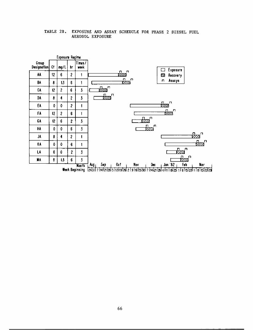
TABLE 2B. EXPOSURE AND ASSAY SCHEDULE FOR PHASE 2 DIESEL FUELAEROSOL EXPOSURE

ixposure Ret ime

GroupDesignation Ct mg/L hr

Times/week

n n• Exposure^ Recoveryn Assays

AA 12 6 2 1 V///A

n n

I Y///ABA 8 1.3 6 1

CA 12 2 6 3n n

l V///A

Aug,

DA 8 4 2 3n n

V//A

EA 0 0 2 1n n

1 V//A

FA 12 2 6 1n n

1 V//A

GA 12 6 2 3n n

1 V//A

HA 0 0 6 3n n

1 V//A

JA 8 4 2 1n n

1 V//A

KA 0 0 6 1n n

1 V//A

LA 0 0 2 3n n

1 V//A

MA 8 1.3 6 3n n

1 V//A

MonthWeek Beginning

Sep | Oct 1 Nov 1 Dec | Jan '82 i Feb | Mar |24l3ll 1Il4l2ll28l 5112ll9l26l 219 Il6l23l3()l 7Il4l2112814 III II8I251118 I5l22lll8lt5l22l29l

66

APPENDIX C: DEFINITIONS AND TABULATED DATA

Exposure:

Frequency:

Concentration:

Time postexposure:

Duration:

Sex:

Ct Product:

The condition of being exposed to diesel fuel aerosol,regardless of concentration, frequency and duration,as opposed to the sham exposures of controls wherediesel fuel aerosol was not Introduced into thechamber.

Either 1 or 3 exposures per week. All animals wereexposed nine times, so that those exposed once perweek were exposed for 9 weeks and those exposed3 times a week were exposed for 3 weeks.

The mass concentration of aerosol in the chamberduring exposure as measured by a mass monitor,calibrated by gravimetric samples (see Table IC).

Half of the animals were assayed in the first two dayspost exposure. The remainder were kept for two weeksafter the last exposure before being assayed in orderto allow either recovery or progression of biologicalchanges due to exposure.

All animals were exposed for either 2 or 6 hours perexposure.

Equal numbers of male and female rats were used ineach exposure group and for determination of eachbiological end point except when this was prevented bymortality.

The multiplication product of concentration (mg/L) andexposure duration (hrs).

67

TABLE IC. MEAN AEROSOL CONCENTRATION DETERMINED GRAVIMETRICALLY

(MEAN ± S.E.) AND TARGET CONCENTRATION FOR EACH TREATMENTGROUP. VALUES ARE IN mg/L.

Hours of ExposureTarget

Concentration

1.33

1.33

2

2

4

4

6

6

Measured

Concentration

ExposureGroup

1.40 ± 0.04 B

1.5 ± 0.05 M

2.18 ± 0.03 F

2.20 ± 0.07 C

4.24 ± 0.03 J

3.88 ± 0.21 D

5.73 ± 0.30 A

5.75 ± 0.09 G

TABLE 2C. LEAST SQUARE MEAN VALUES FOR BODY WEIGHT (g) DIFFERENCESDURING FIRST 2 WEEKS OF EXPOSURE FOR MALES (FEMALES) INRELATION TO EXPOSURE TIME (GRAMS)

Ct Product

mg'hr/L

0

8

12

30.7 (14.4)6.4 (-2.8)

-2.4 (-5.1)

Hours/Exposure

6

27.4 (13.9)-11.1 (-14.3)-8.9 (-9.9) ± 1.7 (1.1)

TABLE 3C. LEAST SQUARE MEAN VALUES FOR BODY WEIGHT (g) DIFFERENCESDURING FIRST 2 WEEKS OF EXPOSURE FOR MALES (FEMALES) INRELATION TO EXPOSURE FREQUENCY

Ct Product

mg'hr/L

0

8

12

27.1 (13.3)14.5 (-0.8)-1.1 (-4.6)

Exposures/Week

68

31.1 (14.9)-19.3 (-16.3)-10.2 (-10.3) ± 1.7 (1.1)

TABLE 4C. LEAST SQUARE MEAN VALUES FOR FOOD CONSUMPTION (g/day) DURINGFIRST 3 WEEKS OF EXPOSURE FOR MALES (FEMALES) IN RELATION TO

Ct PRODUCT

Ct Product

mg'hr/L

Exposure Week

First Second Third

0

8

12

Standard Error

P-Value

29.3 (22.5)27.0 (18.8)25.3 (17.0)0.6 (0.5)0.0002

(0.0001)

29.3 (21.2)26.3 (19.2)26.2 (19.1)0.7 (0.9)

(0.004)(0.19)

29.1 (21.6)26.8 (19.7)26.7 (18.3)

0.7 (0.4)

0.03

(0.0001)

TABLE 5C. LEAST SQUARE MEAN VALUES FOR FOOD CONSUMPTION (g/day) DURINGFIRST 3 WEEKS OF EXPOSURES FOR MALES (FEMALES) IN RELATION TOFREQUENCY OF EXPOSURE

Exposure Week

Exposures/wk First Second Third

1

3

Standard Error

P-value

28.1 (21.0)26.4 (18.9)0.4 (0.4)

0.01

(0.05)

28.6 (20.3)25.9 (19.3)0.5 (0.6)

0.0004

(0.19)

29.2 (20.5)25.8 (19.3)0.5 (0.3)

0.0001

(0.01)

69

TABLE 6C. MILLIONS; of ALVEOLAR MACROPHAGES LAVAGED FROM LUNGS1 DURING

PHASE 2 ASSAYS (MEAN ± S.E.,)

2 Days Postexposure 2 Weeks PostexposureHoursi per

jure

Exnosnrps

mg/L Expos pe r Week Males Females Males Females

0 2 1 2.99±0.54 2.68±0.32 2.67±0.59 2.25±0.480 6 1 1.89±0.23 1.73±0.37 3.95±0.74 2.54±0.370 2 3 2.26±0.52 1.82±0.20 2.48±0.34 1.37±0.190 6 3 2.22±0.20 1.71±0.19 2.48+0.29 1.96±0.414 2 1 4.18±1.03 2.27±0.57 7.28±1.04 4.22±0.594/3 6 1 4.94±0.83 3.14±0.71 6.67±1.01 3.1610.484 2 3 5.83+2.15 5.10±0.73 4.06±0.83 3.5410.474/3 6 3 4.07±0.81 4.33±0.68 4.58±0.63 3.4510.466 2 1 4.74±0.50 3.08±0.68 5.29±0.75 -

2 6 1 6.18±1.17 2.64±0.46 6.18±1.15 3.1310.496 2 3 4.83±0.66 4.48±0.61 3.48±0.46 3.20+0.462 6 3 6.69±0.70 2.99±0.55 9.01±1.91 4.8211.07

TABLE 7C. MILLIONS OF PULMONARY FREE CELLS OTHER THAN ALVEOLAR

MACROPHAGES LAVAGED FROM LUNGS DURING PHASE 2 ASSAYS

(Mean + S.E..)

2 Days Postexposure 2 Weeks PostexposureHours per

ure

Exnisnrps

mg/L Expos per Week Males Females Males Females

0 2 1 2.05±1.20* 1.64±0.90 0.22+0.08 0.1910.040 6 1 0.15±0.04 0.26±0.15 1.40±0.78 0.15+0.030 2 3 0.20±0.04 0.09±0.02 0.24±0.09 0.0910.020 6 3 0.30±0.08 0.12±0.02 0.26±0.12 0.0610.024 2 1 6.99±1.22 4.88±0.58 0.78±0.15 0.4310.104/3 6 1 10.45+2.14 4.26±0.53 0.32±0.07 0.1410.024 2 3 3.75±1.59 2.54±0.63 0.40±0.10 0.25+0.074/3 6 3 3.26±0.55 1.49±0.49 0.11±0.03 0.0910.026 2 1 9.56±2.33 8.21+2.57 0.18±0.06 -

2 6 1 4.92±2.29 3.21±1.24 0.20±0.06 0.1110.066 2 3 3.83±0.72 3.74±0.81 0.61±0.14 0.1710.052 6 3 6.16±2.17 3.85+1.11 0.94±0.27 0.3110.07

*0ne outlier was deleted.

70

TABLE 8C • BINDING INDEX (MEAN NUMBER OF YEAST/MA(:rophage) in

PHAGOCYTOSIS ASSAY OF PHASE 2. (Mean 1 S.E.)

V-v

2 Days Postexposure 2 Weeks Postexposure

riOUta per

mg/L Exposure pe:r Week Males Females Males Females

0 2 1 1.6910.17 1.26+0.10 0.7310.12 0.6610.08

0 6 1 1.1410.12 1.0110.15 1.3810.10 1.4410.25

0 2 3 1.6510.20 1.6010.16 1.5410.13 1.4410.17

0 6 3 1.4710.06 1.3910.14 1.2510.15 1.0010.04

4 2 1 0.9410.11 0.7210.10 1.2210.19 1.0610.17

4/3 6 1 1.1610.07 0.8910.09 0.8610.11 0.8710.08

4 2 3 1.1510.12 1.0310.11 1.0610.26 1.2010.27

4/3 6 3 1.63+0.17 1.4510.19 1.7010.20 2.0610.22

6 2 1 1.1310.18 1.1710.09 1.1310.06 -

2 6 1 1.4210.18 1.3310.11 0.9510.11 0.9710.13

6 2 3 1.0010.12 1.1810.15 1.2610.11 1.20+0.09

2 6 3 0.6310.06 0.6310.10 1.2810.12 1.3510.26

TABLE 9C. PULMONARY RESISTANCE (cm H20/mL/sec) OF RATS IN PHASE 2EXPOSURE TO DIESEL FUEL AEROSOL (Mean 1 S.E.)

Hours per Exposures2 Days Postexposure 2 Weeks Postexposure

mg/L Exposure per Week Males Females Males Females

0 2 1 0.22+0.03 0.4510.10 0.13+0.02 0.1210.03

0 6 1 0.2710.04 0.3610.07 0.2810.03 0.4210.08

0 2 3 0.1110.01 0.2110.08 0.3010.06 0.2310.01

0 6 3 0.5010.06 0.8110.12 0.3710.08 0.4610.09

4 2 1 0.2510.04 0.3210.08 0.2210.04 0.4910.11

4/3 6 1 0.1910.05 0.3610.09 0.1810.03 0.2510.01

4 2 3 0.5110.19 0.5210.14 0.4810.03 0.3710.04

4/3 6 3 0.34+0.03 0.31+0.05 0.17+0.02 0.28+0.02

6 2 1 0.2810.03 0.2210.02 0.2610.02 0.2410.03

2 6 1 0.2010.01 0.53+0.16 0.1210.03 0.1310.01

6 2 3 0.6010.08 0.65+0.11 0.3110.04 0.3710.11

2 6 3 0.3810.11 0.7910.37 0.3010.06 0.4710.10

71

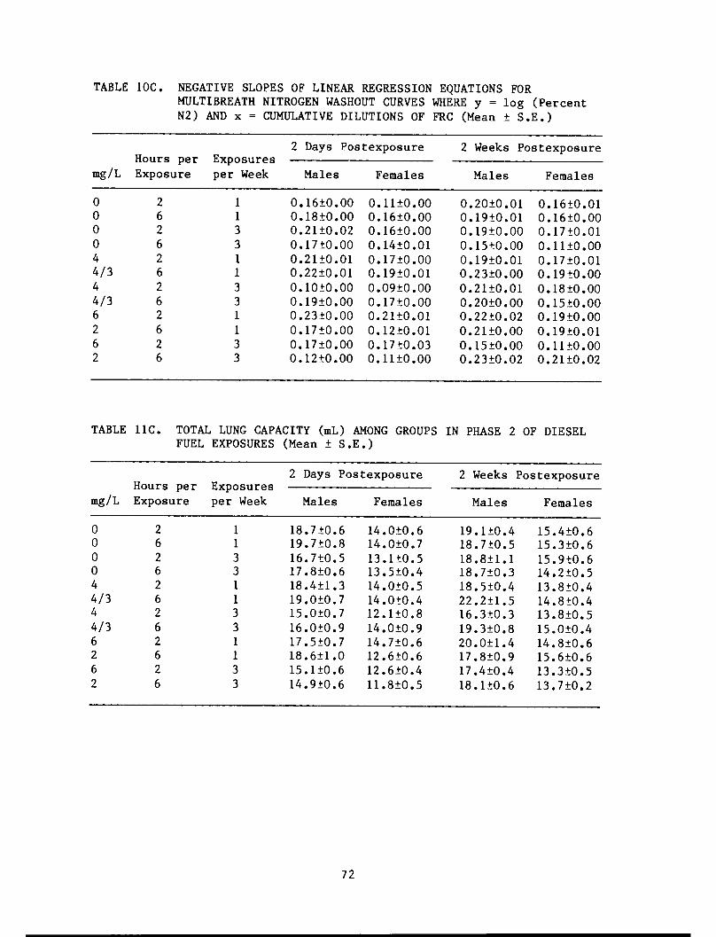
TABLE IOC. NEGATIVE SLOPES OF LINEAR REGRESSION EQUATIONS FORMULTIBREATH NITROGEN WASHOUT CURVES WHERE y = log (PercentN2) AND x = CUMULATIVE DILUTIONS OF FRC (Mean 1 S.E.)

Hours per Exposures

mg/L Exposure per Week

0

0

0

0

4

4/3

4

4/36

2

6

2

2

6

2

6

2

6

2

6

2

6

2

6

1

1

3

3

1

1

3

3

1

1

3

3

2 Days Postexposure

Males

0.1610.00

0.18+0.00

0.2110.02

0.1710.00

0.2110.01

0.2210.01

0.1010.00

0.1910.00

0.2310.00

0.1710.00

0.1710.00

0.12+0.00

Females

0.1110.00

0.1610.00

0.1610.00

0.14+0.01

0.17+0.00

0.1910.01

0.0910.00

0.1710.00

0.21+0.01

0.1210.01

0.1710.03

0.1110.00

2 Weeks Postexposure

Males

0.2010.01

0.1910.01

0.19+0.00

0.1510.00

0.1910.01

0.2310.00

0.2110.01

0.2010.00

0.2210.02

0.2110.00

0.1510.00

0.2310.02

Females

0.1610.01

0.1610.00

0.1710.01

0.1110.00

0.1710.01

0.1910.00

0.1810.00

0.15+0.00

0.1910.00

0.1910.01

0.1110.00

0.21+0.02

TABLE 11C. TOTAL LUNG CAPACITY (mL) AMONG GROUPS IN PHASE 2 OF DIESEL

FUEL EXPOSURES (Mean 1 S.,E.)

2 Days Postexposure 2 Weeks PostexposureHours per

are

Exposi

per Wemg/L Exposi jek Males Females Males Females

0 2 1 18.710.6 14.010.6 19.110.4 15.410.60 6 1 19.710.8 14.010.7 18.710.5 15.310.6

0 2 3 16.710.5 13.110.5 18.811.1 15.910.60 6 3 17.810.6 13.510.4 18.7+0.3 14.210.54 2 1 18.411.3 14.0+0.5 18.510.4 13.810.44/3 6 1 19.0+0.7 14.0+0.4 22.211.5 14.810.44 2 3 15.010.7 12.110.8 16.3+0.3 13.810.54/3 6 3 16.010.9 14.010.9 19.310.8 15.010.46 2 1 17.510.7 14.710.6 20.011.4 14.810.62 6 1 18.611.0 12.610.6 17.810.9 15.610.66 2 3 15.110.6 12.610.4 17.410.4 13.310.52 6 3 14.910.6 11.810.5 18.110.6 13.710.2

72

TABLE 12C. VITAL CAPACITY

EXPOSURES (Mean

(mL) AMONG1 S.E.)

GROUPS IN PH/lSE 2 OF DIEISEL FUEL

Hours Exposures

2 Days Postexposure 2 Weeks Postexposure

per

mg/L Exposure per Week Males Females Males Females

0 2 1 16.410.6 12.410.6 16.410.3 13.310.5

0 6 1 17.110.7 12.210.7 16.210.5 13.410.6

0 2 3 14.410.6 11.310.5 15.710.7 13.610.6

0 6 3 15.7+0.5 11.810.2 16.210.3 12.510.4

4 2 1 15.911.1 12.110.5 15.910.3 11.710.4

4/3 6 1 16.010.7 11.510.3 18.511.4 12.510.4

4 2 3 13.510.6 10.910.6 13.410.3 11.410.4

4/3 6 3 13.210.8 11.810.8 16.110.7 12.710.4

6 2 1 14.310.6 11.910.5 16.511.1 12.310.6

2 6 1 15.210.9 10.310.5 14.910.7 13.210.6

6 2 3 12.510.5 10.210.4 14.810.2 11.310.4

2 6 3 13.310.6 10.010.7 14.610.7 11.210.2

TABLE 13C. INSPIRATORY CAPACITY (mL) AMONG GROUPS IN PHASE 2 OF DIESEL

FUEL EXPOSURES (Mean 1 S.E:.)

Hours Exposures2 Days Postexposure 2 Weeks Postexposure

per

mg/L Exposure per Week Males Females Males Females

0 2 1 15.3+0.5 11.610.4 15.810.3 12.610.6

0 6 1 16.110.7 11.510.7 15.210.5 12.410.5

0 2 3 13.510.5 10.810.4 15.110.8 13.010.4

0 6 3 14.610.4 11.010.2 15.410.4 11.710.4

4 2 1 14.111.1 11.010.4 14.710.4 10.910.3

4/3 6 1 14.710.6 10.5+0.2 16.811.1 11.410.4

1 2 3 12.410.6 10.110.5 12.310.3 10.510.3

4/3 6 3 12.5+0.7 11.0+0.8 15.210.7 12.1+0.4

6 2 1 12.9+0.5 10.810.5 14.9+0.9 11.210.5

2 6 1 14.410.8 9.810.5 14.110.7 12.510.5

6 2 3 11.510.5 9.610.4 13.710.2 10.410.4

2 6 3 12.210.5 9.4+0.4 13.210.6 10.110.2

73

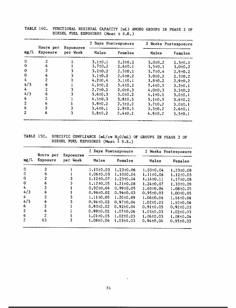
TABLE 14C. FUNCTIONAL RESIDUAL CAPACITY (mL) AMONG GROUPS IN PHASE 2 OFDIESEL FUEL EXPOSURES (Mean 1 S.E.)

mg/L

0

0

0

0

4

4/34

4/36

2

6

2

Hours per

Exposure

2

6

2

6

2

6

2

6

2

6

2

6

Exposures

per Week

1

1

3

3

1

1

3

3

1

1

3

3

2 Days Postexposure

Males

3.110.1

3.710.2

3.210.2

3.110.2

4.210.4

4.310.2

2.710.2

3.610.3

4.510.3

3.910.2

3.410.1

2.810.2

Females

2.210.2

2.610.1

2.310.1

2.410.2

3.110.1

3.410.2

2.010.3

3.010.2

3.810.3

2.510.2

2.9+0.5

2.410.2

2 Weeks Postexposure

Males

3.010.2

3.510.1

3.710.4

3.0+0.2

3.810.2

5.410.5

4.010.3

4.110.1

5.110.5

3.7+0.2

3.310.2

4.910.2

Females

2.510.1

3.010.2

2.910.2

2.310.2

2.910.2

3.310.1

3.310.2

3.010.1

3.610.2

3.010.1

2.610.1

3.510.1

TABLE 15C. SPECIFIC COMPLIANCE (mL/cm H20/mL) OF GROUPS IN PHASE 2 OFDIESEL FUEL EXPOSURES (Mean 1 S.E.)

2 Days Postexposure 2 Weeks PostexposureHours per

Exposure

Exposures

per Weekmg/L Males Females Males Females

0 2 1 1.1010.03 1.2310.06 1.2010.04 1.23+0.080 6 1 1.0610.03 1.1010.04 1.1110.06 1.1210.050 2 3 1.1210.07 1.2310.04 1.1410.11 1.1710.080 6 3 1.1210.05 1.2110.08 1.2410.07 1.3310.094 2 1 0.9210.04 0.9910.05 1.03+0.04 1.0810.054/3 6 1 0.9610.02 0.9410.03 0.9510.03 1.0010.054 2 3 1.1110.05 1.2010.09 1.06+0.06 1.1610.064/3 6 3 0.9410.02 0.9710.04 1.0210.03 1.1010.066 2 1 0.9310.02 0.9210.04 0.9110.05 0.92+0.032 6 1 0.9910.02 1.0710.06 1.0310.03 1.0210.036 2 3 1.0110.05 1.0210.03 1.0610.03 1.0810.042 63 3 1.0810.06 1.03+0.03 0.9410.04 0.95+0.03

74

TABLE 16C. PEAK FLOW (mL/sec) III tlAXIMikh FOBtci!D EXI'IRATIC)N MANE:UVER /WONG

GROUPS IN PHASE 2 OF DIESEL FUEL EXPOSURES (MEAN 1 S.E.)

Hours Expos

2 Days Postexposure 2 Weeks Postexposure

per ures

mg/L Exposure per Week MalesI Females Males Females

0 2 1 47.4 + 1.6 35.6 + 1.5 47.5 1 0.9 42.0 1 2.3

0 6 1 51.2 + 2.0 39.3 + 1.9 49.1 1 1.5 40.4 1 1.1

0 2 3 45.2 + 1.8 36.4 + 2.0 47.4 1 1.4 41.2 1 1.1

0 6 3 38.4 + 1.8 31.1 + 1.3 47.4 1 1.3 37.5 + 1.5

4 2 1 44.7 + 2.2 33.4 + 2.6 46.3 1 1.2 34.7 + 2.5

4/3 6 1 48.9 + 1.5 38.5 + 0.6 52.3 1 2.7 40.5 1 1.2

4 2 3 37.2 + 2.0 32.9 + 2.0 42.9 + 1.3 37.1 1 1.0

4/3 6 3 39.4 + 1.9 37.6 + 2.2 46.7 1 1.7 37.4 1 1.4

6 2 1 44.2 + 1.0 34.2 + 1.6 49.9 1 1.9 38.6 1 2.6

2 6 1 44.5 + 1.5 29.7 + 1.7 42.3 1 2.2 39.4 1 2.8

6 2 3 29.5 + 2.4 26.3 + 1.4 42.8 1 0.7 35.3 1 0.9

2 6 3 35.0 + 2.3 28.1 + 2.0 42.6 1 2.3 37.4 1 0.5

TABLE 17C • EXPIRATORY FLOW (mL/sec) AT 50 PE:rc:ent oiF VITAlL CAPAiCITY r(URING

MAXIMAL FORCED EXPIRATION MANEUVER AMONG GROUPS IN PHASE 2I OF

DIESEL FUEL EXPOSURES! (MEAN 1 S.E:.)I

2 Days Postexposure 2 Weeks Postexposure

Hours per bxpuaures

mg/L Exposure

2

per Week Males Females Males Females

0 1 43.4 1 2.0 30.2 + 1.6 42.8 1 0.9 36.5 1 2.6

0 6 1 46.8 1 2.7 34.0 + 2.2 45.8 1 1.6 36.7 1 1.1

0 2 3 40.7 1 2.2 31.7 + 1.9 43.7 1 1.5 36.7 1 1.1

0 6 3 34.8 1 2.4 25.9 + 1.5 44.1 1 1.6 32.1 1 1.9

4 2 1 39.7 1 2.3 29.8 + 2.0 43.9 1 9.9 30.5 1 2.2

4/3 6 1 44.5 1 1.9 33.2 + 0.9 48.7 1 3.5 35.2 1 1.3

4 2 3 33.1 + 2.5 28.9 + 2.1 38.6 1 1.3 32.0 1 1.2

4/3 6 3 34.8 1 1.9 33.8 + 2.0 42.7 1 1.4 32.7 1 1.3

6 2 1 40.4 1 1.2 31.0 + 1.5 45.2 1 2.4 33.4 1 2.9

2 6 1 39.9 + 1.8 25.1 + 1.8 37.5 1 2.3 34.5 1 2.5

6 2 3 24.8 1 2.1 21.6 + 1.5 38.5 1 0.8 30.0 1 1.1

2 6 3 33.3 1 2.6 25.3 + 1.9 39.9 1 2.7 32.6 1 0.7

75

TABLE 18C. EXPIRATORY FLOWf (mL/isec) AFTER EXHALATION OF 75 PERCENT OF VITAL

CAPACITY DURING: MAXIMAL FORCED EXPIRATION MANEUVER AMONG GROUPSIN PHASE 2 OF DIESEL FUEL EXPOSURES1 (MEAN 1 S.E .)

2 !Days Postexposure 2 Weeks PostexposureHours per

ure

Exposi

per We

ires

mg/L Expos' ;ek Males Females Males Females

0 2 1 25.8 1 1.3 16.9 1 0.9 23.8 1 1.3 20.4 1 1.30 6 1 26.4 1 1.4 20.2 1 1.1 26.1 1 0.9 21.9 1 0.70 2 3 22.8 1 1.4 18.4 1 1.2 25.2 1 1.1 21.3 1 0.70 6 3 19.1 1 1.9 13.9 + 1.0 26.3 1 0.8 18.1 1 1.44 2 1 22.8 1 1.0 17.6 1 1.1 25.6 1 0.4 27.6 1 1.24/3 6 1 25.9 1 1.2 19.0 1 0.9 28.3 1 2.0 20.6 1 0.84 2 3 19.8 1 2.0 16.6 1 1.1 22.2 1 0.7 18.3 1 1.04/3 6 3 19.9 1 1.1 19.7 1 1.1 24.1 1 0.8 19.2 + 0.66 2 1 23.1 1 0.7 19.3 1 0.7 25.7 1 1.3 19.7 1 1.92 6 1 21.7 1 1.1 14.0 1 1.1 21.3 1 1.3 20.0 1 1.86 2 3 13.9 1 0.9 11.4 1 0.9 21.6 1 0.8 17.1 1 0.82 6 3 20.4 1 2.5 17.0 1 1.4 23.1 1 1.4 18.6 1 0.6

TABLE 19C. EXPIRATORY FLOW (mL/sec) AT 50 PERCENT OF VITAL CAPACITY DURING

MAXIMAL FORCED EXPIRATION MANEUVER REFERENCED TO VITAL CAPACITY(mL) . VALUES ARE MEAN 1 S.Ei •

2 Days Postexposure 2 Weeks PostexposureHours per

ire

Exposu

per We

ires

mg/L Expost ek Males Females Males Females

0 2 1 2.65 1 0.05 2.45 1 0.09 2.62 1 0.08 2.74 1 0.120 6 1 2.74 1 0.11 2.80 1 0.08 2.83 1 0.06 2.75 1 0.070 2 3 2.82 1 0.07 2.79 1 0.07 2.80 1 0.08 2.71 1 0.100 6 3 2.22 1 0.14 2.19 1 0.09 2.73 1 0.08 2.58 1 0.174 2 1 2.52 1 0.10 2.48 1 0.15 2.71 1 0.05 2.58 1 0.124/3 6 1 2.78 1 0.06 2.89 1 0.03 2.63 1 0.08 2.81 1 0.074 2 3 2.47 1 0.13 2.64 1 0.11 2.88 + 0.10 2.80 1 0.084/3 6 3 2.65 1 0.08 2.87 + 0.04 2.66 1 0.05 2.57 1 0.056 2 1 2.84 1 0.09 2.62 1 0.14 2.77 1 0.10 2.71 1 0.162 6 1 2.63 1 0.07 2.43 + 0.11 2.52 1 0.08 2.60 1 0.136 2 3 1.99 1 0.16 2.12 1 0.13 2.61 1 0.07 2.66 1 0.082 6 3 2.51 1 0.16 2.46 1 0.14 2.72 1 0.07 2.91 1 0.06

76

TABLE 20C. SINGLE-BREATH CARBON MONOXIDE DIFFUSING CAPACITY (mL/(mmHg) (min))AMONG GROUPS IN PHASE 2 OF DIESEL FUEL EXPOSURES (MEAN 1 S.E.)

2 Days Postexposure 2 Weeks PostexposureHours per

ure

Exposures

per Weekmg/L Exposi Males Females Males Females

0 2 1 1.16 + 0.07 0.61 1 0.04 1.22 1 0.04 0.75 + 0.090 6 1 1.18 + 0.07 0.74 1 0.08 1.15 1 0.07 0.79 + 0.060 2 3 1.13 + 0.06 0.67 1 0.08 1.34 1 0.09 0.88 + 0.060 6 3 1.18 + 0.05 0.73 1 0.03 1.28 1 0.07 0.81 + 0.04

4 2 1 1.07 + 0.07 0.69 1 0.04 1.18 + 0.03 0.68 + 0.04

4/3 6 1 1.47 + 0.15 0.77 1 0.04 1.25 1 0.11 0.62 + 0.06

4 2 3 0.73 + 0.03 0.40 1 0.03 1.12 1 0.05 0.67 + 0.03

4/3 6 3 1.07 + 0.09 0.72 1 0.08 1.20 + 0.11 0.70 + 0.04

6 2 1 1.06 + 0.07 0.66 1 0.03 1.26 1 0.08 0.63 + 0.04

2 6 1 1.06 + 0.13 0.59 1 0.03 1.02 1 0.10 0.65 + 0.03

6 2 3 0.76 + 0.03 0.50 1 0.05 1.10 1 0.04 0.57 + 0.08

2 6 3 0.97 + 0.07 0.45 1 0.02 0.64 1 0.06 0.25 + 0.03

TABLE 21C. SINGLE BREATH (:arbon MONOXIDE DIFFUSING CAPACITY REFERENCED TO

TOTAL LUNG CAPACITY 1[IN LITERS) AMONG GROUPS IN PHASE 2 OF DIESELFUEL EXPOSURES (MEAN + S.E.)

2 Days Postexposure 2 Weeks PostexposureHnilTQ T\£i t" Exposures

per Weekmg/LL1UUL 3 ls<w.j.

Exposure Male!S Females Males Females

0 2 1 71.5 + 4.8 49.4 1 2.2 74.6 1 1.9 56.1 + 5.,3

0 6 1 69.5 + 4.7 61.3 1 6.4 71.1 1 3.7 59.6 1 5..3

0 2 3 78.7 + 4.1 58.2 1 5.0 85.5 1 4.5 64.5 1 3.,0

0 6 3 75.8 + 3.2 62.0 1 2.9 79.0 1 3.2 65.1 1 4.,3

4 2 1 69.0 + 6.6 57.8 1 3.1 74.2 1 1.4 57.3 1 4.,14/3 6 1 93.1 + 10.9 67.3 1 3.5 67.4 1 3.9 49.6 + 4.,0

4 2 3 54.2 + 1.8 36.9 1 2.9 84.0 1 4.4 58.4 1 1.,9

4/3 6 3 81.1 + 6.0 60.7 1 4.1 73.5 + 4.5 55.6 1 4.,4

6 2 1 73.5 + 2.1 55.6 1 2.5 76.5 1 1.6 51.1 1 3.,1

2 6 1 68.4 + 6.7 57.6 1 2.7 67.9 1 5.5 49.7 1 2. 5

6 2 3 60.9 + 2.8 48.6 1 2.9 74.8 1 2.3 50.0 1 6.,8

2 6 3 73.1 + 5.1 47.1 1 5.1 44.7 1 5.2 22.2 1 2.,0

77

TABLE 22C. LIVER WEIGHT (g) AMONG GROUPS IN PHASE 2 OF DIESEL FUELEXPOSURES (MEAN 1 S.E.)

2 Days Postexposure 2 Weeks PostexposureHours per exposures

mg/L Exposure

2

per Week Males Females Males Females

0 1 15.610.9 9.3+0.3 18.110.7 11.1+0.8

0 6 1 15.510.5 10.210.8 18.110.9 9.8+0.2

0 2 3 14.810.5 9.110.4 15.410.9 9.710.5

0 6 3 14.310.3 10.010.5 14.310.8 9.610.5

4 2 1 14.810.6 8.710.3 15.710.2 8.310.3

4/3 6 1 14.6+0.6 8.910.2 14.8+0.7 8.2+0.4

4 2 3 14.4+0.2 8.410.3 14.710.9 8.410.2

4/3 6 3 14.410.4 8.810.3 15.8+0.8 9.610.3

6 2 1 14.610.7 8.3+0.3 17.110.6 8.410.5

2 6 1 15.7+0.9 8.010.5 15.710.6 8.9+0.3

2 2 3 14.110.9 8.310.3 14.410.6 9.1+0.2

6 6 3 14.210.7 8.210.2 15.2+0.8 8.610.3

TABLE 23C. KIDNEY WEIGHT (jt) AMONG GRi0UPS IN PHASIE 2 OF DIES!EL FUEL

EXPOSURES (MEAN 1 S.E.)

Hours Expos

2 Days Postexposure 2 Weeks Postexposure

per ures

mg/L Exposure per Week Males Females Males Females

0 2 1 1.6610.05 0.9810.03 1.83+0.08 1.1310.04

0 6 1 1.65+0.04 1.0410.07 1.7810.09 1.1210.04

0 2 3 1.44+0.03 0.93+0.14 1.5710.11 0.9810.04

0 6 3 1.4710.05 0.96+0.04 1.5410.02 1.0410.05

4 2 1 1.6210.06 0.8510.02 1.70+0.06 0.9410.04

4/3 6 1 1.5910.08 0.95+0.04 1.7110.09 0.9510.02

4 2 3 1.4810.03 0.9110.01 1.6110.07 0.9910.04

4/3 6 3 1.4910.07 0.9310.04 1.6510.04 0.97+0.04

6 2 1 1.52+0.07 0.8410.03 1.81+0.08 0.8610.06

2 6 1 1.67+0.09 0.8910.04 1.6010.06 1.00+0.06

6 2 3 1.4710.07 0.8510.05 1.6010.08 1.0010.03

2 6 3 1.54+0.06 0.8710.02 1.58+0.10 1.01+0.04

TABLE 24C. WEIGHT OF ADRENAL GLANDS (mg) AMONG GROUPS :IN PHASE 2 OF

DIESEL FUEL EXPOSURES (MEAN 1 S,.E •)

2 Days Postexposure 2 Weeks Post:exposure

mg/L Exposure pesr Week Males Females Males Females

0 2 1 26 1 1 36 + 2 27 1 1 34 1 20 6 1 24 1 2 30 + 2 26 1 2 34 1 3

0 2 3 29 1 1 33 + 1 28 1 3 35 1 2

0 6 3 28 1 2 35 + 2 33 1 2 34 1 2

4 2 1 26 1 3 32 + 1 25 1 3 29 1 2

4/3 6 1 28 1 1 33 + 3 29 1 2 33 1 2

4 2 3 29 1 2 32 + 2 25 1 2 37 1 2

4/3 6 3 28 1 1 32 + 1 28 1 2 29 1 4

6 2 1 26 1 2 32 + 3 29 1 2 32 1 4

2 6 1 30 1 2 30 + 3 26 1 1 34 1 2

6 2 3 27 1 1 36 + 1 32 1 1 42 1 1

2 6 3 30 1 1 31 + 2 32 1 2 37 1 1

TABLE 25C. WET WEIGHT OF RIGHT MIDDLE LUNG LOBE (mg) AMONG GROUPS IN

PHASE 2 OF DIESEL FUEL EXPOSURES (MEAN i S.E.)

2 Days Postexposure 2 Weeks Postexposureper

are

Exposi

per Wemg/L Exposi ;ek Males Females Males Females

0 2 1 189 1 9 134 1 8 179 1 7 141 i 7

0 6 1 170 116 133 1 8 170 ilO 143 1 3

0 2 3 159 1 6 120 1 4 160 1 8 121 i 4

0 6 3 177 112 136 1 9 180 1 7 150 1 6

4 2 1 216 110 156 1 5 202 + 8 141 1 6

4/3 6 1 214 ill 149 1 5 211 112 148 1 3

4 2 3 213 1 8 157 1 6 190 1 7 145 1 8

4/3 6 3 219 1 9 154 1 5 176 i 6 145 i 5

6 2 1 236 113 180 1 9 227 + 6 163 +15

2 6 1 257 113 161 1 5 198 115 145 ± 62 2 3 248 1 9 196 ill 220 + 12 174 1 4

6 6 3 246 113 196 i 9 196 1 4 145 + 7

79

TABLE 26C. WET/DRY WEIGHT RATIOS OF RIGHT MIDDLE LUNG LOBES AMONGGROUPS IN PHASE 2 OF DIESEL FUEL EXPOSURES (MEAN 1 S.E.)

2 Days Postexposure 2 Weeks PostexposureHours per Exposures

mg/L Exposure per Week

0 2

0 6

0 2

0 6

4 2

4/3 6

4 2

4/3 6

6 2

2 6

2 2

6 6

1

1

3

3

1

1

3

3

1

1

3

3

Males

5.0410.03

5.20+0.04

5.3310.03

5.0410.03

5.0110.04

5.1010.03

5.1710.05

5.1910.04

4.7310.17

5.1410.05

5.2410.06

5.1110.04

Females

5.0410.05

5.1110.05

5.3810.04

5.09+0.05

5.1810.05

5.0110.04

5.1010.05

5.3210.05

4.8910.17

5.2210.05

5.2010.02

5.2110.04

Males

5.1210.03

5.1910.06

5.1710.06

5.3510.06

5.1710.01

5.21+0.05

5.0410.05

5.1910.02

4.9610.05

5.0910.03

5.0810.04

5.11+0.03

Females

5.0110.03

5.2310.05

5.2010.05

5.2610.07

5.2010.05

5.1810.05

5.0710.08

5.04+0.06

4.9210.04

5.1710.06

4.9210.12

5.0310.09

TABLE 27C. SEVERITY OF FOCAL PNEUMONITIS AND ASSOCIATED HISTOLOGICALCHANGES AMONG GROUPS IN PHASE 2 OF DIESEL FUEL EXPOSURES

mg/LHours perExposure

Exposuresper Week 2 Days Postexposure 2 weeks Postexposure

0 2

0 6

0 2

0 6

4 2

4/3 6

4 2

4/3 6

6 2

2 6

2 2

6 6

1

1

3

3

1

1

3

3

1

1

3

3

+

+/-H"++/-H-f+

•H-/-H-+

-, no observed focal pneumonitis,i, equivocal change,

+, slight,•+, moderate,

most severe observed.

80

+

±7+++

±/++

+

+/-H

TABLE 28C. PRE-EXPOSURE FORELIMB GRIP STRENGTH (kg) AMONG GROUPS INPHASE 2 OF DIESEL FUEL EXPOSURES (Mean 1 S.E.)

Hours per Exposuresmg/L Exposure per Week Males Females

0 2 1 0.91 1 0.04 0.78 1 0.05

0 6 1 1.02 i 0.04 0.74 1 0.04

0 2 3 0.98 1 0.02 0.76 1 0.04

0 6 3 0.78 i 0.07 0.85 1 0.04

4 2 1 0.94 1 0.06 0.77 1 0.04

4/3 6 1 1.09 1 0.06 0.92 1 0.03

4 2 3 1.00 i 0.09 0.88 1 0.06

4/3 6 3 0.82 1 0.07 0.90 1 0.03

6 2 1 1.03 i 0.05 0.93 i 0.03

2 6 1 0.97 1 0.08 0.71 1 0.07

6 2 3 1.03 1 0.04 0.81 i 0.06

2 6 3 1.07 1 0.04 0.96 i 0.04

TABLE 29C. PRE-EXPOSURE LANDING FOOT SPREAD (mm) AMONG GROUPS IN

PHASE! 2 OF DIESEL FUEL EXPOSURES (MEAN 1 S.E:.)

Hours per Exposuresmg/L Exposure per Week Male>S Females

0 2 1 110 1 10 98 1 1

0 6 1 108 1 8 80 1 5

0 2 3 102 i 8 96 i 6

0 6 3 113 1 8 102 110

4 2 1 106 i 5 81 1 4

4/3 6 1 134 1 13 88 1 4

4 2 3 132 1 4 88 i 4

4/3 6 3 127 1 5 94 1 8

6 2 1 112 1 9 95 1 6

2 6 1 110 ± 8 97 +11

6 2 3 107 1 1 95 ill

2 6 3 111 1 8 95 i 8

81

TABLE 30C. PRE-EXPOSURE TAIL FLICK REFLEX (sec) AMONG GROUPS IN 1PHASE 2

OF DIESEL FUEL EXPOSURES (Mean 1 S,.S,.)

Hours per Exposuresmg/L Exposure per Week Males Females

0 2 1 1.82 + 0.17 1.45 + 0.08

0 6 1 1.54 + 0.16 1.09 + 0.08

0 2 3 1.35 + 0.13 1.27 + 0.17

0 6 3 1.80 + 0.15 1.63 + 0.10

4 2 1 1.50 + 0.25 1.35 + 0.14

4/3 6 1 1.76 + 0.13 1.71 + 0.15

4 2 3 2.09 + 0.31 1.59 + 0.09

4/3 6 3 2.14 + 0.29 1.87 + 0.12

6 2 1 1.76 + 0.11 1.54 + 0.12

2 6 1 1.82 + 0.09 1.78 + 1.0

6 2 3 1.56 + 0.17 1.49 + 0.04

2 6 3 1.62 + 0.18 1.51 + 0.10

TABLE 31C. PRE-EXPOSURE PEAK HEIGHT (g;ram weight) IN STARTLE REFLEX

AMONG GROUPS IN PHASE 2 OF DIESEL FUEL EXPOSURES

(MEAN i s.e.:)

Hours per Exposuresmg/L Exposure per Week Males Females

0 2 1 359 1 64 166 i 25

0 6 1 433 1 39 330 1 80

0 2 3 432 1 72 388 1 59

0 6 3 298 1 51 252 1 47

4 2 1 227 + 43 135 + 20

4/3 6 1 382 ± 70 135 ± 35

4 2 3 313 1 49 261 + 53

4/3 6 3 463 i 81 346 1 46

6 2 1 339 + 35 212 1 19

2 6 1 286 i 34 172 1 32

6 2 3 272 1 35 229 1 35

2 6 3 475 1 48 215 1 49

82

TABLE 32C. PRE-EXPOSURE PEAK TIME (msec) IN STARTLE REFLEX ASSAY AMONGGROUPS IN PHASE 2 OF DIESEL FUEL EXPOSURES (MEAN i S.E.)

mg/LHours perExposure

0 2

0 6

0 2

0 6

4 2

4/3 6

4 2

4/3 6

6 2

2 6

6 2

2 6

Exposuresper Week Males Females

1 26.8 + 0.5 26.1 i 0.3

1 26.8 + 0.4 27.2 1 2.1

3 27.6 + 0.8 25.3 1 0.3

3 27.1 + 0.9 27.5 1 1.2

1 27.6 + 0.9 24.7 1 0.4

1 27.2 + 0.7 25.6 1 0.5

3 26.4 + 0.4 27.4 i 1.5

3 26.5 + 0.7 27.4 1 0.8

1 27.1 + 1.0 26.3 1 0.6

1 26.1 + 0.5 29.1 1 2.7

3 27.3 + 1.0 26.4 1 0.9

3 31.2 + 2.1 25.7 i 0.7

TABLE 33C. PRE-EXPOSURE REACTION TIME (msec) IN STARTLE REFLEX ASSAYAMONG GROUPS IN PHASE 2 OF DIESEL FUEL EXPOSURES

(MEAN 1 S.E.)

mg/LHours perExposure

0 2

0 6

0 2

0 6

4 2

4/3 6

4 2

4/3 6

6 2

2 6

6 2

2 6

Exposuresper Week Males Females

1 18.0 + 0.4 18.0 1 0.3

1 17.4 + 0.3 18.8 1 2.0

3 18.3 + 0.5 17.3 1 0.5

3 18.3 + 0.3 16.9 1 0.6

1 18.3 + 0.4 16.7 1 0.3

1 18.2 + 0.5 19.0 i 0.5

3 17.1 + 0.4 18.0 1 1.2

3 16.9 + 0.4 16.9 i 0.3

1 17.8 + 0.4 17.4 + 0.3

1 17.4 + 0.6 18.6 1 3.5

3 18.1 + 0.2 17.7 i 0.6

3 19.6 + 0.9 16.6 1 1.0

83

TABLE 34C. LEAST SQUARES MEANS OF CLINICAL CHEMISTRY PARAMETERS

IN SHAM-EXPOSED GROUPS (1 S.E.)

Alkaline phosphatase (mU/mL)SGOT (mU/mL)Cholesterol (mg percent)Triglycerides (mg percent)Uric acid (mg percent)Glucose (mg percent)Urea nitrogen (mg percent)Total bilirubin (mg percent)Creatinine (mg percent)Sodium (mEq percent)Potassium (mEq percent)

84

Males Females

150 + 7 108 1 7

155 1 5 134 1 5

54.8 1 2.3 70.7 1 2.3

119 1 7 128 1 7

2.15 + 0.08 1.74 + 0.07

174 1 5 153 1 5

23.4 1 0.5 24.0 1 0.5

0.59 1 0.04 0.65 1 0.04

0.79 1 0.04 0.82 1 0.03

145 1 0.4 145 1 0.4

4.86 1 0.12 3.96 1 0.11

APPENDIX D:

HISTOPATHOLOGY

The following pages contain notes on histopathological evaluation ofIndividual animals at 2 days after the last exposure. All slides werecoded by number so that the pathologist could not identify groups. Theterm "SD pneumonitis" is used for the pulmonary lesions observed inunexposed Sprague-Dawley rats, consisting primarily of peribronchial andperivascular inflammation with some focally Increased numbers of pulmonaryfree cells In the alveoli. The term "alveolitis" refers to chronicinfiltrate on the walls of the alveoli but not the lumen. The notation of"macrophages" refers to alveolar macrophages and other free cells withinthe alevoli. Animals are coded by a number and M for males or F forfemales. Individual data are not presented for animals examined at twoweeks post exposure. There were no exposure-related changes observed intissues other than the lung among these animals. The primary question,therefore was whether pulmonary lesions observed at 2 days postexposurewere altered by the two week interim without exposure. This question wasanswered by blind scoring of the lesions on the basis of groups rather thanindividuals, as shown in Table 27C.

The following scoring criteria were used in the histopathologicalevaluations:

1, equivocal change,+, slight,

++, moderate,+++, most severe observed.

85

GROUP EA (0 mg/L, 2 hr/exposure, 1 exposure/wk)2 days Postexposure

Animal

13 M

14 M

15 M

16 M

17 M

18 M

13 F

14 F

15 F

16 F

17 F

18 F

Some SD pneumonitisSome SD pneumonitis, macrophages (+)normal

Some SD pneumonitis, macrophages (+)Some SD pneumonitisSD pneumonitis, alveolitis, macrophages (+), sinusitisSome SD pneumonitis

normal

Some SD pneumonitisSome SD pneumonitis, macrophages (+)normal

normal

GROUP LA (0 mg/L, 2 hr/exposure, 3 exposures/wk)2 Days Postexposure

Animal

13 M

14 M

15 M

16 M

17 M

18 M

13 F

14 F

15 F

16 F

17 F

18 F

few macrophagesfew macrophagesfew macrophages

few macrophagessame with sinusitis

more cellularlty and macrophages, slight squamousmetaplasia In larynx

few macrophagesfew macrophagesfew macrophagesmore cellularlty and macrophages, slight squamous

metaplasia in larynx

few macrophagesfew macrophages

86

GROUP KA (0 mg/L, 6 hr/exposure, 1 exposure/wk)2 Days Postexposure

Animal

13 M almost normal, some SD pneumonitis fociAll other animals were the same with some atrophic epitheliumin the trachea.

GROUP HA (0 mg/L, 6 hr/exposure, 3 exposures/wk)2 Days Postexposure

Animal

normal

glomerular hypercellularityglomerular changes, chronic sinusitis and rhinitis

(infiltration and squamous metaplasia)16 M renal tubular cloudy swelling, lung congestion, some

alveolar macrophages17 M SD infiltrate in lung (++), renal tubular swelling18 M liver congestion, very slight centrilobular swelling,

lymphocytic infiltrate, hepatocellular swelling13 F glomerular changes, slight hepatic infiltrate, slight

alveolar rupture, sinusitis and slight rhinitis14 F SD infiltrate in lung (+)15 F centrilobular congestion and disintegration in liver

(cloudy swelling and necrosis), sinusitis andrhinitis

16 F Some alveolar macrophages, ruptured alveoli, livercongestion and hepatocellular swelling, slightinterstitial medullary nephritis, slight laryngitis

17 F normal

18 F slight laryngitis

13 M

14 M

15 M

87

GROUP JA (4 mg/L, 2 hr/exposure, 1 exposure/wk)2 Days Postexposure

Animal

13 M lung almost normal, some focal14 M lung almost normal, some focal

15 M lung almost normal, some focal16 M lung almost normal, some focal

17 M lung almost normal, some focal

18 M lung almost normal, some focal13 F lung almost normal,

macrophagessome facal

14 F lung almost normal, some focal15 F lung almost normal, some focal16 F lung almost normal, some focal17 F lung almost normal, some focal18 F lung almost normal, some focal

pneumonitis

pneumonitis, rhinitis

pneumonitispneumonitis

pneumonitis

pneumonitis

pneumonitis with more

pneumonitis

pneumonitis

pneumonitis

pneumonitis

pneumonitis

GROUP DA (4 mg/L, 2 hr/exposure, 3 exposures/wk)2 Days Postexposure

Animal

13 M

14 M

15 M

16 M

17 M

18 M

13 F

14 F

15 F

16 F

17 F

18 F

macrophages (++), ruptured wallsmacrophages (+), SD pneumonitis, sinusitislung congestion, few macrophagesnormal

normal

normal, sinusitisnormal

almost normal, SD pneumonitis, sinusitisalmost normal, SD pneumonitis, sinusitisnormal

normal, sinusitisnormal, sinusitis

88

GROUP BA (1-1/3 mg/L, 6 hr/exposure, 1 exposure/wk)2 Days Postexposure

Animal

13 M Some hypercellular alveolar walls, ruptured walls, fewmacrophages

14 M Some hypercellular alveolar walls, ruptured walls, fewmacrophages, SD pneumonitis

15 M Some hypercellular alveolar walls, ruptured walls, fewmacrophages

16 M Some hypercellular alveolar walls, ruptured walls, fewmacrophages, focus acute colonjitis

17 M Some hypercellular alveolar walls, ruptured walls, fewmacrophages

18 M Some hypercellular alveolar walls, ruptured walls, fewmacrophages, SD pneumonitis

13 F Some hypercellular alveolar walls, ruptured walls, fewmacrophages but less severe

14 F Some hypercellular alveolar walls, ruptured walls, fewmacrophages but less severe

15 F Some hypercellular alveolar walls, ruptured walls, fewmacrophages, SD pneumonitis

16 F SD pneumonitis, almost normal17 F Some hypercellular alveolar walls, ruptured walls, few

macrophages, focus of Interstitial nephritis18 F SD pneumonitis, almost normal

GROUP MA (1 1/3 mg/L, 6 hr/exposure, 3 exposures/wk)2 Days Postexposure

Animal

13 M

14 M

15 M

16 M

17 M

18 M

13 F

14 F

15 F

16 F

17 F

18 F

alveolar cellularlty, few macrophages, sinusitisalveolar cellularlty, atrophic tracheal epitheliumalveolar cellularlty, atrophic tracheal epitheliumalveolar cellularlty, macrophages, atrophic tracheal

epitheliumalveolar cellularlty, macrophages, atrophic tracheal

epitheliumalveolar cellularlty, macrophages, atrophic tracheal

epitheliumalmost normal

alveolar cellularlty, macrophages, atrophic trachealepithelium

alveolar cellularlty, macrophages, atrophic trachealepithelium

alveolar cellularlty, macrophages, atrophic trachealepithelium

almost normal

alveolar cellularlty, macrophages, atrophic trachealepithelium

89

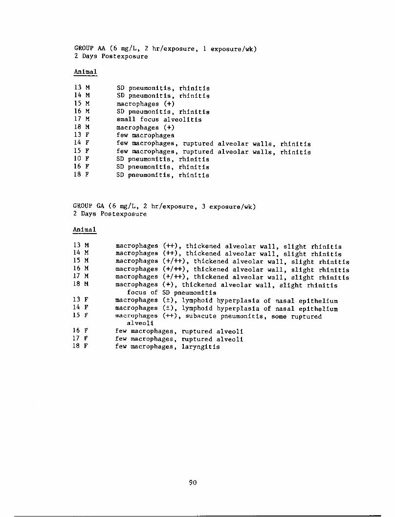
GROUP AA (6 mg/L, 2 hr/exposure, 1 exposure/wk)2 Days Postexposure

Animal

13 M

14 M

15 M

16 M

17 M

18 M

13 F

14 F

15 F

10 F

16 F

18 F

SD pneumonitis, rhinitisSD pneumonitis, rhinitis

macrophages (+)SD pneumonitis, rhinitissmall focus alveolitis

macrophages (+)few macrophagesfew macrophages, ruptured alveolar walls, rhinitisfew macrophages, ruptured alveolar walls, rhinitisSD pneumonitis, rhinitisSD pneumonitis, rhinitis

SD pneumonitis, rhinitis

GROUP GA (6 mg/L, 2 hr/exposure, 3 exposure/wk)2 Days Postexposure

Animal

13 M

14 M

15 M

16 M

17 M

18 M

13 F

14 F

15 F

16 F

17 F

18 F

macrophages (++), thickened alveolar wall, slight rhinitismacrophages (++) , thickened alveolar wall, slight rhinitismacrophages (+/++), thickened alveolar wall, slight rhinitismacrophages (+/++), thickened alveolar wall, slight rhinitismacrophages (+/++), thickened alveolar wall, slight rhinitismacrophages (+), thickened alveolar wall, slight rhinitis

focus of SD pneumonitismacrophages (i), lymphoid hyperplasia of nasal epitheliummacrophages (1), lymphoid hyperplasia of nasal epitheliummacrophages (++), subacute pneumonitis, some ruptured

alveoli

few macrophages, ruptured alveolifew macrophages, ruptured alveolifew macrophages, laryngitis

90

GROUP FA (2 mg/L, 6 hr/exposure, 1 exposure/wk)2 Days Postexposure

Animal

13 M

14 M

15 M

16 M

17 M

18 M

13 F

14 F

15 F

16 F

17 F

18 F

macrophages (+),rupture, foci

macrophages (+),rupture, foci

macrophages (+),rupture, foci

macrophages (++)macrophages (+),

rupture, focimacrophages (++)macrophages (+),

rupture, focimacrophages (+),

rupture, focialveolitis

macrophages (+),rupture, focialveolitis

macrophages (++)macrophages (++)macrophages (++)

thickened alveolar walls, alveolarof subacute pneumonitis

thickened alveolar walls, alveolarof subacute pneumonitisthickened alveolar walls, alveolar

of subacute pneumonitis, alveolitis, sinusitisthickened alveolar walls, alveolar

of subacute pneumonitis, alveolitis, sinusitisthickened alveolar walls, alveolar

of subacute pneumonitis, sinusitisthickened alveolar walls, alveolar

of subacute pneumonitis, chronic

thickened alveolar walls, alveolarof subacute pneumonitis, chronic

, alveolitis, sinusitis, alveolitis, sinusitis, slight laryngitis, alveolitis, sinusitis

GROUP CA (2 mg/L, 6 hr/exposure, 3 exposures/wk)2 Days Postexposure

Animal

13 M

14 M

15 M

16 M

17 M

18 M

13 F

14 F

15 F

16 F

17 F

18 F

macrophages (+)macrophages (+), SD pneumonitismacrophages (++), some alveolitis, minimal glomerular

lesion, sinusitis

macrophages (+)macrophages (+)macrophages (+), slight alveolitis, glomerular

hypercellularity and swellingruptured alveolar walls, slight alveolitis,

micronephrollthlasisruptured alveolar walls, slight alveolitismacrophages (+), slight alveolitis, ruptured alveolar wallsmacrophages (+), alveolitis, sinusitismacrophages (+), alveolitis, sinusitismacrophages (1), ruptured alveoli

91

PERSONNEL

The following personnel received support under Army Project Orders0027 and 2802 from the U.S. Army Medical Research and Development Commandin the performance of the work described in this report:

Principal Investigator: Walden Dalbey, PhD.

Research Scientist : Simon Lock, PhD.

Technicians : Susan GarfinkelRobert Herndron

Timothy Ross

Fred Stenglein

Statistician : Richard Schmoyer, PhD.

Pathologist : Andre Klein-Szantos, MD, PhD.

The following personnel from the Analytical Chemistry Division wereresponsible for aerosol generation and monitoring.

Michael Guerin, PhD.Robert Holmberg, PhD.Roger Jenkins, PhD.Jack Moneyhun

92

PUBLICATIONS

Dalbey, W., S. Lock, S. Garfinkel, R. Jenkins, R. Holmberg and M. Guerin.Effects of repeated exposures to aerosolized diesel fuel. The Toxlcologist2: 50, 1982.

Dalbey, W., S. Lock, J. Moneyhun, R. Holmberg, and M. Guerin. Inhalationexposures of rats to aerosolized diesel fuel. Proceedings of the Symposiumon the Toxicology of Petroleum Hydrocarbons. Held in Washington, D.C.,May, 1982. (Ed. H. N. MacFarland, C. E. Holdsworth, J. A. MacGregor,R. W. Call, and M. L. Kane), pp. 13-25, API, Washington, D.C., 1982.

Lock, S., W. Dalbey, R. Rice, S. Garfinkel and L. Balogh. Toxicologiceffects of aerosolized diesel fuel. Presented at American IndustrialHygiene Conference, Cincinnati, June, 1982.

93

DISTRIBUTION LIST

No. of Copies

4 Commander

US Army Medical Research and Development CommandATTN: SGRD-RMS

Fort Detrick

Frederick, MD 21701

12 Defense Technical Information Center (DTIC)ATTN: DTIC-DDA

Cameron Station

Alexandria, VA 22314

1 Dean

School of Medicine

Uniformed Services Universityof the Health Sciences

4301 Jones Bridge RoadBethesda, MD 20014

1 Commandant

Academy of Health Sciences, US ArmyATTN: AHS-CDM

Fort Sam Houston, TX 78234

1 Librarian

US Army Medical Bioengineering Research andDevelopment Laboratory

ATTN: SGRD-UBZ-I

Fort Detrick

Frederick, MD 21701

35 Commander

US Army Bioengineering Research andDevelopment Laboratory

ATTN: SGRD-UBG-M

Fort Detrick

Frederick, MD 21701

10 W. E. DalbeyToxicology Division

Mobil Oil Corp.P. 0. Box 1026

Princeton, NJ 08540

1 R. J. M. FryBiology Division

Building 9211Oak Ridge National LaboratoryP. 0. Box Y

Oak Ridge, TN 37831

95

Distribution List (Cont'd)

No. of Copies

1 R. A. Griesemer

Biology DivisionBuilding 9207Oak Ridge National LaboratoryP. 0. Box Y

Oak Ridge, TN 37831

10 M. R. Guerin

Building 4500-S; E-160Oak Ridge National LaboratoryP. 0. Box X

Oak Ridge, TN 37831

1 R. W. HolmbergBuilding 4500-SOak Ridge National LaboratoryP. 0. Box X

Oak Ridge, TN 37831

1 R. Lindenschmidt

Biology DivisionBuilding 9207Oak Ridge National LaboratoryP. 0. Box Y

Oak Ridge, TN 37831

10 S. Lock

Biology DivisionBuilding 9211Oak Ridge National LaboratoryP. 0. Box Y

Oak Ridge, TN 37831

1 J. H. MoneyhunBuilding 4500-S; E-160Oak Ridge National LaboratoryP. 0. Box X

Oak Ridge, TN 37831

1 R. L. SchmoyerComputer Science Division

Building 9704-1Oak Ridge National LaboratoryP. 0. Box Y

Oak Ridge, TN 37831

96

Distribution List (Cont'd)

No. of Copies

H. R. Witschi

Biology DivisionBuilding 9207Oak Ridge National Laboratory

P. 0. Box Y

Oak Ridge, TN 37831

Biology LibraryBiology DivisionBuilding 9207Oak Ridge National LaboratoryP. 0. Box Y

Oak Ridge, TN 37831

Biology EditorialBiology Division

Building 9207Oak Ridge National Laboratory

P. 0. Box Y

Oak Ridge, TN 37831

Central Research LibraryBuilding 4500-NOak Ridge National LaboratoryP. 0. Box X

Oak Ridge, TN 37831

Department of EnergyOak Ridge OperationsAttn: Mr. J. A. Lenhard, Assistant Manager

for Energy Research and Development

Post Office Box E

Oak Ridge, TN 37831

Document Reference Section

Building 9711-1Oak Ridge National LaboratoryP. 0. Box Y

Oak Ridge, TN 37831

Laboratory RecordsBuilding 4500-N, H-205Oak Ridge National Laboratory

P. 0. Box X

Oak Ridge, TN 37831

97

Distribution List (Cont'd)

No. of Copies

1 ORNL Patent Office

Building 4500-N; M-130Oak Ridge National LaboratoryP. 0. Box X

Oak Ridge, TN 37831

156 Technical Information Center

Department of EnergyOak Ridge, TN 37831

«U.S. GOVERNMENT PRINTING OFFICE:! 984 -746 -067/ 4019

98