ingeneue: a versatile tool for reconstituting genetic networks

Ingeneue: A Versatile Tool for ReconstitutingGenetic Networks, With Examples Fromthe Segment Polarity Network

ELI MEIR,1w EDWIN M. MUNRO,1 GARRETT M. ODELL,1 and

GEORGE VON DASSOW1,2nw

1Department of Zoology, University of Washington, Seattle, Washington 981052Friday Harbor Laboratories, Friday Harbor, Washington 98250

ABSTRACT Here we describe a software tool for synthesizing molecular genetic data intomodels of genetic networks. Our software program Ingeneue, written in Java, lets the user quicklyturn a map of a genetic network into a dynamical model consisting of a set of ordinary differentialequations. We developed Ingeneue as part of an ongoing effort to explore the design and evolvabilityof genetic networks. Ingeneue has three principal advantages over other available mathematicalsoftware: it automates instantiation of the same network model in each cell in a 2-D sheet of cells; itconstructs model equations from pre-made building blocks corresponding to common biochemicalprocesses; and it automates searches through parameter space, sensitivity analyses, and othercommon tasks. Here we discuss the structure of the software and some of the issues we have dealtwith. We conclude with some examples of results we have achieved with Ingeneue for the Drosophilasegment polarity network. J. Exp. Zool, (Mol. Dev. Evol.) 294:216–251, 2002. r 2002 Wiley-Liss, Inc.

The advent of whole-genome sequencing, DNAmicroarrays, and proteomics promises an immi-nent embarrassment of riches. Biologists areaccumulating a phenomenal amount of informa-tion about genes, their functions, and theirinteractions. Soon, if not already, the availablemaps of known genetic interactions for anyparticularly well-studied cell physiological ordevelopmental process will be so complex as todefy the ability of human brains to understandand manipulate those maps without help fromcomputers. Most genes can be said to have a‘‘function’’ only as constituent parts of networksof cross-regulatory and biochemical interactionswith other genes and their products. Increasingly,biologists think in terms of whole networks, thebiological analogue of the integrated circuit. Thenetwork, rather than any individual gene, is thecausal unit that does useful things such astransduce, transmit, or transmute signals, stabi-lize cell states, form expression patterns in groupsof cells, etc. This is particularly evident for manyparadigmatic developmental mechanisms in whichgenetic networks produce patterns in space (e.g.,the segmentation cascade in Drosophila) or time(e.g., cell cycle oscillator or the circadian clock).

There is growing interest in using computers tosynthesize genetic data into mechanistic models at

the network level. Several inter-related goalsmotivate that interest:

K For some biological process of interest (e.g.,bacterial chemotaxis, Drosophila segment bound-ary formation, the cell cycle, etc.), is the knownmap of interactions between molecular compo-nents complete enough to actually explain thatphenomenon?

K If so, what systems-level properties, unantici-pated from the nature of the parts themselves,emerge in the whole network?

K What rules, if any, govern ‘‘design’’ of geneticnetworks, and which details are crucial to makingmechanisms that work?

K How does network architecture constrain orfacilitate the interaction between evolutionaryand developmental processes?

A natural approach for making computer mod-els is to represent a network of interacting genesas a set of coupled ordinary differential equations

Grant sponsor: National Science Foundation; Grant numbers:MCB-9732702, MCB-9817081, MCB-0090835.

wEqual contributors.nCorrespondence to: George von Dassow, Friday Harbor Labora-

tories, Friday Harbor, WA 98250. E-mail: [email protected] 19 September 2001; Accepted 10 January 2002Published online in Wiley InterScience (www.interscience.wiley.

com). DOI: 10.1002/jez.10145

r 2002 WILEY-LISS, INC.

JOURNAL OF EXPERIMENTAL ZOOLOGY (MOL DEV EVOL) 294:216–251 (2002)

(ODEs) and then integrate the system of equa-tions over time to determine how the networkbehaves (Edgar et al., ’89; Slack, ’83; Tyson et al.,’96; Barkai and Leibler, ’97; Bray et al., ’98; Lauband Loomis, ’98). (For a selection of alternateapproaches see Kauffman, ’93; McAdams andShapiro, ’95; Reinitz and Sharp, ’95; Thieffryet al., ’98; Barkai and Leibler, 2000.) Althoughexcellent general-purpose computer programs ex-ist for solving ODEs (e.g., Mathematica, Maple, orMatlab) we find them unwieldy for genetic net-works. For instance, a simple representation of thesegment polarity network in Drosophila (seebelow) involves 13 different components, operat-ing across at least 4 cells, with the dynamics of thenetwork governed by 48 free parameters andincluding E140 coupled equations. Using a stan-dard mathematics package, the task of construct-ing the model is slow and error-prone and requiresa degree of mathematical and programmingsophistication which most lab-bench biologists donot possess.

This paper describes the computer programIngeneue, which we wrote specifically to constructmodels of gene networks and explore their patternformation repertoire. Ingeneue uses a library ofstereotyped, biologically meaningful buildingblocks to assemble models. This makes it straight-forward to translate network diagrams, such asthose that often appear as the last figure inmolecular genetics articles, into systems of ODEs.Having assembled a model, Ingeneue imposes auser-specified initial pattern and then integratesthe ODEs to find the temporal and spatial patternsit produces over time. Ingeneue can search forcombinations of parameter values that confer on anetwork the ability to make particular targetpatterns. Once sets of ‘‘working’’ parametervalues are discovered, Ingeneue helps one testhow sensitive the model is to changing thosevalues. Ingeneue is highly modular and is designedto be extended with a minimum of effort. Mostfeatures can be accessed through a point-and-clickinterface. Software like Ingeneue allows biologistswith minimal mathematical training to make andexplore models of their own networks and, ifwidely adopted, will foster a kind of standardiza-tion that will make the results of such studiesmutually intelligible.

We have used Ingeneue to explore two pattern-ing networks in Drosophila: the segment polaritynetwork (von Dassow et al., 2000; this paper; andcompanion paper by von Dassow and Odell, 2002,this issue) and the neurogenic/proneural network

(Meir et al., 2002). Our results confirm theusefulness of modeling at the network level, bothas a tool for testing the plausibility of proposedmechanisms and as a way of revealing network-level properties that would not otherwise come tolight. Our initial model of the segment polaritynetwork attempted to reconstitute the real net-work’s behavior using only the best-understoodplayers and the best-documented connectionsamong them. Using Ingeneue we found this modelwas completely incapable of mimicking the knownexpression patterns of segment polarity genes. Inorder to make our model work we needed to addtwo more interactions, one of which was welldocumented but whose importance was not fullyclear beforehand, and another, which, frankly, wasa guess, suggested only by circumstantial evi-dence. This result highlights the need for a way tocheck, formally, whether the current understand-ing of a genetic network is complete, and if not, todevelop hypotheses for what pieces may bemissing. Once patched up, we discovered thatour model was astonishingly robust to changes inboth the parameters that govern the kinetics ofcomponent molecules and the initial pre-pattern(von Dassow et al., 2000). This is an empiricallytestable, network-level property that we doubtcould have been intuited from the known factsabout the individual segment polarity genes andtheir interactions but which has very interestingtheoretical and practical implications.

Here we describe both the design of Ingeneue aswell as its capabilities and interface. Ingeneue is awork-in-progress that we, its original users,extend as we encounter new needs. Our goal inwriting this paper is not only to introduceIngeneue but also to summarize the lessons wehave learned in developing it and offer our ideas toothers developing similar software. Detailed in-formation, including source code and tutorials, isavailable with the program online at http://www.ingeneue.org. In order to exemplify the useof Ingeneue we will follow a model of the segmentpolarity network in Drosophila throughout thispaper. The segment polarity network in realityconsists of dozens of genes and their productswhose earliest, fundamental function is to main-tain parasegmental boundaries and provide posi-tional information within each segment duringembryogenesis in Drosophila. Our initial minimalmodel explicitly employs just five of those genesand proposes to account only for how this networkstably maintains a boundary, as shown in Figure 1(fully described in von Dassow et al., 2000). Here

INGENEUE: RECONSTITUTING GENETIC NETWORKS IN SILICE 217

we illustrate Ingeneue’s ability to explore para-meter spaces by providing additional results on theeffects of diffusion and cooperativity on this model.

OVERVIEW OF INGENEUE

Ingeneue is written using the object-orientedlanguage Java. Object-oriented programmingmeans dividing a program into classes of ‘‘ob-jects,’’ where each object knows its own state, howto perform its own behaviors, and how to interactwith other objects. This paradigm suits manybiological problems because biological systemstend to divide naturally into distinct objects (e.g.,species, individual organisms, genes, neurons,etc.). Thus, Ingeneue consists of several inter-dependent, extensible libraries of object types.Some of them encapsulate representations ofbiological entities or their properties, whereasothers are tools for manipulating those objects orconducting numerical analyses. Java is rapidlygaining favor as a language for constructingscientific software, both because it is well-designedand also because a program (including graphicalinterface) written in Java runs on all kinds ofcomputer hardware and operating systems with-out any changes. We find this to be true in practiceas well as in theory. Early in the evolution of theJava language and platform, Java programssuffered a serious performance deficit comparedto programs written using more traditional lan-guages such as C/C++ or FORTRAN. However, bynow very efficient Java runtime environments are

available for the most commonly used computerplatforms, and our experience is that numericalroutines written in Java compete with similarroutines coded in C or C++.

Ingeneue’s core construction and analysis mod-ule creates a system of ordinary differentialequations (and their initial conditions) from atextual description of the network that the userwrites, and integrates those equations over time.A graphical interface then allows the user tomodify quantitative (but not yet topological)properties of the network and view its behavior.The core can run without the interface so one canrun the program remotely, e.g., as a batch job on aUnix server. Ingeneue represents a genetic net-work using three types of objects: Nodes, Cells,and Affectors (Fig. 2). Nodes are the networkcomponents, such as mRNAs, proteins, and pro-tein complexes; these are the dependent variablesin the model’s ODE system. Each Node trackstemporal change in the concentration of a networkcomponent within a single cell or cell compart-ment. Since gene copy number does not changeover time we do not include a Node to track DNA.For reference, the minimal segment polarity net-work (Fig. 1) requires 13 Nodes per Cell: fivemRNAs, three directly transcribed intracellularproteins, one protein fragment produced bycleavage of the Cubitus interruptus protein, threecell-surface proteins and one cell-surface proteincomplex between HH and PTC (cell-surfaceNodes track six concentrations, one for each Cellface). A 14th ‘‘dummy’’ Node provides a basal

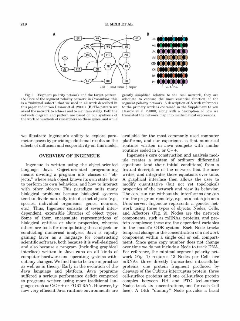
Fig. 1. Segment polarity network and the target pattern.(A) Core of the segment polarity network in Drosophila; thisis a ‘‘minimal subset’’ that we used in all work described inthis paper and in von Dassow et al. (2000). (B) The pattern weasked the network to achieve and to maintain stably. Both thenetwork diagram and pattern are based on our synthesis ofthe work of hundreds of researchers on these genes, and while

greatly simplified relative to the real network, they areadequate to capture the most essential function of thesegment polarity network. A description of A with referencesto the primary work is contained in the Supplement to vonDassow et al. (2000), along with a description of how wetranslated the network map into mathematical expressions.

E. MEIR ET AL.218

transcriptional input to the Node ci (whichrepresents the cubitus interruptus mRNA). InFigure 1, Nodes are represented by oval icons formRNAs, rectangular icons for directly transcribedproteins and their cleavage products, and hexago-nal icons for dimers/polymers of those proteins.

Each cell in an epithelial sheet corresponds toone of Ingeneue’s Cell objects, which stores acomplete set of that Cell’s Nodes in the networkalong with the identities of each neighboring Cell.Epithelial layers in developing Drosophila em-bryos (and many other species as well) generallyconsist of polygonal cells with roughly six sides.The issue of how cell shape affects patterning isworth exploring, but currently, for simplicity, werepresent Cells in Ingeneue as two-dimensionalregular hexagons that do not move. No constraintinherent in Ingeneue’s design prevents us fromeventually adding a more sophisticated represen-tation of cells, sheets of cells, movement of cellswithin sheets, and mitoses. Each Ingeneue Cellhas seven compartments: a ‘‘cytoplasmic/nuclear’’compartment, where all intracellular Nodes re-side, and six ‘‘membrane’’ compartments, one foreach side of the cell. Ingeneue tracks concentra-tions of membrane-bound components (for in-stance trans-membrane ligands and receptorssuch as WG, PTC, HH, and PH in Fig. 1)separately for each cell face, and each pair ofneighboring cell faces interact independently.Ingeneue allows these membrane-bound compo-nents to flow from each side of a cell to the twoneighboring sides of the same cell. Ingeneue alsoallows exchange between apposite faces of neigh-boring cells. Together, these two features allowmolecules to ‘‘diffuse’’1 across the sheet of cells(Fig. 2, middle panel). Ingeneue can easily accom-modate other notions of cell compartmentalizationwhich certain other applications may require.

Ingeneue uses arrays of hexagonally packedcells (Fig. 2). In the current version, boundarieswrap around both horizontally and verticallyso, for instance, the left-hand neighbor of a cell

Fig. 2.

1Ingeneue does not do ‘‘real’’ diffusion, that is, concentration-dependent flux governed by a partial differential equation parameter-ized by D, hence the quotation marks. However the face-to-faceexchange mechanism corresponds to a coarse discretization of a fluxequation, and serves adequately for any purpose we have yetencountered. In any case, we doubt that free diffusion, per se, isrealistic for most molecules expressed in embryonic tissues of animals;rather, most secreted proteins probably associate with the cell surfaceand extracellular matrix to greater or lesser degrees, and thusIngeneue’s mechanism seems to us more satisfying. It is also moreuseful because it subsumes all the buzzwords: autocrine, paracrine,and juxtacrine signaling, as well as free diffusion, can be achievedwithin different parameter regimes.


on the left edge is a cell on the right edge. Ourwrap-around boundaries, which give our cellsheets the topology of a torus, remove boundaryeffects. This is an advantage for spatially periodicpatterns such as those the segment polaritynetwork typically makes. In cases where wrap-around boundaries are inappropriate, we add anextra strip of ‘‘dead’’ cells around the edge of thesheet with initial conditions that cause them notto participate in the patterning process beingmodeled. The initial segment polarity pattern iscomposed of stripes, perpendicular to the ante-rior–posterior axis, that repeat every four cells, sofor the crudest applications using this network wecan get away with a 4�1 rectangle of cells.

A major advantage of using Ingeneue for geneticnetwork modeling is that the user need specify thenetwork in a typical cell only once. Ingeneue doesthe drudgery of instantiating the network intoeach Cell in the model and setting up theappropriate relations between neighboring cells.Thus in Figure 2, there are only three componentswe need to specify: wg (mRNA) and I-WG (protein)in the intracellular compartment; and E-WG

(protein) in the cell surface compartment. Thereare four interactions: wg-I-WG (translation); I-WG2E-WG (bi-directional exchange betweencompartments); the flux rate of E-WG aroundthe cell periphery; and the flux rate of E-WG fromcell to cell. This is much faster and more reliablethan enumerating the ODE system by hand, asone would have to do absent a tool like Ingeneue:imagine typing out all 120 ODEs (with allconnections represented by 870 additive terms,carefully indexed to appropriate Cell and Cell face)required for the 15-cell grid at the top of Figure 2!For a realistic problem, such as the minimalsegment polarity model in a mere 4� 1 cell grid,the use of a standard symbolic mathematicspackage would require the user to type out asystem of nearly 140 coupled ODEs. Ingeneuereduces this to 13, uses stereotyped building blocks,Affectors, to construct the differential equations,and can expand that 4�1 grid to arbitrary size byediting just two numbers in the input file.

Affectors represent the interactions betweenNodes. Each Affector encapsulates a formulacorresponding to a physical process involving oneor more Nodes. Each Node computes the rate ofchange in its concentration (its time derivative) bycombining the values all its Affectors contribute.Table 1 illustrates the four conceptual groups thatmost of Ingeneue’s Affectors fall into. SomeAffectors govern synthetic processes such astranscription and translation. A second groupgoverns non-specific first-order decay of eachmolecule. A third group represents transforma-tions of proteins from one form to another (viareactions such as cleavage and hetero-dimeriza-tion), some of which may be reversible. The fourthgroup mediates exchange of molecules betweendifferent compartments within and among cells.Ingeneue currently includes approximately 60Affectors (all in dimensionless form, as describedin the supplement to von Dassow et al., 2000;future editions will include complementary di-mensional-form building blocks) that we devel-oped to construct our segment polarity andneurogenic network models. These provide aversatile, expanding basis for constructing modelsof similar ‘‘resolution’’ and complexity to oursegment polarity model. Furthermore, it is asimple Java programming task to create a newAffector type, especially given the existinglibrary as exemplars. This is a key feature of ourdesign goals for Ingeneue: it should be easy for abiologist possessing an acquaintance with themathematics and only a little familiarity with

Fig. 2 is on page 219

Fig. 2. Pieces of an Ingeneue model. (A) Ingeneue modelsare made of Cells, Nodes, and Affectors. Cells are hexagonalwith one cytoplasmic compartment and six membranecompartments. Cells are arranged in a grid, with each faceof a Cell in contact with a face of one of its neighbors. Cell faceson the edges of the grid are wrapped around as if on a torus tobe in contact with ‘‘neighbors’’ on the opposite side of the grid.All Cells contain identical copies of a network, where thenetwork is composed of Nodes (that is, molecular species; ovalsand polygons in middle panel) and Affectors (arrows in middlepanel, boxes in lower panel). The middle panel shows a subsetof the Nodes and Affectors from the segment polarity network.Transcription of the wg mRNA produces an internal WGprotein pool (I-WG). This internal WG pool exocytoses ontoeach face of the Cell (E-WG), from whence it can exchange tothe apposite faces of neighboring cells or to neighboring facesof the same cell. Endocytosis transfers E-WG, at a rateproportional to its concentration on each Cell face, to I-WG.Combined, these exchange processes subsume, in differentregions of parameters space, autocrine, paracrine and juxta-crine signaling, transcytosis, and even ‘‘free diffusion.’’ Thebottom panel shows the four Affectors that are summedtogether to compute the time rate of change in I-WGconcentration. They represent, from left to right, translationof I-WG from wg mRNA, exocytosis to the membrane,endocytosis from the membrane, and non-specific decay. (B)The ‘‘sheet-of-hexagons’’ approximation is not so unrealistic;in many developing embryos, such as the neurula-stageascidian embryo shown here in a scanning electron micro-graph provided by G. von Dassow, pattern formation takesplace in epithelial sheets in which the cells are roughlyhexagonally packed.

3

E. MEIR ET AL.220

Java programming to extend Ingeneue to accom-modate a wide variety of similar gene networkmodeling tasks.

For some processes we use Affector formulaethat represent the exact chemistry involved;examples include first-order reactions like decayand second-order reactions such as ligand binding.In other instances we only approximate the literalkinetic process. The most common approximationwe adopt is to use generic Hill-function-likesigmoid curves to model how transcription factorswork. We digress a moment to explain that we useapproximations because we prefer formulae thatcorrespond to a biologist’s description of a genenetwork quantified by parameters which, inprinciple, biologists could measure experimen-tally. For instance, in most contexts a biologistexplaining how a group of genes regulate eachother would not detail all the steps of transcriptionfactor binding and sequential assembly of thegeneric transcriptional machinery. Instead shewould say things like, ‘‘Engrailed represses cubi-tus interruptus transcription.’’ The details of howit does so, even though they might be veryinteresting, often remain unknown. What onedoes know is that every target gene has somemaximal rate of transcription. That maximal rate,

determined by enzymatic properties of RNApolymerase and by how suitable a template thegene in question makes, provides one parametergoverning the synthesis rate function for thatgene. Saturation at a maximal rate implies that,for every regulator, there is some regulator level atwhich the target achieves one-half its maximalsynthesis rate. That half-maximal level providesanother parameter.

The functional form quantifying the dose–response relation between a transcription factorand the transcription rate it modulates must benonlinear if that rate saturates. The next practicalissue is, how sharply nonlinear is the dose–response curve? Thus a third parameter deter-mines the slope of the dose–response curve at thehalf-maximal point. An inflected dose–responsecurve could arise, for example, from cooperativebinding effects, with steeper curves resulting fromhigher-order complex formation. This reasoningled us to adopt the kind of curve and parametersshown in Figure 3, combinations of which In-geneue uses to model transcriptional regulatoryinteractions and other dose–response relation-ships. By neglecting to explicitly represent theassembly of the generic transcriptional machinerywe assume that this process is not a rate-limiting

TABLE1. Ingeneue’s classes of a¡ectors1

A¡ector type Description Examples

Synthesis Transcription of mRNAs andtranslation of mRNAs into proteins

To

Hx

Y �Yx

K�YxYx þ Y �Yx

� �To

Hx

A�Ax

K�AxAx þ A�Ax

� �1 � I�Ix

K�IxIx þ I�Ix

� �

Decay First-order generic, nonspeci¢c decaythat (usually) a¡ects all Nodes.

� X

HX

Transformation Changes of one Node Into another,e.g., cleavage, phosphorylation, dimerization, etc.

ToYo �kXþY!XYXYð Þ

� CYXXTo

HX

Y �YX

K�YXYX þ Y �YX

� �

Transfer Various exchanges: of membrane-boundNodes among cell faces, between cells,endo- and exocytosis, etc.

rflux of X Xopposite face � Xthis face

� �

1We combine each A¡ector’s formula into the right hand side of the ODE that speci¢es the time rate of change of a Node’s concentration. Under‘‘Synthesis’’ the exhibited formulae confer transcription regulated by a single activator, and transcription regulated by a single activator andsingle global repressor. An a¡ector from the ‘‘Decay’’category is usually added to every component of the model. Although Ingeneue never checks,it is usually important to include a non-speci¢c decay term for every Node. Since this term is linearly dependent on the concentration of the Node,and all synthetic processes should saturate to be biologically realistic, the decay term ensures a maximal steady state level for every Node. Under‘‘Transformation’’ the ¢rst formula represents hetero-dimerization between X andY, while the second gives the rate of cleavage (or some other trans-formation) of X regulated byY. Under ‘‘Transfer’’ the exhibited formula confers exchange between the apposite faces of two neighboring cells. In factthis formula is represented by an obligate pair of A¡ectors, thus maintaining a one-to-one relationship between A¡ectors and additive terms in theODE. See the Supplement to von Dassow et al. (2000) for a rationalization of the formulas used and the non-dimensionalization scheme.


step. The major constraint we maintain is that alltranscription must saturate at some maximallevel; thus we never use linear or strictly additiveformulas. But we emphasize that Ingeneue itselfenforces no constraints whatever on an Affector’sformula, so others could make different choices.2

The most mathematically complex Affectors arethose governing transcription. This reflects theinherent complexity of the transcription process.Multiple transcription factors activate/inhibitmost enhancer regions through detailed interac-tions we do not know. As explored further inAppendix A, various nested or multiplicativecombinations of sigmoid dose–response curves likeFigure 3 accommodate most of the possibilities forsimple relationships between regulators and tar-gets. In cases where only a single activator acts ona target gene, we use the simple parametrizedsigmoid function in Figure 3 to quantify thetranscription rate. To add a single inhibitor wemight choose to multiply the activation functionby one minus a similar function (Table 1). Even insuch a simple one activator/one inhibitor case wenecessarily make assumptions about the physicalmechanism of inhibition. With multiple activatorsand inhibitors, the potential combinations geteven more complicated. Ingeneue presently in-cludes the rudiments of a flexible system using‘‘meta-affectors’’ that add and multiply togethersimple activation and inhibition formulas whilestill preserving an overall maximum transcriptionrate for the target gene.

Partitioning the equations for a network modelinto stereotyped, reusable function fragments isanother major advantage of using Ingeneue formodeling genetic networks. The Affectors consti-tute a parts kit for translating the cross-regulatoryconnections in a typical network diagram, such asFigure 1, into a set of ODEs representing thoseconnections mathematically. This tactic enablesusers to build and modify a network modelwithout needing to derive equations themselvesfor each case. (Nevertheless, it is vital that usersunderstand the generic nature of the kinds ofODEs that Ingeneue uses and understand howeach choice differs mechanistically.) This tacticalso greatly speeds up the process of changingnetwork topologies, even for mathematically so-phisticated users.

Fig. 3. Standard dose–response curve. This S-shapedcurve, a graph of the key term in the differential equationshown above, is a fundamental approximation for regulatoryrelationships in Ingeneue. The equation in this figure is asimple case in which synthesis of X is promoted by Y, and Xdegrades non-specifically. The curve represents the rate ofsynthesis of X as a function of Y, absent decay. A salientfeature is that at high activator concentration, the responsesaturates at some maximal value, determined by the proper-ties of the biosynthetic machinery (e.g., RNA polymerase). Itfollows that at some intermediate activator concentration (KY)the response reaches half its maximal value. Throughout,when we use the word ‘‘cooperativity’’ we are really referringto the steepness of the curve at the inflection point (since suchan inflection could be produced by cooperative interactionsamong activator molecules). The thumbnail curves showidentically scaled versions with the cooperativity equal to1.0, 4.0, and 10.0. With a cooperativity of 1.0 (that is, nocooperativity) the dose–response curve is nearly linear at lowregulator concentrations, has no inflection, and saturatesmore slowly than corresponding curves with higher n. With acooperativity above 10.0 or so, the curve is nearly a stepfunction. In Ingeneue models the half-maximal activationvalue and the cooperativity become free parameters of thisformula, but the equations are normalized and rendereddimensionless such that, for processes like transcription, themaximal rate is 1.0. An inhibitory dose–response curve is thusobtained by subtracting a formula for the curve shown from1.0. Complicated terms, such as would govern transcriptionalregulation by several factors, are obtained by nesting, adding,and multiplying these curves in various combinations deter-mined by the mechanism in question.

2Since there is an infinitude of monotone-increasing functionshaving a given maximum, a given half-maximal point, and a givenslope there, we do not believe that it is worthwhile to distinguish them.Convenience and tradition dictated the choice of a Hill function, butIngeneue would just as happily integrate anything else.

E. MEIR ET AL.222

Creating a model of a gene network usingIngeneue thus consists of specifying the Nodes,Affectors, and the size and geometry of the Cellarray. In order to do anything with that topologyone must assign values to all the Affectors’parameters and to the initial concentrations ofeach Node in each Cell. Then Ingeneue ‘‘runs’’ themodel by integrating the equations over a user-specified time interval. Running the model pro-duces dynamic behavior, visible on the computerscreen as well as measurable within the program’sguts, which we generally want to compare to geneexpression patterns in the real biological system.The network’s behavior, and the final state thatthe pattern may approach after long times (if sucha state exists), depend on all the model’s ingre-dients and initial conditions. This behavior may besensitive to any particular ingredient, or mayhardly be sensitive to any of them, and clearlycould depend a great deal on governing parametervalues. We now describe some of Ingeneue’s toolsfor exploring those dependencies.

WANDERING THROUGHHIGH-DIMENSIONAL PARAMETERSPACE SEEKING ZONES IN WHICH

MODEL NETWORKS EMULATEREAL NETWORKS

In the classical context of genetics, each gene’seffects on phenotype characterize its function; onefunction of wingless, for instance, is to specifyregions of naked cuticle in each segment duringembryogenesis. In the context of molecular genet-ics, gene function means how the gene productinteracts with other genes and their productswithin some pathway or program. That is, thefunction of wingless is to respond to certain intra-and inter-cellular signals and transmit them tocertain targets. How does one ascribe a function toa network of genes? Going from individual genesto networks, it seems sensible to try abstractingfunctional ‘‘behaviors,’’ much as one would do tocomprehend integrated circuit chips. One functionof the segment polarity network is to do a certaintask, and the question is, what task?3

A simplistic description of the segment polaritynetwork’s task in early Drosophila development isto sharpen initial condition cues, conferred by thetransiently-expressed pair rule genes, into theparasegmental boundaries, and then maintainthese boundaries (in a subset of the animal)

throughout development. The boundaries aredefined by expression of the network’s constituentgenes in a particular stable spatial pattern.Another way of saying this is that if somehow wecould make a naı̈ve field of cells capable ofexpressing only the segment polarity genes (andall the generic machinery for basic cell function),and if somehow we could provide an initial pre-pattern equivalent to the input they usually getfrom pair-rule genes, we would expect this net-work to stably maintain an asymmetric spatialregime of gene expression. That, we propose, is thefunction of this network. Ingeneue allows one todo this experiment in silice.4 One can reconstitutea working circuit from the parts list deciphered bymolecular geneticists and inquire whether thatcircuit indeed does the task it is supposed to do.Incidentally, we find the abstraction of a net-work’s functional task one of the most difficult(and most critically vulnerable) parts of the entiremodeling process. Given a group of genes thatinteract, how are we to characterize what it is thatthey do, and which aspects of what they areobserved to do, are the important aspects?

No matter how difficult it is to deduce thefunction of a specific network, that functionusually abstracts to some dynamical behavior,such as producing a pattern of gene expression intime, space, or both. The spatiotemporal patternthat emerges depends not only on the network’stopology but also on the values of parameters inthe model and on the initial conditions. Theseparameters quantify the shapes and strengths ofthe network’s connections by specifying biochem-ical reaction rates for translation, degradation,dimerization, and so on. Exploring how a net-work’s behavior may (or may not) change asparameter values change is the central, inescap-able task of all gene network modelers (untilactual values for all the parameters have beenmeasuredFthus, realistically, forever or at leastuntil all authors of this paper have passed away).Even the simplest realistic networks involveextravagant numbers of parameters (48 in Fig.1). This is not a calamity caused by mathematical

3Of course the same network may have other functions at differentdevelopmental stages, or in a different organism.

4The term ‘‘in silico’’ has become commonplace in the last severalyears, but after we used it in von Dassow et al. (2000), Reed A.Cartwright wrote us as follows:

‘‘I would like to point out an error in your paper. You used the term‘‘in silico’’ to compare computational simulations to that of life (invivo) and laboratory (in vitro). However, you have made a mistake inyour Latin. Silicon comes from the Latin word silex which means‘‘hard stone.’’ Unlike vivus and vitrum which are second declentionnouns, silex is a third declention noun, and thus its ablative singular issilice. And since ‘‘in’’ takes the ablative, the correct phrase for ‘‘instone’’ would be in silice and not in silico.’’


modeling, but a fact of nature, a fact whichmathematicians cannot but sin to gloss over. Formuch simpler networks than Figure 1 it is possibleto exhaustively catalog a network’s behavioracross all biologically realistic parameter combina-tions, but this is out of the question for almostanything interesting. If we assign each parametereither a high, medium, or low value, it wouldrequire roughly 348, or E8� 1022, samples to tryevery possible combination in the segment polar-ity network. Waiting (e.g., for AMD to release theAthlon XII) will never make it realistic to do atenth of a mole of simulation runs. Our labor-atory’s existing computers could perform thenecessary calculations in 1014 years. So, sinceexhaustive exploration is right out, one hasroughly four choices:

K Use mathematical strategies for dealing withlarge parameter spaces, such as non-linear opti-mization techniques that start from a guessed setof parameter values and search iteratively fornearby parameter values that better match thetarget behavior;

K Constrain the problem using empirical informa-tion, such as the knowledge that transcriptionfactor X is a potent activator of gene y but a pooractivator of gene z, or that protein A is much morerapidly degraded than protein B;

K Intuit what values will make the network performits ‘‘function’’;

K Depend upon the luck to model a network whoseconnection topology, we presume, natural selec-tion has optimized over deep time to have the

mysterious property that it is trivially easy tofind, by accident, sets of parameter values thatconfer the desired behavior on the network.

We confess to relying primarily, though notexclusively, on the fourth option, after discoveringthis unforeseen but happy possibility. As men-tioned above, for the segment polarity networkmodel we were able to find ‘‘good’’ parameter setsthat caused the network to make a reasonablematch to Figure 1B merely by randomly choosingvalues for each parameter. Naming mathematicalparameters that confer shape and strength onnetwork connections, then seeking ‘‘good’’ valuesfor them, may seem artificial mumbo jumbo withwhich mathematical modelers merely confuse analready difficult problem. But it is not so: regard-less of what jargon one uses to describe theformidable task of navigating high-dimensionalparameter spaces, performing that task is thelikely operation of evolution by natural selection.

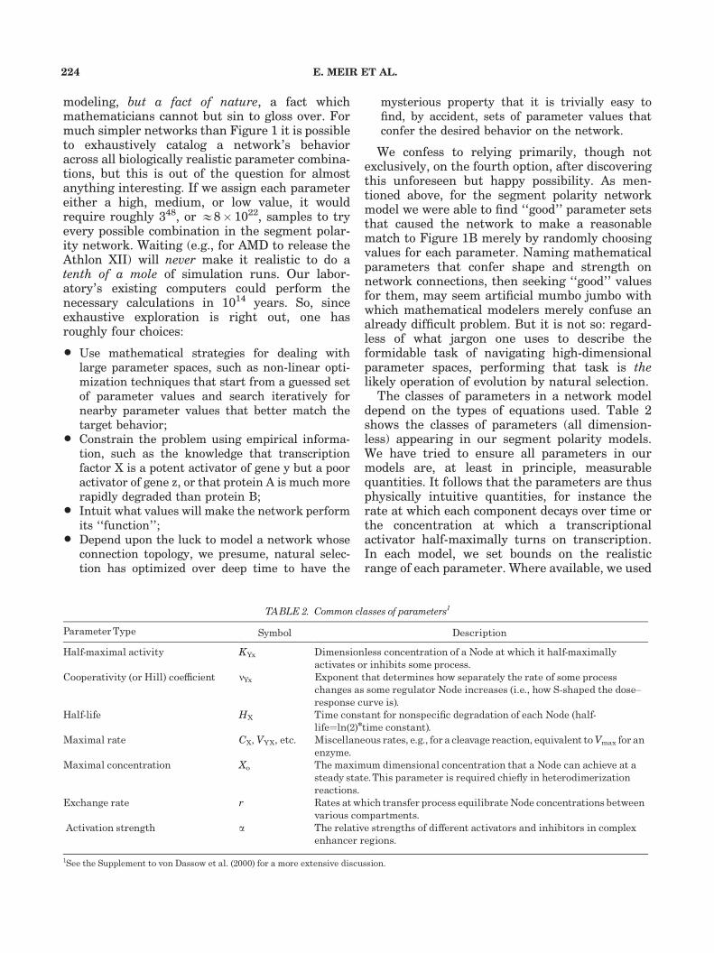
The classes of parameters in a network modeldepend on the types of equations used. Table 2shows the classes of parameters (all dimension-less) appearing in our segment polarity models.We have tried to ensure all parameters in ourmodels are, at least in principle, measurablequantities. It follows that the parameters are thusphysically intuitive quantities, for instance therate at which each component decays over time orthe concentration at which a transcriptionalactivator half-maximally turns on transcription.In each model, we set bounds on the realisticrange of each parameter. Where available, we used

TABLE 2. Common classes of parameters1

ParameterType Symbol Description

Half-maximal activity KYx Dimensionless concentration of a Node at which it half-maximallyactivates or inhibits some process.

Cooperativity (or Hill) coe⁄cient nYx Exponent that determines how separately the rate of some processchanges as some regulator Node increases (i.e., how S-shaped the dose^response curve is).

Half-life HX Time constant for nonspeci¢c degradation of each Node (half-life¼ln(2)ntime constant).

Maximal rate CX, VYX, etc. Miscellaneous rates, e.g., for a cleavage reaction, equivalent toVmax for anenzyme.

Maximal concentration Xo The maximum dimensional concentration that a Node can achieve at asteady state.This parameter is required chie£y in heterodimerizationreactions.

Exchange rate r Rates at which transfer process equilibrateNode concentrations betweenvarious compartments.

Activation strength a The relative strengths of di¡erent activators and inhibitors in complexenhancer regions.

1See the Supplement to von Dassow et al. (2000) for a more extensive discussion.

E. MEIR ET AL.224

published values as guides to the general rangeand then expanded bounds to span the smallestand largest biologically reasonable values. As anexample, in exploring the segment polarity net-work we let what we call ‘‘half-lives’’ (thedegradation time constants, actually) vary be-tween 5 and 100 min. We considered it unlikelythat these molecules were degraded much morerapidly than with a 5-min time constant (corre-sponding to a half-life of about 3 min, about whathas been measured for ftz mRNA; Edgar et al.,’86). At the upper end, the segment polaritypattern forms over the course of hours or less, sothe gene products involved must degrade fastenough to change on that time scale. We thus setthe upper limit on degradation time constants at100 min. Published measurements of half-lives inthe segmentation network all fall within thisrange: Engrailed protein has a half-life ofo15 min (Weir et al., ’88); Armadillo protein(involved in segmentation though not explicitlyrepresented in the model discussed here) has ahalf-life of around 12 min (Pai et al., ’97); Cubitusinterruptus protein, in cultured cells, has a half-life of 75 min (Aza-Blanc et al., ’97).

Automating the search for ‘‘working’’ sets ofparameter values requires a goodness-of-fit func-tion which we craft to assess how close thenetwork, with each trial parameter set, comes tomatching the target behavior. Pattern matching iscurrently the weakest part of Ingeneue in terms ofmaking a program that can be used by biologistswithout additional customization, and we do notyet have a full solution. Presently the user mustcustom-code their own pattern recognizer if thosewe supply do not suit the task. It is much less clearin the case of pattern recognition than it is for theAffectors what the primitive unit for generalapplications should be, so to date we have suppliedvery few. The general strategy in Ingeneue is toallow the user to assemble, from a library ofprimitive parts or by custom coding, so-called‘‘StoppingCondition’’ objects. StoppingConditionobjects monitor the progress of the integration runand return a scalar score measuring how well therun conforms to some ideal behavior, and they canbe set up to suspend the run if it is pointless tocontinue further (i.e., if either the network hasalready conformed well enough to the idealbehavior, or if it is clear that it will never conform,say, because it has achieved some alternate stablestate). Our current StoppingConditions can lookfor primitive behaviors such as ‘‘Node X on in Cell1,’’ ‘‘Node X off in Cell 2,’’ and ‘‘Node Y oscillating

in Cell 3.’’ We then combine several StoppingCon-ditions together to recognize more complex pat-terns.

For example, the target pattern for the segmentpolarity network is a set of vertical stripes: a stripeof en in the first column of each parasegmentalrepeat, a stripe of wg in the fourth column, a stripeof hh where en is on, and so on. Our patternrecognizer function for the segment polarity net-work is thus a group of several StoppingCondi-tions that recognize stripes. Together these assesswhether the model achieves the correct on/offpattern of wg, en, and hh, in the desired positionsand in a sufficiently short time (see Supplement tovon Dassow et al., 2000). The stripe recognizerreturns a better (lower) score as the differencebetween the concentrations within that columnand in neighboring columns grows larger, and itsscore also improves if the concentration within thecolumn is stable over time. We laboriously hand-tuned the exact recipe for the segment polaritymodel’s pattern recognizer function until it caughtonly the parameter sets we wanted. We doubt thatwe will ever be able to eliminate the need for suchhand-tuning, but the challenge for future devel-opment of this aspect of Ingeneue is to incorporatea versatile library of pattern recognizer modulesthat allow one to avoid custom coding for mostapplications.

Given a function that scores patterns, Ingeneuecan automatically search parameter space for setsof parameter values that produce that pattern(i.e., that achieve a sufficiently low value of the‘‘objective function’’ which measures distanceaway from the ideal pattern). This is anothermajor advantage of using Ingeneue to build andanalyze gene network models. The basic frame-work for automated searching is a collection of‘‘Iterator’’ objects. We have been rather surprisedto find that so far, for several different cases, themost useful algorithm has been random samplingof parameters from within biologically realisticranges of parameter values. Other Iteratorsimplement various algorithms for navigating thelandscape in parameter space, including a varietyof standard and custom-made nonlinear optimiza-tion schemes. Because most of our work to datehas, fortuitously or otherwise, allowed us to takethe most simple-minded of approaches, we haveyet to explore thoroughly the effectiveness ofvarious sophisticated strategies for searchingparameter space. We expect, however, that sincethese network models all use similar equations,it should be possible to identify which search


algorithms work best on this whole class ofmodels. Once (or if) one finds sets of parametervalues for which the model works, the Iteratorframework enables automated sensitivity tests.For example, Figure 3 of von Dassow et al. (2000)was made using the ‘‘TransectIterator’’ object,which, starting with an input parameter set,simply scans along the entire range of one ormore parameters while keeping all other para-meter’s values fixed and records the score at eachpoint. Again, Ingeneue’s design allows one to add,as a drop-in module, any stratagem one wants totry.

USING INGENEUE WITH A MOUSE

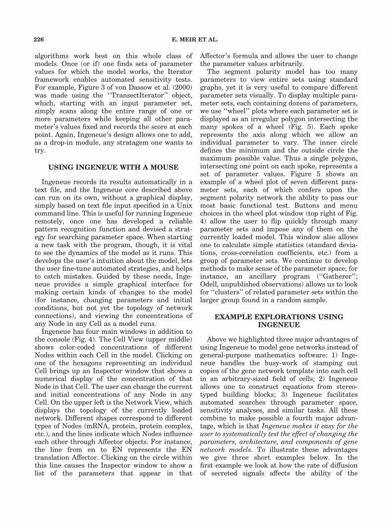
Ingeneue records its results automatically in atext file, and the Ingeneue core described abovecan run on its own, without a graphical display,simply based on text file input specified in a Unixcommand line. This is useful for running Ingeneueremotely, once one has developed a reliablepattern recognition function and devised a strat-egy for searching parameter space. When startinga new task with the program, though, it is vitalto see the dynamics of the model as it runs. Thisdevelops the user’s intuition about the model, letsthe user fine-tune automated strategies, and helpsto catch mistakes. Guided by these needs, Inge-neue provides a simple graphical interface formaking certain kinds of changes to the model(for instance, changing parameters and initialconditions, but not yet the topology of networkconnections), and viewing the concentrations ofany Node in any Cell as a model runs.

Ingeneue has four main windows in addition tothe console (Fig. 4). The Cell View (upper middle)shows color-coded concentrations of differentNodes within each Cell in the model. Clicking onone of the hexagons representing an individualCell brings up an Inspector window that shows anumerical display of the concentration of thatNode in that Cell. The user can change the currentand initial concentrations of any Node in anyCell. On the upper left is the Network View, whichdisplays the topology of the currently loadednetwork. Different shapes correspond to differenttypes of Nodes (mRNA, protein, protein complex,etc.), and the lines indicate which Nodes influenceeach other through Affector objects. For instance,the line from en to EN represents the ENtranslation Affector. Clicking on the circle withinthis line causes the Inspector window to show alist of the parameters that appear in that

Affector’s formula and allows the user to changethe parameter values arbitrarily.

The segment polarity model has too manyparameters to view entire sets using standardgraphs, yet it is very useful to compare differentparameter sets visually. To display multiple para-meter sets, each containing dozens of parameters,we use ‘‘wheel’’ plots where each parameter set isdisplayed as an irregular polygon intersecting themany spokes of a wheel (Fig. 5). Each spokerepresents the axis along which we allow anindividual parameter to vary. The inner circledefines the minimum and the outside circle themaximum possible value. Thus a single polygon,intersecting one point on each spoke, represents aset of parameter values. Figure 5 shows anexample of a wheel plot of seven different para-meter sets, each of which confers upon thesegment polarity network the ability to pass ourmost basic functional test. Buttons and menuchoices in the wheel plot window (top right of Fig.4) allow the user to flip quickly through manyparameter sets and impose any of them on thecurrently loaded model. This window also allowsone to calculate simple statistics (standard devia-tions, cross-correlation coefficients, etc.) from agroup of parameter sets. We continue to developmethods to make sense of the parameter space; forinstance, an ancillary program (‘‘Gatherer’’;Odell, unpublished observations) allows us to lookfor ‘‘clusters’’ of related parameter sets within thelarger group found in a random sample.

EXAMPLE EXPLORATIONS USINGINGENEUE

Above we highlighted three major advantages ofusing Ingeneue to model gene networks instead ofgeneral-purpose mathematics software: 1) Inge-neue handles the busy-work of stamping outcopies of the gene network template into each cellin an arbitrary-sized field of cells; 2) Ingeneueallows one to construct equations from stereo-typed building blocks; 3) Ingeneue facilitatesautomated searches through parameter space,sensitivity analyses, and similar tasks. All thesecombine to make possible a fourth major advan-tage, which is that Ingeneue makes it easy for theuser to systematically test the effect of changing theparameters, architecture, and components of genenetwork models. To illustrate these advantageswe give three short examples below. In thefirst example we look at how the rate of diffusionof secreted signals affects the ability of the

E. MEIR ET AL.226

segment polarity network to produce the patternin Fig 1B. In the second example we ask the samequestion but with respect to the degree of‘‘cooperativity’’ in regulatory interactions in thenetwork. Finally we illustrate how the segmentpolarity module really consists of two sub-mod-ules.

Sensitivity of the segment polarity modelto diffusion rates

There is a long-standing controversy concerningthe role diffusion plays in developmental patternformation. It has proven difficult to demonstrateconclusively that diffusion gradients of proteins

actually exist, or that these gradients affectpatterning. In part, this experimental quest tofind diffusing molecules was driven by a body ofmathematical theory that assumed diffusion ofmolecules was centrally important in patterning(Slack, ’83; summarized in Murray, ’93). Thetheory is based on Turing’s idea of reactionsamong competing proteins that diffuse at differentrates. Depending on the types and rates of thereactions and the rates of diffusion, various simplemodels can exhibit interesting pattern-formingbehaviors. One of the primary difficulties withthese so-called reaction–diffusion mechanisms,however, is that they generally require carefultuning of relative reaction rates versus the

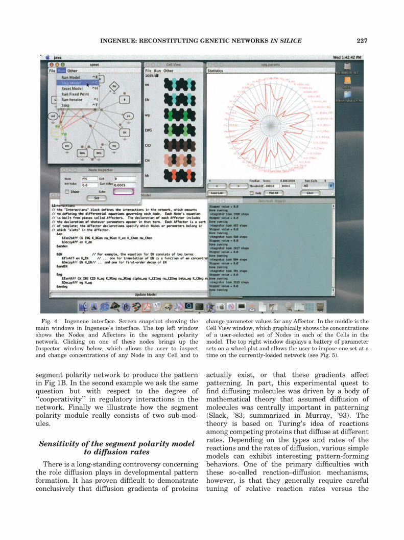
Fig. 4. Ingeneue interface. Screen snapshot showing themain windows in Ingeneue’s interface. The top left windowshows the Nodes and Affectors in the segment polaritynetwork. Clicking on one of these nodes brings up theInspector window below, which allows the user to inspectand change concentrations of any Node in any Cell and to

change parameter values for any Affector. In the middle is theCell View window, which graphically shows the concentrationsof a user-selected set of Nodes in each of the Cells in themodel. The top right window displays a battery of parametersets on a wheel plot and allows the user to impose one set at atime on the currently-loaded network (see Fig. 5).


diffusion rates. In particular, the ‘‘wavelength’’ ofthe patterns made by reaction–diffusion mechan-isms is highly sensitive to the rates at whichvarious factors diffuse across the simulated field.

Several recent studies demonstrate that devel-opmentally important molecules do indeed diffusefrom their site of synthesis, and that the concen-tration gradients thus established play a role inpatterning (see for example Gurdon et al., ’94, andNellen et al., ’96). Two of the segment polaritynetwork components, Wingless and Hedgehog, aresecreted proteins that potentially spread throughthe embryonic epidermis by diffusion (or even byconvection or active transport of some kind).However, we do not know if diffusion of thesesignals influences the segment polarity network’sfunction in vivo. Both Wg and Hh transport arecarefully regulated in fly embryos. There issubstantial evidence that during embryogenesis

the primary means by which Wg travels from cellto cell is an active transport mechanism involvingendocytic uptake (Dierick and Bejsovec, ’98; Mo-line et al., ’99; Pfeiffer and Vincent, ’99), and itremains unclear to what extent (if any) theappearance of Wg protein far from its site ofsynthesis is due to genuine extracellular diffusion.Hh is synthesized as a transmembrane precursorand undergoes autolytic processing to a cholester-ol-tethered form whose cell-to-cell transport maybe mediated by other regulators, such as Patchedand Dispatched (Burke et al., ’99). This suggeststhat Hh transport might be under tight controlin vivo, but introduction of a freely diffusible Hhhas only subtle effects on embryogenesis (Porteret al., ’96).

During our initial work with the segmentpolarity model we allowed the Wingless ‘‘diffu-sion’’ rate to vary over a wide range, from values

Fig. 5. Wheel plot. Wheel plots exhibit multiple parametersets, each comprising dozens of parameters. Each spoke is theaxis (log or linear scale, as chosen by the user) for one of the 48parameters in the model. The inner circle represents theminimum value in each parameter’s range, and the outercircle represents the maximum value. Thus one parameter setis represented by a single irregular polygon with a vertex oneach spoke of the wheel. The dashed polygon is one parameter

set that was successful at forming the segment polaritypattern. The other six polygons show other successfulparameter sets. Notice that each of these has very differentparameter values from the others. By plotting many para-meter sets on top of each other, one can get an idea of whetherone or another parameter’s values are clustered in one part ofits range.

E. MEIR ET AL.228

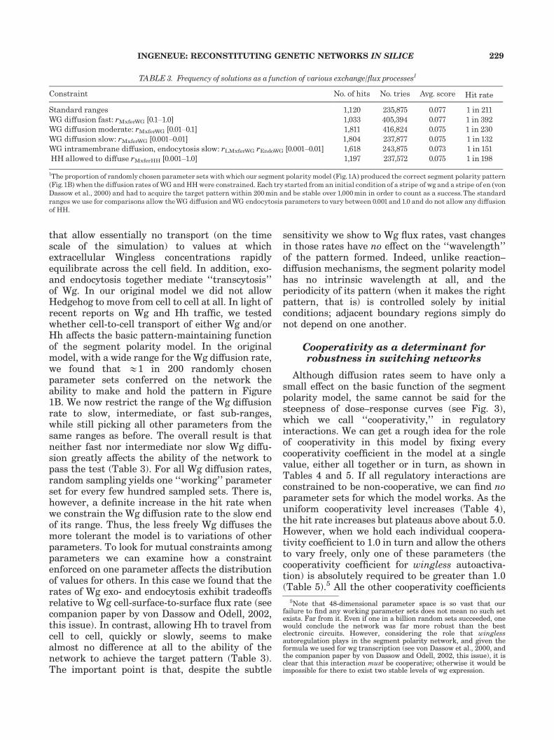
that allow essentially no transport (on the timescale of the simulation) to values at whichextracellular Wingless concentrations rapidlyequilibrate across the cell field. In addition, exo-and endocytosis together mediate ‘‘transcytosis’’of Wg. In our original model we did not allowHedgehog to move from cell to cell at all. In light ofrecent reports on Wg and Hh traffic, we testedwhether cell-to-cell transport of either Wg and/orHh affects the basic pattern-maintaining functionof the segment polarity model. In the originalmodel, with a wide range for the Wg diffusion rate,we found that E1 in 200 randomly chosenparameter sets conferred on the network theability to make and hold the pattern in Figure1B. We now restrict the range of the Wg diffusionrate to slow, intermediate, or fast sub-ranges,while still picking all other parameters from thesame ranges as before. The overall result is thatneither fast nor intermediate nor slow Wg diffu-sion greatly affects the ability of the network topass the test (Table 3). For all Wg diffusion rates,random sampling yields one ‘‘working’’ parameterset for every few hundred sampled sets. There is,however, a definite increase in the hit rate whenwe constrain the Wg diffusion rate to the slow endof its range. Thus, the less freely Wg diffuses themore tolerant the model is to variations of otherparameters. To look for mutual constraints amongparameters we can examine how a constraintenforced on one parameter affects the distributionof values for others. In this case we found that therates of Wg exo- and endocytosis exhibit tradeoffsrelative to Wg cell-surface-to-surface flux rate (seecompanion paper by von Dassow and Odell, 2002,this issue). In contrast, allowing Hh to travel fromcell to cell, quickly or slowly, seems to makealmost no difference at all to the ability of thenetwork to achieve the target pattern (Table 3).The important point is that, despite the subtle

sensitivity we show to Wg flux rates, vast changesin those rates have no effect on the ‘‘wavelength’’of the pattern formed. Indeed, unlike reaction–diffusion mechanisms, the segment polarity modelhas no intrinsic wavelength at all, and theperiodicity of its pattern (when it makes the rightpattern, that is) is controlled solely by initialconditions; adjacent boundary regions simply donot depend on one another.

Cooperativity as a determinant forrobustness in switching networks

Although diffusion rates seem to have only asmall effect on the basic function of the segmentpolarity model, the same cannot be said for thesteepness of dose–response curves (see Fig. 3),which we call ‘‘cooperativity,’’ in regulatoryinteractions. We can get a rough idea for the roleof cooperativity in this model by fixing everycooperativity coefficient in the model at a singlevalue, either all together or in turn, as shown inTables 4 and 5. If all regulatory interactions areconstrained to be non-cooperative, we can find noparameter sets for which the model works. As theuniform cooperativity level increases (Table 4),the hit rate increases but plateaus above about 5.0.However, when we hold each individual coopera-tivity coefficient to 1.0 in turn and allow the othersto vary freely, only one of these parameters (thecooperativity coefficient for wingless autoactiva-tion) is absolutely required to be greater than 1.0(Table 5).5 All the other cooperativity coefficients

TABLE 3. Frequency of solutions as a function of various exchange/£ux processes1

Constraint No. of hits No. tries Avg. score Hit rate

Standard ranges 1,120 235,875 0.077 1 in 211WG di¡usion fast: rMxferWG [0.1^1.0] 1,033 405,394 0.077 1 in 392WG di¡usion moderate: rMxferWG [0.01^0.1] 1,811 416,824 0.075 1 in 230WG di¡usion slow: rMxferWG [0.001^0.01] 1,804 237,877 0.075 1 in 132WG intramembrane di¡usion, endocytosis slow: rLMxferWG rEndoWG [0.001^0.01] 1,618 243,875 0.073 1 in 151HH allowed to di¡use rMxferHH [0.001^1.0] 1,197 237,572 0.075 1 in 198

1The proportion of randomly chosen parameter sets withwhich our segment polarity model (Fig. 1A) produced the correct segment polarity pattern(Fig. 1B) when the di¡usion rates ofWGandHHwere constrained. Each try started from an initial condition of a stripe of wg and a stripe of en (vonDassow et al., 2000) and had to acquire the target pattern within 200min and be stable over 1,000min in order to count as a success.The standardranges we use for comparisons allow theWG di¡usion andWG endocytosis parameters to vary between 0.001 and 1.0 and do not allow any di¡usionof HH.

5Note that 48-dimensional parameter space is so vast that ourfailure to find any working parameter sets does not mean no such setexists. Far from it. Even if one in a billion random sets succeeded, onewould conclude the network was far more robust than the bestelectronic circuits. However, considering the role that winglessautoregulation plays in the segment polarity network, and given theformula we used for wg transcription (see von Dassow et al., 2000, andthe companion paper by von Dassow and Odell, 2002, this issue), it isclear that this interaction must be cooperative; otherwise it would beimpossible for there to exist two stable levels of wg expression.


can be constrained, individually, to 1.0 withoutgreatly affecting the hit rate, and indeed the hitrate actually improves when certain interactionsare forced to be non-cooperative. In this contextwe note that the most intensively studied enhan-cer regions tend to have multiple binding sites forimportant activators and inhibitors (e.g., Arnostiet al., ’96; La Rosee et al., ’97). These sites interactin various ways, perhaps leading to the phenom-enon that we call ‘‘cooperativity,’’ that is, thesigmoid shape of the dose–response curve. In somecases, such as the targets of Bicoid (Driever et al.,

’89; Struhl et al., ’89) and the phage lambdarepressor (Ptashne, ’92), this effect has beenconfirmed to be due directly to the nature andnumber of binding sites.

The effect of cooperativity on the robustness ofthe segment polarity network is particularlyinteresting from an evolutionary point of view.As Gibson has noted elsewhere, cooperativitycould be a generic means of achieving canalization(Gibson, ’96; see Gibson and Wagner, 2000, for aninformative review of canalization). Robustness toparameter variation is, more or less, canalizationagainst genetic variation, albeit from a differentpoint of view. How hard can it be, evolutionarily,to modulate the steepness of cooperative tran-scriptional regulation? We do not know for sure,but taking the work on Bicoid as an example(Driever et al., ’89; Struhl et al., ’89; reviewed inDriever, ’93), it seems not hard at all. Pointmutations in Bicoid binding sites in the hunchbackenhancer region, by changing the binding affinityat that site, alter the dose–response profile asvisualized by levels of hunchback expression alongthe anterior–posterior axis of the egg. Adding orremoving binding sites has a more dramatic effect,and the natural targets of Bicoid differ in thenumber and affinity of binding sites in a way thatcorresponds to their expression profile. Assumingthis case is paradigmatic, the effect we describe inthe previous paragraph means that the segmentpolarity network incorporates tuning dials forrobustness. Should the segment polarity networkhave been ‘‘invented’’ lacking cooperativity, andtherefore lacking robustness as well, it may havebeen a relatively trivial path for the evolutionaryprocess to tune it up. Should cooperativity prove ageneric determinant of robustness, as suggestedby Gibson and supported here, the implicationswould be profound.

Segment polarity network consistsof two sub-modules

We have often wondered where the segmentpolarity network came from; that is, how didnatural selection hit upon such a remarkablyrobust design? As described in the companionpaper, when we try to concoct networks that canperform the same task, we have a hard time of it.What could nature have started with? Thesegment polarity network consists of two cell–cellsignals: Wg activates itself via a poorly understoodmechanism and also activates en in neighboringcells; Hh regulates the relative abundance of

TABLE 4. Frequency of solutions as a function of global levelof non-linearity1

All n constrained to No. of hits No. of tries Hit rate

n range 2^10 1,192 240,000 1 in 201n range 1^10 1,316 320,806 1 in 2441 0 40,467 Never1.3 0 38,559 Never1.7 4 37,180 1 in 9,2952 23 37,424 1 in 1,6273 82 36,545 1 in 4464 91 24,684 1 in 2715 137 32,775 1 in 2396 195 32,908 1 in 1697 351 57,111 1 in 1638 199 29,054 1 in 1469 287 37,587 1 in 13110 140 17,721 1 in 127

1The proportion of randomly chosen parameter sets where the segmentpolarity model (Fig. 1A) produced the segment polarity pattern (Fig. 1B)when all cooperativity parameters were constrained to a single value.Tests were done as in Table 3. Separately we sampled over 400,000 para-meter sets with all cooperativities set to 1 and found no sets thatworked.

TABLE 5. Frequency of solutions as a function of level of non-line-arity in particular regulatory interactions1

No. of hits No. of tries Hit rate

n 2^10 1,192 240,000 1 in 201n constrained to 1 0 49,250 NevernWGen 173 37,734 1 in 218nCNen 73 41,236 1 in 565nWGwg 0 42,708 NevernCIDwg 80 28,416 1 in 355nCNwg 138 40,351 1 in 292nCIDptc 228 40,143 1 in 176nCNptc 265 39,079 1 in 147nENcid 32 45,612 1 in 1,425nENhh 185 42,667 1 in 230nCNhh 141 39,755 1 in 282nPTCCID 271 39,748 1 in 147

1All tests as described inTables 3 and 4.

E. MEIR ET AL.230

activator and repressor forms of Ci, which in turnregulates various target genes, in particular theHh-binding component of the Hh receptor com-plex, ptc. These two signals are sewn together intoa larger mechanism by the facts that En regulateshh expression, and Ci regulates wg (see Fig. 1).The larger mechanism, with a few more connec-tions, is capable of maintaining asymmetricboundaries with three cell states: a ground statein which neither signal is expressed and two co-dependent cell states in which either wg or en/hhis expressed. This is the function we test thesegment polarity models for. The hh-ptc-ci sub-network, by itself, cannot do this: the closest itcomes is to make ‘‘center-surround’’ patterns inwhich a central cell expresses hh, nearby cellsexpress Ci targets such as ptc, and distant cellsexpress only the repressor form of Ci, CN. In orderfor this sub-network to do this, there must be 1)a constant input to hh in some cells and 2)constitutive expression of ci in all cells. Indeed,the hh-ci-ptc network is put to exactly this usein a bewildering diversity of vertebrate tissues,including hair follicles, limb buds, and toothprimordia, to name only a few (Goodrich et al.,’96; Marigo et al., ’96).

The other sub-network, consisting of an auto-regulating wg gene and Wg-dependent en, also canmake center-surround patterns under certainconditions but cannot, as represented in ouroriginal model, maintain asymmetric boundaries.Thus we concluded that the network in Figure 1was a ‘‘minimal’’ reconstitution of the segmentpolarity module. However, we continued to won-der if there might be a way to get a simpler subsetof the known interactions among segment polaritygenes to do the job. The sloppy-paired gene is agood candidate for an intermediary in wg auto-regulation (Grossniklaus et al., ’92; Cadigan et al.,’94a,b; Bhat et al., 2000; Lee and Frasch, 2000; seecompanion paper by von Dassow and Odell, 2002,this issue). slp encodes a transcriptional regulatorthat activates wg and represses en. At the sametime, Wg promotes slp expression. It seemed to usthat, if en also inhibits slp, an slp-wg positiveregulatory loop, coupled to a slp-en mutuallynegative loop, as shown in Figure 6A, ought tobe able to do the same task that the larger networkdoes. We challenged such a model, and, after muchtrial and error, found that, under finely tunedconditions, it could do so if the initial pre-patternis rigidly specified, as in Figure 6B (without initialhigh-level slp and SLP in the wg-expressing cellsand the blip of initial slp and SLP in the first cell

in each repeat, not too much and not too little,solutions are too scarce to find in a randomsample). Even then, however, this network ismuch more sensitive than the network in Figure1 to many of the governing parameters. Figure 6Cshows that some parameters are tightly con-strained to certain ranges of values. Furthermore,not apparent from the drunken-spider plotbut obvious from histograms of the same values(Fig. 6D), about one-half of the parameters arebiased toward some cluster of values. Also,compared to the larger network, the wg-slp-ennetwork is more sensitive to the choice of initialconditions, and to details of how the componentgenes interact; in comparison to the largerstructure, this little fragment is a pale wisp of anetwork indeed.

Thus, the wg-slp-en sub-network can do thesame task as the larger network in which is itembedded, but it does so without nearly therobustness characteristic of the larger design. Weindulge in the following speculation: perhaps thistiny, (relatively) fragile protomodule might havebeen an evolutionary precursor to the segmentpolarity network we know today in Drosophila.Indeed, perhaps there are unlucky arthropods outthere today struggling to get by with such aprimitive boundary maker. Perhaps the hh-ci-ptccircuit was originally a subsidiary process insegmentation, with hh a downstream target ofEn. If some enterprising Ur-arthropod, maybeeven an insect, happened to manage to invent aconnection between Ci and wg, the device shownin Figure 1 would have been born and might haveloosened constraints on the variation of certainsegmentation genes. If some descendent managed,further, to connect CN to en, the robustness of thenetwork (to variation in parameters, initial condi-tions, and even structure) would have increasedfurther still. We know, as yet, very little about theconservation of the segment polarity networkamong arthropods. It would be fascinating toknow if such a scenario might even be tracedamong the arthropods living today!

DISCUSSION

Ingeneue is an early entrant in what is sure tobecome a whole breed of software for dealing withlarge tangles of molecular genetic data as net-works, circuits, and systems. Because our knowl-edge of how genetic regulatory systems operate isadvancing so rapidly, computer tools that helpintegrate and interpret these data will soon


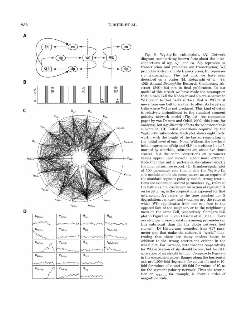
Fig. 6. Wg-Slp-En sub-module. (A) Networkdiagram summarizing known facts about the inter-connections of wg, slp, and en. Slp represses entranscription and promotes wg transcription; Wgpromotes both en and slp transcription; En repressesslp transcription. The last link we have seendescribed on a poster (M. Kobayashi et al., ’98,40th Annual Drosophila Research Conference, Ab-stract 184C) but not in final publication. In ourmodel of this circuit we have made the assumptionthat in each Cell the Nodes en and slp are sensitive toWG bound to that Cell’s surface; that is, WG mustmove from one Cell to another to affect its targets inCells where WG is not produced. This kind of detailis relatively insignificant to the standard segmentpolarity network model (Fig. 1A; see companionpaper by von Dassow and Odell, 2002, this issue, foranalysis), but significantly affects the behavior of thissub-circuit. (B) Initial conditions required by theWg-Slp-En sub-module. Each plot shows eight Cells’worth, with the height of the bar corresponding tothe initial level of each Node. Without the low-levelinitial expression of slp and SLP in positions 1 and 5,marked by asterisks, solutions are about five timesscarcer, but the same restrictions on parametervalues appear (not shown), albeit more extreme.Note that this initial pattern is also almost exactlythe final pattern we expect. (C) Drunken-spider plotof 100 parameter sets that enable the Wg-Slp-Ensub-module to hold the same pattern as we require ofthe standard segment polarity model; strong restric-tions are evident on several parameters. kXy refers tothe half-maximal coefficient for action of regulator Xon target y; nXy is the cooperativity exponent for thatinteraction; HX refers to the time constant for Xdegradation; rMxferWG and rLMxferWG are the rates atwhich WG equilibrates from one cell face to theapposed face of the neighbor, or to the neighboringfaces on the same Cell, respectively. Compare thisplot to Figure 2a in von Dassow et al. (2000). Thereare stronger cross-correlations among parameters inthis subcircuit than for the whole network (notshown). (D) Histograms compiled from 617 para-meter sets that make the subcircuit ‘‘work,’’ illus-trating that there are many modest biases inaddition to the strong restrictions evident in thewheel plot. For instance, note that the cooperativityfor WG activation of slp should be low, but for SLPactivation of wg should be high. Compare to Figure 6in the companion paper. Ranges along the horizontalaxis are 1,000-fold (log scale) for values of k and r, 10-fold for values of n, and 100-fold for values of H, asfor the segment polarity network. Thus the restric-tion on kSLPwg, for example, is about 1 order ofmagnitude wide.

E. MEIR ET AL.232

become critical adjuncts to lab-bench molecularbiology, just as they have become for various fieldsfrom enzymology to ecology. Yet most biologists donot presently receive or seek the mathematicaland computer science training they would need todevelop such tools on their own or even to usegeneral-purpose mathematical software. A pro-gram like Ingeneue can build mathematicallyrigorous models using a syntax that biologistswith brief training in differential equations canlearn easily. This biologist can then explore his orher favorite networks through the graphical inter-face and gain an intuitive understanding of itsdynamical behavior as a whole mechanism. Thiskind of computer-assisted synthesis, if madeaccessible to the scientists that actually confrontthe biological subject every day, will help us allunderstand gene network mechanics better.

We designed Ingeneue to facilitate its use as afairly general tool. Because the code is object-oriented and separated into distinct pieces that donot rely explicitly upon each other’s details,Ingeneue can be easily extended to add features,methods, and facilities. This is particularly evidentin the Affectors, where it takes a trivial amount ofcode to add a new formula. The same thing is truefor pattern-matching algorithms, search strate-gies, initial conditions, and the graphical interface.In addition to ease of modification, the program’sstructure has made it easy for us to replacemathematical formulas with names (of Affectors,for instance), and in the future with graphicalsymbols, that can be combined together to makemodels. Ultimately this architecture will become agrammar and syntax for translating a diagram of agene network to a set of mathematical equationsand back again. Using this syntax we canconstruct new networks almost entirely from theexisting Affectors in relatively short times. Eventhose of us who have some mathematical trainingfind this tremendously helpful! Perhaps even moreimportant, the stereotyping of building blocksmakes it easier to compare one model to another;if two models have been built from the sameparts and analyzed the same way, the resultsshould be more readily comparable than if twodifferent artisans crafted them in their ownstyles. Just as helpful is Ingeneue’s ability toinstantiate a network over a field of cells, correctlyhooking up exchanges of all the transmembranecomponents and eliminating many of the smallmistakes that would inevitably creep in whentrying to keep track of so many equations byhand.

We do not think of Ingeneue as the ultimate inpattern formation simulators. Ingeneue is stillvery much a work in progress, and seriousconceptual and technical weaknesses remain.One deficiency is Ingeneue’s current inability todeal with morphogenesis or cell movement. Inmany cases, developmentally interesting patternsare formed at the same time that cells are dividing,moving around, and changing neighbors. Thesemovements may be intimately coupled to thepattern formation process. Furthermore, Inge-neue assumes cells to be well-stirred reactionbeakers (although we impose compartmentaliza-tion, e.g., separating cell faces), an approximationthat no one even remotely believes. Indeed, almostevery well-understood developmental mechanismincludes some fascinating and functionally impor-tant instance in which the structure of cells playsa crucial role: apical–basal sorting of receptors andligands; the flexibility of stretches of chromatin;clustering of receptors; etc. Models of all kindsmust balance tractability with realism. In Inge-neue we have chosen a certain level of realismwhich may limit its usefulness but which allows usto use it to explore parameter space in a way that amore realistic modeling framework would pre-clude because of the computational burden.

Another weak spot in our approach is theproblem of recognizing patterns. Although we havea mechanism in place to build complex patternrecognizers from smaller pieces, pattern recognitionis a hard problem, and it is not clear whether ourmechanism will work in general without imposingan onerous coding and training burden on the user.Thus some uses of Ingeneue are still likely toinvolve clever custom programming, although thiswill hopefully decrease as the program matures. Nomatter what, we doubt very much that anycomputer recipe can, without extensive training,replace the intuition of the human biologist when itcomes to pattern recognition.

We have been using Ingeneue to address a widevariety of questions in developmental and evolu-tionary biology (von Dassow et al., 2000; Meiret al., 2002; Odell et al., unpublished observations;von Dassow and Odell, 2002). These includesimply asking, how complete is our currentunderstanding of a gene network? Given theknown facts, is the proposed mechanism plausi-ble? And, how do the different components of anetwork contribute to its behavior? We have alsoused Ingeneue to ask how important particularclasses of interactions are to the functioning of anetwork, and to explore how the structure of a


network affects its function. The examples aboveillustrate some of these results. Most of all, we feelthat through model-building we can translatewhat the community of developmental biologistsknows about developmental mechanics into thetheoretical framework of evolutionary biology. Forexample, our model of the segment polarity net-work unexpectedly yielded a putative example ofthe mechanistic origins of canalization. We hopethat these beginnings and the free availability ofthis program will inspire other biologists to trysimilar explorations.

ACKNOWLEDGMENTS

Thanks to Dara Lehman for comments on earlydrafts. Funding for the development of Ingeneueand for other work mentioned here came from theNational Science Foundation (MCB-9732702,MCB-9817081, MCB-0090835). Much of the workdescribed here was done at Friday Harbor La-boratories, and we thank Dennis Willows and theFHL staff for space and support. Appendix B waspreviously published as part of GvD’s doctoralthesis (University of Washington Department ofZoology, 2000). We dedicate this paper to thememory of Dr. DeLill Nasser, program director ingenetics at NSF. DeLill encouraged us even in theearly exploratory stages of this work, before therewas any buzz about bio-informatics, when evenwe ourselves weren’t sure this project wouldamount to much. We are deeply grateful for heropen-minded vision.

LITERATURE CITED

Arnosti DN, Barolo S, Levine M, Small S. 1996. The eve stripe2 enhancer employs multiple modes of transcriptionalsynergy. Development 122:205–214.

Aza-Blanc P, Ramirez-Weber FA, Laget MP, Schwartz C,Kornberg TB. 1997. Proteolysis that is inhibited by hedge-hog targets Cubitus interruptus protein to the nucleus andconverts it to a repressor. Cell 89:1043–1053.

Barkai N, Leibler S. 1997. Robustness in simple biochemicalnetworks. Nature 387:913–917.

Barkai N, Leibler S. 2000. Circadian clocks limited by noise.Nature 403:267–268.

Bhat KM, van Beers EH, Bhat P. 2000. Sloppy paired acts asthe downstream target of wingless in the Drosophila CNSand interaction between sloppy paired and gooseberryinhibits sloppy paired during neurogenesis. Development127:655–665.

Bray D, Levin MD, Morton-Firth CJ. 1998. Receptor cluster-ing as a cellular mechanism to control sensitivity. Nature393:85–88.

Burden RL, Faires JD, Reynolds AC. 1978. Numericalanalysis. Boston: Prindle, Weber and Schmidt.

Burke R, Nellen D, Bellotto M, Hafen E, Senti KA, DicksonBJ, Basler K. 1999. Dispatched, a novel sterol-sensingdomain protein dedicated to the release of cholesterol-modified hedgehog from signaling cells. Cell 99:803–815.

Cadigan KM, Grossniklaus U, Gehring WJ. 1994a. Functionalredundancy: the respective roles of the two sloppy pairedgenes in Drosophila segmentation. Proc Natl Acad Sci U S A91:6324–6328.

Cadigan KM, Grossniklaus U, Gehring WJ. 1994b. Localizedexpression of sloppy paired protein maintains the polarity ofDrosophila parasegments. Genes Dev 8:899–913.

Cash JR, Karp AH. 1990. A variable order Runge–Kuttamethod for initial value problems with rapidly varyingright-hand sides. ACM Trans Math Software 16:201–222.

Dierick HA, Bejsovec A. 1998. Functional analysis of Winglessreveals a link between intercellular ligand transport anddorsal-cell-specific signaling. Development 125:4729–4738.

Driever W. 1993. Maternal control of anterior development inthe Drosophila embryo. In: Bate M, Martinez-Arias A,editors. The development of Drosophila melanogaster. Plain-view, NY: Cold Spring Harbor Laboratory Press. p 301–324.

Driever W, Thoma G, Nusslein-Volhard C. 1989. Determina-tion of spatial domains of zygotic gene expression in theDrosophila embryo by the affinity of binding sites for thebicoid morphogen. Nature 340:363–367.

Edgar BA, Weir MP, Schubiger G, Kornberg T. 1986.Repression and turnover pattern fushi tarazu RNA in theearly Drosophila embryo. Cell 47:747–754.

Edgar BA, Odell GM, Schubiger G. 1989. A genetic switch,based on negative regulation, sharpens stripes in Drosophilaembryos. Dev Genet 10:124–142.

Gibson G. 1996. Epistasis and pleiotropy as natural propertiesof transcriptional regulation. Theor Popul Biol 49:58–89.

Gibson G, Wagner G. 2000. Canalization in evolutionarygenetics: a stabilizing theory? BioEssays 22:372–380.

Goodrich LV, Johnson RL, Milenkovic L, McMahon JA, ScottMP. 1996. Conservation of the hedgehog/patched signalingpathway from flies to mice: induction of a mouse patchedgene by Hedgehog. Genes Dev 10:301–312.

Grossniklaus U, Pearson RK, Gehring WJ. 1992. TheDrosophila sloppy paired locus encodes two proteinsinvolved in segmentation that show homology to mamma-lian transcription factors. Genes Dev 6:1030–1051.

Gurdon JB, Harger P, Mitchell A, Lemaire P. 1994. Activinsignalling and response to a morphogen gradient. Nature371:487–492.

Johnson LW, Reiss RD. 1982. Numerical analysis. Reading,MA: Addison-Wesley.

Kauffman SA. 1993. The origins of order: self-organizationand selection in evolution. New York: Oxford UniversityPress. xviii, 709 pp.

La Rosee A, Hader T, Taubert H, Rivera-Pomar R, Jackle H.1997. Mechanism and Bicoid-dependent control of hairystripe 7 expression in the posterior region of the Drosophilaembryo. EMBO J 16:4403–4411.

Laub MT, Loomis WF. 1998. A molecular network thatproduces spontaneous oscillations in excitable cells ofDictyostelium. Mol Biol Cell 9:3521–3532.

Lee HH, Frasch M. 2000. Wingless effects mesoderm pattern-ing and ectoderm segmentation events via induction of itsdownstream target sloppy paired. Development 127:5497–5508.

Marigo V, Scott MP, Johnson RL, Goodrich LV, Tabin CJ.1996. Conservation in hedgehog signaling: induction of a

E. MEIR ET AL.234

chicken patched homolog by Sonic hedgehog in the devel-oping limb. Development 122:1225–1233.

McAdams HH, Shapiro L. 1995. Circuit simulation of geneticnetworks. Science 269:650–656.

Meir E, von Dassow G, Munro E, Odell GM. 2002. Robustness,flexibility, and the role of lateral inhibition in the neuro-genic network. Curr Biol 12:778–786.

Moline MM, Southern C, Bejsovec A. 1999. Directionality ofwingless protein transport influences epidermal patterningin the Drosophila embryo. Development 126:4375–4384.

Murray JD. 1993. Mathematical biology. Berlin: Springer-Verlag. xiv, 767 pp.

Nellen D, Burke R, Struhl G, Basler K. 1996. Direct and long-range action of a DPP morphogen gradient. Cell 85:357–368.

Pai LM, Orsulic S, Bejsovec A, Peifer M. 1997. Negativeregulation of Armadillo, a Wingless effector in Drosophila.Development 124:2255–2266.

Pfeiffer S, Vincent JP. 1999. Signalling at a distance:transport of Wingless in the embryonic epidermis ofDrosophila. Semin Cell Dev Biol 10:303–309.

Porter JA, Ekker SC, Park WJ, von Kessler DP, Young KE,Chen CH, Ma Y, Woods AS, Cotter RJ, Koonin EV, BeachyPA. 1996. Hedgehog patterning activity: role of a lipophilicmodification mediated by the carboxy-terminal autoproces-sing domain. Cell 86:21–34.

Press WH. 1992. Numerical recipes in C: the art of scientificcomputing. New York: Cambridge University Press. xxvi,994 pp.

Ptashne M. 1992. A genetic switch: phage l and higherorganisms. Cambridge, MA: Cell Press, Blackwell ScientificPublications. ix, 192 pp.

Reinitz J, Sharp DH. 1995. Mechanism of eve stripe forma-tion. Mech Dev 49:133–158.

Slack JMW. 1983. From egg to embryo: determinative eventsin early development. New York: Cambridge UniversityPress. 241 pp.

Struhl G, Struhl K, Macdonald PM. 1989. The gradientmorphogen bicoid is a concentration-dependent transcrip-tional activator. Cell 57:1259–1273.

Thieffry D, Huerta AM, Perez-Rueda E, Collado-Vides J. 1998.From specific gene regulation to genomic networks: a globalanalysis of transcriptional regulation in Escherichia coli.BioEssays 20:433–440.

Tyson JJ, Novak B, Odell GM, Chen K, Thron CD. 1996.Chemical kinetic theory: understanding cell-cycle regula-tion. Trends Biochem Sci 21:89–96.

von Dassow G, Meir E, Munro EM, Odell GM. 2000. Thesegment polarity network is a robust developmental module.Nature 406:188–192.

von Dassow G, Odell GM. 2002. Design and constraints of theDrosophila segment polarity module: robust spatial pattern-ing emerges from intertwined cell state switches. J Exp Zool(Mol Dev Evol) 294:179–213.

Weir MP, Edgar BA, Kornberg T, Schubiger G. 1988. Spatialregulation of engrailed expression in the Drosophilaembryo. Genes Dev 2:1194–1203.

APPENDIX A: MATHEMATIZING GENEREGULATORY INTERACTIONS

We outline a general approach for convertingempirical descriptions of network interactions intothe mathematical formulae that Affector objectsencapsulate. We focus on transcription as anexample because it is a form of network interac-tion that involves a wide range of regulatoryphenomena, but the methods we describe can bereadily applied to the other types of Affectors.

General form of transcriptionalAffector equations

A transcriptional Affector determines the tran-scription rate for a Node as a function of allregulatory influences impinging on that Node(each Node has at most one primary synthesisAffector). In dimensional terms, the rate equationfor a transcriptional Affector has the general form

d½x�dt

¼ Tmax�xFð½R1�; ½R2�; . . . ; ½RN�Þ: ðA1Þ

Tmax is the maximal possible transcription rate forany gene, determined by the enzymology of RNApolymerase, and �x is an efficiency characteristic ofgene x, reflecting how good a template x is.F : <N ! ½0; 1�, a function of the regulator con-centrations ð½R1�; ½R2�; . . . ; ½RN�Þ, determines at

what fraction of full efficiency x is transcribed.By definition, values of F must lie between 0 and 1inclusive. Building an Affector formula for a givenregulation mechanism amounts to determining anappropriate functional form for F, and parame-trizing it.

A simple example: transcriptionalactivation

We start with a very simple example whichforms the basis for all the more complicatedregulatory schemes described below. Consider asingle regulatory factor A, which activates tran-scription of gene x. For mathematical clarity, wefocus attention on one copy of x (unless transcrip-tional regulators are present in very low numbers,the overall transcription rate is simply twice therate from one copy). Without any significant loss ofgenerality, we can think of the underlying me-chanism as involving two steps (Fig. A1): in thefirst step, A interacts with a specific DNAsequence in a concentration-dependent way toform an ‘‘active complex’’ An. For example, Amight bind directly to DNA, or bind as part of alarger complex involving other molecules, orcatalyze the formation of a complex which binds toDNA without itself doing so. In the second step,the active complex An interacts with a proximalpromoter region to boost the rate at which new


transcripts are initiated. Again, there are manypossible ways this could occur: An could modify thelocal structure of chromatin to allow greater accessto other transcription factors, or associate moredirectly with proximal transcriptional machinery orthe proximal promoter to recruit one to the other,etc.

With this general mechanism in mind, we canwrite FðAÞ as

FðAÞ ¼ �A�ðAÞ; ðA2Þwhere �ðAÞ is the fraction of time that the activecomplex An exists as a function of A’s concentra-tion, and �A is the efficiency with which An booststranscription of x. Alternatively, we can think ofF Að Þ as representing the probability that x istranscriptionally active at a given point in time,where transcriptionally active means that x istranscribed at its maximum rate Tmax�x. In thiscase, �ðAÞ represents the probability that anactive complex exists at a given point in time,and �A represents the conditional probability thatx is transcriptionally active, given that an activecomplex exists, or simply the probability that An

activates x. This probabalistic interpretation turnsout to be very useful in building representations ofmore complex forms of regulation, as we willreturn to below.

In the case of simple activation, and in theabsence of any detailed knowledge about how Ainteracts with gene x, we use the simple genericform for �ðAÞ:

�ðAÞ ¼½A�KA

� ��A1 þ ½A�

KA

� ��A ¼ ½A��AK�A

A þ ½A��A� �

; ðA3Þ

where KA is the value at which �ðAÞ ¼ 0:5 and �Ais the degree of cooperativity. As discussed in thetext, we can think of �ðAÞ as a measurable dose–response curve, expressing in the most generalterms what must be the case for an interactionbetween A and x: that the magnitude of theinteraction must increase and then saturate withincreasing concentrations of A, that it does somore or less steeply, and that A has a maximaleffectiveness as an activator of x.

To represent more complicated forms of tran-scriptional regulation involving multiple regula-tors, we replace �ðAÞ and A with more complicatedexpressions, which we must deduce from what weknow about those additional regulators and theirinteractions. We have taken two general ap-proaches to doing so. The first generalizes fromsimple kinetics to produce replacements for �ðAÞ.The second represents interactions as logicalconditions and uses simple probability theory.

Deducing regulatory forms fromsteady-state kinetics

Many transcriptional regulators are known tointeract either before or during complex forma-tion. For example, different activators bind toDNA as heterodimers, or otherwise assembleactive complexes around the same or nearbyDNA sequences. Many inhibitors act by competingwith an activator for its binding site or by bindingto and titrating away an activator before it binds.In these cases, we can deduce suitable regulatoryforms by 1) writing down the simplest kineticscheme that summarizes (or caricatures) what weknow about the binding interactions amongregulators and DNA sequences; 2) solving theresulting kinetic rate equations to find the steadystate concentration of whatever complex we areinterested in; 3) where necessary or convenient,approximating the resulting steady state expres-sion with an appropriate simpler form; and 4)generalizing the resulting form in an appropriateway to allow for cooperative effects. We willillustrate this approach with several examples.

Example 1: A single activator binds atarget DNA sequence

Consider first the simple kinetic scheme inwhich activator A binds to a specific sequence Swithin the regulatory region of gene x to form thebound complex AS (Fig. A2A):

Aþ S,kþ

k�AS: ðA4Þ

Fig. A1. Schematic view of transcriptional regulation as atwo-step process. In step 1, regulator A forms an activecomplex An around sequence S in a concentration-dependentmanner. The fraction of bound complex is given by C(A). Instep 2, the active complex An regulates the rate at whichtranscription is initiated at the proximal promoter withefficiency 0raAr1 (see text for details).

E. MEIR ET AL.236

Fig. A2. Deducing pseudo-kinetic representations of reg-ulatory interactions from kinetic interaction diagrams. Leftcolumn shows interaction diagrams. Right column shows thealgebraic forms we deduce from those diagrams by assumingall binding reactions are at steady state, making use of simpleapproximations where necessary, and generalizing to includecooperative effects. S indicates a specific DNA sequence. A andB represent transcriptional activators, and I represents atranscriptional inhibitor. Arrows indicate reversible reactions(only the forward half of each reaction is shown for clarity).Plus sign (or minus sign) within a circle indicates a positive (ornegative) regulation of the indicated reaction. (A) An activatorbinds a target DNA sequence (present at two copies per cell) toform an active complex. The fraction of bound complex is givenby the generalized function C(A) shown to the right. (B) Twomolecules (each present at arbitrary concentrations) bind toform a dimer complex. To the right are the exact concentrationof dimer, and the approximate form O(A,B) generalized to

arbitrary cooperativity. (C) An inhibitor I binds to and titratesaway an activator A before it binds to a target DNA sequence Sto form an active complex. The fraction of active complex isgiven by the same function C shown in (A), but in this case,the amount of A available to bind its target is the total amountof A minus the amount of bound activator–inhibitor complexO(A,I) as shown to the right. (D) An inhibitor acts tocompetitively exclude A from binding to its target sequenceS. Here we show I binding to S itself, but it could also bind toan adjacent sequence. To the right is the generalized steady-state form, obtained by assuming that A and I bind withentirely independent affinities and cooperativities. (E) Reg-ulator B boosts A’s efficacy as a transcriptional activator byconverting it from a low-affinity form (A) to a high-affinityform (AP). In this case, several successive approximations arerequired to obtain the simple form shown to the right. (F)Similar to E, but in this case I converts A from a high-affinityto low-affinity form.


The resulting equations are:

d½AS�dt

¼ kþ½A�½S� � k�½AS�; ½AS� þ ½S� ¼ 1; ðA5Þ

where the second equation expresses the stoichio-metric fact that there is a single sequence whichmust be in either a bound or unbound state. Wethen set d½AS�=dt ¼ 0 and solve for the steady-

state fraction of bound complex AS to obtain

½AS� ¼½A�K

1 þ ½A�K

¼ ½A�K þ ½A� ; ðA6Þ

where K ¼ k�=kþ becomes the half-maximal acti-vation coefficient. To obtain the generic form� ½A�ð Þ, we simply apply a cooperativity exponent�A to each appearance of [A] and K in Eq. (A6).

Example 2: Protein dimerization and itsgeneralization

Now consider a similar reaction in which A andB are two proteins that bind to form the hetero-dimer AB (Fig. A2B):

Aþ B,kþ

k�AB: ðA7Þ

Unlike Example 1 where [A] changes negligibly asa consequence of the reaction, in general, both [A]and [B] might change as a consequence ofdimerization, and indeed we may often be inter-ested in the fraction remaining unbound. Thus weneed to be more explicit in the associated kineticequations:

d½Afree�dt

¼ k� � ½AB� � kþ � ½Afree�½Bfree�;

d½Bfree�dt

¼ k� � ½AB� � kþ � ½Afree�½Bfree�;

d½AB�dt

¼ kþ � ½Afree�½Bfree� � k� � ½AB�;

½A� ¼ ½Afree� þ ½AB�;½B� ¼ ½Bfree� þ ½AB�:

ðA8Þ

Here [A] and [B] represent the total concentra-tions of reactants, [Afree] and [Bfree] represent theconcentrations of free (unbound) reactants, and[AB] is the total concentration of bound complex.Solving Eq. (A8) at steady state (or just using themass action law’s formula for the equilibriumcondition, Keq ¼ ½AB�=½Afree�½Bfree�), substituting for[Afree] and [Bfree] from the mass balance equa-tions, and using K ¼ k�=kþ ¼ 1=Keq we obtain thequadratic equation

½A� � ½AB�ð Þ ½B� � ½AB�ð ÞK

� ½AB� ¼ 0 ðA9Þ

with a single positive root given by

½AB� ¼

K þ ½A� þ ½B�ð Þ �ffiffiffiffiffiffiffiffiffiffiffiffiffiffiffiffiffiffiffiffiffiffiffiffiffiffiffiffiffiffiffiffiffiffiffiffiffiffiffiffiffiffiffiffiffiffiffiffiffiffiffiffiffiffiffiffiK þ ½A� þ ½B�ð Þ2�4 � ½A�½B�

q2

:

ðA10Þ

Fig. A3. Deducing regulatory forms using simple probabil-ities. (A) Two activators, A1 and A2, bind to separate enhancerelements, S1 and S2, and independently activate transcriptionfrom the proximal promotor with probabilities (efficiencies) a1

and a2. (B) A single inhibitor I binds to its enhancer elementSI and globally inhibits transcription as activated by either A1

or A2 with probability (efficiency) aI. (C) Inhibitor I binds toenhancer element SI and inhibits A1’s activation of transcrip-tion with probability (efficiency) aI but has no effect ontranscription as activated by A2.

E. MEIR ET AL.238

Equation (A10) is a perfectly good way to estimatethe steady state of a dimerization reaction exactly,but it is non-intuitive and difficult to generalize(i.e., to add cooperativity). To this end, weintroduce a simpler function:

½AB� ¼ �ð½A�; ½B�;KABÞ ¼½A�½B�KAB

1 þ ½A�KAB

þ ½B�KAB

¼ ½A�½B�KAB þ ½A� þ ½B� : ðA11aÞ

If we want the fraction of [A] (or [B]) unbound weuse the relation ½Afree� ¼ ½A� � ½AB�:½Afree� ¼� ½A�; ½B�; KABð Þ ¼ ½A� � ½A�½B�

KAB þ ½A� þ ½B�

¼½A� 1 � ½B�KAB þ ½A� þ ½B�

� �: ðA11bÞ

Equation (A11) has the same qualitative proper-ties as Eq. (A10): it is symmetric to exchangeof A and B; for fixed [A], it saturates to the value of[A] with increasing [B] (and vice versa); itincreases without bound as both [A] and [B]increase. It is a good approximation to Eq. (A10)in the sense that, for any value of K in Eq. (A10),we can find a value of KAB in Eq. (A11) suchthat the difference between Eqs. (A10) and (A11)is small for all values of [A] and [B] (we formalizethis notion below). Finally, we can generalizeEq. (A11) to add a ‘‘cooperativity’’ effect6

as follows:½AB� ¼ � ½A�; ½B�;KAB; �ABð Þ

¼ ½A� ½B��ABK�AB

AB þ ½A��AB þ ½B��AB� �

;

½Afree� ¼ � ½A�; ½B�;KAB; �ABð Þ

¼ ½A� 1 � ½B��ABK�AB

AB þ ½A��AB þ ½B��AB� �

:

ðA12Þ

Example 3: A form of competitiveinhibition

Here is how we would use the same approachas in Example 1 to model competitive inhibition in

which activator A and inhibitor I bind to thesame sequence S (Fig. A2D). In this case, thekinetic scheme is

Aþ S,kþA

k�A

AS;

I þ S,kþI

k�I

IS:

ðA13Þ

The resulting equations are

d½AS�dt

¼ kþA ½A�½S� � k�A ½AS�;

d½IS�dt

¼ kþI ½I�½S� � k�I ½IS�;

½AS� þ ½IS� þ ½S� ¼ 1;

ðA14Þ

and solving them at steady state yields

½AS� ¼ F Að Þ 1 � F Ið Þð Þ1 � F Að ÞF Ið Þ ; ðA15Þ

where

F Að Þ ¼½A�KA

1 þ ½A�KA

; KA ¼ k�AkþA

; ðA16Þ

as for Example 1 above. We can generalize thisform exactly as described for Example 1 above byreplacing the functions F(A) and F(I) with thegeneric forms � Að Þ and � Ið Þ to obtain:

½AS� ¼� Að Þ 1 � � Ið Þð Þ1 � � Að Þ� Ið Þ

¼½A��A 1 � ½I��I

K�IIþ½I��I

� �

K�AA þ ½A��A 1 � ½I��I

K�IIþ½I��I

� �0BB@

1CCA

¼AKA

� ��A1 þ A

KA

� ��Aþ I

KI

� ��I0B@

1CA: ðA17Þ

However, Eq. (A15) could be generalized differ-ently, such that I affects the concentration of Abefore application of the exponent in �. Thiscorresponds to a choice that is simple to explainmathematically but rather complicated to unwindmechanistically: does the inhibitor affect theeffective concentration of A directly, or does itaffect A activity ‘‘after’’ A has assembled intowhatever bound complex confers the cooperativityexponent? Figure A5B and C contrast these twochoices. A fourth choice, not plotted in Fig. A5but diagrammed as Fig. A2C, would multiply [A]

6This introduces an asymmetry between A and B. However, this isrealistic. Cooperative binding phenomena usually involve a singlemacromolecule (say, a single molecule of A, even if A is in fact a proteincomplex) that binds several ligands. Examples include hemoglobinbinding to oxygen, and IPTG binding to the lac repressor; bothmacromolecules are tetramers. A typical treatment of such a caseassumes the ligand is present in vast excess, and thus results inEq. (A3). However, if the ligand could be present at similarconcentration to its partner, or if what we know is the total ligandconcentration rather than the concentration of unbound ligand, thenEq. (A3) is inadequate and potentially misleading. The rigoroustreatment of such a case is complicated, and we emphasize that Eqs.(A11) and (A12) are only offered as convenient approximations whosequalitative behavior matches our expectations of the behavior of such asystem.


by � ½A�; ½I�; KIA; �IAð Þ prior to the computation of� ½Afree�; KA; �Að Þ; this approximates a mechanismin which the inhibitor titrates away free A beforeA binds its target sequence.

Figure A2 shows some of the other forms onecan readily deduce to describe different types ofregulatory interaction. The forms fall into twogeneral classes. Forms in the first class (Fig. A2Aand A2C–F) are dimensionless and have valuesthat lie strictly within the interval [0,1]. Each ofthese forms represents the fraction of time thatsome active complex exists and therefore ‘‘fits’’into the general form of F(A) given as Eq. (A2)above. Forms in the second class (Fig. A2B) havedimensions of concentration and therefore fit asarguments to the general form F(A). All reduceto the appropriate simpler forms when one ormore of the regulators are absent.

We want to stress that these forms are notintended to be literal kinetic representations ofsome detailed regulatory mechanism, which willusually involve, in reality, a great deal morealgebraic gore. If we knew all of the details ofsuch a mechanism, then we could deduce such aliteral representation and incorporate it into theframework described here. But even if we could,there would be little advantage in using a detailedrepresentation of one interaction within a networkif we are only using cruder approximations some-where else. However, it is instructive to think ofthe equations we deduce as approximations to theliteral kinetic forms and then ask whether theyare ‘‘good’’ approximations.

To do so, we must define what we mean by‘‘good’’. Suppose FapproxðR1;R2;p1; p2; p3Þ is anapproximate form deduced as above for tworegulators R1 and R2 of gene x, and parameterizedby p1, p2, and p3. Suppose further that we actuallyknew all of the underlying molecular playersinvolved in mediating interactions of R1 and R2

with x. Then we could write down a complex set ofkinetic equations expressing these interactionsand solve them at steady state to deduce an‘‘exact’’ (not really) function FexactðR1;R2;C1; :::;CN; k1; :::kMÞ where the C’s and k’s are theconcentrations7 of those underlying players andkinetic parameters governing their interactions.The set of all possible values for the parametersðC1; . . . ;CN; k1; . . . ; kMÞ determines a range ofshapes of Fexact as a function of R1 and R2. We

say that FapproxðR1;R2Þ is a good approximation ofFexactðR1;R2Þ if it manifests a quantitativelysimilar set of shapes when we vary the parametersðp1; p2; p3Þ. Another way to say this is thatFapproxðR1;R2Þ is a good approximation ofFexactðR1;R2Þ if for any choice of parameters forFexact ðC0

1; . . . ;C0N; k

01; . . . ; k

0NÞ, there exists a choice

of values ðp01; p02; p03Þ, such that FexactðR1;R2;C0

1; . . . ;C0N;k

01; . . . ;k

0NÞ and Fapproxðp01; p02; p03Þ have

similar shapes.Of course, we cannot compare our approximate

representations to the literal ones because we donot know what the literal ones are. But we cancompare two different approximate schemes thatrepresent the same regulatory scheme at differentlevels of resolution (where one might includeadditional intermediates or auxiliary proteinspresent at constant concentrations). Where wehave done so, we find that the simpler schemes aresurprisingly good at approximating the morecomplicated ones, good enough that we can findno reason to use the more complicated ones in ournetwork models.

We can use this same notion to comparedifferent ways of representing the same set ofempirically observed regulatory interactions. Forexample, we deduced many of the regulatoryforms we used in our early models by intuition,seeking formulae whose properties expressedadequately what we took to be the basic empiricalfacts. In many cases, we find that different formsare equivalently good representations of a parti-cular regulatory interaction in the sense that eachapproximates the others as defined above (seeFigs. A4 and A5). In this case, we are free to applyother criteria to choose the ‘‘best’’ one, e.g., whichis most easily parametrized, or makes the mostbiological sense, or combines most easily withother forms.

We emphasize that the important distinctionbetween these different formula options is thedistinction between their graphs (Figs. A4 and A5)and the qualitative properties thereof. For exam-ple, compare the shapes in Fig. A5A,D,G,J withthe shapes in Fig. A5C,F,I,L; in Fig. A5D, aparticular concentration of the inhibitor (movingto the left) squelches activation by a certainfraction no matter what the level of activator; inFig. A5F, this is not so. The difference is that inthe formula governing the left column the in-hibitor regulates the maximal activity level,whereas in the right column the inhibitor reg-ulates how much activator is required to achievethat level, and in the middle column inhibitor

7We assume that the concentrations of the underlying players areconstant on the timescale of interest. Otherwise, we would have toinclude them in our pseudo-kinetic representation.

E. MEIR ET AL.240

regulates availability of the acivator (that is,inhibitor modulates Tmax versus k versus [A]).Other scenarios (especially mixes of these) arebiologically plausible. Often the model-makersimply will not have the information to choose,and the fact is that in certain circumstances, someshapes work, and others don’t (see example of wgautoregulation in the companion paper by vonDassow and Odell, ’02, this issue).

Using logical descriptions andprobabilities to deduce regulatory

forms

As mentioned above, we can think of bindingfractions and interaction efficiencies in probabil-istic terms. Doing so provides a powerful way todeduce representations for more complicatedtypes of regulation. To see how, we must introducemore notation. First, we must define the condi-tions whose probabilities we would like to repre-sent. Let X be a gene and R be one of its regulators,

and let

�xx be the condition : ‘‘x is transcriptionally active00:

R� be the condition : ‘‘An active complex;

representing the interaction

between R and x; exists00:

R� ! x be the condition : ‘‘The active complex

regulates x00:

More generally, we use A ! B to mean ‘‘A has itscharacteristic effect on B,’’ and we use thisnotation wherever A and B are such that thecondition A ! B makes sense. Finally, we let P(C)be the probability that condition C holds at a givenpoint in time. For convenience we will use &&, 3,and ! interchangeably with logical AND, OR, andnegation, respectively. Returning to the simplecase of a single activator A and gene x, theprobability that x is transcriptionally active isthe probability that A activates x, which is the

Fig. A4. Formulas for transcriptional control by twoactivators. The differential equation at the top of the figureis typical for mRNAs: the concentration of x increases at a rateproportional to some non-linear function F of variousregulators, in this case two activators (A and B), and decreasesin proportion to the concentration of x. (A–D) Various forms off([A],[B]) with accompanying graphs. All graphs use theparameter values shown at the top, and plot normalizedvalues of [A] and [B] from 0.0 to 2.0. The simple formula in (A)has the advantage of reducing to a single Hill function in theabsence of either activator. It corresponds to the assumptionthat A and B bind the same site with different affinities andcooperativities, that each forms an active complex at that sitewhich activates transcription with maximal efficiency a¼1. Inother words, it’s what one obtains from computing the boundfraction of A in the presence of competitor B (Eq. (A17),rightmost coequal form) and adding it to the bound fraction ofB in the presence of competitor A. However, using thisformula both activators reach the same saturating level, andthe formula expresses neither additive nor synergistic effects,thus we have not much used it in practice. (B) is an alternativewhich, through the weights a and b, allows one to adjust therelative ability of each activator to saturate the targetpromoter, and causes the activators to have an additive, butsaturating, effect on transcription rate. However, among otheroddities, this formula does not reduce to the simple single-activator case in the absence of the other, and furthermore,the weight parameters change the meaning of the half-maximal coefficients kAx and kBx. Nevertheless this formulamay be a reasonable approximation to certain two-stepenhancer-binding phenomena, and we have used it in variousforms of the segment polarity network model (however, seethe companion paper by von Dassow and Odell, ’02, this issue).(C) is an improvement over (B) that, as described in the

Appendix text, multiplies the probabilities that either activa-tor will not be bound and then takes the complement of thisquantity to determine the overall transcriptional activity. Thisis the same as Eq. (A22) but with a slight change in how theweights are treated (w is the ratio aA1/aA2; since in this formulaone term must be able to effect a maximal response, it makessense to normalize all weights to the largest of them). FormulaC/Eq. (A22) does reduce to the simple case, does preserve themeaning of the half-maximal coefficients, allows for weightingand easy incorporation of inhibitors, and furthermore, readilylends itself to modularization in software such that one canstring together an arbitrary number of regulators into a singleadditive term. We prefer this form for additive activation. Drepresents another possibility for two activators that hasmany of the virtues of C but with different operation of theweights. E and F represent synergistic, rather than additive,activators. In E, one activator, B, has no effect in the absenceof the other, A, and on the other hand, A by itself is only a pooractivator, but both together fully saturate the promoter. In Fthe second activator, B, functions to lower the half-maximalconcentration of A, or in other words it makes A more potentbut has no effect itself, but nevertheless A can still achieve fullpromoter saturation in the absence of the cofactor. E suggestsan equivalent scheme in which B catalyzes the transformationof A (by phosphorylation or cleavage or what have you) from alow-affinity form to a high-affinity form. The same exactscheme could make B an inhibitor (if it promoted formation ofthe low-affinity form), as shown in F). These six formulasdoubtless do not cover all possibilities, but it is apparent thatthe choice of B, C, or D leaves one with qualitatively similardose-response behaviors, even though they may representdifferent kinetic mechanisms and may affect the parameter-ization of the model differently. The same cannot be said of Eand F, however.

3

E. MEIR ET AL.242

Fig. A5. Formulas for transcriptional control by anactivator and inhibitor. All three formulas shown at the topare derived in the Appendix text; the individual graphs, whichplot normalized values of [A] and [I] from 0.0 to 2.0, representeach of the formulas with different choices of nAx and nIx, asshown to the left of each row. In all graphs kAx¼0.5, kIx¼0.8.For (A–I) nAx¼3, representing modest cooperativity for theactivator; A–C impose a non-cooperative inhibitor; D–F, amoderately cooperative inhibitor; G–I, a highly cooperativeinhibitor; and J–L combine a non-cooperative activator with amoderately cooperative inhibitor. A, D, G, and J showvariations of the formula derived in Eq. (A27), but withoutthe a’s. These parameters are left out; aA is redundant if there

is only a single activator, and aI merely prevents the inhibitorfrom fully squelching the activation term so we do not usuallyuse it. B, E, H, and K exhibit an alternate generalization ofEq. (A16), whereas C, F, I, and L exhibit the formula in Eq.(A17). The main conclusion we draw from this comparison isthat although the shape of the curve is broadly similar for eachformula, different choices dramatically affect how the para-meter ranges limit gene action. For example, the formula inthe middle column enables the strongest inhibition at highcooperativity, but at low cooperativity it resembles theformula in the right-most column (compare B and C andcompare K and L). Meanwhile, the formula in the right-mostcolumn is overall the ‘‘weakest’’ inhibition mechanism.


probability that A makes an active complex ANDthat active complex activates x. We can write

Pð�xxÞ ¼ PðA ! xÞ ¼ PððA�Þ&& ðA� ! xÞÞ¼ PðA�Þ � PðA� ! xÞ: ðA18Þ

The last equality above comes from the fact thatA� and A� ! x are independent conditions, andthus their joint probability is the product of theirindividual probabilities. This is simply Eq. (A3) indisguise, with Pð�xxÞ ¼ PðA ! xÞ ¼ FðAÞ,PðA�Þ ¼ �ðAÞ, and PðA� ! xÞ ¼ �A. To see howwe can extend this notation to describe newsituations, we must look at some examples.

Example 4: Independent activators

Suppose that we want to represent activation ofX by two independent activators A1 and A2, each ofwhich alone acts like A above (see Fig. A3A). Inthis case, the probability that x is transcriptionallyactive is the probability that A1 activates x OR A2

activates x:

FðA1;A2Þ ¼ Pð�xxÞ ¼ PðA1 ! xjjA2 ! xÞ: ðA19ÞUsing simple probability relations, we can quicklytransform the expression on the right-hand sideinto something useful;

PðA1 ! xjjA2 ! xÞ ¼Pð!ð!ðA1 ! xÞ&&!ðA2 ! xÞÞÞ ¼

1 � Pð!ðA1 ! xÞ&&!ðA2 ! xÞÞ;

ðA20Þwhere we have used the relations

PðAjjBÞ ¼ Pð!ð!AÞ&&ð!BÞÞ and Pð!AÞ ¼ 1 � PðAÞ:Since we assume A1 and A2 act independently, wecan reduce the joint probability on the right handside to the product of individual probabilites:

1 � Pð!ðA1 ! xÞ&&!ðA2 ! xÞÞ ¼1 � Pð!ðA1 ! xÞÞ � Pð!ðA2 ! xÞÞ ¼

1 � ð1 � PðA1 ! xÞÞ � ð1 � PðA2 ! xÞÞ: ðA21ÞFinally, putting Eqs. (A19), (A20), and (A21)together, and replacing the final probabilities inEq. (A21) from Eq. (A3), we obtain

FðA1;A2Þ ¼ 1 � ð1 � �A1�ðA1ÞÞ � ð1 � �A2

�ðA2ÞÞ:ðA22Þ

Note that this reduces to Eq. (A3) if either A1 orA2 is absent. Note also that we can immediatelygeneralize this expression to any number ofindependent activators:

FðA1; . . . ;ANÞ ¼ 1 �Y

i¼1�4N

1 � �Ai�ðAiÞ

� �: ðA23Þ

This is the virtue of this way of formulatingtranscriptional control Affectors: the programcode can interpret an arbitrary list of regulators,trivially building collections like Eq. (A23) asarrays of a few simple building blocks. This isthe basis for "meta-affectors" in the currentversion of Ingeneue.

Example 5: Inhibiting activation

Suppose now that factor A activates x and factorI inhibits this activation. We have already dealtwith the case in which I interferes with formationof the active complex An. Here we assume that Iacts downstream of complex formation. We canexpress the action of I the logical condition I !ðA� ! xÞ meaning ‘‘I prevents An from activatingx’’. In this case, the probability that A activates xis the joint probability that A makes an activecomplex AND that active complex is not inhibitedby I AND the uninhibited complex succeeds inactivating x:

FðA; IÞ ¼Pð�xxÞ ¼ PðA ! xÞ¼PðA�&& ð!I ! ðA� ! xÞÞ&& ðA� ! xÞÞ:

ðA24ÞIf the individual conditions are independent, thejoint probability is the product of their individualprobabilities, or

FðA; IÞ ¼PðA�Þ � Pð!I ! ðA� ! xÞÞ � PðA� ! xÞ¼ �A�ðAÞ � ð1 � PðI ! ðA� ! xÞÞÞ:

ðA25ÞFor generality, we assume that I binds to DNA toform an active complex In, which inhibits An’sactivation of x with some probability (or effi-ciency). We can then resolve the inhibition prob-ability exactly as we did above for the activator A:

PðI ! ðA� ! xÞÞ ¼ PðI�Þ � PðI� ! ðA� ! xÞÞ ¼ �I�ðIÞ;ðA26Þ

and we can put Eqs. (A25) and (A26) together toobtain

FðA; IÞ ¼ �A�ðAÞ � ð1 � �I�ðIÞÞ: ðA27ÞWe can easily extend the same approach torepresent a ‘‘global’’ inhibitor that interacts withthe basal transcription machinery to shut downactivation, regardless of activator concentration,by whatever mechanism. To do so, we simplyreplace the condition I ! ðA� ! xÞ with the moreglobal condition I ! ð�xxÞ. In this case, the prob-ability that x is transcriptionally active is simplythe probability that I does not inhibit the basal

E. MEIR ET AL.244

machinery AND the uninhibited x is active:

Pð�xxÞ ¼ Pð!I ! �xxÞ&&ð�xxUÞÞ¼ ð1 � �I�ðIÞÞ � Pð�xxUÞ: ðA28Þ

For example, if x is activated by N independentactivators, and globally inhibited by I (see Fig.A3B), then Pð�xxUÞ is given by Eq. (A23) above andwe have

FðI;A1; . . . ;ANÞ

¼ ð1 � �I � �ðIÞÞ 1 �Y

i¼1�4N

1 � �Ai� �ðAiÞ

� � !:

ðA29ÞBy this point, it should be apparent to the

reader without going through all the tediousprobabilities how we could begin to generalizethis process. To make an inhibitor target aparticular part of a transcription regulatorymechanism, we simply multiply the probabilityterm representing that part by the genericinhibitory term �ðIÞ ¼ ð1 � �I�ðIÞÞ. For example,if factors A1 and A2 activate x independently as inExample 4 and we want factor I selectively toinhibit A1 (see Fig. A3C), we multiply theefficiency �A1

in Eq. (A22) by �ðIÞ to obtain

FðI;A1;A2Þ ¼ 1 � ð1 � �A1��ðIÞ � �ðA1ÞÞ

� ð1 � �A2�ðA2ÞÞ: ðA30Þ

There is of course no reason why we could notchoose a slightly different mechanism for I, in which�ðIÞ nestles within �ðA1Þ somehow, as in Eq. (A17).

This trick is not limited to inhibitory influences.For example, we might know that factor B is‘‘required’’ for A to do its job and that it, too, mustbind to x to fulfill this requirement. If B isconstantly present, it becomes one of the manyshadowy co-conspirators that lurk beneath A ! A�

or A� ! x. However, if B is a dynamic part of ournetwork, we want to include that requirement.To do so, we could simply multiply the efficiencyterm for A, wherever it appears, by an activationterm for B:

�A ! �A�ðBÞ: ðA31ÞThe reader will no doubt think of other examples.

SUMMARY

The approach above has emerged from anongoing effort to encapsulate, in mathematicalequations, what physical intuition and empiricalfacts tell us about various forms of regulation.Given our current state of knowledge, these

formulations are necessarily approximate. Thereare many ways to invent equations that furnish areasonable representation of any particular formof regulation. Many of these are equivalent in thesense described above, namely, that one can beused to approximate the other with appropriatechoices of parameter (see Figs. A4 and A5). We donot claim that the approach described here willproduce the ‘‘right’’ equations in every case. But ithas a number of virtues that lend themselves tothe type of modeling we do. Chief among theseis that it provides a general way to ‘‘map’’biologists’ non-mathematical descriptions of net-work interactions to specific mathematical equa-tions whose parameters make intuitive biologicalsense and are at least in principle empiricallymeasurable. The conceptual framework in whichit does so is general enough to encompass manydifferent proposed mechanisms of transcriptionalregulation. It is both modular and hierarchical,allowing one easily to represent ever morecomplicated types of regulation as combinationsof simpler forms. This means that it is also self-consistent in the sense that complicated formsinvolving multiple regulators reduce to appropri-ate simpler forms when one or more of theregulators is absent. Together, these propertiesmean that a biologist using Ingenue could (in thefuture) construct the types of diagrams shown inFigs. A1–A3 to represent a specific type ofregulation mechanism, and Ingenue could thenconvert these diagrams into the appropriateAffector formulae.

APPENDIX B: EXPLOITING THESTRUCTURE OF ODES CHARACTERIZINGGENE NETWORK DYNAMICS TO DESIGN

A FAST NUMERICAL SOLVER

Ingeneue implements a stereotyped formulationfor mathematizing maps of epigenetic networks,as described here and in the Supplement to vonDassow et al. (’00). Applying this formulation toany real case typically yields a large system ofmany non-linear ordinary differential equations(ODEs), which we need to solve numerically forhundreds of thousands, if not hundreds of mil-lions, of different parameter sets. Each parameterset requires the numerical solver to cross a largetime interval, which, depending both on thenumerical algorithm used and on the stiffness ofthe equations with that parameter set, may bebroken into hundreds, thousands, or even hun-dreds of thousands of individual time steps. Even


if we knew measured values of all the freeparameters in some model, we would still wish toexplore the sensitivity to parameters, initial condi-tions, and structure. Thus the time needed to solvethe system of equations that constitutes the modelis the primary determinant of how thoroughly wecan explore a particular model. If we could shortenthis procedure without sacrificing accuracy, wewould significantly improve our ability to modelcomplex networks. However, we are constrained intwo important, inviolable ways. First, we areunwilling to simplify further the formulation forthe sake of computational tractability. Second, weare committed to developing tools that rely onstandardized, transparent formulas so as to make itas easy as reasonably possible for users of our toolsto extend them without expecting those users toacquire (and get reliably good at) sophisticatedmathematical procedures.

This appendix is addressed to biologists who usemethods like ours to model epigenetic phenomenaand to those who have found themselves entangledin problems that require them to solve ODEs witha similar structure. Many biologists’ only famil-iarity with numerical ODE solvers comes from thecanned routines provided by generic mathematicalsoftware. Those routines, while excellent general-purpose tools, may not allow customization for aparticular application, as we have begun to do withIngeneue. Thus we first outline the basics ofsolving ODE systems, then describe our experi-ence with two commonplace methods, and finallydescribe two techniques which exploit specificfeatures of our modeling framework to accomplisha great improvement in the speed at which we cansolve the models’ differential equations. We fullyexpect these methods to be of wider use than forour own problems.

Brief introduction to solving ODEinitial-value problems

This section is intended for readers who areunfamiliar with numerical ODE solution methods;those more familiar with these methods shouldskip most of it and go on to the next section. Ournumerical solution task in the abstract is tointegrate this autonomous ODE initial-valueproblem:

dy

dt¼ f ðyÞ; yð0Þ

¼ yt¼0; y tð Þ¼ y1 tð Þ; y2 tð Þ; . . . yi tð Þ . . . yn tð Þf g; 0 � t � T:

ðB1Þ

In words, y is a vector and f is a vector functionthat specifies how y changes over time as a functionof y itself. We want to know, given the formula for fand some initial position y0, what unfolds as timeproceeds.8 Depending on the problem, we may beinterested in a specific time frame, or on limitingbehavior; we may be interested in just thequantities y at some time t, or we may want toknow how it got there as well, and so forth. In thecase of a gene network model y1, y2, y3,y are theconcentrations of individual molecular species inthe model, indexed by cell or cell face, and f1, f2,f3,y represent the kinetic formulae for eachmolecular species. Each has the format

dyidt

¼ synthesis� decay � transformations� fluxes ¼ fi:

ðB2ÞThese four terms correspond to the four classes ofAffectors shown in Table 1. The simplest way toget from one timepoint to another, given thederivative formula f and the value of y at theinitial point, is according to the forward Eulerformula:

ytþh ¼ yt þ hf ðytÞ: ðB3ÞThe Euler formula is the prototype for allnumerical strategies for solving differential equa-tions. Of course the Euler formula is only accurateto the extent that the derivative does not changeacross the interval h. So one solves a system ofdifferential equations across a large interval bytaking a series of time steps of size h across theinterval; consider

yt¼nh ¼ yt¼0 þ hXn�1

i¼0

f ðyihÞ; ðB4Þ

where nh is the interval we want to cross; as h getsinfinitesimal Eq. (B4) above approximates betterand better the integral

ynh ¼ y0 þZnh0

f ðyÞdt: ðB5Þ

There are not many problems for which Euler’smethod approximates this formula for h largeenough to be efficient, because the derivativeusually does change as we cross h. At the least,too great a time step results in ‘‘hopping’’ ontotrajectories further and further removed from the

8The time, t, does not usually appear explicitly in f, but if it did ywould include t as another state variable whose derivative formulaappears in f as the constant 1.0.

E. MEIR ET AL.246

‘‘true’’ one. Worse, if the system of ODEs is stiff,with steps too large, wild oscillations may dom-inate the time course of the solution. Of course theextent to which these problems arise depends onthe system in question; even Euler’s method isexact for a certain (uninteresting) class of equa-tions. Every numerical analysis text (see Burdenet al., ’78; Johnson and Reiss, ’82) discusses thefollowing improvements to Euler’s method, none ofwhich one would likely choose for the kind ofproblem we discuss here, but which easily conveythe gist of the problem and its solution:

ytþh ¼ yt�h þ hf ðytÞ; ðB6Þ

ytþh ¼ yt þ hf ðytþhÞ; ðB7Þ

ytþh ¼ yt þ hf ðyt þ 12hf ðytÞÞ; ðB8Þ

ytþh ¼ yt þ 12h f ðytÞ þ f ðyt þ hf ðytÞÞð Þ: ðB9Þ

The first is the midpoint method; the second is thebackward Euler formula; the third is the ‘‘modifiedEuler’’ method; the last is Heun’s method. Notethat the backward Euler formula involves evaluat-ing the value of f at yt+h, although we do not yetknow yt+h; thus it is an implicit formula thatrequires solving a non-linear algebraic equationsystem starting with some initial estimate of yt+h.Also, Heun’s method averages the forward Eulerformula with an estimate of the backward Eulerformula, the latter computed using the result ofthe forward formula as the estimate of yt+h.Heun’s method, however, is explicit.

Each of these improvements to the prototypetries to accomplish more or less the same thing: toaccount for the fact that the derivative changes aswe cross h, or, in other words, to account for thesecond and higher derivatives of y. This remindsus that the Euler method corresponds to only thefirst two terms of the Taylor series expansionaround the initial point yt:

ytþh ¼ yt þ hy0t þh2

2y00t þ � � � þ hn

n!yðnÞt þ � � � : ðB10Þ

In order to use more than just the first two termsone would have to know not just a formula for thefirst derivative of y with respect to time (f, that is)but also the second partials with respect to eachcomponent of y (the Jacobian matrix). This is notsuitable for a general ODE cookbook, especially asthe Jacobian may be very difficult to compute iff is even moderately complicated. However, the

stereotyping of Ingeneue’s formulation meansthat, since the formulas are all fairly straightfor-ward, we could, for once and for all, compute allthe second partials. We have not pursued thisapproach because we place a high premium on theextensibility of our methods to accommodate newcases. Requiring users of the method to writeformulas for the second partials accurately notonly would introduce an unsavory chore but wouldalso introduce an error-prone step sure to reducethe reliability of the method.

Instead, the most straightforward strategy is touse numerical methods that approximate thehigher-order terms of the Taylor series by general-izations of the modified Euler, midpoint, or Heunmethods. So-called Runge–Kutta methods dojust that. These methods are wonderfully elegant;in effect, they ‘‘feel’’ the local flow field aroundthe initial point for each step and then use thatinformation to build up a complete step bylinear combination of the local estimates.The standard textbook fare is the fourth-orderRunge–Kutta method:

ytþh ¼ yt þh

6m1 þ 2m2 þ 2m3 þm4ð Þ;

m1 ¼ f ðytÞ;m2 ¼ f ðyt þ 1

2hm1Þ;m3 ¼ f ðyt þ 1

2hm2Þ;m4 ¼ f ðyt þ hm3Þ: ðB11Þ

This explicit recipe is trivially easy to program,takes as its starting information only y at t, andcosts four derivative evaluations per step, whilemaking an error proportional to the fourth powerof h. In practice Eq. (B11) by itself is not suitablefor most purposes because there is no mechanismexpressed for truncation error estimation andadjustment of the timestep h to keep truncationerror below some tolerance the user specifies.However, there are straightforward strategies to‘‘embed’’ a lower-order formula in a higher-orderone (say a fourth-order estimate in a fifth-orderone), so that a simple change in coefficients leadsto an estimate of the local truncation error. Suchmethods allow one to automate changing h (atevery step if necessary) according to the magni-tude of the local error, resulting in much betterefficiency for problems in which the scale of thecurvature in the solution changes over the courseof the trajectory toward the stopping point. Thesemethods provide both convenience and accuracy,and the efficiency to be expected from what


Numerical Recipes in C calls a ‘‘workhorse’’(Press, ’92). Accordingly we have relied heavilyon a particular embedded scheme due to Cash andKarp (’90). Our software Ingeneue includes a re-implementation of the Cash–Karp method, in aslightly simpler form than originally suggested byCash and Karp themselves, following code given inNumerical Recipes in C. Indeed, as describedbelow, this scheme proved tough to beat for ourparticular problems.

The only drawback to the Cash–Karp scheme(and other embedded Runge–Kutta methods oforder greater than 4) is that six or more values ofthe derivative function must be computed at eachstep. This does not afflict another large class ofmethods, called ‘‘multi-step methods,’’ becausethey use the history of prior integration steps toextrapolate estimates for the next value of y. Ofcourse this means one has to accumulate a littlehistory before one can use a multi-step formula.Also, the easy-to-program multi-step methodsdepend on having the history data evenly spaced;thus one cannot easily change h at each stepwithout the cumbersome burden of reworking thehistory list, either by interpolation or by directlyrecomputing it (i.e., by using a one-step method toexecute a few steps). The potential payoff is thateach step with a multi-step method may requireonly two or three evaluations of f per step. Thus ifa multi-step method can take steps at least half aslarge as the steps taken by a Runge–Kutta methodof equivalent order it is perhaps to be preferred. Aswe discovered from experience, that ‘‘if’’ clausecan become quite important.

The typical use of multi-step formulas requiresa pair, one of which is explicit and the other ofwhich is implicit. The explicit formula is used as a‘‘predictor’’ of yt+h, and then this predicted valueis used as an initial estimate on the right-hand-side of the implicit "corrector" formula. Thefourth-order Adams–Bashforth–Moulton methodlooks like

yp;tþh ¼ yt þh

24�9ft�3h þ 37ft�2h � 59ft�h þ 55ftð Þ;

yc;tþh ¼ yt þh

24ft�2h � 5ft�h þ 19ft þ 9ftþhð Þ;

where ftþh ¼ f ytþhð Þ: ðB12Þ

Although the predictor formula requires only oneevaluation of the derivative, the corrector is animplicit formula that must be solved iteratively forthe unknown yt+h; each estimate of yc,t+h is

substituted to calculate f for another pass:

ykþ1c;tþh ¼ yt þ

h

24ft�2h � 5ft�h þ 19ft þ 9f ðykc;tþhÞ� �

;

y1c;tþh ¼ yp;tþh; iterate until ykc;tþh � yk�1

c;tþho":

ðB13ÞThe textbook advice goes that as long as thisiteration process is converging, more than twoiterations of the corrector formula are a waste ofderivative calculations, and one should take asmaller time step instead (Burden et al., ’78;Johnson and Reiss, ’82; Press, ’92). The differencebetween successive results is used to judgeconvergence, and the difference between thepredictor’s estimate and the converged corrector’sestimate is used to judge whether the accuracy isadequate. Many implementations of this recipewill accept early corrector estimates in the eventthat the corrector iteration diverges but somevalue along the way is within the error toleranceof the predictor estimate. This may save somefunction calls if we are not truly at risk frominstability, but if we are, then this strategy canresult (as we discovered from experience) in a localbubble of instability that ends up demandingsmaller time steps than if we had done the extrawork to achieve convergence.

Experience with the Ingeneue framework,and a way to exploit the stereotype

We coded and tested the fourth-order Adams–Bashforth–Moulton predictor–corrector (APC)method using the core segment polarity networkmodel as a test problem and compared itsperformance relative to the Cash–Karp schemethat we used to obtain all the results reported hereand in von Dassow et al. (2000). We weredisappointed to find that, no matter how wemanipulated the parameters governing the inte-grator heuristics (e.g., the maximum number ofiterates allowed per step), there was no way tomake this method faster than the Cash–Karpscheme. We realized why when we tried to relaxthe requested error tolerance completely (i.e.,allowing absolute errors of the same order as themaximum values of the state variables) and foundthat even then the APC method could not takefewer time steps than when the required accuracywas more stringent. In fact, this proved more orless true of the Cash–Karp method as well. Thesefindings indicated that stability of the numericalsolution, not accuracy, is the main constraint onthe time step used in solving gene network models.

E. MEIR ET AL.248

While the Cash–Karp method fails to achieveaccuracy if the time step is too large, even whenthe error tolerance is relaxed, the APC methodfails to achieve convergence on the correctorformula. The reason has to do with the natureof our equations and the resulting terms inthe Jacobian of f. The corrector formula willconverge if

9h

24

@f

@y

��

��o1: ðB14Þ

We have a case in which, depending on theparameters of the model, this inequality may holdonly for a time step much smaller than could betaken by some type of Runge–Kutta method thatdoes not involve fixed-point iteration. The primaryreason for this is sigmoid dose–response curves. Ifthe half-maximal activity coefficient is small (e.g.,10�2) then the partial derivative of f with respectto the regulator will be large. That is, there will bea large change in the value of the sigmoid term fora correspondingly small change in the regulatorconcentration. This will be exacerbated withlarger values of the cooperativity coefficient.

When faced with the considerations above,numerical analysts might advise turning to moresophisticated methods like the Gear formulas,which employ Newton’s method to solve thecorrector formula instead of fixed-point iteration.However, Newton iteration requires that oneknow the Jacobian of f, so we are back to theproblem that if we are to preserve extensibilitythen we can not expect users of our methods toderive reliable formulae for all the second partialsand write the code to sort them out properly. Wecould estimate the Jacobian numerically, but this,too, is an error-prone process. Finally, it is not atall clear that Gear’s method or any other stiffsolver would improve matters, because our equa-tions are only mildly stiff, and the burden ofcomputing and inverting the Jacobian may vastlyoutweigh any benefit gained from taking a largerstep size.

It should be kept in mind that in our applicationwe are obliged to vary essentially all the para-meters of the model over very wide ranges. Givencertain parameter sets, straightforward integra-tion methods like the Cash–Karp scheme allow usto take giant leaps along the trajectory. Thetrouble is that with another choice of parametersthe same method might bog down with tiny timesteps. The Cash–Karp method, for instance, is notfond of second-order reactions (hetero-dimeriza-tions) with high rate constants. We could, and

may in the future, try to develop run-timeheuristics that switch among different methodsaccording to how difficult the model is expected tobe with the present parameter choices, attemptingto choose the best performer for each case.The drawback is that this approach, again, wouldlikely require users to become skilled in anonerous task to ‘‘train’’ those heuristics with eachmodel.

However, we are free of generalist considera-tions; we do not need a solver that works well forany foreseeable system, we need one that solvesour problem with the greatest efficiency. Thus wesought ways to exploit the specific nature of ourmodeling framework to see if we could improve theperformance of simple solvers like the ABMmethod. In our problem it turns out that eachand every equation follows a stereotypical, genericformula that, within the context of the choices wemade about how to model molecular interactions,encompasses almost every imaginable kind ofintermolecular reaction. The generic formula (indimensionless form) can be written as

dyid�

¼ Fð�yyj6¼iÞ �Gð�yyj6¼iÞyi �Hyi þKyn: ðB15Þ

This looks rather similar to Eq. (B2), but in factthere is not a one-to-one map between the terms.Equation (B2) groups terms according to the kindof reaction; Eq. (B15) groups terms accordingto how they depend on the components of y, thevector of concentrations of individual molecularspecies, indexed by cell or cell face. yi is thus anindividual species in a particular compartment.yn represents the same species in adjacentcompartments (e.g., a neighboring cell).

As far as we have been able to foresee, the fourtypes of terms in Eq. (B15) cover every kind ofreaction that would happen to a molecule and thatwe would be disposed to model as an elementaryprocess, with one exception that will be mentionedbelow. F( ) represents non-linear terms that arefunctions of other species’ concentrations, but notof the species governed by that term. Such termsinclude transcription rate as a function of theconcentration of regulator species. G( ) representsterms in which a non-linear function of otherspecies multiplies the concentration of the speciesgoverned by the term. Examples include regulatedcleavage and heterodimerization; these terms al-ways subtract from the concentration of thespecies in question because they are converting itto some other form. The term involving theconstant H represents first-order reactions that


remove the species in question; decay, flux toneighboring compartments, dissociation, or unre-gulated processes like constitutive conversion toanother form (e.g., dephosphorylation). Again,such terms are always subtracted. Finally, theconstant K represents the reverse of H, andtypically includes flux from another compartment.Strictly speaking, there is no reason K is notencompassed by F( ), but we break it out becauseof the conceptual distinction.

We noticed that every term involving yi is linearin yi. (Again, there is an exception to be mentionedbelow, and there would be no such opportunity ifwe collapsed mRNAs and proteins into a singlemolecular species, as do many modelers.) Usingthe backward Euler formula for simplicity ofillustration, this special structure allows thefollowing rearrangement:

yi;tþh ¼yi;t þ hf ðytþhÞ ¼ yi;t þ h Fðytþh;j6¼iÞ�

�Gðytþh;j6¼iÞyi;tþh �Hyi;tþh þKyj6¼i;tþhÞ ðB16Þbecomes

yi;tþh ¼yi;t þ h Fðytþh;j6¼iÞ þKyj6¼i;tþh

� �1 þ h Gðytþh;j6¼iÞ þH

� � : ðB17Þ

For lack of a better term we call this a ‘‘semi-explicit’’ formula because it is explicit for yi,t+h butin terms of unknown yjai,t+h. Here, the coefficientin front of the norm of the Jacobian in Eq. (B14)will be smaller in proportion to the size of G( )þH.These can be very large, and in fact since these are(depending on the parameter set) often the largestterms in the derivative, it is these terms whichmake the equations hard for the Cash–Karpmethod to solve. Here, instead, they will help,rather than hinder, us to get convergence in acorrector iteration. The equations may still bestiff, but we should now be able to outrun theadaptive-stepsize Runge–Kutta method when theparameters are such as to render the equationsstiff.

Practical tests using various versions of thesegment polarity model show that an APCimplementation using the fourth-order equivalentof Eq. (B17) (which we refer to as SEAPC for‘‘Semi-Explicit Adams Predictor–Corrector’’) doesindeed outrun the Cash–Karp method. Our stan-dard practice has been to impose an absolute errortolerance of 10�4 (on dependent variables which,rendered dimensionless, range from 0.0 to 1.0).For the simple segment polarity model (‘‘spg1’’)discussed here and in von Dassow et al. (’00),SEAPC solves a suite of test parameter sets in

approximately 70% of the time required by theCash–Karp method. However, for a more complexmodel the difference is greater; for the model‘‘spg4’’ described in the companion paper by vonDassow and Odell (’02, this issue), the new methodis at least 3-fold faster than the Cash–Karpmethod. A similar speed-up was obtained with afairly complex model of the neurogenic network(Meir et al., unpublished observations). We be-lieve, but have not rigorously verified, that thedifference in the speed-up achieved has to do withthe relative proportion of F( ) and K versus G( )and H terms in the model. Both spg4 and theneurogenic network model involve more hetero-dimerization reactions than spg1.

It occurred to us that if stability were theprimary issue, then we ought to be able to achievesimilar or greater gains using the backward Eulerformula, rearranged as in Eq. (B17), instead of thefourth-order SEAPC method. With the errortolerance set to 10�4 the semi-explicit backwardEuler (SEBE for ‘‘Semi-Explicit Backward Euler’’)method is a poor competitor. However, with errortolerance of 10�2 or 10�1, we achieve a 10- or 20-fold speed-up, respectively, on spg4. Of course inpractice one would be uncomfortable using suchlenient error tolerances; however, recall that inour application we are typically looking forattractors, and must search iteratively throughhundreds of thousands of parameter sets. Thus,we can use a lenient error tolerance and the SEBEmethod to screen the random samples, then testany ‘‘good’’ sets found by the low-accuracy methodwith a high-accuracy SEAPC or Cash–Karp meth-od. We have verified that the low-accuracy SEBEmethod has the following properties:

(1) Any parameter set found using SEBE wouldhave been found by the Cash–Karp method too;

(2) SEBE correctly solves the vast majority ofparameter sets found by the Cash–Karp method;

(3) When SEBE is used, the time required tosolve the model is far less sensitive to the choice ofparameters than the Cash–Karp method.

We cannot overstate the potential impact of thisdiscovery on our work; this means that we cannow accomplish in a day a search that would haverequired several weeks of computer time using theCash–Karp method, without sacrificing muchaccuracy. In dollar terms, it means we can dowith a $10,000 computer network what wouldhave required $200,000 worth of computers absentthis invention. These comparisons apply to using asearch strategy as described above, in which a

E. MEIR ET AL.250

rough cut with SEBE is used to ‘‘filter’’ theprimary samples and the few that get through areverified with SEAPC or Cash–Karp. Our software,Ingeneue, incorporates the fourth-order APC,Cash–Karp, SEBE, and SEAPC methods, and it isan easy matter of inserting in an input script a flaginstructing the program which integrator to use.

The one exception we have encountered is casesin which molecular species form homo-dimers.Then there is a term equivalent to G( ) in Eqs.(B15–B17) in which the derivative of yi dependsnon-linearly on yi itself (the term is a second-orderrate constant times the square of yi). One can stillconduct the rearrangement shown from Eqs.(B16) and (B17), but no longer is Eq. (B17) explicitin yi. The algebra still comes out, and Eq. (B17)still converges better than Eq. (B16). As far as wecan tell, the rearrangement can only help (as longas the terms moving around are, first of all,divisible by yi, and second, negative-valued in theoriginal form). In fact, one could choose to leaveterms non-linear in yi alone. This is good: to beused in this method, Affectors, if they depend onyi, must have coded into them a function that

returns G( ) or H. Affectors that supply thisfunction set a flag telling the integrator that theymay be rearranged. Should the user, when codinga new Affector, neglect or prefer not to supply sucha function, the integrator simply leaves theAffector on the right-hand side as is. This doesno violence to the SEBE or SEAPC methods, but itmay render them not quite as efficient as theycould be.

Many applications may benefit from a similarapproach to solving large ODE systems. Anysystem, (1) the component equations of whichbreak down into additive terms, (2) in which thereare negative-valued terms involving products ofthe dependent variable (even if there are otherterms involving the dependent variable), (3) inwhich those terms are potentially large comparedto the other terms, and (4) for which the probleminvolves screening vast numbers of integrationruns, can probably benefit from a similar scheme.Possibilities include simulations of chemical reac-tion systems, population ecology models, non-linear neural network-type models, and probablyothers as well.


ingeneue: a versatile tool for reconstituting genetic networks

Documents