infrastructure systems modeling using data visualization
TRANSCRIPT

Scholars' Mine Scholars' Mine
Doctoral Dissertations Student Theses and Dissertations
Summer 2021
Infrastructure systems modeling using data visualization and Infrastructure systems modeling using data visualization and
trend extraction trend extraction
Jacob Marshal Hale
Follow this and additional works at: https://scholarsmine.mst.edu/doctoral_dissertations
Part of the Energy Policy Commons, Operations Research, Systems Engineering and Industrial
Engineering Commons, and the Transportation Engineering Commons
Department: Engineering Management and Systems Engineering Department: Engineering Management and Systems Engineering
Recommended Citation Recommended Citation Hale, Jacob Marshal, "Infrastructure systems modeling using data visualization and trend extraction" (2021). Doctoral Dissertations. 3001. https://scholarsmine.mst.edu/doctoral_dissertations/3001
This thesis is brought to you by Scholars' Mine, a service of the Missouri S&T Library and Learning Resources. This work is protected by U. S. Copyright Law. Unauthorized use including reproduction for redistribution requires the permission of the copyright holder. For more information, please contact [email protected].

INFRASTRUCTURE SYSTEMS MODELING USING DATA VISUALIZATION AND
TREND EXTRACTION
by
JACOB MARSHAL HALE
A DISSERTATION
Presented to the Graduate Faculty of the
MISSOURI UNIVERSITY OF SCIENCE AND TECHNOLOGY
In Partial Fulfillment of the Requirements for the Degree
DOCTOR OF PHILOSOPHY
in
ENGINEERING MANAGEMENT
2021
Approved by:
Suzanna Long, Advisor Steven Corns Ruwen Qin
Casey Canfield Mariesa Crow

© 2021
Jacob Marshal Hale
All Rights Reserved

iii
PUBLICATION DISSERTATION OPTION
This dissertation consists of the following four articles, formatted in the style used
by the Missouri University of Science and Technology:
Paper I, found on pages 6-24, has been published in the proceedings of the
American Society for Engineering Management in Philadelphia, PA, in October 2019.
Paper II, found on pages 25-48, has been published in InTechOpen, January
2021.
Paper III, found on pages 49-64, has been published in the proccedings of the
Institute for Industrial and Systems Engineers, New Orlands, LA, in May 2020.
Paper IV, found on pages 65-93, has been published in Energies, December 2020.

iv
ABSTRACT
Current infrastructure systems modeling literature lacks frameworks that integrate
data visualization and trend extraction needed for complex systems decision making and
planning. Critical infrastructures such as transportation and energy systems contain
interdependencies that cannot be properly characterized without considering data
visualization and trend extraction.
This dissertation presents two case analyses to showcase the effectiveness and
improvements that can be made using these techniques. Case one examines flood
management and mitigation of disruption impacts using geospatial characteristics as part
of data visualization. Case two incorporates trend analysis and sustainability assessment
into energy portfolio transitions.
Four distinct contributions are made in this work and divided equally across the
two cases. The first contribution identifies trends and flood characteristics that must be
included as part of model development. The second contribution uses trend extraction to
create a traffic management data visualization system based on the flood influencing
factors identified. The third contribution creates a data visualization framework for
energy portfolio analysis using a genetic algorithm and fuzzy logic. The fourth
contribution develops a sustainability assessment model using trend extraction and time
series forecasting of state-level electricity generation in a proposed transition setting.
The data visualization and trend extraction tools developed and validated in this
research will improve strategic infrastructure planning effectiveness.

v
I want to express my sincere gratitude to my academic advisor, Dr. Suzanna
Long, for her unwavering support in all aspects of my growth over the past four years.
Dr. Long’s wisdom, expertise, empathy, and patience played a critical role in completing
most of my career accomplishments to date. Additionally, I want to provide special
thanks to Dr. Steven Corns for all his guidance as a primary investigator for the project
that made this dissertation possible.
I also want to thank the remainder of my committee: Dr. Ruwen Qin, Dr. Casey
Canfield, and Dr. Mariesa Crow. Your mentorship has been an invaluable asset in
discovering my potential as a researcher and professional. Additionally, I want to thank
Dr. Tom Shoberg, USGS (retired), for his critical analysis on some of my initial work. I
am a better researcher for it.
All of the students in the Engineering Management and Systems Engineering
department are incredibly fortunate to have worldclass faculty and staff. You made my
transition to graduate school as seamless as possible. Special thanks to Theresa Busch
and Karen Swope for helping me every step along the way with just about everything.
We are all so lucky to have you in our lives.
Finally, to my family and friends. You all were there with me through it all. Mom,
your work ethic and sacrifices provided the example that made this achievement possible.
Dad, you fanned the flames of curiosity whenever they arose. Mackenzie, for all the love,
support, and laughs. I wouldn’t be the person I am today without each of you.
ACKNOWLEDGMENTS

vi
Page
PUBLICATION DISSERTATION OPTION.................................................................... iii
ABSTRACT....................................................................................................................... iv
ACKNOWLEDGMENTS.................................................................................................. v
LIST OF FIGURES............................................................................................................ x
LIST OF TABLES............................................................................................................ xii
SECTION
1. INTRODUCTION.....................................................................................................1
1.1. BACKGROUND AND MOTIVATION.............................................................1
1.2. RESEARCH OBJECTIVES AND CONTRIBUTION...................................... 3
PAPER
I. FLOOD MANAGEMENT DEEP LEARNING MODEL INPUTS: A REVIEW OF NECESSARY DATA AND PREDICTIVE TOOLS........................................... 6
ABSTRACT................................................................................................................... 6
1. INTRODUCTION...................................................................................................... 7
2. METHODS................................................................................................................. 9
3. RESULTS AND DISCUSSION...............................................................................10
3.1. DEEP LEARNING METHODS AND DATA..................................................11
3.2. OTHER METHODS..........................................................................................15
4. DATA SOURCES.....................................................................................................17
TABLE OF CONTENTS
5. CONCLUSIONS AND FUTURE WORK 19

REFERENCES............................................................................................................. 21
II. USING TREND EXTRACTION AND SPATIAL TRENDS TO IMPROVEFLOOD MODELING AND CONTROL................................................................ 25
ABSTRACT................................................................................................................. 25
1. INTRODUCTION.................................................................................................... 26
2. A GEOSPATIAL DEEP LEARNING APPROACH............................................... 28
3. METHODOLOGY................................................................................................... 29
3.1. LSTM PREDICTION OF STREAM STAGE.................................................. 30
3.2. DATA REQUIRED.......................................................................................... 34
3.3. GEOPROCESSING PROCEDURES............................................................... 35
4. ILLUSTRATIVE EXAMPLE.................................................................................. 37
5. DISCUSSION ......................................................................................................... 42
6. CONCLUSION ....................................................................................................... 43
ACKNOWLEDGEMENTS ........................................................................................ 45
REFERENCES ............................................................................................................ 45
III. A COMPUTATIONAL INTELLIGENCE APPROACH TOTRANSITIONING AN ELECTRICITY PORTFOLIO........................................ 49
ABSTRACT ................................................................................................................ 49
1. INTRODUCTION.................................................................................................... 50
2. LITERATURE REVIEW......................................................................................... 51
3. METHODOLOGY .................................................................................................. 53
vii
ACKNOWLEDGEMENTS......................................................................................... 20
4. RESULTS AND DISCUSSION 58
5. CONCLUSION...................................................................................................... 61
ACKNOWLEDGEMENTS......................................................................................... 62
REFERENCES............................................................................................................. 63
IV. A TIME SERIES SUSTAINABILITY ASSESSMENT OF A PARTIALENERGY PORTFOLIO TRANSITION................................................................ 65
ABSTRACT ................................................................................................................ 65
1. INTRODUCTION.................................................................................................... 66
2. MATERIALS AND METHODS............................................................................. 69
2.1. DATA............................................................................................................... 69
2.2. TIME SERIES PREDICTION OF ELECTRICITY GENERATION.............. 69
2.3. MECHANICS OF ENERGY TRANSITION................................................... 73
3. RESULTS................................................................................................................. 75
3.1. DEVELOPMENT AND COMPARISON OF TIME SERIESFORECASTING METHODS.......................................................................... 75
3.2. SUSTAINABILITY ASSESSMENT OF PROPOSED ELECTRICITYPORTFOLIO TRANSITION........................................................................... 80
3.3. COMPARISON OF DIFFERENT FULFILLMENT STRATEGIES.............. 82
4. DISCUSSION.......................................................................................................... 83
5. CONCLUSION ....................................................................................................... 87
ACKNOWLEDGEMENTS ........................................................................................ 89
viii
REFERENCES 89

ix
SECTION
2. CONCLUSION AND FUTURE WORK............................................................... 94
BIBLIOGRAPHY............................................................................................................. 99
VITA................................................................................................................................102
x
LIST OF FIGURES
PAPER I Page
Figure 1. 1-m DEM Data Coverage in Missouri..............................................................18
Figure 2. NOAA Hydrograph for Missouri River at Glasgow........................................18
PAPER II
Figure 1. Simple Neural Network vs. Deep Learning Neural Network...........................31
Figure 2. LSTM Network Cell.........................................................................................32
Figure 3. Stream Stage Height for Example Locations...................................................34
Figure 4. FIM Sliding Gauge Height Tool.......................................................................35
Figure 5. Flood Inundation Profile Example...................................................................36
Figure 6. Raster Layer Conversion Example.................................................................... 37
Figure 7. Meramec River Flood in 2017 [25]..................................................................38
Figure 8. Gauge Location [9]............................................................................................ 39
Figure 9. LSTM Training and Testing Results................................................................39
Figure 10. USGS and LSTM Prediction Comparison.....................................................40
Figure 11. Flood Inundation Profile for 45ft. Stage Value for Valley Park, Missouri....41
Figure 12. Flood Affected Road Segments for Flood Inundation Profile Correspondingto 45ft. Stage Value for Valley Park, Missouri..............................................42
PAPER III
Figure 1. Eco-friendly Membership Function.................................................................. 56
Figure 2. Integrated Genetic Algorithm and Fuzzy Inference System Flow Chart [14]... 57
Figure 3. Partial Representation of Chromosome [14]....................................................57

xi
Figure 5. Electricity Supply System-of-Systems Meta-Architecture [21].......................59
PAPER IV
Figure 1. Total Electricity Generation, Missouri 2001-2019........................................... 70
Figure 2. Forecasting Model Comparison....................................................................... 76
Figure 3. Forecasting Model Comparison with Predictions............................................ 78
Figure 4. Actual Data vs. ETS with 95% Prediction Interval.......................................... 78
Figure 5. Actual Data vs. ARIMA with 95% Prediction Interval.................................... 79
Figure 6. 95% Prediction Interval Width Comparison....................................................80
Figure 4. Key Performance Attribute and Overall Performance Score [21]....................59
LIST OF TABLES
PAPER I Page
Table 1. State-of-the-Art Matrix........................................................................................12
Table 2. Dominant Model Inputs as a Percentage.............................................................13
PAPER IV
Table 1. Sustainability Indicators of Various Energy Types............................................ 71
Table 2. ARIMA (1,0,0) COEFFICIENTS....................................................................... 73
Table 3. AICc for Time Series Prediction Models............................................................ 77
Table 4. Initial Model Configuration................................................................................ 81
Table 5. Sustainability Assessment Results...................................................................... 82
Table 6. Sustainability Evaluation for Different Fulfillment Strategies........................... 83
xii

SECTION
1. INTRODUCTION
1.1. BACKGROUND AND MOTIVATION
Current infrastructure systems modeling literature lacks frameworks that integrate
data visualization and trend extraction needed for complex decision making and planning.
This is evidenced by the consistent, substandard performance of United States
infrastructure systems (American Society of Civil Engineers, 2021a). Further
investigation of performance reports underscore trends that explain the status of
infrastructure systems in the United States (American Society of Civil Engineers, 2021b).
Maintenance backlogs continue to complicate the optimal allocation of resources toward
addressing issues systematically. Use of asset management tools has helped address this
problem by providing decision makers with information regarding areas in greatest need
of investment. Additionally, data availability and reliability remain a problem. Critical
infrastructures such as transportation and energy systems contain interdependencies that
cannot be properly characterized without considering data visualization and trend
extraction (Ramachandra et al., 2014). Providing decision makers with tools that simplify
and expedite this process will greatly improve strategic planning effectiveness.
This dissertation presents two case analyses to showcase the effectiveness and
improvements that can be made using these techniques. Case one examines flood

2
management and mitigation of disruption impacts using geospatial characteristics as part
of data visualization. A flood event occurs when water flows onto land that is typically
dry due to failures in manmade structures such as dams and levees or large amounts of
precipitation (National Weather Service, 2020; United States Geological Survey, 2020).
One of the consequences associated with climate change is an increase in the frequency
of heavy precipitation events (National Aeronautics and Space Administration, 2020).
These events will further expose transportation infrastructure vulnerability to floods
impacts such as inundation that results in road closures, property damage, and loss of life
(National Oceanic and Atmospheric Administration, 2021). Flood modeling efforts
should capture influencing factors that are geospatial and temporal in nature. Case two
incorporates trend analysis and sustainability assessment into energy portfolio transitions.
Energy infrastructures are primarily dependent on fossil fuel resources that perpetuate the
effects of climate change (Energy Information Administration, 2021a). Most climate
change mitigation strategies at the national level are set in terms of reducing greenhouse
gas pollution based on the levels present at some previous time. The US government has
identified a 50-52% reduction in greenhouse gas pollution from 2005 levels by 2030 to
address climate change (White House, 2021). This task is complicated further due to
energy sources accounting for large portions of sector-specific energy portfolios (Energy
Information Administration, 2021b). Energy transition modeling efforts should be
responsive to sector consumption behavior and temporal trends.
Infrastructure decision makers are tasked with allocating finite resources in a
timely manner. This is a complex task due to interdependencies present in infrastructure

3
systems coupled with a lack of effective decision support tools. Transportation and
energy infrastructures were chosen to demonstrate methodological efficacy due to their
importance in providing basic needs. However, the frameworks developed are applicable
to other infrastructure systems where data is sufficiently available. In the next section, the
primary contributions for each publication in this dissertation are presented. Further
analysis positions the contributions in the context of climate change mitigation strategies
and improved planning before and after flood events occur.
1.2. RESEARCH OBJECTIVES AND CONTRIBUTION
This dissertation aimed to identify material ways to improve transportation and
energy infrastructure planning effectiveness by developing tools using trend extraction
and data visualization techniques. Transportation infrastructures are vulnerable to the
impacts associated with floods. Therefore, flood modeling efforts should include an
investigation of influencing factors that are responsive to geospatial and temporal trends.
Energy infrastructures must be transitioned to renewable alternatives to mitigate the
effects of climate change. Successful decarbonization of the energy infrastructure will
require decision makers to evaluate various portfolio combinations in a temporally
dynamic environment. To improve infrastructure planning effectiveness, geospatial data
integration, optimization, computational intelligence, and forecasting theories were
applied.
Publication I: floods are a complex phenomenon. Investigation of flood
influencing factors must be undertaken prior to model development. A State-of-the-Art

4
Matrix was used to identify trends in model inputs. Ten flood influencing factors were
identified: slope, stream power index, topographic wetness index, digital elevation model,
curvature, elevation, distance from river, soil type, rainfall, and normalized difference
vegetation index. This research provided a basis by which to inform the development of
planning tools that improve on those publicly available.
Publication II: further investigation of flood influencing factors and publicly
available data revealed that stream stage is closely related to flood inundation profile.
Further, 15-minute increment data is typically available where monitors are present. A
long short-term memory (LSTM) network was developed to provide a univariate time
series prediction of stream stage height. This prediction is then tied to a corresponding
flood inundation profile in a geographic information system (GIS) setting. Geoprocessing
techniques were then applied to visualize flood inundated roads. This research developed
a forecasting tool that improved on publicly available forecasts in terms of accuracy and
temporal resolution in addition to providing a visualization tool that decision makers
could use.
Publication III: transitioning energy portfolios toward renewable alternatives is a
critical part of decarbonizing energy infrastructures to mitigate the consequences
associated with climate change. However, identifying the optimal set of energy sources
present in a complex task. Energy sources were evaluated on the basis of efficiency,
affordability, eco-friendliness, reliability, and acceptability. Each objective function was
represented using triangular membership functions in a fuzzy environment. A rules-based
single-objective genetic algorithm was then applied to select the optimal configuration of

5
energy portfolio elements. This approach is beneficial as it allows for the incorporation of
varying stakeholder interests and the trade space present between objective functions.
Publication IV: energy transitions occur over time. Therefore, modeling should
account for changes in demand when phasing out energy sources. Using Missouri’s
electricity sector as a model testbed, 10-year forecasts were developed using simple
exponential smoothing and autoregressive integrated moving average models. Superior
model results were then used as an input for a sustainability assessment model that
measured changes in water, land, carbon, and cost footprints. From a sustainability
perspective, it is important to capture temporal energy transition metrics and performance
results beyond cost or emission reductions.
Use of sophisticated modeling techniques will increasingly become normative as
the quantity and quality of data improves for infrastructure systems. Development of
tools that improve planning effectiveness were investigated for transportation and energy
infrastructures. Flood influencing factors are identified and used to form the basis for
improved infrastructure planning in the event that a flood is likely to occur. Transitioning
energy portfolios is a complex task. A tool was developed that captured both stakeholder
interests and the relationship present between competing objectives. Additionally, a
sustainability assessment tools was created that measured performance beyond the
conventional cost versus emissions reduction criteria. By providing these tools to
decision makers, infrastructure planning can be markedly improved.

6
PAPER
I. FLOOD MANAGEMENT DEEP LEARNING MODEL INPUTS: A REVIEW OF NECESSARY DATA AND PREDICTIVE TOOLS
Jacob Hale1, Suzanna Long1, Steven M. Corns1, and Tom Shoberg2
department of Engineering Management and Systems Engineering, Missouri University of Science and Technology, Rolla, MO 65409
2Center of Excellence for Geospatial Information Science, United States GeologicalSurvey, Rolla, MO 65401
ABSTRACT
Current flood management models are often hampered by the lack of robust
predictive analytics, as well as incomplete datasets for river basins prone to heavy
flooding. This research uses a State-of-the-Art matrix (SAM) analysis and integrative
literature review to categorize existing models by method and scope, then determine
opportunities for integrating deep learning techniques to expand predictive capability.
Trends in the SAM analysis are then used to determine geospatial characteristics of the
region that can contribute to flash flood scenarios, as well as develop inputs for future
modeling efforts. Preliminary progress on the selection of one urban and one rural test
site are presented subject to available data and input from key stakeholders. The

7
transportation safety or disaster planner can use these results to begin integrating deep
learning methods in their planning strategies based on region-specific geospatial data and
information.
1. INTRODUCTION
The Federal Emergency Management Agency (FEMA) reported that 98% of
counties in the United States were impacted by flooding events between 1996 and 2016
(FEMA, 2019). Potential flood cost evaluations depend upon the extent of the flooding,
subjective evaluation of personal property, and the size of the home among other
variables. The cost of the total loss to a single residential dwelling can range anywhere
from thousands to hundreds of thousands of dollars (FEMA, 2017). In early 2019, parts
of Iowa and Nebraska were devastated by floods. Official cost estimates have not been
published, but preliminary evaluations from state governments suggest billions of dollars
in damage. These costs present a daunting challenge to the United States economy with
respect to infrastructure damage, loss or partial damage of residential dwellings, and loss
of crops to name but a few. Disaster managers are tasked with breaking down these cost
estimates and determining emergency response strategies in a timely manner with finite
resources. An important but often over-looked dimension of flood costs are the indirect
costs associated with road closures. Before indirect costs can be calculated, a highly
accurate and spatially resolute flood prediction model must be developed to identify the
extent of road closures. This work provides a preliminary review of flood prediction

8
studies to determine trends in model inputs and data sources for use in developing a flood
prediction model.
Flood prediction is a complicated task that has become the subject of increased
research focus as the frequency and cost of flooding events continues to increase. Deep
learning has emerged as a sophisticated technique to solve complex problems but has
limited application in hydrological studies (Hu et al., 2018). This methodology is a
subfield of machine learning where computation models comprised of multiple layers
learn representations of the data (LeCun et al., 2015). While deep learning has emerged
as a premium candidate for flood prediction efforts, the term has become a catch-all term
in artificial intelligence literature. Therefore, it is imperative that methods be reviewed
and compared to determine the optimal choice subject to sufficiently robust and granular
dataset availability.
The study presented here consists of three sections. The first section introduces an
integrated literature review and state-of-the-art matrix of flood prediction literature with
specific emphasis on deep learning techniques. This review technique is effective in
compiling methodologies and identifying trends and limitations in the literature. The
second section leverages the key findings of the literature and evaluates available data
sets to gauge the utility of prevalent deep learning techniques. Data from the United
States Geological Survey (USGS), the National Ocean and Atmospheric Administration
(NOAA), and the United States Department of Agriculture (USDA) are compiled and
integrated with special emphases on the temporal and spatial resolution of parameters.
The third section presents the preliminary progress in selection of an urban and rural test
9
site in the state of Missouri. Site selection is currently underway and is progressing on the
basis of available data and input from key stakeholders. The findings of this study
demonstrate some consistency in deep learning model inputs and limitations for flood
prediction, a wealth of data repositories in the United States to gather data for the model,
and the preliminary progress of test site determination.
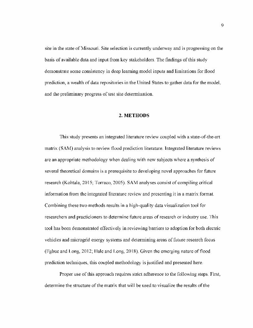
2. METHODS
This study presents an integrated literature review coupled with a state-of-the-art
matrix (SAM) analysis to review flood prediction literature. Integrated literature reviews
are an appropriate methodology when dealing with new subjects where a synthesis of
several theoretical domains is a prerequisite to developing novel approaches for future
research (Kohtala, 2015; Torraco, 2005). SAM analyses consist of compiling critical
information from the integrated literature review and presenting it in a matrix format.
Combining these two methods results in a high-quality data visualization tool for
researchers and practicioners to determine future areas of research or industry use. This
tool has been demonstrated effectively in reviewing barriers to adoption for both electric
vehicles and microgrid energy systems and determining areas of future research focus
(Egbue and Long, 2012; Hale and Long, 2018). Given the emerging nature of flood
prediction techniques, this coupled methodology is justified and presented here.
Proper use of this approach requires strict adherence to the following steps. First,
determine the structure of the matrix that will be used to visualize the results of the

10
integrated literature review. The SAM presented in this study consists of columns
dedicated to author(s), year, method, data, and limitations. These dimensions were chosen
to identify trends and limitations in the literature to inform future research direction. The
SCOPUS database was used to retrieve peer-reviewed journal articles under the search
terms “flood” AND “prediction”. Search critiera was refined to include peer-reviewed
sources only. 18 articles out of nearly 3000 published from 2012-2019 were selected to
demonstrate a breadth of methodologies. Reliability of findings increases as more articles
are added to the analysis. Therefore, the findings presented here are inconclusive, but
provide a preliminary basis for future research direction. The results of the integrated
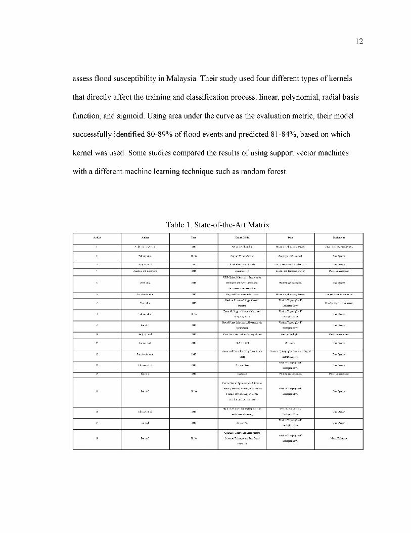
literature review and SAM analysis are presented in Table 1.
The second part of this study uses the findings of the integrated literature review
and the SAM analysis as model inputs to determine the type and amount of data that is
required. Datasets from USGS, NOAA, and USDA are reviewed here including tools
they use. The concurrent findings of the integrated literature review and SAM are then
synthesized with the review of data sources to review suitable test locations in one urban
and one rural area of Missouri.
3. RESULTS AND DISCUSSION
A summary of the SAM analysis can be found in Table 1. The results show that
no single method or model dominates the literature, but there are clear trends related to
data and its quality as a limitation in current models. This limitation could be addressed

11
by gathering more data, increasing the interval of measurement, or improving the quality
of instrument used to gather the data. Table 2 presents the most prevalent model inputs
and their frequency of use in the articles that used machine learning or deep learning
techniques. Based upon these findings, the remainder of this section will be divided into
subsections that better organize the information: Deep Learning Methods, Other
Methods, Data, and Review of Data Sources.
3.1. DEEP LEARNING METHODS AND DATA
There is perhaps some confusion between the term artificial intelligence, machine
learning, and deep learning. Artificial intelligence is any program that exhibits intelligent
behavior such as the ability to sense, reason, act, and adapt. Machine learning is the
process by which algorithms improve their performance through exposure to data over
time. Deep learning is a more comprehensive form of machine learning where
multilayered neural networks learn from large amounts of data (Intel, 2017).
Nine of the 18 articles included in the SAM used machine learning methodologies
such as support vector machine, random forest, decision trees, and artificial neural
networks. The purpose of this study is to investigate the use of these techniques in flood
prediction modeling. Brief summaries of a technique are given here, but readers seeking
to better understand model theory are directed to the references.
Support vector machines are an emerging approach in flood prediction studies.
This technique is a supervised machine learning algorithm that finds a hyperplane that
divides the dataset into two classes. Tehrany et al. (2015a) used this methodology to
12
assess flood susceptibility in Malaysia. Their study used four different types of kernels
that directly affect the training and classification process: linear, polynomial, radial basis
function, and sigmoid. Using area under the curve as the evaluation metric, their model
successfully identified 80-89% of flood events and predicted 81-84%, based on which
kernel was used. Some studies compared the results of using support vector machines
with a different machine learning technique such as random forest.

13
Table 2. Dominant Model Inputs as a PercentageM odel Input %
S l o p e 8 9 %
S t r e a m P o w e r I n d e x 8 9 %
T o p o g r a p h i c W e t n e s s I n d e x 8 9 %
D i g i t a l E l e v a t i o n M o d e l 8 9 %
C u r v a t u r e 7 8 %
E l e v a t i o n 6 7 %
D i s t a n c e f r o m r i v e r 6 7 %
S o i l T y p e 6 7 %
R a i n f a l l 5 6 %
N o r m a l i z e d D i f f e r e n c e V e g e t a t i o n I n d e x 4 4 %
The random forest algorithm draws multiple samples using the bootstrap
resampling method and then builds classification trees for each bootstrap sample.
Ultimately, forecast classification trees are combined and voting determines final
classification results. Wang et al. (2015) used this methodology and compared its results
to the support vector machine for the same data for flood hazard risk assessment in
China. Their results demonstrate that the percentage error rate decreased as sample size
and number of decision trees increased. The correlation coefficient between random
forest and support vector machine was 0.9156, demonstrating comparable performance in
most cases.
Decision trees consist of breaking down data into increasingly smaller subsets
using if-then-else rules. The structure of the decision-making process resembles that of a
tree with increasing depth resulting in a more complex and fit model. Khosravi et al.
(2018) used four different decision tree algorithms, logistic model trees, reduced error

14
pruning trees, naive bayes trees, and alternating decision trees to model flash flood
susceptibility in Iran. Area under the curve was again used to evaluate model
performance. Their study found that alternating decision trees achieved an area under the
curve value of 0.976.
Artificial neural networks are a widely used machine learning algorithm due to
their computational efficiency. However, the model technique has weaknesses resulting
in poor predictive capabilities due to dataset characteristics. Bui et al. (2016) took the
integrated fuzzy inference system (Chang and Tsai, 2016; Guclu and Sen, 2016; Lohani
et al., 2012; Shu and Ouarda, 2008) and added two metaheuristic algorithms,
evolutionary genetic and particle swarm, to optimize it. The model was tested on a high-
frequency tropical cyclone area in Vietnam. The model was compared to other models
using decision trees, neural nets, random forest, support vector machine, and adaptive
neuro fuzzy inference system. Their findings demonstrate that the fuzzy inference system
model with metaherustic optimization outperformed other models in terms of prediction
capability with a superior area under the curve value.
All the inputs in Table 2 achieved coverage in the literature greater than 50% with
the exception of normalized difference vegetation index (NDVI). The lack of presence in
the literature is likely attributable to sensors used in the data collection process.
Specifically, NDVI is a variable almost exlusively used by studies that rely on land
satellite imagery. This input was included to capture unique runoff characteristics.
However, NDVI would only capture those characteristics in a setting where vegetation
was present (i.e. rural). Further investigation into general runoff values is required to

15
encompass that portion of a flood event. Model input exclusion here does not signify that
it is unnecessary. The authors of these studies were thorough in their use and elimination
of flood mechanisms that included comprehensive literature reviews and multicollinearity
tests to ensure that there was no correlation among independent variables.
Flood prediction literature, especially pertaining to the use of machine learning
and deep learning methodologies, has seen a considerable increase in publications
recently. This can largely be attributed to an increase in the frequency and magnitude of
flooding events worldwide, data availability, and improvements in computing power.
These techniques will be enhanced as the amount and quality of available data improves.
3.2. OTHER METHODS
The focus of this study is to investigate the potential of machine learning
techniques to predict flood events and the data required to do so. However, nine of the 18
articles covered in the SAM deployed methods unrelated to machine learning. This
section will briefly examine those articles to determine if key findings could be integrated
into future model development.
As data quality emerged as a limitation, it became apparent that further research
into quality improvement studies was required. Therefore, conversations with industry
professionals indicated work being done in part by the Center of Excellence for
Geospatial Information Science within USGS. Their work primarily deals with improving
the National Map, a highly detailed and multi-layered topographic map for the United
States. Anderson-Tarver et al. (2012) presented an algorithm that delineates cartographic

16
centerlines. This process enriches the hydrographic database for base mapping at smaller
scales. This contribution is important due to challenges with extracting important features
in the absence of available information regarding stream order, channel depth, or flow
rate. Further improvement to the national map was achieved when Stanislawski et al.
(2015) proposed the coefficient of line correspondence metric that assessed the similarity
of two different sets of linear features. Their study improved the national hydrography
dataset by making it more consistent and suitable for hydrologic investigations by
thinning flowlines where content is too dense to achieve the resolution required. These
studies represent data source improvements to enhance investigation efforts.
The remaining papers present flood prediction methodologies without the use of
machine learning techniques. Sampson et al. (2015) presented a high-resolution global
flood hazard model framework. The framework consisted of the following workflow:
global terrain data, extreme flow generation, global river network and geometry, flood
defenses, computational hydraulic engine, and automation framework. Their model used
similar data compared to the machine learning studies including rainfall data,
hydrography data, and data extracted from digital elevation models. Their findings
presented a model that was capable of capturing two thirds to three quarters of flooded
areas in the local benchmark data. Yucel et al. (2015) used an integrated model that
consisted of a numerical weather prediction model and fully distributed hydrologic and
hydraulic models to simulate heavy rain induced flood events over mountainous basins in
Turkey. Their model reasonably simulated features of flood events such as volume, peak
flow rate, and timing. These studies represent a different yet effective approach to

17
predicting floods. Key findings pertaining to data quality improvement and model
frameworks used can be effectively integrated into deep learning methodologies to
improve model performance and provide a basis for comparison of model results.
4. DATA SOURCES
Large amounts of high-quality data are prerequisite in implementing deep
learning techniques. Based on the results of the integrated literature review and SAM
analysis, the model inputs listed in Table 2 were determined. Fortunately, the United
States has several data repositories made available by USGS, NOAA, and USDA. The
USGS provides the highest quality digital elevation models available from which other
model inputs can be extracted by geographic information system techniques. Specifically,
slope, curvature, elevation, stream power index, topographic wetness index, and
normalized difference vegetation index. Figure 1 demonstrates 1-m digitial elevation
model (DEM) coverage for the state of Missouri constructed from USGS data.
The hydrograph is separated into minor, moderate, and major flood categories. As
the graph suggests, the Missouri River was in a state of major flooding at this location on
26 May 2019 and was predicted to remain at least minorly flooded until Tuesday, 4 June
2019, Lastly, USDA provides soil type through their web soil survey database. These
data sets represent a wealth of available data that if used in concert could prove effective
in developing a deep learning model to enhance flood prediction efforts.

18
St. Joseph Area DEM 1OWA Burlington ~ \ P e o r . a
Hannibal Area DEM p**,,.
ILLIN O ISl,Columbia Area DEM
Spnngfir
MacSft,
S Ttaman™>r (MjSorksNevada Area DEM
Ste Genevieve Area DEM —
SpringfieldCape Girardeau Area DEM ------UPo' The
I 'ir /.i; ..-.--
9168. -94 6692
Figure 1. 1-m DEM Data Coverage in Missouri
Figure 2. NOAA Hydrograph for Missouri River at Glasgow
Flow (kefs)

19
5. CONCLUSIONS AND FUTURE WORK
This study presented the findings of an integrated literature review and SAM
analysis of 18 peer-reviewed flood prediction studies. A larger sample size of studies
would markedly enhance the quality of the findings presented here which would provide
a more reliable assessment of the literature and is the subject of future work. Nine of the
articles used machine learning or deep learning techniques such as support vector
machine, decision trees, random forest, and artificial neural networks. There were two
observable trends among these articles. First, a relative commonality existed regarding
model inputs detailed further in Table 2. Second, data quality was regularly identified as
a limitation due to deep learning requiring a large amount of high-quality data. Data
available from USGS, NOAA, and the USDA were then reviewed and shown to possess
the data required to build a deep learning model capable of accurately predicting floods.
Other models were also reviewed and useful frameworks such as that posited by
Sampson et al. (2015) were observed. Overall, these findings demonstrate that machine
learning and deep learning methods are an emerging and effective strategy for flood
prediction dependent upon available data.
Using these findings, determination of one urban and one rural test site are
underway. The St. Louis area has been chosen as the urban test site due to historic
flooding events and the vast amounts of data available. The choice of rural location is still
in progress but will be somewhere within the Meramec Basin subject to discussions with
key stakeholders and subject matter experts. The difficulty in selecting a rural test site is

20
due in large part to the lack of sufficient data to conduct a deep learning technique.
Finally, a deep learning technique will be chosen based upon further consideration of the
available options and comparison of performance from multiple models.
The findings presented here can be used two-fold. First, researchers can use these
findings to inform future research direction by improving upon models reviewed here or
enhancing the quality of available data. Second, emergency response managers can use
the findings here as a starting point for incorporating machine learning and deep learning
flood prediction models as part of their strategic management of resources when flooding
events become highly probable. Ultimately, as data availability and quality improve the
use of machine learning and deep learning methodologies will become commonplace
resulting in dramatic reductions regarding the risk, cost, and time considerations regularly
associated with flooding events.
ACKNOWLEDGEMENTS
The authors gratefully acknowledge partial support for this project through
funding provided by the Missouri Department of Transportation, TR201912, and the
Mid-America Transportation Center, 25-1121-0005-130. The authors would also like to
acknowledge the anonymous reviewers for their contributions to the improvement of this
paper.
21
REFERENCES
Anderson-Tarver, C., Gleason, M., Buttenfield, B., & Stanislawski, L. (2012). Automated Centerline Delineation to Enrich the National Hydrography Dataset. Proceedings of the 7th International Geographic Information Science Conference. 15-28.
Associated Press. (2019, March 19). U.S. M idw est F lood ing C ost E stim a ted a t M ore than $3B. Retrieved from: https://www.cbc.ca/news/world/midwest-floods-economic- cost-1.5068037
Berghuijs, W. R., Woods, R. A., Hutton, C. J., & Sivapalan, M. (2016). Dominant flood generating mechanisms across the United States. G eophysical R esearch Letters, 43(9), 4382-4390. https://doi.org/10.1002/2016GL068070
Bui, D. T., Ngo, P. T. T., Pham, T. D., Jaafari, A., Minh, N. Q., Hoa, P. V., & Samui, P. (2019a). A novel hybrid approach based on a swarm intelligence optimized extreme learning machine for flash flood susceptibility mapping. Catena, 179(April), 184196. https://doi.org/10.1016Zj.catena.2019.04.009
Bui, D. T., Tsangaratos, P., Ngo, P. T. T., Pham, T. D., & Pham, B. T. (2019b). Flash flood susceptibility modeling using an optimized fuzzy rule based feature selection technique and tree based ensemble methods. Science o f the Total Environm ent, 668, 1038-1054. https://doi.org/10.10167j.scitotenv.2019.02.422
Chang, F.-J., Tsai, M.-J., (2016). A nonlinear spatio-temporal lumping of radar rainfall for modeling multi-step-ahead inflow forecasts by data-driven techniques. J. H ydrol. 535, 256-269. http://dx.doi.org/10.1016/jjhydrol.2016.01.056.
Costabile, P., & Macchione, F. (2015). Enhancing river model set-up for 2-D dynamic flood modelling. E nvironm enta l M odelling a n d Software, 67, 89-107. https://doi.org/10.1016/j.envsoft.2015.01.009
Dorigo, W., Wagner, W., Albergel, C., Albrecht, F., Balsamo, G., Brocca, L., ...Lecomte, P. (2017). ESA CCI Soil Moisture for improved Earth system understanding: State-of-the art and future directions. Rem ote Sensing o f Environm ent, 203, 185-215. https://doi.org/10.1016/j.rse.2017.07.001
Du, W., Chen, N., Yuan, S., Wang, C., Huang, M., & Shen, H. (2019). Sensor web -Enabled flood event process detection and instant service. E nvironm enta l M odelling & Software, 117(December 2018), 29-42. https://doi.org/10.1016/j.envsoft.2019.03.004

22
Egbue, O., Long, S. (2012). C ritical Issues in the Supply Chain o f L ith ium fo r E lectric Vehicle Batteries. Eng. Manag. J., vol. 24, no. 3, pp. 52-62.
FEMA. (2017, July 5). The B IG C ost o f Flooding. Retrieved from: https://www.fema.gov/media-library/assets/documents/132744
FEMA. (2019, May 10). D ata Visualization: H istorica l F lo o d R isk a n d Costs. Retrieved from: https://www.fema.gov/data-visualization-floods-data-visualization
Gu.lu, Y.S., S_en, Z., (2016). Hydrograph estimation with fuzzy chain model. J. Hydrol. 538, 587-597. http://dx.doi.org/10.1016/jjhydrol.2016.04.057.
Hale, J., Long, S. (2018). Determining Microgrid Energy Systems Dynamic Model Inputs Using a SAM Analysis. Proeedings of the 39th International Annual Conference of the American Society for Engineering Management. 596-604.
Hu, C., Wu, Q., Li, H., Jian, S., Li, N., & Lou, Z. (2018). Deep learning with a long short-term memory networks approach for rainfall-runoff simulation. Water (Switzerland), 10(11), 1-16. https://doi.org/10.3390/w10111543
Intel. (2017, September 7). Infographic: G et S ta rted w ith A I D evelopm ent Today. Retrieved from: https://software.intel.com/en-us/articles/infographic-get-started- with-ai-development-today
Khosravi, K., Pham, B. T., Chapi, K., Shirzadi, A., Shahabi, H., Revhaug, I., Tien Bui, D. (2018). A comparative assessment of decision trees algorithms for flash flood susceptibility modeling at Haraz watershed, northern Iran. Science o f the Total Environm ent, 627, 744-755. https://doi.org/10.1016Zj.scitotenv.2018.01.266
Khosravi, K., Shahabi, H., Pham, B. T., Adamowski, J., Shirzadi, A., Pradhan, B.,Prakash, I. (2019). A comparative assessment of flood susceptibility modeling using Multi-Criteria Decision-Making Analysis and Machine Learning Methods. Journa l o f H ydrology, 573(February), 311-323. https://doi.org/10.1016/jjhydrol.2019.03.073
Kohtala, C. (2015). Addressing sustainability in research on distributed production: An integrated literature review. Journa l o f C leaner Production, 106, 654-668. https://doi.org/10.1016/jjclepro.2014.09.039
Li, Z., Yang, D., Gao, B., Jiao, Y., Hong, Y., & Xu, T. (2014). Multiscale Hydrologic Applications of the Latest Satellite Precipitation Products in the Yangtze River Basin using a Distributed Hydrologic Model. Journa l o f H ydrom eteorology, 16(1), 407-426. https://doi.org/10.1175/jhm-d-14-0105.!

23
Lohani, A., Kumar, R., Singh, R., (2012). Hydrological time series modeling: a comparison between adaptive neuro-fuzzy, neural network and autoregressive techniques. J. H ydrol. 442, 23-35.
NOAA. (2019, May 26). Hydrograph. Retrieved from: https://water.weather.gov/ahps/
Rahmati, O., Zeinivand, H., & Besharat, M. (2016). Flood hazard zoning in Yasooj region, Iran, using GIS and multi-criteria decision analysis. Geomatics, N a tura l H azards a n d R isk, 7(3), 1000-1017. https://doi.org/10.1080/19475705.2015.1045043
Rusk, N. (2015). Deep learning. N ature M ethods, 13(1), 35. https://doi.org/10.1038/nmeth.3707
Sampson, C., Smith, A., Bates, P., Neal, J., Alfieri, L., & Freer, J. (2015). A high-resolution global flood hazard model Christopher. W ater Resources, 51, 7358-7381. https://doi.org/10.1002/2015WR016954.
Shu, C., Ouarda, T., (2008). Regional flood frequency analysis at ungauged sites using the adaptive neuro-fuzzy inference system. J. H ydrol. 349 (1), 31-43.
Stanislawski, L. V., Survila, K., Wendel, J., Liu, Y., & Buttenfield, B. P. (2018). An open source high-performance solution to extract surface water drainage networks from diverse terrain conditions. C artography a n d G eographic Inform ation Science, 45(4), 319-328. https://doi.org/10.1080/15230406.2017.1337524
Tehrany, M. S., Pradhan, B., & Jebur, M. N. (2015a). Flood susceptibility analysis and its verification using a novel ensemble support vector machine and frequency ratio method. Stochastic E nvironm enta l R esearch a n d R isk A ssessm ent, 29(4), 11491165. https://doi.org/10.1007/s00477-015-1021-9
Tehrany, M. S., Pradhan, B., Mansor, S., & Ahmad, N. (2015b). Flood susceptibility assessment using GIS-based support vector machine model with different kernel types. Catena, 125, 91-101. https://doi.org/10.1016/jxatena.2014.10.017
Tian, J., Liu, J., Yan, D., Ding, L., & Li, C. (2019). Ensemble flood forecasting based on a coupled atmospheric-hydrological modeling system with data assimilation. Atm ospheric Research, 224(1), 127-137. https://doi.org/10.1016ZJ.ATMOSRES.2019.03.029

24
Tien Bui, D., Pradhan, B., Nampak, H., Bui, Q. T., Tran, Q. A., & Nguyen, Q. P. (2016). Hybrid artificial intelligence approach based on neural fuzzy inference model and metaheuristic optimization for flood susceptibilitgy modeling in a high-frequency tropical cyclone area using GIS. Journa l o f H ydrology, 540, 317-330. https://doi.org/10.1016/jjhydrol.2016.06.027
Torraco, R. J. (2016). Writing Integrative Literature Reviews. H um an ResourceD evelopm ent Review , 15(4), 404-428. https://doi.org/10.1177/1534484316671606
Wang, Z., Lai, C., Chen, X., Yang, B., Zhao, S., & Bai, X. (2015). Flood hazard risk assessment model based on random forest. Journa l o f H ydrology, 527, 1130-1141. https://doi.org/10.1016/jjhydrol.2015.06.008
Yucel, I., Onen, A., Yilmaz, K. K., & Gochis, D. J. (2015). Calibration and evaluation of a flood forecasting system: Utility of numerical weather prediction model, data assimilation and satellite-based rainfall. Journa l o f H ydrology, 523, 49-66. https://doi.org/10.1016/jjhydrol.2015.01.042

25
II. USING TREND EXTRACTION AND SPATIAL TRENDS TO IMPROVE FLOOD MODELING AND CONTROL
Jacob Hale1, Suzanna Long1, Vinayaka Gude2, Steven M. Corns1
department of Engineering Management and Systems Engineering, Missouri University of Science and Technology, Rolla, MO 65409
department of Arts and Media, Louisiana State University Shreveport, Shreveport, LA71115
ABSTRACT
Effective management of flood events depends on a thorough understanding of
regional geospatial characteristics, yet data visualization is rarely effectively integrated
into the planning tools used by decision makers. This chapter considers publicly available
data sets and data visualization techniques that can be adapted for use by all community
planners and decision makers. A long short-term memory (LSTM) network is created to
develop a univariate time series value for river stage prediction that improves the
temporal resolution and accuracy of forecasts. This prediction is then tied to a
corresponding spatial flood inundation profile in a geographic information system (GIS)
setting. The intersection of flood profile and affected road segments can be easily
visualized and extracted. Traffic decision makers can use these findings to proactively
deploy re-routing measures and warnings to motorists to decrease travel-miles and risks
such as loss of property or life.

26
1. INTRODUCTION
Floods are the most frequently occurring natural disaster. A flood event occurs
when stream flows exceed the natural or artificial confines at any point along a stream
[1]. This is often due to heavy rainfall, ocean waves coming on shore, rapid snow
melting, or failure of manmade structures such as dams or levees [2]. From 1998-2017,
flood events affected more than two billion people globally [3]. Disasters of this
frequency and magnitude are typified by extreme costs to governments. In 2019, historic
flooding across Missouri, Arkansas, and the Mississippi River basin resulted in an
estimated cost of 20 billion dollars [4]. These estimates typically do not reflect indirect
costs such as added travel-miles and the subsequent loss of time. Further, floods are
among the most deadly natural disasters. From 2010-2020, floods resulted in the fatalities
of 1089 people in the United States [5]. A majority of these deaths were comprised of
motorists. Therefore, urban planners such as traffic decision makers are tasked with
proactively deploying resources that minimize motorist risk exposure. At present, traffic
decision makers rely on static flash flood inundation profiles related to discrete rainfall
events. These profiles are often created through multiagency cooperation efforts such as
[6]. Some studies have begun to generate dynamic flood inundation data visualizations
based on these profiles [7]. Additionally, integrated approaches that use machine learning
and geographic information systems (GIS) to track changes in critical infrastructure over
time are emerging as powerful decision support tools [8]. However, there is limited use of
state-of-the-art time series prediction models to generate dynamic data visualizations in a

27
GIS setting for improved flood management. This book chapter explores the integration
of publicly available data and machine learning models to address this gap in the
literature.
Precise determination of when and where to deploy re-routing measures is a
complex task. One approach that improves planning effectiveness is to integrate time
series characteristics of river behavior and corresponding spatial flood profile. In this
chapter, a univariate time series prediction of river stage is conducted that improves the
temporal resolution and accuracy of publicly available forecasts. This prediction is then
tied to a corresponding spatial flood inundation profile in a GIS setting. The resulting
geospatial deep learning model provides a data visualization tool that traffic decision
makers can use to proactively manage road closures in the event that a flood is likely to
occur. The first section provides an overview of relevant river behavior that causes
flooding. State-of-the-art trend extraction and prediction techniques are then presented
and tied to geospatial use cases. The methodology section presents the data used, time
series prediction model selected, and geoprocessing procedures required for data
visualization using GIS software. Next, an illustrative example is provided for a
frequently flooded intersection in Missouri. A discussion section is provided that
positions the findings in the context of improving traffic management in the event of a
flood. Lastly, a conclusion is given that summarizes the key findings and outlines model
limitations and future work.

28
2. A GEOSPATIAL DEEP LEARNING APPROACH
Two key characteristics of streams that relate to flood events are stream stage and
streamflow. Stream stage refers to height (ft) of the stream and streamflow corresponds to
discharge (ft3/s) or alternatively, volumetric flowrate. Typically, governmental
organization such as the United States Geological Survey maintain a network of sensors
that monitor these characteristics over time for various stream segments. The National
Weather Service classifies flood categories into four groups based on stream stage:
Action Stage, Flood Stage, Moderate flood Stage, and Major Flood Stage [9]. These
values vary for a given segment of stream based on analysis of previous floods, local
topography, and underlying geological properties.
Given that stage is monitored over time, the use of time series forecasting
methods to predict stage values is appropriate. There are two modelling approaches that
are useful in this context: statistical and computational intelligence. Statistical models use
historical data to identify underlying patterns to predict future values [10]. Some
commonly used techniques for flood forecasting include simple exponential smoothing
[11], autoregressive moving average [12], and autoregressive integrated moving average
[13]. However, one shortcoming of these approaches is lack of scalability as the quantity
and complexity of data increases [14]. An alternative approach that addresses these issues
is computational intelligence. A key feature of computational intelligence approaches is
the capacity to manage complexity and non-linearity without needing to understand
underlying processes [15]. In summary, statistical methods rely on precise underlying

29
relationships and exhibit decreased performance as the number of variables increases
whereas computational intelligence approaches identify patterns using large amounts of
training data to establish a model capable of accurate predictions [16]. Some commonly
used flood forecasting computational intelligence models include support vector
machines [17], artificial neural networks [18], and deep learning [19]. Further, they have
demonstrated superior performance when compared to conventional statistical modelling
approaches for flood prediction studies. LSTM models have explicitly shown promising
results in time series contexts. Therefore, LSTM models provide a state-of-the-art trend
extraction and prediction technique regarding stream stage values.
Stream stage values are categorized based on resulting flood severity. The
physical reality of these categories is the spatial extent of the flooding event often
referred to as a flood inundation map [20]. These maps provide decision makers with a
useful visual reference to determine what specifically has been affected by a flood event.
An area of research, data visualization, and practical application that has not been fully
investigated is the integration of computational intelligence stream stage predictions with
geospatial flood inundation maps. The methodology provided in the following section
addresses this gap.
3. METHODOLOGY
This section consists of three parts: LSTM prediction of stream stage, data
required, and geoprocessing procedures. First, a brief overview of LSTM will be given.
30
This will include explanatory figures and relevant mathematical formulas. Second, data
required to conduct the LSTM prediction of stream stage will be procured. Flood
inundation imagery and road network data will also be obtained. Lastly, data will be
uploaded to a GIS software and processed for end use by traffic decision makers. An
illustrative example is presented in the next section.
3.1. LSTM PREDICTION OF STREAM STAGE
Stream stage prediction is a time series forecasting procedure that is dependent on
previous data to predict future values. As the quantity and quality of data continues to
increase, more powerful computational approaches can be applied to prediction problems.
The results of the literature review demonstrated that deep learning approaches, namely
LSTM networks, are increasingly being applied to these problems.
Deep learning is an extension of the conventional neural network by adding
additional layers and layer types. Figure 1 provides a visual comparison of the two
approaches [21]. The simple neural network (left) consists of a single input layer, hidden
layer, and output layer. Alternatively, the deep learning neural network (right) has one
input layer followed by three successive hidden layers that ultimately feed into a final
output layer. This configuration has generated superior performance in capturing
complex relationships.

31
Simple Neural Network Deep Learning Neural Network
Figure 1. Simple Neural Network vs. Deep Learning Neural Network
However, neither approach retains previous time step information. Recurrent
neural networks (RNNs) were introduced to address this limitation. LSTM networks are
the deep learning variant of RNNs. All figures and mathematical formulation are
borrowed from [15]. The primary benefit of LSTM networks is the capacity to retain
longer term information. This is accomplished by removing and adding information
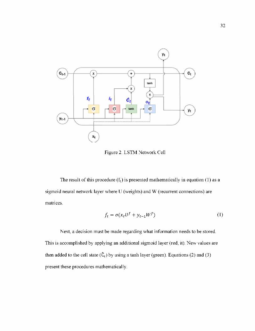
determined by a series of ‘gates’ and vector operations. Figure 2 provides a visual
representation of an LSTM cell. The first gate, illustrated in yellow, generates a value
between 0 and 1 using the current input (xt) and output from the previous step (yt-1) that
determines how much information is passed on (forget gate). A zero corresponds to no
information transfer whereas a one represents a complete transfer.
32
Figure 2. LSTM Network Cell
The result of this procedure (ft) is presented mathematically in equation (1) as a
sigmoid neural network layer where U (weights) and W (recurrent connections) are
matrices.
f t = ° ( .x t Uf + y t - i W f ) (1)
Next, a decision must be made regarding what information needs to be stored.
This is accomplished by applying an additional sigmoid layer (red, it). New values are
then added to the cell state (Ct) by using a tanh layer (green). Equations (2) and (3)
present these procedures mathematically.
33
it = a ( x t Ul + y t- i W l) (2)
Ct = tanh (x t U9 + y t - 1 W 9 ) (3)
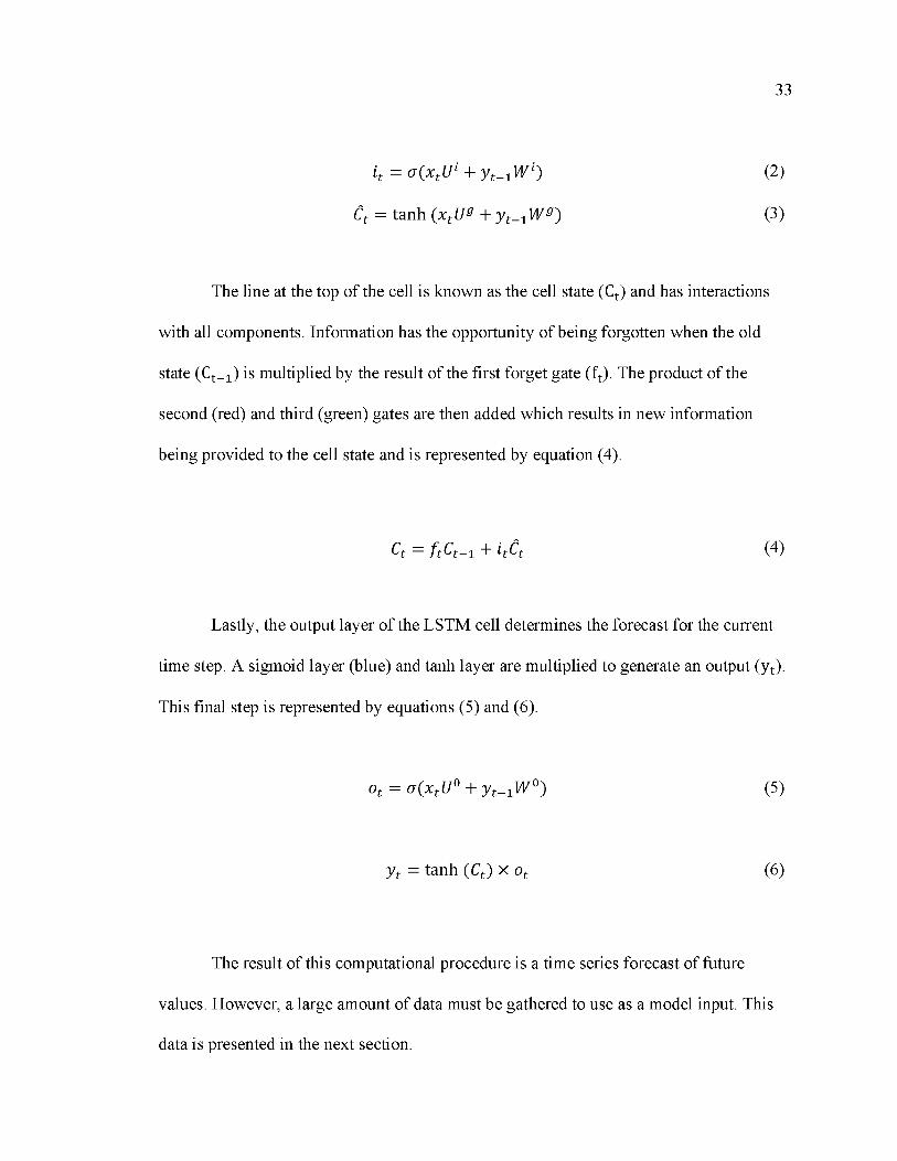
The line at the top of the cell is known as the cell state (Ct) and has interactions
with all components. Information has the opportunity of being forgotten when the old
state (Ct-1) is multiplied by the result of the first forget gate (ft). The product of the
second (red) and third (green) gates are then added which results in new information
being provided to the cell state and is represented by equation (4).
Ct = f t ^ t - i + h ^ t (4)
Lastly, the output layer of the LSTM cell determines the forecast for the current
time step. A sigmoid layer (blue) and tanh layer are multiplied to generate an output (yt).
This final step is represented by equations (5) and (6).
ot = a ( x t U0 + y t- i W 0) (5)
y t = tanh (Ct ) x ot (6)
The result of this computational procedure is a time series forecast of future
values. However, a large amount of data must be gathered to use as a model input. This
data is presented in the next section.
34
3.2. DATA REQUIRED
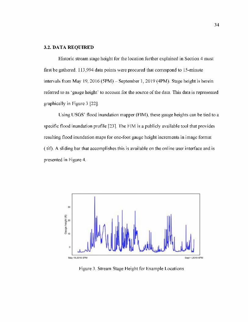
Historic stream stage height for the location further explained in Section 4 must
first be gathered. 113,994 data points were procured that correspond to 15-minute
intervals from May 19, 2016 (5PM) - September 1, 2019 (4PM). Stage height is herein
referred to as ‘gauge height’ to account for the source of the data. This data is represented
graphically in Figure 3 [22].
Using USGS’ flood inundation mapper (FIM), these gauge heights can be tied to a
specific flood inundation profile [23]. The FIM is a publicly available tool that provides
resulting flood inundation maps for one-foot gauge height increments in image format
(.tif). A sliding bar that accomplishes this is available on the online user interface and is
presented in Figure 4.
Figure 3. Stream Stage Height for Example Locations

35
^ Flood Tools Hydrograph as Services and Data Q More Info
Selected gage height: 11 feet
Current ConditionsGage height: 8.99 feet
Discharge: 616 cfs
USGS Site No: 07019130 NWS Site ID: vllm7
Figure 4. FIM Sliding Gauge Height Tool
An example of a flash flood inundation profile being uploaded to a GIS software
is provided in Figure 5. Purple lines correspond to road network data derived from the
National Transportation Dataset [24]. Blue raster (grids of pixels) imagery denotes the
depth of water at discrete locations where darker blue reflects deeper water. Useful
geoprocessing techniques that generate actionable decision support tools are presented in
the next section.
3.3. GEOPROCESSING PROCEDURES
Traffic decisions makers are tasked with identifying flood affected road segments.
In Figure 5, it can be observed that the flood inundation profile does overlap certain road
segments. Relying on visual inspection alone is time consuming and prone to
inaccuracies due to human error. A solution to this issue is the application of a set of

36
straightforward geoprocessing tools that are built-in to most GIS softwares: conversion
and intersection.
Figure 5. Flood Inundation Profile Example
Some tools do not allow raster and vector data layer interoperability. Therefore, it
is necessary to convert one of the data layers to establish a consistent data type. One
approach is to convert the raster layer into a vector layer using the conversion tool within
ArcGIS. Figure 6 illustrates the result of this operation. The flood inundation profile has
been converted into several points at 1-m increments. This spatial resolution can be
modified by the user. The road network has been changed from its previous color to
improve readability.

37
Figure 6. Raster Layer Conversion Example
Once the raster layer has been converted into vector format, it is eligible for use as
an input layer for the intersection tool. The intersection tool generates a point at every
location where there is an intersection between the input layers. In the next section, an
illustrative example is provided to demonstrate the effectiveness of the methodology
presented.
4. ILLUSTRATIVE EXAMPLE
Valley Park, Missouri is located at the intersection of I-44 and State Route 141.
This location is the setting for the example figures presented previously. The Meramec
River winds through this area and has regularly flooded in recent years. In 2017, the river
exceeded its banks and caused significant damage to the surrounding area as seen in

38
Figure 7. This location provides a suitable candidate to test the methodology presented
given the extent of the flood event and data availability.
Meram'ejClH i v.erf (norma 11 V/)l
Eloocl fQ v.e r,t I owlO rit <53 I ̂ 4!4i
Figure 7. Meramec River Flood in 2017 [25]
First, data is gathered from a nearby stream gauge. Figure 8 provides a
geographical point of reference for the gauge denoted by a green square with respect to I-
44 and State Route 141. The data presented in Figure 5 is then procured and used as an
input for the LSTM network. Figure 9 presents the prediction results of the LSTM model
superimposed on the actual data for May 19, 2016-September 1, 2019.
The actual data (blue) can be observed deviating from the prediction results for
the training (orange) and testing (green) results of the LSTM network. A lack of
discrepancy between the actual data and predictions demonstrates the model’s
effectiveness. Further, it is useful to determine how the prediction compares with publicly
available forecasts for the same location. USGS provides a forecast every six hours.

39
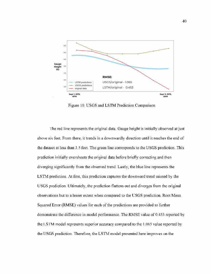
Alternatively, the LSTM network provides 24 predictions in the same period. Figure 10
provides a comparison of the prediction provided by USGS and the LSTM model for
September 1, 2019 (6PM) - September 3, 2019 (6AM).
Figure 8. Gauge Location [9]
Figure 9. LSTM Training and Testing Results
40
G a u g eH eigh t
R M S E :
USCS/original -1.065LSTM predictionsU S G S predictions
LSTM/original - 0.453original data
S e p t 1, 2019 S e p t 3 , 20196 P M BAM
Figure 10. USGS and LSTM Prediction Comparison
The red line represents the original data. Gauge height is initially observed at just
above six feet. From there, it trends in a downwardly direction until it reaches the end of
the dataset at less than 3.5 feet. The green line corresponds to the USGS prediction. This
prediction initially overshoots the original data before briefly correcting and then
diverging significantly from the observed trend. Lastly, the blue line represents the
LSTM prediction. At first, this prediction captures the downward trend missed by the
USGS prediction. Ultimately, the prediction flattens out and diverges from the original
observations but to a lesser extent when compared to the USGS prediction. Root Mean
Squared Error (RMSE) values for each of the predictions are provided to further
demonstrate the difference in model performance. The RMSE value of 0.453 reported by
the LSTM model represents superior accuracy compared to the 1.065 value reported by
the USGS prediction. Therefore, the LSTM model presented here improves on the

41
accuracy of publicly available forecasts and can be used as an input for the flood
inundation tool.
Valley Park has 43 flood inundation profiles available in one-foot increments
from 11-54 feet. The highest stage value recorded at this location is 44.11 feet on
December 31, 2015. Figure 11 provides the flood inundation profile for 45 feet to
approximate this event. Note that 45 feet is used instead of 44. This is due to the flood
inundation profile incremental limitation and opting for a rounding approach that
provides a more conservative risk assessment. The inundation profile is then converted to
point format and intersected with the road network as illustrated by Figure 12.
Figure 11. Flood Inundation Profile for 45ft. Stage Value for Valley Park, Missouri

42
Figure 12. Flood Affected Road Segments for Flood Inundation Profile Corresponding to 45ft. Stage Value for Valley Park, Missouri
5. DISCUSSION
At present, urban planners such as traffic decision makers rely on static flood
inundation maps and post hoc planning to reroute traffic if a flood occurs. This approach
puts motorists already in-transit at risk to rapidly changing road conditions. To address
these risks, a field of research has emerged to provide decision makers with real-time
decision-making tools. However, using time series prediction models that capture river
characteristics and integrating them with flood inundation profiles has receive limited
attention. The methodology provided here addresses this gap.
Traffic decision makers can use the data visualization presented in Figure 12 as a
powerful decision support tool. The flood affected road segments can be easily identified
(orange) and rerouting measures can be promptly dispatched. With the improved

43
temporal resolution and accuracy of the LSTM prediction of stage height, traffic decision
makers can deploy resources proactively to avoid unnecessary risk to motorists and
improve traffic flow. Concluding remarks, limitations, and future work are presented in
the next section.
6. CONCLUSION
Flash floods are a frequent and devastating natural disaster. The impetus to
manage these events belongs to local decision makers that work in a resource constrained
environment. To improve their decision-making effectiveness, a framework was
presented that integrates machine learning and geospatial data to extract spatial and
temporal trends using publicly available data. An illustrative example was provided to
demonstrate the effectiveness of the framework provided. Valley Park, Missouri is
located near the intersection I-44 and State Route 141. These roads represent major traffic
throughputs and persistent flooding of the Meramec River has jeopardized the safety of
motorists and the flow of commercial goods. Using 113, 994 river stage observations
procured from a nearby sensor, an LSTM network was developed to improve the
accuracy of publicly available forecasts. The result was an improvement in both the
frequency and accuracy of forecasts provided. Once the stage value is predicted it can be
tied to a spatial flood inundation profile using the publicly available FIM. Using the flood
inundation profile for 45 feet observed at Valley Park as a proxy for the historic crest at
this location, data visualization of flood affected road segments was generated in a GIS
44
setting. The key benefit of this output is the ease with which traffic decision makers can
use the results presented to inform urban planning and decision making. Traffic decision
makers can use the resulting data visualization presented here to guide real-time decision
making in the event that a river stage value is predicted to reach a flood event stage for a
specified river segment. Despite the usefulness of the findings, there remain a number of
model limitations that represent areas of future work.
Model limitations can be divided into two categories: data gathering and model
extension. Deep learning models are dependent on large amounts of data. Therefore,
sensors that collect data need to be installed and active for an extended period. The cost
to install and maintain an enlarged sensor network might be prohibitive for some
locations. Due to this fact, model implementation is limited to river locations where
sensors are already installed. Additionally, FIM coverage is confined to a small number
of locations nationwide. Similarly, to sensor coverage, if there are not already-available
flood inundation maps, then the model cannot be applied to those locations. Model
extension includes options to improve the model in a material way. One recommendation
would be to determine the best locations for road signage that will provide optimal re
routing to motorists given a finite amount of signage. Another approach would involve
working with local decision makers to determine re-routing effectiveness based on how
quickly resources are deployed given model predictions. Areas of future work not related
to model extensions include alternative prediction approaches in river networks with no
sensors and refinement of the model to account for flash floods. Each of these
45
components represent considerable opportunity for model enrichment that further
improve the decision-making effectiveness for traffic management professionals.
The results presented here demonstrate the utility of using machine learning
models and geospatial data to generate data visualization tools that key stakeholders can
use to improve planning effectiveness. As data becomes increasingly available, use of
comparably sophisticated methods can be applied to a suite of natural disaster
phenomena. The outcome of such an undertaking will be the widespread use of data
visualization tools that will reduce the risk motorists are exposed to and mitigate the
accompanying economic fallout.
ACKNOWLEDGEMENTS
This work was partially funded by the Missouri Department of Transportation,
Award Number TR201912 and the Mid-America Transportation Center, Award Number
25-1121-0005-130.
REFERENCES
[1] United States Geological Survey. Floods: Things to Know [internet]. 2019. Available from: https://www.usgs.gov/special-topic/water-science- school/science/floods-things-know?qt-science_center_objects=0#qt- science_center_objects [accessed 2019-03-15]
[2] National Severe Storms Laboratory. Flood Basics [internet]. 2019.Available from: https://www.nssl.noaa.gov/education/svrwx101/floods/ [accessed 2019-03-16]

46
[3] World Health Organization. Floods [internet]Available from: https://www.who.int/health-topics/floods#tab=tab_1 [accessed 2019-05-20]
[4] National Oceanic and Atmospheric Administration. 2010-2019: A landmark decade of U.S. billion-dollar weather and climate disasters [internet]. 2020. Available from: https://www.climate.gov/news-features/blogs/beyond-data/2010-2019- landmark-decade-us-billion-dollar-weather-and-climate [accessed 2020-1015]
[5] National Weather Service. NWS Preliminary US Flood Fatality Statistics [internet]. 2020. Available from: https://www.weather.gov/arx/usflood [accessed2020- 10-15]
[6] Dietsch, B.J., and Strauch, K.R., 2019, Flood-inundation maps of the Meramec River from Eureka to Arnold, Missouri, 2018: U.S. Geological Survey Scientific Investigations Report 2019-5004, 12 p. Available from: https://doi.org/10.3133/sir20195004.
[7] Jha MK, Afreen S. Flooding urban landscapes: Analysis using combined hydrodynamic and hydrologic modeling approaches. Water (Switzerland). 2020;12(7).
[8] Shirowzhan S, Sepasgozar SME, Li H, Trinder J, Tang P. Comparative analysis of machine learning and point-based algorithms for detecting 3D changes in buildings over time using bi-temporal lidar data. Automation in Construction. 2019Sep;105. Available from: https://doi.org/10.1016/_j.autcon.2019.102841
[9] Advanced Hydrological Prediction Service. Meramec River at Valley Park [internet]. 2019. Available from:https://water.weather.gov/ahps2/hydrograph.php?wfo=lsx&gage=vllm7 [accessed 2019-06-02]
[10] Lago J, De Ridder F, De Schutter B. Forecasting spot electricity prices: Deep learning approaches and empirical comparison of traditional algorithms. Appl Energy [Internet]. 2018;221(February):386-405. Available from: https://doi.org/10.1016/_j.apenergy.2018.02.069
[11] Papacharalampous G, Tyralis H. Hydrological time series forecasting using simple combinations: Big data testing and investigations on one-year ahead river flow predictability. J Hydrol [Internet]. 2020;590(May):125205. Available from: https://doi.org/10.1016/jjhydrol.2020.125205

47
[12] Liu J, Wang J, Pan S, Tang K, Li C, Han D. A real-time flood forecasting system with dual updating of the NWP rainfall and the river flow. Nat Hazards. 2015;77(2):1161-82.
[13] Adnan, Muhammad, X, Yuan, O, Kisi et al. Application of soft computing models in streamflow forecasting. Proceedings of the Institution of Civil Engineers - Water Management. 2019;172(3):123-124. Available from: https://doi.org/10.1680/jwama.16.00075
[14] Mosavi A, Ozturk P, Chau KW. Flood prediction using machine learning models: Literature review. Water (Switzerland). 2018;10(11): 1-40.
[15] Gude V, Corns S, Long S. Flood Prediction and Uncertainty Estimation Using Deep Learning. Water (Switzerland). 2020;12(3).
[16] Bzdok D, Altman N, Krzywinski M. Points of Significance: Statistics versus machine learning. Nat Methods [Internet]. 2018;15(4):233-4. Available from: http://dx.doi.org/10.1038/nmeth.4642
[17] Tehrany MS, Pradhan B, Jebur MN. Flood susceptibility mapping using a novel ensemble weights-of-evidence and support vector machine models in GIS. J Hydrol [Internet]. 2014;512:332-43. Available from: http://dx.doi.org/10.1016/jjhydrol.2014.03.008
[18] Shafizadeh-Moghadam H, Valavi R, Shahabi H, Chapi K, Shirzadi A. Novel forecasting approaches using combination of machine learning and statistical models for flood susceptibility mapping. J Environ Manage. 2018;217:1-11.
[19] Tien Bui D, Hoang ND, Martinez-Alvarez F, Ngo PTT, Hoa PV, Pham TD, et al. A novel deep learning neural network approach for predicting flash flood susceptibility: A case study at a high frequency tropical storm area. Sci Total Environ [Internet]. 2020;701:134413. Available from: https://doi.org/10.1016/j.scitotenv.2019.134413
[20] Papaioannou G, Vasiliades L, Loukas A. Multi-Criteria Analysis Framework for Potential Flood Prone Areas Mapping. Water Resour Manag. 2015;29(2):399- 418.
[21] Publication-ready NN-architecture schematics [internet]. 2021. Available from: alexlenail.me/NN-SVG/index.html [accessed 2021-1-27]

48
[22] United States Geological Survey. USGS 07019130 Meramec River at Valley Park, MO [internet]. 2019.Available from: https://waterdata.usgs.gov/nwis/uv?site_no=07019130 [accessed 2019-10-16] usgs 2019
[23] United States Geological Survey. Flood Inundation Mapper [internet]. 2019. Available from: https://fim.wim.usgs.gov/fim/[accessed 2019-10-18]
[24] United States Geological Survey. USGS National Transportation Dataset (NTD) Downloadable Data Collection [internet]. 2019.Available from: https://catalog.data.gov/dataset/usgs-national-transportation-dataset-ntd-downloadable-data-collectionde7d2[accessed 2019-10-22]
[25] KMOV4. Photos: Before & After Meramec River flooding [internet]. 2017. Available from: https://www.kmov.com/news/photos-before-after-meramec-river- flooding/article_fc16115e-12e2-54e6-bf84-ba1732a4dcbd.html[accessed 2019-10-25]

49
III. A COMPUTATIONAL INTELLIGENCE APPROACH TO TRANSITIONINGAN ELECTRICITY PORTFOLIO
Jacob Hale, Suzanna Long, Cihan Dagli, and Steven M. Corns
Department of Engineering Management and Systems Engineering, Missouri University of Science and Technology, Rolla, MO 65409
ABSTRACT
Greenhouse gas emissions due to fossil fuel dependence are decimating
ecosystems and communities. This is evidenced by increased frequency of extreme
weather events, rising sea levels, and erratic weather patterns to name but a few.
Therefore, it is imperative that an energy transition toward more renewable alternatives
be conducted. Energy transitions are complex processes that involve several stakeholders
and competing selection criteria. Further, criteria are usually comprised of ambiguous
terms that make it difficult to reach consensus on decisions. This work presents a meta
architecture generation model that represents the primary value delivery path for an
electricity supply system of systems. A potential meta-architecture is generated using
fuzzy associative memory and single-objective genetic algorithm. This integrated
procedure captures complexity and reduces ambiguity in the decision-making process.
The findings presented here include model representation, analysis of meta-architecture, a
unique contribution to energy transition research, and an outline of future work. These

50
results provide energy management professionals with improved information to better
guide proposed transitions.
1. INTRODUCTION
Current energy generation is largely dependent on non-renewable fossil fuels that
emit greenhouse gases when burned. Emissions contribute to the ever-growing
consequences associated with climate change. Some of the commonly cited consequences
include the increased frequency of extreme weather and climate events, damage to
infrastructure, stress on water supply and quality, disruption to the agricultural industry,
and overwhelming the capacity of ecosystems to buffer these effects. Unless a significant
transition away from fossil fuel dependence can be completed, these consequences are
expected to be exacerbated further as the global population continues to grow [1].
Climate change is a global problem that has, only recently, engendered a unified
approach from the international community through the Paris Climate Agreement [2].
Member nation goals are defined by nationally determined contributions (NDC) that
include post-2020 voluntary climate change mitigation and adaption strategies [3], [4],
[5].
Energy portfolio differences represent the presence of competing priorities among
stakeholders and different weighting schemes being applied to decisions. Additionally,
key performance criteria are often ambiguously defined leading to further complexity in
the decision-making process. Therefore, multi-criteria decision making is an effective

51
methodology to generate and assess alternative energy portfolio architectures. This paper
develops an energy transition decision methodology through the use of computational
intelligence as part of a systems software platform.
2. LITERATURE REVIEW
Most experts contend that a transition away from fossil fuel dependence and
toward renewable energy generation is imperative. However, energy planning is a
complex process that varies considerably and must be based on more than cost
considerations. The process is comprised of multiple actors and criteria that are
adversarial in nature. Georgopoulou et al. [6] presented a methodology that captured
these dynamics by accounting for actors, selection criteria, alternative strategies, and
subsequent analysis. Pohekar and Ramachandran [7] compiled one of the earliest reviews
of state-of-the-art approaches and found common trends regarding methodologies used.
The most commonly cited methods were multi-objective, multi-attribute utility theory
(MAUT), analytical hierarchy process (AHP), preference ranking organization method
for enrichment evaluation (PROMETHEE), elimination and choice translating reality
(ELECTRE), and technique for order preference by similarity to ideal solutions
(TOPSIS).
Each method has unique characteristics and strengths that make it more suitable
than the others depending on the context. ELECTRE and PROMETHEE are outranking
methods [8]. ELECTRE is based on the logic that alternatives should be comparably

52
favorable when measured across all key performance criteria [8]-[10]. PROMETHEE
conducts a pairwise comparison for each criterion and similar to ELECTRE provides an
index value to determine the ranking of alternatives [8], [9], [11]. TOPSIS is a method
that is based on the ranking of alternatives based on shortest distance from the positive
ideal solution and longest distance from the negative ideal solution [8], [9], [12]. AHP
decomposes a complex problem into a hierarchy with alternatives at the bottom and a
goal at the top. Pair-wise comparison is then conducted for components at each level to
determine preference based on components on the preceding level [7]-[9]. MAUT comes
from utility theory where the derivation of a multi-attribute utility function is based on
utility functions of individual attributes. This method accounts for decision maker
preference in solution delivery [8]-[14]. Regardless of the methodology chosen, most
multi-criteria decision-making methods follow a similar pattern [7]. Critical decisions are
made regarding system boundary, model representation, and evaluation. Energy planning
is seldom based on discrete, crisp values.
It is imperative to account for the “fuzziness” in the trade space for criteria based
upon key stakeholder input. This is accomplished by enhancing the basic multi-criteria
decision approach through inclusion of computational intelligence approaches, namely
fuzzy sets and genetic algorithms, such as the methodology presented by Ashiku and
Dagli [14]. Their approach is modified for the context described in this paper and is
outlined in greater detail in the following section.
53
3. METHODOLOGY
Formulation of options and selection of criteria constitute the initial steps for
developing the model proposed for this work. The scope of this study is constrained to
electricity supply and therefore excludes petroleum as it is responsible for only trace
amounts of electricity generation. Options and criteria correspond to systems and key
performance attributes, respectively. Systems provide necessary capabilities that result in
the emergence of primary value delivery, namely electricity supply. The capabilities for
this model are supply, generate, step up, transmit, step down, and distribute. Constituent
systems were chosen to represent these capabilities and include natural resources,
electricity generating technologies, step up transformers, transmission lines, step down
transformers, and distribution lines. Key performance attributes were chosen in-line with
triple-bottom-line criteria from the field of sustainable development in the context of
energy planning. These attributes include efficiency, affordability, eco-friendly,
reliability, and acceptability. Each system provides unique value to the system of systems
that is measured by characteristic values that aggregate to compute key performance
attributes and are represented by the following equations and descriptions.
System and Interfaces are represented by equation (1) and (2) where X denotes a
candidate solution’s chromosomal form [14]. Chromosomes are explained further when
representation is presented. Note that alpha, beta, gamma, and delta are constants. These
values represent interface benefit (delta) and internal weighting schemes used for
computing key performance attributes (alpha, beta, and gamma).

54
s ( x , 0 = {1 i f t h e i t h s y s t e m is s e l e c t e d in X 0 o th e r w i s e
(1)
l ( X , i , j ) = {1 i f t h e i t h a n d j t h s y s t e m s h a v e a n i n t e r f a c e in X
0 o th e r w i s e(2)
Efficiency: measure of efficiency lost in generation, transmission, and distribution
processes [15][16].
Ns Ns
1 - ^ , S ( X , i ') C e f f i c i e n t , i n i i + s s v j w j j ) ]
i j (3)
Affordability: measure of costs associated with system development, operation, and
interface [17][18].
Ns Ns
1 - ^^^S(X,i')[U CdevCost,i + PC0pscost,i + ̂' I(X, i , j>) (CiFcostj')']i=1 j= 1 ± i (4)
Eco-friendly: measure of environmental impact over life cycle (carbon, land, and water
footprints) [8].
Ns
Ii
1 S (X., l ) ( aCGHG,i + PCw a te r C o n ser ve , i +Ns
Y ^ LandConserve , i) n [1 + 8 S ( X , j ) l ( X , i , j ) ]j
(5)
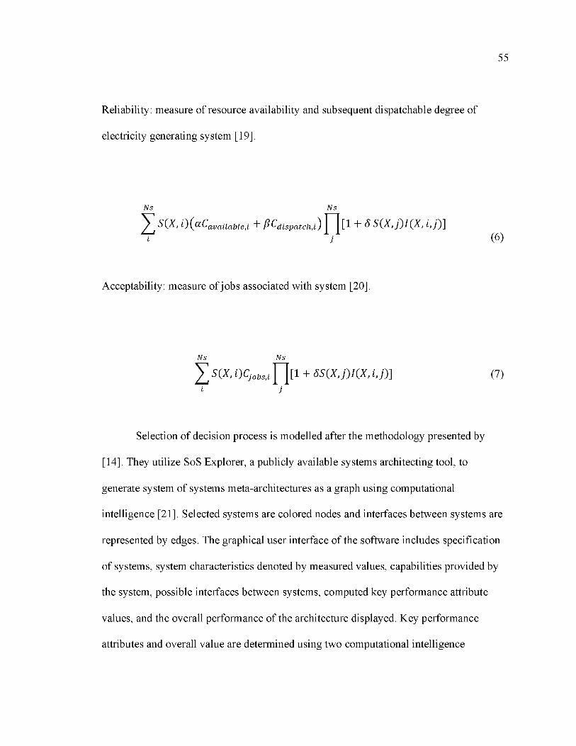
55
Reliability: measure of resource availability and subsequent dispatchable degree of
electricity generating system [19].
Ns Ns
^ S(X , Q ( a C a v a i l a b l e i + pcd i s p a t c h i + S S ( X , j ) I ( X , i , j ) ]
i j (6)
Acceptability: measure of jobs associated with system [20].
Ns Ns
^ S(X , i)Cj o b s i n + 5 S ( X , j ) l ( X , i , j ) ] (7)i j
Selection of decision process is modelled after the methodology presented by
[14]. They utilize SoS Explorer, a publicly available systems architecting tool, to
generate system of systems meta-architectures as a graph using computational
intelligence [21]. Selected systems are colored nodes and interfaces between systems are
represented by edges. The graphical user interface of the software includes specification
of systems, system characteristics denoted by measured values, capabilities provided by
the system, possible interfaces between systems, computed key performance attribute
values, and the overall performance of the architecture displayed. Key performance
attributes and overall value are determined using two computational intelligence

56
techniques that are imbedded within the SoS Explorer Software: fuzzy logic and genetic
algorithm.
Each key performance attribute is represented by a universe of discourse from 0
to 100, where lower values correspond to undesirable performance. A key tenet of fuzzy
logic is the allowance of overlapping membership functions and rules that result in
multiple evaluation scoring regions. This procedure is conducted within MATLAB’s
type-1 Fuzzy Logic toolbox where a fuzzy inference system is created. The membership
function for eco-friendly is presented in Figure 1. A similar function exists for each of the
other KPAs and overall architecture assessment.
Figure 1. Eco-friendly Membership Function
Discrete values for key performance attributes are sent to the fuzzy inference
system to undergo “fuzzifying” in accordance with the membership functions and rules
governed by linguistic relationships (AND or OR) between attributes. These rules are
presented in an IF-THEN format that corresponds to stakeholder input. For example, if
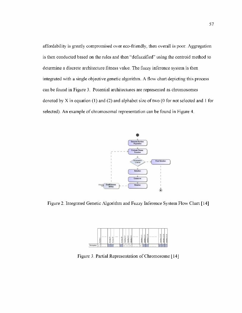
57
affordability is greatly compromised over eco-friendly, then overall is poor. Aggregation
is then conducted based on the rules and then “defuzzified” using the centroid method to
determine a discrete architecture fitness value. The fuzzy inference system is then
integrated with a single objective genetic algorithm. A flow chart depicting this process
can be found in Figure 3. Potential architectures are represented as chromosomes
denoted by X in equation (1) and (2) and alphabet size of two (0 for not selected and 1 for
selected). An example of chromosomal representation can be found in Figure 4.
Figure 2. Integrated Genetic Algorithm and Fuzzy Inference System Flow Chart [14]
Figure 3. Partial Representation of Chromosome [14]

58
4. RESULTS AND DISCUSSION
SoS Explorer uses a single objective genetic algorithm coupled with fuzzy
inference system to generate meta-architecture(s). Note that architecture is plural in that
the potential for multiple architectures can be generated that have different KPA scores,
but the same overall score. The potential solution with the highest overall score was
chosen and will be discussed further in this section. Figure 5 presents the key
performance attribute and overall performance objective values of the selected meta
architecture which is presented graphically in Figure 6. Parameters used for the single
objective genetic algorithm can be found in the upper left-hand corner of Figure 6. The
meta-architecture selected is the result of constituent systems and interfaces selected, key
performance attribute selection, equation formulation, system characteristic values, and
context-specific constraints. Multiple constraints governed the selection of this solution.
First, two independent-of-context constraints were used that ensured feasibility of
potential solutions (i.e. interfaces must be specified if they are to be represented) and
added constituent systems and interfaces so that every identified capability was featured.
Additionally, constraints were developed that ensured upstream and downstream systems
were active (i.e. if a hydropower system is chosen, then the water system must also be
chosen and have an active interface).

59
Figure 4. Key Performance Attribute and Overall Performance Score [21]
Figure 5. Electricity Supply System-of-Systems Meta-Architecture [21]
Performance across the key performance attributes demonstrates the trade space
that exists for this specific use-context. Affordability achieves the highest score, 74.98.
Further, reliability, eco-friendly, and efficiency all achieve scores greater than 50. Lastly,
60
acceptability achieves the lowest score, 48.08. These composite scores aggregate further
to an overall score of 74.56. These trade-offs are the result of the fuzzy inference system
rules selected to represent the complex relationship between each of these attributes. As
mentioned before, colored nodes represent chosen systems and edges represent an
interface between two systems. Several systems and interfaces were not chosen because
they did not add value to the meta-architecture. For example: lignite, subbituminous, and
anthracite (different grades of coal) were not chosen because bituminous represented the
greatest performance across the key performance attributes. The final solution is
potentially representative of future state electricity portfolios. Natural gas and coal-fired
power plants are active systems while Nuclear is not. Most coal-fired power plants are
scheduled for decommissioning in the coming years and others are being converted to
natural gas. Lastly, almost every renewable energy technology was chosen. This is
largely due to the system boundary developed for the problem resulting in certain costs
not being accounted for. In this instance, all power plants were taken “as-built” meaning
the life cycles associated with the construction process is not reflected in model
assessment. However, renewable energy systems are dependent on rare earth elements
that possess complex supply systems that should be captured in future model
development and improvement.

61
5. CONCLUSION
Multi-criteria decision making was identified as a useful approach for handling
the complexity in the energy planning and selection process. A review of commonly cited
multi-criteria decision-making methods in the energy planning literature were reviewed
and determined to be effective for ranking alternatives, but not for determining crisp
values of complete system of systems architectures. To address this gap, computational
intelligence techniques were presented, namely fuzzy logic and genetic algorithms. These
techniques captured the ambiguity among and between key performance attributes and
generated an optimal architecture. The findings presented here consist of a suite of useful
information for energy decision makers and policy professionals. First, the optimal meta
architecture reviewed is potentially representative of future state-level electricity
portfolios: coal, natural gas, hydro, solar, and wind are all present. However, geothermal
is present and nuclear is not. This selection is representative of the shifting trends in
energy portfolio management as nuclear is not often mentioned in future energy scenarios
due to its tenuous relationship with the public. Second, decision makers can manipulate
the systems and interfaces selected to determine how well their portfolio performs in
comparison. Taken together, this methodology provides energy decision makers and
policy professionals with a useful tool and subsequent findings to further inform their
decision making.
Model findings are moderately reflective of actual energy portfolios at the state-
level and deviations from reality can largely be attributed to limitations and addressing

62
them constitutes future work as follows. Characteristic values for constituent systems
were chosen that closely reflect the actual systems but are not based on any specific
literature or governmental documents. Rules that govern the key performance attribute
values were determined in response to the literature but may be changed to better fit a
different context and generate different architectures as a result. Energy systems were
considered post-construction. This distinction is relevant as supply challenges exist for
the rare earth elements that several renewable energy systems depend on. Greenhouse
gases were the only waste generated within the system boundary. Combustion by
products have unique life cycles that if represented would enrich the findings presented
here. Policy disruptions, such as tax breaks or incentives, could be included to help
determine the effects of their implementation. Lastly, time is not directly represented in
the model. A dynamic architecture model could be formulated that captures the
decommissioning of legacy systems and the selection, construction, and operation of
replacements over their respective lifetimes. Addressing these limitations presents ample
potential for future research that will improve the model’s effectiveness and the ability of
energy planners and policy professionals to begin transitioning their energy portfolios
toward a renewable and sustainable future.
ACKNOWLEDGEMENTS
The authors gratefully acknowledge the DOE SUNSHOT GEARED program for
partially funding this research through DOE Project DE-EE0006341

63
REFERENCES
[1] NOAA (2019). Climate Change and Variability | National Centers for Environmental Information (NCEI) formerly known as National Climatic Data Center (NCDC). [online] Ncdc.noaa.gov. Available at:https://www.ncdc.noaa.gov/climate-information/climate-change-and-variability [Accessed 7 Nov. 2019].
[2] United Nations (2019). What is the Paris Agreement? | UNFCCC. [online] Unfccc.int. Available at: https://unfccc.int/process-and-meetings/the-paris- agreement/what-is-the-paris-agreement [Accessed 5 Nov. 2019].
[3] World Bank (2019). [online] Spappssecext.worldbank.org. Available at: http:// spappssecext.worldb ank.org/ sites/indc/Pages/INDCHome.aspx [Accessed 17 Nov. 2019].
[4] AG Energiebilanzen (2019). Germany’s energy consumption and power mix in charts. [online] Clean Energy Wire. Available at:https://www.cleanenergywire.org/factsheets/germanys-energy-consumption-and- power-mix-charts [Accessed 6 Nov. 2019].
[5] EIA (2019). U.S. energy facts explained - consumption and production - U.S. Energy Information Administration (EIA). [online] Eia.gov. Available at: https://www.eia.gov/energyexplained/us-energy-facts/ [Accessed 8 Sep. 2019].
[6] E. Georgopoulou, D. Lalas, L. Papagiannakis, A multicriteria decision aid approach for energy planning problems: The case of renewable energy option, European Journal of Operational Research, vol. 103, pp. 38-54, 1997.
[7] S.D. Pohekar, M. Ramachandran, Application of multi-criteria decision making to sustainable energy planning - a review, Renew. Sustain. Energy Rev. 8 (4) (2004) 365e381.
[8] H. Karunathilake, K. Hewage, W. Merida, R. Sadiq, Renewable energy selection for net-zero communities: Life Cycle based decision making under uncertainty, Renewable Energy, vol. 130, pp. 558-573, June 2019.
[9] J.R. San Cristobal, Multi-criteria decision-making in the selection of a renewable energy project in Spain: the Vikor method, Renew. Energy 36 (2) (Feb. 2011) 498e502.

64
[10] R. Abu Taha, T. Daim, Multi-criteria applications in renewable energy analysis, a literature review, in: T. Daim, T. Oliver, J. Kim (Eds.), Green Energy and Technology vol. 60, Springer London, London, 2013, pp. 17e30.
[11] E. Loken, Use of multicriteria decision analysis methods for energy planning problems, Renew. Sustain. Energy Rev. 11 (7) (Sep. 2007) 1584e1595.
[12] H.-S. Shih, H.-J. Shyur, E.S. Lee, An extension of TOPSIS for group decision making, Math. Comput. Model. 45 (7e8) (Apr. 2007) 801e813.
[13] T. Daim, T. Oliver, J. Kim, Research and Technology Management in the Electricity Industry, vol. 60, Springer London, London, 2013.
[14] L. Ashiku, C. Dagli, System of Systems (SoS) Architecture for Digital Manufacturing Cybersecurity, 25th International Conference on Production Research Manufacturing Innovation: Cyber Physical Manufacturing, 00, 2019.
[15] H. C. Doukas, B. M. Andreas, J. E. Psarras, Multi-criteria decision aid for the formulation of sustainable technological energy priotirties using linguistic variables, European Journal of Operational Research, vol. 182, pp. 844-855, 2006.
[16] K. Gulzar, J. Sang, M. Ramzan, M. Kashif, Fuzzy approach to prioritize usability requirements conflicts: An experimental evaluation, IEEE, vol. 5, pp. 1357013577, 2017.
[17] B. Atilgan, A. Azapagic, An integrated life cycle sustainability assessment of electricity generation in Turkey, Energy Policy, vol. 93, pp. 168-186, 2016.
[18] L. Pape, K. Giammarco, J. Colombi, D. Dagli, N. Kilicay-Ergin, A fuzzy evaluation method for system of systems meta-architectures, Procedia Computer Science, vol. 16, pp. 245-254, 2013.
[19] DOE (2017). [online] Energy.gov. Available at: https://www.energy.gov/sites/prod/files/2017/01/f34/Chapter%20IV%20Ensuring %20Electricity%20System%20Reliability%2C%20Security%2C%20and%20Resi lience.pdf [Accessed 8 Oct. 2019].
[20] M. Bojesen, L. Boerboom, H. Skov-Petersen, Towards a sustainable cpaacity expansion of the Danis hbiogas sector, Land Use Policy, vol. 42, pp. 264-277, 2015.
[21] Missouri S&T (n.d.). SOS Explorer - Engineering Management and Systems Engineering | Missouri S&T. [online] Emse.mst.edu. Available at: https://emse.mst.edu/sos-explorer/ [Accessed 16 Sep. 2019].
65
IV. A TIME SERIES SUSTAINABILITY ASSESSMENT OF A PARTIAL ENERGY PORTFOLIO TRANSITION
Jacob Hale and Suzanna Long
Department of Engineering Management and Systems Engineering, Missouri University of Science and Technology, Rolla, MO 65409
ABSTRACT
Energy portfolios are overwhelmingly dependent on fossil fuel resources that
perpetuate the consequences associated with climate change. Therefore, it is imperative
to transition to more renewable alternatives to limit further harm to the environment. This
study presents a univariate time series prediction model that evaluates sustainability
outcomes of partial energy transitions. Future electricity generation at the state-level is
predicted using exponential smoothing and autoregressive integrated moving average
(ARIMA). The best prediction results are then used as an input for a sustainability
assessment of a proposed transition by calculating carbon, water, land, and cost
footprints. Missouri, USA was selected as a model testbed due to its dependence on coal.
Of the time series methods, ARIMA exhibited the best performance and was used to
predict annual electricity generation over a 10-year period. The proposed transition
consisted of a one-percent annual decrease of coal’s portfolio share to be replaced with an
equal share of solar and wind supply. The sustainability outcomes of the transition
demonstrate decreases in carbon and water footprints but increases in land and cost

66
footprints. Decision makers can use the results presented here to better inform strategic
provisioning of critical resources in the context of proposed energy transitions.
1. INTRODUCTION
Fossil fuel resources provide most of the world’s energy and subsequent carbon
dioxide emissions [1,2]. In 1990, fossil fuels made up more than eighty-six percent of the
total primary energy supply of the United States and its combustion resulted in more than
four thousand eight hundred megatons of carbon dioxide emissions. By 2015, energy
demands increased by almost an additional thirteen percent with carbon dioxide
emissions increasing by more than an additional two and a half percent. During this time,
renewables increased by less than two percent. When excluding biofuels and waste-to-
energy sources, this increase is less than one percent. These findings demonstrate that
portfolios are shifting, but not toward renewables resulting in an increase in already high
carbon dioxide emissions. If this trend continues, the consequences associated with
climate change will be further exacerbated [3]. To minimize further harm to the
environment, fossil fuel dependent energy portfolios, especially those relying on coal,
must be transitioned to renewable alternatives.
Modern energy transitions are defined by a timely shift toward energy systems
that address global energy challenges [4]. Transitions have received widespread scholarly
attention from several perspectives such as socio-technical [5-8], existing system
considerations [9-11], and environmental reform and governance [12-14], among others.
67
An effective approach in quantitative studies is the use of time series forecasting methods
to inform transition decision making. Energy forecasts primarily consist of three temporal
horizons: short-, medium-, and long-term [15]. Short-term forecasts encompass studies
from an hour to a week [16,17]. Medium-term forecasts include a month to five years
[18-20]. Long-term forecasts cover periods from five to 20 years [21-23]. Forecasting is
a data-driven method that relies on statistical procedures to derive relationships between
variables [24]. Standard data-driven forecasting models include moving and weighted-
moving average, simple exponential smoothing, Holt’s Model, and Damped Holt’s
Model [25]. More advanced methods include autoregressive moving average (ARMA)
[26,27], autoregressive integrated moving average (ARIMA) [28,29], and artificial neural
networks [30]. A commonality among these models is the ability to monitor change in
variables between time steps. This is a useful feature for decision makers as it provides
time-dependent information regarding the prediction variable and other performance
characteristics.
This research extends the conventional assessment of energy transitions by
providing a univariate time series prediction of annual electricity generation that monitors
changes in life cycle sustainability performance using a footprint approach. This research
addresses a gap in the literature with respect to standard analysis methods. Standard
comparative analysis currently consists only of weighing cost against emission reductions
over the life cycle of energy sources [31]. The work presented in this research addresses
the gap by conducting an evaluation that provides a more thorough determination of the
relationship between energy source selection and sustainability impact using a footprint

68
approach [32]. A footprint approach can be conducted by accounting for carbon (g
CO2/kWh), water (m3/kWh), land (m2/kWh), and levelized cost (cents/kWh) over the
duration of the energy source life cycle in a time series transition context.
Missouri was selected as a model test bed to demonstrate methodological efficacy
due to the state’s dependency on coal. The proposed model is a data-driven approach that
uses annual state-level electricity portfolio data from 2001 to 2019 to build a time series
prediction of electricity generation. This prediction is then used as an input for a
sustainability assessment that monitors metric performance of a proposed transition. The
scenario presented consists of a decrease of coal’s portfolio share that is subsequently
replaced by renewable alternatives, solar and wind. By including life cycle measurements
of sustainability performance, energy decision makers are providing socially responsible
stewardship of transition outcomes. Further, these outcomes evaluate a proposed
transition in the context of natural resource consumption and emissions production.
Energy decision makers can use these results to better guide allocation of resources and
to align energy transition strategies with sustainability goals beyond the "do no harm"
threshold [33]. The following section presents the data used, time series methods applied,
and mechanics of the energy transition.

69
2. MATERIALS AND METHODS
2.1. DATA
Historical data is required to produce a time series prediction. The Energy
Information Administration (EIA) maintains annual and monthly state-level energy
portfolio data. Figure 1 displays annual electricity generation for Missouri from 2001 to
2019 [34]. There are two features of the data that determinate the selection of an
appropriate forecasting method. First, the data does not exhibit trend or seasonality. This
eliminates methods such as Holt’s Model, Holt-Winter’s Model, and variations therein
from consideration. Second, the sample size is small consisting of nineteen data points.
Small sample sizes limit the application of more sophisticated methods that generally
return results that are more accurate. However, exponential smoothing [35,36] and
autoregressive integrated moving average (ARIMA) [37,38] are two effective approaches
for generating time series predictions for energy datasets given these constraints. Table 1
provides sustainability indicator values converted to kW-hr to be consistent with the time
series prediction [32].
2.2. TIME SERIES PREDICTION OF ELECTRICITY GENERATION
Using historical data, a univariate time series prediction of annual electricity
generation for Missouri was created. The Forecast Library in r was used to fit exponential
smoothing and ARIMA models to the data [39]. Exponential smoothing models can be
classified using a three-letter convention [40]. The letters denote error type, trend, and

70
seasonality, respectively. There are three options for each of the cases: N (none), A
(additive), and M (multiplicative). Similarly, ARIMA also follows a three-letter scheme.
The nomenclature refers to autoregressive terms, non-seasonal differences required for
stationarity, and lagged forecast errors in the prediction equation. In this instance, the
exponential smoothing (A, N, N) and ARIMA models (1, 0, 0) were selected. This class
of exponential smoothing is often referred to as the simple version.
Annual Electricity Generation, Missouri (2001-2019)
100,000 ----------------------------------------------------------------------------------
70,000
2001
2002 no
8rsj 20
0420
0520
0620
07 00
8rsj 20
0920
1020
1120
12 noi
Orsj 20
1420
1520
1620
17 00 T—11orsj
Year
Figure 1. Total Electricity Generation, Missouri 2001-2019

71
Table 1. Sustainability Indicators of Various Energy Types
E n e rg y T y p eC a rb o n F o o tp r in t
(g C O 2/k W h )W a te r F o o tp r in t
(m 3/k W h )L a n d F o o tp r in t
(m 2/k W h )C o s t
(c e n ts /k W h )
C o a l 8.34 x 10² - 1.03 x 10³ 5.40 x 10⁻⁴ - 2.09 x 10⁻³ 8.3 x 10⁻⁵ - 5.7 x 10⁻⁴ 3.77-5.85
S o la r
P h o to v o l ta ic1.25 x 101 - 1.04 x 10² 1.51 x 10⁻⁴ 7.04 x 10⁻⁴ - 1.76 x 10⁻³
1.09 x 1012.34 x 101
W in d :o n s h o r e
6.90 - 1.45 x 101 3.60 x 10⁻⁶ 2.17 x 10⁻³ - 2.64 x 10⁻³ 4.16-5.72
Simple exponential smoothing uses a smoothing constant, alpha, to attach a
unique weight to each observation where weights decrease exponentially the further the
data reference point is from the prediction. A smoothing constant of one was selected
using the simplex method by minimizing the Corrected Akaike Information Criterion
(AICc) which is presented later. This criterion is also used to select the ARIMA model.
The component form of simple exponential Energies 2021, 14, 141 4 of 14 smoothing is
given in Equations (1) and (2) [25]. Equation (1) presents the level forecast and Equation
(2) provides the smoothing procedure.
yT+h — Yt
It — ayt + (1 - a)!t- i
(1)
(2)
s.t. 0 < a < 1

72
Mathematical notation for ARIMA models is provided in Equation (3) [25]. The
class of ARIMA model that minimized AICc is referred to as the first-order
autoregressive model or ARIMA (1, 0, 0). In this case, predictions are calculated as a
function of the previous value, slope coefficient phi, and constant mu. Slope coefficient
and constant terms are provided in Table 2. It can be observed that the autoregressive
term is 0.7932 and the constant term is 84,508. Theta corresponds to the moving average
portion of the model. For this class of ARIMA models, there is no moving average
component, and therefore it is not provided.
(1 - - • 0 pf l P ) ( l - B) d y t = c + ( l + 0 1B + - 0 q B^)e t (3)
Where,
B = backshift operator,
c = K i - 0 i - --0 p) ,
p = ( i - B)d y t
Equations for AIC and AICc for ARIMA models are provided in Equations (4)
and (5) [25]. Similar equations for exponential triple smoothing models can be found at
the accompanying reference. L is the likelihood of the data and k is a binary variable that
equals one if there is an intercept. AICc is a modified version of AIC that provides a bias
correction for smaller datasets as it corrects for the sample size with T.

73
Table 2. ARIMA (1,0,0) COEFFICIENTS
0 p
ARIMA
(1,0,0) 0.7932 84,508
Standard
Error 0.1547 3,802
A I C = - 2 L o g ( L ) + 2(p + q + k + 1) (4)
2(p + a + k + l ) (p + q + k + 2 )A I C c = A I C + — — \ 7 ^----------
c T - p - q - k - 2(5)
The method with the best performance across these summary statistics is selected as the
input for the sustainability assessment.
2.3. MECHANICS OF ENERGY TRANSITION
Equation 6 demonstrates how the total electricity generation prediction (Elt) is
partitioned into fulfillment by a given electricity source. A coefficient (X) corresponds to
the most recently reported portfolio share for that electricity source.

74
E l i — X i E l t (6)
W here X represents initial portfolio share for electricity source i
The proposed transition will consist of decreasing coal’s portfolio share (Elc) and
replacing it with a mix of wind (Elw) and solar energy (Els). Equations 7-9 provide
transition mechanics. A proportional rate of change is provided to determine allocation of
newly available portfolio between solar and wind.
E l c — E l c 0 - r t E l t (7)
W here r = annual rate of change,
t = time
E l s — E l s ,o + y r t E l t (8)
W here y = proportional rate of change applied
E l w — E l w 0 + ( 1 - y ) r t E l t (9)
Sustainability of a proposed transition can be summarized by equation 10. A
given energy source’s portfolio share is first determined using equation 6. Next, the
electricity provided by a given source is then multiplied by the corresponding
sustainability indicator value. A summation of each of these product operations is then
conducted to determine the specific footprint value. The following section provides
results generated using this methodology.

75
3F t = ^ F g ,i E l i
i =1
Where t = footprint type, g = footprint rate associated with energy source i
(10)
3. RESULTS
This research consists of three contributions: (1) Development and Comparison of
Time Series Forecasting Methods, (2) Sustainability Evaluation of Proposed Electricity
Portfolio Transition, and (3) Comparison of Different Fulfillment Strategies. Time series
forecasting methods possess inherent uncertainty and measures therein are provided when
appropriate.
3.1. DEVELOPMENT AND COMPARISON OF TIME SERIES FORECASTING METHODS
Using the Forecast Library in r, simple exponential smoothing and ARIMA
models were fit to the annual state-level electricity generation dataset. The results of this
procedure are presented graphically in Figure 2. Actual data is denoted in blue, simple
exponential smoothing in orange, and ARIMA in grey. ETS stands for exponential triple
smoothing of which simple exponential smoothing is a variant. It can be observed that the
simple exponential smoothing forecast selects the most recent observation as the
prediction for the current time step. The ARIMA model is governed by different

76
equations, but ultimately yields similar results. However, superior performance is
difficult to determine upon visual inspection alone.
AICc values for each of the models are presented in Table 3. A smaller value
corresponds to a model that is better fit to the data. The ARIMA model slightly
outperforms simple exponential smoothing for this dataset. Additional assessment is
required before the optimal model can be determined.
Forecasting Model Comparison
70,000r - i r \ i m ' 3 - L n c o r ' - o o c n o r - i r \ i m ' 3 - L n c oO O O O O O O O O t H t H t H t H t H t - l t - lo o o o o o o o o o o o o o o o
N 00 Olo o o
•Actual Data
Year
■ Forecast (ETS) •Forecast (ARIMA)
Figure 2. Forecasting Model Comparison
100.000
An alternative approach that augments visual inspection and summary statistical
analysis is the evaluation of prediction intervals for each of the models. Figure 3
illustrates a 10-year prediction using each of the models. One shortcoming of simple

77
exponential smoothing is that the prediction is given as a ‘flat’ value. This behavior is
unlikely to be representative of future energy generation scenarios. Alternatively, the
ARIMA model trends upward before flattening out. Figures 4 and 5 investigate the 95%
prediction interval for simple exponential smoothing and ARIMA, respectively. In Figure
4, the prediction interval continuously expands as the forecast horizon increases. The
prediction interval width at the final forecasted value is almost 50,000 (thousand MWh).
Alternatively, ARIMA’s prediction interval provided in Figure 5 provides is greater than
24,000 (thousand MWh). This represents a significant reduction in uncertainty when
compared to the simple exponential smoothing model.
Table 3. AICc for Time Series Prediction Models
Model AICc
ETS (A,N,N) 375.56
ARIMA
(1,0,0) 373.64

78
Forecasting Model Comparison with Predictions100,000 ----------------------------------------------------------------------------------------------------
70,000 ---------------------------------------------------------------------------------------------------------x H r O L n r ^ c n ^ H r O L n r ^ c n ^ H r O L n r ^
8 8 8 8 8 0 0 0 0 0 8 8 8 8r \ i r \ i r \ i r \ i r \ i r \ i r \ i r \ i r \ i r \ i r \ i r \ i r \ i c \ i
Year
^ ^ “ Actual Data Forecast (ETS) Forecast (ARIMA)
Figure 3. Forecasting Model Comparison with Predictions
Actual Data vs. ETS with 95% Prediction Intervalg 110,000 -------------------------------------------------------------------------------------------------
LU
40,000
2001
2003
2005
2007
2009
2011
2013
2015
2017
2019
2021
2023
2025
2027
2029
Year
Actual Data Forecast (ETS)
. . Lower 95% PI (ETS)
Figure 4. Actual Data vs. ETS with 95% Prediction Interval
2029
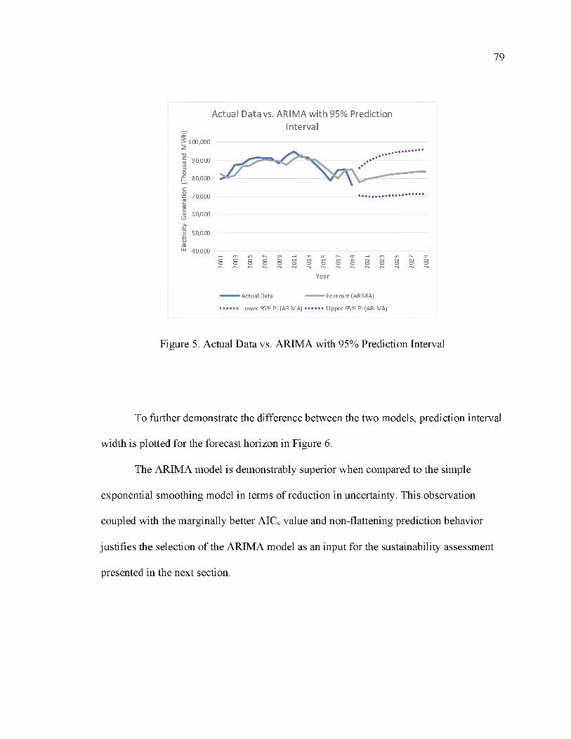
79
Actual Data vs. ARIMA with 95% Prediction Interval
<1)
60,000
50,000 ------------------------------------------------------------------------------------------------------------tj_cy
m 40,000 ------------------------------------------------------------------------------------------------------------r H m L n h ' C n ^ H m L n h ' C n ^ H m L n h ' C n
8 Q Q Q Q , h , h , h , h , h ^ ^ ^ ^ ^ O O O O O O O O O O O O O OC ' l C ' i C ' i C ' i C ' i C ' i C ' i C ' i C ' i C ' i C ' i C ' i C ' i C ' i C ' i
Year
Actual Data Forecast (ARIMA)
.......... Lower 95% PI (ARIMA).............Upper 95% PI (ARIMA)
Figure 5. Actual Data vs. ARIMA with 95% Prediction Interval
To further demonstrate the difference between the two models, prediction interval
width is plotted for the forecast horizon in Figure 6.
The ARIMA model is demonstrably superior when compared to the simple
exponential smoothing model in terms of reduction in uncertainty. This observation
coupled with the marginally better AICc value and non-flattening prediction behavior
justifies the selection of the ARIMA model as an input for the sustainability assessment
presented in the next section.

80
95% Prediction Interval Comparison60,000
50,000
40,000
30,000
20,000
10,000
Year
Upper 95% PI - Lower 95% PI (ETS) Upper 95% PI - Lower 95% PI (ARIMA)
0
Figure 6. 95% Prediction Interval Width Comparison
3.2. SUSTAINABILITY ASSESSMENT OF PROPOSED ELECTRICITY PORTFOLIO TRANSITION
Fitting a time series model to volatile data is a complex task. This is demonstrated
by the summary statistic performance of both models and the uncertainty present denoted
by the prediction interval widths. Initial electricity source portfolio shares are provided in
Table 4. Sustainability assessment results are given for both prediction intervals and
model predictions in Table 5.
The 10-year percentage change for each of the footprints is provided in a min-
max format. This is due to the data being provided in range format. Minimum values
correspond to best-case performance for each of the footprint categories. Alternatively,
maximum values provide a worst-case scenario. The upper 95 percent prediction interval

81
scenario reflects a substantive increase in electricity from 2020 to 2029. This increase in
electricity generation offsets the sustainability improvements where only carbon footprint
is reduced in both minimum and maximum cases. Except for water’s maximum case,
each of the other footprints increases in this scenario. For the ARIMA prediction, carbon
and water footprints decrease. Land and cost footprints increase significantly. This is due
to the higher values reported for the renewable technologies. The best performance is
achieved for the lower 95% prediction interval. As electricity generation is decreased, the
sustainability improvement will be more pronounced. Similarly, to the ARIMA
prediction performance, carbon and water decrease while land and cost increase.
However, each of the footprints is decreased considerably from the model’s prediction.
This finding suggests that the best sustainability performance will be achieved in the
event that electricity generation decreases and a transition to renewable alternatives is
conducted in a timely manner.
Table 4. Initial Model Configuration
Electricity Initial Portfolio Share
Source (Xi)
Coal 72.82%
Wind 3.76%
Solar 0.52%
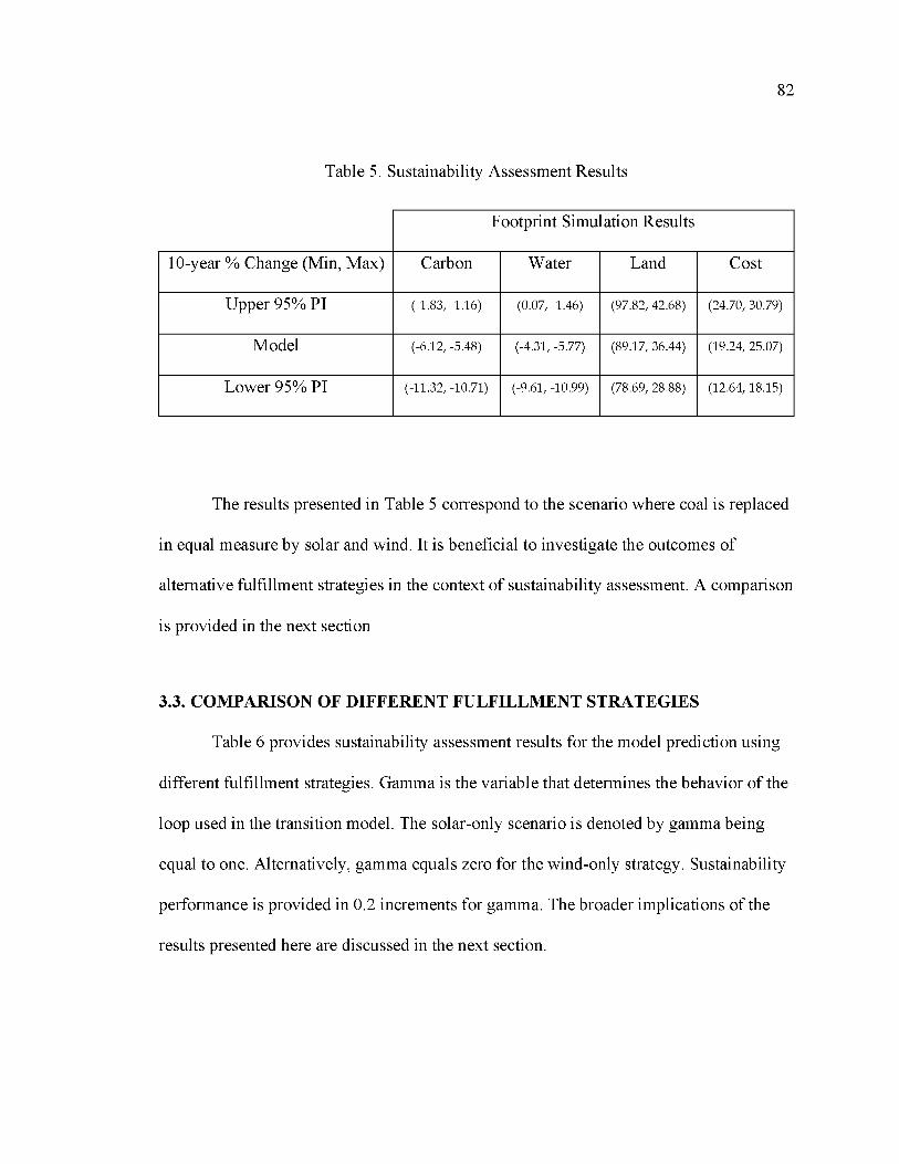
82
Table 5. Sustainability Assessment Results
Footprint Simulation Results
10-year % Change (Min, Max) Carbon Water Land Cost
Upper 95% PI (-1.83, -1.16) (0.07, -1.46) (97.82, 42.68) (24.70, 30.79)
Model (-6.12, -5.48) (-4.31, -5.77) (89.17, 36.44) (19.24, 25.07)
Lower 95% PI (-11.32, -10.71) (-9.61, -10.99) (78.69, 28.88) (12.64, 18.15)
The results presented in Table 5 correspond to the scenario where coal is replaced
in equal measure by solar and wind. It is beneficial to investigate the outcomes of
alternative fulfillment strategies in the context of sustainability assessment. A comparison
is provided in the next section
3.3. COMPARISON OF DIFFERENT FULFILLMENT STRATEGIES
Table 6 provides sustainability assessment results for the model prediction using
different fulfillment strategies. Gamma is the variable that determines the behavior of the
loop used in the transition model. The solar-only scenario is denoted by gamma being
equal to one. Alternatively, gamma equals zero for the wind-only strategy. Sustainability
performance is provided in 0.2 increments for gamma. The broader implications of the
results presented here are discussed in the next section.

83
Table 6. Sustainability Evaluation for Different Fulfillment Strategies
C a r b o n F o o tp r in t W a te r F o o tp r in t
L a n d
F o o tp r in t
C o s t
F o o tp r in t
Y M in M a x M in M a x M in M a x M in M a x
1
(so la r -o n ly )-6.07% -4.89% -2.46% -5.29% 46.61% 28.72% 29.84% 42.60%
0.8 -6.09% -5.12% -3.20% -5.48% 64.11% 31.82% 25.63% 35.67%
0.6 -6.11% -5.36% -3.94% -5.68% 80.97% 34.90% 21.38% 28.63%
0.5 -6.12% -5.48% -4.31% -5.77% 89.17% 36.44% 19.24% 25.07%
0 .4 -6.13% -5.60% -4.68% -5.87% 97.21% 37.97% 17.10% 21.49%
0.2 -6.15% -5.84% -5.42% -6.06% 112.87% 41.01% 12.77% 14.24%
0
(w in d -o n ly )-6.16% -6.07% -6.16% -6.25% 127.98% 44.03% 8.41% 6.87%
4. DISCUSSION
Two time series prediction methods, ARIMA and exponential smoothing, were
used to develop a prediction of Missouri’s annual electricity generation. ARIMA
exhibited superior performance measured across key summary statistics. Given these
findings, a 10-year prediction of electricity generation was generated. The result of this
procedure was used as an input for the sustainability assessment model. Initial portfolio

84
share values for coal, solar, and wind were determined and used for model initialization.
Coal’s initial share (72.82%) was decreased at a rate of one percent per year. Therefore,
at the end of the simulation coal accounted for ten percent less of the portfolio. Solar
(0.52%) and wind (3.76%) accounted for this decrease in portfolio share in equal
measure. A ten-percent decrease in coal’s portfolio share resulted in a carbon footprint
decrease (-6.12, -5.48) and water footprint decrease (-4.31, -5.77). Alternatively, land
footprint increased (89.17, 36.44) and levelized cost increased (19.24, 25.07). Note that
change in footprint is presented as a range of percentages instead of a discrete value. This
is due to the literature reporting the values as a range derived from longitudinal studies.
As reported in Table 1, some energy sources possess a larger range of values for a given
indicator. Table 5 was generated to demonstrate the proposed transition’s sensitivity to
both the range of sustainability values used and the uncertainty inherent in the model
prediction. Except for water footprint, each of the energy sources exhibit a range of
values for each of the energy sources considered. Coal possesses a larger carbon and
water footprint. However, coal has the smallest land footprint and a comparably low-cost
footprint. The magnitude of these differences is best understood in the context of
scenarios presented in Table 5. The upper prediction interval demonstrated marginal
improvement in carbon and water footprints and large increases to both land and cost
footprints. This can be attributed to the increase in generation required not effectively
offsetting coal’s decreased portfolio share. It can be observed that as electricity
generation decreased, sustainability outcomes improved. As less energy is generated, the
gains from decreasing coal’s portfolio share will be more pronounced. Less electricity is

85
generated in this case and more of it is being fulfilled by renewable sources. Therefore,
the lowest prediction interval returns the best sustainability performance. For this
research, an equal share of newly available portfolio was allocated to both wind and
solar. Table 6 provides simulation results for different fulfillment strategies using the
model prediction. The wind-only strategy achieves the best results for carbon, water, and
cost footprints. Land footprint, however, is much larger and represents the worst
performance. Alternatively, solar outperforms wind in land footprint performance alone.
Intermediate gamma values demonstrate that sustainability performance improves as
gamma is decreased. However, an optimal gamma value is not presented here as it is
subject to derivation of a weighting scheme for each of the indicators consistent with
stakeholder input. The sustainability assessment results presented here underscore a few
key considerations for energy decision makers tasked with transitioning current
fulfillment strategies. First, a transition to existing renewable energy alternatives is not a
panacea for climate change mitigation. Where renewables demonstrate positive
performance in carbon and water footprint results, they perform negatively for land and
cost. This is important to capture as sustainability involves more than just the relationship
between carbon emissions and cost. Second, the impact of the sustainability performance
presented here is not confined to the state of Missouri. Energy supply systems for both
fossil fuel and renewable sources are national, and in some cases, global. Therefore, local
energy decision making has global consequences. Lastly, the lower ninety-five percent
prediction interval exhibited the best sustainability performance. This finding
demonstrates the effectiveness of a strategy that couples a transition to renewables and
86
improvements in technological efficiency that reduce electricity generation. These
findings are subject to some limitations that provide ample room for future research. The
time series model predicts upward trending behavior that eventually flattens. Future
values are unlikely to exhibit this behavior given the volatility of the historical data.
Exploration of other prediction methods and use of higher resolution temporal data might
generate more accurate and dependable results. Selection of an optimal gamma value
should be determined with input from key stakeholders. This can be accomplished
through the implementation of a Delphi Method and subsequent analysis. A similar
stakeholder engagement procedure could also be followed to determine which scenario
presented in Table 6 is chosen. If either of the upper intervals are used, then the outcome
could be an increase in the net export of electricity or idle capacity installed.
Alternatively, if the lower intervals are used then importing electricity might be required.
The sustainability assessment model can be converted into a system dynamics model by
incorporating additional feedback loops. At present, the rate of change constitutes the
only feedback mechanism in the model. Candidate feedback loops include different
policy effects, relationships between sustainability indicators, and response to system
disruptions, among others. Further, the holistic sustainability approach could be extended
to account for other metrics such as dispatchability, resilience, and job creation. The
range of footprint values can be further specified by deploying state-specific data
gathering efforts. If accomplished, the variability of findings would be decreased
resulting in an improved model. Additionally, evaluation of other renewable energy
technologies including distributed energy resources should be conducted. This would
87
include the analysis of alternative energy mix scenarios subject to data availability. Solar
and wind power were selected here given their comparably large share of Missouri’s
renewable electricity portfolio. Lastly, an optimal implementation plan should be
provided given a proposed energy transition. In the following section, a summary of the
research is provided with concluding remarks.
5. CONCLUSION
Global energy portfolios are dependent on fossil fuel resources. This dependence
results in the continuous emission of greenhouse gases that harm the environment.
Beyond these concerns, energy sources also have an impact on other natural resources
such as land and water. Therefore, energy decision makers must transition current
portfolios to renewable alternatives while monitoring unintended sustainability impacts.
The model presented provides a univariate time series prediction of annual electricity
generation using publicly available data. The method exhibiting the best performance,
ARIMA, was then used as an input for the sustainability assessment model that monitors
the performance of a proposed transition using a footprint approach. Using Missouri as a
testbed, coal’s share of the portfolio was decreased by one percent annually and replaced
with an equal share of wind and solar power over a ten-year period. Model findings
demonstrate that such a transition would decrease carbon and water footprints while
increasing land and cost footprints. However, the prediction intervals underscore the
range of sustainability outcomes. The best performance occurs if annual electricity

88
generation decreases. This finding affects several aspects of management and
governance. Energy decision makers can change fulfillment strategies, but not antecedent
demand behavior. Electricity and, more broadly, energy serve a crucial role in industrial
processes. Therefore, sustainability performance like the approach provided here should
guide product design and supply chain configuration. Practitioners can use these results
to prioritize the sustainable procurement of raw materials through to more preferred end-
of-life management techniques such as reuse [41]. Additionally, research and
development efforts should design product architectures with improved efficiency.
Governments can encourage such behavior through policy incentivization. Subsequently,
energy use, and thus demand for electricity generation would decrease resulting in
improved sustainability performance. Various decision makers are engaged in energy
transitions and sustainability improvements. Policy professionals are tasked with passing
laws that encourage the adoption of renewable energy technologies. Business entities
should bring products to market that perform well on sustainability measures beyond
profit. Lastly, energy decision makers must rapidly transition energy portfolios to
renewable alternatives to limit further harm to the environment. The results presented
here provide decision makers with a quantitative guide to evaluate the sustainability of
proposed energy transition strategies more thoroughly.

89
ACKNOWLEDGEMENTS
The authors gratefully acknowledge the DOE SUNSHOT GEARED program for
partially funding this research through DOE Project DE-EE0006341.
REFERENCES
[1] International Energy Agency, Total Primary Energy Supply (TPES) by Source, World 1990-2017. Available online: https://www.iea.org/data-and- statistics?country=WORLD&fuel=Energy%20supply&indicator=Total%20primar y%20energy%20supply%20(TPES)%20by%20source (accessed on 1 August 2020).
[2] International Energy Agency, CO2 Emissions by Energy Source, World 19902017. Available online: https://www.iea.org/data-and-statistics?country=WORLD&fuel=CO2%20emissions&indicator=CO2%20emissi ons%20by%20energy%20source (accessed on 1 August 2020).
[3] National Aeronautics and Space Administration, The Effects of Climate Change. Available online: https://climate.nasa.gov/effects/ (accessed on 1 June 2020).
[4] Singh, H. V., Bocca, R., Gomez, P., Dahlke, S., & Bazilian, M. (2019). The energy transitions index: An analytic framework for understanding the evolving global energy system. Energy Strategy Reviews, 26(July), 100382.
[5] Meadowcroft, J. (2009). What about the politics? Sustainable development, transition management, and long term energy transitions. Policy Sciences, 42(4), 323-340. https://doi.org/10.1007/s11077-009-9097-z
[6] Verbong, G., & Geels, F. (2007). The ongoing energy transition: Lessons from a socio-technical, multi-level analysis of the Dutch electricity system (1960-2004). Energy Policy, 35(2), 1025-1037. https://doi.org/10.1016/j.enpol.2006.02.010
[7] Kern, F., & Smith, A. (2008). Restructuring energy systems for sustainability? Energy transition policy in the Netherlands. Energy Policy, 36(11), 4093-4103. https://doi.org/10.1016/j.enpol.2008.06.018

90
[8] Rutherford, J., & Coutard, O. (2014). Urban Energy Transitions: Places,Processes and Politics of Socio-technical Change. Urban Studies, 51(7), 1353— 1377. https://doi.org/10.1177/0042098013500090
[9] Tagliapietra, S., Zachmann, G., Edenhofer, O., Glachant, J. M., Linares, P., & Loeschel, A. (2019). The European union energy transition: Key priorities for the next five years. Energy Policy, 132(March), 950-954. https://doi.org/10.1016/j.enpol.2019.06.060
[10] Holsgens, R., Lubke, S., & HasselkuB, M. (2018). Social innovations in the German energy transition: an attempt to use the heuristics of the multi-level perspective of transitions to analyze the diffusion process of social innovations. Energy, Sustainability and Society, 8(1). https://doi.org/10.1186/s13705-018- 0150-7
[11] Schilling, T., Wyss, R., & Binder, C. R. (2018). The resilience of sustainability transitions. Sustainability (Switzerland), 10(12). https://doi.org/10.3390/su10124593
[12] Busch, H., & McCormick, K. (2014). Local power: Exploring the motivations of mayors and key success factors for local municipalities to go 100% renewable energy. Energy, Sustainability and Society, 4(1), 1-15. https://doi.org/10.1186/2192-0567-4-5
[13] Cowell, R. (2017). Sub-national government and pathways to sustainable energy. Environment and Planning. C, Politics and Space, 35(7), 1139-1155.
[14] Parkins, J., Beckley, T., Comeau, L., Stedman, R., Rollins, C., & Kessler, A. (2017). Can Distrust Enhance Public Engagement? Insights From a National Survey on Energy Issues in Canada. Society & Natural Resources, 30(8), 934948.
[15] Sanchez-Duran, R., Luque, J., & Barbancho, J. (2019). Long-term demand forecasting in a scenario of energy transition. Energies, 12(16), 1-24. https://doi.org/10.3390/en12163095
[16] Boroojeni, K. G., Amini, M. H., Bahrami, S., Iyengar, S. S., Sarwat, A. I., & Karabasoglu, O. (2017). A novel multi-time-scale modeling for electric power demand forecasting: From short-term to medium-term horizon. Electric Power Systems Research, 142, 58-73. https://doi.org/10.1016Zj.epsr.2016.08.031
[17] Ryu, S., Noh, J., & Kim, H. (2017). Deep neural network based demand side short term load forecasting. Energies, 10(1), 1-21. https://doi.org/10.3390/en10010003

91
[18] Croonenbroeck, C., & Ambach, D. (2015). A selection of time series models for short- to medium-term wind power forecasting. Journal of Wind Engineering and Industrial Aerodynamics, 136, 201-210. https://doi.org/10.1016/jjweia.2014.11.014
[19] Le, T., Vo, M. T., Vo, B., Hwang, E., Rho, S., & Baik, S. W. (2019). Improving Electric Energy Consumption Prediction Using CNN and Bi-LSTM. Applied Sciences, 9(4237).
[20] Bernardi, M., Petrella, L. Multiple season cycles forecasting model: the Italian electricity demand. Stat Methods Appl 24, 671-695 (2015). https://doi.org/10.1007/s10260-015-0313-z.
[21] Pfenninger, S., & Staffell, I. (2016). Long-term patterns of European PV output using 30 years of validated hourly reanalysis and satellite data. Energy, 114, 1251-1265. https://doi.org/10.1016Zj.energy.2016.08.060
[22] Rahman, A., Srikumar, V., & Smith, A. D. (2018). Predicting electricity consumption for commercial and residential buildings using deep recurrent neural networks. Applied Energy, 212(December 2017), 372-385. https://doi.org/10.10167j.apenergy.2017.12.051
[23] de Oliveira, E. M., & Cyrino Oliveira, F. L. (2018). Forecasting mid-long term electric energy consumption through bagging ARIMA and exponential smoothing methods. Energy, 144, 776-788. https://doi.org/10.1016/j.energy.2017.12.049
[24] Amasyali, K., & El-Gohary, N. M. (2018). A review of data-driven building energy consumption prediction studies. Renewable and Sustainable Energy Reviews, 81(April 2017), 1192-1205. https://doi.org/10.1016/j.rser.2017.04.095
[25] Hyndman, R.J., & Athanasopoulos, G. (2018) Forecasting: principles and practice, 2nd edition, OTexts: Melbourne, Australia. Available online: OTexts.com/fpp2. (Accessed on 7 June 2020)
[26] Alabdulwahab, A., Abusorrah, A., Zhang, X., & Shahidehpour, M. (2015). Coordination of Interdependent Natural Gas and Electricity Infrastructures for Firming the Variability of Wind Energy in Stochastic Day-Ahead Scheduling. IEEE Transactions on Sustainable Energy, 6(2), 606-615. https://doi.org/10.1109/TSTE.2015.2399855
[27] Yang, Z., Ce, L., & Lian, L. (2017). Electricity price forecasting by a hybrid model, combining wavelet transform, ARMA and kernel-based extreme learning machine methods. Applied Energy, 190, 291-305. https://doi.org/10.1016/j.apenergy.2016.12.130
92
[28] Amini, M. H., Kargarian, A., & Karabasoglu, O. (2016). ARIMA-based decoupled time series forecasting of electric vehicle charging demand for stochastic power system operation. Electric Power Systems Research, 140, 378390. https://doi.org/10.10167j.epsr.2016.06.003
[29] Gupta, R. A., & Gupta, N. K. (2015). A robust optimization based approach for microgrid operation in deregulated environment. Energy Conversion and Management, 93, 121-131. https://doi.org/10.10167j.enconman.2015.01.008
[30] Gude, V., Corns, S., & Long, S. (2020). Flood Prediction and Uncertainty Estimation Using Deep Learning. Water (Switzerland), 12(3). https://doi.org/10.3390/w12030884
[31] Weldu, Y. W., & Assefa, G. (2017). The search for most cost-effective way of achieving environmental sustainability status in electricity generation: Environmental life cycle cost analysis of energy scenarios. Journal of Cleaner Production, 142, 2296-2304. https://doi.org/10.1016/jjclepro.2016.11.047
[32] Hadian, S., & Madani, K. (2015). A system of systems approach to energy sustainability assessment: Are all renewables really green? Ecological Indicators, 52, 194-206. https://doi.org/10.1016Zj.ecolind.2014.11.029
[33] Shue, H. (2017). Responsible for what? Carbon producer CO2 contributions and the energy transition. Climatic Change, 144(4), 591-596. https://doi.org/10.1007/s10584017-2042-9
[34] Energy Information Administration, Electricity Data Browser, Net Generation for all sectors, annual (Missouri). Available online:https://www.eia.gov/electricity/data/browser/#/topic/0?agg=2,0,1&fuel=vtvv&geo=000002&sec=g&linechart=ELEC.GEN.ALL-MO-99.A&columnchart=ELEC.GEN.ALL-MO-99.A&map=ELEC.GEN.ALL-MO- 99.A&freq=A&ctype=linechart<ype=pin&rtype=s&pin=&rse=0&maptype=0 (accessed on 16 June 2020).
[35] Prema, V., & Uma Rao, K. (2015). Development of statistical time series models for solar power prediction. Renewable Energy, 83, 100-109.https:// doi .org/ 10.1016/j .renene.2015.03.038
[36] Ferbar Tratar, L., & Strmcnik, E. (2016). The comparison of Holt-Winters method and Multiple regression method: A case study. Energy, 109, 266-276. https://doi.org/10.1016/j.energy.2016.04.115
93
[37] Yuan, C., Liu, S., & Fang, Z. (2016). Comparison of China’s primary energy consumption forecasting by using ARIMA (the autoregressive integrated moving average) model and GM(1,1) model. Energy, 100, 384-390. https://doi.org/10.1016/j.energy.2016.02.001
[38] Sen, P., Roy, M., & Pal, P. (2016). Application of ARIMA for forecasting energy consumption and GHG emission: A case study of an Indian pig iron manufacturing organization. Energy, 116, 1031-1038. https://doi.org/10.1016Zj.energy.2016.10.068
[39] Hyndman R, Athanasopoulos G, Bergmeir C, Caceres G, Chhay L, O'Hara-Wild M, Petropoulos F, Razbash S, Wang E, Yasmeen F (2020). forecast: F orecasting func tio n s fo r time series a n d linear m odels. R package version8.12, http://pkg.robjhyndman.com/forecast.
[40] Hyndman RJ, Khandakar Y (2008). “Automatic time series forecasting: the forecast package for R.” Journa l o f S ta tistica l Softw are, 26(3), 122. http://www.jstatsoft.org/article/view/v027i03.
[41] Environmental Protection Agency, Climate Change and the Life Cycle of Stuff. Available online: https://19january2017snapshot.epa.gov/climatechange/climate- change-and-life-cycle-stuff_.html (accessed on 15 August 2020).

94
SECTION
2. CONCLUSION AND FUTURE WORK
The work in this dissertation focuses on the development of tools that improve
infrastructure system planning effectiveness by using trend extraction and data
visualization techniques. Transportation and energy infrastructures were considered due
to their influence on the basic functioning of society. Transportation infrastructure,
specifically road networks, are vulnerable to flood events. Traffic decision makers are
tasked with deploying limited resources rapidly if a flood occurs. A necessary first step in
effective modeling is investigating the relevant influencing factors for flood events.
These findings were then used to form the basis for a prediction and visualization model
based on key river behavior characteristics. Energy infrastructure must be transitioned
toward renewable alternatives to mitigate the consequences associated with climate
change. Energy decision makers are tasked with replacing fossil fuel resources with
renewable alternatives. Determining the optimal configuration of energy portfolios is a
complex procedure that is dependent on several factors. The research in this dissertation
uses fuzzy logic and a genetic algorithm to capture the trade space between competing
objectives and stakeholder objectives. Energy transitions are a temporal process. Time
series models and a sustainability assessment tool were developed to provide decision
makers with a more thorough understanding of the results associacted with a proposed

95
transition. Collectively, the tools developed can aid infrastructure decision makers in the
transportation and energy domains.
Publication one in this dissertation developed a State-of-the-Art matrix to
organize the results of a literature survey on flood influencing factors. Eighteen articles
were reviewed and the results demonstrated that a consistent set of factors were regularly
used as model inputs: slope, stream power index, topographic wetness index, digital
elevation model, curvature, elevation, distance from river, soil type, rainfall, and
normalized difference vegetation index. Further investigation of publicly available data
sources such as the National Oceanic and Atmospheric Adminstration’s (NOAA)
hydrograph data revealed that historic data on river behavior is monitored and tied to
various flood event stages. These findings provide the basis to procure necessary data to
begin modeling efforts. Additionally, if the data is not currently available it provides
governmental agencies with guidance on data collection efforts required to develop data-
driven decision-making tools.
Future work for paper one includes expansion of the literature review conducted
and model development based on influencing factors identified. A literature review that
consists of 18 articles does not constitute an exhaustive search. Inclusion of additional
articles would markedly improve the utility of the findings presented. Model
development based on the findings presented is an additional area of future work that is
addressed in the second paper in this dissertation.
Publication two in this dissertation uses the flood influencing factors identified in
paper one and develops a flood planning tool. The United States Geological Survey,

96
among other state and federal agencies, maintains a network of stream gauges. These
gauges monitor stream stage and discharge, typically in 15-minute increments. Stream
stage values correspond to flood inundation profiles for discrete stream locations.
Integrating this information resulted in the development of a time series prediction model
that could be used as an input for flood inundation visualization. A long short-term
memory (LSTM) network was developed using the 15-minute increment river stage data.
The result was a stream stage prediction that improved on the accuracy and temporal
resolution of publicly available forecasts. These predictions were then used to query the
associated flood inundation profile for an area of interest. Using standard geoprocessing
techniques, flood impacted road segments could be quickly identified. Traffic decision
makers can use this tool to rapidly deploy resources such as signage and warning
messages to motorists that minimize risk exposure.
The primary area of future work for paper two consists of extending modeling
efforts to areas with limited or no gauge coverage. Findings presented in this paper are
the collective result of integrating high resolution gauge readings and flood inundation
shapefiles. Model extension to areas with a limited amount of data availability constitute
a fertile research area that consists of alternative approaches to collecting historic
information such as incorporating storm weather reports and integrating them with the
geospatial variables identified in publication one.
Publication three in this dissertation used a system-of-systems approach to capture
the relevant components if the delivery of electricity as an emergent property. A fuzzy
inference system integrated with a genetic algorithm was used to model the ambiguity

97
among and between key performance attributes. Using these tools an optimal energy
portfolio architecture was developed and visualized. Energy decision makers and policy
professionals can use the results presented to inform energy transition strategy
development.
Future work for publication three consists of model improvement and extension.
Model improvement includes further investigation of the literature to identify system and
interface values that are not arbitrarily chosen. Additionally, a sector-specific approach
would be beneficial as some sectors primarily rely on distinct energy sources. This
dimension of future work is the basis for the work conducted in paper four. Lastly, there
is need to benchmark data visualization tools against those currently being used to
determine if there is measurable improvement in planning effectiveness. This could be
accomplished by surveying energy decision makers and conducting subsequent analysis
on survey findings.
Publication four in this dissertation extends the findings presented in paper three
by conducting a sustainability assessment of a proposed transition for a specific sector at
the state level. Using historical data, a 10-year prediction of annual electricity generation
was developed using simple exponential smoothing and autoregressive integrated moving
average (ARIMA) models. The proposed transition consisted of a 10% decrease in coal’s
portfolio share to be replaced by solar and wind resources in equal measure. The ARIMA
model demonstrated superior performance and was used as a model input for a
sustainability assessment tool that measured changes in carbon, water, land, and cost
footprints. Assessment results demonstrate a reduction in carbon and water footprints, but

98
an increase in land and cost footprints. Energy decision makers can use the results
presented here to inform the selection of alternative energy sources subject to overall
sustainability performance instead of focusing solely on emissions goals.
Future work for publication four includes determining optimal renewable energy
sites and accounting for the disruptive nature of distributed energy resources. Several
renewable energy resources are geospatially dependent. For example, solar irradiance and
wind speeds vary by location. Therefore, development of a geospatial optimization tool
that is responsive to this fact in addition to existing regulatory policies and infrastructure
present would be useful for decision makers. Further, renewable energy resources are
unlikely to be installed at a linear pace. Instead they will be installed in large amounts in
the form of wind and solar farms. Alternatively, residential users will continue to install
smaller systems in a piece-meal approach. Modeling efforts that capture the probability
of these events over the planning horizon will provide decision makers with robust
findings to inform energy transition strategy development. Lastly, it can be observed that
the time series prediction models do not fit to the actual data. Both models exhibit a
latency of approximately one period. This finding limits the practical applicability of
model findings. Prediction intervals for the forecast horizon were provided to augment
the utility of each of the models. Further analysis of model latency causes and the
integration of higher resolution data constitute areas of future work.
The data visualization and trend extraction tools developed and validated in this
research integrate publicly available data with state-of-the art techniques that provide
decision makers and federal agencies with foundational knowledge that will improve

99
strategic infrastructure planning effectiveness. While the implementation of this research
is specific to transportation and energy infrastructures, the frameworks developed can be
applied to other infrastructure systems where data is sufficiently available.

100
BIBLIOGRAPHY
ASCE. (2021a, March 25). H istory o f Am erican Infrastructure | A S C E ’s 2021 In frastructure R eport Card. ASCE’s 2021 Infrastructure Report Card |. https://infrastructurereportcard.org/making-the-grade/report-card-history/
ASCE. (2021b, March 4). US Infrastructure G rade | A S C E ’s 2021 Infrastructure R eport Card. ASCE’s 2021 Infrastructure Report Card |. https://infrastructurereportcard.org/infrastructure-categories/
Energy Information Administration. (2021a, April 1). U.S. energy fa c ts exp la ined - consum ption a n d production - U.S. E nergy In form ation Adm inistration (EIA). U.S. Primary Energy Consumption by Energy Source, 2020. https://www.eia.gov/energyexplained/us-energy-facts/
Energy Information Administration. (2021b, April 1). U.S. energy fa c ts exp la ined - consum ption a n d production - U.S. E nergy In form ation Adm inistration (EIA). U.S. Energy Consumption by Source and Sector, 2020. https://www.eia.gov/energyexplained/us-energy-facts/
National Aeronautics and Space Administration. (n.d.). The E ffects o f C lim ate Change. Climate Change: Vital Signs of the Planet. Retrieved November 1, 2020, from https://climate.nasa.gov/effects/
National Weather Service. (n.d.). F lo o d a n d fla sh f lo o d definitions. Retrieved October 1, 2020, from https://www.weather.gov/mrx/flood_and_flash
NOAA National Severe Storms Laboratory. (n.d.). F lo o d Basics. Retrieved November 1, 2020, from https://www.nssl.noaa.gov/education/svrwx101/floods/
Ramachandra, T. V., Aithal, B. H., & Sowmyashree, M. V. (2014). Urban structure in Kolkata: metrics and modelling through geo-informatics. A p p lied G eomatics, 6(4), 229-244. https://doi.org/10.1007/s12518-014-0135-y
The White House. (2021, April 22). F A C T SH EET: P resident B iden Sets 2030G reenhouse G as P ollution Reduction Target A im ed a t C reating G ood-P ayingUnion Jobs a n d Securing U.S. Leadership on Clean E nergy Technologies.https://www.whitehouse.gov/briefing-room/statements-releases/2021/04/22/fact-sheet-president-biden-sets-2030-greenhouse-gas-pollution-reduction-target-aimed-at-creating-good-paying-union-jobs-and-securing-u-s-leadership-on-clean-energy-technologies/

101
United States Geological Survey. (n.d.). Floods: Things to K now. Retrieved October 5, 2020, from https://www.usgs.gov/special-topic/water-science- school/science/floods-things-know?qt-science_center_objects=0#qt- science_center_objects

102
VITA
Jacob Marshal Hale was born in Osage Beach, Missouri. He received a Bachelor
of Science in Geological Engineering in December, 2016 and a Master of Science in
Engineering Management from the Missouri University of Science and Technology in
July of 2018. After completing his master’s degree, Jacob continued on to a Ph.D. in
Engineering Management. He received his Ph.D. in Engineering Management from
Missouri S&T in July 2021. Jacob was a student member of ASEM and IISE. For 2020
2021, Jacob served as a student board member in the Sustainable Development Division
of IISE. Additionally, he served as a TA for Dr. Suzanna Long during Spring 2020 and
instructor of record for Supply Chain Management Systems in Spring 2021. Jacob’s
research interests include sustainability assessment, long-term energy portfolio strategy,
infrastructure modeling, and geospatial data integration methods.