informed search algorithms -...
TRANSCRIPT
INFORMED SEARCH ALGORITHMS
Chapter 3, Sections 3.5-3.6

Reading Assignment
• For Thursday: Chapter 4.3-4.5 (we’re skipping 4.1-4.2)
• For next week: Chapter 5
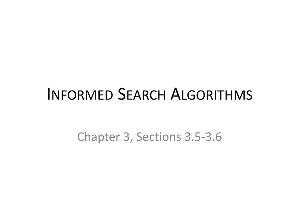
Class Exercise: Wooden Railway Set Track pieces from wooden railway set:
Q1: Suppose the pieces fit together exactly. Give formulation of the task as a search problem
x 12
x 16
x 12 x 2 x 2
(Curved pieces can be flipped)
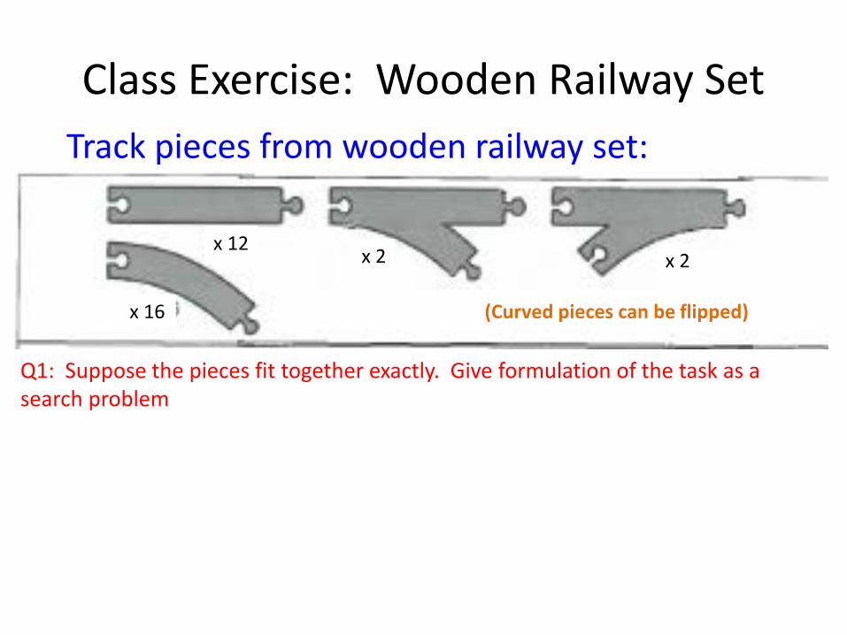
Class Exercise: Wooden Railway Set (con’t.)
Track pieces from wooden railway set:
Q2: Identify a suitable uninformed search algorithm for this task, and explain why it is suitable.
x 12
x 16
x 12 x 2 x 2
(Curved pieces can be flipped)
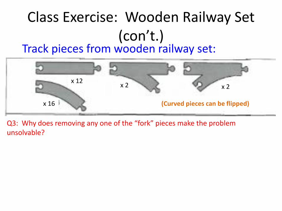
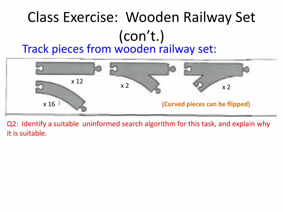
Class Exercise: Wooden Railway Set (con’t.)
Track pieces from wooden railway set:
Q3: Why does removing any one of the “fork” pieces make the problem unsolvable?
x 12
x 16
x 12 x 2 x 2
(Curved pieces can be flipped)
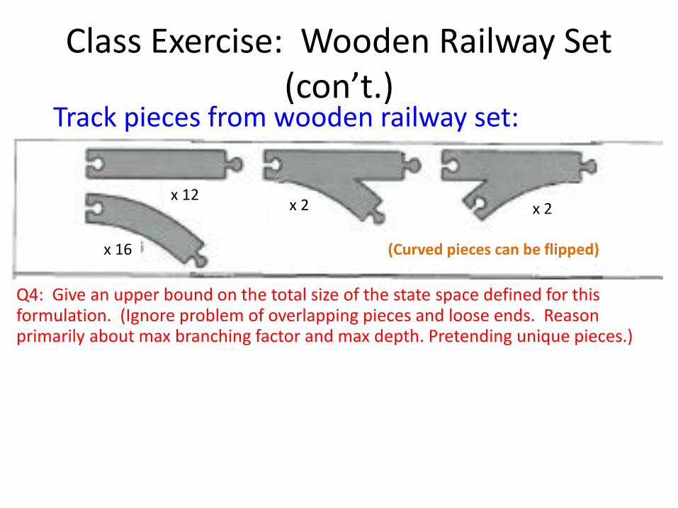
Class Exercise: Wooden Railway Set (con’t.)
Track pieces from wooden railway set:
Q4: Give an upper bound on the total size of the state space defined for this formulation. (Ignore problem of overlapping pieces and loose ends. Reason primarily about max branching factor and max depth. Pretending unique pieces.)
x 12
x 16
x 12 x 2 x 2
(Curved pieces can be flipped)
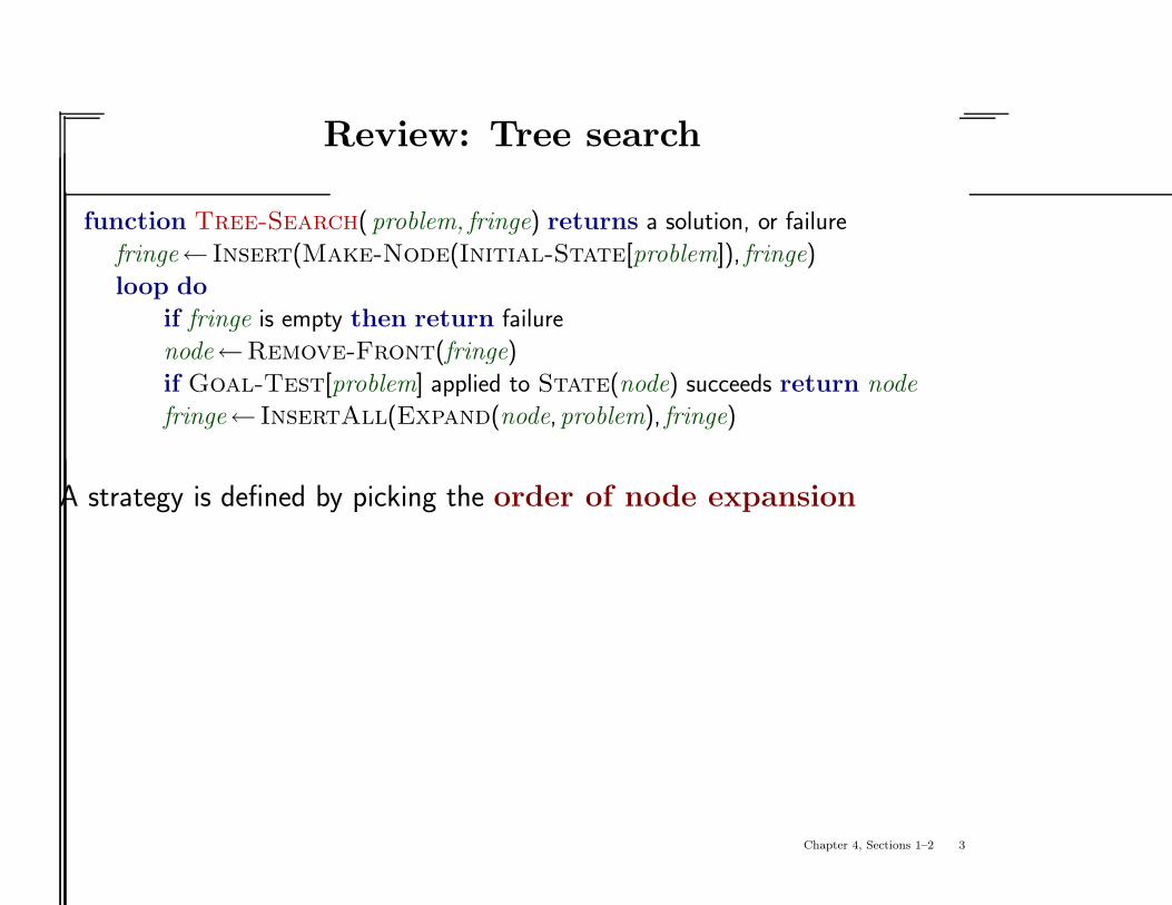
Review: Tree search
function Tree-Search( problem, fringe) returns a solution, or failure
fringe← Insert(Make-Node(Initial-State[problem]), fringe)
loop do
if fringe is empty then return failure
node←Remove-Front(fringe)
if Goal-Test[problem] applied to State(node) succeeds return node
fringe← InsertAll(Expand(node,problem), fringe)
A strategy is defined by picking the order of node expansion
Chapter 4, Sections 1–2 3
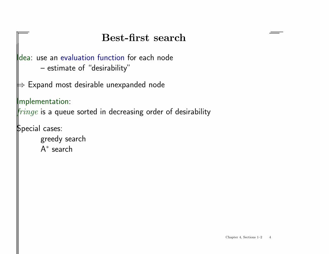
Best-first search
Idea: use an evaluation function for each node– estimate of “desirability”
⇒ Expand most desirable unexpanded node
Implementation:fringe is a queue sorted in decreasing order of desirability
Special cases:greedy searchA∗ search
Chapter 4, Sections 1–2 4
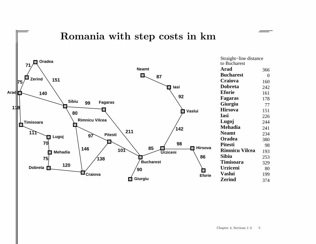
Romania with step costs in km
Bucharest
Giurgiu
Urziceni
Hirsova
Eforie
NeamtOradea
Zerind
Arad
Timisoara
LugojMehadia
DobretaCraiova
Sibiu
Fagaras
PitestiRimnicu Vilcea
Vaslui
Iasi
Straight−line distanceto Bucharest
0160242161
77151
241
366
193
178
25332980
199
244
380
226
234
374
98
Giurgiu
UrziceniHirsova
Eforie
Neamt
Oradea
Zerind
Arad
Timisoara
Lugoj
Mehadia
Dobreta
Craiova
Sibiu Fagaras
Pitesti
Vaslui
Iasi
Rimnicu Vilcea
Bucharest
71
75
118
111
70
75120
151
140
99
80
97
101
211
138
146 85
90
98
142
92
87
86
Chapter 4, Sections 1–2 5
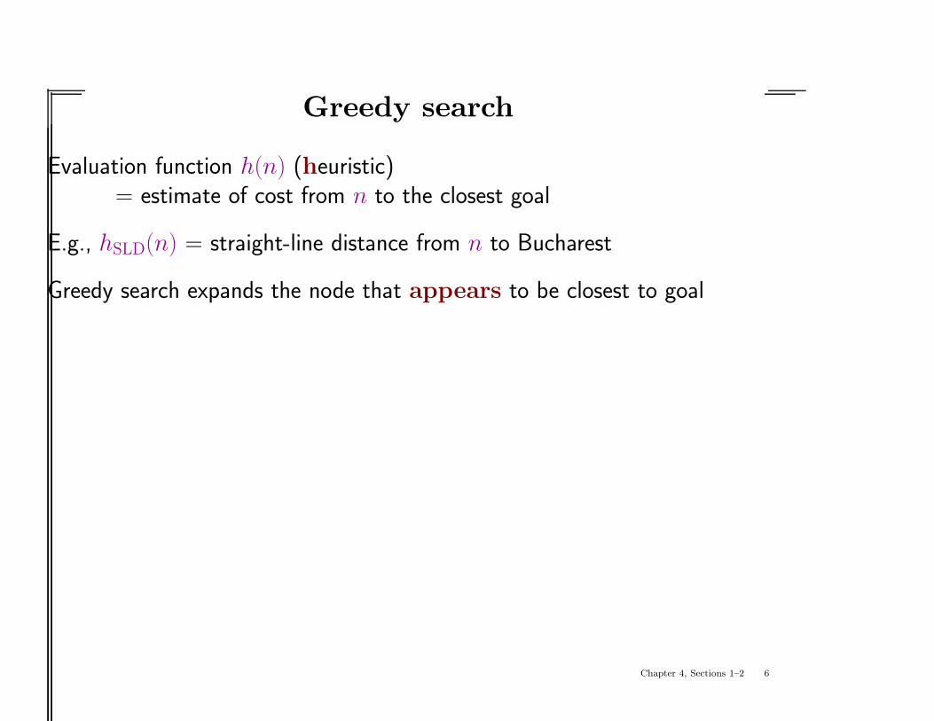
Greedy search
Evaluation function h(n) (heuristic)= estimate of cost from n to the closest goal
E.g., hSLD(n) = straight-line distance from n to Bucharest
Greedy search expands the node that appears to be closest to goal
Chapter 4, Sections 1–2 6
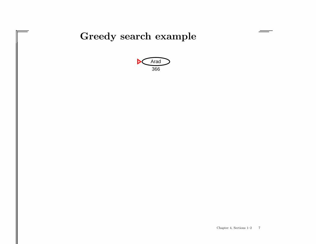
Greedy search example
Arad
366
Chapter 4, Sections 1–2 7
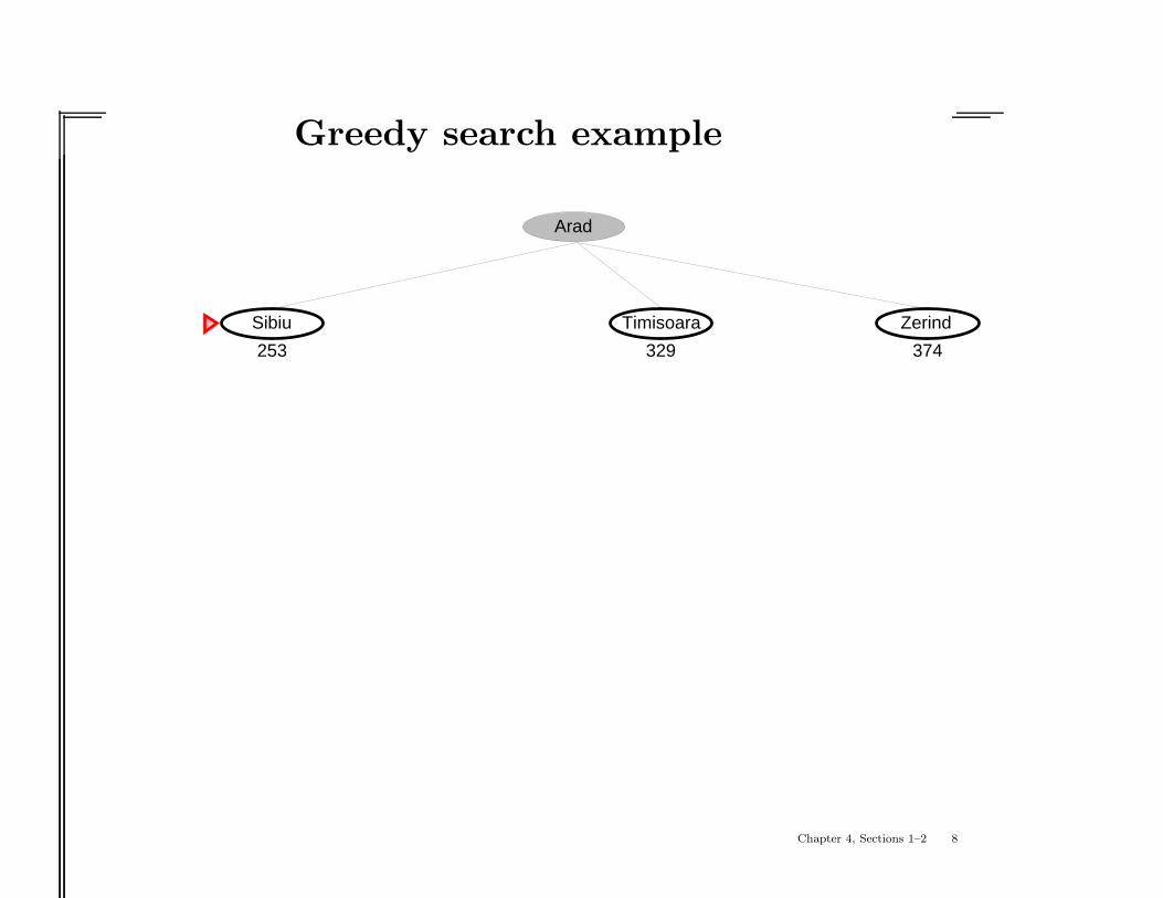
Greedy search example
Zerind
Arad
Sibiu Timisoara
253 329 374
Chapter 4, Sections 1–2 8
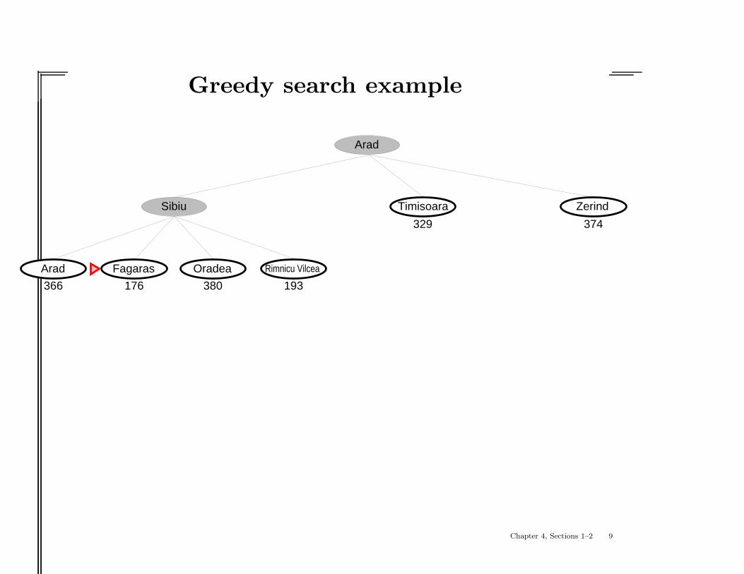
Greedy search example
Rimnicu Vilcea
Zerind
Arad
Sibiu
Arad Fagaras Oradea
Timisoara
329 374
366 176 380 193
Chapter 4, Sections 1–2 9
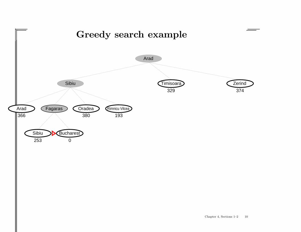
Greedy search example
Rimnicu Vilcea
Zerind
Arad
Sibiu
Arad Fagaras Oradea
Timisoara
Sibiu Bucharest
329 374
366 380 193
253 0
Chapter 4, Sections 1–2 10
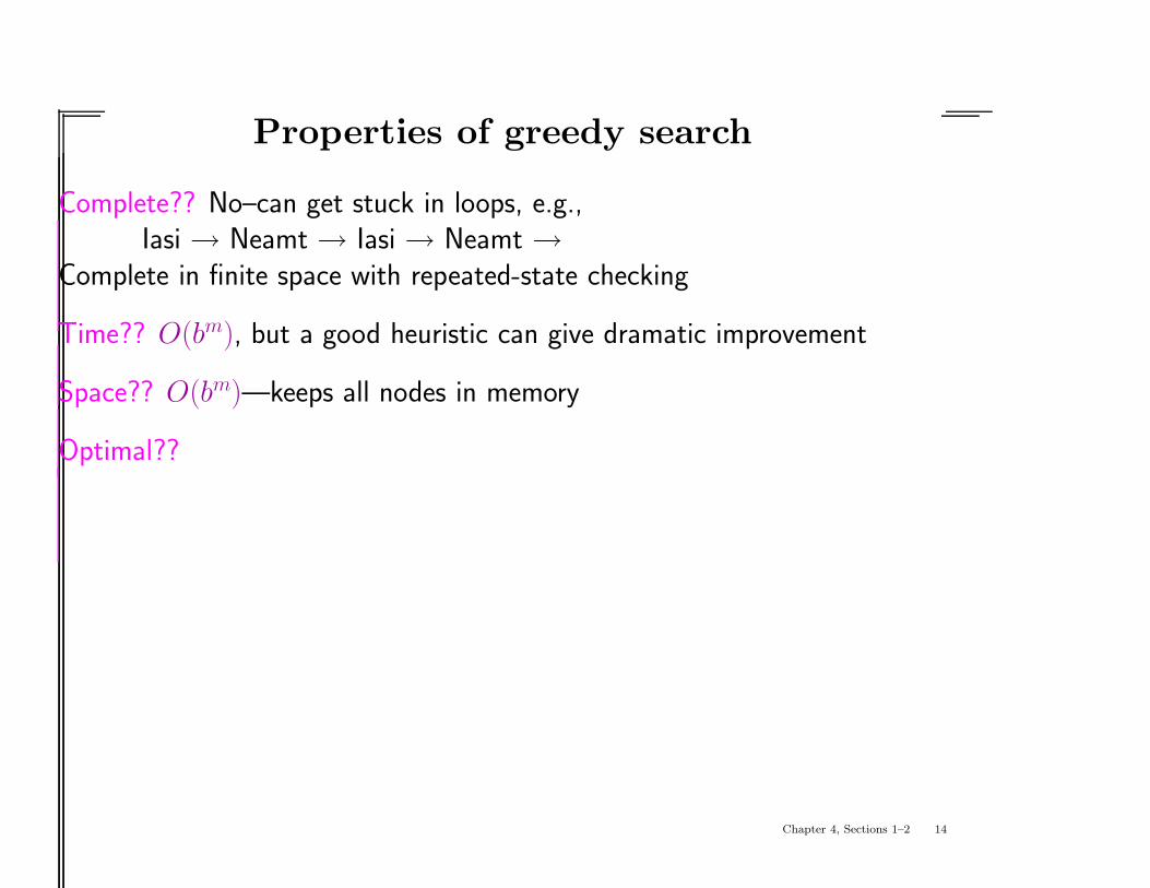
Properties of greedy search
Complete??
Chapter 4, Sections 1–2 11
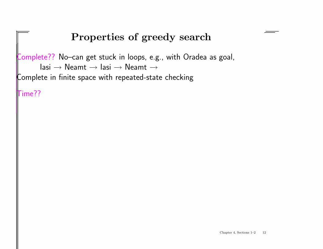
Properties of greedy search
Complete?? No–can get stuck in loops, e.g., with Oradea as goal,Iasi → Neamt → Iasi → Neamt →
Complete in finite space with repeated-state checking
Time??
Chapter 4, Sections 1–2 12
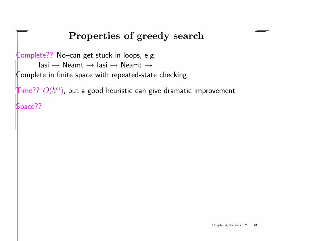
Properties of greedy search
Complete?? No–can get stuck in loops, e.g.,Iasi → Neamt → Iasi → Neamt →
Complete in finite space with repeated-state checking
Time?? O(bm), but a good heuristic can give dramatic improvement
Space??
Chapter 4, Sections 1–2 13
Properties of greedy search
Complete?? No–can get stuck in loops, e.g.,Iasi → Neamt → Iasi → Neamt →
Complete in finite space with repeated-state checking
Time?? O(bm), but a good heuristic can give dramatic improvement
Space?? O(bm)—keeps all nodes in memory
Optimal??
Chapter 4, Sections 1–2 14
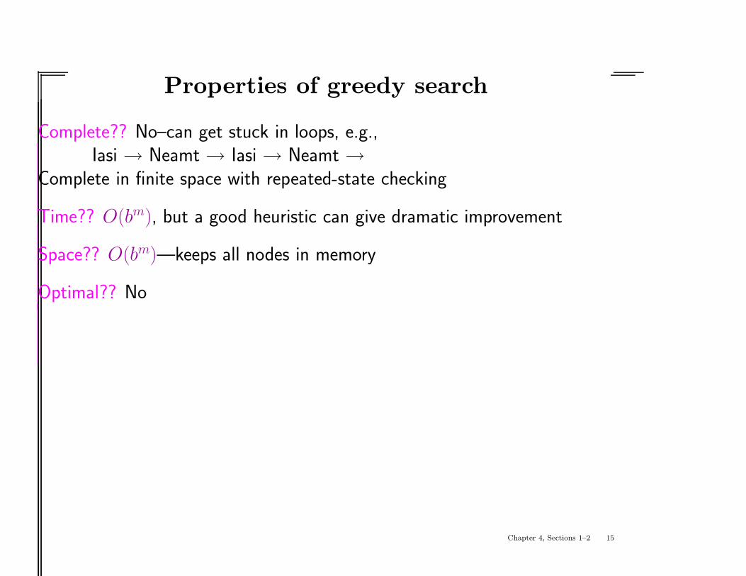
Properties of greedy search
Complete?? No–can get stuck in loops, e.g.,Iasi → Neamt → Iasi → Neamt →
Complete in finite space with repeated-state checking
Time?? O(bm), but a good heuristic can give dramatic improvement
Space?? O(bm)—keeps all nodes in memory
Optimal?? No
Chapter 4, Sections 1–2 15
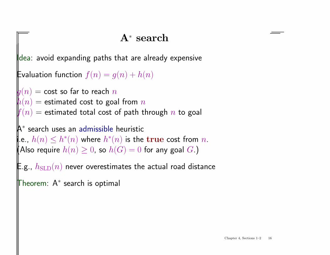
A∗ search
Idea: avoid expanding paths that are already expensive
Evaluation function f(n) = g(n) + h(n)
g(n) = cost so far to reach n
h(n) = estimated cost to goal from n
f(n) = estimated total cost of path through n to goal
A∗ search uses an admissible heuristici.e., h(n) ≤ h∗(n) where h∗(n) is the true cost from n.(Also require h(n) ≥ 0, so h(G) = 0 for any goal G.)
E.g., hSLD(n) never overestimates the actual road distance
Theorem: A∗ search is optimal
Chapter 4, Sections 1–2 16

A∗ search example
Arad
366=0+366
Chapter 4, Sections 1–2 17

A∗ search example
Zerind
Arad
Sibiu Timisoara
447=118+329 449=75+374393=140+253
Chapter 4, Sections 1–2 18
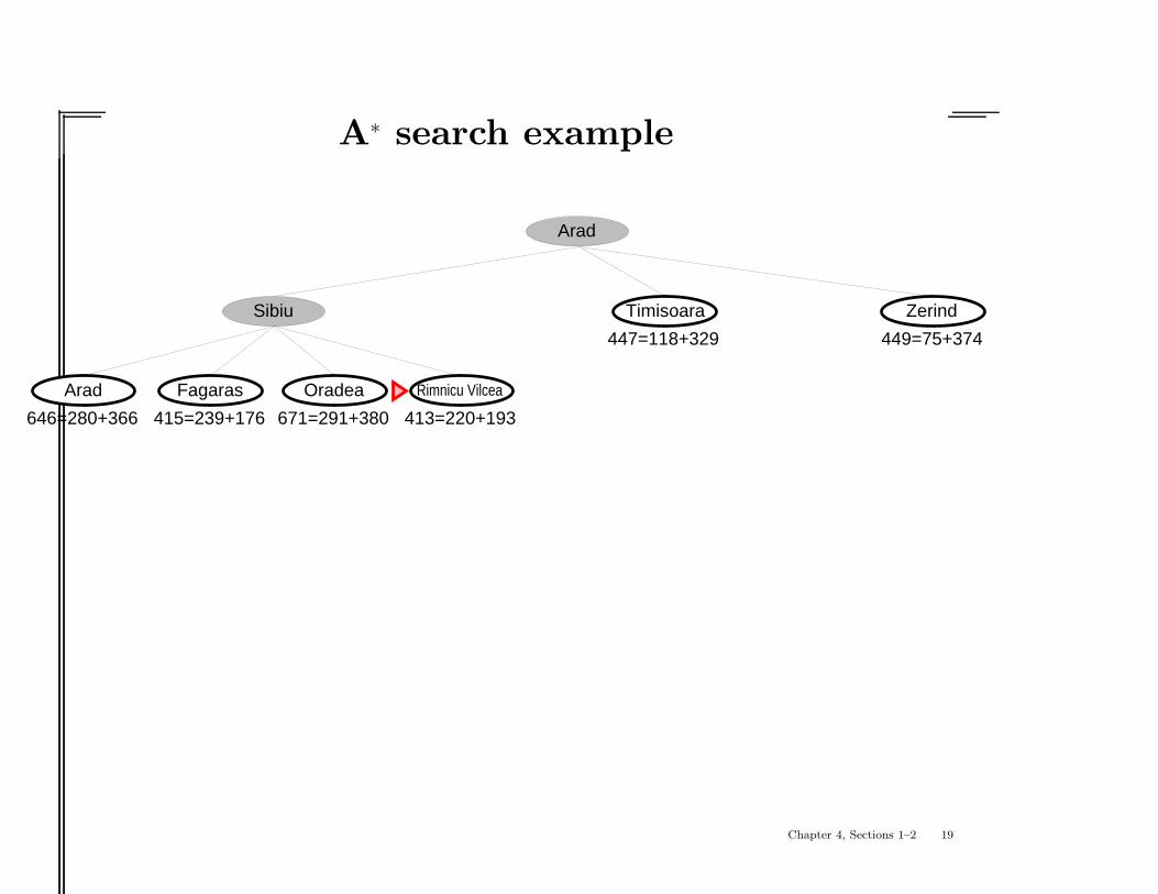
A∗ search example
Zerind
Arad
Sibiu
Arad
Timisoara
Rimnicu VilceaFagaras Oradea
447=118+329 449=75+374
646=280+366 413=220+193415=239+176 671=291+380
Chapter 4, Sections 1–2 19
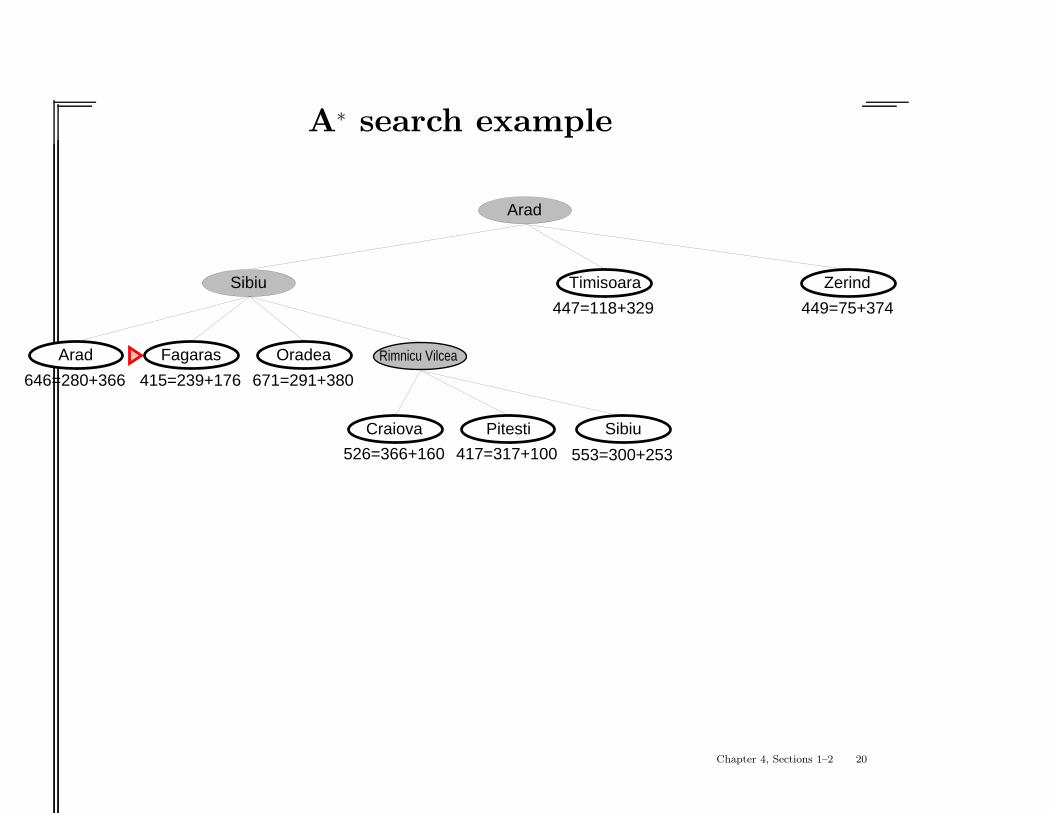
A∗ search example
Zerind
Arad
Sibiu
Arad
Timisoara
Fagaras Oradea
447=118+329 449=75+374
646=280+366 415=239+176
Rimnicu Vilcea
Craiova Pitesti Sibiu
526=366+160 553=300+253417=317+100
671=291+380
Chapter 4, Sections 1–2 20

A∗ search example
Zerind
Arad
Sibiu
Arad
Timisoara
Sibiu Bucharest
Rimnicu VilceaFagaras Oradea
Craiova Pitesti Sibiu
447=118+329 449=75+374
646=280+366
591=338+253 450=450+0 526=366+160 553=300+253417=317+100
671=291+380
Chapter 4, Sections 1–2 21
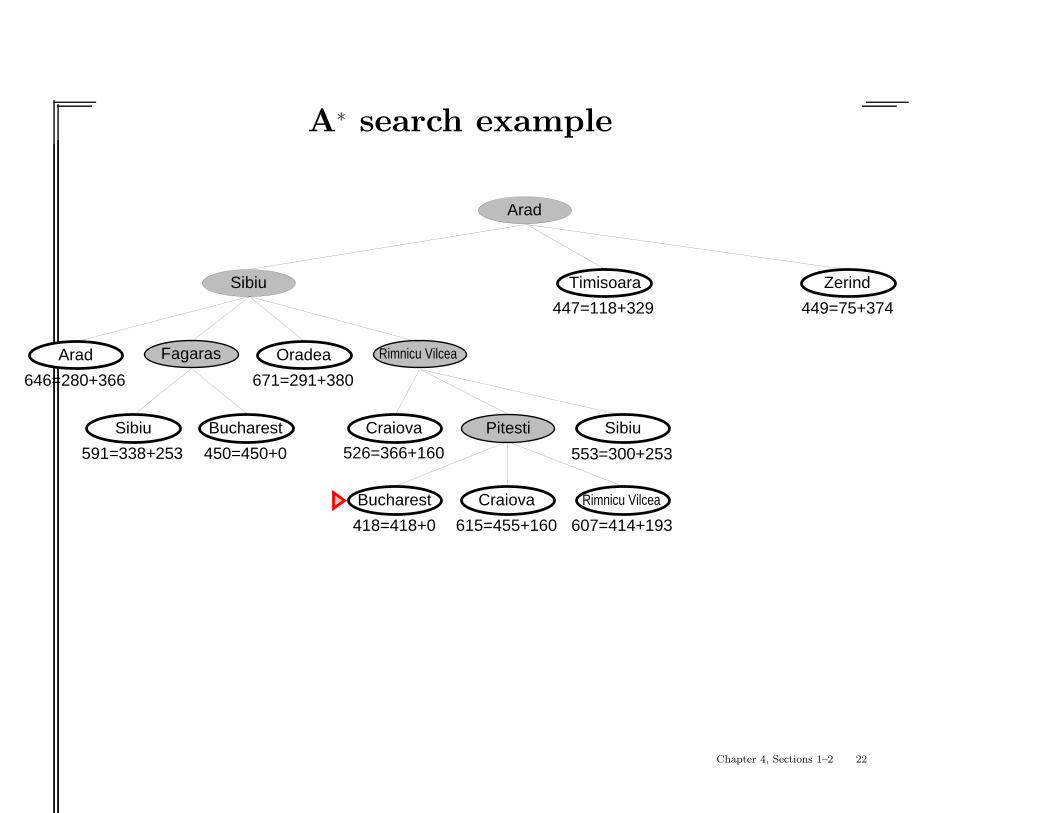
A∗ search example
Zerind
Arad
Sibiu
Arad
Timisoara
Sibiu Bucharest
Rimnicu VilceaFagaras Oradea
Craiova Pitesti Sibiu
Bucharest Craiova Rimnicu Vilcea
418=418+0
447=118+329 449=75+374
646=280+366
591=338+253 450=450+0 526=366+160 553=300+253
615=455+160 607=414+193
671=291+380
Chapter 4, Sections 1–2 22
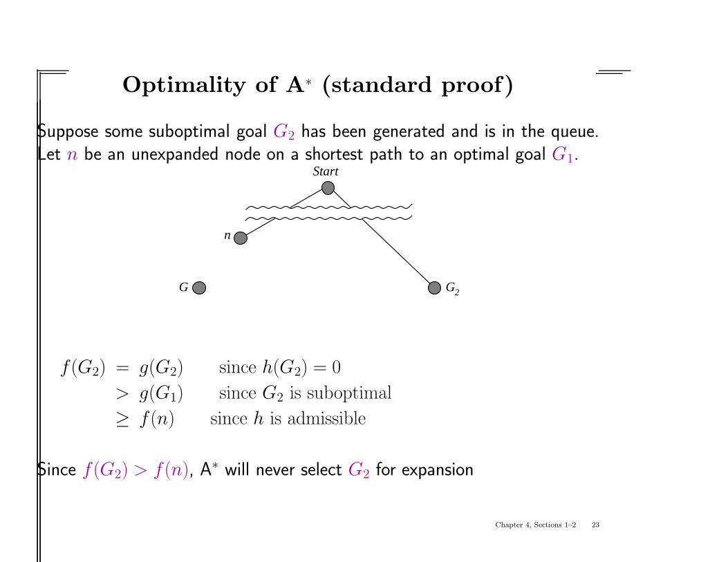
Optimality of A∗ (standard proof)
Suppose some suboptimal goal G2 has been generated and is in the queue.Let n be an unexpanded node on a shortest path to an optimal goal G1.
G
n
G2
Start
f(G2) = g(G2) since h(G2) = 0
> g(G1) since G2 is suboptimal
≥ f(n) since h is admissible
Since f(G2) > f(n), A∗ will never select G2 for expansion
Chapter 4, Sections 1–2 23
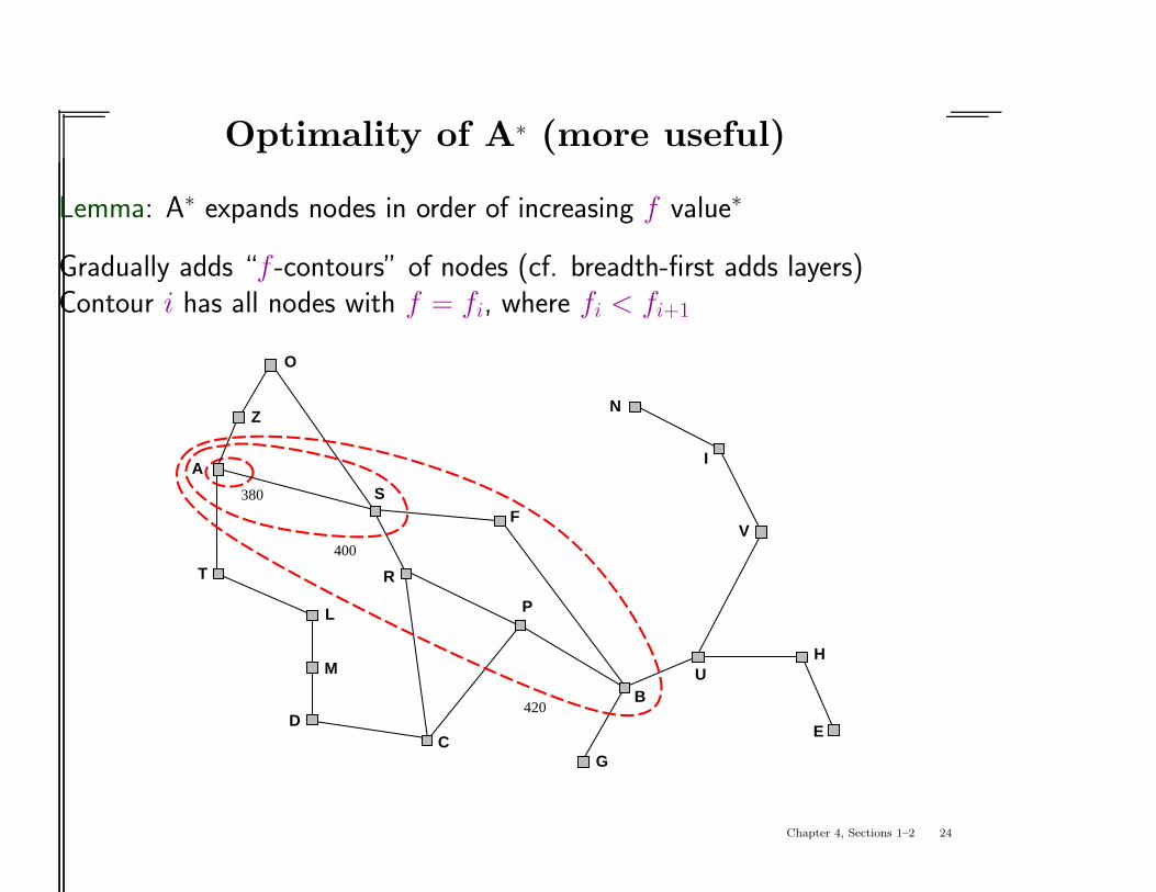
Optimality of A∗ (more useful)
Lemma: A∗ expands nodes in order of increasing f value∗
Gradually adds “f -contours” of nodes (cf. breadth-first adds layers)Contour i has all nodes with f = fi, where fi < fi+1
O
Z
A
T
L
M
DC
R
F
P
G
BU
H
E
V
I
N
380
400
420
S
Chapter 4, Sections 1–2 24
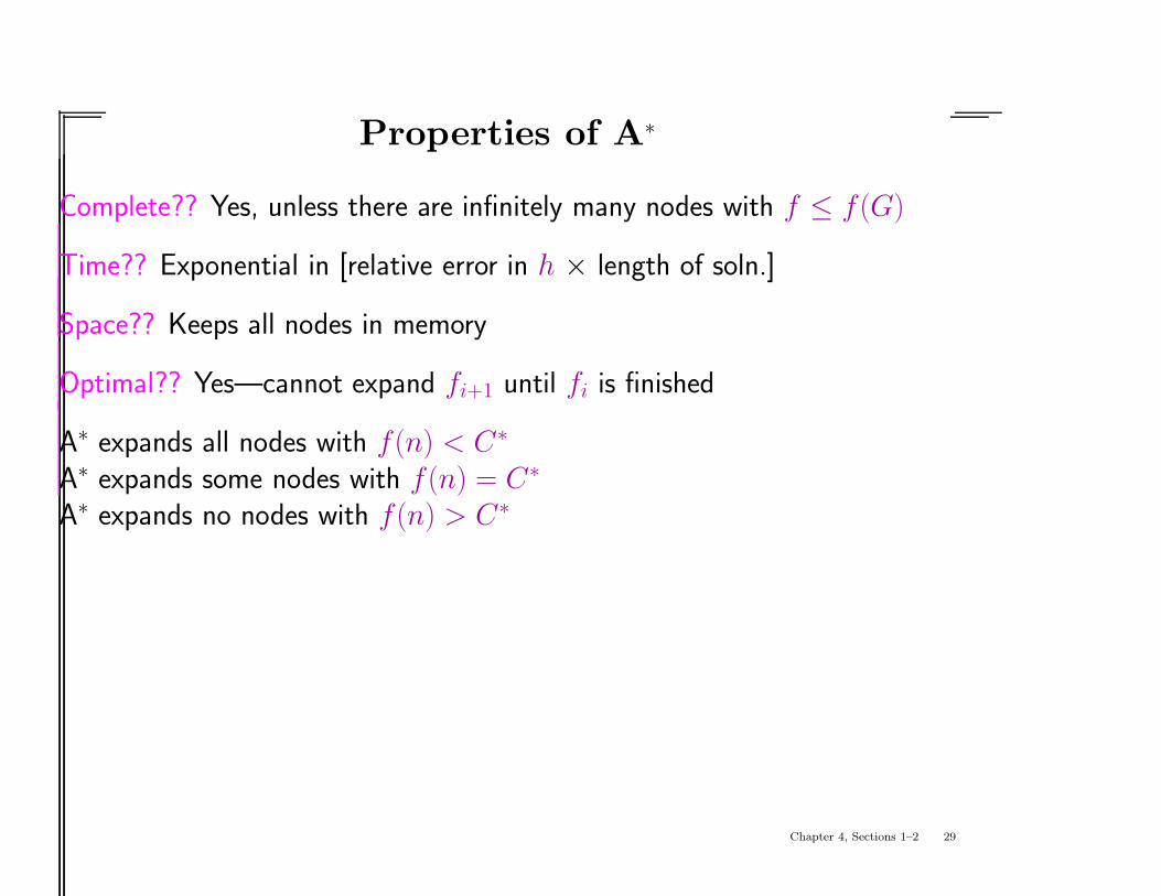
Properties of A∗
Complete??
Chapter 4, Sections 1–2 25
Properties of A∗
Complete?? Yes, unless there are infinitely many nodes with f ≤ f(G)
Time??
Chapter 4, Sections 1–2 26
Properties of A∗
Complete?? Yes, unless there are infinitely many nodes with f ≤ f(G)
Time?? Exponential in [relative error in h × length of soln.]
Space??
Chapter 4, Sections 1–2 27
Properties of A∗
Complete?? Yes, unless there are infinitely many nodes with f ≤ f(G)
Time?? Exponential in [relative error in h × length of soln.]
Space?? Keeps all nodes in memory
Optimal??
Chapter 4, Sections 1–2 28
Properties of A∗
Complete?? Yes, unless there are infinitely many nodes with f ≤ f(G)
Time?? Exponential in [relative error in h × length of soln.]
Space?? Keeps all nodes in memory
Optimal?? Yes—cannot expand fi+1 until fi is finished
A∗ expands all nodes with f(n) < C∗
A∗ expands some nodes with f(n) = C∗
A∗ expands no nodes with f(n) > C∗
Chapter 4, Sections 1–2 29
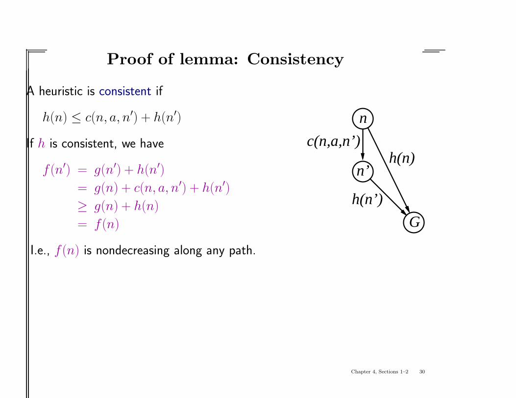
Proof of lemma: Consistency
A heuristic is consistent if
n
c(n,a,n’)
h(n’)
h(n)
G
n’
h(n) ≤ c(n, a, n′) + h(n′)
If h is consistent, we have
f(n′) = g(n′) + h(n′)
= g(n) + c(n, a, n′) + h(n′)
≥ g(n) + h(n)
= f(n)
I.e., f(n) is nondecreasing along any path.
Chapter 4, Sections 1–2 30
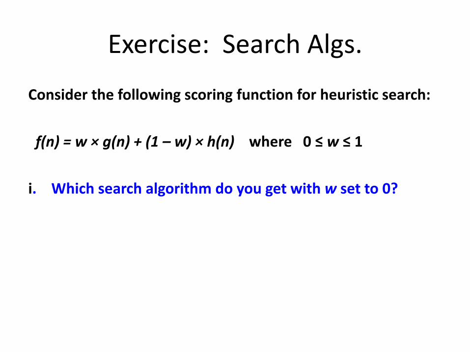
Exercise: Search Algs.
Consider the following scoring function for heuristic search: f(n) = w × g(n) + (1 – w) × h(n) where 0 ≤ w ≤ 1 i. Which search algorithm do you get with w set to 0?

Exercise: Various Search Algs.
1) Prove that breadth-first search is a special case of uniform-cost search.
Exercise: Various Search Algs.
2) Prove that breadth-first search, depth-first search, and uniform-cost search are special cases of best-first search.
Exercise: Various Search Algs.
3) Prove that uniform-cost search is a special case of A* search
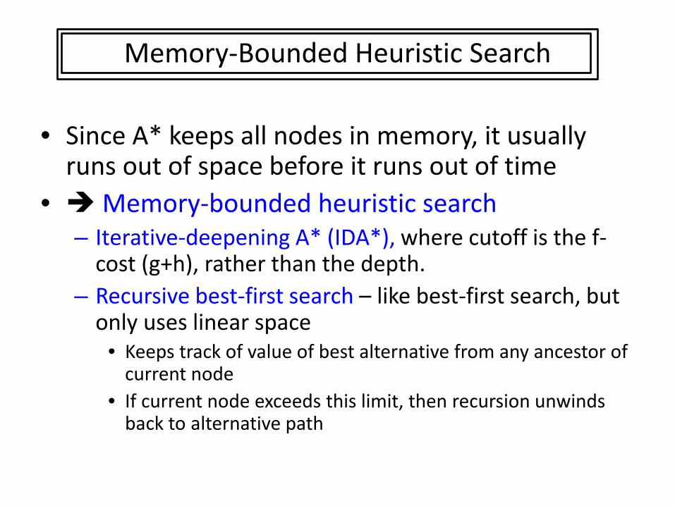
• Since A* keeps all nodes in memory, it usually runs out of space before it runs out of time
• Memory-bounded heuristic search – Iterative-deepening A* (IDA*), where cutoff is the f-
cost (g+h), rather than the depth. – Recursive best-first search – like best-first search, but
only uses linear space • Keeps track of value of best alternative from any ancestor of
current node • If current node exceeds this limit, then recursion unwinds
back to alternative path
Memory-Bounded Heuristic Search
• Problem: IDA* and RBFS don’t use all the memory they could, leading to re-evaluation of states multiple times
• Memory-Bounded A* (MA*), and Simplified MA* (SMA*) are better.
Memory-Bounded Heuristic Search
• Proceeds like A*, expanding best leaf until memory is full
• Then, it drops worst leaf node (i.e., one with highest f value)
• If all leaf nodes have same f value, then delete the oldest node
• SMA* – Is complete if d is less than memory size – Is optimal if any optimal solution is reachable
• Otherwise, returns best reachable solution • But, on hard problems, SMA* thrashes between many
candidate solution paths – Tradeoff between computation and memory
Simplified MA* (SMA*)
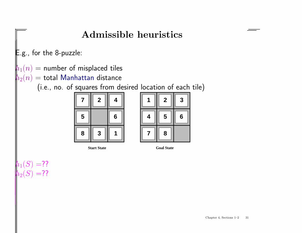
Admissible heuristics
E.g., for the 8-puzzle:
h1(n) = number of misplaced tilesh2(n) = total Manhattan distance
(i.e., no. of squares from desired location of each tile)
2
Start State Goal State
51 3
4 6
7 8
5
1
2
3
4
6
7
8
5
h1(S) =??h2(S) =??
Chapter 4, Sections 1–2 31

Admissible heuristics
E.g., for the 8-puzzle:
h1(n) = number of misplaced tilesh2(n) = total Manhattan distance
(i.e., no. of squares from desired location of each tile)
2
Start State Goal State
51 3
4 6
7 8
5
1
2
3
4
6
7
8
5
h1(S) =?? 6h2(S) =?? 4+0+3+3+1+0+2+1 = 14
Chapter 4, Sections 1–2 32
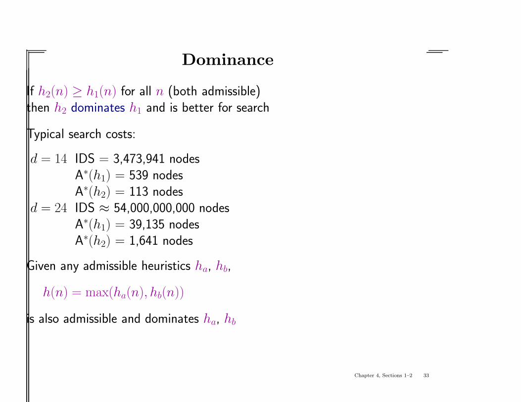
Dominance
If h2(n) ≥ h1(n) for all n (both admissible)then h2 dominates h1 and is better for search
Typical search costs:
d = 14 IDS = 3,473,941 nodesA∗(h1) = 539 nodesA∗(h2) = 113 nodes
d = 24 IDS ≈ 54,000,000,000 nodesA∗(h1) = 39,135 nodesA∗(h2) = 1,641 nodes
Given any admissible heuristics ha, hb,
h(n) = max(ha(n), hb(n))
is also admissible and dominates ha, hb
Chapter 4, Sections 1–2 33
Relaxed problems
Admissible heuristics can be derived from the exact
solution cost of a relaxed version of the problem
If the rules of the 8-puzzle are relaxed so that a tile can move anywhere,then h1(n) gives the shortest solution
If the rules are relaxed so that a tile can move to any adjacent square,then h2(n) gives the shortest solution
Key point: the optimal solution cost of a relaxed problemis no greater than the optimal solution cost of the real problem
Chapter 4, Sections 1–2 34
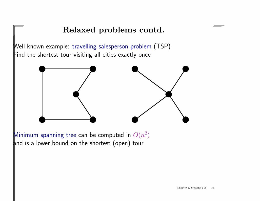
Relaxed problems contd.
Well-known example: travelling salesperson problem (TSP)Find the shortest tour visiting all cities exactly once
Minimum spanning tree can be computed in O(n2)and is a lower bound on the shortest (open) tour
Chapter 4, Sections 1–2 35
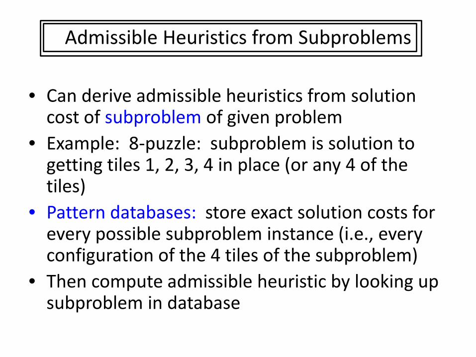
• Can derive admissible heuristics from solution cost of subproblem of given problem
• Example: 8-puzzle: subproblem is solution to getting tiles 1, 2, 3, 4 in place (or any 4 of the tiles)
• Pattern databases: store exact solution costs for every possible subproblem instance (i.e., every configuration of the 4 tiles of the subproblem)
• Then compute admissible heuristic by looking up subproblem in database
Admissible Heuristics from Subproblems
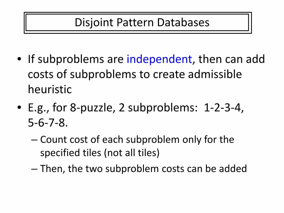
• If subproblems are independent, then can add costs of subproblems to create admissible heuristic
• E.g., for 8-puzzle, 2 subproblems: 1-2-3-4, 5-6-7-8. – Count cost of each subproblem only for the
specified tiles (not all tiles) – Then, the two subproblem costs can be added
Disjoint Pattern Databases
Summary
Heuristic functions estimate costs of shortest paths
Good heuristics can dramatically reduce search cost
Greedy best-first search expands lowest h
– incomplete and not always optimal
A∗ search expands lowest g + h
– complete and optimal– also optimally efficient (up to tie-breaks, for forward search)
Admissible heuristics can be derived from exact solution of relaxed problems
Chapter 4, Sections 1–2 36

Reading Assignment
• For Thursday: Chapter 4.3-4.5 (we’re skipping 4.1-4.2)
• For next week: Chapter 5